Linear and Nonlinear Event-Triggered Extended State Observers for Uncertain Stochastic Systems

Abstract

In this paper, linear and nonlinear event-triggered extended state observers are designed for a class of uncertain stochastic systems driven by bounded and colored noises. Two event-generators with an ensured positive minimum inter-event time for every sample path solution of the stochastic systems, are proposed for the designs of linear and nonlinear event-triggered extended state observers, respectively. The mean square and almost sure convergence of the estimation errors of unmeasured state and stochastic total disturbance including internal uncertainty and external stochastic noises is presented with rigorous theoretical proofs. Compared with the linear event-triggered extended state observer, the theoretical results show that the nonlinear one via homogeneity possesses higher estimation accuracy but is at the price of higher triggering frequency. Some numerical simulations are performed to authenticate the theoretical results.

I Introduction

Owing to the ubiquity of uncertainties and disturbances in practical engineering systems, disturbance rejection for uncertain systems has been one of mainstream topics in recent decades in the control community. Active disturbance rejection control (ADRC) [1], a highly novel control technology based on estimation/compensation strategy, can cope with uncertainties and disturbances in large scale. The significance of ADRC has been validated by considerable number of engineering applications. The key component part of ADRC is the extended state observer (ESO) designed to be linear or nonlinear, aiming at real-time estimation of not only unmeasured state but also total disturbance (extended state) affecting system performance; Based on the estimates obtained via ESO, an active anti-disturbance control constructed by a feedback control and a compensator can be designed for disturbance rejection and prospective control objective. Therefore, the theoretical foundation for the convergence of ESO is extremely important in ADRC’s theory and applications.

The convergence of linear and common nonlinear ESOs for uncertain systems has been investigated in the past two decades, see [2, 3] and the references therein. The convergence of linear ESO and nonlinear ESOs based on an exponentially stable system and finite-time stable one for uncertain stochastic systems have also been researched in [4, 5]. It should be noted that most of these works concerning the design and theoretical analysis of ESO are based on continuous-time output measurement. However, in prevailing networked control systems or digital control systems, one of the crucial problems is to reduce the utilization of communication/computation resources. This greatly spurs the current research of event-triggering mechanism (ETM) in the estimation and control of systems, primarily on account of its advantage in saving communication/computation resources (see, e.g., [6, 7, 8, 9] and references therein).

The convergence of a nonlinear event-triggered ESO for a class of uncertain systems has been developed in [6], where the nonlinear gain functions are constructed by an exponentially stable system and cover the linear ones as a special case. Nevertheless, it is admittedly more realistic that uncertainties and disturbances are often stochastic in practice. One of the momentous problems for the ETM to be practical and feasible is to avoid the Zeno phenomenon (i.e., the triggering conditions are satisfied infinite times in finite time), which would bring challenging obstacle in developing the event-triggered ESO for uncertain stochastic systems. This is because when there exist stochastic noises, each sample path of system state may change variously even for the deterministic initial condition; Specifically, the execution/sampling times and the inter-execution times depending on sample path, are stochastic but not deterministic, so that obtaining a positive lower bound for the stochastic inter-execution times (i.e., excluding Zeno phenomenon) is very sophisticated or even impossible. Recently, novel ETM with dwell time (time-regularization) and periodic ETM have been proposed for stochastic systems, which force the ETM to allow a positive minimum inter-event time, see, e.g., [7, 8, 9]. The Zeno phenomenon can be directly excluded in these design frameworks, while the theoretical analysis becomes much more difficult.

On the other hand, compared with the nonlinear ESO in [6] that is an almost linear one, a more widely used nonlinear ESO based on a finite-time stable system via homogeneity has been shown to be with higher estimation accuracy and better noise-tolerant performance [3, 5, 19]; The convergence of the nonlinear event-triggered ESO via homogeneity for uncertain systems is still unsolved, where the stochastic counterpart is more general and complex.

Motivated by aforementioned research status, in this paper we develop both the linear and nonlinear event-triggered ESOs for a class of uncertain stochastic systems driven by bounded and colored noises. The main contributions and novelties can be summed up as follows: a) The uncertain stochastic systems are subject to large-scale stochastic total disturbance which is the total nonlinear coupling effects of unmodeled dynamics, external deterministic disturbance, bounded noise and colored noise; b) Novel linear/nonlinear event-triggered ESOs are designed for the uncertain stochastic systems, and the mean square and almost sure convergence in the transient process is presented with rigorous theoretical proofs; c) The theoretical results reveal that the nonlinear event-triggered ESO via homogeneity is with higher estimation accuracy but higher triggering frequency compared with the linear one.

This paper will be proceed as below. The problem formulation and some preliminaries are presented in Section II. The designs of linear and nonlinear event-triggered ESOs and convergence results are given in Section III. Some numerical simulations are performed to validate the rationality of the theoretical results in Section IV, with the concluding remarks be followed up in Section V. For the sake of readability, theoretical proofs are arranged in Appendix A and Appendix B.

II Problem formulation and preliminaries

The following notations are used throughout the paper. $\mathbb{E}$ denotes the mathematical expectation; $|Z|$ represents the absolute value of a scalar $Z$, and $\|Z\|$ represents the Euclidean norm of a vector $Z$; $I_{n}$ denotes the $n$-dimensional identity matrix; $\lambda_{\min}(Z)$ and $\lambda_{\max}(Z)$ represent the minimum eigenvalue and maximum eigenvalue of a positive definite matrix $Z$; $a\wedge b:=\min\{a,b\}$; $\langle\vartheta\rangle^{s}:={\rm sign}(\vartheta)|\vartheta|^{s}$ for all $\vartheta\in\mathbb{R}$ and any $s>0$; $\mathbb{I}_{\Omega_{0}}$ denotes an indicator function with the function value being $1$ in the domain $\Omega_{0}$ and being $0$ otherwise; $0_{s}$ represent the $1\times s$ row vector with all components to be zero.

To deal with the convergence of the nonlinear ESO constructed via homogeneity, the definitions of homogeneity and some preliminary lemmas are introduced as follows.

Definition II.1.

([10]) The zero equilibrium of the following system

$$\dot{\vartheta}(t)=\psi(\vartheta(t)),\ \vartheta(0)=\vartheta_{0}\in\mathbb{R}^{s}$$ (1)

with $\psi\in C(\mathbb{R}^{s};\mathbb{R}^{s})$ and $\psi(0_{s})=0_{s}$, is said to be globally finite-time stable, if the zero equilibrium of system (1) is Lyapunov stable and for any $\vartheta_{0}\in\mathbb{R}^{s}$, there exists $T(\vartheta_{0})>0$ such that the solution of (1) satisfies that $\lim_{t\rightarrow T(\vartheta_{0})}\vartheta(t)=0_{s}$ and $\vartheta(t)=0_{s}$ for all $t\in[T(\vartheta_{0}),\infty)$.

Definition II.2.

([11]) A function $W:\mathbb{R}^{s}\to\mathbb{R}$ is said to be homogeneous of degree $\theta$ with respect to weights $\{w_{l}>0\}_{l=1}^{s}$, if $W(\lambda^{w_{1}}\vartheta_{1},\lambda^{w_{2}}\vartheta_{2},\cdots,\lambda^{w_{s}}\vartheta_{s})=\lambda^{\theta}W(\vartheta_{1},\vartheta_{2},\cdots,\vartheta_{s})$ for all $\lambda>0$ and all $(\vartheta_{1},\cdots,\vartheta_{s})\in\mathbb{R}^{s}$. A vector field $W:\mathbb{R}^{s}\to\mathbb{R}^{s}$ is said to be homogeneous of degree $\theta$ with respect to weights $\{w_{l}>0\}_{l=1}^{s}$, if for all $l=1,\cdots,s$, the $l$-th component $W_{l}$ is a homogeneous function of degree $\theta+w_{l}$, that is, $W_{l}(\lambda^{w_{1}}\vartheta_{1},\lambda^{w_{2}}\vartheta_{2},\cdots,\lambda^{w_{s}}\vartheta_{s})=\lambda^{\theta+w_{l}}W_{l}(\vartheta_{1},\vartheta_{2},\cdots,\vartheta_{s})$ for all $\lambda>0$ and all $(\vartheta_{1},\cdots,\vartheta_{s})\in\mathbb{R}^{s}$. The system (1) is homogeneous of degree $\theta$ if the vector field $\psi$ is homogeneous of degree $\theta$.

Lemma II.1.

([11, Theorem 2] or [12, Theorem 6.2]) If system (1) is homogeneous of degree $\theta$ with weights $\{w_{l}\}_{l=1}^{s}$, and its zero equilibrium is globally asymptotically stable, then for any $\mu>\max_{1\leq l\leq s}\{-\theta,w_{l}\}$, there exists a positive definite, radially unbounded function $W\in C^{1}(\mathbb{R}^{s};\mathbb{R})\cap C^{\infty}(\mathbb{R}^{s}\setminus\{0_{s}\};\mathbb{R})\$ such that $W$ is homogeneous of degree $\mu$ with respect to weights $\{w_{l}\}_{l=1}^{s}$, and the Lie derivative of $W(\vartheta)$ along the vector field $\psi$: $L_{\psi}W(\vartheta):=\nabla W(\vartheta)\psi(\vartheta)$ is negative definite.

Lemma II.2.

[12, Lemma 4.2] Let $W_{1},W_{2}:\mathbb{R}^{s}\to\mathbb{R}$ be continuous functions, homogeneous of degree $\theta_{1}>0,\theta_{2}>0$ with respect to the same weights respectively, and $W_{1}$ is positive definite. Then for each $\vartheta\in\mathbb{R}^{s}$, it holds that $(\min_{\{z\in\mathbb{R}^{s}:\;W_{1}(z)=1\}}W_{2}(z))(W_{1}(\vartheta))^{\frac{\theta_{2}}{\theta_{1}}}\leq W_{2}(\vartheta)\leq(\max_{\{z\in\mathbb{R}^{s}:\;W_{1}(z)=1\}}W_{2}(z))(W_{1}(\vartheta))^{\frac{\theta_{2}}{\theta_{1}}}$.

Lemma II.3.

[10, Lemma 8] If $\nu\in(1-\frac{1}{n},1)$, then the vector field

$$\Phi(\vartheta):=(\Phi_{1}(\vartheta),\cdots,\Phi_{n}(\vartheta),\Phi_{n+1}(\vartheta))$$ (2)

$$:=(\vartheta_{2}-a_{1}\left\langle\vartheta_{1}\right\rangle^{\nu},\cdots,\vartheta_{n+1}-a_{n}\left\langle\vartheta_{1}\right\rangle^{n\nu-(n-1)},$$ (3)

$$-a_{n+1}\left\langle\vartheta_{1}\right\rangle^{(n+1)\nu-n}),\forall\vartheta=(\vartheta_{1},\cdots,\vartheta_{n+1})\in\mathbb{R}^{n+1}$$ (4)

is homogeneous of degree $\nu-1$ with respect to weights $\{(l-1)\nu-(l-2)\}_{l=1}^{n+1}$.

Define

$$G=\begin{pmatrix}-a_{1}&1&0&\cdots&0\cr-a_{2}&0&1&\cdots&0\cr\cdots&\cdots&\cdots&\cdots&\cdots\cr-a_{n}&0&0&\ddots&1\cr-a_{n+1}&0&0&\cdots&0\end{pmatrix}_{(n+1)\times(n+1)}.$$ (5)

Lemma II.4.

[10, Theorem 10] For $\nu\in(1-\frac{1}{n},1)$, if the matrix $G$ in (5) is Hurwitz, then the system $\dot{\vartheta}(t)=\Phi(\vartheta(t))$ is globally finite-time stable.

Lemma II.5.

(The multi-dimensional Itô’s formula) [15, p.36, Theorem 6.4] Let $x(t)$ be a $n$-dimensional Itô process on $t\geq 0$ with the stochastic differential $dx(t)=f(t)dt+g(t)dB(t)$, where $f\in L^{1}([0,\infty);\mathbb{R}^{n})$, $g\in L^{2}([0,\infty);\mathbb{R}^{n\times m})$ and $B(t)$ is a $m$-dimensional standard Brownian motion. Let $V\in C^{2}(\mathbb{R}^{n};\mathbb{R})$. Then $V(x(t))$ is again an Itô process with the stochastic differential given by

$$dV(x(t))=[\frac{\partial V(x(t))}{\partial x}f(t)+\frac{1}{2}\mbox{Tr}\{g^{\top}(t)\frac{\partial^{2}V(x(t))}{\partial x^{2}}g(t)\}]dt$$ (6)

$$\hskip 28.45274pt+\frac{\partial V(x(t))}{\partial x}g(t)dB(t)\;$$ (7)

$$\hskip 19.91684pt=:\mathcal{L}V(x(t))dt+\frac{\partial V(x(t))}{\partial x}g(t)dB(t)\;\;\;a.s.$$ (8)

Remark II.1.

The definition of $\mathcal{L}V(x(t))$ in (6) will be used throughout the paper. It should be pointed out that we could not define the infinitesimal generator $\mathcal{L}V$ itself because some random coefficients brought by bounded and colored noises such as aforementioned $f(t)$ and $g(t)$ occurring in the stochastic differential. This would not cause any obstacle in the following theoretical analysis because we only use $\mathbb{E}\mathcal{L}V(x(t))=\frac{d\mathbb{E}V(x(t))}{dt}$ when $\int^{t}_{0}\frac{\partial V(x(s))}{\partial x}g(s)dB(s)$ is a martingale for each $t\geq 0$.

Let $(\Omega,\mathcal{F},\mathbb{F},P)$ be a complete filtered probability space with a filtration $\mathbb{F}=\{\mathcal{F}_{t}\}_{t\geq 0}$ on which two mutually independent one-dimensional standard Brownian motions $B_{i}(t)\;(i=1,2)$ are defined. In this paper, we consider a class of uncertain stochastic systems driven by bounded and colored noises as follows:

$$\left\{\begin{array}[]{l}\dot{x}_{1}(t)=x_{2}(t),\cr\dot{x}_{2}(t)=x_{3}(t),\cr\hskip 31.2982pt\vdots\cr\dot{x}_{n}(t)=f(t,x(t),v_{1}(t),v_{2}(t))+u(t),\cr y(t)=x_{1}(t),\end{array}\right.$$ (9)

where $x(t)=(x_{1}(t),\cdots,x_{n}(t))\in\mathbb{R}^{n}$, $u(t)\in\mathbb{R}$ and $y(t)\in\mathbb{R}$ are the state, control input and output measurement, respectively; $f:[0,\infty)\times\mathbb{R}^{n+2}\rightarrow\mathbb{R}$ is an unknown system function satisfying Assumption (A1); $v_{1}(t):=\sigma(t,B_{1}(t))$ defined by an unknown bounded function $\sigma:[0,\infty)\times\mathbb{R}\rightarrow\mathbb{R}$ satisfying Assumption (A2) is the bounded noise, and $v_{2}(t)$ is the colored noise that is the solution to an Itô-type stochastic differential equation (see, e.g., [13, p.426], [15, p.101]):

$$dv_{2}(t)=-\alpha_{1}v_{2}(t)dt+\alpha_{1}\sqrt{2\alpha_{2}}dB_{2}(t),$$ (10)

where $\alpha_{1}>0$ and $\alpha_{2}>0$ are constants representing the correlation time and the noise intensity, respectively. It is noteworthy that white noise as a stationary stochastic process that has zero mean and constant spectral density, is the generalized derivative of the Brownian motion (see, e.g., [16, p.51, Theorem 3.14]) and often used to represent stochastic disturbances in many scenes. However, the white noise could not invariably describe the stochastic disturbances emerging in practice due to the fact that its $\delta$-function correlation is an idealization of the correlations of real processes which often have finite, or even long, correlation time [13]. A more realistic stochastic noise could be an exponentially correlated process, which is known as aforementioned colored noise or Ornstein-Uhlenbeck process [13, 14].

Remark II.2.

This paper is the first effort on the event-triggered ESO for uncertain stochastic systems, where both the designs and analyses are substantially different from the deterministic counterpart in [6]. Therefore, similar to the plant considered in [6], this paper only considers the most foundational essential-integral-chain systems with matched uncertainties and disturbances which are widely considered in the theory and application research of ADRC, to focus on the new designs and theoretical analyses of linear and nonlinear event-triggered ESOs when uncertainties and disturbances are stochastic. As its development to more general systems like lower triangle nonlinear ones [3] and MIMO ones [5] which does not cause essential obstacle, is not the main concern of this paper.

III Linear and nonlinear event-triggered ESOs designs and main results

Define the stochastic total disturbance (extended state) of system (9): $x_{n+1}(t)=f(t,x(t),v_{1}(t),v_{2}(t))$, which contains total nonlinear coupling effects of unmodeled dynamics, external deterministic disturbance, bounded noise and colored noise. To estimate not only unmeasured state but also stochastic total disturbance of system (9), a linear event-triggered extended state observer (ESO) is designed as follows:

$$\left\{\begin{array}[]{l}\dot{\hat{x}}_{1}(t)=\hat{x}_{2}(t)+a_{1}r\left(y(t_{k})-\hat{x}_{1}(t)\right),\cr\dot{\hat{x}}_{2}(t)=\hat{x}_{3}(t)+a_{2}r^{2}\left(y(t_{k})-\hat{x}_{1}(t)\right),\cr\hskip 34.14322pt\vdots\cr\dot{\hat{x}}_{n}(t)=\hat{x}_{n+1}(t)+a_{n}r^{n}\left(y(t_{k})-\hat{x}_{1}(t)\right)+u(t),\cr\dot{\hat{x}}_{n+1}(t)=a_{n+1}r^{n+1}\left(y(t_{k})-\hat{x}_{1}(t)\right),\end{array}\right.$$ (11)

where $t\in[t_{k},t_{k+1}),\;k\in\mathbb{Z}^{+}$, $r$ is the tuning gain, and the parameters $a_{i}$’s are chosen such that the matrix $G$ defined in (5) is Hurwitz; $\hat{x}(t):=(\hat{x}_{1}(t),\cdots,\hat{x}_{n+1}(t))$ contains the estimates of the state $x(t)$ and the stochastic total disturbance $x_{n+1}(t)$; $t_{k}$’s are stochastic execution times (stopping times) determined by the following ETM

$$t_{k+1}=\inf\{t\geq t_{k}+\tau:\;|y(t)-y(t_{k})|\geq\theta r^{-(n+\frac{1}{2})}\},$$ (12)

with $t_{1}=0$, $\tau$ being a positive constant specified in the following Theorem III.1 and $\theta$ being any free positive tuning parameter. The nonlinear event-triggered ESO via homogeneity is designed as

$$\left\{\begin{array}[]{l}\dot{\hat{x}}_{1}(t)=\hat{x}_{2}(t)+\frac{a_{1}}{r^{n-1}}\left\langle r^{n}(y(t_{k})-\hat{x}_{1}(t))\right\rangle^{\nu},\cr\dot{\hat{x}}_{2}(t)=\hat{x}_{3}(t)+\frac{a_{2}}{r^{n-2}}\left\langle r^{n}(y(t_{k})-\hat{x}_{1}(t))\right\rangle^{2\nu-1},\cr\hskip 34.14322pt\vdots\cr\dot{\hat{x}}_{n}(t)=\hat{x}_{n+1}(t)+a_{n}\left\langle r^{n}(y(t_{k})-\hat{x}_{1}(t))\right\rangle^{n\nu-(n-1)}\cr\hskip 36.98866pt+u(t),\cr\dot{\hat{x}}_{n+1}(t)=a_{n+1}r\left\langle r^{n}(y(t_{k})-\hat{x}_{1}(t))\right\rangle^{(n+1)\nu-n},\end{array}\right.$$ (19)

where $t\in[t_{k},t_{k+1}),\;k\in\mathbb{Z}^{+}$, $r$ is the tuning gain, the parameters $a_{i}$’s are chosen such that the matrix $G$ defined in (5) is Hurwitz, and $\nu$ is a positive constant specified in the following Theorem III.2; $t_{k}$’s are stochastic execution times (stopping times) determined by the following ETM

$$t_{k+1}=\inf\{t\geq t_{k}+\tau^{*}:\;|y(t)-y(t_{k})|\geq\theta^{*}r^{-(n+\frac{1}{n\nu-(n-1)})}\},$$ (20)

with $t_{1}=0$, $\tau^{*}$ being a positive constant specified in the following Theorem III.2 and $\theta^{*}$ being positive tuning parameter.

Remark III.1.

With regard to the triggering mechanism (12) (or (20)), each inter-execution time $t_{k+1}-t_{k}$ is clearly not less than $\tau$ (or $\tau^{*}$), so that the Zeno phenomenon can be naturally avoided. However, the convergence analysis of ESO under these triggering mechanisms would be more complex. It should be also pointed out that in the designs of the triggering mechanisms (12) and (20), only output measurement are required to be monitored, not in real time, to evaluate the event-triggering condition. In addition, there exists a trade-off between the estimation accuracy and triggering frequency caused by the free tuning parameters $\theta$ and $\theta^{*}$ in aforementioned event-triggering mechanisms, that is, when $\theta$ or $\theta^{*}$ are tuned to be larger, the triggering frequency would be reduced yet the the estimation accuracy would also be reduced. This can be easily observed from the event-triggering mechanisms and the following main results.

To guarantee the convergence of the linear and nonlinear event-triggered ESOs, the following assumptions are required.

Assumption (A1). The function $f$ has first-order continuous partial derivative and second-order continuous partial derivative with respect to its arguments $(t,x)$ and $(v_{1},v_{2})$, respectively, and there exist known constants $\beta_{i}>0\;(i=1,2,3,4)$ and non-negative functions $\gamma_{i}\in C(\mathbb{R};\mathbb{R})\;(i=1,2)$ such that for all $t\geq 0$, $x\in\mathbb{R}^{n}$, $v_{1}\in\mathbb{R}$, $v_{2}\in\mathbb{R}$, it holds that

$$|f(t,x,v_{1},v_{2})|+|\frac{\partial f(t,x,v_{1},v_{2})}{\partial t}|+|\frac{\partial f(t,x,v_{1},v_{2})}{\partial v_{1}}|$$

$$+|\frac{\partial^{2}f(t,x,v_{1},v_{2})}{\partial v^{2}_{1}}|\leq\beta_{1}+\beta_{2}\|x\|+\beta_{3}\|v_{2}\|+\gamma_{1}(v_{1});$$

$$\sum^{n}_{i=1}|\frac{\partial f(t,x,v_{1},v_{2})}{\partial x_{i}}|+|\frac{\partial f(t,x,v_{1},v_{2})}{\partial v_{2}}|$$

$$+|\frac{\partial^{2}f(t,x,v_{1},v_{2})}{\partial v^{2}_{2}}|\leq\beta_{4}+\gamma_{2}(v_{1}).$$

Assumption (A2). The function $\sigma(t,\varsigma):[0,\infty)\times\mathbb{R}\rightarrow\mathbb{R}$ have first order continuous partial derivative and second order continuous partial derivative with respect to $t$ and $\varsigma$, respectively, and there exists a known constant $\beta_{5}>0$, such that for all $t\geq 0$, $\varsigma\in\mathbb{R}$,

$$|\sigma(t,\varsigma)|+|\frac{\partial\sigma(t,\varsigma)}{\partial t}|+|\frac{\partial\sigma(t,\varsigma)}{\partial\varsigma}|+\frac{1}{2}|\frac{\partial^{2}\sigma(t,\varsigma)}{\partial\varsigma^{2}}|\leq\beta_{5}.$$

Assumption (A3). The solution $x(t)$ and input $u(t)$ of system (9) satisfies $\mathbb{E}\|x(t)\|^{2}+\mathbb{E}|u(t)|^{2}\leq M,\;\forall t\geq 0$, for some known positive constant $M$.

Remark III.2.

Since the stochastic total disturbance $x_{n+1}(t)=f(t,x(t),v_{1}(t),v_{2}(t))$ is to be estimated in real time by ESO and finally compensated in the feedback loop in the ADRC’s framework, both the stochastic total disturbance and its “rate of change” should naturally be bounded guaranteed by Assumptions (A1)-(A3). In addition, the partial derivatives in Assumption (A2) are assumed for the function $\sigma(\cdot,\cdot)$ defining the bounded noise, but not for the stochastic noise itself; It can be seen that the conventional deterministic disturbance is just its special case by letting $v_{1}(t)=\sigma(t)$ that is the function with respect to the time variable $t$ only; For the stochastic counterpart, common bounded noises like $\sin(t+B_{1}(t))$ and $\cos(t+B_{1}(t))$ in practice ([17, 18]) are the concerning ones satisfying Assumption (A2).

Remark III.3.

The rationality of Assumption (A3) can be further addressed as follows. Firstly, it should be emphasized that this paper only investigates the convergence of ESO for the open-loop system; And the boundedness of state in Assumption (A3) is used for estimation of the state-dependent stochastic total disturbance, which can be regarded as a “slowly varying” condition of the open-loop system (9) besides the usual structural one (i.e., exact observability). Secondly, if the stochastic total disturbance is state-independent or only the state is estimated, it can be easily obtained from the following proofs of main results that we can get rid of this assumption, or refer to, e.g., [3]. Thirdly, the state of many practical control systems is bounded like those in faults diagnosis [3]. Finally, ESO is the key component designed for the active anti-disturbance control objective, so when the ESO-based feedback control is designed, i.e., estimation and control are performed simultaneously, Assumption (A3) is not required because the closed-loop state is bounded in mean square sense, see for instance [4]. This topic will be further researched in the subsequent paper.

Let $Q\in\mathbb{R}^{(n+1)\times(n+1)}$ be the unique positive definite matrix solution of the Lyapunov equation $QG+G^{\top}Q=-I_{n+1}$. The mean square and almost sure convergence of the linear event-triggered ESO (11) under (12) is summarized as the following Theorem III.1.

Theorem III.1.

Suppose that Assumptions (A1)-(A3) hold and let $\tau=\epsilon r^{-(n+\frac{1}{2})}$ for any free tuning parameter $\epsilon>0$. Then, for any initial values $x(0)\in\mathbb{R}^{n},\hat{x}(0)\in\mathbb{R}^{n+1}$, $v_{2}(0)\in\mathbb{R}$, $T>0$, $r\geq r^{*}:=\max\{1,\frac{\lambda^{2}_{\max}(Q)}{\zeta}\}$ with $\zeta$ being any constant satisfying $0<\zeta<1$ and all $i=1,\cdots,n+1$, the estimation errors of the linear event-triggered ESO (11) under (12) satisfy

$$\mbox{(i)}\;\;\;\;\;\mathbb{E}|x_{i}(t)-\hat{x}_{i}(t)|^{2}\leq\frac{\Theta}{r^{2n+3-2i}},$$ (21)

uniformly in $t\in[T,\infty)$, where $\Theta>0$ is a constant independent of $r$;

$$\mbox{(ii)}\;\;\;|x_{i}(t)-\hat{x}_{i}(t)|\leq\frac{\Theta_{\omega}}{r^{n+\frac{3}{2}-i}}\;\;\mbox{a.s.}$$ (22)

uniformly in $t\in[T,\infty)$, where $\Theta_{\omega}>0$ is a random variable independent of $r$.

Proof.

See “Proof of Theorem III.1” in Appendix A. ∎

In order to guarantee the convergence of the nonlinear event-triggered ESO (19) under (20), the boundedness of state is required to be slightly stronger than the one in Assumption (A3).

Assumption (A4). There exists some known positive constant $N$ such that the solution $x(t)$ and input $u(t)$ of system (9) satisfies $\mathbb{E}\|x(t)\|^{p}+\mathbb{E}|u(t)|^{2}\leq N,\;\forall t\geq 0$, where $p$ is any constant satisfying $p>2$.

The almost sure convergence of the nonlinear event-triggered ESO (19) under (20) is summarized as the following Theorem III.2.

Theorem III.2.

Suppose that Assumptions (A1), (A2) and (A4) hold, and let $\nu\in(\max\{1-\frac{p-2}{(p-2)n+p+1},1-\frac{1}{2n-1}\},1)$ and $\tau^{*}=\epsilon^{*}r^{-(n+\frac{1}{n\nu-(n-1)})}$ for any free tuning parameter $\epsilon^{*}>0$. Then, there exists some $r^{*}\geq 1$ such that for any initial values $x(0)\in\mathbb{R}^{n},\hat{x}(0)\in\mathbb{R}^{n+1}$, $v_{2}(0)\in\mathbb{R}$, $r\geq r^{*}$ and all $i=1,\cdots,n+1$, the estimation errors of the nonlinear event-triggered ESO (19) under (20) satisfy

$$|x_{i}(t)-\hat{x}_{i}(t)|\leq\frac{\Xi_{i,\omega}}{r^{n+1+\frac{(i-1)\nu-(i-2)}{\mu-1+\nu}-i}}\;\;\mbox{a.s.}$$ (23)

uniformly in $t\in[\varpi,\infty)$ , where $\varpi\geq 0$ is a random variable satisfying $\mathbb{E}\varpi\leq T_{r}$ for some $r$-dependent positive constant $T_{r}$, $\Xi_{i,\omega}$’s are positive random variables independent of $r$, and $\mu$ is any constant satisfying $\displaystyle\max\{1,2[n\nu-(n-1)]\}<\mu<(2n-1)\nu-2n+3$.

Proof.

See “Proof of Theorem III.2” in Appendix B. ∎

Remark III.4.

There are some conclusions that can be obtained directly from Theorem III.1 and Theorem III.2. Firstly, there is an anti-correlation between the estimation errors and the tuning gain $r$. That is, the larger the tuning gain $r$ becomes, the smaller the estimation errors are. Secondly, the estimation performance can be ensured in the transient sense, i.e., the estimation errors become small after a time instant (may be stochastic). Finally, it can be obtained that $\frac{(i-1)\nu-(i-2)}{\mu-1+\nu}>\frac{1}{2}$ for all $i=1,\cdots,n+1$, thus it is seen from (22) and (23) that the estimation accuracy of the nonlinear event-triggered ESO (19) under (20) is higher than the linear event-triggered ESO (11) under (12). However, it is seen from $\frac{1}{n\nu-(n-1)}>\frac{1}{2}$ that the triggering frequency required for the nonlinear event-triggered ESO (19) under (20) is higher than the one required for the linear event-triggered ESO (11) under (12), which will also be illustrated by the following numerical simulations.

IV Numerical simulations

In this section, to illustrate the effectiveness of the linear and nonlinear event-triggered ESOs, we take the following second-order uncertain stochastic systems as an numerical example:

$$\left\{\begin{array}[]{l}\dot{x}_{1}(t)=x_{2}(t),\cr\dot{x}_{2}(t)=-b_{1}x_{1}(t)-b_{2}x_{2}(t)+b_{3}\sin(b_{4}x_{1}(t)+b_{5}x_{2}(t))\cr\hskip 34.14322pt+b_{6}\cos(b_{7}t+b_{8}B_{1}(t))+b_{9}v_{2}(t)+u(t),\cr y(t)=x_{1}(t),\end{array}\right.$$ (24)

where $u(t)=\cos(b_{10}t)$, and $b_{i}\;(i=1,\cdots,10)$ are all unknown parameters with $b_{1},b_{2}>0$. The stochastic total disturbance is $x_{3}(t):=-b_{1}x_{1}(t)-b_{2}x_{2}(t)+b_{3}\sin(b_{4}x_{1}(t)+b_{5}x_{2}(t))+b_{6}\cos(b_{7}t+b_{8}B_{1}(t))+b_{9}v_{2}(t)$. It can be easily checked that Assumptions (A1-A4) are all satisfied. For systems (24), the linear event-triggered ESO (11) under (12) is designed with $n=2$, $a_{1}=a_{2}=3$, $a_{3}=1$, $r=15$, $\epsilon=\theta=1$ and $\tau=15^{-2.5}$ as required; The nonlinear event-triggered ESO (19) under (20) is designed with $n=2$, $a_{1}=a_{2}=3$, $a_{3}=1$, $r=15$, $\epsilon^{*}=\theta^{*}=1$, $p=3,\nu=\frac{6}{7}$ and $\tau^{*}=15^{-\frac{17}{5}}$ as required. To observe and compare the estimation effects, initial values and unknown parameters are specified as $x_{1}(0)=1,x_{2}(0)=-1,v_{2}(0)=0,\hat{x}_{1}(0)=\hat{x}_{2}(0)=\hat{x}_{3}(0)=0,$ $b_{1}=b_{2}=2$, $b_{i}=1.5\;(i=3,\cdots,6)$, $b_{i}=2.5\;(i=7,\cdots,10)$, and $\alpha_{1}=\alpha_{2}=2$ in (10). It is observed from Figure 1 and Figure 2 that both linear and nonlinear event-triggered ESOs have good estimation effects for $(x_{2}(t),x_{3}(t))$, while the estimation accuracy of the nonlinear event-triggered ESO is more satisfactory than the linear counterpart. It is seen from Figure 3 that the inter-execution times corresponding to ETM (12) of the linear event-triggered ESO are overall larger than those corresponding to the nonlinear event-triggered ESO, where the number of execution times during $[0,20]$ is 121 and 1354, respectively. These are consistent with the main results as stated in Remark III.4.

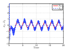
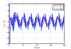
Figure 1: Estimation of $(x_{2}(t),x_{3}(t))$ by the linear event-triggered ESO.

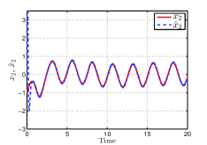
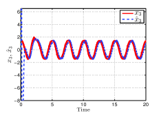
Figure 2: Estimation of $(x_{2}(t),x_{3}(t))$ by the nonlinear event-triggered ESO.

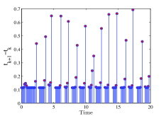
(a) Corresponding to ETM (12)

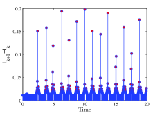
(b) Corresponding to ETM (20)

Figure 3: Inter-execution times corresponding to ETMs (12) and (20) for respective linear and nonlinear event-triggered ESOs.

V Concluding remarks

This paper investigates both the linear and nonlinear event-triggered extended state observers (ESOs) for a class of uncertain stochastic systems driven by bounded and colored noises. Two event-triggering mechanisms with dwell time are proposed for the designs of the event-triggered ESOs, which guarantee a positive minimum inter-event time for every sample path solution of the stochastic systems to avoid directly the Zeno phenomenon. Not only the mean square convergence but also the almost sure one of the estimation errors of unmeasured state and stochastic total disturbance are given with rigorous theoretical proofs. The theoretical results also show that the nonlinear event-triggered ESO has higher estimation accuracy but higher triggering frequency than the linear one. A successive interesting problem to be further developed could be the event-triggered active disturbance rejection control (ADRC) for the uncertain stochastic systems based on the event-triggered ESOs.

APPENDIX A: Proof of Theorem III.1

Define error variables as follows: $\eta_{i}(t)=r^{n+1-i}(x_{i}(t)-\hat{x}_{i}(t))\;(i=1,\cdots,n+1)$, $\eta(t)=(\eta_{1}(t),\cdots,\eta_{n+1}(t))$. For any fixed $t\in[0,\infty)$, the last execution time before $t$ can be expressed as $\varrho_{t}=\max\{t_{k}:t_{k}\leq t,k\in\mathbb{Z}^{+}\}$. Therefore, $y(t_{k})-y(t),\;t\in[t_{k},t_{k+1})$ can be expressed as $y(\varrho_{t})-y(t)$. Set $\kappa(t)=r^{n}(y(\varrho_{t})-y(t))$. Since $t_{k+1}-t_{k}\geq\tau$, for almost every sample path, there are at most $[\frac{t}{\tau}]+1$ execution times before $t$. Define $\Omega_{k}=\{\varrho_{t}=t_{k}\},\;\Omega_{k,\tau}=\{\varrho_{t}=t_{k}\;\mbox{and}\;t\leq t_{k}+\tau\},k=1,\cdots,[\frac{t}{\tau}]+1$. It can be obtained that $\Omega$ can be expressed as the union of a set of mutually disjoint subset as $\Omega=\bigcup^{[\frac{t}{\tau}]+1}_{k=1}\Omega_{k}$ for each $t\in[0,\infty)$. Applying Itô’s formula to $f(t,x(t),v_{1}(t),v_{2}(t))$ with respect to $t$ along system (9) and (10), it is obtained that

$$dx_{n+1}(t)=\frac{\partial f(t,x(t),v_{1}(t),v_{2}(t))}{\partial t}dt$$ (25)

$$+\sum\limits^{n-1}_{i=1}\frac{\partial f(t,x(t),v_{1}(t),v_{2}(t))}{\partial x_{i}}x_{i+1}(t)dt$$ (26)

$$+\frac{\partial f(t,x(t),v_{1}(t),v_{2}(t))}{\partial x_{n}}[f(t,x(t),v_{1}(t),v_{2}(t))+u(t)]dt$$ (27)

$$+\frac{\partial f(t,x(t),v_{1}(t),v_{2}(t))}{\partial v_{1}}[\frac{\partial\sigma(t,B_{1}(t))}{\partial t}+\frac{1}{2}\frac{\partial^{2}\sigma(t,B_{1}(t))}{\partial\varsigma^{2}}]dt$$ (28)

$$+\frac{1}{2}\frac{\partial^{2}f(t,x(t),v_{1}(t),v_{2}(t))}{\partial v^{2}_{1}}(\frac{\partial\sigma(t,B_{1}(t))}{\partial\varsigma})^{2}dt$$ (29)

$$-\frac{\partial f(t,x(t),v_{1}(t),v_{2}(t))}{\partial v_{2}}\alpha_{1}v_{2}(t)dt$$ (30)

$$+\frac{\partial^{2}f(t,x(t),v_{1}(t),v_{2}(t))}{\partial v^{2}_{2}}\alpha^{2}_{1}\alpha_{2}dt$$ (31)

$$+\frac{\partial f(t,x(t),v_{1}(t),v_{2}(t))}{\partial v_{1}}\frac{\partial\sigma(t,B_{1}(t))}{\partial\varsigma}dB_{1}(t)$$ (32)

$$+\frac{\partial f(t,x(t),v_{1}(t),v_{2}(t))}{\partial v_{2}}\alpha_{1}\sqrt{2\alpha_{2}}dB_{2}(t)$$ (33)

$$=:\Delta_{1}(t)dt+\Delta_{2}(t)dB_{1}(t)+\Delta_{3}(t)dB_{2}(t),$$ (34)

where $\varsigma$ represents the second argument of the function $\sigma(\cdot,\cdot)$. By Assumptions (A1)-(A3) and the mean square boundedness of the colored noise $v_{2}(t)$, there exist known positive constants $C_{1}$ and $C_{2}$ such that

$$\sup_{t\geq 0}\mathbb{E}[|\Delta_{1}(t)|^{2}+|\Delta_{2}(t)|^{2}]\leq C_{1},\;\sup_{t\geq 0}|\Delta_{3}(t)|^{2}\leq C_{2}.$$ (35)

A direct computation shows that the error variable $\eta(t)$ satisfies the following Itô-type stochastic differential equation

$$\left\{\begin{array}[]{l}d\eta_{1}(t)=r[\eta_{2}(t)-a_{1}\eta_{1}(t)]dt-a_{1}r\kappa(t)dt,\cr d\eta_{2}(t)=r[\eta_{3}(t)-a_{2}\eta_{1}(t)]dt-a_{2}r\kappa(t)dt,\cr\hskip 34.14322pt\vdots\cr d\eta_{n}(t)=r[\eta_{n+1}(t)-a_{n}\eta_{1}(t)]dt-a_{n}r\kappa(t)dt,\cr d\eta_{n+1}(t)=-ra_{n+1}\eta_{1}(t)dt-a_{n+1}r\kappa(t)dt+\Delta_{1}(t)dt\cr\hskip 51.21504pt+\Delta_{2}(t)dB_{1}(t)+\Delta_{3}(t)dB_{2}(t).\end{array}\right.$$ (42)

Define the Lyapunov function $V:\mathbb{R}^{n+1}\rightarrow\mathbb{R}$ by $V(\eta)=\eta Q\eta^{\top}$ for $\eta\in\mathbb{R}^{n+1}$.

Apply Itô’s formula to $V(\eta(t))$ with respect to $t$ along system (42), and by (35) and Young’s inequality, for any $r\geq r^{*}$, it can be obtained that

$$\frac{d\mathbb{E}V(\eta(t))}{dt}$$ (43)

$$\leq-r\mathbb{E}\|\eta(t)\|^{2}+2r\lambda_{\max}(Q)\sum^{n+1}_{i=1}|a_{i}|\sum^{[\frac{t}{\tau}]+1}_{k=1}\mathbb{E}(\|\eta(t)\||\kappa(t)|\mathbb{I}_{\Omega_{k}})$$ (44)

$$+\lambda^{2}_{\max}(Q)\mathbb{E}\|\eta(t)\|^{2}+C_{1}+\lambda_{\max}(Q)(C_{1}+C_{2})$$ (45)

$$\leq-\xi_{0}r\mathbb{E}V(\eta(t))+\mu_{0}r\sum^{[\frac{t}{\tau}]+1}_{k=1}\mathbb{E}[\kappa^{2}(t)\mathbb{I}_{\Omega_{k}}]+C_{1}$$ (46)

$$+\lambda_{\max}(Q)(C_{1}+C_{2}),$$ (47)

where $\mu_{0}>0$ is chosen such that $\xi_{0}:=\frac{1-\zeta}{\lambda_{\max}(Q)}-\frac{\lambda_{\max}(Q)(\sum^{n+1}_{i=1}|a_{i}|)^{2}}{\mu_{0}}>0.$ By the triggering mechanism (12), we have $\sum^{[\frac{t}{\tau}]+1}_{k=1}\mathbb{E}[\kappa^{2}(t)\mathbb{I}_{\Omega_{k}\setminus\Omega_{k,\tau}}]\leq\frac{\theta^{2}}{r},\;\forall t\geq 0.$ It follows from Assumption (A3) and $\tau=\epsilon r^{-(n+\frac{1}{2})}$ that

$$\sum^{[\frac{t}{\tau}]+1}_{k=1}\mathbb{E}[\kappa^{2}(t)\mathbb{I}_{\Omega_{k,\tau}}]=r^{2n}\sum^{[\frac{t}{\tau}]+1}_{k=1}\mathbb{E}\left[\left(\int^{t}_{t_{k}}x_{2}(s)ds\right)^{2}\mathbb{I}_{\Omega_{k,\tau}}\right]$$ (48)

$$\leq r^{2n}\tau\int^{t}_{t-\tau}\mathbb{E}x^{2}_{2}(s)ds\leq\frac{M\epsilon^{2}}{r},\;\forall t\geq\tau,$$ (49)

and it can be easily obtained that $\mathbb{E}[\kappa^{2}(t)\mathbb{I}_{\Omega_{1,\tau}}]\leq\frac{M\epsilon^{2}}{r}$ also holds for $t\in[0,\tau)$ where $\varrho_{t}=0$ a.s. For any $t\in[T,\infty)$, it holds that $e^{-\xi_{0}rt}\mathbb{E}V(\eta(0))\leq\lambda_{\max}(Q)e^{-\xi_{0}rT}\sum^{n+1}_{i=1}r^{2(n+1-i)}\mathbb{E}|x_{i}(0)-\hat{x}_{i}(0)|^{2}\leq\frac{\Theta_{1}}{r}$, for some $r$-independent constant $\Theta_{1}:=\sup_{r\geq r^{*}}\lambda_{\max}(Q)e^{-\xi_{0}rT}\sum^{n+1}_{i=1}r^{2n+3-2i}\mathbb{E}|x_{i}(0)-\hat{x}_{i}(0)|^{2}$ which is finite since $\lim_{r\rightarrow\infty}e^{-\xi_{0}rT}\sum^{n+1}_{i=1}r^{2n+3-2i}=0$. Thus, for any $r\geq r^{*}$ and $t\in[T,\infty)$, we have

$$\mathbb{E}V(\eta(t))$$

$$\leq e^{-\xi_{0}rt}\mathbb{E}V(\eta(0))+\mu_{0}r\int^{t}_{0}e^{-\xi_{0}r(t-s)}\sum^{[\frac{s}{\tau}]+1}_{k=1}\bigg{\{}\mathbb{E}[\kappa^{2}(s)\mathbb{I}_{\Omega_{k,\tau}}]$$

$$+\mathbb{E}[\kappa^{2}(s)\mathbb{I}_{\Omega_{k}\setminus\Omega_{k,\tau}}]\bigg{\}}ds+\frac{C_{1}+\lambda_{\max}(Q)(C_{1}+C_{2})}{\xi_{0}r}\leq\frac{\Theta_{2}}{r},$$

where $\Theta_{2}:=\Theta_{1}+\frac{\mu_{0}(\theta^{2}+M\epsilon^{2})}{\xi_{0}}+\frac{C_{1}+\lambda_{\max}(Q)(C_{1}+C_{2})}{\xi_{0}}$. This further yields that, for all $i=1,\cdots,n+1$,

$$\mathbb{E}|x_{i}(t)-\hat{x}_{i}(t)|^{2}\leq\frac{1}{r^{2n+2-2i}}\mathbb{E}|\eta_{i}(t)|^{2}$$ (50)

$$\leq\frac{1}{\lambda_{\min}(Q)r^{2n+2-2i}}\mathbb{E}V(\eta(t))\leq\frac{\Theta}{r^{2n+3-2i}},$$ (51)

uniformly in $t\in[T,\infty)$, where $\Theta:=\frac{\Theta_{2}}{\lambda_{\min}(Q)}$. In addition, by (50) and Chebyshev’s inequality ([15, p.5]), it holds that $P\{|x_{i}(t)-\hat{x}_{i}(t)|\geq m\sqrt{\Theta}(\frac{1}{r})^{\frac{2n+3-2i}{2}}\}\leq\frac{1}{m^{2}}$ uniformly in $t\in[T,\infty)$ and for $m\in\mathbb{Z}^{+}$. From the Borel-Cantelli’s lemma ([15, p.7]), for almost all $\omega\in\Omega$, there exists a random variable $m^{*}(\omega)$ such that whenever $m\geq m^{*}(\omega)$, we have

$$|x_{i}(t)-\hat{x}_{i}(t)|\leq\frac{m\sqrt{\Theta}}{r^{n+\frac{3}{2}-i}},\;t\in[T,\infty).$$ (52)

Set $\Theta_{\omega}=m^{*}(\omega)\sqrt{\Theta}>0$ which is an $r$-independent random variable. This completes the proof.

APPENDIX B: Proof of Theorem III.2

The following $\eta(t)$, $\varrho_{t}$ and $\kappa(t)$ are defined as those in Appendix A. Similarly, for almost every sample path, there are at most $[\frac{t}{\tau^{*}}]+1$ execution times before $t$. Define $\Omega^{*}_{k}=\{\varrho_{t}=t_{k}\},\;\Omega^{*}_{k,\tau^{*}}=\{\varrho_{t}=t_{k}\;\mbox{and}\;t\leq t_{k}+\tau^{*}\},k=1,\cdots,[\frac{t}{\tau^{*}}]+1$, and then $\Omega=\bigcup^{[\frac{t}{\tau^{*}}]+1}_{k=1}\Omega^{*}_{k}$ for each $t\in[0,\infty)$. By simple analysis, it can be easily obtained that $|\langle\theta_{1}\rangle^{\vartheta}-\langle\theta_{2}\rangle^{\vartheta}|\leq 2^{1-\vartheta}|\theta_{1}-\theta_{2}|^{\vartheta}$ for all $\theta_{1},\theta_{2}\in\mathbb{R}$ and $\vartheta\in(0,1)$. For $i=1,\cdots,n+1$, we set $\delta_{i}(t)=\langle\eta_{1}(t)\rangle^{i\nu-(i-1)}-\langle\eta_{1}(t)+\kappa(t)\rangle^{i\nu-(i-1)}$. It then follows that $|\delta_{i}(t)|\leq 2^{i(1-\nu)}|\kappa(t)|^{i\nu-(i-1)},\;\forall t\geq 0$.

A direct computation shows that the error variable $\eta(t)$ satisfies the following Itô-type stochastic differential equation

$$\left\{\begin{array}[]{l}d\eta_{1}(t)=[r(\eta_{2}(t)-a_{1}\langle\eta_{1}(t)\rangle^{\nu})+a_{1}r\delta_{1}(t)]dt,\cr d\eta_{2}(t)=[r(\eta_{3}(t)-a_{2}\langle\eta_{1}(t)\rangle^{2\nu-1})+a_{2}r\delta_{2}(t)]dt,\cr\hskip 34.14322pt\vdots\cr d\eta_{n}(t)=[r(\eta_{n+1}(t)-a_{n}\langle\eta_{1}(t)\rangle^{n\nu-(n-1)})+a_{n}r\delta_{n}(t)]dt,\cr d\eta_{n+1}(t)=-ra_{n+1}\langle\eta_{1}(t)\rangle^{(n+1)\nu-n}dt+a_{n+1}r\delta_{n+1}(t)dt\cr\hskip 51.21504pt+\Delta_{1}(t)dt+\Delta_{2}(t)dB_{1}(t)+\Delta_{3}(t)dB_{2}(t),\end{array}\right.$$ (53)

where $\Delta_{i}(t)\;(i=1,2,3)$ are defined as those in (25) satisfying (35). As a consequence of Lemmas II.3-II.4, system $\dot{\eta}(t)=\Phi(\eta(t))$ is globally finite-time stable, where $\Phi(\cdot)$ is defined in (2). Using Lemma II.1, for any $\mu$ satisfying $\displaystyle\max\{1,2w_{n+1}\}<\mu<d_{0}+2w_{n+1}$ with $d_{0}:=1-\nu>0$, we can conclude that there exists a positive definite, radially unbounded function $V\in C^{1}(\mathbb{R}^{n+1};\mathbb{R})\cap C^{\infty}(\mathbb{R}^{n+1}\setminus\{0_{n+1}\};\mathbb{R})\$ such that $V$ is homogeneous of degree $\mu$ with respect to weights $\{w_{l}=(l-1)\nu-(l-2)\}_{l=1}^{n+1}$, and the Lie derivative of $V(\eta)$ along the vector field $\Phi$:

$$L_{\Phi}V(\eta):=\sum^{n+1}_{i=1}\frac{\partial V(\eta)}{\partial\eta_{i}}\Phi_{i}(\eta)=\sum_{i=1}^{n}\dfrac{\partial V(\eta)}{\partial\eta_{i}}\left(\eta_{i+1}\right.$$ (54)

$$\left.-a_{i}\langle\eta_{1}\rangle^{i\nu-(i-1)}\right)-\dfrac{\partial V(\eta)}{\partial\eta_{n+1}}a_{n+1}\langle\eta_{1}\rangle^{(n+1)\nu-n}$$ (55)

is negative definite. By the definition of homogeneity in Definition 2 and the fact that $V(\eta)$ is homogeneous of degree $\mu$ with respect to weights $\{w_{l}\}_{l=1}^{n+1}$, it can be easily obtained that $L_{\Phi}V(\eta)$, $\dfrac{\partial V(\eta_{1},\cdots,\eta_{n+1})}{\partial\eta_{i}}$, $\dfrac{\partial^{2}V(\eta_{1},\cdots,\eta_{n+1})}{\partial\eta^{2}_{n+1}}$ and $|\eta_{i}|$ are homogeneous of degree $\mu-d_{0}$, $\mu-w_{i}$, $\mu-2w_{n+1}$ and $w_{i}$ with respect to weights $\{w_{l}\}_{l=1}^{n+1}$, respectively. The above analysis together with Lemma II.2 yields the following inequalities:

$$L_{\Phi}V(\eta)\leq-c_{1}(V(\eta))^{\frac{\mu-d_{0}}{\mu}},|\dfrac{\partial V(\eta)}{\partial\eta_{i}}|\leq c_{2i}(V(\eta))^{\frac{\mu-w_{i}}{\mu}},$$ (56)

$$|\eta_{i}|\leq c_{3i}(V(\eta))^{\frac{w_{i}}{\mu}},\;\forall\eta\in\mathbb{R}^{n+1},$$ (57)

$$|\dfrac{\partial^{2}V(\eta)}{\partial\eta^{2}_{n+1}}|\leq c_{4}(V(\eta))^{\frac{\mu-2w_{n+1}}{\mu}},\forall\eta\in\mathbb{R}^{n+1}\setminus\{0_{n+1}\},$$ (58)

for some positive constants $c_{1},c_{2i},c_{3i},c_{4}$. For any fixed $t\in[0,\infty)$, the transient convergence result (23) holds directly for $\omega\in\Omega_{t}:=\{\|\eta(t)\|=0\}$, so we only need to analyze $\mathcal{L}V(\eta(t))$ for $\omega\in\Omega\setminus\Omega_{t}$. It follows from (56) that $|\dfrac{\partial^{2}V(\eta(t))}{\partial\eta^{2}_{n+1}}|\leq c_{4}(V(\eta(t)))^{\frac{\mu-2w_{n+1}}{\mu}}$, for $\omega\in\Omega\setminus\Omega_{t}$. For convenience of the symbol, we proceed the proof by assuming that this inequality holds for almost all $\omega\in\Omega$ without loss of generality. Since $\nu>1-\frac{1}{n+1}$, $\frac{\mu-w_{n+1}}{\mu}<\frac{\mu-d_{0}}{\mu}$. These together with the inequalities used repeatedly hereinbelow: $ab\leq\frac{1}{p_{0}}a^{p_{0}}+\frac{1}{q_{0}}b^{q_{0}}$ and $(\sum^{m}_{i=1}a_{i})^{\vartheta}\leq m^{\vartheta-1}\sum^{m}_{i=1}a^{\vartheta}_{i}$ with $\vartheta,p_{0},q_{0}>1$, $\frac{1}{p_{0}}+\frac{1}{q_{0}}=1$, $m\in\mathbb{Z}^{+}$, $a,b,a_{i}\geq 0$, yield that

$$\mathcal{L}V(\eta(t))$$

$$=rL_{\Phi}V(\eta(t))+r\sum^{n+1}_{i=1}\dfrac{\partial V(\eta(t))}{\partial\eta_{i}}a_{i}\delta_{i}(t)+\dfrac{\partial V(\eta(t))}{\partial\eta_{n+1}}\Delta_{1}(t)$$

$$+\frac{1}{2}\dfrac{\partial^{2}V(\eta(t))}{\partial\eta^{2}_{n+1}}(\Delta^{2}_{2}(t)+\Delta^{2}_{3}(t))$$

$$\leq-c_{1}r(V(\eta(t)))^{\frac{\mu-d_{0}}{\mu}}+\sum^{n+1}_{i=1}(a_{i}c_{2i}2^{(1-\nu)i})^{\frac{\mu-d_{0}}{\mu-w_{i}}}\frac{\mu-w_{i}}{\mu-d_{0}}\cdot$$

$$(V(\eta(t)))^{\frac{\mu-d_{0}}{\mu}}+\sum^{n+1}_{i=1}\sum^{[\frac{t}{\tau^{*}}]+1}_{k=1}r^{\frac{\mu-d_{0}}{w_{i}-d_{0}}}\frac{w_{i}-d_{0}}{\mu-d_{0}}\{|\kappa(t)|^{\frac{w_{i+1}(\mu-d_{0})}{w_{i}-d_{0}}}$$

$$\mathbb{I}_{\Omega^{*}_{k}}\}+\frac{c_{2(n+1)}(\mu-w_{n+1})}{\mu-d_{0}}(V(\eta(t)))^{\frac{\mu-d_{0}}{\mu}}+c_{2(n+1)}\cdot$$

$$\frac{(w_{n+1}-d_{0})}{\mu-d_{0}}|\Delta_{1}(t)|^{\frac{\mu-d_{0}}{w_{n+1}-d_{0}}}+\frac{c_{4}(\mu-2w_{n+1})}{2(\mu-d_{0})}(V(\eta(t)))^{\frac{\mu-d_{0}}{\mu}}$$

$$+\frac{c_{4}(2w_{n+1}-d_{0})}{2(\mu-d_{0})}2^{\frac{\mu-2w_{n+1}}{2w_{n+1}-d_{0}}}[|\Delta_{2}(t)|^{\frac{2(\mu-d_{0})}{2w_{n+1}-d_{0}}}+C^{\frac{\mu-d_{0}}{2w_{n+1}-d_{0}}}_{2}],$$

where $w_{n+2}:=(n+1)\nu-n$. Choose $r_{0}>0$ such that $\frac{c_{1}r_{0}}{2}-\sum^{n+1}_{i=1}(a_{i}c_{2i}2^{(1-\nu)i})^{\frac{\mu-d_{0}}{\mu-w_{i}}}\frac{\mu-w_{i}}{\mu-d_{0}}-\frac{c_{2(n+1)}(\mu-w_{n+1})}{\mu-d_{0}}-\frac{c_{4}(\mu-2w_{n+1})}{2(\mu-d_{0})}>0$. Then, for any $r\geq r^{*}:=\max\{1,r_{0}\}$ and any $t\geq 0$, it holds that

$$\mathcal{L}V(\eta(t))\leq-\frac{c_{1}r}{2}(V(\eta(t)))^{\frac{\mu-d_{0}}{\mu}}+\Gamma_{1}+\sum^{4}_{i=2}\Gamma_{i}(t),$$ (59)

where we set

$$\Gamma_{1}=\frac{c_{4}(2w_{n+1}-d_{0})}{2(\mu-d_{0})}2^{\frac{\mu-2w_{n+1}}{2w_{n+1}-d_{0}}}C^{\frac{\mu-d_{0}}{2w_{n+1}-d_{0}}}_{2},$$ (60)

$$\Gamma_{2}(t)=\sum^{n+1}_{i=1}\sum^{[\frac{t}{\tau^{*}}]+1}_{k=1}r^{\frac{\mu-d_{0}}{w_{i}-d_{0}}}\frac{w_{i}-d_{0}}{\mu-d_{0}}\{|\kappa(t)|^{\frac{w_{i+1}(\mu-d_{0})}{w_{i}-d_{0}}}\mathbb{I}_{\Omega^{*}_{k}}\},$$ (61)

$$\Gamma_{3}(t)=\frac{c_{2(n+1)}(w_{n+1}-d_{0})}{\mu-d_{0}}|\Delta_{1}(t)|^{\frac{\mu-d_{0}}{w_{n+1}-d_{0}}},$$ (62)

$$\Gamma_{4}(t)=\frac{c_{4}(2w_{n+1}-d_{0})}{2(\mu-d_{0})}2^{\frac{\mu-2w_{n+1}}{2w_{n+1}-d_{0}}}|\Delta_{2}(t)|^{\frac{2(\mu-d_{0})}{2w_{n+1}-d_{0}}}.$$ (63)

Define the stopping time as follows:

$$\varpi=\inf\{t\geq 0:V(\eta(t))\leq[\frac{4}{c_{1}r}(\Gamma_{1}+\sum^{4}_{i=2}\Gamma_{i}(t))]^{\frac{\mu}{\mu-d_{0}}}\}.$$

If $V(\eta(t))\geq[\frac{4}{c_{1}r}(\Gamma_{1}+\sum^{4}_{i=2}\Gamma_{i}(t))]^{\frac{\mu}{\mu-d_{0}}}$ for some $t>\varpi$, then $\frac{d\mathbb{E}V(\eta(t))}{dt}=\mathbb{E}\mathcal{L}V(\eta(t))\leq 0$. Thus, $\mathbb{E}V(\eta(t))\leq\mathbb{E}[\frac{4}{c_{1}r}(\Gamma_{1}+\sum^{4}_{i=2}\Gamma_{i}(t))]^{\frac{\mu}{\mu-d_{0}}}$ for all $t\in[\varpi,\infty)$. Therefore, for all $i=1,\cdots,n+1$ and $t\in[\varpi,\infty)$, it follows from (56) and Hölder’s inequality that

$$\mathbb{E}|x_{i}(t)-\hat{x}_{i}(t)|=\frac{1}{r^{n+1-i}}\mathbb{E}|\eta_{i}(t)|\leq\frac{c_{3i}}{r^{n+1-i}}\mathbb{E}(V(\eta(t)))^{\frac{w_{i}}{\mu}}$$ (64)

$$\leq\frac{c_{3i}}{r^{n+1-i}}(\mathbb{E}(V(\eta(t)))^{\frac{w_{i}}{\mu}}\leq(\frac{1}{r})^{n+1+\frac{w_{i}}{\mu-d_{0}}-i}c_{3i}(\frac{4}{c_{1}})^{\frac{w_{i}}{\mu-d_{0}}}$$ (65)

$$\times 4^{\frac{d_{0}w_{i}}{(\mu-d_{0})\mu}}\left[\Gamma_{1}^{\frac{\mu}{\mu-d_{0}}}+\sum^{4}_{i=2}\mathbb{E}[\Gamma_{i}(t)]^{\frac{\mu}{\mu-d_{0}}}\right]^{\frac{w_{i}}{\mu}}.$$ (66)

By $\tau^{*}=\epsilon^{*}r^{-(n+\frac{1}{w_{n+1}})}$ and Assumption (A4), we have

$$\mathbb{E}\{\sum^{n+1}_{i=1}\sum^{[\frac{t}{\tau^{*}}]+1}_{k=1}r^{\frac{\mu-d_{0}}{w_{i}-d_{0}}}\frac{w_{i}-d_{0}}{\mu-d_{0}}[|\kappa(t)|^{\frac{w_{i+1}(\mu-d_{0})}{w_{i}-d_{0}}}\mathbb{I}_{\Omega^{*}_{k,\tau}}]\}^{\frac{\mu}{\mu-d_{0}}}$$ (67)

$$\leq(n+1)^{\frac{d_{0}}{\mu-d_{0}}}\sum^{n+1}_{i=1}\sum^{[\frac{t}{\tau^{*}}]+1}_{k=1}r^{(1+nw_{i+1})\frac{\mu}{w_{i}-d_{0}}}(\frac{w_{i}-d_{0}}{\mu-d_{0}})^{\frac{\mu}{\mu-d_{0}}}$$ (68)

$$\times\mathbb{E}((\int^{t}_{t_{k}}|x_{2}(s)|ds)^{\frac{w_{i+1}\mu}{w_{i}-d_{0}}}\mathbb{I}_{\Omega^{*}_{k,\tau}})$$ (69)

$$\leq(n+1)^{\frac{d_{0}}{\mu-d_{0}}}\sum^{n+1}_{i=1}r^{(1+nw_{i+1})\frac{\mu}{w_{i}-d_{0}}}(\frac{w_{i}-d_{0}}{\mu-d_{0}})^{\frac{\mu}{\mu-d_{0}}}$$ (70)

$$\times(\int^{t}_{t-\tau^{*}}\mathbb{E}|x_{2}(s)|^{p}ds)^{\frac{w_{i+1}\mu}{p(w_{i}-d_{0})}}\tau^{*\frac{w_{i+1}\mu}{q(w_{i}-d_{0})}}$$ (71)

$$\leq(n+1)^{\frac{d_{0}}{\mu-d_{0}}}\sum^{n+1}_{i=1}r^{(1+nw_{i+1})\frac{\mu}{w_{i}-d_{0}}}(\frac{w_{i}-d_{0}}{\mu-d_{0}})^{\frac{\mu}{\mu-d_{0}}}$$ (72)

$$\times N^{\frac{w_{i+1}\mu}{p(w_{i}-d_{0})}}\tau^{*\frac{w_{i+1}\mu}{w_{i}-d_{0}}}\leq M_{1},\;\forall t\geq\tau^{*},$$ (73)

where $M_{1}=(n+1)^{\frac{d_{0}}{\mu-d_{0}}}\sum^{n+1}_{i=1}(\frac{w_{i}-d_{0}}{\mu-d_{0}})^{\frac{\mu}{\mu-d_{0}}}N^{\frac{w_{i+1}\mu}{p(w_{i}-d_{0})}}\epsilon^{*\frac{w_{i+1}\mu}{w_{i}-d_{0}}}$ and $q$ satisfies $\frac{1}{p}+\frac{1}{q}=1$, and it follows easily that the inequality (67) also holds for $t\in[0,\tau^{*})$ where $\varrho_{t}=0$ a.s. By the event-triggering mechanism (20), for all $t\geq 0$, it holds that

$$\mathbb{E}\{\sum^{n+1}_{i=1}\sum^{[\frac{t}{\tau^{*}}]+1}_{k=1}r^{\frac{\mu-d_{0}}{w_{i}-d_{0}}}\frac{w_{i}-d_{0}}{\mu-d_{0}}[|\kappa(t)|^{\frac{w_{i+1}(\mu-d_{0})}{w_{i}-d_{0}}}\mathbb{I}_{\Omega^{*}_{k}\setminus\Omega^{*}_{k,\tau}}]\}^{\frac{\mu}{\mu-d_{0}}}$$ (74)

$$\displaystyle\leq M_{2},$$ (75)

where $M_{2}:=(n+1)^{\frac{d_{0}}{\mu-d_{0}}}\sum^{n+1}_{i=1}\theta^{*\frac{w_{i+1}\mu}{w_{i}-d_{0}}}(\frac{w_{i}-d_{0}}{\mu-d_{0}})^{\frac{\mu}{\mu-d_{0}}}.$ Thus, it follows from (67) and (74) that

$$\mathbb{E}[\Gamma_{2}(t)]^{\frac{\mu}{\mu-d_{0}}}\leq 2^{\frac{d_{0}}{\mu-d_{0}}}(M_{1}+M_{2}),\;\forall t\geq 0.$$ (76)

By $\nu>1-\frac{p-2}{(p-2)n+p+1}$ and $\mu<d_{0}+2w_{n+1}$, it follows that $\frac{\mu}{w_{n+1}-d_{0}}<p$. Thus, it follows from Assumptions (A1), (A2) and (A4) that for all $t\geq 0$,

$$\mathbb{E}[\Gamma_{3}(t)]^{\frac{\mu}{\mu-d_{0}}}\leq[\frac{c_{2(n+1)}(w_{n+1}-d_{0})}{\mu-d_{0}}]^{\frac{\mu}{\mu-d_{0}}}\mathbb{E}|\Delta_{1}(t)|^{p}\leq M_{3}$$

for some $M_{3}>0$. Similarly, we also have $\frac{2\mu}{2w_{n+1}-d_{0}}<p$. Then, it follows from Assumptions (A1), (A2) and (A4) that for all $t\geq 0$,

$$\mathbb{E}[\Gamma_{4}(t)]^{\frac{\mu}{\mu-d_{0}}}\leq[\frac{c_{4}(2w_{n+1}-d_{0})}{2(\mu-d_{0})}2^{\frac{\mu-2w_{n+1}}{2w_{n+1}-d_{0}}}]^{\frac{\mu}{\mu-d_{0}}}\mathbb{E}|\Delta_{2}(t)|^{p}$$

$$\hskip 39.83368pt\leq M_{4}$$

for some $M_{4}>0$. These together with (64), yield that for all $i=1,\cdots,n+1$ and $t\in[\varpi,\infty)$,

$$\mathbb{E}|x_{i}(t)-\hat{x}_{i}(t)|\leq\Xi_{i}\cdot(\frac{1}{r})^{n+1+\frac{w_{i}}{\mu-d_{0}}-i},$$ (77)

where we set $\Xi_{i}=c_{3i}(\frac{4}{c_{1}})^{\frac{w_{i}}{\mu-d_{0}}}4^{\frac{d_{0}w_{i}}{(\mu-d_{0})\mu}}[\Gamma_{1}^{\frac{\mu}{\mu-d_{0}}}+2^{\frac{d_{0}}{\mu-d_{0}}}(M_{1}+M_{2})+M_{3}+M_{4}]^{\frac{w_{i}}{\mu}}$. In addition, by Chebyshev’s inequality ([15, p.5]), it holds that $P\{|x_{i}(t)-\hat{x}_{i}(t)|\geq m^{2}\Xi_{i}\cdot(\frac{1}{r})^{n+1+\frac{w_{i}}{\mu-d_{0}}-i}\}\leq\frac{1}{m^{2}}$ for all $m\in\mathbb{Z}^{+}$, $i=1,\cdots,n+1$ and $t\in[\varpi,\infty)$. From the Borel-Cantelli’s lemma ([15, p.7]), for almost all $\omega\in\Omega$ and $t\in[\varpi,\infty)$, there exists a random variable $m_{0}(\omega)$ such that whenever $m\geq m_{0}(\omega)$, we have

$$|x_{i}(t)-\hat{x}_{i}(t)|\leq m^{2}\Xi_{i}\cdot(\frac{1}{r})^{n+1+\frac{w_{i}}{\mu-d_{0}}-i}.$$ (78)

Then (23) is obtained by letting $\Xi_{i,\omega}=m^{2}_{0}(\omega)\Xi_{i}>0$ which is a random variable independent of $r$. Next we prove $\mathbb{E}\varpi\leq T_{r}$ for some $r$-dependent positive constant $T_{r}$. Define a series of stopping times as follows:

$$\varpi_{m}=\inf\{t\geq 0:V(\eta(t))\leq[\frac{4}{c_{1}r}(\Gamma_{1}+\sum^{4}_{i=2}\Gamma_{i}(t))]^{\frac{\mu}{\mu-d_{0}}}+\frac{1}{m}$$

$$\mbox{or}\;V(\eta(t))\geq[\frac{4}{c_{1}r}(\Gamma_{1}+\sum^{4}_{i=2}\Gamma_{i}(t))]^{\frac{\mu}{\mu-d_{0}}}+m\},\;m\in\mathbb{Z}^{+}.$$

Set $\Upsilon(V)=\frac{4}{c_{1}r}\int^{V}_{0}\vartheta^{-\frac{\mu-d_{0}}{\mu}}d\vartheta,\;V\in[0,\infty)$. Thus, for all $t\in[0,\varpi_{m})$, it holds that

$$\mathcal{L}\Upsilon(V(\eta(t)))$$ (79)

$$=\frac{4}{c_{1}r}(V(\eta(t)))^{-\frac{\mu-d_{0}}{\mu}}\mathcal{L}V(\eta(t))-\frac{2(\mu-d_{0})}{c_{1}r\mu}(V(\eta(t)))^{-\frac{2\mu-d_{0}}{\mu}}$$ (80)

$$\times[(\frac{\partial V(\eta(t))}{\partial\eta_{n+1}}\Delta_{2}(t))^{2}+(\frac{\partial V(\eta(t))}{\partial\eta_{n+1}}\Delta_{3}(t))^{2}]\leq-1.$$ (81)

Set $t_{m}=m\wedge\varpi_{m}$ for $m\in\mathbb{Z}^{+}$. Then

$$\mathbb{E}[\Upsilon(V(\eta(t_{m})))]-\mathbb{E}[\Upsilon(V(\eta(0)))]$$ (82)

$$=\mathbb{E}\int^{t_{m}}_{0}\mathcal{L}\Upsilon(V(\eta(s)))ds\leq-\mathbb{E}[t_{m}]$$ (83)

which means that $\mathbb{E}[t_{m}]\leq\mathbb{E}[\Upsilon(V(\eta(0)))]$. Passing to the limit as $m\rightarrow\infty$ and using the Fatou’s lemma, we obtain $\mathbb{E}\varpi\leq\frac{4\mu}{c_{1}d_{0}r}\mathbb{E}[V(\eta(0))]^{\frac{d_{0}}{\mu}}=:T_{r}<\infty$. This completes the proof.

References

- [1] J. Han, From PID to active disturbance rejection control, IEEE Trans. Ind. Electron. 56 (2009) 900-906.
- [2] B. Guo, Z. Zhao, On the convergence of an extended state observer for nonlinear systems with uncertainty, Syst. Control Lett. 60 (2011) 420-430.
- [3] Z. Zhao, B. Guo, A nonlinear extended state observer based on fractional power functions, Automatica 81 (2017) 286-296.
- [4] B. Guo, Z. Wu, H. Zhou, Active disturbance rejection control approach to output-feedback stabilization of a class of uncertain nonlinear systems subject to stochastic disturbance, IEEE Trans. Autom. Control 61 (2015) 1613-1618.
- [5] Z. Wu, B. Guo, Extended state observer for MIMO nonlinear systems with stochastic uncertainties, Int. J. Control. 93 (2020) 424-436.
- [6] Y. Huang, J. Wang, D. Shi, L. Shi, Toward event-triggered extended state observer, IEEE Trans. Autom. Control 63 (2017) 1842-1849.
- [7] F. Li, Y. Liu, Event-triggered stabilization for continuous-time stochastic systems, IEEE Trans. Autom. Control 65 (2019) 4031-4046.
- [8] S. Luo, F. Deng, On event-triggered control of nonlinear stochastic systems, IEEE Trans. Autom. Control 65 (2019) 369-375.
- [9] F. Li, Y. Liu, An enlarged framework of event-triggered control for stochastic systems, IEEE Trans. Autom. Control 66 (2020) 4132-4147.
- [10] W. Perruquetti, T. Floquet, E. Moulay, Finite-time observers: application to secure communication, IEEE Trans. Autom. Control 53 (2008) 356-360.
- [11] L. Rosier, Homogeneous Lyapunov function for homogeneous continuous vector field, Syst. Control Lett. 19 (1992) 467-473.
- [12] S.P. Bhat, D.S. Bernstein, Geometric homogeneity with applications to finite-time stability, Math. Control Signals Systems 17 (2005) 101-127.
- [13] M.M. Klosek-Dygas, B.J. Matkowsky, Z. Schuss, Colored noise in dynamical systems, SIAM J. Appl. Math. 48 (1988) 425-441.
- [14] P. Hänggi, P. Jung, Colored noise in dynamical systems, Adv Chem Phys 89 (1994) 239-326.
- [15] X. Mao, Stochastic Differential Equations and Applications, Chichester: Horwood Publishing Limited, 2007.
- [16] J. Duan, An Introduction to Stochastic Dynamics (Vol. 51), Cambridge University Press, 2015.
- [17] Z. Huang, W. Zhu, Y. Ni, J. Ko, Stochastic averaging of strongly non-linear oscillators under bounded noise excitation, J. Sound Vibration 254 (2002) 245-267.
- [18] F. Hu, L. Chen, W. Zhu, Stationary response of strongly non-linear oscillator with fractional derivative damping under bounded noise excitation, Internat. J. Non-Linear Mech. 47 (2012) 1081-1087.
- [19] B. Guo, Z. Zhao, Weak convergence of nonlinear high-gain tracking differentiator, IEEE Trans. Autom. Control 58 (2012) 1074-1080.