$\ell_{1}$-penalized Multinomial Regression: Estimation, inference, and prediction, with an application to risk factor identification for different dementia subtypes

Abstract

High-dimensional multinomial regression models are very useful in practice but receive less research attention than logistic regression models, especially from the perspective of statistical inference. In this work, we analyze the estimation and prediction error of the contrast-based $\ell_{1}$-penalized multinomial regression model and extend the debiasing method to the multinomial case, which provides a valid confidence interval for each coefficient and $p$-value of the individual hypothesis test. We apply the debiasing method to identify some important predictors in the progression into dementia of different subtypes. Results of intensive simulations show the superiority of the debiasing method compared to some other inference methods.

, and

1 Introduction

High-dimensional data, where the number of variables is comparable to or larger than the sample size, are ubiquitous in many applications, including health care and genomics. As a result, the topic generated intensive recent research, such as the Lasso (Tibshirani, 1996), the non-concave penalty including SCAD (Fan and Li, 2001) and MCP (Zhang, 2010), the general $\ell_{p}$ penalty ($0<p\leq 1$) (Raskutti, Wainwright and Yu, 2011), elastic net (Zou and Hastie, 2005), adaptive Lasso (Zou, 2006), group Lasso (Yuan and Lin, 2006), variable selection consistency (Zhao and Yu, 2006; Loh and Wainwright, 2017), and the general penalized M-estimators (Negahban et al., 2012; Loh and Wainwright, 2015).

Most of the previous works focus on the estimation of the sparse parameter and the prediction of new observations in high-dimensional classification or regression models. In practice, a valid statistical inference procedure is also essential. But for the penalized high-dimensional models like the Lasso, the inference can be very challenging because the limiting distribution of the estimator is untraceable (Fu and Knight, 2000). The most popular inference method is based on random sampling or the bootstrapping (Chatterjee and Lahiri, 2011, 2013; Sartori, 2011), such as the residual bootstrapping (usually for fixed design) and the vector bootstrapping (usually for random design). Another approach is the multiple sample splitting (Wasserman and Roeder, 2009; Meinshausen, Meier and Bühlmann, 2009), which can be used to control both the false discovery rate (FDR) and the familywise error rate (FWER). Post-selection inference conducted after model selection, is another popular approach (Zhang, Khalili and Asgharian, 2022). As pointed out in Taylor and Tibshirani (2015), the inference procedure needs to be adjusted to accommodate the model selection process. Lee et al. (2016) proposed an inference method by exactly characterizing the distribution of the statistic conditioned on the model selection result. Another approach is the debiasing or desparsifying method (Van de Geer et al., 2014; Zhang and Zhang, 2014), where confidence intervals and $p$-values are obtained by adding a correction term (derived from KKT conditions) to the Lasso estimator to eliminate the bias caused by penalization.

Many of the abovementioned approaches can be extended to generalized linear models or general M-estimators. However, the theoretical analysis of the logistic regression model (a single-response model) may not carry over to the high-dimensional multinomial regression model, which is essentially a multi-response model. Especially for the inference, more work needs to be done to extend the previous method and the theoretical analysis to the multinomial regression model.

In this paper, we focus on the following high-dimensional multinomial regression model. Suppose there are i.i.d. samples $\{(\bm{x}_{i},y_{i})\}_{i=1}^{n}$ generated from the distribution

$$\mathbb{P}(y_{i}=k|\bm{x}_{i})=\frac{\exp((\bm{\beta}^{(k)*})^{T}\bm{x}_{i})}{\sum_{k=1}^{K}\exp((\bm{\beta}^{(k)*})^{T}\bm{x}_{i})},\,k=1,\ldots,K,\quad\bm{x}_{i}\sim\mathbb{P}_{\bm{x}},$$ (1)

where $\bm{x}_{i},\bm{\beta}^{(k)*}\in\mathbb{R}^{p}$, $y_{i}\in 1:K$, $K\geq 2$ and $\bm{\beta}^{(K)*}=\bm{0}_{p}$. Here the class $K$ is set to be the “reference class” and each $\bm{\beta}^{(k)*}$ represents the contrast coefficient between class $k$ and the reference class. When $K=2$, the model reduces to the logistic regression model. We assume that $\|\bm{\beta}^{(k)*}\|_{0}\leq s\ll p$ for all $k=1:(K-1)$. This means that while there can be many more features than the observations, only a few of them contribute to the model. Under this high-dimensional setting, we impose the Lasso penalty on the contrast coefficients and solve the following optimization problem

$$\{\widehat{\bm{\beta}}^{(k)}\}_{k=1}^{K-1} =\operatorname*{arg\,min}_{\{\bm{\beta}^{(k)}\}_{k=1}^{K-1}}\Bigg{\{}\underbrace{-\sum_{k=1}^{K-1}\sum_{i=1}^{n}y^{(k)}_{i}(\bm{\beta}^{(k)})^{T}\bm{x}_{i}+\sum_{i=1}^{n}\log\left[\sum_{k=1}^{K}\exp((\bm{\beta}^{(k)})^{T}\bm{x}_{i})\right]}_{\mathcal{L}_{n}(\{\bm{\beta}^{(k)}\}_{k=1}^{K-1})}$$ (2)

$$\quad+\lambda\sum_{k=1}^{K-1}\|\bm{\beta}^{(k)}\|_{1}\Bigg{\}},$$ (3)

where $y^{(k)}_{i}=\mathds{1}(y_{i}=k)$ is an indicator of whether the $i$-th observation belongs to class $k$ or not. Our goal is to estimate the sparse contrast coefficients $\{\bm{\beta}^{(k)*}\}_{k=1}^{K-1}$ and derive a valid confidence interval for each coordinate (or equivalently, deriving a $p$-value for the hypothesis test on each coordinate) by extending the debiased Lasso to the multinomial regression setting.

Note that in many implementations of the penalized multinomial regression (for example, R package glmnet), an over-parameterized version of (3) is considered, where each class is assumed to be associated with a sparse coefficient vector. This is not equivalent to the contrast-based penalization problem (3). Although the over-parameterization with the penalty does not have the identifiability issue as in the low-dimensional case, in practice it may be difficult to interpret these coefficient vectors. And as we will see in the empirical studies in Section 3, the contrast-based penalization method performs better than the over-parameterized version in terms of lower estimation error.

1.1 Related works

Besides the literature mentioned above, there are a few works on high-dimensional multinomial regression specifically. Pencer (2016) gives an intuitive extension of the debiased Lasso to the multinomial case without theoretical justification. We follow the same idea to extend the debiasing method by “vectorizing the coefficient matrix in multinomial regression models” and provide the theoretical guarantee of the technique. More recently, Abramovich, Grinshtein and Levy (2021) studies the misclassification error rate on the sparse high-dimensional multinomial regression and derives some minimax results. Our work differs from theirs from at least two perspectives. First, they assume the coefficient matrix with columns $\{\bm{\beta}^{(k)*}\}_{k=1}^{K-1}$ to be “row-wise sparse”, which means many of the non-zero components of contrast coefficient associated with different classes overlap. We assume each column of the coefficient matrix, i.e., each of $\{\bm{\beta}^{(k)*}\}_{k=1}^{K-1}$, to be sparse, and their non-zero components can be very different. Second, they focus on the prediction performance, while we discuss the estimation, prediction, and inference and focus on the last.

1.2 A real example: Identifying important variables associated with different subtypes of MCI/dementia in NACC database

Before introducing the details of the inference method, we first look at a real example that motivates the development of the methodology. This example can be seen as an extension to the study in Tian et al. (2023a).

As new approaches to dementia treatment and prevention are developed, it is increasingly important to identify which group of older adults are at a high risk of developing dementia. In the past decade, research on dementia risk prediction has rapidly intensified. A recent literature review focuses on 39 studies that model late-life dementia risk with a follow-up duration of 1-39 years (Hou et al., 2019). Age, sex, education, MMSE, neuropsychological test score, body mass index, and alcohol intake are the most common predictors included in these recently developed models. Most models had about 10 predictor variables, 4 years prediction interval, and moderate predictive ability (Figure 2, Hou et al. (2019)).

Using a $\ell_{1}$-penalized multinomial regression model improves upon prior work. Due to the high dimensionality of the data set, many previous works pre-select a few potentially important variables, then fit the model only on these variables (Battista, Salvatore and Castiglioni, 2017; James et al., 2021; Thabtah, Ong and Peebles, 2022). The $p$-values calculated on the sub-model may be unreliable since the variable selection process can be subjective. With penalization, there is no need to manually pre-select potentially important variables before modeling.

The Uniform Data Set (UDS, versions 1-3) collected by the National Alzheimer Coordinating Center (NACC) from June 2005 to November 2021 is used for modeling. We are interested in identifying significant predictors for the progression from a cognitively normal (CN) status to four common subtypes of mild cognitive impairment (MCI) and dementia, which include Alzheimer’s disease (AD), frontotemporal lobar degeneration (FTLD), Lewy body/Parkinson’s disease (LBD/PD), and vascular brain injury (VBI). The primary etiologic diagnosis at each patient’s last visit is the response variable. We only include the patients who visited the center at least twice and had a normal diagnosis on their initial visit. Without further data cleaning and pre-processing, there were 12797 participants, 1936 predictors, and 1 response variable. On their follow-up visits, among these participants, 1682 (13.14%) were diagnosed with AD, 42 (0.33%) with FTLD, 133 (1.04%) were diagnosed with LBD/PD, 261 (2.04%) were diagnosed with VBI, and 10679 (83.45%) remained normal (CN). After exclusionary pre-processing steps, including removing some highly correlated predictors (over 95% correlation) and predictors with more than 10% missing values, there remained 466 predictors used to fit the model. We used the same strategy to impute the missing values as in Tian et al. (2023a). Since multiple imputations were used, we applied the Licht-Rubin procedure (Rubin, 2004; Licht, 2010) to combine the inference results obtained in each replication through our inference method. Due to the imbalance of different subtypes, the sample sizes of dementia/MCI subtypes like FTLD, LBD/PD, and VBI are less than the number of predictors, which makes the ordinary multinomial regression model without penalization unidentifiable.

The contrasts, odds ratios, and $p$-values of significant predictors between AD and CN obtained by the debiasing method (to be introduced) are reported in Table 1. The results between other subtypes and CN will be presented in Section 3.2. It can be seen that the number of days from the initial visit to the most recent visit is a strong predictor for AD against CN. With other factors fixed, a long time from the initial visit means more likely progressing into AD instead of remaining normal. APOE4 allele carriage is a significant risk factor, which is a well-known fact (Corder et al., 1993). Psychometric factors at baseline include vegetable and animal naming, measures of semantic fluency, Trails B, a measure of executive function and attention, and immediate recall of the Craft story, also a measure of attention. Subjective cognitive decline has long been associated with an increased risk of MCI/dementia (Reisberg et al., 1982, 2010), which is also detected as an important predictor here.

Table 1: Contrasts, odds ratios, and $p$-values of top 10 predictors between AD and CN obtained by the debiased $\ell_{1}$-penalized multinomial regression. The bracket represents the dummy variable of a categorical variable.

Predictor	Coefficient	Odds ratio	$p$-value	Description
NACCDAYS	0.6245	1.8674	$<10^{-4}$	Days from initial visit to most recent visit
NACCAPOE4	1.4692	4.3456	$<10^{-4}$	APOE genotype [4 = (e4, e4)]
BIRTHYR	-0.9941	0.37	$<10^{-4}$	Subject’s year of birth
VEG	-0.2555	0.7745	$<10^{-4}$	Total number of vegetables named in 60 seconds
DECIN1	0.6145	1.8487	$<10^{-4}$	Does the co-participant report a decline in subject’s memory? [1= Yes]
ANIMALS	-0.2141	0.8073	$<10^{-4}$	Total number of animals named in 60 seconds
COGSTAT1	-0.6955	0.4988	$<10^{-4}$	Per clinician, based on the neuropsychological examination, the subject’s cognitive status is deemed [1 = better than normal for age]
NACCNE4S1	0.5057	1.6581	$<10^{-4}$	Number of APOE e4 alleles
TRAILB	0.2074	1.2305	$<10^{-4}$	Trail Making Test Part b - Total number of seconds to complete
CRAFTVRS_abn1	4.0484	57.3031	0.0002	Craft Story 21 Recall (Immediate) - Total story units recalled, verbatim scoring [abn1 = Abnormal]

1.3 Organization of this paper

The remaining parts of this paper are organized as follows. In Section 2, we introduce the $\ell_{1}$-penalized multinomial regression model and discuss the details of estimation, prediction, and statistical inference. Detailed algorithms for computation and the associated theories are provided. In Section 3, we demonstrate the effectiveness of the inference method compared to other popular approaches, for example, the bootstrap method and multiple splitting method. We also compare the estimation mean square errors of our contrast-based method and the over-parameterized method. Moreover, additional results on the NACC real data set are summarized. In Section 4, we conclude the paper and discuss the limitations of the method as well as some future research directions. All the proofs can be found in the supplementary materials (Tian et al., 2023b).

1.4 Notations

Throughout this paper, we may not distinguish between the terms “debiased Lasso” (Zhang and Zhang, 2014) and “desparsified Lasso” (Van de Geer et al., 2014). And all the confidence intervals and $p$-values mentioned in this paper are in the sense of asymptotics. In other words, they are approximate confidence intervals and $p$-values, which only work well when the sample size $n$ is large.

2 Methods and theories

2.1 Estimation and prediction

The optimization problem (3) can be solved with a cyclical coordinate descent algorithm similar to the one used in Friedman, Hastie and Tibshirani (2010). The iterative procedure for a fixed penalty parameter $\lambda$ can be found in Algorithm 1. In the actual implementation, we start with a large $\lambda$, and apply the “warm-start” strategy by calculating the subsequent solutions for a decreasing sequence of $\lambda$ to speed up the computation. And the penalty parameter $\lambda$ can be chosen through a cross-validation procedure (Hastie et al., 2009).

We stack the coefficients $\{\bm{\beta}^{(k)*}\}_{k=1}^{K-1}$ in one long vector $\bm{\beta}^{*}$ of dimension $(K-1)p$. Similarly, we stack the estimates $\{\widehat{\bm{\beta}}^{(k)}\}_{k=1}^{K-1}$ in a $(K-1)p$-dimensional vector $\widehat{\bm{\beta}}$. And given any estimate $\bm{\beta}=\{\bm{\beta}^{(k)}\}_{k=1}^{K-1}$, we define the posterior probability $\mathbb{P}(y=k|\bm{x})=\frac{\exp(\bm{x}^{T}\bm{\beta}^{(k)})}{1+\sum_{k=1}^{K-1}\exp(\bm{x}^{T}\bm{\beta}^{(k)})}$ as $p_{k}(\bm{x};\bm{\beta})$, for $k=1:(K-1)$.

Input: Data $\{\bm{x}_{i},y_{i}\}_{i=1}^{n}$, penalty parameter $\lambda$, initial estimates $\{\widehat{\bm{\beta}}^{(k)}\}_{k=1}^{K-1}$, maximum iteration number $T$

1 for $t_{1}=1$ to $T$ do

2       for $k=1$ to $K-1$ do

3             for $t_{2}=1$ to $T$ do

4                   $w_{i}^{(k)}\leftarrow p_{k}(\bm{x}_{i};\widehat{\bm{\beta}})$ for $i=1:n$

5                   for $j=1$ to $p$ do

6                         $v_{j}^{(k)}\leftarrow\frac{1}{n}\sum_{i=1}^{n}w_{i}^{(k)}x_{ij}^{2}$

7                         $r_{ji}^{(k)}\leftarrow\frac{y^{(k)}_{i}-p_{k}(\bm{x}_{i};\widehat{\bm{\beta}})}{w_{i}^{(k)}}$

8                         $\widehat{\beta}^{(k)}_{j}\leftarrow\frac{\mathcal{S}\big{(}n^{-1}\sum_{i=1}^{n}w_{i}^{(k)}x_{ij}r_{ji}^{(k)}+v_{j}^{(k)}\widehat{\beta}^{(k)}_{j},\lambda\big{)}}{v_{j}^{(k)}}$, where $\mathcal{S}(a,b)=\text{sign}(a)\max\{|a|-b,0\}$

9                   end for

10                  if converged then

11                         break

12                   end if

13                  

14             end for

15            

16       end for

17      if converged then

18             break

19       end if

20      

21 end for

Output: Final estimates $\{\widehat{\bm{\beta}}^{(k)}\}_{k=1}^{K-1}$

Algorithm 1 Cyclical coordinate descent algorithm to solve (3)

The point estimator obtained from (3) enjoys some non-asymptotic properties under certain assumptions.

Assumption 1.

$\bm{x}_{i}$’s are i.i.d. distributed with $\mathbb{E}\bm{x}_{i}=\bm{0}_{p}$ and $\textup{Cov}(\bm{x}_{i})=\bm{\Sigma}_{x}$ which satisfies $\lambda_{\min}(\bm{\Sigma}_{x})\geq c>0$ for some constant $c$. And for any $\bm{u}\in\mathbb{R}^{p}$, $\mathbb{E}e^{\bm{u}^{T}\bm{x}_{i}}\leq\exp(\|\bm{u}\|_{2}^{2}\sigma^{2}/2)$.

Assumption 2.

$\max_{k}\|\bm{\beta}^{(k)*}\|_{0}\leq s\ll p$, $\max_{k}\|\bm{\beta}^{(k)*}\|_{2}\leq C<\infty$.

Theorem 2.1 (Upper bound of the estimation error).

Let $\lambda=C\sqrt{\frac{\log p}{n}}$ with a large constant $C>0$. Under Assumptions 1 and 2, when $K\ll p$ and $n\geq C^{\prime}K^{5}s\log p$ with a large constant $C^{\prime}>0$, we have

$$\|\widehat{\bm{\beta}}-\bm{\beta}^{*}\|_{2}\leq CK^{5/2}\sqrt{\frac{s\log p}{n}},\quad\|\widehat{\bm{\beta}}-\bm{\beta}^{*}\|_{1}\leq CK^{3}s\sqrt{\frac{\log p}{n}},$$ (4)

with probability at least $1-C\log^{-1}(Kp)$.

To see the complete picture, we have the following lower bound for the estimation error.

Theorem 2.2 (Lower bound of the estimation error).

Under Assumption 1, when $n\geq CKs(\log p)(\log K)$ with a large constant $C>0$ and $p\gg s$, we have

$$\inf_{\widehat{\bm{\beta}}}\sup_{\bm{\beta}\in\mathcal{B}}\mathbb{P}\left(\|\widehat{\bm{\beta}}-\bm{\beta}\|_{2}\geq CK\sqrt{\frac{s\log p}{n}}\right)\geq\frac{1}{4},\quad\inf_{\widehat{\bm{\beta}}}\sup_{\bm{\beta}\in\mathcal{B}}\mathbb{P}\left(\|\widehat{\bm{\beta}}-\bm{\beta}\|_{1}\geq CK^{3/2}\sqrt{\frac{s\log p}{n}}\right)\geq\frac{1}{4},$$ (5)

where $\mathcal{B}=\{\bm{\beta}=\{\bm{\beta}^{(k)}\}_{k=1}^{K-1}:\|\bm{\beta}^{(k)}\|_{0}\leq s,\max_{k}\|\bm{\beta}^{(k)}\|_{2}\leq C\}$.

Remark 1.

Comparing Theorems 2.1 and 2.2, we can see that the dependence on the number of classes $K$ in Theorem 2.1 may not be optimal. The dependence on $n$, $s$, and $p$ matches in upper and lower bounds.

Remark 2.

It might be surprising that the order of $K$ in the $\ell_{2}$-estimation error is larger than $1/2$. Intuitively, there are $n$ samples, and we are estimating a $(K-1)p$-dimensional parameter with at most $(K-1)s$ non-zero components. Then by the classical Lasso theory, the optimal $\ell_{2}$-estimation error of $\bm{\beta}$ should be of order $\sqrt{\frac{Ks\log p}{n}}$ when $p\gg K$. An intuitive interpretation is that the samples of different classes do not contribute to estimating all $\bm{\beta}^{(k)*}$’s “equally”. This can be seen from the expression of the conditional distribution (1). The denominator of the right-hand side of (1) is the same for different $k$’s, but the numerator only contains one specific $\bm{\beta}^{(k)*}$. In the simplest setting, suppose the sample sizes of different classes are the same. If the contribution of samples from class $k$ to the estimation of $\bm{\beta}^{(k)*}$ dominates the contribution of samples from other classes, then the $\ell_{2}$-estimation error of $\bm{\beta}^{(k)*}$ could be $\mathcal{O}_{p}\Big{(}\sqrt{\frac{s\log p}{n/K}}\Big{)}$ because the effective sample size is $n/K$ instead of $n$. The summing up the errors of all $(K-1)$ $\bm{\beta}^{(k)*}$’s, we get a rate $\mathcal{O}_{p}\Big{(}K\sqrt{\frac{s\log p}{n}}\Big{)}$.

With the estimate $\widehat{\bm{\beta}}=\{\widehat{\bm{\beta}}^{(k)}\}_{k=1}^{K-1}$, we can construct a classifier to predict the label for a new observation $\bm{x}$:

$$\mathcal{C}_{\widehat{\bm{\beta}}}(\bm{x})=\operatorname*{arg\,max}_{k=1:K}p_{k}(\bm{x};\widehat{\bm{\beta}}).$$ (6)

It is well-known that the Bayes classifier $\mathcal{C}_{\bm{\beta}^{*}}(\bm{x})=\operatorname*{arg\,max}_{k=1:K}p_{k}(\bm{x};\bm{\beta}^{*})$ achieves the smallest misclassification error rate. For any classifier $\mathcal{C}$, denote the misclassification error rate $\mathbb{P}(\mathcal{C}(\bm{x})\neq y)$ as $R(\mathcal{C})$. The difference between the error rates of a classifier $\mathcal{C}$ and the Bayes classifier $\mathcal{C}_{\bm{\beta}^{*}}$ is called the excess misclassification error rate. We have the following upper bound for the excess misclassification error rate of $\mathcal{C}_{\widehat{\bm{\beta}}}$.

Theorem 2.3 (Upper bound of the excess misclassification error).

Under the same conditions imposed in Theorem 2.1, we have

$$R(\mathcal{C}_{\widehat{\bm{\beta}}})-R(\mathcal{C}_{\bm{\beta}^{*}})\leq CK^{5}\frac{s\log p}{n},$$ (7)

with probability at least $1-C\log^{-1}(Kp)$.

2.2 Statistical inference

As we mentioned in the introduction, it is well-known that the Lasso estimator is biased, and its bias is non-ignorable compared to its variance. Therefore, the Lasso estimator (3) cannot be directly used to construct the confidence interval or conduct a hypothesis test. In this paper, we modify the desparisified Lasso proposed in Van de Geer et al. (2014) to adapt to the multinomial regression setting and conduct valid statistical inference.

For presentation convenience, we denote $\bm{\Sigma}=\mathbb{E}[\nabla^{2}\mathcal{L}_{n}(\bm{\beta}^{*})]$ and $\bm{\Theta}=\bm{\Sigma}^{-1}$, both of which will play an essential role in the statistical inference. Next, we derive the debiased Lasso estimator in a heuristic way.

Since (3) is a convex optimization problem and the objective function is coercive, the optimal solution $\widehat{\bm{\beta}}$ must satisfy the first-order condition

$$\nabla\mathcal{L}_{n}(\widehat{\bm{\beta}})+\lambda\bm{\kappa}=\bm{0}_{(K-1)p},\quad\bm{\kappa}=(\kappa_{1},\ldots,\kappa_{(K-1)p})^{T},$$ (8)

where $\kappa_{j}=\text{sign}(\widehat{\beta}_{j})$ when $\widehat{\beta}_{j}\neq 0$ and $\kappa_{j}\in\partial|\beta|\big{|}_{\beta=0}=[-1,1]$. $\partial|\beta|\big{|}_{\beta=0}$ is the subgradient of $|\cdot|$ at $0$. By plugging the expression of $\nabla\mathcal{L}_{n}(\widehat{\bm{\beta}})$, we have

$$\frac{1}{n}\sum_{i=1}^{n}\begin{pmatrix}[p_{1}(\bm{x}_{i};\widehat{\bm{\beta}})-p_{1}(\bm{x}_{i};\bm{\beta}^{*})]\bm{x}_{i}\\ \vdots\\ [p_{K-1}(\bm{x}_{i};\widehat{\bm{\beta}})-p_{K-1}(\bm{x}_{i};\bm{\beta}^{*})]\bm{x}_{i}\end{pmatrix}-\frac{1}{n}\sum_{i=1}^{n}\begin{pmatrix}\epsilon_{i}^{(1)}\bm{x}_{i}\\ \vdots\\ \epsilon_{i}^{(K-1)}\bm{x}_{i}\end{pmatrix}+\lambda\bm{\kappa}=\bm{0}_{(K-1)p}.$$ (9)

By (8), we replace $\lambda\bm{\kappa}$ with $-\nabla\mathcal{L}_{n}(\widehat{\bm{\beta}})$ in the equation above and apply the mean-value theorem to obtain

$$\bm{B}_{n}(\widehat{\bm{\beta}}-\bm{\beta}^{*})+\frac{1}{n}\begin{pmatrix}\bm{X}^{T}(\bm{Y}^{(1)}-\bm{p}_{1}(\bm{X};\widehat{\bm{\beta}}))\\ \vdots\\ \bm{X}^{T}(\bm{Y}^{(K-1)}-\bm{p}_{K-1}(\bm{X};\widehat{\bm{\beta}}))\end{pmatrix}=\frac{1}{n}\begin{pmatrix}\bm{X}\bm{\epsilon}^{(1)}\\ \vdots\\ \bm{X}\bm{\epsilon}^{(K-1)}\end{pmatrix}$$ (10)

where $\bm{Y}^{(k)}=(y^{(k)}_{1},\ldots,y^{(k)}_{n})^{T}\in\mathbb{R}^{n}$, $y^{(k)}_{i}=\mathds{1}(y_{i}=k)$,

$$\bm{B}_{n}=\frac{1}{n}\sum_{i=1}^{n}\int_{0}^{1}\bm{B}(\bm{x}_{i};\bm{\beta}^{*}+t(\widehat{\bm{\beta}}-\bm{\beta}^{*}))dt,$$ (11)

$$\bm{B}(\bm{x};\bm{\beta})\coloneqq\begin{pmatrix}p_{1}(\bm{x};\bm{\beta})[1-p_{1}(\bm{x};\bm{\beta})]\bm{x}\bm{x}^{T}&-p_{1}(\bm{x};\bm{\beta})p_{2}(\bm{x};\bm{\beta})\bm{x}\bm{x}^{T}&\ldots&-p_{1}(\bm{x};\bm{\beta})p_{K-1}(\bm{x};\bm{\beta})\bm{x}\bm{x}^{T}\\ -p_{1}(\bm{x};\bm{\beta})p_{2}(\bm{x};\bm{\beta})\bm{x}\bm{x}^{T}&p_{2}(\bm{x};\bm{\beta})[1-p_{2}(\bm{x};\bm{\beta})]\bm{x}\bm{x}^{T}&\ldots&-p_{2}(\bm{x};\bm{\beta})p_{K-1}(\bm{x};\bm{\beta})\bm{x}\bm{x}^{T}\\ \vdots&\vdots&\vdots&\vdots\\ -p_{1}(\bm{x};\bm{\beta})p_{K-1}(\bm{x};\bm{\beta})\bm{x}\bm{x}^{T}&-p_{2}(\bm{x};\bm{\beta})p_{K-1}(\bm{x};\bm{\beta})\bm{x}\bm{x}^{T}&\ldots&p_{K-1}(\bm{x};\bm{\beta})[1-p_{K-1}(\bm{x};\bm{\beta})]\bm{x}\bm{x}^{T}\end{pmatrix}.$$

Heuristically, by Taylor expansion, we have $\bm{B}_{n}(\widehat{\bm{\beta}}-\bm{\beta}^{*})=\bm{\Sigma}(\widehat{\bm{\beta}}-\bm{\beta}^{*})+\mathcal{O}_{p}(\|\widehat{\bm{\beta}}-\bm{\beta}^{*}\|_{2}^{2})\approx\bm{\Sigma}(\widehat{\bm{\beta}}-\bm{\beta}^{*})$, leading to

$$\widehat{\bm{\beta}}+\frac{1}{n}\bm{\Theta}\begin{pmatrix}\bm{X}^{T}(\bm{Y}^{(1)}-\bm{p}_{1}(\bm{X};\widehat{\bm{\beta}}))\\ \vdots\\ \bm{X}^{T}(\bm{Y}^{(K-1)}-\bm{p}_{K-1}(\bm{X};\widehat{\bm{\beta}}))\end{pmatrix}-\bm{\beta}^{*}\approx\frac{1}{n}\bm{\Theta}\begin{pmatrix}\bm{X}\bm{\epsilon}^{(1)}\\ \vdots\\ \bm{X}\bm{\epsilon}^{(K-1)}\end{pmatrix}.$$ (12)

This motivates us to define the “debiased” Lasso estimator as

$$\widehat{\bm{b}}\coloneqq\widehat{\bm{\beta}}+\frac{1}{n}\bm{\Theta}\begin{pmatrix}\bm{X}^{T}(\bm{Y}^{(1)}-\bm{p}_{1}(\bm{X};\widehat{\bm{\beta}}))\\ \vdots\\ \bm{X}^{T}(\bm{Y}^{(K-1)}-\bm{p}_{K-1}(\bm{X};\widehat{\bm{\beta}}))\end{pmatrix},$$ (13)

which satisfies

$$\sqrt{n}(\widehat{b}_{j}-\beta^{*}_{j})\approx\frac{1}{\sqrt{n}}\bm{\Theta}_{j}^{T}\begin{pmatrix}\bm{X}\bm{\epsilon}^{(1)}\\ \vdots\\ \bm{X}\bm{\epsilon}^{(K-1)}\end{pmatrix}\xrightarrow{d}N(0,\bm{\Theta}_{j}^{T}\bm{\Sigma}\bm{\Theta}_{j}).$$ (14)

In practice, since $\bm{\Theta}$ and $\bm{\Sigma}$ are unknown, we have to estimate them. For $\bm{\Sigma}$, we can use the empirical estimator $\widehat{\bm{\Sigma}}=\frac{1}{n}\sum_{i=1}^{n}\bm{B}(\bm{x}_{i};\widehat{\bm{\beta}})$. For $\bm{\Theta}$, we estimate each row via the nodewise regression (Meinshausen and Bühlmann, 2006). For convenience, we denote

$$\bm{\Theta}=\text{diag}((\tau_{1}^{*})^{-2},\ldots,(\tau_{(K-1)p}^{*})^{-2})\begin{pmatrix}1&-\gamma^{*}_{1,1}&-\gamma^{*}_{1,2}&\ldots&-\gamma^{*}_{1,(K-1)p-1}\\ -\gamma^{*}_{2,1}&1&-\gamma^{*}_{2,2}&\ldots&-\gamma^{*}_{2,(K-1)p-1}\\ \vdots&\vdots&\vdots&\vdots&\vdots\\ -\gamma^{*}_{(K-1)p-1,1}&-\gamma^{*}_{(K-1)p-1,2}&-\gamma^{*}_{(K-1)p-1,3}&\ldots&1\end{pmatrix},$$

where $\bm{\gamma}_{j}^{*}=(\gamma^{*}_{j,1},\ldots,\gamma^{*}_{j,(K-1)p-1})^{T}=(\bm{\Sigma}_{-j,-j})^{-1}\bm{\Sigma}_{-j,j}$ by the formula of inverse block matrix. Note that different from the case of GLMs (Van de Geer et al., 2014), here it is difficult to estimate $\bm{\gamma}_{j}^{*}$ through a regression on the $j$-th column of a weighted $\bm{X}$ matrix versus the other columns. Instead, we solve the following quadratic program (QP):

$$\widehat{\bm{\gamma}}_{j}=\operatorname*{arg\,min}_{\bm{\gamma}\in\mathbb{R}^{(K-1)p-1}}\left\{\widehat{\Sigma}_{j,j}-\widehat{\bm{\Sigma}}_{j,-j}\bm{\gamma}+\frac{1}{2}\bm{\gamma}^{T}\widehat{\bm{\Sigma}}_{-j,-j}\bm{\gamma}+\lambda_{j}\|\bm{\gamma}\|_{1}\right\},$$ (15)

and let

$$\widehat{\tau}_{j}^{2}=\widehat{\Sigma}_{j,j}-\widehat{\bm{\Sigma}}_{j,-j}\widehat{\bm{\gamma}}_{j},$$ (16)

for $j=1,\ldots,(K-1)p$. There are many ways to solve this QP problem. For example, we can rewrite it as a standard QP and solve it by any QP solvers. For other methods, see the introduction part of Solntsev, Nocedal and Byrd (2015). Here we solve it by the coordinate descent algorithm in Algorithm 2.

Input: Empirical estimate $\widehat{\bm{\Sigma}}$, penalty parameter $\lambda_{j}$, maximum iteration number $T$, initial estimate $\widehat{\bm{\gamma}}_{j}$, index $j$

1 for $t=1$ to $T$ do

2       for $r=1$ to $(K-1)p-1$ do

3             $\widehat{\gamma}_{j,r}\leftarrow\frac{\mathcal{S}\big{(}(\widehat{\Sigma}_{-j,j})_{r}-(\widehat{\bm{\Sigma}}_{-j,-j})_{r,-r}\widehat{\bm{\gamma}}_{j,-r},\lambda\big{)}}{\widehat{\Sigma}_{j,j}}$, where $(\widehat{\Sigma}_{-j,j})_{r}$ is the $r$-th component of $\widehat{\Sigma}_{-j,j}$, $(\widehat{\bm{\Sigma}}_{-j,-j})_{r,-r}$ is the $r$-th row of $\widehat{\bm{\Sigma}}_{-j,-j}$ without the $r$-th column, and $\mathcal{S}(a,b)=\text{sign}(a)\max\{|a|-b,0\}$

4       end for

5      if converged then

6             break

7       end if

8      

9 end for

Output: Final estimates $\widehat{\bm{\gamma}}_{j}$

Algorithm 2 Coordinate descent algorithm to solve (15)

Note that Algorithm 2 only shows the procedure to calculate the solution to (15) with one $j$ and one specific $\lambda_{j}$. In practice, we run this algorithm for different $\lambda_{j}$ choices and iterate from $j=1$ to $j=(K-1)p$. Each $\lambda_{j}$ can be chosen through a cross-validation procedure.

With the estimate $\widehat{\bm{\Sigma}}$ and $\widehat{\bm{\Theta}}$, by (14) and the Slutsky lemma, we have (not rigorously)

$$\frac{\sqrt{n}(\widehat{b}_{j}-\beta^{*}_{j})}{\sqrt{\widehat{\bm{\Theta}}_{j}^{T}\widehat{\bm{\Sigma}}\widehat{\bm{\Theta}}_{j}}}\xrightarrow{d}N(0,1),$$ (17)

which can be used to build the confidence interval of $\beta^{*}_{j}$ and compute the $p$-value for the hypothesis testing problem $H_{0}:\beta^{*}_{j}=0$ v.s. $H_{1}:\beta^{*}_{j}\neq 0$. We summarize the procedures of CI construction and $p$-value calculation in Algorithms 3 and 4, respectively.

Input: Debiased estimate $\widehat{\bm{b}}$, empirical estimate (of $\bm{\Sigma}$) $\widehat{\bm{\Sigma}}$, estimate (of $\Theta$) $\widehat{\bm{\Theta}}$ calculated from (15), index $j$, CI level $(1-\alpha)$

Output: $(1-\alpha)$ CI $\left[\widehat{b}_{j}-q_{\alpha/2}\sqrt{\frac{\widehat{\bm{\Theta}}_{j}^{T}\widehat{\bm{\Sigma}}\widehat{\bm{\Theta}}_{j}}{n}},\widehat{b}_{j}+q_{\alpha/2}\sqrt{\frac{\widehat{\bm{\Theta}}_{j}^{T}\widehat{\bm{\Sigma}}\widehat{\bm{\Theta}}_{j}}{n}}\right]$, where $q_{\alpha/2}$ is the $\alpha/2$-upper tail quantile of $N(0,1)$

Algorithm 3 Construct the $(1-\alpha)$-confidence interval of $\beta^{*}_{j}$

Input: Debiased estimate $\widehat{\bm{b}}$, empirical estimate (of $\bm{\Sigma}$) $\widehat{\bm{\Sigma}}$, estimate (of $\Theta$) $\widehat{\bm{\Theta}}$ calculated from (15), index $j$, significance level $\alpha$

Output: $p$-value $2\Phi\left(-\sqrt{n}|\widehat{b}_{j}|/\sqrt{\widehat{\bm{\Theta}}_{j}^{T}\widehat{\bm{\Sigma}}\widehat{\bm{\Theta}}_{j}}\right)$, where $\Phi$ is the CDF of $N(0,1)$

Algorithm 4 Calculate $p$-value for the hypothesis test $H_{0}:\beta^{*}_{j}=0$ v.s. $H_{1}:\beta^{*}_{j}\neq 0$

We are ready to rigorously make the statement (17). Before that, we impose the following sparsity assumption on $\bm{\Theta}$, which is necessary for the nodewise regression (15) to work. Similar conditions can be found in Van de Geer et al. (2014).

Assumption 3.

Suppose the following conditions hold for $\bm{\Sigma}=\mathbb{E}[\nabla^{2}\mathcal{L}_{n}(\bm{\beta}^{*})]$ and $\bm{\Theta}=\bm{\Sigma}^{-1}$:

1. $\lambda_{\min}(\bm{\Sigma})\geq c>0$;

2. $\max_{j=1:[(K-1)p]}\|\bm{\Theta}_{j}\|_{0}\leq s_{0}$, $\max_{j=1:[(K-1)p]}\|\bm{\Theta}_{j}\|_{1}\leq C<\infty$.

We are now ready to present the following theorem.

Theorem 2.4.

Let $\lambda=C\sqrt{\frac{\log p}{n}}$ in (3) and $\lambda_{j}=CK^{5/2}\sqrt{\frac{s\log p}{n}}$ in (15) with a large constant $C>0$. Under Assumptions 1-3, when $n\gg K^{18}s^{2}s_{0}^{2}\log p+K^{11}s^{3}\log p$,

$$\frac{\sqrt{n}(\widehat{b}_{j}-\beta^{*}_{j})}{\sqrt{\widehat{\bm{\Theta}}_{j}^{T}\widehat{\bm{\Sigma}}\widehat{\bm{\Theta}}_{j}}}\xrightarrow{d}N(0,1),$$ (18)

for $j=1,\ldots,(K-1)p$.

Remark 3.

The condition on $n$ here may not be optimal and can be further relaxed, but some extra effort might be needed. Interested readers are encouraged to relax the condition by improving our proof in the supplementary materials (Tian et al., 2023b).

3 Numerical studies

We have presented partial results of the application of $\ell_{1}$-penalized multinomial regression on the NACC data set in Section 1.2. In this section, we explore the approach under different simulation settings and discuss the remaining real-data results. Our focus will be on statistical inference, for example, confidence interval (CI) construction and hypothesis testing.

Under each model, we will first compare the estimation error of our contrast-based parameterization and the over-parameterization approach (Friedman, Hastie and Tibshirani, 2010) on the sparse contrast coefficients. Then we will compare the CIs produced by the debiased-Lasso method with the CIs produced by the vector bootstrap method (Sartori, 2011) in terms of the coverage probability and length. In addition, we will compare the debiased-Lasso method with the vector bootstrap method in individual testing by the type-I error rate and the power. Finally, we adjust the $p$-values produced by the debiased-Lasso with a Bonferroni correction and compare the method with the multiple splitting approach (Meinshausen, Meier and Bühlmann, 2009), for multiple testing. We will describe the evaluation metrics we use in detail, including average coverage probability, type-I error rate, and familywise error rate (FWER), in Section 3.1.1 for Model $1$. For Models $2$-$4$, we only state the main findings, and the details of these metrics are omitted.

All experiments are conducted in R (R Core Team, 2020). The contrast-based $\ell_{1}$-penalized multinomial regression with the debiasing method is implemented in our new R package pemultinom, which is available on CRAN. The over-parameterized $\ell_{1}$-penalized multinomial regression is implemented through package glmnet (Friedman, Hastie and Tibshirani, 2010). We use cross-validation to find the best penalty parameter in all penalized regressions, including the estimation of the contrast coefficients and the nodewise regression. For the vector bootstrap method, the same number of observations are resampled with replacement from the data in each of the $200$ replications. The empirical quantiles are used to calculate the CI (Sartori, 2011). We use vector bootstrap because it works better than the residual resampling bootstrap under random design (Chatterjee and Lahiri, 2011). For the multiple-splitting method (Meinshausen, Meier and Bühlmann, 2009), $200$ splits are used in each simulation. All the codes to reproduce the results in this paper can be found at https://github.com/ytstat/multinom-inf.

3.1 Simulations

3.1.1 Model 1

In this model, for independent observations $\{(\bm{x}_{i},y_{i})\}_{i=1}^{n}$, we first generate the predictor $\bm{x}_{i}$ from $N(\bm{0}_{p},\bm{\Sigma}_{p\times p})$ with $\bm{\Sigma}=(0.9^{|i-j|})_{p\times p}$, then generate $y_{i}$ from (1) with $K=3$ classes and contrast coefficients $\bm{\beta}^{(1)*}=(1,1,1,\bm{0}_{p-3})$ and $\bm{\beta}^{(2)*}=(0,0,0,1,1,1,\bm{0}_{p-6})$, where $p=200$. We consider different sample size settings $n=100,200,400$.

Table 2: The sum of squared $\ell_{2}$-estimation error of $\bm{\beta}^{(1)*}$ and $\bm{\beta}^{(2)*}$ in Model $1$, for the contrast-based penalization and the over-parameterization method.

Method	$n=100$	$n=200$	$n=400$
Contrast	3.597 (0.908)	2.551 (0.774)	1.59 (0.640)
Over-parameterization	4.166 (1.193)	2.991 (0.756)	2.095 (0.546)

First, we compare the contrast-based penalization and the over-parameterization method in terms of the sum of squared $\ell_{2}$-estimation error of $\bm{\beta}^{(1)*}$ and $\bm{\beta}^{(2)*}$ in Table 2. It can be seen that the contrast-based penalization has lower estimation errors than the over-parameterization method.

Table 3: The average coverage probability of $95\%$ CIs on the coefficients corresponding to the signal set $S=\{\{1,2,3\},\{4,5,6\}\}$ and noise set $S^{c}=\{\{4,5,6,\ldots,p\},\{1,2,3,7,8,\ldots,p\}\}$ in Model $1$, for the debiased Lasso and the vector bootstrap method.

Method	Measure	$n=100$	$n=200$	$n=400$
Debiased-Lasso	Average coverage probability on $S$	0.907 (0.121)	0.905 (0.111)	0.924 (0.121)
	Average coverage probability on $S^{c}$	0.98 (0.009)	0.975 (0.009)	0.969 (0.009)
	Average length of CI ($S$)	1.976 (0.151)	1.676 (0.112)	1.407 (0.049)
	Average length of CI ($S^{c}$)	1.979 (0.098)	1.698 (0.079)	1.406 (0.035)
Bootstrap	Average coverage probability on $S$	0.866 (0.15)	0.91 (0.116)	0.925 (0.120)
	Average coverage probability on $S^{c}$	1 (0)	1 (0)	1 (0)
	Average length of CI ($S$)	2.054 (0.309)	2.072 (0.237)	1.78 (0.161)
	Average length of CI ($S^{c}$)	0.197 (0.017)	0.261 (0.021)	0.347 (0.030)

Next, we compare the debiased Lasso with the vector bootstrap method on confidence intervals. We compute the average coverage probability of $95\%$ CIs on the coefficients corresponding to the signal set $S=\{\{1,2,3\},\{4,5,6\}\}$ and noise set $S^{c}=\{\{4,5,6,\ldots,p\},\{1,2,3,7,8,\ldots,p\}\}$, where $\{1,2,3\}$ and $\{4,5,6\}$ are signal sets of $\bm{\beta}^{(1)*}$ and $\bm{\beta}^{(2)*}$, respectively. The average CI lengths are calculated separately for the CI of signals and the CI of noises. The average is taken over $200$ simulations. The results are summarized in Table 3. It can be seen that the debiasing method has a larger coverage probability on $S$ than the bootstrap method when $n=100$. Their coverage probabilities on $S$ in the case of $n=200$ and $400$ are similar, although the CIs produced by the debiased Lasso are shorter. For the coverage probability on $S^{c}$, the bootstrap suffers from the super-efficiency phenomenon, where the coverage rate of CIs whose length is close to zero equals one. This is because the Lasso shrinks these coefficients to zero in most replications. Instead, the debiased Lasso provides reasonable CIs with high coverage probability. This is consistent with the findings of Van de Geer et al. (2014) in the case of linear regression.

Table 4: The average Type-I error rate and power of individual testing $H_{0}:\beta^{(k)*}_{j}=0$ v.s. $H_{1}:\beta^{(k)*}_{j}\neq 0$ at level $5\%$ in Model $1$, for the debiased Lasso and the vector bootstrap method.

Method	Measure	$n=100$	$n=200$	$n=400$
Debiased-Lasso	Type-I error	0.02 (0.009)	0.025 (0.009)	0.031 (0.009)
	Power	0.478 (0.147)	0.656 (0.162)	0.792 (0.147)
Bootstrap	Type-I error	0 (0)	0 (0)	0 (0)
	Power	0.081 (0.091)	0.217 (0.130)	0.493 (0.131)

Then we compare the debiased Lasso with the vector bootstrap method in the individual testing $H_{0}:\beta^{(k)*}_{j}=0$ v.s. $H_{1}:\beta^{(k)*}_{j}\neq 0$ for $j=1:p$ and $k=1:(K-1)$, at level $5\%$. The Type-I error rate is calculated by taking the average of Type-I error rates on all noises, and the power is calculated by taking the average of the power on all signals. The results can be found in Table 4. Note that both the debiased Lasso and the vector bootstrap method can successfully control Type-I error rate under $5\%$ level, but the bootstrap method has much lower power than the debiased Lasso.

Table 5: The average familywise error rate (FWER) and power of multiple testing $H_{0}:\beta^{(k)*}_{j}=0$ v.s. $H_{1}:\beta^{(k)*}_{j}\neq 0$ for $j=1:p$ and $k=1:(K-1)$ in Model $1$, for the debiased Lasso and the multiple splitting method.

Method	Measure	$n=100$	$n=200$	$n=400$
Debiased-Lasso	FWER	0.005 (0.071)	0.01 (0.100)	0.005 (0.071)
	Power	0.061 (0.089)	0.128 (0.125)	0.197 (0.130)
Multiple-Spliting	FWER	0.055 (0.229)	0.015 (0.122)	0.015 (0.122)
	Power	0.237 (0.161)	0.292 (0.116)	0.339 (0.141)

We also compare the debiased Lasso with the multiple splitting method for multiple testing, where we want to control the familywise error rate (FWER), i.e., the probability of at least one false discovery, under $5\%$ level. The $p$-values provided by the debiased Lasso are adjusted by a Bonferroni correction. The FWER is the proportion of $200$ simulations where at least one false discovery is reported. The power is calculated by taking the average of the proportion of correctly rejected null hypotheses on the signals over $200$ simulations, which is motivated by Van de Geer et al. (2014). The results are summarized in Table 5. Due to the Bonferroni correction, the debiased Lasso is too conservative in terms of the FWER control, hence does not have immense power. On the other hand, the multiple splitting method fails to control the FWER under $5\%$ when $n=100$, but it controls the FWER successfully when $n=200$ and $400$ with more considerable statistical power than the debiased Lasso.

3.1.2 Model 2

In this model, we generate independent observations $\{(\bm{x}_{i},y_{i})\}_{i=1}^{n}$ in a similar way as in Model $1$. We first generate the predictor $\bm{x}_{i}$ from $N(\bm{0}_{p},\bm{\Sigma}_{p\times p})$ with $\bm{\Sigma}=(0.9^{|i-j|})_{p\times p}$, then generate $y_{i}$ from (1) with $K=4$ classes and contrast coefficients $\bm{\beta}^{(1)*}=(1,1,1,\bm{0}_{p-3})$, $\bm{\beta}^{(2)*}=(\bm{0}_{3},1,1,1,\bm{0}_{p-6})$, $\bm{\beta}^{(3)*}=(\bm{0}_{6},1,1,1,\bm{0}_{p-9})$, where $p=200$. We consider different sample size settings $n=100,200,400$.

Table 6: The sum of squared $\ell_{2}$-estimation error of $\bm{\beta}^{(1)*}$, $\bm{\beta}^{(2)*}$, and $\bm{\beta}^{(3)*}$ in Model $2$, for the contrast-based penalization and the over-parameterization method.

Method	$n=100$	$n=200$	$n=400$
Contrast	6.028 (1.142)	4.291 (0.931)	2.623 (0.837)
Over-parameterization	7.018 (1.616)	4.936 (0.953)	3.217 (0.792)

The sum of squared $\ell_{2}$-estimation error of $\bm{\beta}^{(1)*}$, $\bm{\beta}^{(2)*}$, and $\bm{\beta}^{(3)*}$ is summarized in Table 6, from where we can see that the contrast-based penalization achieves lower estimation error than the over-parameterized method.

Table 7: The average coverage probability of $95\%$ CIs on the coefficients corresponding to the signal set $S=\{\{1,2,3\},\{4,5,6\},\{7,8,9\}\}$ and noise set $S^{c}=\{\{4,5,6,\ldots,p\},\{1,2,3,7,8,\ldots,p\},\{1,2,3,4,5,6,10,11,\ldots,p\}\}$ in Model $2$, for the debiased Lasso and the vector bootstrap method.

Method	Measure	$n=100$	$n=200$	$n=400$
Debiased-Lasso	Average coverage probability on $S$	0.922 (0.088)	0.881 (0.123)	0.923 (0.105)
	Average coverage probability on $S^{c}$	0.98 (0.008)	0.974 (0.007)	0.969 (0.008)
	Average length of CI ($S$)	2.123 (0.160)	1.718 (0.081)	1.506 (0.049)
	Average length of CI ($S^{c}$)	2.119 (0.111)	1.693 (0.040)	1.523 (0.028)
Bootstrap	Average coverage probability on $S$	0.852 (0.112)	0.888 (0.126)	0.922 (0.101)
	Average coverage probability on $S^{c}$	1 (0)	1 (0)	1 (0)
	Average length of CI ($S$)	1.922 (0.230)	1.964 (0.198)	1.782 (0.123)
	Average length of CI ($S^{c}$)	0.182 (0.013)	0.24 (0.017)	0.321 (0.026)

Similar to Model $1$, we compute the average coverage probability of $95\%$ CIs on the coefficients corresponding to the signal set and noise set for Model $2$ in Table 7. The debiased Lasso has a higher coverage probability on the signal set $S$ than the bootstrap method when the sample size $n=100$. When $n=200$ and $400$, the coverage probabilities on $S$ for the two methods are similar, but the CIs produced by the debiasing method are shorter.

Table 8: The average Type-I error rate and power of individual testing $H_{0}:\beta^{(k)*}_{j}=0$ v.s. $H_{1}:\beta^{(k)*}_{j}\neq 0$ in Model $2$ at level $5\%$, for the debiased Lasso and the vector bootstrap method.

Method	Measure	$n=100$	$n=200$	$n=400$
Debiased-Lasso	Type-I error	0.02 (0.008)	0.026 (0.007)	0.031 (0.008)
	Power	0.368 (0.113)	0.556 (0.121)	0.742 (0.115)
Bootstrap	Type-I error	0 (0)	0 (0)	0 (0)
	Power	0.067 (0.075)	0.184 (0.107)	0.434 (0.112)

In Table 8, we summarize the average Type-I error rate and the power for the debiased Lasso with the vector bootstrap method in the individual testing $H_{0}:\beta^{(k)*}_{j}=0$ v.s. $H_{1}:\beta^{(k)*}_{j}\neq 0$ for $j=1:p$ and $k=1:(K-1)$ at level $5\%$. It can be observed that the debiased Lasso has significantly larger power than the bootstrap method while successfully controlling the Type-I error rate under $5\%$.

Table 9: The average familywise error rate (FWER) and power of multiple testing $H_{0}:\beta^{(k)*}_{j}=0$ v.s. $H_{1}:\beta^{(k)*}_{j}\neq 0$ for $j=1:p$ and $k=1:(K-1)$ in Model $2$, for the debiased Lasso and the multiple splitting method.

Method	Measure	$n=100$	$n=200$	$n=400$
Debiased-Lasso	FWER	0.005 (0.071)	0 (0)	0.015 (0.122)
	Power	0.027 (0.054)	0.079 (0.084)	0.122 (0.096)
Multiple-Spliting	FWER	0.54 (0.5)	0.68 (0.468)	0.735 (0.442)
	Power	0.127 (0.166)	0.139 (0.09)	0.146 (0.091)

We summarize the average FWER and power of multiple testing for the debiased Lasso with Bonferroni correction and the multiple splitting method in Table 9. We can see that the multiple splitting method fails to control the FWER under $5\%$. The debiased Lasso can successfully control the FWER, although it might be over-conservative.

3.1.3 Model 3

In this model, we generate each of the observations $\{(\bm{x}_{i},y_{i})\}_{i=1}^{n}$ independently through a linear discriminant analysis (LDA) setting. First, the class label $y_{i}$ is generated from the discrete distribution on $\{1,2,3\}$ with probability $0.3,0.3,0.4$, respectively. Then given $y_{i}=k$, the predictor $\bm{x}_{i}$ is sampled from $N(\bm{\mu}^{(k)*},\bm{\Sigma})$ with $\bm{\mu}^{(k)*}=\bm{\mu}^{(3)*}+\bm{\Sigma}\bm{\beta}^{(k)*}$ for $k=1,2$, where each coordinate of $\bm{\mu}^{(3)*}$ is randomly sampled from $\textup{Unif}(\{-1,1\})$, $\bm{\Sigma}=(0.5^{|i-j|})_{p\times p}$, and $p=200$. And $\bm{\beta}^{(k)*}_{S^{(1)}}=(1,-1,1)^{T}$, $\bm{\beta}^{(k)*}_{S^{(2)}}=(1,1,-1)^{T}$, where $S^{(1)}$ and $S^{(2)}$ are two sets of cardinality $3$ randomly sampled from $1:p$ without replacement. Similar to one simulation setting in Van de Geer et al. (2014), we set the random seed $914$ for the randomness in the model parameters for all $200$ simulations, which gives $S^{(1)}=\{197,92,152\}$ and $S^{(2)}=\{173,170,191\}$. Therefore the data generation model is the same over $200$ simulations. In this model, the Gaussian means $\bm{\mu}^{(1)*},\bm{\mu}^{(2)*},\bm{\mu}^{(3)*}$ are dense, but the contrast coefficients (or discriminant coefficients, as called in LDA models) $\bm{\beta}^{(1)*},\bm{\beta}^{(2)*}$ are sparse. We consider different sample size settings $n=100,200,400$.

Table 10: The sum of squared $\ell_{2}$-estimation error of $\bm{\beta}^{(1)*}$ and $\bm{\beta}^{(2)*}$, in Model $3$, for the contrast-based penalization and the over-parameterization method.

Method	$n=100$	$n=200$	$n=400$
Contrast	10.202 (4.141)	6.196 (2.469)	3.888 (1.595)
Over-parameterization	11.582 (4.585)	7.024 (3.178)	4.346 (1.825)

The results in Table 10 for the sum of squared $\ell_{2}$-estimation error of $\bm{\beta}^{(1)*}$ and $\bm{\beta}^{(2)*}$ are similar to those of Models $1$ and $2$, where the contrast-based penalization performs better than the over-parameterization method.

Table 11: The average coverage probability of $95\%$ CIs on the coefficients corresponding to the signal set $S=\{\{197,92,152\},\{173,170,191\}\}$ and noise set $S^{c}=\{(1:p)\backslash\{197,92,152\},(1:p)\backslash\{173,170,191\}\}$ in Model $3$, for the debiased Lasso and the vector bootstrap method.

Method	Measure	$n=100$	$n=200$	$n=400$
Debiased-Lasso	Average coverage probability on $S$	0.868 (0.138)	0.876 (0.125)	0.9 (0.127)
	Average coverage probability on $S^{c}$	0.988 (0.005)	0.981 (0.007)	0.974 (0.008)
	Average length of CI ($S$)	1.131 (0.13)	0.851 (0.065)	0.647 (0.029)
	Average length of CI ($S^{c}$)	1.175 (0.109)	0.857 (0.044)	0.644 (0.016)
Bootstrap	Average coverage probability on $S$	0.806 (0.144)	0.914 (0.111)	0.951 (0.085)
	Average coverage probability on $S^{c}$	1 (0)	1 (0.001)	0.999 (0.001)
	Average length of CI ($S$)	1.267 (0.137)	1.107 (0.078)	0.861 (0.053)
	Average length of CI ($S^{c}$)	0.19 (0.01)	0.231 (0.011)	0.258 (0.013)

Table 11 summarizes the average coverage probability of $95\%$ CIs for the debiased Lasso and the vector bootstrap method. It can be seen that the debiased Lasso has a higher coverage probability on $S$ than the multiple splitting method when $n=100$, while having a lower coverage probability than the multiple splitting method when $n=200$ and $400$.

Table 12: The average Type-I error rate and power of individual testing $H_{0}:\beta^{(k)*}_{j}=0$ v.s. $H_{1}:\beta^{(k)*}_{j}\neq 0$ at level $5\%$ in Model $3$, for the debiased Lasso and the vector bootstrap method.

Method	Measure	$n=100$	$n=200$	$n=400$
Debiased-Lasso	Type-I error	0.012 (0.005)	0.019 (0.007)	0.026 (0.008)
	Power	0.817 (0.149)	0.978 (0.057)	0.999 (0.012)
Bootstrap	Type-I error	0 (0)	0 (0.001)	0.001 (0.001)
	Power	0.378 (0.194)	0.847 (0.127)	0.993 (0.033)

Table 12 displays the average Type-I error rate and power of individual testing for the debiased Lasso and the vector bootstrap method. We can see that both the debiased Lasso and the vector bootstrap can control the Type-I error rate under the $5\%$ level, but the debiased Lasso has much larger power than the bootstrap method for small $n$’s.

Table 13: The average familywise error rate (FWER) and power of multiple testing $H_{0}:\beta^{(k)*}_{j}=0$ v.s. $H_{1}:\beta^{(k)*}_{j}\neq 0$ for $j=1:p$ and $k=1:(K-1)$ in Model $3$, for the debiased Lasso and the multiple splitting method.

Method	Measure	$n=100$	$n=200$	$n=400$
Debiased-Lasso	FWER	0.005 (0.071)	0.015 (0.122)	0.005 (0.071)
	Power	0.188 (0.144)	0.605 (0.182)	0.958 (0.078)
Multiple-Spliting	FWER	0.125 (0.332)	0.085 (0.28)	0.05 (0.218)
	Power	0.174 (0.144)	0.652 (0.161)	0.991 (0.038)

In Table 13, we show the average FWER and the power of the multiple testing for the debiased Lasso and the multiple splitting method. The multiple splitting method fails to control the FWER when $n=100$ and $200$ but achieves an overwhelming power and a successful control for FWER when $n=400$. In contrast, the debiased Lasso with Bonferroni correction consistently has good control of FWER but might be too conservative for large $n$’s, which leads to slightly lower statistical power.

3.1.4 Model 4

Similar to Model $3$, we generate each of the observations $\{(\bm{x}_{i},y_{i})\}_{i=1}^{n}$ independently through a linear discriminant analysis (LDA) setting. First, we sample the class label $y_{i}$ from the discrete distribution on $\{1,2,3,4\}$ with probability $0.3,0.2,0.3,0.2$, respectively. Then given $y_{i}=k$, the predictor $\bm{x}_{i}$ is sampled from $N(\bm{\mu}^{(k)*},\bm{\Sigma})$ with $\bm{\mu}^{(k)*}=\bm{\mu}^{(4)*}+\bm{\Sigma}\bm{\beta}^{(k)*}$ for $k=1,2,3$, where each coordinate of $\bm{\mu}^{(4)*}$ is randomly sampled from $\textup{Unif}(\{-1,1\})$, $\bm{\Sigma}=(0.5^{|i-j|})_{p\times p}$, and $p=200$. And $\bm{\beta}^{(k)*}_{S^{(1)}}=(1,-1,1)^{T}$, $\bm{\beta}^{(k)*}_{S^{(2)}}=(1,1,-1)^{T}$, $\bm{\beta}^{(k)*}_{S^{(3)}}=(-1,1,1)^{T}$, where $S^{(1)}$, $S^{(2)}$, and $S^{(3)}$ are three sets of cardinality $3$ randomly sampled from $1:p$ without replacement. We fix a random seed $914$ beforehand for the randomness in the model parameters all $200$ simulations, which gives $S^{(1)}=\{197,92,152\}$, $S^{(2)}=\{173,170,191\}$, and $S^{(3)}=\{23,73,148\}$. We consider different sample size settings $n=100,200,400$.

Table 14: The sum of squared $\ell_{2}$-estimation error of $\bm{\beta}^{(1)*}$, $\bm{\beta}^{(2)*}$, and $\bm{\beta}^{(3)*}$, in Model $4$, for the contrast-based penalization and the over-parameterization method.

Method	$n=100$	$n=200$	$n=400$
Contrast	7.897 (2.864)	4.759 (1.836)	2.72 (0.901)
Over-parameterization	9.704 (4.976)	6.069 (4.135)	3.483 (1.438)

Table 14 summarizes the sum of squared $\ell_{2}$-estimation error of the contrast coefficients, which shows that the contrast-based penalization performs better than the over-parameterization.

Table 15: The average coverage probability of $95\%$ CIs on the coefficients corresponding to the signal set $S=\{\{197,92,152\},\{173,170,191\},\{23,73,148\}\}$ and noise set $S^{c}=\{(1:p)\backslash\{197,92,152\},(1:p)\backslash\{173,170,191\},(1:p)\backslash\{23,73,148\}\}$ in Model $4$, for the debiased Lasso and the vector bootstrap method.

Method	Measure	$n=100$	$n=200$	$n=400$
Debiased-Lasso	Average coverage probability on $S$	0.89 (0.105)	0.907 (0.096)	0.917 (0.088)
	Average coverage probability on $S^{c}$	0.99 (0.005)	0.984 (0.005)	0.976 (0.007)
	Average length of CI ($S$)	1.223 (0.134)	0.903 (0.053)	0.708 (0.026)
	Average length of CI ($S^{c}$)	1.27 (0.123)	0.915 (0.045)	0.708 (0.018)
Bootstrap	Average coverage probability on $S$	0.726 (0.137)	0.885 (0.11)	0.936 (0.082)
	Average coverage probability on $S^{c}$	1 (0)	1 (0.001)	0.999 (0.001)
	Average length of CI ($S$)	1.178 (0.114)	1.085 (0.059)	0.855 (0.042)
	Average length of CI ($S^{c}$)	0.17 (0.008)	0.208 (0.008)	0.243 (0.01)

Table 15 shows the coverage probability of $95\%$ CIs generated by the debiased Lasso and the vector bootstrap method. It turns out that the debiased Lasso produces CIs for signals in $S$ with higher coverage probability, compared to CIs of the bootstrap method when $n$ is small.

Table 16: The average Type-I error rate and power of individual testing $H_{0}:\beta^{(k)*}_{j}=0$ v.s. $H_{1}:\beta^{(k)*}_{j}\neq 0$ at level $5\%$ in Model $4$, for the debiased Lasso and the vector bootstrap method.

Method	Measure	$n=100$	$n=200$	$n=400$
Debiased-Lasso	Type-I error	0.01 (0.005)	0.016 (0.005)	0.024 (0.007)
	Power	0.769 (0.128)	0.976 (0.048)	0.999 (0.008)
Bootstrap	Type-I error	0 (0)	0 (0.001)	0.001 (0.001)
	Power	0.251 (0.123)	0.764 (0.133)	0.989 (0.033)

We summarize the average Type-I error rate and power of individual testing in Table 16. It can be seen that both the debiased Lasso and the vector bootstrap method can control the Type-I error rate under $5\%$, but the debiased Lasso has much larger power than the bootstrap method when $n=100$ and $200$.

Table 17: The average familywise error rate (FWER) and power of multiple testing $H_{0}:\beta^{(k)*}_{j}=0$ v.s. $H_{1}:\beta^{(k)*}_{j}\neq 0$ for $j=1:p$ and $k=1:(K-1)$ in Model $3$, for the debiased Lasso and the multiple splitting method.

Method	Measure	$n=100$	$n=200$	$n=400$
Debiased-Lasso	FWER	0.01 (0.1)	0.005 (0.071)	0.02 (0.14)
	Power	0.079 (0.08)	0.471 (0.145)	0.891 (0.105)
Multiple-Splitting	FWER	0.405 (0.492)	0.84 (0.368)	1 (0)
	Power	0.095 (0.123)	0.215 (0.123)	0.615 (0.073)

Finally, Table 17 shows the results for the multiple testing. The multiple splitting method fails to control the FWER, while the debiased Lasso can successfully do it and maintain comparably high power.

3.2 A real example: Identifying important variables associated with different subtypes of MCI/dementia in NACC database

Table 18: Contrasts, odds ratios, and $p$-values of top 10 predictors between FTLD and CN obtained by the debiased $\ell_{1}$-penalized multinomial regression. The bracket represents the dummy variable of a categorical variable.

Feature	Coefficient	Odds ratio	$p$-value	Description
TRAVEL3	33.9214	$5.39\times 10^{14}$	0	In the past four weeks, did the subject have any difficulty or need help with: Traveling out of the neighborhood, driving, or arranging to take public transportation [3 = Dependent]
PSP1	48.3045	$9.51\times 10^{20}$	0	Presumptive etiologic diagnosis - primary supranuclear palsy (PSP) [1 = Yes]
NACCFFTD1	4.5809	97.6059	0	In this family, is there evidence for an FTLD mutation? [1 = Yes]
EVENTS2	28.9003	$3.56\times 10^{12}$	0	In the past four weeks, did the subject have any difficulty or need help with: Keeping track of current events [2 = Requires assistance]
COGSTAT2	-1.953	0.1418	0	Per clinician, based on the neuropsychological examination, the subject’s cognitive status is deemed [2=Normal for age]
PAYATTN1	6.3784	589.0052	0	In the past four weeks, did the subject have any difficulty or need help with: Paying attention to and understanding a TV program, book, or magazine [1 = Has difficulty, but does by self]
GAMES2	20.4844	$7.88\times 10^{8}$	0	In the past four weeks, did the subject have any difficulty or need help with: Playing a game of skill such as bridge or chess, working on a hobby [2 = Requires assistance]
COGSTAT1	-2.6038	0.074	0	Per clinician, based on the neuropsychological examination, the subject’s cognitive status is deemed [1=better than normal for age]
COGSTAT3	-1.9584	0.1411	0.0004	Per clinician, based on the neuropsychological examination, the subject’s cognitive status is deemed [3 = One or two test scores abnormal]
HOMEHOBB0.5	5.877	356.7285	0.0007	Home and hobbies [0.5 = Questionable impairment]

Table 19: Contrasts, odds ratios, and $p$-values of top 10 predictors between LBD/PD and CN obtained by the debiased $\ell_{1}$-penalized multinomial regression. The bracket represents the dummy variable of a categorical variable.

Feature	Coefficient	Odds ratio	$p$-value	Description
HALLSEV3	55.7257	$1.59\times 10^{24}$	$<10^{-4}$	Hallucinations severity [3 = Severe (very marked or prominent; a dramatic change)]
PDOTHR1	6.486	655.9019	$<10^{-4}$	Other parkinsonian disorder [1 = Recent/Active]
PD1	4.4647	86.8966	$<10^{-4}$	Parkinson’s disease (PD) [1 = Recent/Active]
NACCDAYS	0.5998	1.8218	$<10^{-4}$	Days from initial visit to most recent visit
HALLSEV2	10.8981	54071.5757	$<10^{-4}$	Hallucinations severity [2 = Moderate (significant, but not a dramatic change)]
NACCBEHF8	4.4825	88.4524	$<10^{-4}$	Indicate the predominant symptom that was first recognized as a decline in the subject’s behavior [8 = REM sleep behavior disorder]
FRSTCHG2	2.3303	10.2807	0.0008	Indicate the predominant domain that was first recognized as changed in the subject [2 = behavior]
GAMES3	11.6056	$1.10\times 10^{5}$	0.0016	In the past four weeks, did the subject have any difficulty or need help with: Playing a game of skill such as bridge or chess, working on a hobby [3 = Dependent]
SLEEPAP1	-3.8154	0.022	0.0027	Sleep apnea present [1 = Yes]
DEPD1	1.1913	3.2915	0.004	Depression or dysphoria in the last month [1 = Yes]

Table 20: Contrasts, odds ratios, and $p$-values of top 10 predictors between VBI and CN obtained by the debiased $\ell_{1}$-penalized multinomial regression. The bracket represents the dummy variable of a categorical variable.

Feature	Coefficient	Odds ratio	$p$-value	Description
NACCDAYS	0.6244	1.8672	0	Days from initial visit to most recent visit
MINTTOTS_abn1	8.471	4774.4576	0	Multilingual Naming Test (MINT) - Total score [abn1 = Abnormal]
TRAILB	0.3822	1.4655	0	Trail Making Test Part b - Total number of seconds to complete
APNEA9	4.6957	109.4747	0.0001	Sleep apnea history reported at Initial Visit [9 = Unknown]
CBSTROKE2	1.3345	3.7981	0.0001	Stroke [2 = Remote/Inactive]
DIABET1	8.546	5146.2553	0.0001	Diabetes present at visit [1 = Yes, Type I]
BEAGIT1	4.5007	90.0779	0.0002	Subject currently manifests meaningful change in behavior - Agitation [1 = Yes]
ENERGY1	0.6031	1.8277	0.0004	Do you feel full of energy? [1 = No]
CBTIA1	1.8537	6.3837	0.0005	Transient ischemic attack (TIA) [1 = Recent/Active]
DIGFORCT_abn1	-7.5341	0.005	0.0006	Number Span Test: Forward - Number of correct trials [abn1 = Abnormal]

We have described the data set background, pre-processing procedure, and the contrast coefficient between AD and CN in Section 1.2. In this section, we continue presenting and discussing the results of contrast coefficients between FTLD and CN, LBD/PD and CN, and VBI and CN, which can be found in Tables 18-20, respectively.

Similar to the effect on AD and CN, the number of days from the initial visit to the most recent visit is also a strong predictor for LBD/PD and CN, and VBI and CN. With other factors fixed, a long time from the initial visit means more likely progressing into AD, LBD/PD, and VBI. For FTLD, the presence of primary supranuclear palsy and family FTLD immutation are significant predictors. This is in accordance with the findings in Greaves and Rohrer (2019) that around 30% of FTLD patients have a strong family history and many FTLD cases are related to genetics. Also, the presumptive etiologic diagnosis of primary supranuclear palsy (PSP) is a strong predictor. Such a relationship has been found in the literature. For example, it has been known that PSP shares pathology with FTLD (Giagkou, Höglinger and Stamelou, 2019). In addition, having difficulty traveling, playing a game, and working on a hobby are also found to be predictors of FTLD, suggestive of the subtle, non-memory cognitive symptoms that may arise in preclinical stages. For LBD/PD, hallucinations, REM sleep behavior disorder, and depression are significant predictors against CN, which are in accordance with findings in the literature (Boeve et al., 1998; Onofrj et al., 2013). For VBI, a history of vascular events (stroke, transient ischemic attack) and risk factors (sleep apnea, diabetes) appear across several variables as predictors, as does diabetes, a strong indicator of vascular risk. Similar conclusions can be found in Ahtiluoto et al. (2010) and Kalaria, Akinyemi and Ihara (2016).

Finally, similar to Tian et al. (2023a), we group the predictors with individual $p$-value less than $5\%$ into 10 categories, including demographics, subject medications, psychometric tests, etc., and plot them with their $p$-values in Figure 1. We also draw a radar chart of significant predictors (under $5\%$ level) in different categories between each dementia subtype and CN in Figure 2, where each percentage is the number of significant predictors in a category/total number of predictors in that category, reflecting how many predictors in each category are significant for each subtype. Another bar chart is drawn for significant predictors (under 5% significance level) in 11 categories for 4 dementia subtypes, where each percentage is the number of significant predictors in a category/total number of significant predictors for the subtype, reflecting the composition of significant predictors for each subtype.

Combining these three figures, we can obtain some interesting findings. From Figure 2, we can see that over 20% of family history variables are important for AD and FTLD, while no family history variables are significant for LBD/PD and VBI. On the other hand, over 10% of function predictors are significant for FTLD, LBD/PD, and VBI, while none of them are important for AD. From Figure 3, we can conclude that psychometric tests and demographics contain the most useful information to identify AD, since over 40% significant predictors belong to these two categories. Similarly, function, neuropsychiatric symptoms, clinician diagnosis, and medical history are the most useful to identify FTLD; Clinician diagnosis, medical history, and function predictors are the most important to identify LBD/PD; Medical history, function, and psychometric tests are the most useful to identify VBI.

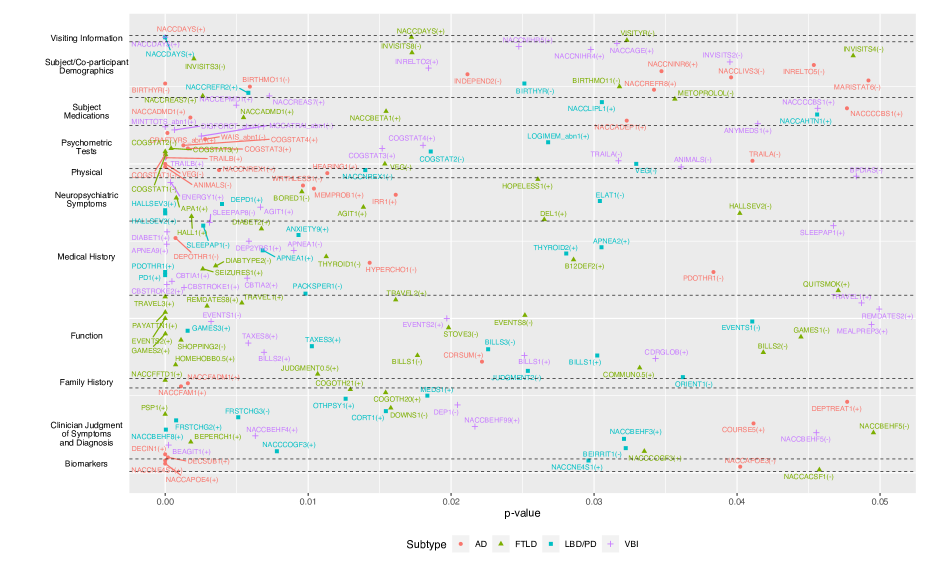
Figure 1: $p$-values of significant predictors (under 5% significance level) associated with the contrast between 4 dementia subtypes and CN, grouped into 11 categories

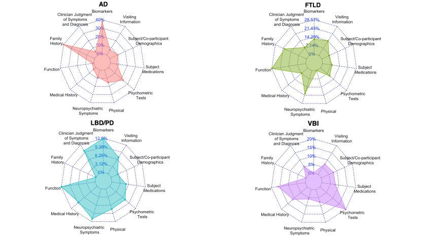
Figure 2: Radar charts of significant predictors (under 5% significance level) in 11 categories for 4 dementia subtypes. Each percentage is the number of significant predictors in a category/total number of predictors in that category, reflecting how many predictors in each category are significant for each subtype.

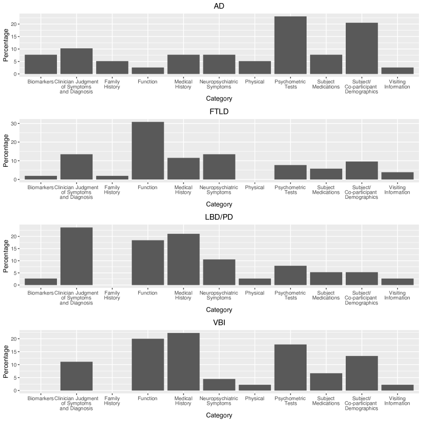
Figure 3: Bar charts of significant predictors (under 5% significance level) in 11 categories for 4 dementia subtypes. Each percentage is the number of significant predictors in a category/total number of significant predictors for the subtype, reflecting the composition of significant predictors for each subtype.

4 Discussions

This paper analyzes the estimation and prediction error of the $\ell_{1}$-penalized multinomial regression model. We also extend the debiased Lasso to the multinomial case to provide valid statistical inference, including the confidence intervals and $p$-values in hypothesis testing. The debiased Lasso is applied to a real dementia data set, where we identify some important variables for the progression into different subtypes of dementia, and the results are highly interpretable. The estimation, inference, and prediction for the contrast-based $\ell_{1}$-penalized multinomial regression model have been implemented in a new R package pemultinom, which is available on CRAN. We believe it will help more practitioners that work with multi-label data.

There are some interesting future research avenues. First, extending the debiasing method and the theory to a more general high-dimensional multi-response setting would be helpful. Second, in this work, we do not consider the sparsity structure between the contrasts associated with different classes. As we mentioned in Section 1.1, Abramovich, Grinshtein and Levy (2021) considers a row-wise sparsity, and we believe it is possible to extend the current analysis to that case. Finally, Dezeure, Bühlmann and Zhang (2017) suggests combining the debiasing method with a residual bootstrap procedure, which is shown to theoretically require weaker conditions and empirically perform better than the debiasing method, especially in simultaneous hypothesis testing problems. It would be interesting if the same idea could be applied to the multinomial regression version of the debiased Lasso.

[Acknowledgments] All the computations were conducted through the High-Performance Computing (HPC) service provided by Columbia University and New York University.

This research was partially supported by NIH Grant P30AG066512, NIH Grant 1R21AG074205-01, a grant from the New York University School of Global Public Health, and the NYU University Research Challenge Fund.

Supplement to “$\ell_{1}$-penalized multinomial regression: Estimation, inference, and prediction, with an application to risk factor identification for different dementia subtypes” We provide the technical proofs of all the theorems in the supplementary material.

References

- Abramovich, Grinshtein and Levy (2021) {barticle}[author] \bauthor\bsnmAbramovich, \bfnmFelix\binitsF., \bauthor\bsnmGrinshtein, \bfnmVadim\binitsV. and \bauthor\bsnmLevy, \bfnmTomer\binitsT. (\byear2021). \btitleMulticlass classification by sparse multinomial logistic regression. \bjournalIEEE Transactions on Information Theory \bvolume67 \bpages4637–4646. \endbibitem
- Ahtiluoto et al. (2010) {barticle}[author] \bauthor\bsnmAhtiluoto, \bfnmS\binitsS., \bauthor\bsnmPolvikoski, \bfnmT\binitsT., \bauthor\bsnmPeltonen, \bfnmM\binitsM., \bauthor\bsnmSolomon, \bfnmA\binitsA., \bauthor\bsnmTuomilehto, \bfnmJaakko\binitsJ., \bauthor\bsnmWinblad, \bfnmB\binitsB., \bauthor\bsnmSulkava, \bfnmR\binitsR. and \bauthor\bsnmKivipelto, \bfnmM\binitsM. (\byear2010). \btitleDiabetes, Alzheimer disease, and vascular dementia: a population-based neuropathologic study. \bjournalNeurology \bvolume75 \bpages1195–1202. \endbibitem
- Battista, Salvatore and Castiglioni (2017) {barticle}[author] \bauthor\bsnmBattista, \bfnmPetronilla\binitsP., \bauthor\bsnmSalvatore, \bfnmChristian\binitsC. and \bauthor\bsnmCastiglioni, \bfnmIsabella\binitsI. (\byear2017). \btitleOptimizing neuropsychological assessments for cognitive, behavioral, and functional impairment classification: a machine learning study. \bjournalBehavioural neurology \bvolume2017. \endbibitem
- Boeve et al. (1998) {barticle}[author] \bauthor\bsnmBoeve, \bfnmBradley F\binitsB. F., \bauthor\bsnmSilber, \bfnmMH\binitsM., \bauthor\bsnmFerman, \bfnmTJ\binitsT., \bauthor\bsnmKokmen, \bfnmE\binitsE., \bauthor\bsnmSmith, \bfnmGE\binitsG., \bauthor\bsnmIvnik, \bfnmRJ\binitsR., \bauthor\bsnmParisi, \bfnmJE\binitsJ., \bauthor\bsnmOlson, \bfnmEJ\binitsE. and \bauthor\bsnmPetersen, \bfnmRC\binitsR. (\byear1998). \btitleREM sleep behavior disorder and degenerative dementia: an association likely reflecting Lewy body disease. \bjournalNeurology \bvolume51 \bpages363–370. \endbibitem
- Chatterjee and Lahiri (2011) {barticle}[author] \bauthor\bsnmChatterjee, \bfnmArindam\binitsA. and \bauthor\bsnmLahiri, \bfnmSoumendra Nath\binitsS. N. (\byear2011). \btitleBootstrapping lasso estimators. \bjournalJournal of the American Statistical Association \bvolume106 \bpages608–625. \endbibitem
- Chatterjee and Lahiri (2013) {barticle}[author] \bauthor\bsnmChatterjee, \bfnmArindam\binitsA. and \bauthor\bsnmLahiri, \bfnmSoumendra N\binitsS. N. (\byear2013). \btitleRates of convergence of the adaptive LASSO estimators to the oracle distribution and higher order refinements by the bootstrap. \bjournalThe Annals of Statistics \bvolume41 \bpages1232–1259. \endbibitem
- Corder et al. (1993) {barticle}[author] \bauthor\bsnmCorder, \bfnmElizabeth H\binitsE. H., \bauthor\bsnmSaunders, \bfnmAnn M\binitsA. M., \bauthor\bsnmStrittmatter, \bfnmWaren J\binitsW. J., \bauthor\bsnmSchmechel, \bfnmDonald E\binitsD. E., \bauthor\bsnmGaskell, \bfnmP Craig\binitsP. C., \bauthor\bsnmSmall, \bfnmGWet\binitsG., \bauthor\bsnmRoses, \bfnmAD\binitsA., \bauthor\bsnmHaines, \bfnmJL\binitsJ. and \bauthor\bsnmPericak-Vance, \bfnmMargaret A\binitsM. A. (\byear1993). \btitleGene dose of apolipoprotein E type 4 allele and the risk of Alzheimer’s disease in late onset families. \bjournalScience \bvolume261 \bpages921–923. \endbibitem
- Dezeure, Bühlmann and Zhang (2017) {barticle}[author] \bauthor\bsnmDezeure, \bfnmRuben\binitsR., \bauthor\bsnmBühlmann, \bfnmPeter\binitsP. and \bauthor\bsnmZhang, \bfnmCun-Hui\binitsC.-H. (\byear2017). \btitleHigh-dimensional simultaneous inference with the bootstrap. \bjournalTest \bvolume26 \bpages685–719. \endbibitem
- Fan and Li (2001) {barticle}[author] \bauthor\bsnmFan, \bfnmJianqing\binitsJ. and \bauthor\bsnmLi, \bfnmRunze\binitsR. (\byear2001). \btitleVariable selection via nonconcave penalized likelihood and its oracle properties. \bjournalJournal of the American Statistical Association \bvolume96 \bpages1348–1360. \endbibitem
- Friedman, Hastie and Tibshirani (2010) {barticle}[author] \bauthor\bsnmFriedman, \bfnmJerome\binitsJ., \bauthor\bsnmHastie, \bfnmTrevor\binitsT. and \bauthor\bsnmTibshirani, \bfnmRob\binitsR. (\byear2010). \btitleRegularization paths for generalized linear models via coordinate descent. \bjournalJournal of statistical software \bvolume33 \bpages1. \endbibitem
- Fu and Knight (2000) {barticle}[author] \bauthor\bsnmFu, \bfnmWenjiang\binitsW. and \bauthor\bsnmKnight, \bfnmKeith\binitsK. (\byear2000). \btitleAsymptotics for lasso-type estimators. \bjournalThe Annals of statistics \bvolume28 \bpages1356–1378. \endbibitem
- Giagkou, Höglinger and Stamelou (2019) {barticle}[author] \bauthor\bsnmGiagkou, \bfnmNikolaos\binitsN., \bauthor\bsnmHöglinger, \bfnmGünter U\binitsG. U. and \bauthor\bsnmStamelou, \bfnmMaria\binitsM. (\byear2019). \btitleProgressive supranuclear palsy. \bjournalInternational review of neurobiology \bvolume149 \bpages49–86. \endbibitem
- Greaves and Rohrer (2019) {barticle}[author] \bauthor\bsnmGreaves, \bfnmCaroline V\binitsC. V. and \bauthor\bsnmRohrer, \bfnmJonathan D\binitsJ. D. (\byear2019). \btitleAn update on genetic frontotemporal dementia. \bjournalJournal of neurology \bvolume266 \bpages2075–2086. \endbibitem
- Hastie et al. (2009) {bbook}[author] \bauthor\bsnmHastie, \bfnmTrevor\binitsT., \bauthor\bsnmTibshirani, \bfnmRobert\binitsR., \bauthor\bsnmFriedman, \bfnmJerome H\binitsJ. H. and \bauthor\bsnmFriedman, \bfnmJerome H\binitsJ. H. (\byear2009). \btitleThe elements of statistical learning: data mining, inference, and prediction \bvolume2. \bpublisherSpringer. \endbibitem
- Hou et al. (2019) {barticle}[author] \bauthor\bsnmHou, \bfnmXiao-He\binitsX.-H., \bauthor\bsnmFeng, \bfnmLei\binitsL., \bauthor\bsnmZhang, \bfnmCan\binitsC., \bauthor\bsnmCao, \bfnmXi-Peng\binitsX.-P., \bauthor\bsnmTan, \bfnmLan\binitsL. and \bauthor\bsnmYu, \bfnmJin-Tai\binitsJ.-T. (\byear2019). \btitleModels for predicting risk of dementia: a systematic review. \bjournalJournal of Neurology, Neurosurgery & Psychiatry \bvolume90 \bpages373–379. \endbibitem
- James et al. (2021) {barticle}[author] \bauthor\bsnmJames, \bfnmCharlotte\binitsC., \bauthor\bsnmRanson, \bfnmJanice M\binitsJ. M., \bauthor\bsnmEverson, \bfnmRichard\binitsR. and \bauthor\bsnmLlewellyn, \bfnmDavid J\binitsD. J. (\byear2021). \btitlePerformance of machine learning algorithms for predicting progression to dementia in memory clinic patients. \bjournalJAMA network open \bvolume4 \bpagese2136553–e2136553. \endbibitem
- Kalaria, Akinyemi and Ihara (2016) {barticle}[author] \bauthor\bsnmKalaria, \bfnmRaj N\binitsR. N., \bauthor\bsnmAkinyemi, \bfnmRufus\binitsR. and \bauthor\bsnmIhara, \bfnmMasafumi\binitsM. (\byear2016). \btitleStroke injury, cognitive impairment and vascular dementia. \bjournalBiochimica et Biophysica Acta (BBA)-Molecular Basis of Disease \bvolume1862 \bpages915–925. \endbibitem
- Lee et al. (2016) {barticle}[author] \bauthor\bsnmLee, \bfnmJason D\binitsJ. D., \bauthor\bsnmSun, \bfnmDennis L\binitsD. L., \bauthor\bsnmSun, \bfnmYuekai\binitsY. and \bauthor\bsnmTaylor, \bfnmJonathan E\binitsJ. E. (\byear2016). \btitleExact post-selection inference, with application to the lasso. \bjournalThe Annals of Statistics \bvolume44 \bpages907–927. \endbibitem
- Licht (2010) {bphdthesis}[author] \bauthor\bsnmLicht, \bfnmChristine\binitsC. (\byear2010). \btitleNew methods for generating significance levels from multiply-imputed data, \btypePhD thesis, \bpublisherOtto-Friedrich-Universität Bamberg, Fakultät Sozial-und Wirtschaftswissenschaften. \endbibitem
- Loh and Wainwright (2015) {barticle}[author] \bauthor\bsnmLoh, \bfnmPo-Ling\binitsP.-L. and \bauthor\bsnmWainwright, \bfnmMartin J\binitsM. J. (\byear2015). \btitleRegularized M-estimators with Nonconvexity: Statistical and Algorithmic Theory for Local Optima. \bjournalJournal of Machine Learning Research \bvolume16 \bpages559–616. \endbibitem
- Loh and Wainwright (2017) {barticle}[author] \bauthor\bsnmLoh, \bfnmPo-Ling\binitsP.-L. and \bauthor\bsnmWainwright, \bfnmMartin J\binitsM. J. (\byear2017). \btitleSupport recovery without incoherence: A case for nonconvex regularization. \bjournalThe Annals of Statistics \bvolume45 \bpages2455–2482. \endbibitem
- Meinshausen and Bühlmann (2006) {barticle}[author] \bauthor\bsnmMeinshausen, \bfnmNicolai\binitsN. and \bauthor\bsnmBühlmann, \bfnmPeter\binitsP. (\byear2006). \btitleHigh-dimensional graphs and variable selection with the lasso. \bjournalThe annals of statistics \bvolume34 \bpages1436–1462. \endbibitem
- Meinshausen, Meier and Bühlmann (2009) {barticle}[author] \bauthor\bsnmMeinshausen, \bfnmNicolai\binitsN., \bauthor\bsnmMeier, \bfnmLukas\binitsL. and \bauthor\bsnmBühlmann, \bfnmPeter\binitsP. (\byear2009). \btitleP-values for high-dimensional regression. \bjournalJournal of the American Statistical Association \bvolume104 \bpages1671–1681. \endbibitem
- Negahban et al. (2012) {barticle}[author] \bauthor\bsnmNegahban, \bfnmSahand N\binitsS. N., \bauthor\bsnmRavikumar, \bfnmPradeep\binitsP., \bauthor\bsnmWainwright, \bfnmMartin J\binitsM. J. and \bauthor\bsnmYu, \bfnmBin\binitsB. (\byear2012). \btitleA unified framework for high-dimensional analysis of -estimators with decomposable regularizers. \bjournalStatistical science \bvolume27 \bpages538–557. \endbibitem
- Onofrj et al. (2013) {barticle}[author] \bauthor\bsnmOnofrj, \bfnmM\binitsM., \bauthor\bsnmTaylor, \bfnmJP\binitsJ., \bauthor\bsnmMonaco, \bfnmD\binitsD., \bauthor\bsnmFranciotti, \bfnmR\binitsR., \bauthor\bsnmAnzellotti, \bfnmF\binitsF., \bauthor\bsnmBonanni, \bfnmL\binitsL., \bauthor\bsnmOnofrj, \bfnmV\binitsV. and \bauthor\bsnmThomas, \bfnmA\binitsA. (\byear2013). \btitleVisual hallucinations in PD and Lewy body dementias: old and new hypotheses. \bjournalBehavioural neurology \bvolume27 \bpages479–493. \endbibitem
- Pencer (2016) {bphdthesis}[author] \bauthor\bsnmPencer, \bfnmMatthew\binitsM. (\byear2016). \btitleFeature Selection and Post-Selection Statistical Inference in Multinomial Models, \btypePhD thesis, \bpublisherMcGill University, Montreal. \endbibitem
- Raskutti, Wainwright and Yu (2011) {barticle}[author] \bauthor\bsnmRaskutti, \bfnmGarvesh\binitsG., \bauthor\bsnmWainwright, \bfnmMartin J\binitsM. J. and \bauthor\bsnmYu, \bfnmBin\binitsB. (\byear2011). \btitleMinimax rates of estimation for high-dimensional linear regression over -balls. \bjournalIEEE transactions on information theory \bvolume57 \bpages6976–6994. \endbibitem
- Reisberg et al. (1982) {barticle}[author] \bauthor\bsnmReisberg, \bfnmBarry\binitsB., \bauthor\bsnmFerris, \bfnmSteven H\binitsS. H., \bauthor\bparticlede \bsnmLeon, \bfnmMony J\binitsM. J. and \bauthor\bsnmCrook, \bfnmThomas\binitsT. (\byear1982). \btitleThe Global Deterioration Scale for assessment of primary degenerative dementia. \bjournalThe American journal of psychiatry. \endbibitem
- Reisberg et al. (2010) {barticle}[author] \bauthor\bsnmReisberg, \bfnmBarry\binitsB., \bauthor\bsnmShulman, \bfnmMelanie B\binitsM. B., \bauthor\bsnmTorossian, \bfnmCarol\binitsC., \bauthor\bsnmLeng, \bfnmLing\binitsL. and \bauthor\bsnmZhu, \bfnmWei\binitsW. (\byear2010). \btitleOutcome over seven years of healthy adults with and without subjective cognitive impairment. \bjournalAlzheimer’s & Dementia \bvolume6 \bpages11–24. \endbibitem
- Rubin (2004) {bbook}[author] \bauthor\bsnmRubin, \bfnmDonald B\binitsD. B. (\byear2004). \btitleMultiple imputation for nonresponse in surveys \bvolume81. \bpublisherJohn Wiley & Sons. \endbibitem
- Sartori (2011) {barticle}[author] \bauthor\bsnmSartori, \bfnmSamantha\binitsS. (\byear2011). \btitlePenalized regression: Bootstrap confidence intervals and variable selection for high-dimensional data sets. \endbibitem
- Solntsev, Nocedal and Byrd (2015) {barticle}[author] \bauthor\bsnmSolntsev, \bfnmStefan\binitsS., \bauthor\bsnmNocedal, \bfnmJorge\binitsJ. and \bauthor\bsnmByrd, \bfnmRichard H\binitsR. H. (\byear2015). \btitleAn algorithm for quadratic -regularized optimization with a flexible active-set strategy. \bjournalOptimization Methods and Software \bvolume30 \bpages1213–1237. \endbibitem
- Taylor and Tibshirani (2015) {barticle}[author] \bauthor\bsnmTaylor, \bfnmJonathan\binitsJ. and \bauthor\bsnmTibshirani, \bfnmRobert J\binitsR. J. (\byear2015). \btitleStatistical learning and selective inference. \bjournalProceedings of the National Academy of Sciences \bvolume112 \bpages7629–7634. \endbibitem
- R Core Team (2020) {bmanual}[author] \bauthor\bsnmR Core Team (\byear2020). \btitleR: A Language and Environment for Statistical Computing \bpublisherR Foundation for Statistical Computing, \baddressVienna, Austria. \endbibitem
- Thabtah, Ong and Peebles (2022) {barticle}[author] \bauthor\bsnmThabtah, \bfnmFadi\binitsF., \bauthor\bsnmOng, \bfnmSwan\binitsS. and \bauthor\bsnmPeebles, \bfnmDavid\binitsD. (\byear2022). \btitleDetection of Dementia Progression from Functional Activities Data using Machine Learning Techniques. \bjournalIntelligent Decision Technologies \bvolume16 \bpages615–630. \endbibitem
- Tian et al. (2023a) {barticle}[author] \bauthor\bsnmTian, \bfnmYe\binitsY., \bauthor\bsnmRusinek, \bfnmHenry\binitsH., \bauthor\bsnmV. Masurkar, \bfnmArjun\binitsA. and \bauthor\bsnmFeng, \bfnmYang\binitsY. (\byear2023a). \btitleRisk factor to predict dementia subtypes: an analysis of the NACC database. \bjournalsubmitted. \endbibitem
- Tian et al. (2023b) {barticle}[author] \bauthor\bsnmTian, \bfnmYe\binitsY., \bauthor\bsnmRusinek, \bfnmHenry\binitsH., \bauthor\bsnmV. Masurkar, \bfnmArjun\binitsA. and \bauthor\bsnmFeng, \bfnmYang\binitsY. (\byear2023b). \btitleSupplement to “-penalized multinomial regression: Estimation, inference, and prediction, with an application to risk factor identification for different dementia subtypes”. \endbibitem
- Tibshirani (1996) {barticle}[author] \bauthor\bsnmTibshirani, \bfnmRobert\binitsR. (\byear1996). \btitleRegression shrinkage and selection via the lasso. \bjournalJournal of the Royal Statistical Society: Series B (Methodological) \bvolume58 \bpages267–288. \endbibitem
- Van de Geer et al. (2014) {barticle}[author] \bauthor\bparticleVan de \bsnmGeer, \bfnmSara\binitsS., \bauthor\bsnmBühlmann, \bfnmPeter\binitsP., \bauthor\bsnmRitov, \bfnmYa’acov\binitsY. and \bauthor\bsnmDezeure, \bfnmRuben\binitsR. (\byear2014). \btitleOn asymptotically optimal confidence regions and tests for high-dimensional models. \bjournalThe Annals of Statistics \bvolume42 \bpages1166–1202. \endbibitem
- Wasserman and Roeder (2009) {barticle}[author] \bauthor\bsnmWasserman, \bfnmLarry\binitsL. and \bauthor\bsnmRoeder, \bfnmKathryn\binitsK. (\byear2009). \btitleHigh dimensional variable selection. \bjournalAnnals of statistics \bvolume37 \bpages2178. \endbibitem
- Yuan and Lin (2006) {barticle}[author] \bauthor\bsnmYuan, \bfnmMing\binitsM. and \bauthor\bsnmLin, \bfnmYi\binitsY. (\byear2006). \btitleModel selection and estimation in regression with grouped variables. \bjournalJournal of the Royal Statistical Society: Series B (Statistical Methodology) \bvolume68 \bpages49–67. \endbibitem
- Zhang (2010) {barticle}[author] \bauthor\bsnmZhang, \bfnmCun-Hui\binitsC.-H. (\byear2010). \btitleNearly unbiased variable selection under minimax concave penalty. \bjournalThe Annals of Statistics \bvolume38 \bpages894–942. \endbibitem
- Zhang, Khalili and Asgharian (2022) {barticle}[author] \bauthor\bsnmZhang, \bfnmDongliang\binitsD., \bauthor\bsnmKhalili, \bfnmAbbas\binitsA. and \bauthor\bsnmAsgharian, \bfnmMasoud\binitsM. (\byear2022). \btitlePost-model-selection inference in linear regression models: An integrated review. \bjournalStatistics Surveys \bvolume16 \bpages86–136. \endbibitem
- Zhang and Zhang (2014) {barticle}[author] \bauthor\bsnmZhang, \bfnmCun-Hui\binitsC.-H. and \bauthor\bsnmZhang, \bfnmStephanie S\binitsS. S. (\byear2014). \btitleConfidence intervals for low dimensional parameters in high dimensional linear models. \bjournalJournal of the Royal Statistical Society: Series B (Statistical Methodology) \bvolume76 \bpages217–242. \endbibitem
- Zhao and Yu (2006) {barticle}[author] \bauthor\bsnmZhao, \bfnmPeng\binitsP. and \bauthor\bsnmYu, \bfnmBin\binitsB. (\byear2006). \btitleOn model selection consistency of Lasso. \bjournalThe Journal of Machine Learning Research \bvolume7 \bpages2541–2563. \endbibitem
- Zou (2006) {barticle}[author] \bauthor\bsnmZou, \bfnmHui\binitsH. (\byear2006). \btitleThe adaptive lasso and its oracle properties. \bjournalJournal of the American statistical association \bvolume101 \bpages1418–1429. \endbibitem
- Zou and Hastie (2005) {barticle}[author] \bauthor\bsnmZou, \bfnmHui\binitsH. and \bauthor\bsnmHastie, \bfnmTrevor\binitsT. (\byear2005). \btitleRegularization and variable selection via the elastic net. \bjournalJournal of the royal statistical society: series B (statistical methodology) \bvolume67 \bpages301–320. \endbibitem