Efficient Adaptive Joint Significance Tests and Sobel-Type Confidence Intervals for Mediation Effects

Abstract

Mediation analysis is an important statistical tool in many research fields. Its aim is to investigate the mechanism along the causal pathway between an exposure and an outcome. The joint significance test is widely utilized as a prominent statistical approach for examining mediation effects in practical applications. Nevertheless, the limitation of this mediation testing method stems from its conservative Type I error, which reduces its statistical power and imposes certain constraints on its popularity and utility. The joint significance tests for large-scale mediation hypotheses in genome-wide epigenetic research have been extensively investigated, whereas these methods are not applicable to single or small-scale mediation hypotheses. The proposed solution to address this gap is the adaptive joint significance test for one mediator, a novel data-adaptive test for mediation effect that exhibits significant advancements compared to traditional joint significance test. The proposed method is designed to be user-friendly, eliminating the need for complicated procedures. We have derived explicit expressions for size and power, ensuring the theoretical validity of our approach. Furthermore, we extend the proposed adaptive joint significance tests for small-scale mediation hypotheses with family-wise error rate (FWER) control. Additionally, a novel adaptive Sobel-type approach is proposed for the estimation of confidence intervals for the mediation effects, demonstrating significant advancements over conventional Sobel’s confidence intervals in terms of achieving desirable coverage probabilities. Our mediation testing and confidence intervals procedure is evaluated through comprehensive simulations, and compared with numerous existing approaches. Finally, we illustrate the usefulness of our method by analysing three real-world datasets with continuous, binary and time-to-event outcomes, respectively.

Keywords: Confidence intervals; Joint significance test; Adaptive Sobel’s test; Multiple mediators; Small-scale mediation hypotheses.

1 Introduction

Mediation analysis plays an important role in understanding the causal mechanism that an independent variable $X$ affects a dependent variable $Y$ through an intermediate variable (mediator) $M$. The application of mediation analysis is widely popular in many fields, such as psychology, economics, epidemiology, medicine, sociology, behavioral science, and many others. From the view point of methodological development, Baron and Kenny (1986) has laid a foundation for the development of mediation analysis. Afterwards, there have been a great deal of papers on this topic. Just to name a few: Mackinnon et al. (2004) constructed the confidence limits for indirect effect by resampling methods. Wang and Zhang (2011) and Zhang and Wang (2013) introduced the estimating and testing methods for mediation effects with censored data and missing data, respectively. Shen et al. (2014) proposed an inference technique for quantile mediation effects. Zhang et al. (2016) introduced a joint significance test method for high-dimensional mediation effects by sure independent screening and minimax concave penalty techniques. VanderWeele and Tchetgen (2017) considered causal mediation analysis with time-varying exposures and mediators. Sun et al. (2021) proposed a Bayesian modeling approach for mediation analysis. Zhou (2022) introduced a semiparametric estimation method for mediation analysis with multiple causally ordered mediators. For more results about mediation analysis, we refer to three reviewing papers by MacKinnon et al. (2007), Preacher (2015) and Zhang et al. (2022).

In the area of mediation analysis, the joint significance test is an important statistical method for investigating the causal mechanism of mediation effects MacKinnon (2008). However, the main shortcoming of this method is due to the conservative type I error of mediation testing MacKinnon et al. (2002), which largely prevents its popularity for practical users. The estimation of confidence interval for the mediation effect is a crucial aspect in mediation analysis, where the Sobel-type (or normality-based) method is consistently employed to construct these intervals. The performance of Sobel-type confidence interval, however, falls short when the mediation effect is zero. To improve the performances of joint significance test and Sobel-type confidence interval, we propose two novel data-adaptive statistical mediation analysis methods with theoretical verification. The main advantages of our proposed method are as follows: First, the adaptive joint significance test and adaptive sobel-type confidence interval are two flexible and data-driven methods. Particularly, it is very convenient to implement the two proposed methods from the view of practical application. i.e., our method is user-friendly without involving complicated procedures. Second, compared to the conventional joint significance test, our test method has significantly improved in terms of size and power. The enhanced powers are especially obvious for those relatively weak mediation effects, which are difficult to be recognized as significant mediators by traditional methods. Third, the explicit formulation of the coverage probability for the adaptive Sobel-type confidence interval is provided to ensure the validity of our procedure.

The remainder of this paper is organized as follows: In Section 2, we review some details about the traditional joint significance test for mediation effects. Then we propose a novel data-adaptive joint significance test for one mediator, together with the explicit expressions of size and power. Meanwhile, an adaptive Sobel test is also introduced, which shows a significant improvement compared to traditional Sobel’s method. In Section 3, we implement the adaptive joint significance test towards small-scale multiple testing with FWER control. Section 4 introduces a data-driven approach to construct a confidence interval for the mediation effect. Section 5 presents some simulation studies to assess the performance of our method. In Section 6, we perform mediation analysis for three real-world datasets with our proposed method. Some concluding remarks are provided in Section 7. All proof details of theorems are presented in the Supplementary Materials.

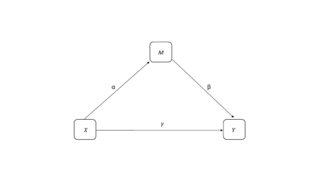
Figure 1: A scenario of mediation model with one mediator (confounding variables are omitted).

2 Adaptive Joint Significance Test

To begin with, we review some basic notations in the framework of mediation analysis. Let $X$ be an exposure, $M$ be the mediator and $Y$ be the outcome (see Figure 1). As described by MacKinnon (2008), the aim of mediation analysis is focused on investigating the causal mechanism along the pathway $X\rightarrow M\rightarrow Y$. Generally speaking, the causal effect $X\rightarrow M$ is parameterized by $\alpha$ (after adjusting for confounders), and the causal effect $M\rightarrow Y$ is parameterized by $\beta$ (after adjusting for exposure and confounders). In this case, the mediating effect of $M$ is described by $\alpha\beta$, which is commonly referred to as the “product-coefficient” approach MacKinnon et al. (2002). To evaluate whether $M$ plays an intermediary role between $X$ and $Y$, it is customary to conduct hypothesis testing at a significance level of $\delta$ as follows:

$$H_{0}:~{}\alpha\beta=0~{}\leftrightarrow~{}H_{A}:\alpha\beta\neq 0.$$ (1)

If the null hypothesis is rejected, we could regard $M$ as a significant mediator along the pathway $X\rightarrow M\rightarrow Y$. It is worth to pointing out that the null hypothesis $H_{0}$ is composite. To be specific, $H_{0}$ can be equivalently decomposed into the union of three disjoint component null hypotheses $H_{0}=H_{00}\cup H_{01}\cup H_{10}$, where

$$H_{00}:~{}\alpha=0,\beta=0;$$

$$H_{01}:~{}\alpha=0,\beta\neq 0;$$

$$H_{10}:~{}\alpha\neq 0,\beta=0.$$

Let $T_{\alpha}$ and $T_{\beta}$ be the statistics for testing $\alpha=0$ and $\beta=0$, respectively. Under the null hypothesis, as the sample size tends towards infinity, it can be observed that

$$T_{\alpha}=\frac{\hat{\alpha}}{\hat{\sigma}_{\alpha}}\sim N(0,1)~{}{\rm and}~{}T_{\beta}=\frac{\hat{\beta}}{\hat{\sigma}_{\beta}}\sim N(0,1),$$ (2)

where $\hat{\alpha}$ and $\hat{\beta}$ are the estimates for $\alpha$ and $\beta$, respectively. $\hat{\sigma}_{\alpha}$ and $\hat{\sigma}_{\beta}$ are the estimated standard errors of $\hat{\alpha}$ and $\hat{\beta}$, respectively. The corresponding p-values for $T_{\alpha}$ and $T_{\beta}$ are

$$P_{\alpha} = 2\{1-\Phi_{N(0,1)}(|T_{\alpha}|)\},$$ (3)

$$P_{\beta} = 2\{1-\Phi_{N(0,1)}(|T_{\beta}|)\},$$ (4)

where $T_{\alpha}$ and $T_{\beta}$ are defined in (2). In the field of mediation analysis, one of the most popular method for (1) is the joint significance (JS) test (also known as the MaxP test). The idea of JS test is that we can reject $H_{0}$ if both $\alpha=0$ and $\beta=0$ are simultaneously rejected. i.e., the JS test statistic is defined as

$$P_{JS}=\max(P_{\alpha},P_{\beta}),$$ (5)

where $P_{\alpha}$ and $P_{\beta}$ are given in (3) and (4), respectively. Due to the convenience of JS test in practical application, it has been widely adopted by many research fields, such as the social and biomedical sciences. However, the JS test suffers from overly conservative type I error, especially when both $\alpha=0$ and $\beta=0$ MacKinnon et al. (2002). In fact, this is a long-existed and unresolved problem for the Sobel test. To bridge this gap, we propose a novel data-adaptive method for improving the statistical efficiency of the Sobel test, especially focusing on the conservative issue in the case of $\alpha=\beta=0$.

Under $H_{0}$, the traditional JS test regards $P_{JS}$ as a uniform random variable over $(0,1)$. i.e., $P_{JS}\sim U(0,1)$. However, the actual distribution of $P_{JS}$ is not $U(0,1)$ under the component null hypotheses $H_{00}$, which is the reason of the conservative performance of traditional JS test. To provide more insights on this issue, suppose that $Z_{1}$ and $Z_{2}$ are two independent random variables following U(0,1) distribution. Let ${Z}=\max({Z_{1}},{Z_{2}})$ and its density function is denoted as $f_{{Z}}(z)$. The distribution function of $Z$ is

$$F_{Z}(z)=\mathbb{P}(Z\leq z)=\mathbb{P}(Z_{1}\leq z,Z_{2}\leq z)=\mathbb{P}(Z_{1}\leq z)\mathbb{P}(Z_{2}\leq z)=z^{2},$$

i.e., the density function of $Z$ is $f_{Z}(z)=\frac{1}{2}z$ for $0\leq z\leq 1$ and $f_{Z}(z)=0$, otherwise. Therefore, the maximum of two independent p-values ($P_{JS}$) does not follow $U(0,1)$. This provides a theoretical view about the conservative performance of JS test when both $\alpha=0$ and $\beta=0$. Note that the distribution function of $Z^{2}=\{\max({Z_{1}},{Z_{2}})\}^{2}$ is

$$F_{Z^{2}}(z) = \mathbb{P}(Z^{2}\leq z)$$ (9)

$$= \mathbb{P}(Z_{1}\leq z^{1/2})\mathbb{P}(Z_{2}\leq z^{1/2})$$

$$= \left\{\begin{array}[]{ll}0,&z<0,\\ z,&0\leq z<1,\\ 1,&z\geq 1.\end{array}\right.$$

i.e., under $H_{00}$ the squared maximum of two p-values ($P^{2}_{JS}$) has an uniform distribution over (0, 1). This finding sheds light on the solution to the conservative issue of conventional JS test.

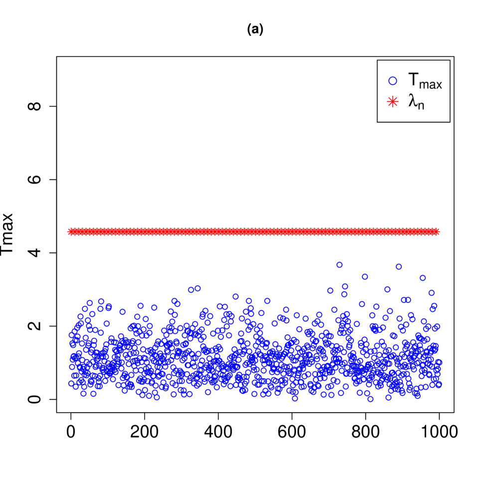
(a) The parameter is $(\alpha,\beta)=(0,0)$.

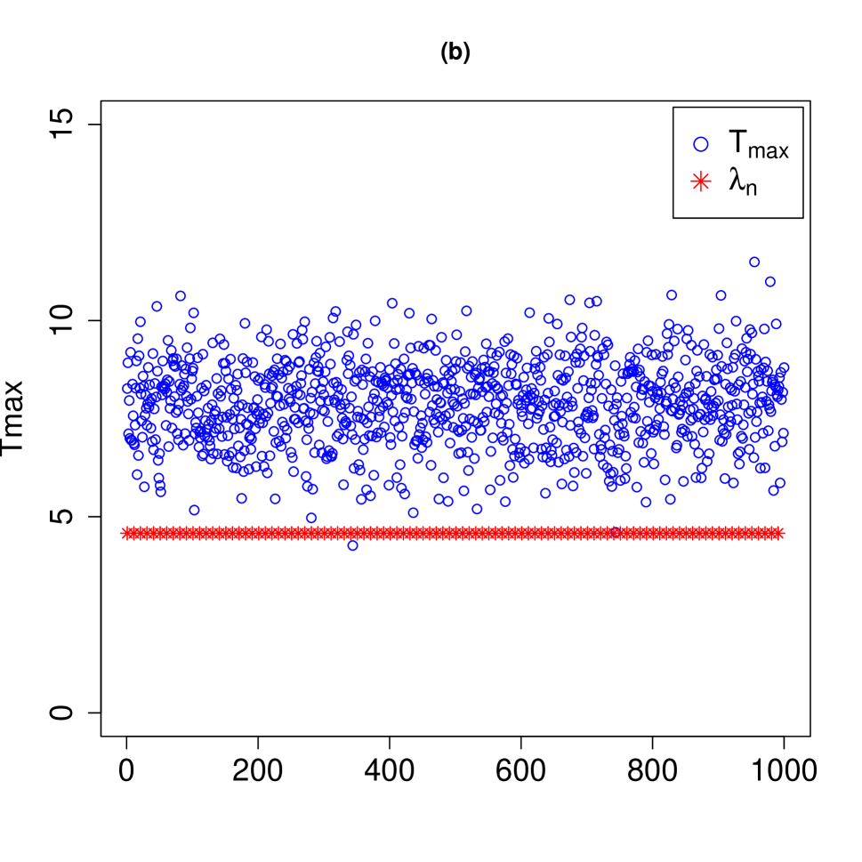
(b) The parameter is $(\alpha,\beta)=(0.25,0)$.

Figure 2: The scatter plots of $T_{max}=\max\{|T_{\alpha}|,|T_{\beta}|\}$ and $\lambda_{n}=\sqrt{n}/\log(n)$ with 1000 repetitions.

To deal with this problem, we try to reasonably distinguish $H_{00}$ from $H_{01}$ and $H_{10}$ using a certain criterion. Under $H_{00}$, we have $\lim_{n\rightarrow\infty}\mathbb{P}(|T_{\alpha}|<\lambda_{n},|T_{\beta}|<\lambda_{n}|H_{00})=1$, where $\lambda_{n}=o(\sqrt{n})$ and $\lambda_{n}\rightarrow\infty$ as $n\rightarrow\infty$. However, $\lim_{n\rightarrow\infty}\mathbb{P}(|T_{\alpha}|<\lambda_{n},|T_{\beta}|<\lambda_{n}|H_{10})=0$ and $\lim_{n\rightarrow\infty}\mathbb{P}(|T_{\alpha}|<\lambda_{n},|T_{\beta}|<\lambda_{n}|H_{01})=0$. In view of these points, we are likely to regard the null hypothesis $H_{0}$ as $H_{00}$ instead of $H_{01}$ or $H_{10}$ when $\max\{|T_{\alpha}|,|T_{\beta}|\}<\lambda_{n}$. This point is the key idea that stimulates the development of our method. We provide a numerical example to illustrate the above-mentioned spirit. Specifically, we generate a series of random samples from the linear mediation models: $Y=0.5+0.5X+\beta M+\epsilon$ and $M=0.5+\alpha X+e$, where $X$, $\epsilon$ and $e$ follow from $N(0,1)$. The resulting $T_{\alpha}$ and $T_{\beta}$ are obtained by the ordinary least square method. In Figure 2, we present the scatter plots of $T_{max}=\max\{|T_{\alpha}|,|T_{\beta}|\}$ and $\lambda_{n}=\sqrt{n}/\log(n)$ with 1000 repetitions, where the sample size is $n=1000$, the parameters $(\alpha,\beta)$ are chosen as $(\alpha,\beta)=(0,0)$, and (0.25, 0), respectively. The observation from Figure 2 suggests that, under the assumption of $\alpha=\beta=0$, there is a high probability that $T_{max}$ is significantly smaller than $\lambda_{n}$ as $n\rightarrow\infty$. However, $T_{max}$ is asymptotically much larger than $\lambda_{n}$ when $\alpha\neq 0$, and the same conclusion also applies to $\beta\neq 0$.

Motivated by the above findings, we propose a novel adaptive joint significance (AJS) test procedure for (1), where the p-value is defined as

$$P_{AJS} = \left\{\begin{array}[]{ll}P_{JS},&\max\{|T_{\alpha}|,|T_{\beta}|\}\geq\lambda_{n},\\ P^{2}_{JS},&\max\{|T_{\alpha}|,|T_{\beta}|\}<\lambda_{n}.\end{array}\right.$$ (12)

Here, the threshold is chosen as $\lambda_{n}=\sqrt{n}/\log(n)$ satisfying $\lambda_{n}=o(\sqrt{n})$ and $\lambda_{n}\rightarrow\infty$ as $n\rightarrow\infty$; $T_{\alpha}$, $T_{\beta}$ and $P_{JS}$ are given in (2) and (5), respectively. In Figure 3, we provide an illustrative example of the p-values for AJS and JS methods with $(\alpha,\beta)=(0,0)$ and $n=2000$. The data are generated from the same models of Figure 2 with 5000 repetitions. The distribution of $P_{AJS}$ is observed to be uniform in Figure 3, whereas the histogram indicates a right skewness in the distribution of $P_{JS}$. Moreover, the Figure 3 provides an intuitive explanation for the conservatism of traditional JS method when $\alpha=\beta=0$.

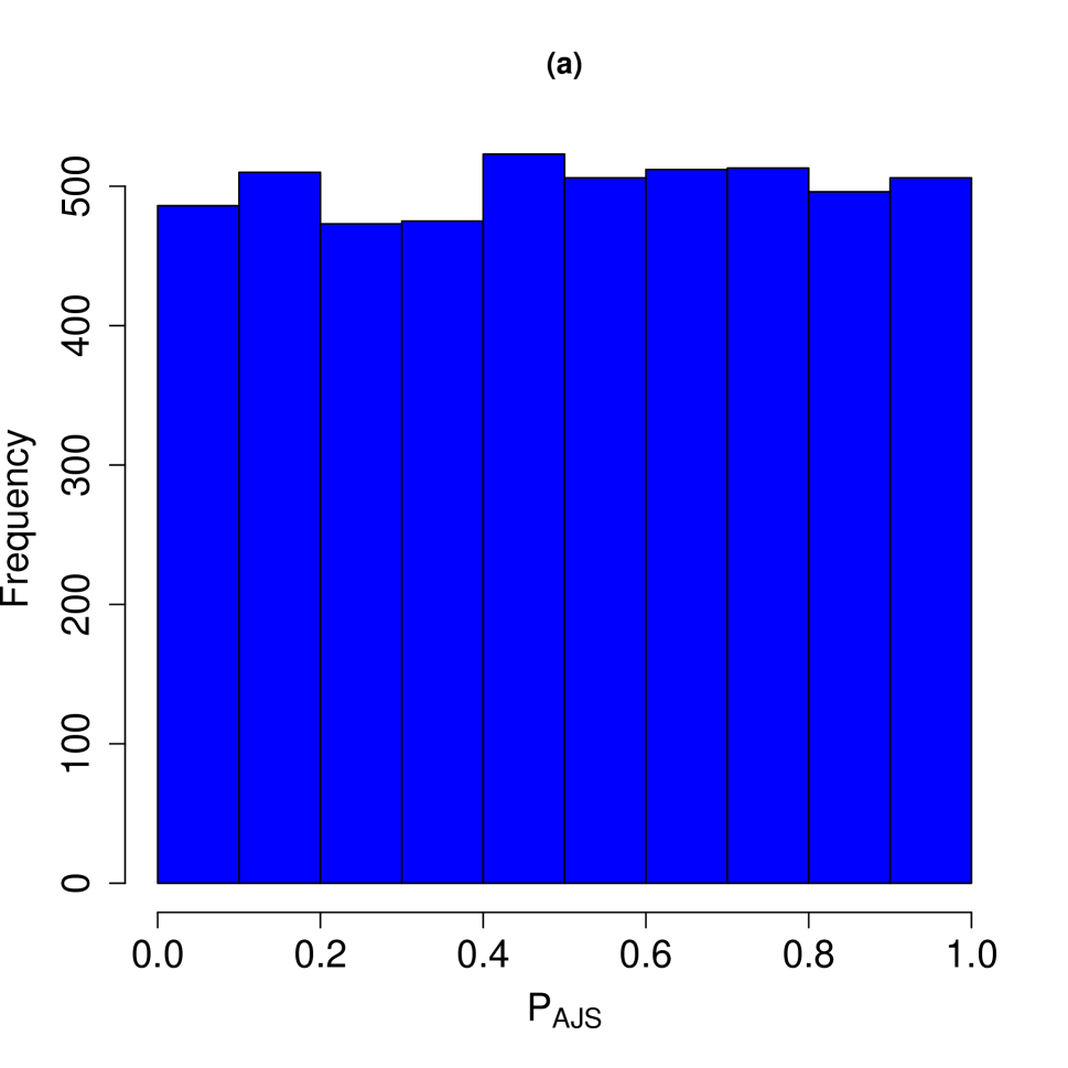
(a) The p-values of AJS method.

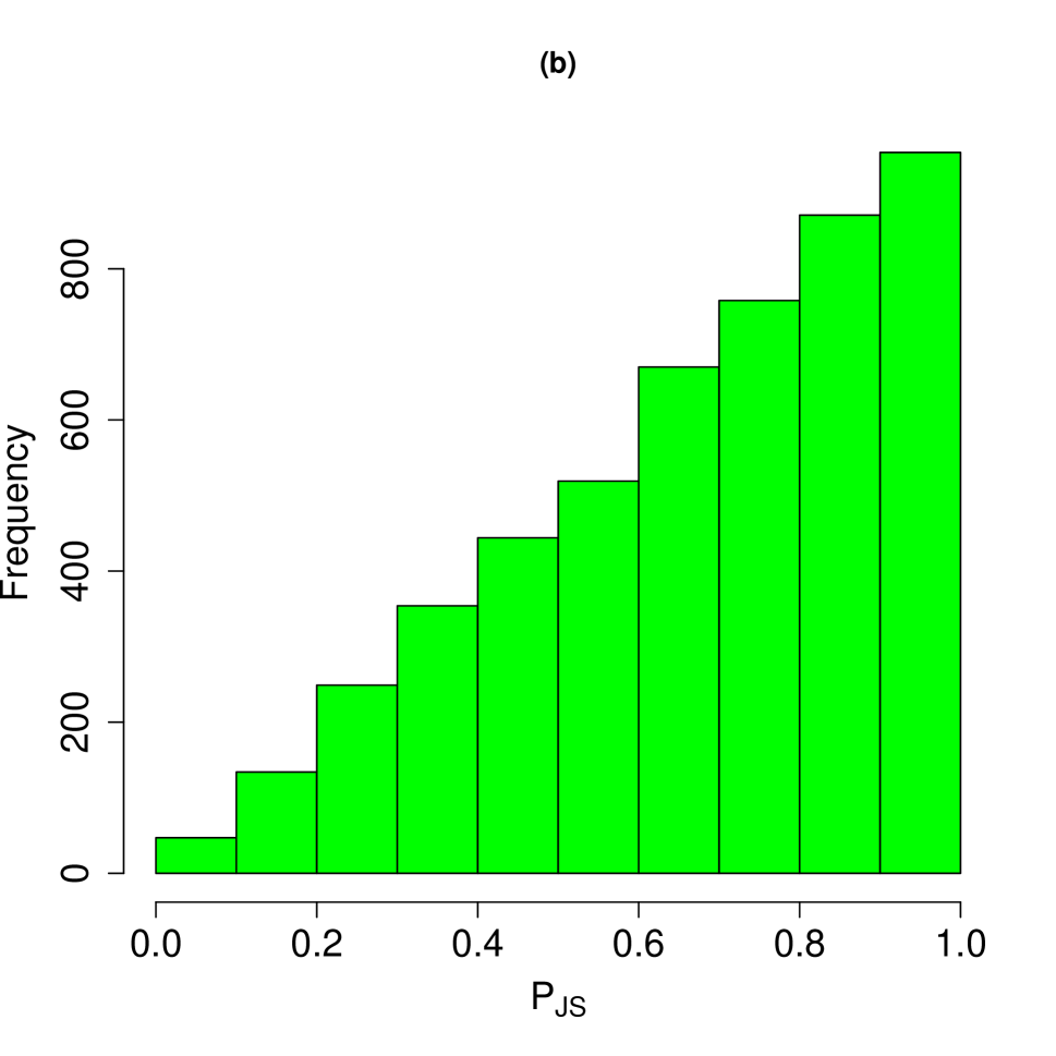
(b) The p-values of JS method.

Figure 3: The histogram of p-values for $(\alpha,\beta)=(0,0)$ with $\lambda_{n}=\sqrt{n}/\log(n)$.

The decision rule of AJS test is that the null hypothesis $H_{0}$ is rejected if $P_{AJS}$ is much smaller than the significance level $\delta$. i.e., we can regard $M$ as a significant mediator when $P_{AJS}<\delta$ in practical application, where $P_{AJS}$ is defined by (12). Furthermore, we derive the explicit expressions of size and power in Theorem 1, which is useful for ensuring rationality of the AJS test.

Theorem 1

Given that $\lambda_{n}=o(\sqrt{n})$ and as the sample size $n$ approaches infinity, under $H_{00}$ the asymptotic size of our proposed AJS test for (1) is

$$\lim\limits_{n\rightarrow\infty}{Size(AJS|H_{00})}=\delta,$$ (13)

where $\delta$ is the significance level. Under $H_{10}$, with probability approaching one, the asymptotic size of the AJS test is

$$\lim\limits_{n\rightarrow\infty}{Size(AJS|H_{10})} = \delta.$$ (14)

Similarly, with probability approaching one, under $H_{01}$ the asymptotic size of the AJS test is

$$\lim_{n\rightarrow\infty}{Size(AJS|H_{01})}=\delta.$$

Moreover, the power of the AJS test can be written as

$$Power(AJS) = \mathbb{P}\big{(}T_{max}\geq\lambda_{n}|H_{A}\big{)}Power\big{(}AJS|T_{max}\geq\lambda_{n}\big{)}$$

$$~{}+\mathbb{P}\big{(}T_{max}<\lambda_{n}|H_{A}\big{)}Power\big{(}AJS|T_{max}<\lambda_{n}\big{)},$$

where $T_{max}=\max\{|T_{\alpha}|,|T_{\beta}|\}$, together with

$$Power\big{(}AJS|T_{max}\geq\lambda_{n}\big{)} = \Big{[}\Phi_{N(0,1)}\big{(}\mu_{\alpha}-N_{1-\delta/2}(0,1)\big{)}+\Phi_{N(0,1)}\big{(}-\mu_{\alpha}-N_{1-\delta/2}(0,1)\big{)}\Big{]}$$

$$\times\Big{[}\Phi_{N(0,1)}\big{(}\mu_{\beta}-N_{1-\delta/2}(0,1)\big{)}+\Phi_{N(0,1)}\big{(}-\mu_{\beta}-N_{1-\delta/2}(0,1)\big{)}\Big{]}$$

and

$$Power\big{(}AJS|T_{max}<\lambda_{n}\big{)} = \Big{[}\Phi_{N(0,1)}\big{(}\mu_{\alpha}-N_{1-\sqrt{\delta}/2}(0,1)\big{)}+\Phi_{N(0,1)}\big{(}-\mu_{\alpha}-N_{1-\sqrt{\delta}/2}(0,1)\big{)}\Big{]}$$

$$\times\Big{[}\Phi_{N(0,1)}\big{(}\mu_{\beta}-N_{1-\sqrt{\delta}/2}(0,1)\big{)}+\Phi_{N(0,1)}\big{(}-\mu_{\beta}-N_{1-\sqrt{\delta}/2}(0,1)\big{)}\Big{]},$$

where $\mu_{\alpha}=\mathbb{E}(\hat{\alpha}/\hat{\sigma}_{\alpha})$ and $\mu_{\beta}=\mathbb{E}(\hat{\beta}/\hat{\sigma}_{\beta})$.

Theoretically, we compare the AJS with traditional JS in terms of size and power. First, under $H_{00}$ the size of traditional JS test for (1) is

$$Size(JS|H_{00}) = \mathbb{P}(P_{JS}<\delta|H_{00})$$

$$= \mathbb{P}(P_{\alpha}<\delta|H_{00})\mathbb{P}(P_{\beta}<\delta|H_{00})$$

$$= \delta^{2},$$

which explains the conservative phenomenon of traditional JS test. Based on (13), $Size(AJS|H_{00})$ is much larger than $Size(JS|H_{00})$ as $n\rightarrow\infty$. Second, the power of traditional JS test for (1) was given by Liu et al. (2022):

$$Power\big{(}JS) = \Big{[}\Phi_{N(0,1)}\big{(}\mu_{\alpha}-N_{1-\delta/2}(0,1)\big{)}+\Phi_{N(0,1)}\big{(}-\mu_{\alpha}-N_{1-\delta/2}(0,1)\big{)}\Big{]}$$

$$\times\Big{[}\Phi_{N(0,1)}\big{(}\mu_{\beta}-N_{1-\delta/2}(0,1)\big{)}+\Phi_{N(0,1)}\big{(}-\mu_{\beta}-N_{1-\delta/2}(0,1)\big{)}\Big{]}.$$

From (1) and (2), we can derive that

$$Power\big{(}AJS)-Power\big{(}JS)=$$

$$\mathbb{P}\big{(}T_{max}<\lambda_{n}|H_{A}\big{)}\Big{[}Power\big{(}AJS|T_{max}<\lambda_{n}\big{)}-Power\big{(}AJS|T_{max}\geq\lambda_{n}\big{)}\Big{]}.$$

In view of the fact that $N_{1-\sqrt{\delta}/2}(0,1)<N_{1-{\delta}/2}(0,1)$, so $Power\big{(}AJS)$ is much larger than $Power\big{(}JS)$, especially for those mediators with relatively weak mediation effects. However, $Power\big{(}AJS)$ is close to $Power\big{(}JS)$ if both $\alpha$ and $\beta$ are large. The reason is due to $\mathbb{P}\big{(}T_{max}<\lambda_{n}|H_{A}\big{)}\approx 0$ in this situation. As a whole, the proposed AJS method is obviously better than the conventional JS test in many situations. Simulations will be used to support this conclusion.

In the field of mediation analysis, another popular method for (1) is the Sobel test Sobel (1982), and the corresponding test statistic is

$$T_{Sobel}=\frac{\hat{\alpha}\hat{\beta}}{\{\hat{\alpha}^{2}\hat{\sigma}^{2}_{\beta}+\hat{\beta}^{2}\hat{\sigma}^{2}_{\alpha}\}^{1/2}},$$ (17)

where $\hat{\alpha}$ and $\hat{\beta}$ are the estimates for $\alpha$ and $\beta$, respectively. $\hat{\sigma}_{\alpha}$ and $\hat{\sigma}_{\beta}$ are the estimated standard errors of $\hat{\alpha}$ and $\hat{\beta}$, respectively. The decision rule of traditional Sobel test relies on the standard asymptotic normality of $T_{Sobel}$. i.e., we can reject $H_{0}$ if the $p$-value, $P_{Sobel}$, is smaller than a specified significance level $\delta$, where

$$P_{Sobel}=2\{1-\Phi_{N(0,1)}(|T_{Sobel}|)\},$$

and $\Phi_{N(0,1)}(\cdot)$ is the cumulative distribution function of $N(0,1)$. Due to the convenience of Sobel test in practical application, it has been widely adopted by many research fields, such as the social and biomedical sciences. However, the Sobel test suffers from overly conservative type I error, especially when both $\alpha=0$ and $\beta=0$ MacKinnon et al. (2002). From Liu et al. (2022), the Sobel statistic $T_{sobel}$ has an asymptotic normal distribution $N(0,1)$ under $H_{01}$ and $H_{10}$, while its asymptotic distribution is $N(0,1/4)$ in the case of $H_{00}$. Therefore, the performance of traditional Sobel test is conservative when $\alpha=0$ and $\beta=0$. In fact, this is a long-existed and unresolved problem for the Sobel test. Similar to the idea of AJS method, we propose a novel adaptive Sobel (ASobel) test procedure for (1), and the p-value is defined as

$$P_{ASobel} = \left\{\begin{array}[]{ll}2\{1-\Phi_{N(0,1)}(|T_{Sobel}|)\},&\max\{|T_{\alpha}|,|T_{\beta}|\}\geq\lambda_{n},\\ 2\{1-\Phi_{N(0,1/4)}(|T_{Sobel}|)\},&\max\{|T_{\alpha}|,|T_{\beta}|\}<\lambda_{n},\end{array}\right.$$ (20)

where $\Phi_{N(0,1/4)}(\cdot)$ is the cumulative distribution function of $N(0,1/4)$; $T_{\alpha}$, $T_{\beta}$ and $\lambda_{n}$ are the same as that of $P_{AJS}$ in (12). The decision rule of the ASobel test states that the null hypothesis $H_{0}$ is rejected if the test statistic ($P_{ASobel}$) is significantly smaller than the predetermined significance level $\delta$. The p-values for ASobel and Sobel methods with $(\alpha,\beta)=(0,0)$ and $n=2000$ are illustrated in Figure 4. The sample data are the same as depicted in Figure 4. The distribution of $P_{ASobel}$ appears to be uniformly distributed in Figure 4, while the histogram indicates a right-skewed distribution for $P_{Sobel}$. The Figure 4 further elucidates the inherent conservatism of the traditional Sobel method when both $\alpha$ and $\beta$ are set to zero.

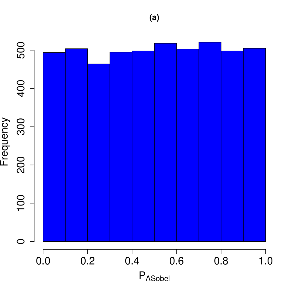
(a) The p-values of ASobel method.

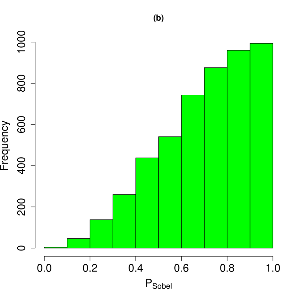
(b) The p-values of Sobel method.

Figure 4: The histogram of p-values for $(\alpha,\beta)=(0,0)$ with $\lambda_{n}=\sqrt{n}/\log(n)$.

Given that $\lambda_{n}=o(\sqrt{n})$ and as $n\rightarrow\infty$, under $H_{0}$ the asymptotic size of our proposed ASobel test for (1) is

$$\lim\limits_{n\rightarrow\infty}{Size(ASobel|H_{0})}=\delta.$$ (21)

The proof details of (21) and power analysis of ASobel test are presented in the supplemental material. The ASobel test, although superior to the conventional Sobel test, demonstrates inferior performance compared to the AJS method in numerical simulations. Consequently, our focus on hypothesis testing does not heavily emphasize the ASobel method. However, the ASobel plays a crucial role in constructing efficient confidence intervals for mediation effects, which will be presented in Section 4.

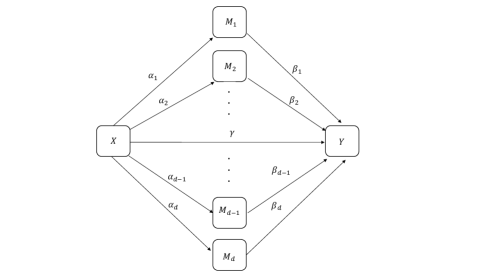
Figure 5: A scenario of mediation model with multiple mediators (confounding variables are omitted).

3 Multiple Mediation Testing with FWER Control

The proposed AJS method is extended in this section to address small-scale multiple testing with FWER control, thereby excluding the focus on high-dimensional mediators. Let $X$ be an exposure, $\mathbf{M}=(M_{1},\cdots,M_{d})^{\prime}$ be a vector of $d$-dimensional mediators, and $Y$ be an outcome of interest. Following MacKinnon (2008), it is commonly assumed that the causal relations $X\rightarrow M_{k}$ and $M_{k}\rightarrow Y$ are parameterized by $\alpha_{k}$ and $\beta_{k}$ (see Figure 5), respectively. Let $\Omega=\{k:\alpha_{k}\beta_{k}\neq 0,k=1,\cdots,d\}$ be the index set of significant (or active) mediators. Under the significance level $\delta$, we are interested in the small-scale multiple testing problem:

$$H^{(k)}_{0}:~{}\alpha_{k}\beta_{k}=0~{}~{}\leftrightarrow~{}~{}H^{(k)}_{A}:\alpha_{k}\beta_{k}\neq 0,~{}~{}k=1,\cdots,d,$$ (22)

where $d$ is not very large (i.e., the $\mathbf{M}$ is not high-dimensional), and each null hypothesis $H^{(k)}_{0}$ is composite with three components:

$$H^{(k)}_{00}:\alpha_{k}=0,\beta_{k}=0;$$

$$H^{(k)}_{10}:\alpha_{k}\neq 0,\beta_{k}=0;$$

$$H^{(k)}_{01}:\alpha_{k}=0,\beta_{k}\neq 0.$$

Denote $\Omega_{00}=\{k:H^{(k)}_{00}~{}{\rm holds},k=1,\cdots,d\}$, $\Omega_{10}=\{k:H^{(k)}_{10}~{}{\rm holds},k=1,\cdots,d\}$ and $\Omega_{01}=\{k:H^{(k)}_{01}~{}{\rm holds},k=1,\cdots,d\}$.

First we focus on extending the AJS method (in Section 2) for the multiple testing in (22). For $k=1,\cdots,d$, we denote

$$P_{\alpha_{k}}=2\{1-\Phi_{N(0,1)}(|T_{\alpha_{k}}|)\},~{}{\rm and}~{}P_{\beta_{k}}=2\{1-\Phi_{N(0,1)}(|T_{\beta_{k}}|)\},~{}k=1,\cdots,d.$$ (23)

Here $T_{\alpha_{k}}=\hat{\alpha}_{k}/\hat{\sigma}_{\alpha_{k}}$ and $T_{\beta_{k}}=\hat{\beta}_{k}/\hat{\sigma}_{\beta_{k}}$; $\hat{\alpha}_{k}$ and $\hat{\beta}_{k}$ are the estimates for $\alpha_{k}$ and $\beta_{k}$, respectively. $\hat{\sigma}_{\alpha_{k}}$ and $\hat{\sigma}_{\beta_{k}}$ are the estimated standard errors of $\hat{\alpha}_{k}$ and $\hat{\beta}_{k}$, respectively. Specifically, let

$$P^{(k)}_{JS}=\max(P_{\alpha_{k}},P_{\beta_{k}}),$$ (24)

where $P_{\alpha_{k}}$ and $P_{\beta_{k}}$ are given in (23), $k=1,\cdots,d$. We propose an AJS test method with the statistic being defined as

$$P^{(k)}_{AJS} = \left\{\begin{array}[]{ll}P^{(k)}_{JS},&\max\{|T_{\alpha_{k}}|,|T_{\beta_{k}}|\}\geq\lambda_{n},\\ \{P^{(k)}_{JS}\}^{2},&\max\{|T_{\alpha_{k}}|,|T_{\beta_{k}}|\}<\lambda_{n},\end{array}\right.$$ (27)

where $P^{(k)}_{JS}$ is given in (24), the value of $\lambda_{n}$ is equivalent to that of $P_{AJS}$ in (12). For controlling the FWER, we can reject $H^{(k)}_{0}$ if the AJS test statistic $P^{(k)}_{AJS}$ is much smaller than $\delta/d$. In other words, an estimated index set of significant mediators with AJS test is $\hat{\Omega}_{AJS}=\{k:P^{(k)}_{AJS}<\delta/d,k=1,\cdots,d\}$, where $P^{(k)}_{AJS}$ is defined in (27).

Theorem 2

Under the significance level $\delta$, with probability approaching one, the FWER of the AJS test for (22) asymptotically satisfies

$$\lim\limits_{n\rightarrow\infty}FWER(AJS)\leq\delta.$$ (28)

Remark 1

The $FWER(AJS)$ is asymptotically controlled below the significance level $\delta$ for small-scale multiple testing. However, the AJS cannot be directly applied to high-dimensional mediators, such as 450K or 850K DNA methylation markers (Zhang et al., 2016; Perera et al., 2022). In the context of large-scale mediators, advanced high-dimensional statistical techniques are necessary, which outside the scope of this paper. In this regard, we refer to the works by Zhang et al. (2016; 2021), Huang (2019), Luo et al. (2020), Liu et al. (2022), Dai et al. (2022), Perera et al. (2022) and Tian et al. (2022), among others.

Remark 2

The ASobel method can be extended in a similar manner to address the multiple testing problem presented in (22). As discussed in section 2, AJS outperforms ASobel numerically, hence this topic is not explored further in this paper.

4 Adaptive Sobel-Type Confidence Intervals

In the current section, we focus on the estimation method for confidence intervals of mediation effects $\alpha_{k}\beta_{k}$’s, which plays a crucial role in comprehending the mediation mechanism with desirable levels of confidence. The index $k$ in $\alpha_{k}\beta_{k}$ is omitted for the sake of convenience, while maintaining the same level of generality. The AJS method in Section 2 is proposed for conducting hypothesis testing, but it cannot be utilized for constructing confidence intervals of mediation effects. The Sobel-type (or normality-based) method is consistently employed in the literature to examine confidence intervals of mediation effects. To be specific, as $n\rightarrow\infty$, Sobel’s method assumes that

$$\hat{\sigma}_{\alpha\beta}^{-1}({\hat{\alpha}\hat{\beta}-\alpha\beta})\stackrel{{\scriptstyle d}}{{\longrightarrow}}N(0,1),$$ (29)

where $\stackrel{{\scriptstyle d}}{{\longrightarrow}}$ denotes convergence in distribution, $\hat{\alpha}$ and $\hat{\beta}$ are the estimates for $\alpha$ and $\beta$, respectively; $\hat{\sigma}_{\alpha}$ and $\hat{\sigma}_{\beta}$ are the estimated standard errors of $\hat{\alpha}$ and $\hat{\beta}$, respectively; $\hat{\sigma}_{\alpha\beta}=\{\hat{\alpha}^{2}\hat{\sigma}^{2}_{\beta}+\hat{\beta}^{2}\hat{\sigma}^{2}_{\alpha}\}^{1/2}$. The focus of our study lies in constructing $100(1-\delta)\%$ confidence intervals for mediation effects, where $\delta$ is commonly selected as $0.05$. Based on (29), the Sobel-typle $100(1-\delta)\%$ confidence interval for $\alpha\beta$ is given by

$${\rm CI_{Sobel}}=[\hat{\alpha}\hat{\beta}-N_{1-\delta/2}(0,1)\hat{\sigma}_{\alpha\beta},~{}\hat{\alpha}\hat{\beta}+N_{1-\delta/2}(0,1)\hat{\sigma}_{\alpha\beta}],$$ (30)

where $N_{1-\delta/2}(0,1)$ is the $(1-\delta/2)$-quantile of $N(0,1)$. However, the confidence interval ${\rm CI_{Sobel}}$ provided in (30) is excessively wide when both $\alpha$ and $\beta$ are equal to zero, resulting in a coverage probability of one for the $95\%$ confidence interval.

The asymptotic distribution of $\hat{\sigma}_{\alpha\beta}^{-1}({\hat{\alpha}\hat{\beta}-\alpha\beta})$ is $N(0,1/4)$ instead of $N(0,1)$ when $\alpha=\beta=0$, as stated in Liu et al. (2022). To amend the issue of ${\rm CI_{Sobel}}$ in the case of $\alpha=\beta=0$, we propose a novel adaptive Sobel-type (ASobel) confidence interval for $\alpha\beta$ as follows,

$${\rm CI_{ASobel}} = \left\{\begin{array}[]{ll}[\hat{\alpha}\hat{\beta}-N_{1-\delta/2}(0,1)\hat{\sigma}_{\alpha\beta},~{}\hat{\alpha}\hat{\beta}+N_{1-\delta/2}(0,1)\hat{\sigma}_{\alpha\beta}],&\max\{|T_{\alpha}|,|T_{\beta}|\}\geq\lambda_{n},\\ {[\hat{\alpha}\hat{\beta}-N_{1-\delta/2}(0,1/4)\hat{\sigma}_{\alpha\beta},~{}\hat{\alpha}\hat{\beta}+N_{1-\delta/2}(0,1/4)\hat{\sigma}_{\alpha\beta}]},&\max\{|T_{\alpha}|,|T_{\beta}|\}<\lambda_{n},\end{array}\right.$$ (32)

where $N_{1-\delta/2}(0,1/4)$ is the $(1-\delta/2)$-quantile of $N(0,1/4)$. The thresholding framework in (32) shares a similar concept with the AJS introduced in Section 2.

Theorem 3

As the sample size $n$ approaches infinity, the coverage probability of the $100(1-\delta)\%$ confidence interval given in (32) asymptotically satisfies

$$\lim_{n\rightarrow\infty}\mathbb{P}(\alpha\beta\in{\rm CI_{ASobel}})=1-\delta.$$

In what follows, we provide some comparisons between ${\rm CI_{Sobel}}$ and ${\rm CI_{ASobel}}$. The Sobel-type confidence interval can be directly derived to satisfy the following expression:

$$\lim_{n\rightarrow\infty}\mathbb{P}(\alpha\beta\in{\rm CI_{Sobel}}) = \left\{\begin{array}[]{ll}2\Phi_{N(0,1/4)}(N_{1-\delta/2}(0,1))-1,&\alpha=\beta=0,\\ 1-\delta,&others,\end{array}\right.$$

where ${\rm CI_{Sobel}}$ is given in (30). By deducing the difference between $\lim_{n\rightarrow\infty}\mathbb{P}(\alpha\beta\in{\rm CI_{Sobel}})$ and $1-\delta$ under the case of $\alpha=\beta=0$, we have

$$\lim_{n\rightarrow\infty}\mathbb{P}(\alpha\beta\in{\rm CI_{Sobel}})-(1-\delta) = 2\Phi_{N(0,1/4)}(N_{1-\delta/2}(0,1))-2+\delta$$

$$> 0.$$

Hence, the asymptotic coverage probability of ${\rm CI_{ASobel}}$ is therefore closer to $(1-\delta)$ than that of ${\rm CI_{Sobel}}$ under $\alpha=\beta=0$. Furthermore, the averaged length of ${\rm CI_{ASobel}}$ in the case of $\alpha=\beta=0$, $2N_{1-\delta/2}(0,1/4)\hat{\sigma}_{\alpha\beta}$ , is significantly shorter compared to that of ${\rm CI_{Sobel}}$, which is $2N_{1-\delta/2}(0,1)\hat{\sigma}_{\alpha\beta}$. The performance of ${\rm CI_{Sobel}}$ and ${\rm CI_{ASobel}}$ will be compared through numerical simulations.

5 Numerical Studies

5.1 Size and Power of Single-Mediator Testing

In this section, we conduct some simulations to evaluate the performance of the AJS test for $H_{0}:\alpha\beta=0$ in the context of one mediator. Under the framework of mediation analysis, we consider three kinds of outcomes with one continuous mediator: linear mediation model (continuous outcome), logistic mediation model (binary outcome) and Cox mediation model (time-to-event outcome). To make the simulation simple and focused, we do not consider any covariates in the simulation, although our method has a similar performance when handling any covariate adjustment in these models. Specifically, the mediator $M$ is generated from the linear model $M=\alpha X+e$, where $X$ and $e$ follow from $N(0,1)$. The random outcomes are generated from the following three models:

$\bullet$ Linear mediation model:  $Y=c+\gamma X+\beta M+\epsilon$, where $c=\gamma=0.5$, $X$ follows from $N(0,1)$.

$\bullet$ Logistic mediation model:  $\mathbb{P}(Y=1|X,M)=\exp(\gamma X+\beta M)/\{1+\exp(\gamma X+\beta M)\}$, where $Y\in\{0,1\}$ is the binary outcome, $X$ follows from $N(0,1)$, and $\gamma=0.5$.

$\bullet$ Cox mediation model: Let $T$ be the failure time, and $C$ be the censoring time. The observed survival time is $Y=\min(T,C)$. Following Cox (1972), the conditional hazard function of $T$ is $\lambda(t|X,M)=\lambda_{0}(t)\exp(\gamma X+\beta M)$, where $\lambda_{0}(t)=1$ is the baseline hazard function, $X$ and $M$ follow from $N(0,1)$; $\gamma=0.5$, $C$ is generated from $U(0,c_{0})$ with $c_{0}$ being chosen as a number such that the censoring rate is about $30\%$.

Table 1: The size and power of hypothesis testing with linear mediation model^‡.

	$(\alpha,\beta)$		Sobel	JS	ASobel	AJS
$n=500$	(0, 0)		0	0.0025	0.0484	0.0487
	(0, 0.5)		0.0496	0.0532	0.0496	0.0532
	(0.5, 0)		0.0486	0.0526	0.0486	0.0526
	(0.10, 0.15)		0.3582	0.5531	0.6984	0.7246
	(0.25, 0.25)		0.9993	0.9996	0.9993	0.9996
$n=1500$	(0, 0)		0	0.0022	0.0485	0.0476
	(0, 0.5)		0.0508	0.0520	0.0508	0.0520
	(0.5, 0)		0.0465	0.0474	0.0465	0.0474
	(0.10, 0.15)		0.9560	0.9701	0.9708	0.9777
	(0.25, 0.25)		1	1	1	1

Under some regularity conditions (Vanderweele and Vansteelandt, 2009; VanderWeele and Vansteelandt, 2010; VanderWeele, 2011), the product term $\alpha\beta$ can be interpreted as the causal mediating effect of $M$ along the pathway $X\rightarrow M\rightarrow Y$ for the above three mediation models (see Figure 1). For comparison, we also use the traditional Sobel and JS methods for testing $H_{0}:\alpha\beta=0$, where the significance level is $\delta$ = 0.05. All the simulation results are based on $10000$ repetitions, where the sample size is chosen as $n=500$ and 1500, respectively. In Tables 1, S.1 and S.2, we report the sizes and powers of the Sobel, JS, ASobel and AJS methods when performing mediation tests with three kinds of outcomes. As a whole, the size of our proposed AJS and ASobel are much better than those of JS and Sobel methods, respectively. For small values of $\alpha$ and $\beta$, the power of AJS is larger than that of ASobel and the conventional Sobel and JS. These numerical findings are in line with the theoretical results of Theorem 1. In Figure 6, we present the Q-Q plots of p-values under linear mediation model with $n=500$. The results depicted in Figure 6 demonstrate that the Sobel, JS, ASobel, and AJS methods accurately approximate the distribution of their respective test statistics under either $H_{10}$ or $H_{01}$. The Sobel and JS tests, however, exhibit a conservative behavior, whereas the proposed ASobel and AJS tests still accurately approximate the distribution of their corresponding test statistics. The quantiles of p-values under $H_{A}$ increase in the following order: AJS, ASobel, JS, Sobel. The aforementioned finding is consistent with the power performance presented in Table 1. The Q-Q plots of p-values under logistic and Cox mediation models demonstrate comparable performances to those illustrated in Figure 6 and are presented in Figures S.1 and S.2, respectively.

(a) Q-Q plots of p-values under $H_{00}$.

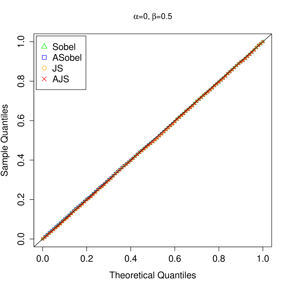
(b) Q-Q plots of p-values under $H_{01}$.

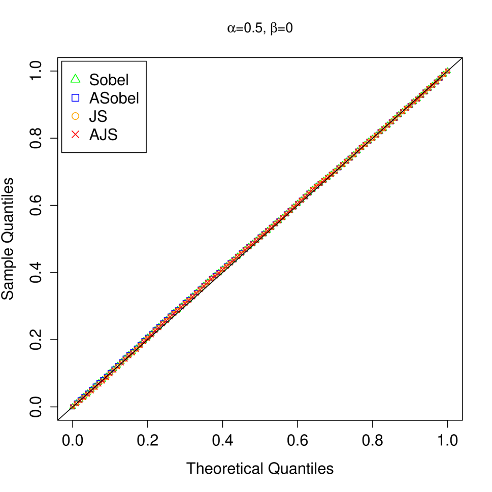
(c) Q-Q plots of p-values under $H_{10}$.

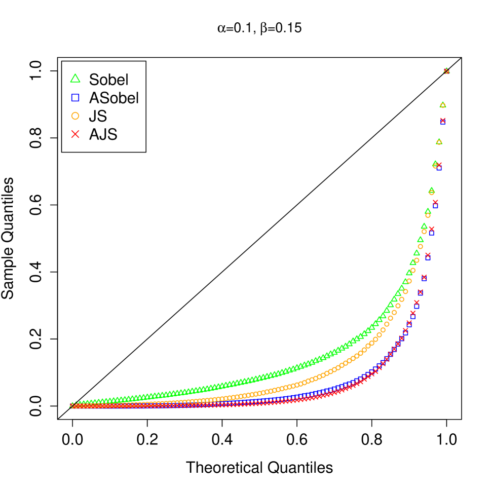
(d) Q-Q plots of p-values under $H_{A}$.

Figure 6: Q-Q plots of p-values under linear mediation model with $n=500$.

5.2 FWER and Power of Multiple-Mediators Testing

In this section, we investigate the performance of the AJS method when performing small-scale multiple testing for mediation effects via numerical simulations. The dimension of mediators is chosen as $d$ = 10, 15 and 20, respectively. Similar to Section 5.1, we consider three kinds of outcomes in the context of multiple mediators without covariates.
$\bullet$ Linear mediation model:  $Y=c+\gamma X+{\bm{\beta}}^{\prime}\mathbf{M}+\epsilon$, where $c=\gamma=0.5$, $X$ and $\epsilon$ follow from $N(0,1)$, and $\mathbf{M}=(M_{1},\cdots,M_{d})^{\prime}$ is generated from a series of linear models $M_{k}=0.5+\alpha_{k}X+e_{k}$, $k=1,\cdots,d$. Here $\mathbf{e}=(e_{1},\cdots,e_{d})^{\prime}$ is a multivariate normal vector with mean zero and covariance matrix $\Sigma=(0.25^{|i-j|})_{i,j}$. The parameter’s settings are

$${\bm{\alpha}} = (0.15,0.05,0.15,0.15,0.05,0.5,0.5,0,\cdots,0)^{\prime},$$

$${\bm{\beta}} = (0.15,0.05,0.15,0.05,0.1,0,0,0.5,0.5,0,\cdots,0)^{\prime}.$$

$\bullet$ Logistic mediation model:   $\mathbb{P}(Y=1|X,\mathbf{M})=\exp(\gamma X+{\bm{\beta}}^{\prime}\mathbf{M})/\{1+\exp(\gamma X+{\bm{\beta}}^{\prime}\mathbf{M})\}$, where $Y\in\{0,1\}$ is the binary outcome, other variables and parameters are designed as those of the linear mediation model. Moreover, we consider the following settings for model parameters,

$${\bm{\alpha}} = (0.15,0.2,0.25,0.2,0.15,0.65,0,\cdots,0)^{\prime},$$

$${\bm{\beta}} = (0.25,0.3,0.25,0.15,0.25,0,0.55,0,\cdots,0)^{\prime}.$$

$\bullet$ Cox mediation model: Given the covariate $X$ and the mediator vector $\mathbf{M}$, the Cox’s conditional hazard function of failure time $T$ is $\lambda(t|X,\mathbf{M})=\lambda_{0}(t)\exp(\gamma X+{\bm{\beta}}^{\prime}\mathbf{M})$, where $\lambda_{0}(t)=1$, $\gamma=0.5$, $X$ and $\mathbf{M}$ are generated in the same way as the linear mediation model. We generate the censoring time $C$ from $U(0,c_{0})$, where $c_{0}$ is being chosen such that the censoring rate is about $30\%$. The settings of the model’s parameters are

$${\bm{\alpha}} = (0.2,0.35,0.25,0.15,0.15,0.5,0,\cdots,0)^{\prime},$$

$${\bm{\beta}} = (0.15,0.25,0.3,0.15,0.1,0,0.5,0,\cdots,0)^{\prime},$$

The index set of significant mediators is $\Omega=\{1,2,3,4,5\}$. From Vanderweele and Vansteelandt (2009; 2010) and Huang and Yang (2017), the product term $\alpha_{k}\beta_{k}$ describes the causal mediation effect along the $k$th pathway $X\rightarrow M_{k}\rightarrow Y$ (see Figure 4), where $k=1,\cdots,d$. Note that the mediating signal of Case B is much stronger than that of Case A. Under the significance level $\delta$, we consider the multiple testing problem $H_{0k}:~{}\alpha_{k}\beta_{k}=0$, $k=1,\cdots,d$. The proposed AJS is compared with Sobel, JS, JT_Comp Huang (2019) and DACT Liu et al. (2022) in terms of empirical FWER and Power. Note that the HDMT Dai et al. (2022) is not applicable in our simulation scenarios, as it specifically targets high-dimensional mediation hypotheses with $d\rightarrow\infty$. All the results are based on 5000 repetitions, where the sample size is $n=500$ and 1500, respectively.

In Tables 2 and S.3-S.4, we report the FWERs and Powers of six test methods in the context of linear, logistic and Cox mediation models, where the significance level is $\delta=$ 0.05. The results demonstrate that the FWER and Power of AJS outperform the other five methods significantly. The powers of six methods are observed to increase with the sample size, while they decline with the increase in dimension $d$. One explanation for this phenomenon is due to the fact that the estimated variances of model parameters are becoming larger as the increase of mediator’s dimension under fixed sample size.

Table 2: The FWER and power of multiple testing with linear mediation model ($\delta=0.05$)^‡.

	Dimension		Sobel	JS	JT_Comp	DACT	AJS
$n=500$	$d=10$	FWER	0.0160	0.0216	0.1986	0.0006	0.0262
		Power	0.0464	0.1888	0.0123	0.0242	0.3332
	$d=15$	FWER	0.0108	0.0142	0.2188	0.0018	0.0308
		Power	0.0303	0.1600	0.0128	0.0648	0.2964
	$d=20$	FWER	0.0080	0.0108	0.2588	0.0088	0.0410
		Power	0.0202	0.1402	0.0172	0.1166	0.2755
$n=1500$	$d=10$	FWER	0.0176	0.0206	0.2140	0	0.0274
		Power	0.4120	0.4662	0.1241	0.0270	0.6099
	$d=15$	FWER	0.0112	0.0128	0.2310	0	0.0348
		Power	0.3976	0.4525	0.1518	0.2011	0.5886
	$d=20$	FWER	0.0124	0.0140	0.2878	0.0030	0.0438
		Power	0.3884	0.4425	0.1856	0.3392	0.5748

Table 3: The coverage probability and length of 95% confidence interval with linear mediation model^‡.

			CP				LCI
	$(\alpha_{k},\beta_{k})$		Sobel		ASobel		Sobel		ASobel
$n=500$	(0, 0)		0.9998		0.9482		0.01024		0.00513
	(0.35, 0)		0.9568		0.9568		0.06637		0.06637
	(0.5, 0)		0.9544		0.9544		0.09450		0.09450
	(0, 0.35)		0.9562		0.9562		0.06197		0.06197
	(0, 0.5)		0.9530		0.9530		0.08804		0.08804
	(0.15, 0.3)		0.9382		0.9380		0.06033		0.06027
	(0.25, 0.35)		0.9406		0.9406		0.07723		0.07723
$n=1500$	(0, 0)		0.9998		0.9466		0.00338		0.00169
	(0.35, 0)		0.9542		0.9542		0.03799		0.03799
	(0.5, 0)		0.9512		0.9512		0.05410		0.05410
	(0, 0.35)		0.9478		0.9478		0.03562		0.03562
	(0, 0.5)		0.9536		0.9536		0.05069		0.05069
	(0.15, 0.3)		0.9448		0.9448		0.03465		0.03465
	(0.25, 0.35)		0.9464		0.9464		0.04415		0.04415

${\ddagger}$ “CP” denotes the empirical coverage probability; “LCI” denotes the length of 95% confidence interval; “Sobel” denotes the ${\rm CI_{Sobel}}$ in (30); “ASobel” denotes the proposed ${\rm CI_{ASobel}}$ in (32).

5.3 Coverage Probability of Confidence Interval

The performance of the ASobel-type confidence interval presented in Section 4 is evaluated through simulations conducted in this subsection. The traditional Sobel-type confidence interval, ${\rm CI_{Sobel}}$, given in (30), is also considered for comparison. The data are generated in a similar manner as those described in Section 5.2, with the parameters chosen as (i) Linear mediation model : ${\bm{\alpha}}=(0,0.35,0.5,0,0,0.15,0.25)^{\prime}$ and ${\bm{\beta}}=(0,0,0,0.35,0.5,0.3,0.35)^{\prime}$; (ii) Logistic mediation model: ${\bm{\alpha}}=(0,0.35,0.5,0,0,0.25,0.35)^{\prime}$ and ${\bm{\beta}}=(0,0,0,0.55,0.75,0.25,0.35)^{\prime}$; (iii) Cox mediation model: ${\bm{\alpha}}=(0,0.35,0.5,0,0,0.25,0.35)^{\prime}$ and ${\bm{\beta}}=(0,0,0,0.5,0.45,0.25,0.35)^{\prime}$. The sample sizes are chosen as $n=500$ and 1500, respectively. All the results are based on 5000 repetitions.

The coverage probability (CP) and length of the 95% confidence interval (LCI) with ${\rm CI_{Sobel}}$ and ${\rm CI_{ASobel}}$ are reported in Tables 3, S.5 and S.6. The ${\rm CI_{ASobel}}$ outperforms ${\rm CI_{Sobel}}$ in terms of CP under $\alpha=\beta=0$. Additionally, the LCI of ${\rm CI_{ASobel}}$ is significantly shorter compared to that of ${\rm CI_{Sobel}}$ when $\alpha\beta=0$. These findings are consistent with the result of Theorem 3.

6 Real Data Examples

In this section, we apply our proposed AJS method for testing the mediation effects towards three real-world datasets with continuous, binary and time-to-event outcomes, respectively. The details about the three datasets and mediation analysing procedures are presented as follows:

Dataset I: (continuous outcomes). The Louisiana State University Health Sciences Center has explored the relationship between children weight and behavior through a survey of children, teachers and parents in Grenada. The dataset is publicly available within the R package mma. To perform mediation analysis as that of Yu and Li (2017), we set gender as the exposure $X$ (Male =0; Female = 1), and the outcome $Y$ is body mass index (BMI). We consider three mediators: $M_{1}$ (join in a sport team or not), $M_{2}$ (number of hours of exercises per week) and $M_{3}$ (number of hours of sweating activities per week). Furthermore, there are three covariates $Z_{1}$ (age), $Z_{2}$ (number of people in family) and $Z_{3}$ (the number of cars in family). After removing those individuals with missing data, we totally have 646 samples when conducting mediation analysis in the context of logistic mediation models. We consider the logistic mediation model to fit this dataset:

$$Y = c+\gamma X+{\bm{\beta}}^{\prime}\mathbf{M}+{\bm{\theta}}^{\prime}\mathbf{Z}+\epsilon,$$

$$M_{k} = c_{k}+\alpha_{k}X+{\bm{\eta}}_{k}^{\prime}\mathbf{Z}+e_{k},~{}~{}k=1,2,3,$$

where $Y$ is the continuous outcome, $\mathbf{M}=(M_{1},M_{2},M_{3})^{\prime}$ is the vector of mediators, $\mathbf{Z}=(Z_{1},Z_{2},Z_{3})^{\prime}$ is the vector of covariates. By VanderWeele and Vansteelandt (2010), the product term $\alpha_{k}\beta_{k}$ can be interpreted as the causal mediating effect of $M_{k}$ along the pathway $X\rightarrow M_{k}\rightarrow Y$. Here we consider the multiple testing problem $H_{0k}:~{}\alpha_{k}\beta_{k}=0$, $k=1,2,3$. The details of $P_{Sobel}$, $P_{ASobel}$$P_{JS}$ and $P_{AJS}$ are presented in Table 4. The estimators $\hat{\alpha}_{k}$’s and $\hat{\beta}_{k}$’s along with their standard errors are also given in Table 4. Particularly, $P_{AJS}\leq P_{JS}$ and $P_{ASobel}\leq P_{Sobel}$ demonstrate that the proposed AJS and ASobel are superior to traditional JS and Sobel, respectively. In Table 5, we give the 95% confidence intervals for mediation effects $\alpha_{k}\beta_{k}$’s, where ${\rm CI_{Sobel}}$ and ${\rm CI_{ASobel}}$ are defined in (30) and (32), respectively. The results from Table 5 demonstrate that the proposed adaptive Sobel-type method yields a significantly shorter and more reliable confidence interval compared to the conventional Sobel’s method.

Dataset II: (binary outcomes). The Job Search Intervention Study (JOBS II) is a randomized field experiment that investigates the efficacy of a job training intervention on unemployed workers. The dataset is publicly available within the R package mediation. Our research aims to investigate whether the workshop enhances future employment prospects by increasing job-search self-efficacy levels. To be specific, we study the mediating role of job-search self-efficacy between job-skills workshop and employment status. For this aim, we set the exposure $X$ as an indicator variable for whether participant was randomly selected for the JOBS II training program (1 = assignment to participation); the mediator $M_{1}$ is a continuous scale measuring the level of job-search self-efficacy; the outcome $Y$ is a binary measure of employment (1 = employed). Furthermore, there are 9 covariates: $Z_{1}$ (age), $Z_{2}$ (sex; 1 = female), $Z_{3}$ (level of economic hardship pre-treatment), $Z_{4}$ (measure of depressive symptoms pre-treatment), $Z_{5}$ (factor with seven categories for various occupations), $Z_{6}$ (factor with five categories for marital status), $Z_{7}$ (indicator variable for race; 1 = nonwhite), $Z_{8}$ (factor with five categories for educational attainment), $Z_{9}$ (factor with five categories for level of income). After excluding individuals with missing data, we have a total of 899 samples for conducting mediation analysis within the framework of logistic mediation models:

$$\mathbb{P}({Y}=1|X,{M}_{1},\mathbf{Z}) = \frac{\exp(c+\gamma X+\beta_{1}{M_{1}}+{\bm{\theta}}^{\prime}\mathbf{Z})}{1+\exp(c+\gamma X+\beta_{1}{M_{1}}+{\bm{\theta}}^{\prime}\mathbf{Z})},$$

$$M_{1} = c_{1}+\alpha_{1}X+{\bm{\eta}}^{\prime}\mathbf{Z}+e,$$

where $Y\in\{0,1\}$ is the binary outcome, $M_{1}$ is the mediator, $\mathbf{Z}=(Z_{1},\cdots,Z_{9})^{\prime}$ is the vector of covariates. By VanderWeele and Vansteelandt (2010), the product term $\alpha_{1}\beta_{1}$ can be interpreted as the causal mediating effect of $M_{1}$ along the pathway $X\rightarrow M_{1}\rightarrow Y$. Here we consider the mediation testing problem $H_{01}:~{}\alpha_{1}\beta_{1}=0$. The details of $P_{Sobel}$, $P_{ASobel}$, $P_{JS}$ and $P_{AJS}$ are presented in Table 4. The estimators $\hat{\alpha}_{1}$’s and $\hat{\beta}_{1}$’s along with their standard errors are also given in Table 4. It seems that the $M_{1}$ has a significant mediating role between exposure and outcome. Particularly, $P_{AJS}\leq P_{JS}$ and $P_{ASobel}\leq P_{Sobel}$ demonstrate that the proposed method works well in practical application. The 95% confidence interval of the mediation effect is presented in Table 5, which yields a similar conclusion to that of the dataset I.

Dataset III: (time-to-event outcomes). We apply our proposed method to a dataset from The Cancer Genome Atlas (TCGA) lung cancer cohort study, where the data are freely available at https://xenabrowser.net/datapages/. There are 593 patients with non-missing clinical and epigenetic information. From Luo et al. (2020) and Zhang et al. (2021), we use seven DNA methylation markers as potential mediators: $M_{1}$ (cg02178957), $M_{2}$ (cg08108679), $M_{3}$ (cg21926276), $M_{4}$ (cg26387355), $M_{5}$ (cg24200525), $M_{6}$ (cg07690349) and $M_{7}$ (cg26478297). The exposure $X$ is defined as the number of packs smoked per years, and the survival time is the outcome variable. Two hundred forty three patients died during the follow-up, and the censoring rate is 59%. We are interested in testing the mediation effects of DNA methylation markers along the pathways from smoking to survival of lung cancer patients. Four covariates are included: $Z_{1}$ (age at initial diagnosis), $Z_{2}$ (gender; male = 1, female=0), $Z_{3}$ (tumor stage; Stage I = 1, Stage II = 2, Stage III = 3, Stage IV = 4), and $Z_{4}$ (radiotherapy; yes = 1, no = 0). We use the following Cox mediation model to fit this dataset:

$$\lambda(t|X,\mathbf{M},\mathbf{Z}) = \lambda_{0}(t){\exp(\gamma X+{\bm{\beta}}^{\prime}\mathbf{M}+{\bm{\theta}}^{\prime}\mathbf{Z})}$$

$$M_{k} = c_{k}+\alpha_{k}X+{\bm{\eta}}_{k}^{\prime}\mathbf{Z}+e_{k},~{}~{}k=1,\cdots,7,$$

where $\lambda_{0}(t)$ is the baseline hazard function, $\mathbf{M}=(M_{1},\cdots,M_{7})^{\prime}$ is the vector of mediators, $\mathbf{Z}=(Z_{1},Z_{2},Z_{3},Z_{4})^{\prime}$ is the vector of covariates, $e_{k}$’s are random errors. Based on Huang and Yang (2017), the term $\alpha_{k}\beta_{k}$ is the causal mediation effect of the $k$th mediator. We consider the multiple testing $H_{0k}:~{}\alpha_{k}\beta_{k}=0$, $k=1,\cdots,7$. Table 4 presents the statistics $P_{Sobel}$, $P_{JS}$ and $P_{AJS}$, along with parameter estimates and their standard errors. In view of the fact that $P_{AJS}\leq P_{JS}$ and $P_{ASobel}\leq P_{Sobel}$, the proposed method is desirable when performing mediation analysis in practical applications. The 95% confidence intervals of the mediation effects are presented in Table 5, which supports a similar conclusion as that derived from the dataset I.

Table 4: The p-values and parameter estimates in three real-world examples.

Datasets	Mediators		$P_{Sobel}$	$P_{ASobel}$	$P_{JS}$	$P_{AJS}$	$\hat{\alpha}_{k}$($\hat{\sigma}_{\alpha_{k}}$)	$\hat{\beta}_{k}$($\hat{\sigma}_{\beta_{k}}$)
I	$M_{1}$		0.03333	0.00002	0.00359	0.00001	-0.1130 (0.0388)	-0.9822 (0.3150)
	$M_{2}$		0.25023	0.02147	0.11901	0.01416	-0.1234 (0.0791)	0.2651 (0.1557)
	$M_{3}$		0.26903	0.02706	0.19525	0.03812	0.1169 (0.0551)	0.2922 (0.2256)
II	$M_{1}$		0.21183	0.01252	0.11626	0.01352	0.0774 (0.0493)	0.1356 (0.0659)
III	$M_{1}$		0.12043	0.00190	0.02822	0.00080	-0.0129 (0.0059)	1.2816 (0.5841)
	$M_{2}$		0.02527	0.00001	0.00542	0.00003	-0.0092 (0.0024)	-2.8537 (1.0262)
	$M_{3}$		0.10093	0.10093	0.08030	0.08030	-0.0094 (0.0054)	-3.4795 (0.7357)
	$M_{4}$		0.10074	0.00103	0.02692	0.00072	-0.0125 (0.0051)	-1.4994 (0.6776)
	$M_{5}$		0.15777	0.15777	0.13013	0.13013	-0.0033 (0.0022)	6.2711 (1.5944)
	$M_{6}$		0.05167	0.00010	0.02247	0.00051	-0.0162 (0.0071)	1.9535 (0.5246)
	$M_{7}$		0.08990	0.00069	0.05725	0.00328	-0.0256 (0.0068)	-0.8417 (0.4426)

Table 5: The 95% confidence intervals for mediation effects in three real-world examples.

Datasets	Mediators		${\rm CI_{Sobel}}$		${\rm CI_{ASobel}}$		$\hat{\alpha}_{k}\hat{\beta}_{k}$
I	$M_{1}$		[0.00877, 0.21325]		[0.05989, 0.16213]		0.11099
	$M_{2}$		[$-$0.08847, 0.02305]		[$-$0.06058, $-$0.00483]		$-$0.03271
	$M_{3}$		[$-$0.02641, 0.09471]		[0.00387, 0.06443]		0.03416
II	$M_{1}$		[$-$0.00598, 0.02697]		[0.00226, 0.01873]		0.01049
III	$M_{1}$		[$-$0.03753, 0.00435]		[$-$0.02707, $-$0.00612]		$-$0.01659
	$M_{2}$		[0.00325, 0.04912]		[0.01471, 0.03765]		0.02617
	$M_{3}$		[$-$0.00635, 0.07154]		[$-$0.00635, 0.07154]		0.03260
	$M_{4}$		[$-$0.00363, 0.04097]		[0.00752, 0.02982]		0.01868
	$M_{5}$		[$-$0.04995, 0.00811]		[$-$0.04995, 0.00811]		$-$0.02095
	$M_{6}$		[$-$0.06349, 0.00023]		[$-$0.04756, $-$0.01570]		$-$0.03163
	$M_{7}$		[$-$0.00335, 0.04642]		[0.00909, 0.03398]		0.02154

7 Concluding Remarks

In this paper, we have proposed an data-adaptive joint significance mediation effects test procedure. The explicit expressions of size and power were derived. We also have extended the AJS for performing small-scale multiple testing with FWER control. An adaptive Sobel-type confidence interval was presented. Some simulations and three real-world examples were used to illustrate the usefulness of our method. The focus of this study was limited to a single mediator or a small number of mediators, and the inclusion of high-dimensional mediators was beyond the scope of this research. The following papers are recommended for those interested in high-dimensional mediation analysis, including Zhang et al. (2016; 2021), Luo et al. (2020), Perera et al. (2022) and Tian et al. (2022), among others.

There exist two possible directions for applying the proposed AJS test method in our future research. (i) Microbiome Mediation Analysis. Recently, increasing studies have studied the biological mechanisms whether the microbiome play a mediating role between an exposure and a clinical outcome (Sohn and Li, 2019; Wang et al., 2020; Zhang et al., 2021; Sohn et al., 2022; Yue and Hu, 2022). For improving the powers of mediation effect testing, it is desirable to use the AJS test method when performing microbiome mediation analysis. (ii) Multiple-Mediator Testing with FDR control. We have studied the theoretical and numerical performances of AJS test method for multiple testing with FWER control. Following Sampson et al. (2018), it is useful to investigate the AJS test for multiple mediators with FDR control in some applications.

Appendix A Proofs

In this section, we give the proof details of Theorems 1-3.

Proof of Theorem 1. Under $H_{00}$, the size of the AJS test is determined by

$$Size(AJS|H_{00}) = \mathbb{P}(P_{AJS}<\delta|H_{00})$$

$$= \mathbb{P}(P_{AJS}<\delta,T_{max}\geq\lambda_{n}|H_{00})+\mathbb{P}(P_{AJS}<\delta,T_{max}>\lambda_{n}|H_{00})$$

$$= \mathbb{P}(T_{max}\geq\lambda_{n}|H_{00})\mathbb{P}(P_{AJS}<\delta|T_{max}\geq\lambda_{n},H_{00})$$

$$+~{}\mathbb{P}(T_{max}<\lambda_{n}|H_{00})\mathbb{P}(P_{AJS}<\delta|T_{max}<\lambda_{n},H_{00}),$$

where $T_{max}=\max\{|T_{\alpha}|,|T_{\beta}|\}$. As $n\rightarrow\infty$, it follows from the definition of $P_{AJS}$ that

$$\mathbb{P}(P_{AJS}<\delta|T_{max}\geq\lambda_{n},H_{00}) = \mathbb{P}(P_{JS}<\delta|H_{00})$$

$$= \mathbb{P}(P_{\alpha}<\delta|H_{00})\mathbb{P}(P_{\beta}<\delta|H_{00})$$

$$= \delta^{2}.$$

Here the last equality is due to the fact that $P_{\alpha}$ and $P_{\beta}$ independently follow from $U(0,1)$ under $H_{00}$. The distribution of $P_{JS}^{2}$ being $U(0,1)$ under $H_{00}$ allows us to deduce that

$$\mathbb{P}(P_{AJS}<\delta|T_{max}<\lambda_{n},H_{00}) = \mathbb{P}(P_{JS}^{2}<\delta|H_{00})$$

$$= \delta.$$

Under $H_{00}$, we know that $\lim_{n\rightarrow\infty}\mathbb{P}(T_{max}\geq\lambda_{n}|H_{00})=0$ and $\lim_{n\rightarrow\infty}\mathbb{P}(T_{max}<\lambda_{n}|H_{00})=1$. The equations (A), (A) and (A) imply that the asymptotic size of AJS given $H_{00}$ is equal to $\delta$.

Under $H_{10}$, the size of the AJS test is denoted as

$$Size(AJS|H_{10}) = \mathbb{P}(P_{AJS}<\delta|H_{10})$$

$$= \mathbb{P}(P_{AJS}<\delta,T_{max}\geq\lambda_{n}|H_{10})+\mathbb{P}(P_{AJS}<\delta,T_{max}<\lambda_{n}|H_{10})$$

$$= \mathbb{P}(T_{max}\geq\lambda_{n}|H_{10})\mathbb{P}(P_{AJS}<\delta|T_{max}\geq\lambda_{n},H_{10})$$

$$+~{}\mathbb{P}(T_{max}<\lambda_{n}|H_{10})\mathbb{P}(P_{AJS}<\delta|T_{max}<\lambda_{n},H_{10}).$$

Under $H_{10}$, as $n\rightarrow\infty$ we can derive that

$$\mathbb{P}(P_{AJS}<\delta|T_{max}\geq\lambda_{n},H_{10}) = \mathbb{P}(P_{JS}<\delta|H_{10})$$

$$= \mathbb{P}(P_{\beta}<\delta|H_{10})$$

$$= \delta,$$

and

$$\mathbb{P}(P_{AJS}<\delta|T_{max}<\lambda_{n},H_{10}) = \mathbb{P}(P_{JS}^{2}<\delta|H_{10})$$

$$= \mathbb{P}(P_{\beta}<\sqrt{\delta}|H_{10})$$

$$= \sqrt{\delta}.$$

In view of (A), (A) and (A), we have

$$Size(AJS|H_{10}) = \delta\mathbb{P}(T_{max}\geq\lambda_{n}|H_{10})+\sqrt{\delta}\mathbb{P}(T_{max}<\lambda_{n}|H_{10})$$

$$= \delta+\Delta_{AJS|H_{10}},$$

where $\Delta_{AJS|H_{10}}=(\sqrt{\delta}-\delta)\mathbb{P}\big{(}T_{max}<\lambda_{n}|H_{10}\big{)}$. As $n\rightarrow\infty$, $\Delta_{AJS|H_{10}}=o_{P}(1)$ due to $\lim_{n\rightarrow\infty}\mathbb{P}\big{(}T_{max}<\lambda_{n}|H_{10}\big{)}=0$. Therefore,

$$\lim\limits_{n\rightarrow\infty}{Size(AJS|H_{10})} = \delta.$$

In a similar way, under $H_{01}$ we can obtain the size of the AJS test is $Size(AJS|H_{01})=\delta+\Delta_{AJS|H_{01}}$, where $\Delta_{AJS|H_{01}}=(\sqrt{\delta}-\delta)\mathbb{P}\big{(}T_{max}<\lambda_{n}|H_{01}\big{)}=o_{P}(1)$ as $n\rightarrow\infty$. Hence,

$$\lim\limits_{n\rightarrow\infty}{Size(AJS|H_{01})} = \delta.$$

Finally, under $H_{A}$ the power of AJS test is written as

$$Power(AJS) = \mathbb{P}(P_{AJS}<\delta|H_{A})$$

$$= \mathbb{P}(P_{AJS}<\delta,T_{max}\geq\lambda_{n}|H_{A})+\mathbb{P}(P_{AJS}<\delta,T_{max}<\lambda_{n}|H_{A})$$

$$= \mathbb{P}(T_{max}\geq\lambda_{n}|H_{A})\mathbb{P}(P_{AJS}<\delta|T_{max}\geq\lambda_{n},H_{A})$$

$$+~{}\mathbb{P}(T_{max}<\lambda_{n}|H_{A})\mathbb{P}(P_{AJS}<\delta|T_{max}<\lambda_{n},H_{A}).$$

Under $H_{A}$, it is straightforward to deduce that

$$\mathbb{P}(P_{\alpha}<\delta|H_{A}) = \mathbb{P}\big{(}2\{1-\Phi_{N(0,1)}(|T_{\alpha}|)\}<\delta|H_{A}\big{)}$$

$$= \mathbb{P}(|T_{\alpha}|>N_{1-\alpha/2}(0,1)|H_{A})$$

$$= \Phi_{N(0,1)}\big{(}\mu_{\alpha}-N_{1-\delta/2}(0,1)\big{)}+\Phi_{N(0,1)}\big{(}-\mu_{\alpha}-N_{1-\delta/2}(0,1)\big{)},$$

and

$$\mathbb{P}(P_{\beta}<\delta|H_{A}) = \Phi_{N(0,1)}\big{(}\mu_{\beta}-N_{1-\delta/2}(0,1)\big{)}+\Phi_{N(0,1)}\big{(}-\mu_{\beta}-N_{1-\delta/2}(0,1)\big{)},$$

where $\mu_{\alpha}=\mathbb{E}(\hat{\alpha}/\hat{\sigma}_{\alpha})$ and $\mu_{\beta}=\mathbb{E}(\hat{\beta}/\hat{\sigma}_{\beta})$. Therefore,

$$Power\big{(}AJS|T_{max}\geq\lambda_{n}\big{)} \equiv \mathbb{P}(P_{AJS}<\delta|T_{max}\geq\lambda_{n},H_{A})$$

$$= \mathbb{P}(P_{\alpha}<\delta|H_{A})\mathbb{P}(P_{\beta}<\delta|H_{A})$$

$$= [\Phi_{N(0,1)}\big{(}\mu_{\alpha}-N_{1-\delta/2}(0,1)\big{)}+\Phi_{N(0,1)}\big{(}-\mu_{\alpha}-N_{1-\delta/2}(0,1)\big{)}]$$

$$\times[\Phi_{N(0,1)}\big{(}\mu_{\beta}-N_{1-\delta/2}(0,1)\big{)}+\Phi_{N(0,1)}\big{(}-\mu_{\beta}-N_{1-\delta/2}(0,1)\big{)}],$$

and

$$Power\big{(}AJS|T_{max}<\lambda_{n}\big{)} \equiv \mathbb{P}(P_{AJS}<\delta|T_{max}<\lambda_{n},H_{A})$$

$$= \mathbb{P}(P_{\alpha}<\sqrt{\delta}|H_{A})\mathbb{P}(P_{\beta}<\sqrt{\delta}|H_{A})$$

$$= [\Phi_{N(0,1)}\big{(}\mu_{\alpha}-N_{1-\sqrt{\delta}/2}(0,1)\big{)}+\Phi_{N(0,1)}\big{(}-\mu_{\alpha}-N_{1-\sqrt{\delta}/2}(0,1)\big{)}]$$

$$\times[\Phi_{N(0,1)}\big{(}\mu_{\beta}-N_{1-\sqrt{\delta}/2}(0,1)\big{)}+\Phi_{N(0,1)}\big{(}-\mu_{\beta}-N_{1-\sqrt{\delta}/2}(0,1)\big{)}].$$

The power of the AJS is established based on (A), (A) and (A). This completes the proof.

Proof of Theorem 2. For the multiple testing problem, we deduce the FWER of our proposed AJS method under the significance level $\delta$. By the definition of FWER, we can derive that

$$FWER(AJS)=\mathbb{P}\left(\bigcup_{k=1}^{d}\left\{P_{AJS}^{(k)}<\delta/d\right\}~{}\vline~{}H_{0}^{(k)},k=1,\cdots,d\right)$$

$$\leq\sum_{k=1}^{d}\mathbb{P}\left(P_{AJS}^{(k)}<\delta/d~{}\vline~{}H_{0}^{(k)}\right)$$

$$=\sum_{k\in\Omega_{00}}\mathbb{P}\left(P_{AJS}^{(k)}<\delta/d~{}\vline~{}H_{00}^{(k)}\right)+\sum_{k\in\Omega_{10}}\mathbb{P}\left(P_{AJS}^{(k)}<\delta/d~{}\vline~{}H_{10}^{(k)}\right)+\sum_{k\in\Omega_{01}}\mathbb{P}\left(P_{AJS}^{(k)}<\delta/d~{}\vline~{}H_{01}^{(k)}\right),$$

where $\Omega_{00}=\{k:H^{(k)}_{00},k=1,\cdots,d\}$, $\Omega_{10}=\{k:H^{(k)}_{10},k=1,\cdots,d\}$ and $\Omega_{01}=\{k:H^{(k)}_{01},k=1,\cdots,d\}$. In view of the fact that

$$\sum_{k\in\Omega_{00}}\mathbb{P}\left(P_{AJS}^{(k)}<\delta/d~{}\vline~{}H_{00}^{(k)}\right)=R_{1}+R_{2},$$ (S.10)

where

$${R_{1}} = {\sum_{k\in\Omega_{00}}\mathbb{P}\left(P_{AJS}^{(k)}<\delta/d,T_{max,k}\geq\lambda_{n}~{}\vline~{}H_{00}^{(k)}\right)},$$

$${R_{2}} = {\sum_{k\in\Omega_{00}}\mathbb{P}\left(P_{AJS}^{(k)}<\delta/d,T_{max,k}<\lambda_{n}~{}\vline~{}H_{00}^{(k)}\right)},$$

where $T_{max,k}=\max(|T_{\alpha_{k}}|,|T_{\beta_{k}}|)$. The term $R_{1}$ satisfies the following expression:

$$R_{1} = \sum_{k\in\Omega_{00}}\mathbb{P}\left(T_{max,k}\geq\lambda_{n}~{}\vline~{}H_{00}^{(k)}\right)\mathbb{P}\left(P_{AJS}^{(k)}<\delta/d~{}\vline~{}T_{max,k}\geq\lambda_{n},H_{00}^{(k)}\right)$$ (S.11)

$$= \sum_{k\in\Omega_{00}}\mathbb{P}\left(T_{max,k}\geq\lambda_{n}~{}\vline~{}H_{00}^{(k)}\right)\mathbb{P}\left(\{P_{JS}^{(k)}\}^{2}<\delta^{2}/d^{2}~{}\vline~{}H_{00}^{(k)}\right)$$

$$= \frac{\delta^{2}}{d^{2}}\sum_{k\in\Omega_{00}}\mathbb{P}\left(T_{max,k}\geq\lambda_{n}~{}\vline~{}H_{00}^{(k)}\right).$$

In addition,

$$R_{2} = \sum_{k\in\Omega_{00}}\mathbb{P}\left(T_{max,k}<\lambda_{n}~{}\vline~{}H_{00}^{(k)}\right)\mathbb{P}\left(P_{AJS}^{(k)}<\delta/d~{}\vline~{}T_{max,k}<\lambda_{n},H_{00}^{(k)}\right)$$ (S.12)

$$= \sum_{k\in\Omega_{00}}\mathbb{P}\left(T_{max,k}<\lambda_{n}~{}\vline~{}H_{00}^{(k)}\right)\mathbb{P}\left(\{P_{JS}^{(k)}\}^{2}<\delta/d~{}\vline~{}H_{00}^{(k)}\right)$$

$$= |\Omega_{00}|\frac{\delta}{d}-\frac{\delta}{d}\sum_{k\in\Omega_{00}}\mathbb{P}\left(T_{max,k}\geq\lambda_{n}~{}\vline~{}H_{00}^{(k)}\right).$$

Hence, it follows from (S.10), (S.11) and (S.12) that

$$\sum_{k\in\Omega_{00}}\mathbb{P}\left(P_{AJS}^{(k)}<\delta/d~{}\vline~{}H_{00}^{(k)}\right) = |\Omega_{00}|\frac{\delta}{d}+\left(\frac{\delta^{2}}{d^{2}}-\frac{\delta}{d}\right)\sum_{k\in\Omega_{00}}\mathbb{P}\left(T_{max,k}\geq\lambda_{n}~{}\vline~{}H_{00}^{(k)}\right)$$ (S.13)

$$= |\Omega_{00}|\frac{\delta}{d}+o_{P}(1),$$

where the last equality is due to $\lim_{n\rightarrow\infty}\mathbb{P}(T_{max,k}\geq\lambda_{n}~{}\vline~{}H_{00}^{(k)})=0$.

Next, we focus on the upper bound of $\sum_{k=1}^{d}\mathbb{P}\left(P_{AJS}^{(k)}<\delta/d~{}\vline~{}H_{10}^{(k)}\right)$ to control the FWER. To be specific,

$$\sum_{k\in\Omega_{10}}\mathbb{P}\left(P_{AJS}^{(k)}<\delta/d~{}\vline~{}H_{10}^{(k)}\right)=R_{3}+R_{4},$$ (S.14)

where

$${R_{3}} = {\sum_{k\in\Omega_{10}}\mathbb{P}\left(P_{AJS}^{(k)}<\delta/d,T_{max,k}\geq\lambda_{n}~{}\vline~{}H_{10}^{(k)}\right)},$$

$${R_{4}} = {\sum_{k\in\Omega_{10}}\mathbb{P}\left(P_{AJS}^{(k)}<\delta/d,T_{max,k}<\lambda_{n}~{}\vline~{}H_{10}^{(k)}\right)}.$$

Some direct deductions lead to that

$$R_{3} = \sum_{k\in\Omega_{10}}\mathbb{P}\left(T_{max,k}\geq\lambda_{n}~{}\vline~{}H_{10}^{(k)}\right)\mathbb{P}\left(P_{AJS}^{(k)}<\delta/d~{}\vline~{}T_{max,k}\geq\lambda_{n},H_{10}^{(k)}\right)$$ (S.15)

$$= \sum_{k\in\Omega_{10}}\mathbb{P}\left(T_{max,k}\geq\lambda_{n}~{}\vline~{}H_{10}^{(k)}\right)\mathbb{P}\left(P_{JS}^{(k)}<\delta/d~{}\vline~{}H_{10}^{(k)}\right)$$

$$= \frac{\delta}{d}\sum_{k\in\Omega_{10}}\mathbb{P}\left(T_{max,k}\geq\lambda_{n}~{}\vline~{}H_{10}^{(k)}\right),$$

and

$$R_{4} = \sum_{k\in\Omega_{10}}\mathbb{P}\left(T_{max,k}<\lambda_{n}~{}\vline~{}H_{10}^{(k)}\right)\mathbb{P}\left(P_{AJS}^{(k)}<\delta/d~{}\vline~{}T_{max,k}<\lambda_{n},H_{10}^{(k)}\right)$$ (S.16)

$$= \sum_{k\in\Omega_{10}}\mathbb{P}\left(T_{max,k}<\lambda_{n}~{}\vline~{}H_{10}^{(k)}\right)\mathbb{P}\left(\{P_{JS}^{(k)}\}^{2}<\delta/d~{}\vline~{}H_{10}^{(k)}\right)$$

$$= \sqrt{\frac{\delta}{d}}\sum_{k\in\Omega_{10}}\mathbb{P}\left(T_{max,k}<\lambda_{n}~{}\vline~{}H_{10}^{(k)}\right).$$

Based on (S.14), (S.15) and (S.16), we have

$$\sum_{k\in\Omega_{10}}\mathbb{P}\left(P_{AJS}^{(k)}<\delta/d~{}\vline~{}H_{10}^{(k)}\right) = \frac{\delta}{d}\left\{\sum_{k\in\Omega_{10}}\mathbb{P}\left(T_{max,k}\geq\lambda_{n}~{}\vline~{}H_{10}^{(k)}\right)\right\}$$

$$+~{}\sqrt{\frac{\delta}{d}}\left\{\sum_{k\in\Omega_{10}}\mathbb{P}\left(T_{max,k}<\lambda_{n}~{}\vline~{}H_{10}^{(k)}\right)\right\}$$

$$= |\Omega_{10}|\frac{\delta}{d}+\Delta_{AJS},$$

where

$$\Delta_{AJS}=\left(\sqrt{\frac{\delta}{d}}-\frac{\delta}{d}\right)\left\{\sum_{k\in\Omega_{10}}\mathbb{P}\left(T_{max,k}<\lambda_{n}~{}\vline~{}H_{10}^{(k)}\right)\right\}.$$

Under $H_{10}^{(k)}$, it is demonstrated that $\mathbb{P}(T_{max,k}<\lambda_{n}|H_{10}^{(k)})=o(1)$ as $n\rightarrow\infty$. This together with the boundedness of term $|\Omega_{10}|$ can ensure that $\Delta_{AJS}$ is also asymptotically negligible. i.e., $\sum_{k\in\Omega_{10}}\mathbb{P}(P_{AJS}^{(k)}<\delta/d~{}|~{}H_{10}^{(k)})=|\Omega_{10}|{\delta}/{d}+o_{P}(1)$ as $n\rightarrow\infty$. In a similar procedure, it can be demonstrated that $\sum_{k\in\Omega_{01}}\mathbb{P}(P_{AJS}^{(k)}<\delta/d~{}|~{}H_{01}^{(k)})=|\Omega_{01}|{\delta}/{d}+o_{P}(1)$. Therefore, as $n\rightarrow\infty$, the asymptotic bound of AJS’s FWER is

$$FWER(AJS) \leq |\Omega_{00}|\frac{\delta}{d}+|\Omega_{10}|\frac{\delta}{d}+|\Omega_{01}|\frac{\delta}{d}$$

$$= \delta,$$

where the last equality is due to $|\Omega_{00}|+|\Omega_{10}|+|\Omega_{01}|=d$. This completes the proof.

Proof of Theorem 3. It follows from the definition of ASobel-type confidence interval that

$$\mathbb{P}(\alpha\beta\in{\rm CI_{ASobel}}|\alpha=\beta=0)$$ (S.17)

$$=\mathbb{P}(\alpha\beta\in{\rm CI_{ASobel}},T_{max}\geq\lambda_{n}|\alpha=\beta=0)+\mathbb{P}(\alpha\beta\in{\rm CI_{ASobel}},T_{max}<\lambda_{n}|\alpha=\beta=0)$$

$$=\mathbb{P}(T_{max}\geq\lambda_{n}|\alpha=\beta=0)\mathbb{P}(\alpha\beta\in{\rm CI_{ASobel}}|T_{max}\geq\lambda_{n},\alpha=\beta=0)$$

$$+~{}\mathbb{P}(T_{max}<\lambda_{n}|\alpha=\beta=0)\mathbb{P}(\alpha\beta\in{\rm CI_{ASobel}}|T_{max}<\lambda_{n},\alpha=\beta=0),$$

where $T_{max}=\max(|T_{\alpha}|,|T_{\beta}|)$ satisfying $\lim_{n\rightarrow\infty}\mathbb{P}(T_{max}\geq\lambda_{n}|H_{00})=0$ and $\lim_{n\rightarrow\infty}\mathbb{P}(T_{max}<\lambda_{n}|H_{00})=1$. From the definition of ${\rm CI_{ASobel}}$, it is straightforward to derive the following expressions:

$$\mathbb{P}\left(\alpha\beta\in{\rm CI_{ASobel}}|T_{max}\geq\lambda_{n},\alpha=\beta=0\right) = 1-\mathbb{P}(|T_{Sobel}|>N_{1-\delta/2}(0,1)|\alpha=\beta=0)$$ (S.18)

$$= 2\Phi_{N(0,1/4)}(N_{1-\delta/2}(0,1))-1,$$

and

$$\mathbb{P}(\alpha\beta\in{\rm CI_{ASobel}}|T_{max}<\lambda_{n},\alpha=\beta=0) = 1-\mathbb{P}(|T_{Sobel}|>N_{1-\delta/2}(0,1/4)|\alpha=\beta=0)$$ (S.19)

$$= 1-\delta,$$

where $T_{Sobel}=(\hat{\alpha}\hat{\beta}-\alpha\beta)/\hat{\sigma}_{\alpha\beta}$, $\Phi_{N(0,1/4)}(\cdot)$ is the cumulative distribution function of $N(0,1/4)$, and $N_{1-\delta/2}(0,1/4)$ denotes the $(1-\delta/2)$-quantile of $N(0,1/4)$. From (S.17), (S.18) and (S.19), we can derive that

$$\lim_{n\rightarrow\infty}\mathbb{P}(\alpha\beta\in{\rm CI_{ASobel}}|\alpha=\beta=0)=1-\delta.$$

Next, we derive the asymptotic coverage probability of ${\rm CI_{ASobel}}$ under $\alpha=0,\beta\neq 0$. Note that

$$\mathbb{P}(\alpha\beta\in{\rm CI_{ASobel}}|\alpha=0,\beta\neq 0)$$ (S.20)

$$=\mathbb{P}(\alpha\beta\in{\rm CI_{ASobel}},T_{max}\geq\lambda_{n}|\alpha=0,\beta\neq 0)+\mathbb{P}(\alpha\beta\in{\rm CI_{ASobel}},T_{max}<\lambda_{n}|\alpha=0,\beta\neq 0)$$

$$=\mathbb{P}(T_{max}\geq\lambda_{n}|\alpha=0,\beta\neq 0)\mathbb{P}(\alpha\beta\in{\rm CI_{ASobel}}|T_{max}\geq\lambda_{n},\alpha=0,\beta\neq 0)$$

$$+~{}\mathbb{P}(T_{max}<\lambda_{n}|\alpha=0,\beta\neq 0)\mathbb{P}(\alpha\beta\in{\rm CI_{ASobel}}|T_{max}<\lambda_{n},\alpha=0,\beta\neq 0).$$

Some calculations lead to that

$$\mathbb{P}(\alpha\beta\in{\rm CI_{ASobel}}|T_{max}\geq\lambda_{n},\alpha=0,\beta\neq 0) = 1-\mathbb{P}(|T_{Sobel}|>N_{1-\delta/2}(0,1)|\alpha=0,\beta\neq 0)$$ (S.21)

$$= 1-\delta,$$

together with

$$\lim_{n\rightarrow\infty}\mathbb{P}(T_{max}\geq\lambda_{n}|\alpha=0,\beta\neq 0)=1-\lim_{n\rightarrow\infty}\mathbb{P}(T_{max}<\lambda_{n}|\alpha=0,\beta\neq 0)=1.$$ (S.22)

In view of (S.20), (S.21) and (S.22), under $\alpha=0,\beta\neq 0$ we can rewrite the asymptotic coverage probability of ${\rm CI_{ASobel}}$ as

$$\lim_{n\rightarrow\infty}\mathbb{P}(\alpha\beta\in{\rm CI_{ASobel}}|\alpha=0,\beta\neq 0) = 1-\delta.$$

In a similar way, it can be deduced that $\lim_{n\rightarrow\infty}\mathbb{P}(\alpha\beta\in{\rm CI_{ASobel}}|\alpha\neq 0,\beta=0)=1-\delta.$

Lastly, we focus on deducing the asymptotic coverage probability of ${\rm CI_{ASobel}}$ under $\alpha\neq 0,\beta\neq 0$. Specifically, we can derive that

$$\mathbb{P}(\alpha\beta\in{\rm CI_{ASobel}}|\alpha\neq 0,\beta\neq 0)$$ (S.23)

$$=\mathbb{P}(\alpha\beta\in{\rm CI_{ASobel}},T_{max}\geq\lambda_{n}|\alpha\neq 0,\beta\neq 0)+\mathbb{P}(\alpha\beta\in{\rm CI_{ASobel}},T_{max}<\lambda_{n}|\alpha\neq 0,\beta\neq 0)$$

$$=\mathbb{P}(T_{max}\geq\lambda_{n}|\alpha\neq 0,\beta\neq 0)\mathbb{P}(\alpha\beta\in{\rm CI_{ASobel}}|T_{max}\geq\lambda_{n},\alpha\neq 0,\beta\neq 0)$$

$$+~{}\mathbb{P}(T_{max}<\lambda_{n}|\alpha\neq 0,\beta\neq 0)\mathbb{P}(\alpha\beta\in{\rm CI_{ASobel}}|T_{max}<\lambda_{n},\alpha\neq 0,\beta\neq 0),$$

where

$$\mathbb{P}(\alpha\beta\in{\rm CI_{ASobel}}|T_{max}\geq\lambda_{n},\alpha\neq 0,\beta\neq 0) = 1-\mathbb{P}(|T_{Sobel}|>N_{1-\delta/2}(0,1)|\alpha\neq 0,\beta\neq 0)$$ (S.24)

$$= 1-\delta,$$

and

$$\lim_{n\rightarrow\infty}\mathbb{P}(T_{max}\geq\lambda_{n}|\alpha\neq 0,\beta\neq 0)=1-\lim_{n\rightarrow\infty}\mathbb{P}(T_{max}<\lambda_{n}|\alpha\neq 0,\beta\neq 0)=1.$$ (S.25)

It follows from (S.23), (S.24) and (S.25) that $\lim_{n\rightarrow\infty}\mathbb{P}(\alpha\beta\in{\rm CI_{ASobel}}|\alpha\neq 0,\beta\neq 0)=1-\delta.$ This ends the proof.

Appendix B Size and Power of the ASobel Test

In this section, we provide some details on the size and power of the ASobel test. First we deduce the size of our proposed ASobel test method under $H_{00}$. It follows from the decision rule of the ASobel test that

$$Size(ASobel|H_{00}) = \mathbb{P}(P_{ASobel}<\delta|H_{00})$$

$$= \mathbb{P}(P_{ASobel}<\delta,T_{max}<\lambda_{n}|H_{00})+\mathbb{P}(P_{ASobel}<\delta,T_{max}\geq\lambda_{n}|H_{00})$$

$$= \mathbb{P}(T_{max}<\lambda_{n}|H_{00})\mathbb{P}(P_{ASobel}<\delta|T_{max}<\lambda_{n},H_{00})$$

$$+~{}\mathbb{P}(T_{max}\geq\lambda_{n}|H_{00})\mathbb{P}(P_{ASobel}<\delta|T_{max}\geq\lambda_{n},H_{00}),$$

where $T_{max}=\max(|T_{\alpha}|,|T_{\beta}|)$. Under $H_{00}$, we have $\lim_{n\rightarrow\infty}\mathbb{P}(T_{max}\geq\lambda_{n}|H_{00})=0$ and $\lim_{n\rightarrow\infty}\mathbb{P}(T_{max}<\lambda_{n}|H_{00})=1$. From the definition of $P_{ASobel}$, it is straightforward to derive the following expressions:

$$\mathbb{P}(P_{ASobel}<\delta|T_{max}\geq\lambda_{n},H_{00}) = \mathbb{P}\Big{(}2\{1-\Phi_{N(0,1)}(|T_{Sobel}|)\}<\delta|H_{00}\Big{)}$$ (S.27)

$$= \mathbb{P}(|T_{Sobel}|>N_{1-\delta/2}(0,1)|H_{00})$$

$$= 2\{1-\Phi_{N(0,1/4)}(N_{1-\delta/2}(0,1))\},$$

and

$$\mathbb{P}(P_{ASobel}<\delta|T_{max}<\lambda_{n},H_{00}) = \mathbb{P}\Big{(}2\{1-\Phi_{N(0,1/4)}(|T_{Sobel}|)\}<\delta|H_{00}\Big{)}$$ (S.28)

$$= \mathbb{P}(|T_{Sobel}|>N_{1-\delta/2}(0,1/4)|H_{00})$$

$$= \delta,$$

where $\Phi_{N(0,1/4)}(\cdot)$ is the cumulative distribution function of $N(0,1/4)$, and $N_{1-\delta/2}(0,1/4)$ denotes the $(1-\delta/2)$-quantile of $N(0,1/4)$. From (B), (S.27) and (S.28), we can derive that

$$\lim_{n\rightarrow\infty}Size(ASobel|H_{00})=\delta.$$

Under $H_{10}$, we have

$$Size(ASobel|H_{10}) = \mathbb{P}(P_{ASobel}<\delta|H_{10})$$

$$= \mathbb{P}(P_{ASobel}<\delta,T_{max}\geq\lambda_{n}|H_{10})+\mathbb{P}(P_{ASobel}<\delta,T_{max}<\lambda_{n}|H_{10})$$

$$= \mathbb{P}(T_{max}\geq\lambda_{n}|H_{10})\mathbb{P}(P_{ASobel}<\delta|T_{max}\geq\lambda_{n},H_{10})$$

$$+~{}\mathbb{P}(T_{max}<\lambda_{n}|H_{10})\mathbb{P}(P_{ASobel}<\delta|T_{max}<\lambda_{n},H_{10}).$$

Some calculations lead to that

$$\mathbb{P}(P_{ASobel}<\delta|T_{max}\geq\lambda_{n},H_{10}) = \mathbb{P}\Big{(}2\{1-\Phi_{N(0,1)}(|T_{Sobel}|)\}<\delta|H_{10}\Big{)}$$ (S.30)

$$= \mathbb{P}(|T_{Sobel}|>N_{1-\delta/2}(0,1)|H_{10})$$

$$= \delta,$$

together with

$$\mathbb{P}(P_{ASobel}<\delta|T_{max}<\lambda_{n},H_{10}) = \mathbb{P}\Big{(}2\{1-\Phi_{N(0,1/4)}(|T_{Sobel}|)\}<\delta|H_{10}\Big{)}$$ (S.31)

$$= \mathbb{P}(|T_{Sobel}|>N_{1-\delta/2}(0,1/4)|H_{10})$$

$$= 2\{1-\Phi_{N(0,1)}(N_{1-\delta/2}(0,1/4))\},$$

where $\Phi_{N(0,1)}(\cdot)$ denotes the cumulative distribution function of $N(0,1)$, and $N_{1-\delta/2}(0,1)$ is the $(1-\delta/2)$-quantile of $N(0,1)$. In view of (B), (S.30) and (S.31), we can rewrite the expression of $Size(ASobel|H_{10})$ as

$$Size(ASobel|H_{10}) = \delta\mathbb{P}(T_{max}\geq\lambda_{n}|H_{10})+2\mathbb{P}(T_{max}<\lambda_{n}|H_{10})\{1-\Phi_{N(0,1)}(N_{1-\delta/2}(0,1/4))\}$$

$$= \delta~{}+\Delta_{ASobel|H_{10}},$$

where $\Delta_{ASobel|H_{10}}=\mathbb{P}(T_{max}<\lambda_{n}|H_{10})\left[2\left\{1-\Phi_{N(0,1)}\big{(}N_{1-\delta/2}(0,1/4)\big{)}\right\}-\delta\right]=o_{P}(1)$ as $n\rightarrow\infty$. Therefore, with probability tending to one, we get $\lim_{n\rightarrow\infty}Size(ASobel|H_{10})=\delta$. In a similar way, it can be deduced that

$$Size(ASobel|H_{01}) = \delta\mathbb{P}(T_{max}\geq\lambda_{n}|H_{01})+~{}2\mathbb{P}(T_{max}<\lambda_{n}|H_{01})\{1-\Phi_{N(0,1)}(N_{1-\delta/2}(0,1/4))\}$$

$$= \delta~{}+\Delta_{ASobel|H_{01}},$$

where $\Delta_{ASobel|H_{01}}=\mathbb{P}(T_{max}<\lambda_{n}|H_{01})\left[2\left\{1-\Phi_{N(0,1)}\big{(}N_{1-\delta/2}(0,1/4)\big{)}\right\}-\delta\right]=o_{P}(1)$. Therefore, as the probability approaches one, we can conclude that the size of ASobel given $H_{01}$ converges to $\delta$ as $n$ tends to infinity.

Lastly, we focus on deducing the power of the ASobel test. Under $H_{A}$, we can derive that

$$Power(ASobel) = \mathbb{P}(P_{ASobel}<\delta|H_{A})$$

$$= \mathbb{P}(P_{ASobel}<\delta,T_{max}\geq\lambda_{n}|H_{A})+\mathbb{P}(P_{ASobel}<\delta,T_{max}<\lambda_{n}|H_{A})$$

$$= \mathbb{P}(T_{max}\geq\lambda_{n}|H_{A})\mathbb{P}(P_{ASobel}<\delta|T_{max}\geq\lambda_{n},H_{A})$$

$$+~{}\mathbb{P}(T_{max}<\lambda_{n}|H_{A})\mathbb{P}(P_{ASobel}<\delta|T_{max}<\lambda_{n},H_{A}).$$

For convenience, we rewrite the Sobel statistic $T_{Sobel}$ as

$$T_{Sobel} = \frac{\hat{\alpha}\hat{\beta}}{\{\hat{\alpha}^{2}\hat{\sigma}^{2}_{\beta}+\hat{\beta}^{2}\hat{\sigma}^{2}_{\alpha}\}^{1/2}}$$

$$= \frac{T_{\alpha}T_{\beta}}{\{T_{\alpha}^{2}+T_{\beta}^{2}\}^{1/2}},$$

where $T_{\alpha}=\frac{\hat{\alpha}}{\hat{\sigma}_{\alpha}}$ and $T_{\beta}=\frac{\hat{\beta}}{\hat{\sigma}_{\beta}}$. Under $H_{A}$, we know that $T_{\alpha}$ follows from $N(\mu_{\alpha},1)$ and $T_{\beta}$ follows from $N(\mu_{\beta},1)$, where $\mu_{\alpha}=E(T_{\alpha})$ and $\mu_{\beta}=E(T_{\beta})$. Some direct calculations result in the following expressions:

$$\mathbb{P}(P_{ASobel}<\delta|T_{max}\geq\lambda_{n},H_{A}) = \mathbb{P}\Big{(}2\{1-\Phi_{N(0,1)}(|T_{Sobel}|)\}<\delta|H_{A}\Big{)}$$

$$= \mathbb{P}(|T_{Sobel}|>N_{1-\delta/2}(0,1)|H_{A})$$

$$= \int\int_{\{\frac{1}{x^{2}}+\frac{1}{y^{2}}<c_{1}(\delta)\}}\frac{1}{2\pi}\exp\left\{-\frac{(x-\mu_{\alpha})^{2}}{2}-\frac{(y-\mu_{\beta})^{2}}{2}\right\}dxdy,$$

and

$$\mathbb{P}(P_{ASobel}<\delta|T_{max}<\lambda_{n},H_{A}) = \mathbb{P}\Big{(}2\{1-\Phi_{N(0,1/4)}(|T_{Sobel}|)\}<\delta|H_{A}\Big{)}$$

$$= \mathbb{P}(|T_{Sobel}|>N_{1-\delta/2}(0,1/4)|H_{A})$$

$$= \int\int_{\{\frac{1}{x^{2}}+\frac{1}{y^{2}}<c_{2}(\delta)\}}\frac{1}{2\pi}\exp\left\{-\frac{(x-\mu_{\alpha})^{2}}{2}-\frac{(y-\mu_{\beta})^{2}}{2}\right\}dxdy,$$

where $c_{1}(\delta)=\{N_{1-\delta/2}(0,1)\}^{-2}$ and $c_{2}(\delta)=\{N_{1-\delta/2}(0,1/4)\}^{-2}$. It follows from (B), (B) and (B) that the power of ASobel test is Furthermore, the power of the ASobel test is

$$Power(ASobel)=$$ (S.35)

$$\mathbb{P}(T_{max}\geq\lambda_{n}|H_{A})\int\int_{\{\frac{1}{x^{2}}+\frac{1}{y^{2}}<c_{1}(\delta)\}}\frac{1}{2\pi}\exp\left\{-\frac{(x-\mu_{\alpha})^{2}}{2}-\frac{(y-\mu_{\beta})^{2}}{2}\right\}dxdy$$

$$+~{}\mathbb{P}(T_{max}<\lambda_{n}|H_{A})\int\int_{\{\frac{1}{x^{2}}+\frac{1}{y^{2}}<c_{2}(\delta)\}}\frac{1}{2\pi}\exp\left\{-\frac{(x-\mu_{\alpha})^{2}}{2}-\frac{(y-\mu_{\beta})^{2}}{2}\right\}dxdy.$$

In what follows, we provide more insights about the size and power of the ASobel test. Note that the size of traditional Sobel test under $H_{00}$ is

$$Size(Sobel|H_{00}) = \mathbb{P}\left(2\{1-\Phi_{N(0,1)}(|T_{Sobel}|)<\delta|H_{00}\right)$$ (S.36)

$$= \mathbb{P}\left(|T_{Sobel}|>N_{1-\delta/2}(0,1)|H_{00}\right)$$

$$= 2\{1-\Phi_{N(0,1/4)}(N_{1-\delta/2}(0,1))\}.$$

By deducing the difference between $Size(Sobel|H_{00})$ and the significance level $\delta$, we have

$$Size(Sobel|H_{00})-\delta = 2\{1-\Phi_{N(0,1/4)}(N_{1-\delta/2}(0,1))\}-\delta$$

$$< 0,$$

which provides a theoretical explanation about the conservative performance of traditional Sobel test under $H_{00}$. Therefore, under $H_{00}$ the size of the ASobel test is much larger than that of traditional Sobel test. i.e., the proposed ASobel test has a significant improvement over traditional Sobel test in terms of size under $H_{00}$. Moreover, it is straightforward to derive the power of traditional Sobel test:

$$Power(Sobel)=\int\int_{\{\frac{1}{x^{2}}+\frac{1}{y^{2}}<c_{1}(\delta)\}}\frac{1}{2\pi}\exp\left\{-\frac{(x-\mu_{\alpha})^{2}}{2}-\frac{(y-\mu_{\beta})^{2}}{2}\right\}dxdy.$$ (S.37)

Due to (S.35) and (S.37) together with $c_{1}(\delta)<c_{2}(\delta)$, we know that

$$Power(ASobel)-Power(Sobel)$$

$$=\mathbb{P}(T_{max}<\lambda_{n}|H_{A})\int\int_{\{c_{1}(\delta)<\frac{1}{x^{2}}+\frac{1}{y^{2}}<c_{2}(\delta)\}}\frac{1}{2\pi}\exp\left\{-\frac{(x-\mu_{\alpha})^{2}}{2}-\frac{(y-\mu_{\beta})^{2}}{2}\right\}dxdy.$$

Therefore, $Power(Sobel)$ is not larger than $Power(ASobel)$. In addition, $\mathbb{P}(T_{max}<\lambda_{n}|H_{A})\approx 0$ for large values of $\alpha$ and $\beta$. i.e., $Power(Sobel)$ is close to $Power(ASobel)$ when both $\alpha$ and $\beta$ are relatively large. As a whole, the proposed ASobel test method is superior over the traditional Sobel test in terms of both size and power. Numerical studies will further support these theoretical results in the simulation section.

Appendix C Additional Numerical Results

The following section provides additional findings for the simulation and real data sections discussed in the main paper.

Table S.1: The size and power of hypothesis testing with logistic mediation model^‡.

	$(\alpha,\beta)$		Sobel	JS	ASobel	AJS
$n=500$	(0, 0)		0.0002	0.0023	0.0475	0.0475
	(0.5, 0)		0.0455	0.0496	0.0455	0.0496
	(0, 0.5)		0.0306	0.0491	0.0582	0.0650
	(0.2, 0.2)		0.4227	0.5368	0.5296	0.5900
	(0.25, 0.25)		0.6698	0.7241	0.6815	0.7302
$n=1500$	(0, 0)		0.0002	0.0020	0.0508	0.0498
	(0.5, 0)		0.0452	0.0460	0.0452	0.0460
	(0, 0.5)		0.0439	0.0506	0.0441	0.0507
	(0.2, 0.2)		0.9413	0.9493	0.9421	0.9496
	(0.25, 0.25)		0.9923	0.9936	0.9923	0.9936

${\ddagger}$ “Sobel” denotes the traditional Sobel test; “ASobel” denotes the proposed adaptive Sobel test; “JS” denotes the traditional joint significance test; “AJS” denotes the proposed adaptive joint significance test.

Table S.2: The size and power of hypothesis testing with Cox mediation model^‡.

	$(\alpha,\beta)$		Sobel	JS	ASobel	AJS
$n=500$	(0, 0)		0.0004	0.0025	0.0480	0.0472
	(0.5, 0)		0.0484	0.0518	0.0484	0.0518
	(0, 0.5)		0.0429	0.0487	0.0429	0.0487
	(0.15, 0.15)		0.5435	0.7352	0.8281	0.8580
	(0.25, 0.25)		0.9934	0.9957	0.9937	0.9957
$n=1500$	(0, 0)		0.0002	0.0022	0.0506	0.0521
	(0.5, 0)		0.0537	0.0548	0.0537	0.0548
	(0, 0.5)		0.0489	0.0508	0.0489	0.0508
	(0.15, 0.15)		0.9955	0.9963	0.9971	0.9977
	(0.25, 0.25)		1	1	1	1

${\ddagger}$ “Sobel” denotes the traditional Sobel test; “ASobel” denotes the proposed adaptive Sobel test; “JS” denotes the traditional joint significance test; “AJS” denotes the proposed adaptive joint significance test.

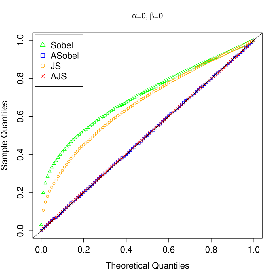
(a) Q-Q plots of p-values under $H_{00}$.

(b) Q-Q plots of p-values under $H_{01}$.

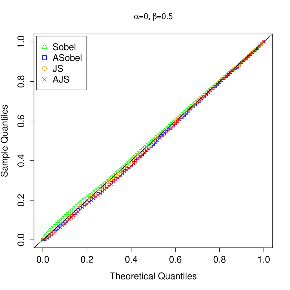
(c) Q-Q plots of p-values under $H_{10}$.

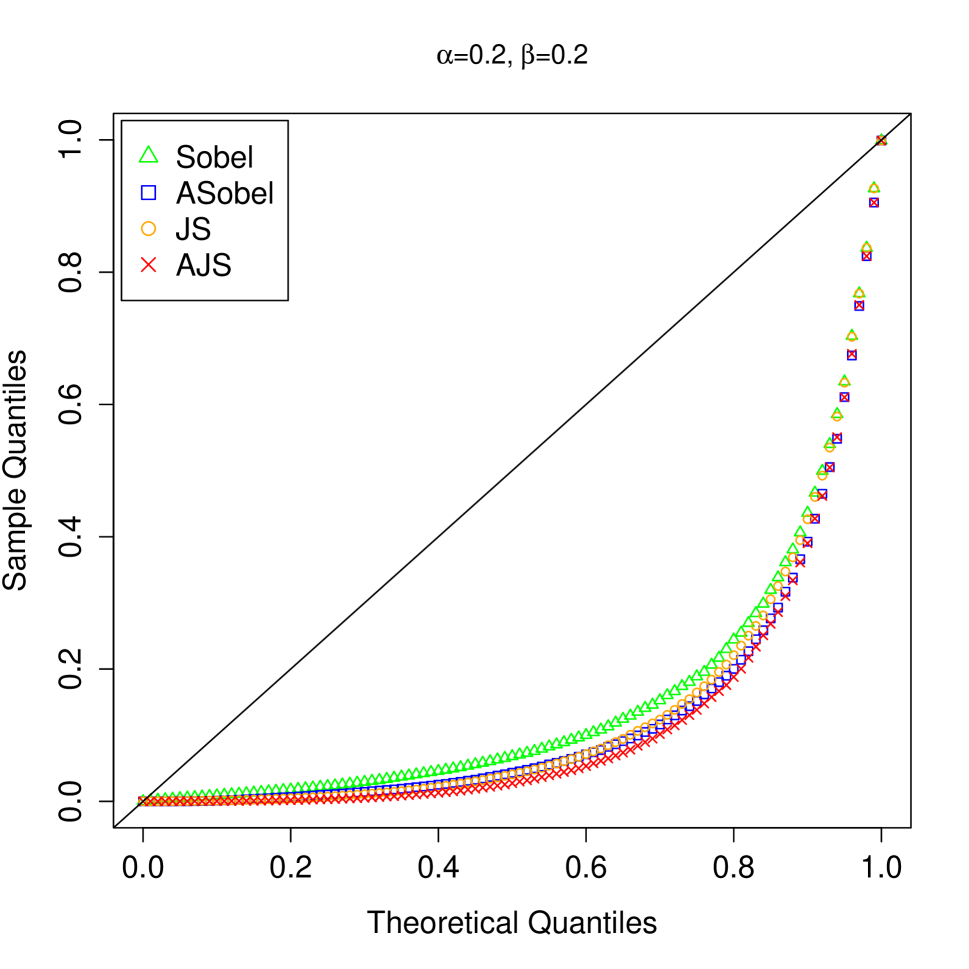
(d) Q-Q plots of p-values under $H_{A}$.

Figure S.1: Q-Q plots of p-values under logistic mediation model with $n=500$.

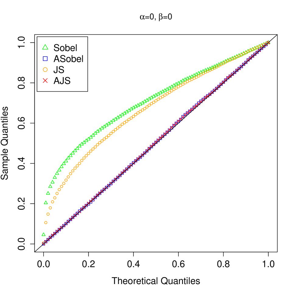
(a) Q-Q plots of p-values under $H_{00}$.

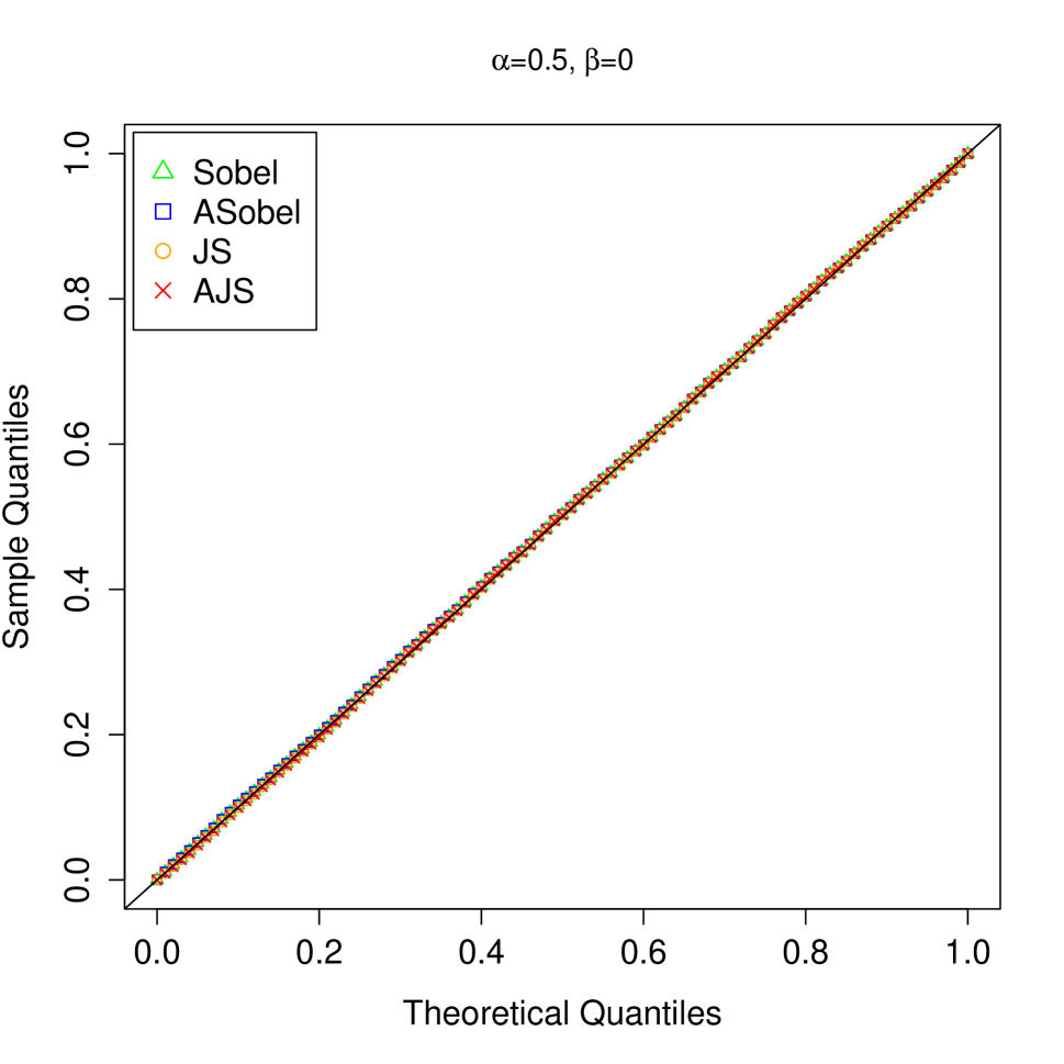
(b) Q-Q plots of p-values under $H_{01}$.

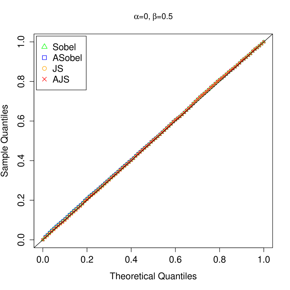
(c) Q-Q plots of p-values under $H_{10}$.

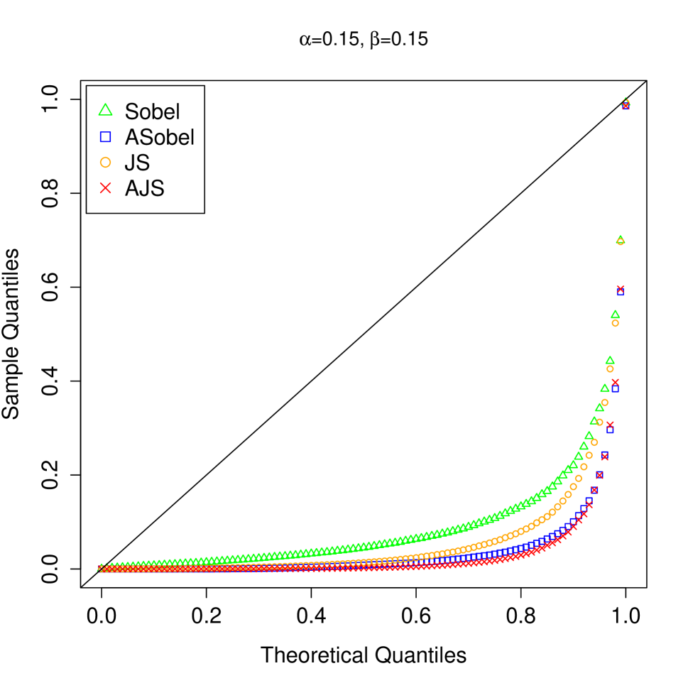
(d) Q-Q plots of p-values under $H_{A}$.

Figure S.2: Q-Q plots of p-values under Cox mediation model with $n=500$.

Table S.3: The FWER and power of multiple testing with logistic mediation model.

	Dimension		Sobel	JS	JT_Comp	DACT	AJS
$n=500$	$d=10$	FWER	0.0040	0.0084	0.2036	0.0004	0.0400
		Power	0.0509	0.1833	0.0362	0.0095	0.3095
	$d=15$	FWER	0.0022	0.0050	0.2130	0	0.0390
		Power	0.0319	0.1521	0.0392	0.0279	0.2705
	$d=20$	FWER	0.0024	0.0054	0.2310	0.0024	0.0536
		Power	0.0243	0.1317	0.0489	0.0614	0.2502
$n=1500$	$d=10$	FWER	0.0076	0.0090	0.1990	0	0.0232
		Power	0.6040	0.6988	0.2276	0.0022	0.7238
	$d=15$	FWER	0.0042	0.0064	0.2152	0	0.0324
		Power	0.5477	0.6638	0.2492	0.0184	0.6915
	$d=20$	FWER	0.0026	0.0042	0.2382	0	0.0358
		Power	0.5075	0.6398	0.2846	0.0907	0.6696

Table S.4: The FWER and power of multiple testing with Cox mediation model.

	Dimension		Sobel	JS	JT_Comp	DACT	AJS
$n=500$	$d=10$	FWER	0.0074	0.0126	0.1630	0	0.0286
		Power	0.4138	0.5503	0.4234	0.0116	0.6609
	$d=15$	FWER	0.0032	0.0056	0.1548	0	0.0320
		Power	0.3842	0.5164	0.4219	0.0862	0.6225
	$d=20$	FWER	0.0038	0.0054	0.1794	0.0004	0.0384
		Power	0.3676	0.4967	0.4325	0.2216	0.6000
$n=1500$	$d=10$	FWER	0.0098	0.0104	0.1618	0	0.0254
		Power	0.8475	0.8998	0.6243	0.0006	0.9230
	$d=15$	FWER	0.0050	0.0056	0.1678	0	0.0344
		Power	0.8131	0.8820	0.6209	0.1289	0.9082
	$d=20$	FWER	0.0052	0.0058	0.1954	0	0.0364
		Power	0.7922	0.8683	0.6462	0.3465	0.8944

Table S.5: The coverage probability and length of 95% confidence interval with logistic mediation model^‡.

			CP				LCI
	$(\alpha_{k},\beta_{k})$		Sobel		ASobel		Sobel		ASobel
$n=500$	(0, 0)		1		0.9532		0.02763		0.01384
	(0.35, 0)		0.9544		0.9544		0.17854		0.17854
	(0.5, 0)		0.9520		0.9520		0.25399		0.25399
	(0, 0.55)		0.9738		0.9038		0.10265		0.09341
	(0, 0.75)		0.9620		0.9580		0.13761		0.13700
	(0.25, 0.25)		0.9484		0.9398		0.13730		0.13622
	(0.35, 0.35)		0.9528		0.9528		0.18783		0.18783
$n=1500$	(0, 0)		1		0.9588		0.00893		0.00447
	(0.35, 0)		0.9480		0.9480		0.10026		0.10026
	(0.5, 0)		0.9500		0.9500		0.14308		0.14308
	(0, 0.55)		0.9612		0.9580		0.05695		0.05672
	(0, 0.75)		0.9582		0.9582		0.07716		0.07716
	(0.25, 0.25)		0.9484		0.9484		0.07706		0.07706
	(0.35, 0.35)		0.9540		0.9540		0.10567		0.10567

${\ddagger}$ “CP” denotes the empirical coverage probability; “LCI” denotes the length of 95% confidence interval; “Sobel” denotes the ${\rm CI_{Sobel}}$; “ASobel” denotes the proposed ${\rm CI_{ASobel}}$.

Table S.6: The coverage probability and length of 95% confidence interval with Cox mediation model^‡.

			CP				LCI
	$(\alpha_{k},\beta_{k})$		Sobel		ASobel		Sobel		ASobel
$n=500$	(0, 0)		1		0.9554		0.01238		0.00620
	(0.35, 0)		0.9520		0.9520		0.08082		0.08082
	(0.5, 0)		0.9548		0.9548		0.11541		0.11541
	(0, 0.5)		0.9588		0.9588		0.08979		0.08979
	(0, 0.45)		0.9570		0.9570		0.08050		0.08050
	(0.25, 0.25)		0.9404		0.9400		0.07435		0.07420
	(0.35, 0.35)		0.9486		0.9486		0.10231		0.10231
$n=1500$	(0, 0)		1		0.9480		0.00413		0.00206
	(0.35, 0)		0.9514		0.9514		0.04561		0.04561
	(0.5, 0)		0.9448		0.9448		0.06516		0.06516
	(0, 0.5)		0.9500		0.9500		0.05104		0.05104
	(0, 0.45)		0.9550		0.9550		0.04588		0.04588
	(0.25, 0.25)		0.9414		0.9414		0.04184		0.04184
	(0.35, 0.35)		0.9510		0.9510		0.05792		0.05792

${\ddagger}$ “CP” denotes the empirical coverage probability; “LCI” denotes the length of 95% confidence interval; “Sobel” denotes the ${\rm CI_{Sobel}}$; “ASobel” denotes the proposed ${\rm CI_{ASobel}}$.

References

- Baron and Kenny (1986) Baron, R. M. and D. A. Kenny (1986). The moderator–mediator variable distinction in social psychological research: Conceptual, strategic, and statistical considerations. Journal of Personality and Social Psychology 51(6), 1173–1182.
- Cox (1972) Cox, D. R. (1972). Regression models and life-tables (with discussions). Journal of the Royal Statistical Society, Series B 34, 187–220.
- Dai et al. (2022) Dai, J. Y., J. L. Stanford, and M. LeBlanc (2022). A multiple-testing procedure for high-dimensional mediation hypotheses. Journal of the American Statistical Association 117, 198–213.
- Huang (2019) Huang, Y.-T. (2019). Genome-wide analyses of sparse mediation effects under composite null hypotheses. The Annals of Applied Statistics 13, 60–84.
- Huang and Yang (2017) Huang, Y.-T. and H.-I. Yang (2017, May). Causal mediation analysis of survival outcome with multiple mediators. Epidemiology 28(3), 370–378.
- Liu et al. (2022) Liu, Z., J. Shen, R. Barfield, J. Schwartz, A. A. Baccarelli, and X. Lin (2022). Large-scale hypothesis testing for causal mediation effects with applications in genome-wide epigenetic studies. Journal of the American Statistical Association 117, 67–81.
- Luo et al. (2020) Luo, C., B. Fa, Y. Yan, Y. Wang, Y. Zhou, Y. Zhang, and Z. Yu (2020, April). High-dimensional mediation analysis in survival models. PLOS Computational Biology 16(4), e1007768.
- MacKinnon (2008) MacKinnon, D. P. (2008). Introduction to Statistical Mediation Analysis. New York: Taylor and Francis Group.
- MacKinnon et al. (2007) MacKinnon, D. P., A. J. Fairchild, and M. S. Fritz (2007). Mediation analysis. Annual Review of Psychology 58, 593–614.
- MacKinnon et al. (2002) MacKinnon, D. P., C. M. Lockwood, J. M. Hoffman, S. G. West, and V. Sheets (2002). A comparison of methods to test mediation and other intervening variable effects. Psychological Methods 7, 83–104.
- Mackinnon et al. (2004) Mackinnon, D. P., C. M. Lockwood, and J. Williams (2004). Confidence limits for the indirect effect: Distribution of the product and resampling methods. Multivariate Behavioral Research 39, 99–128.
- Perera et al. (2022) Perera, C., H. Zhang, Y. Zheng, L. Hou, A. Qu, C. Zheng, K. Xie, and L. Liu (2022). HIMA2: high-dimensional mediation analysis and its application in epigenome-wide dna methylation data. BMC Bioinformatics 23, 296.
- Preacher (2015) Preacher, K. J. (2015). Advances in mediation analysis: A survey and synthesis of new developments. Annual Review of Psychology 66, 825–852.
- Sampson et al. (2018) Sampson, J. N., S. M. Boca, S. C. Moore, and R. Heller (2018). FWER and FDR control when testing multiple mediators. Bioinformatics 34, 2418–2424.
- Shen et al. (2014) Shen, E., C.-P. Chou, M. A. Pentz, and K. Berhane (2014). Quantile mediation models: A comparison of methods for assessing mediation across the outcome distribution. Multivariate Behavioral Research 49, 471–485.
- Sobel (1982) Sobel, M. E. (1982). Asymptotic confidence intervals for indirect effects in structural equation models. Sociological Methodology 13, 290–312.
- Sohn and Li (2019) Sohn, M. B. and H. Li (2019, March). Compositional mediation analysis for microbiome studies. The Annals of Applied Statistics 13(1), 661–681.
- Sohn et al. (2022) Sohn, M. B., J. Lu, and H. Li (2022). A compositional mediation model for a binary outcome: Application to microbiome studies. Bioinformatics 38, 16–21.
- Sun et al. (2021) Sun, R., X. Zhou, and X. Song (2021). Bayesian causal mediation analysis with latent mediators and survival outcome. Structural Equation Modeling 28, 778–790.
- Tian et al. (2022) Tian, P., M. Yao, T. Huang, and Z. Liu (2022). CoxMKF: a knockoff filter for high-dimensional mediation analysis with a survival outcome in epigenetic studies. Bioinformatics 38, 5229–5235.
- VanderWeele (2011) VanderWeele, T. J. (2011, July). Causal mediation analysis with survival data. Epidemiology 22(4), 582–585.
- VanderWeele and Tchetgen (2017) VanderWeele, T. J. and E. J. T. Tchetgen (2017). Mediation analysis with time varying exposures and mediators. Journal of the Royal Statistical Society: Series B (Statistical Methodology) 79, 917–938.
- Vanderweele and Vansteelandt (2009) Vanderweele, T. J. and S. Vansteelandt (2009). Conceptual issues concerning mediation, interventions and composition. Statistics and Its Interface 2, 457–468.
- VanderWeele and Vansteelandt (2010) VanderWeele, T. J. and S. Vansteelandt (2010). Odds ratios for mediation analysis for a dichotomous outcome. American Journal of Epidemiology 172, 1339–1348.
- Wang et al. (2020) Wang, C., J. Hu, M. J. Blaser, and H. Li (2020, July). Estimating and testing the microbial causal mediation effect with high-dimensional and compositional microbiome data. Bioinformatics 36, 347–355.
- Wang and Zhang (2011) Wang, L. and Z. Zhang (2011). Estimating and testing mediation effects with censored data. Structural Equation Modeling 18, 18–34.
- Yu and Li (2017) Yu, Q. and B. Li (2017). mma: an R package for mediation analysis with multiple mediators. Journal of Open Research Software 5, p.11.
- Yue and Hu (2022) Yue, Y. and Y.-J. Hu (2022). A new approach to testing mediation of the microbiome at both the community and individual taxon levels. Bioinformatics 38, 3173–3180.
- Zhang et al. (2021) Zhang, H., J. Chen, Z. Li, and L. Liu (2021). Testing for mediation effect with application to human microbiome data. Statistics in Biosciences 13, 313–328.
- Zhang et al. (2022) Zhang, H., L. Hou, and L. Liu (2022). A review of high-dimensional mediation analyses in DNA methylation studies. In Guan, Weihua (Ed.), Epigenome-Wide Association Studies: Methods and Protocols 2432.
- Zhang et al. (2021) Zhang, H., Y. Zheng, L. Hou, C. Zheng, and L. Liu (2021). Mediation analysis for survival data with high-dimensional mediators. Bioinformatics 37, 3815–3821.
- Zhang et al. (2016) Zhang, H., Y. Zheng, Z. Zhang, T. Gao, B. Joyce, G. Yoon, W. Zhang, J. Schwartz, A. Just, E. Colicino, P. Vokonas, L. Zhao, J. Lv, A. Baccarelli, L. Hou, and L. Liu (2016). Estimating and testing high-dimensional mediation effects in epigenetic studies. Bioinformatics 32(20), 3150–3154.
- Zhang and Wang (2013) Zhang, Z. and L. Wang (2013). Methods for mediation analysis with missing data. Psychometrika 78, 154–184.
- Zhou (2022) Zhou, X. (2022). Semiparametric estimation for causal mediation analysis with multiple causally ordered mediators. Journal of the Royal Statistical Society: Series B (Statistical Methodology) 84, 794–821.
Supplementary Materials for