$\mathrm{SE}(3)$ diffusion model with application to protein backbone generation

Abstract

The design of novel protein structures remains a challenge in protein engineering for applications across biomedicine and chemistry. In this line of work, a diffusion model over rigid bodies in 3D (referred to as frames) has shown success in generating novel, functional protein backbones that have not been observed in nature. However, there exists no principled methodological framework for diffusion on $\mathrm{SE}(3)$, the space of orientation preserving rigid motions in $\mathbb{R}^{3}$, that operates on frames and confers the group invariance. We address these shortcomings by developing theoretical foundations of $\mathrm{SE}(3)$ invariant diffusion models on multiple frames followed by a novel framework, $\mathrm{FrameDiff}$, for learning the $\mathrm{SE}(3)$ equivariant score over multiple frames. We apply $\mathrm{FrameDiff}$ on monomer backbone generation and find it can generate designable monomers up to 500 amino acids without relying on a pretrained protein structure prediction network that has been integral to previous methods. We find our samples are capable of generalizing beyond any known protein structure. Code: https://github.com/jasonkyuyim/se3_diffusion

1 Introduction

Figure 1: Method overview. (A) Backbone parameterization with frames. Each residue along the protein chain shares the same structure of backbone atoms due to the fixed bonds between each atom. Performing the GramSchmidt operation on vectors $v_{1},v_{2}$ results in rotation matrix $r$ that parameterizes the $\texttt{N}-\texttt{C}_{\alpha}-\texttt{C}$ placements with respect to the frame translation, $x$, set to the $\texttt{C}_{\alpha}$ coordinates. An additional torsion angle, $\psi$, is required to determine the placement of the oxygen atom, O. (B) Inference is performed by sampling $N$ frames initialized from the reference distribution over rotations and translations. Then a time-reversed $\mathrm{SE}(3)$ diffusion is run from $t=\mathrm{T}_{\mathrm{F}}$ to $t=0$ at which point the $\psi$ angle is predicted. The final frames and $\psi$ angles are used to construct the protein backbone atoms.

The ability to engineer novel proteins holds promise in developing bio-therapeutics towards global health challenges such as SARS-COV-2 (Arunachalam et al., 2021) and cancer (Quijano-Rubio et al., 2020). Unfortunately, efforts to engineer proteins have required substantial domain knowledge and laborious experimental testing. To this end, protein engineering has benefited from advancements in deep learning by automating knowledge acquisition from data and improving efficiency in designing proteins (Ding et al., 2022).

Generating a novel protein satisfying specified structural or functional properties is the task of de novo protein design (Huang et al., 2016). In this work, we focus on generating protein backbones. A protein backbone consists of $N$ residues, each with four heavy atoms rigidly connected via covalent bonds, $\texttt{N}-\texttt{C}_{\alpha}-\texttt{C}-\texttt{O}$. Computationally designing novel backbones is technically challenging due to the coupling of structure and sequence: atoms that comprise protein structure must adhere to physical and chemical constraints while being “designable” in the sense that there exists a sequence of amino acids which folds to that structure. We approach this problem with diffusion generative modeling which has shown promise in recent work (see Sec. 6).

A main technical challenge is to combine expressive geometric deep learning methods that operate on protein structures with diffusion generative modeling. Because the $\texttt{N}-\texttt{C}_{\alpha}-\texttt{C}$ atoms for each residue may be described accurately as a frame (Fig. 1A), many successful computational methods for both protein structure prediction (Jumper et al., 2021) and design (Watson et al., 2022) represent backbone structures by an element of the Lie group $\mathrm{SE}(3)^{N}.$ Moreover, since the biochemical function of proteins is imparted by the relative geometries of the atoms (and so is invariant to rigid transformations) these methods typically utilize $\mathrm{SE}(3)$ equivariant neural networks. While De Bortoli et al. (2022); Huang et al. (2022) have extended diffusion modeling to Riemannian manifolds (such as $\mathrm{SE}(3)$), these works do not readily provide tractable training procedures or accommodate inclusion of geometric invariances.

Modeling $\mathrm{SE}(3)^{N}$ poses theoretical challenges and current deep learning methods have outpaced theoretical foundations. Watson et al. (2022) demonstrated a diffusion model (RFdiffusion) to generate novel protein-binders with high, experimental-verified affinities, but relied on a heuristic denoising loss and required pretraining on protein structure prediction. Our goal is to bridge this theory-practice gap and develop a principled method without pretraining.

The contribution of this work is on the theory and methodology of $\mathrm{SE}(3)$ diffusion models with applications to protein backbone generation. First, we construct a diffusion process on $\mathrm{SE}(3)^{N}$. In Sec. 3, we characterize the distribution of the Brownian motion on compact Lie groups (with a focus on $\mathrm{SO}(3)$) in a form amenable for denoising score matching (DSM) training and define a forward process on $\mathrm{SE}(3)^{N}$ that allows for separation of translations and rotations. We show that an $\mathrm{SE}(3)$ invariant process on $\mathrm{SE}(3)^{N}$ can only be made translation invariant by keeping the diffusion process centered at the origin since no $\mathbb{R}^{3}$ invariant probability measure exists. Second, we implement our theory as a $\mathrm{SE}(3)$ invariant diffusion model on $\mathrm{SE}(3)^{N}$ for protein backbones. We refer to our method as $\mathrm{FrameDiff}$ and describe it in Sec. 4. Empirically, we find through experiments in Sec. 5 that $\mathrm{FrameDiff}$ can generate designable, diverse, and novel protein monomers up to length 500. Compared to other methods, $\mathrm{FrameDiff}$ achieves in-silico designability success rates that are second only to RFdiffusion, a pretrained model with 4-fold more parameters. Our contributions will enable further advancements in $\mathrm{SE}(3)$ diffusion methodology that underlies RFdiffusion and $\mathrm{FrameDiff}$ for proteins as well as other domains such as robotics where $\mathrm{SE}(3)$ and other Lie groups are used.

2 Preliminaries and Notation

Backbone parameterization.

We adopt the backbone frame parameterization used in AlphaFold2 (AF2) (Jumper et al., 2021). Here, an $N$ residue backbone is parameterized by a collection of $N$ orientation preserving rigid transformations, or frames, that map from fixed coordinates $\texttt{N}^{\star},\texttt{C}_{\alpha}^{\star},\texttt{C}^{\star},\texttt{O}^{*}\in\mathbb{R}^{3}$ centered at $\texttt{C}_{\alpha}^{\star}=(0,0,0)$ (Fig. 1A). Each fixed coordinate assumes chemically idealized bond angles and lengths measured experimentally (Engh & Huber, 2012). For each residue indexed by $n$, the backbone main atom coordinates are given by

$$[\texttt{N}_{n},\texttt{C}_{n},(\texttt{C}_{\alpha})_{n}] =T_{n}\cdot[\texttt{N}^{\star},\texttt{C}^{\star},\texttt{C}_{\alpha}^{\star}],$$ (1)

where $T_{n}$ is a member of the special Euclidean group $\mathrm{SE}(3)$, the set of orientation preserving rigid transformations in Euclidean space. Each $T_{n}$ may be decomposed into two components $T_{n}=(r_{n},x_{n})$ where $r_{n}\in\mathrm{SO}(3)$ is a $3\times 3$ rotation matrix and $x_{n}\in\mathbb{R}^{3}$ represents a translation; for a coordinate $v\in\mathbb{R}^{3},$ $T_{n}\cdot v=r_{n}v+x_{n}$ denotes the action of $T_{n}$ on $v.$ Together, we collectively denote all $N$ frames as $\mathbf{T}=[T_{1},\dots,T_{N}]\in\mathrm{SE}(3)^{N}.$ With an additional torsion angle $\psi$, we may construct the backbone oxygen by rotating $\texttt{O}^{\star}$ around the bond between $\texttt{C}_{\alpha}$ and C. Sec. I.1 provides additional details on this mapping and idealized coordinates.

Diffusion modeling on manifolds.

To capture a distribution over backbones in $\mathrm{SE}(3)^{N}$ we build on the Riemannian score based generative modeling approach of De Bortoli et al. (2022). We briefly review this approach. The goal of Riemannian score based generative modeling is to sample from a distribution $\mathbf{X}^{(0)}\sim p_{0}$ supported on a Riemannian manifold $\mathcal{M}$ by reversing a stochastic process that transforms data into noise. One first constructs an $\mathcal{M}$-valued forward process $(\mathbf{X}^{(t)})_{t\geq 0}$ that evolves from $p_{0}$ towards an invariant density $p_{\mathrm{inv}}(x)\propto\mathrm{e}^{-U(x)}$ following

$$\textstyle{\mathrm{d}\mathbf{X}^{(t)}={-\tfrac{1}{2}\nabla U(\mathbf{X}^{(t)})}\mathrm{d}t+\mathrm{d}\mathbf{B}_{\mathcal{M}}^{(t)},\qquad\mathbf{X}^{(0)}\sim p_{0},}$$ (2)

where $\mathbf{B}_{\mathcal{M}}^{(t)}$ is the Brownian motion on $\mathcal{M}.$ The time-reversal of this process is given by the following proposition.

Proposition 2.1 (Time-reversal, De Bortoli et al. (2022)).

Let $\mathrm{T}_{\mathrm{F}}>0$ and $\overleftarrow{\mathbf{X}}^{(t)}$ given by $\overleftarrow{\mathbf{X}}^{(0)}\stackrel{{\scriptstyle d}}{{=}}\mathbf{X}^{(\mathrm{T}_{\mathrm{F}})}$ and

$$\textstyle{\mathrm{d}\overleftarrow{\mathbf{X}}^{(t)}=\{\tfrac{1}{2}\nabla U(\overleftarrow{\mathbf{X}}^{(t)})+\nabla\log p_{\mathrm{T}_{\mathrm{F}}-t}(\overleftarrow{\mathbf{X}}^{(t)})\}\mathrm{d}t+\mathrm{d}\mathbf{B}_{\mathcal{M}}^{(t)},}$$ (3)

where $p_{t}$ is the density of $\mathbf{X}^{(t)}$. Then under mild assumptions on $\mathcal{M}$ and $p_{0}$ we have that $\overleftarrow{\mathbf{X}}^{(t)}\stackrel{{\scriptstyle d}}{{=}}\mathbf{X}^{(\mathrm{T}_{\mathrm{F}}-t)}$.

Diffusion modeling in Euclidean space is a special case of Prop. 2.1. However, generative modeling using this reversal beyond the Euclidean setting requires additional mathematical machinery, which we now review.

Riemannian gradients and Brownian motions. In the above, $\nabla U(x)$ and $\nabla\log p_{t}(x)$ are Riemannian gradients taking values in $\mathrm{Tan}_{x}\mathcal{M},$ the tangent space of $\mathcal{M}$ at $x$, and depend implicitly on the choice of an inner product on $\mathrm{Tan}_{x}\mathcal{M}$, denoted by $\langle\cdot,\cdot\rangle_{\mathcal{M}}.$ Similarly, the Brownian motion relies on $\langle\cdot,\cdot\rangle_{\mathcal{M}}$ through the Laplace–Beltrami operator, $\Delta_{\mathcal{M}},$ which dictates its density through the Fokker-Planck equation in the absence of drift; if $\pi_{t}$ is the density of the $\mathbf{B}_{\mathcal{M}}^{(t)}$ then ${\partial_{t}}\pi_{t}=\frac{1}{2}\Delta_{\mathcal{M}}\pi_{t}$. We refer the reader to Lee (2013) and Hsu (2002) for background on differential geometry and stochastic analysis on manifolds.

Denoising score matching. The quantity $\nabla\log p_{t}$ is called the Stein score and is unavailable in practice. It is approximated with a score network $s_{\theta}(t,\cdot)$ trained by minimizing a denoising score matching (DSM) loss

$$\textstyle{\mathcal{L}(\theta)=\mathbb{E}[\lambda_{t}\|\nabla\log p_{t|0}(\mathbf{X}^{(t)}|\mathbf{X}^{(0)})-s_{\theta}(t,\mathbf{X}^{(t)})\|^{2}],}$$ (4)

where $p_{t|0}$ is the density of $\mathbf{X}^{(t)}$ given $\mathbf{X}^{(0)}$, $\lambda_{t}>0$ a weight, and the expectation is taken over $t\sim\mathcal{U}([0,\mathrm{T}_{\mathrm{F}}])$ and $(\mathbf{X}^{(0)},\mathbf{X}^{(t)})$. For an arbitrarily flexible network, the minimizer $\theta^{\star}=\mathrm{argmin}_{\theta}\mathcal{L}(\theta)$ satisfies $s_{\theta^{\star}}(t,\cdot)=\nabla\log p_{t}$.

Lie groups are Riemannian manifolds with an additional group structure, i.e. there exists an operator $*:G\times G\rightarrow G$ such that $(G,*)$ is a group and $*$ as well as its inverse are smooth. We define the left action as $L_{g}(h)=g*h$ for any $g,h\in G$ and its differential is denoted by $\mathrm{d}L_{g}(h):\mathrm{Tan}_{g}G\rightarrow\mathrm{Tan}_{g*h}G$. $\mathrm{SO}(3)$, $\mathrm{SE}(3)$ and $\mathbb{R}^{3}$ are all Lie groups. For any group $G$, we denote $\mathfrak{g}$ its Lie algebra. We refer to Sola et al. (2018) for an introduction to Lie groups.

Additional notation. Superscripts with parentheses are reserved for time, i.e. $x^{(t)}$. Uppercase is used to denotes random variables, e.g. $X\sim p$, and lower case is used for deterministic variables. Bold denotes concatenated versions of variables, e.g. $\mathbf{x}=(x_{1},\dots,x_{N})$ or processes $(\mathbf{X}^{(t)})_{t\in\left[0,\mathrm{T}_{\mathrm{F}}\right]}$.

3 Diffusion models on $\mathrm{SE}(3)$

Parameterizing flexible distributions over protein backbones, leveraging the Riemannian diffusion method of Sec. 2 to $\mathrm{SE}(3)^{N}$, requires several ingredients. First, in Sec. 3.1 we develop a forward diffusion process on $\mathrm{SE}(3)$, then Sec. 3.2 derives DSM training on compact Lie groups, using $\mathrm{SO}(3)$ as the motivating example. At this point, a diffusion model on $\mathrm{SE}(3)^{N}$ is defined. Next, because incorporating invariances can improve data efficiency and generalization (e.g. Elesedy & Zaidi, 2021) we desire $\mathrm{SE}(3)$ invariance where the $\mathrm{SE}(3)^{N}$ data distribution is invariant to global rotations and translations. Sec. 3.3 will show this is not possible without centering the process at the origin and having a $\mathrm{SO}(3)$-equivariant neural network.

3.1 Forward diffusion on $\mathrm{SE}(3)$

In contrast to Euclidean space and compact manifolds, no canonical forward diffusion on $\mathrm{SE}(3)^{N}$ exists, and we must define one. This entails (a) choosing an inner product on $\mathrm{SE}(3)$ to define a Brownian motion and (b) choosing a reference measure for the forward diffusion.

We begin with the inner product, which we derive from the canonical inner products for $\mathrm{SO}(3)$ and $\mathbb{R}^{3}$ which we recall below–see Carmo (1992). For $u,v\in\mathfrak{so}(3)$ and $x,y\in\mathbb{R}^{3}$

$$\textstyle{\langle u,v\rangle_{\mathrm{SO}(3)}=\mathrm{Tr}(uv^{\top})/2\mathrm{\ and\ }\langle x,y\rangle_{\mathbb{R}^{3}}=\sum_{i=1}^{3}x_{i}y_{i},}$$ (5)

In the next proposition, we show that, under an appropriate choice of inner product, $\mathrm{SE}(3)$ can be identified with $\mathrm{SO}(3)\times\mathbb{R}^{3}$ from a Riemannian point of view, thereby providing a Laplace-Beltrami operator and a well-defined Brownian motion.

Proposition 3.1 (Metric on $\mathrm{SE}(3)$).

For any $T\in\mathrm{SE}(3)$ and $(a,x),(a^{\prime},x^{\prime})\in\mathrm{Tan}_{T}\mathrm{SE}(3)$ we define $\langle(a,x),(a^{\prime},x^{\prime})\rangle_{\mathrm{SE}(3)}=\langle a,a^{\prime}\rangle_{\mathrm{SO}(3)}+\langle x,x^{\prime}\rangle_{\mathbb{R}^{3}}.$ We have:

1. for any $f\in\mathrm{C}^{\infty}(\mathrm{SE}(3))$ and $T=(r,x)\in\mathrm{SE}(3)$, $\nabla_{T}f(T)=[\nabla_{r}f(r,x),\nabla_{x}f(r,x)]$,

2. for any $f\in\mathrm{C}^{\infty}(\mathrm{SE}(3))$ and $T=(r,x)\in\mathrm{SE}(3)$, $\Delta_{\mathrm{SE}(3)}f(T)=\Delta_{\mathrm{SO}(3)}f(r,x)+\Delta_{\mathbb{R}^{3}}f(r,x)$,

3. for any $t>0$, $\mathbf{B}_{\mathrm{SE}(3)}^{(t)}=[\mathbf{B}_{\mathrm{SO}(3)}^{(t)},\mathbf{B}_{\mathbb{R}^{3}}^{(t)}]$ with independent $\mathbf{B}_{\mathrm{SO}(3)}^{(t)}$ and $\mathbf{B}_{\mathbb{R}^{3}}^{(t)}.$

Other choices of metric for $\mathrm{SE}(3)$ are possible, leading to different definitions of the exponential and Brownian motion. Our choice has the advantage of simplicity and allows to treat $\mathrm{SO}(3)$ and $\mathbb{R}^{3}$ forward processes independently (conditionally on $\mathbf{T}^{(0)}$). For the invariant density of $T=(r,x)$, we choose $p_{\mathrm{inv}}^{\mathrm{SE}(3)}(T)\propto\mathcal{U}^{\mathrm{SO}(3)}(r)~{}\mathcal{N}(x;0,\operatorname{Id}_{3})$. The associated forward process $(\mathbf{T}^{(t)})_{t\geq 0}=(\mathbf{R}^{(t)},\mathbf{X}^{(t)})_{t\geq 0}$ is given according to (2) and Prop. 3.1 by

$$\mathrm{d}\mathbf{T}^{(t)}=[0,-\tfrac{1}{2}\mathbf{X}^{(t)}]\mathrm{d}t+[\mathrm{d}\mathbf{B}_{\mathrm{SO}(3)}^{(t)},\mathrm{d}\mathbf{B}_{\mathbb{R}^{3}}^{(t)}].$$ (6)

3.2 Denoising score matching on $\mathrm{SE}(3)$

As a consequence of Prop. 3.1 and the independence of the rotational and translational components of the forward process, we have $\nabla_{\mathbf{T}^{(t)}}\log p_{t|0}(\mathbf{T}^{(t)}|\mathbf{T}^{(0)})=[\nabla_{\mathbf{R}^{(t)}}\log p_{t|0}(\mathbf{R}^{(t)}|\mathbf{R}^{(0)}),\nabla_{\mathbf{X}^{(t)}}\log p_{t|0}(\mathbf{X}^{(t)}|\mathbf{X}^{(0)})]$ and we can compute these quantities independently over the rotation and translation components.

Denoising score matching on $\mathrm{SO}(3)$. The forward process $(\mathbf{R}^{(t)})_{t\geq 0}$ is simply the Brownian motion on $\mathrm{SO}(3)$, and $p_{t|0}$ is defined by the heat kernel, see Hsu (2002). We obtain $p_{t|0}$ analytically as a series as a special case of the decomposition of the heat kernel for compact Lie groups.

Proposition 3.2 (Brownian motion on compact Lie groups).

Assume that $\mathcal{M}$ is a compact Lie group, where for any $\ell\in\mathbb{N}$ $\chi_{\ell}$ is the character associated with the irreducible unitary representation of dimension $d_{\ell}$. Then $\chi_{\ell}:\ \mathcal{M}\to\mathbb{R}$ is an eigenvector of $\Delta$ and there exists $\lambda_{\ell}\geq 0$ such that $\Delta\chi_{\ell}=-\lambda_{\ell}\chi_{\ell}$. In addition, we have for any $t>0$ and $x^{(0)},x^{(t)}\in\mathcal{M}$, $\textstyle{p_{t|0}(x^{(t)}|x^{(0)})=\sum_{\ell\in\mathbb{N}}d_{\ell}e^{-\lambda_{\ell}t/2}\chi_{\ell}((x^{(0)})^{-1}x^{(t)}).}$

Combining Prop. 3.2 and the explicit expression of irreducible characters for $\mathrm{SO}(3)$ provides an explicit expression for the density transition kernel $\mathbf{B}_{\mathrm{SO}(3)}^{(t)}.$ In Sec. E.1, we showcase another application of our method by computing the heat kernel on $\mathrm{SU}(2)$.

Proposition 3.3 (Brownian motion on $\mathrm{SO}(3)$).

For any $t>0$ and $r^{(0)},r^{(t)}\in\mathrm{SO}(3)$ we have that $p_{t|0}(r^{(t)}|r^{(0)})=\mathrm{IGSO}_{3}(r^{(t)};r^{(0)},t)$ given by $\mathrm{IGSO}_{3}(r^{(t)};r^{(0)},t)=f(\omega(r^{(0)\top}r^{(t)}),t)$, where $\omega(r)$ is the rotation angle in radians for any $r\in\mathrm{SO}(3)$—its length in the axis–angle representation— and

$$f(\omega,t)=\textstyle{\sum_{\ell\in\mathbb{N}}(2\ell+1)\mathrm{e}^{-\ell(\ell+1)t/2}\tfrac{\sin((\ell+1/2)\omega)}{\sin(\omega/2)}.}$$ (7)

Prop. 3.3 agrees with previous proposed expressions of the law of the Brownian motion (Nikolayev & Savyolov, 1970; Leach et al., 2022) up to a two-fold deceleration of time. This deceleration is crucial to the correct application of Prop. 2.1 (see Sec. E.3 for details).

Accurate values of the Brownian density (7) can easily be obtained by truncating the series. Also, although exact sampling is not available, accurate samples can be obtained by numerically inverting the cdf (Leach et al., 2022). Moreover, this density allows computation of the conditional score required by the $\mathrm{dsm}$ loss.

Proposition 3.4 (Score on $\mathrm{SO}(3)$).

For $t>0$, $r^{(0)},r^{(t)}\in\mathrm{SO}(3)$, we have

$$\nabla\log p_{t|0}(r^{(t)}\mid r^{(0)})=\tfrac{r^{(t)}}{\omega^{(t)}}\log\{r^{(0,t)}\}\frac{\partial_{\omega}f(\omega^{(t)},t)}{f(\omega^{(t)},t)},$$ (8)

with $r^{(0,t)}=r^{(0)\top}r^{(t)}$, $\omega^{(t)}=\omega(r^{(0,t)})$ and $\log$ the inverse of the exponential on $\mathrm{SO}(3),$ i.e. the matrix logarithm.

Denoising score matching on $\mathbb{R}^{3}$. The process $(\mathbf{X}^{(t)})_{t\geq 0}$ is an Ornstein–Uhlenbeck process, see (6), (also called VP-SDE (Song et al., 2021)) and converges geometrically to $\mathcal{N}(0,\operatorname{Id})$. In addition, $p_{t|0}(x^{(t)}|x^{(0)})=\mathcal{N}(x^{(t)};\mathrm{e}^{-t/2}x^{(0)},(1-\mathrm{e}^{-t})\operatorname{Id}_{3})$ and the corresponding conditional score can be computed explicitly as

$$\nabla\log p_{t|0}(x^{(t)}|x^{(0)})=(1-\mathrm{e}^{-t})^{-1}(\mathrm{e}^{-t/2}x^{(0)}-x^{(t)}).$$ (9)

3.3 $\mathrm{SE}(3)$ invariance through centered $\mathrm{SE}(3)^{N}$

In this subsection, we show how one can construct a diffusion process over $\mathrm{SE}(3)^{N}$ that is invariant to global translations and rotations. Formally, we want to design a measure $\mu$ on $\mathrm{SE}(3)^{N}$ such that for any $T_{0}\in\mathrm{SE}(3)$, and measurable $\mathsf{A}\subset\mathrm{SE}(3)^{N},\ \ \mu(\mathsf{A})=\mu(\{T_{0}\cdot\mathbf{T}\ ,\ \mathbf{T}\in\mathsf{A}\})$, where for any $\mathbf{T}=(T_{1},\cdots,T_{N})$, $T_{0}\cdot\mathbf{T}=(T_{0}T_{1},\dots,T_{0}T_{N})$. Unfortunately, there exists no probability measure on $\mathrm{SE}(3)^{N}$ which is $\mathrm{SE}(3)$ invariant since there exists no probability measure on $\mathbb{R}^{3N}$ which is $\mathbb{R}^{3}$ invariant. As a result, no output of a $\mathrm{SE}(3)^{N}$-valued diffusion model can be $\mathrm{SE}(3)$ invariant. However, we will show $\mathrm{SE}(3)$ invariance is achieved by keeping the diffusion process always centered at the origin.

From $\mathrm{SE}(3)$ to $\mathrm{SO}(3)$ invariance. We show that we can construct an invariant measure on $\mathrm{SE}(3)^{N}$ by keeping the center of mass fixed to zero, i.e. $\sum_{n=1}^{N}x_{n}=0$. Formally, this defines a subgroup of $\mathrm{SE}(3)^{N}$ denoted $\mathrm{SE}(3)^{N}_{0}$ with elements $[(r_{1},x_{1}),\dots,(r_{N},x_{N})]$, which we refer to as centered $\mathrm{SE}(3)$. Note that $\mathrm{SE}(3)^{N}_{0}$ is still a Lie group and $\mathrm{SO}(3)$ is a subgroup of $\mathrm{SE}(3)^{N}_{0}$.

Proposition 3.5 (Disintegration of measures on $\mathrm{SE}(3)^{N}$).

Under mild assumptions, for every $\mathrm{SE}(3)$-invariant measure $\mu$ on $\mathrm{SE}(3)^{N}$, there exist $\eta$ an $\mathrm{SO}(3)$-invariant probability measure on $\mathrm{SE}(3)^{N}_{0}$ and $\bar{\mu}$ proportional to the Lebesgue measure on $\mathbb{R}^{3}$ such that

$$\textstyle{\mathrm{d}\mu([(r_{1},x_{1}),...,(r_{N},x_{N})])=\mathrm{d}\bar{\mu}(\tfrac{1}{N}\sum_{i=1}^{N}x_{i})}$$ (10)

$$\textstyle{\times\mathrm{d}\eta([(r_{1},x_{1}-\tfrac{1}{N}\sum_{i=1}^{N}x_{i}),...,(r_{N},x_{N}-\tfrac{1}{N}\sum_{i=1}^{N}x_{i})]).}$$ (11)

The previous proposition is based on the disintegration of measures (Pollard, 2002). The converse is also true. In practice this means that in order to define a $\mathrm{SE}(3)$-invariant measure on $\mathrm{SE}(3)^{N}$ one needs only to define an $\mathrm{SO}(3)$-invariant measure on $\mathrm{SE}(3)^{N}_{0}$. This is the goal of the next paragraph.

Diffusion models on $\mathrm{SE}(3)^{N}_{0}$. A simple modification of the forward process (6) yields a stochastic process on $\mathrm{SE}(3)_{0}^{N}$. Indeed consider $(\mathbf{T}^{(t)})_{t\geq 0}$ on $\mathrm{SE}(3)^{N}$ given by

$$\mathrm{d}\mathbf{T}^{(t)}=[0,-\tfrac{\mathrm{1}}{2}\mathrm{P}\mathbf{X}^{(t)}]\mathrm{d}t+[\mathrm{d}\mathbf{B}^{(t)}_{\mathrm{SO}(3)^{N}},\mathrm{P}\mathrm{d}\mathbf{B}^{(t)}_{\mathbb{R}^{3N}}],$$ (12)

where $\mathrm{P}\in\mathbb{R}^{3N\times 3N}$ is the projection matrix removing the center of mass $\tfrac{1}{N}\sum_{n=1}^{N}x_{n}$. Then $(\mathbf{T}^{(t)})_{t\geq 0}=(\mathbf{R}^{(t)},\mathbf{X}^{(t)})_{t\geq 0}$ is a stochastic process on $\mathrm{SE}(3)^{N}_{0}$ with invariant measure $\mathrm{P}_{\#}(\mathcal{N}(0,\operatorname{Id})^{\otimes N})\otimes\mathcal{U}(\mathrm{SO}(3))^{\otimes N}$. We note that such ‘center of mass free’ systems have been proposed for continuous normalizing flows and discrete time diffusion models (Köhler et al., 2020; Xu et al., 2022). An application of Props. 2.1 and 3.1 shows that the backward process $(\overleftarrow{\mathbf{T}}^{(t)})_{t\in\left[0,\mathrm{T}_{\mathrm{F}}\right]}=([\overleftarrow{\mathbf{R}}^{(t)},\overleftarrow{\mathbf{X}}^{(t)}])_{t\in\left[0,\mathrm{T}_{\mathrm{F}}\right]}$ is given by

$$\mathrm{d}\overleftarrow{\mathbf{R}}^{(t)}=\nabla_{r}\log p_{\mathrm{T}_{\mathrm{F}}-t}(\overleftarrow{\mathbf{T}}^{(t)})\mathrm{d}t+\mathrm{d}\mathbf{B}^{(t)}_{\mathrm{SO}(3)^{N}},$$ (13)

$$\mathrm{d}\overleftarrow{\mathbf{X}}^{(t)}=\mathrm{P}\{\tfrac{\mathrm{1}}{2}\overleftarrow{\mathbf{X}}^{(t)}+\nabla_{x}\log p_{\mathrm{T}_{\mathrm{F}}-t}(\overleftarrow{\mathbf{T}}^{(t)})\}\mathrm{d}t+\mathrm{P}\mathrm{d}\mathbf{B}^{(t)}_{\mathbb{R}^{3N}}.$$ (14)

As in Sec. 3.2, we have $p_{t|0}((\mathbf{r}^{(t)},\mathbf{x}^{(t)})|(\mathbf{r}^{(0)},\mathbf{x}^{(0)}))=p_{t|0}(\mathbf{r}^{(t)}|\mathbf{r}^{(0)})p_{t|0}(\mathbf{x}^{(t)}|\mathbf{x}^{(0)})$, where these densities additionally factorizes along each of the residues. In Sec. J.1, we use the forward process (12) for training and the backward process (13) for sampling in Sec. J.2.

Invariance and equivariance on Lie groups. Finally, we want the output of the backward process, i.e. the distribution of $(\mathbf{R}^{(t)},\mathbf{X}^{(t)})$ given by (13) to be $\mathrm{SO}(3)$-invariant so that the associated measure on $\mathrm{SE}(3)^{N}$ given by Prop. 3.5 is $\mathrm{SE}(3)$-invariant. To do so we use the following result.

Proposition 3.6 ($G$-invariance and SDEs).

Let $G$ be a Lie group and $H$ a subgroup of $G$. If (a) $\mathbf{X}^{(0)}\sim p_{0}$ for an $H$ invariant distribution $p_{0}$ and (b) $\mathrm{d}\mathbf{X}^{(t)}=b(t,\mathbf{X}^{(t)})\mathrm{d}t+\Sigma^{1/2}\mathrm{d}\mathbf{B}^{(t)}$ for bounded, $H$-equivariant coefficients $b$ and $\Sigma$ satisfying $b\circ L_{h}=\mathrm{d}L_{h}(b)$ and $\Sigma\mathrm{d}L_{h}(\cdot)=\mathrm{d}L_{h}(\Sigma\cdot),$ and where $\mathbf{B}^{(t)}$ is a Brownian motion associated with a left-invariant metric. Then for every $t\geq 0$

1. the distribution $p_{t}$ of $\mathbf{X}^{(t)}$ is $H$-invariant, and

2. its score $\nabla_{\mathbf{X}^{(t)}}\log p_{t}(\mathbf{X}^{(t)})$ is $H$-equivariant.

The proof can be extended to non-bounded coefficients under appropriate assumption on the growth of $b$. As a consequence of Prop. 3.6 we obtain the announced invariance.

Corollary 3.7.

Suppose $\{\mathbf{T}^{(0)}\}_{t\geq 0}$ has $\mathrm{SO}(3)$ invariant initial distribution $p_{0}$ and evolves according to Eq. 12. Then for every $t\in(0,\mathrm{T}_{\mathrm{F}}),\ \nabla\log p_{\mathrm{T}_{\mathrm{F}}-t}(\overleftarrow{\mathbf{T}}^{(t)})$ is $\mathrm{SO}(3)$ equivariant, and the distribution of $(\overleftarrow{\mathbf{R}}^{(t)},\overleftarrow{\mathbf{X}}^{(t)})$ implied by Eq. 13 is $\mathrm{SO}(3)$-invariant.

The significance Corollary 3.7 is two-fold. First, because the true score $\nabla\log p_{\mathrm{T}_{\mathrm{F}}-t}(\overleftarrow{\mathbf{T}}^{(t)})$ is $\mathrm{SO}(3)$-equivariant, the corollary shows that incorporating an $\mathrm{SO}(3)$-equivariance constraint into neural network approximations of the score, $[s_{\theta}^{r},s_{\theta}^{x}],$ does not limit the ability of the model to describe any $\mathrm{SO}(3)$ invariant target. Second, it shows that any such approximation $\overleftarrow{\mathbf{T}}^{(t)}$ will be $\mathrm{SO}(3)$ invariant.

Equation (3.7) is still true if $[\nabla_{r}\log p_{t},\nabla_{x}\log p_{t}]$ is replaced with $[s_{\theta}^{r},s_{\theta}^{x}]$ with $s_{\theta}^{r}$ and $s_{\theta}^{x}$ $\mathrm{SO}(3)$-equivariant neural networks, see Sec. 4.1.

4 Protein backbone diffusion model

Figure 2: Single layer of $\mathrm{FrameDiff}$. Each layer takes in the current node embedding $\mathbf{h}_{\ell}$, edge embedding $\mathbf{z}_{\ell}$, frames $\mathbf{T}_{\ell}$, and initial node embedding $\mathbf{h}_{0}$. Rectangles indicate trainable neural networks. Node embeddings are first updated using IPA with a skip connection. Before Transformer, the initial node embeddings and post-IPA embeddings are concatenated. After transformer, we include a skip connection with post-IPA embeddings. The updated node embeddings $\mathbf{h}_{\ell+1}$ are then used to update edge embeddings $\mathbf{z}_{\ell+1}$ as well as predict frame updates $\mathbf{T}_{\ell+1}$. See Sec. I.2 for in-depth architecture details.

We now describe $\mathrm{FrameDiff}$, a diffusion model for sampling protein backbones by modeling frames based on the centered $\mathrm{SE}(3)^{N}$ stochastic process in Sec. 3. In Sec. 4.1, we describe our neural network to learn the score using frame and torsion predictions. Sec. 4.2 presents a multi-objective loss involving score matching and auxiliary protein structure losses. Additional details for training and sampling are postponed to Secs. J.1 and J.2.

4.1 $\mathrm{FramePred}$: score and torsion prediction

In this section, we provide an overview of our score and torsion prediction network; technical details are given in Sec. I.2. Our neural network to learn the score is based on the structure module of AlphaFold2 (AF2) (Jumper et al., 2021), which has previously be adopted for diffusion by Anand & Achim (2022). Namely, it performs iterative updates to the frames over a series of $L$ layers using a combination of spatial and sequence based attention modules. Let $\mathbf{h}_{\ell}=[h_{\ell}^{1},\dots,h_{\ell}^{N}]\in\mathbb{R}^{N\times D_{h}}$ be the node embeddings of the $\ell$-th layer where $h_{\ell}^{n}$ is the embedding for residue $n$. $\mathbf{z}_{\ell}\in\mathbb{R}^{N\times N\times D_{z}}$ are edge embeddings with $z_{\ell}^{nm}$ being the embedding of the edge between residues $n$ and $m$.

Fig. 2 shows one single layer of our neural network. Spatial attention is performed with Invariant Point Attention (IPA) from AF2 which can attend to closer residues in coordinate space while a Transformer (Vaswani et al., 2017) allows for capturing interactions along the chain structure. We found including the Transformer greatly improved training and sample quality. As a result, the computational complexity of $\mathrm{FrameDiff}$ is quadratic in backbone length. Unlike AF2, we do not use $\mathrm{StopGradient}$ between rotation updates. The updates are $\mathrm{SE}(3)$-invariant since IPA is $\mathrm{SE}(3)$-invariant. We utilize fully connected graph structure where each residue attends to every other node. Updates to the node embeddings are propagated to the edges in $\mathrm{EdgeUpdate}$ where a standard message passing edge update is performed. $\mathrm{BackboneUpdate}$ is taken from AF2 (Algorithm 23), where a linear layer is used to predict translation and rotation updates to each frame. Feature initialization follows Trippe et al. (2023) where node embeddings are initialized with residue indices and timestep while edge embeddings additionally get relative sequence distances. Edge embeddings are additionally initialized through self-conditioning (Chen et al., 2023) with a binned pairwise distance matrix between the model’s $\texttt{C}_{\alpha}$ predictions. All coordinates are represented in nanometers.

Our model also outputs a prediction of the $\boldsymbol{\psi}$ angle for each residue, which positions the backbone oxygen atom with respect to the predicted frame. Putting it all together, our neural network with weights $\theta$ predicts the denoised frame and torsion angle,

$$(\mathbf{\hat{T}}^{(0)},\boldsymbol{\hat{\psi}})=\mathrm{FramePred}(\mathbf{T}^{(t)},t;\theta),\ \ \mathbf{\hat{T}}^{(0)}=(\mathbf{\hat{R}}^{(0)},\mathbf{\hat{X}}^{(0)}).$$ (15)

Score parameterization. We relate the $\mathrm{FrameDiff}$ prediction to a score prediction via $\nabla_{\mathbf{T}^{(t)}}\log p_{t|0}(\mathbf{T}^{(t)}\mid\mathbf{\hat{T}}^{(0)})=\{(s_{\theta}^{\mathrm{r}}(t,\mathbf{T}^{(t)})_{n},s_{\theta}^{\mathrm{x}}(t,\mathbf{T}^{(t)})_{n})\}_{n=1}^{N}$ where the predicted score is computed separately for the rotation and translation of each residue, $s_{\theta}^{\mathrm{r}}(t,\mathbf{T}^{(t)})_{n}=\nabla_{\mathbf{R}_{n}^{(t)}}\log p_{t|0}(\mathbf{R}_{n}^{(t)}|\hat{\mathbf{R}}_{n}^{(0)})$ and $s_{\theta}^{\mathrm{x}}(t,\mathbf{T}^{(t)})_{n}=\nabla_{\mathbf{X}_{n}^{(t)}}\log p_{t|0}(\mathbf{X}_{n}^{(t)}|\hat{\mathbf{X}}_{n}^{(0)}).$

4.2 Training losses

Learning the translation and rotation score amounts to minimizing the DSM loss given in (4). Following Song et al. (2021), we choose the weighting schedule for the rotation component as $\lambda^{\mathrm{r}}_{t}\!=\!1/\mathbb{E}[\|\nabla\log p_{t|0}(\mathbf{R}_{n}^{(t)}|\mathbf{R}^{(0)})\|^{2}_{\mathrm{SO}(3)}]$; with this choice, the expected loss of the trivial prediction $\hat{R}^{(0)}=R^{(t)}$ is equal to $1$ for every $t.$

For translations, we use $\lambda_{t}^{\mathrm{x}}=(1-\mathrm{e}^{-t})/\mathrm{e}^{-t/2}$ so (4) simplifies as

$$\mathcal{L}_{\mathrm{dsm}}^{\mathrm{x}} =\textstyle{\tfrac{1}{N}\sum_{n=1}^{N}\|X^{(0)}_{n}-\hat{X}^{(0)}_{n}\|^{2}}.$$ (16)

We find this choice is beneficial to avoid loss instabilities near low $t$ (see Karras et al. for more discussion) where atomic accuracy is crucial for sample quality. There is also the physical interpretation of directly predicting the $\texttt{C}_{\alpha}$ coordinates. Our $\mathrm{SE}(3)$ DSM loss is $\mathcal{L}_{\mathrm{dsm}}=\mathcal{L}_{\mathrm{dsm}}^{\mathrm{r}}+\mathcal{L}_{\mathrm{dsm}}^{\mathrm{x}}.$

Auxiliary losses. In early experiments, we found that $\mathrm{FrameDiff}$ with $\mathcal{L}_{\mathrm{dsm}}$ generated backbones with plausible coarse-grained topologies, but unrealistic fine-grained characteristics, such as chain breaks or steric clashes. To discourage these physical violations, we use two additional losses to learn torsion angle $\psi$ and directly penalize atomic errors in the last steps of generation. Let $\Omega=\{\texttt{N},\texttt{C},\texttt{C}_{\alpha},\texttt{O}\}$ be the collection of backbone atoms. The first loss is a direct MSE on the backbone (bb) positions,

$$\textstyle{\mathcal{L}_{\mathrm{bb}}=\tfrac{1}{4N}\sum_{n=1}^{N}\sum_{a\in\Omega}\|a_{n}^{(0)}-\hat{a}_{n}^{(0)}\|^{2}.}$$ (17)

Next, define $d_{ab}^{nm}=\|a^{(0)}_{n}-b^{(0)}_{m}\|$ as the true atomic distance between atoms $a,b\in\Omega$ for residue $n$ and $m$. The predicted pairwise atomic distance is $\hat{d}_{ab}^{nm}=\|\hat{a}_{n}^{(0)}-\hat{b}_{m}^{(0)}\|$. Similar in spirit to the distogram loss in AF2, the second loss is a local neighborhood loss on pairwise atomic distances,

$$\textstyle{\mathcal{L}_{2\mathrm{D}}=\frac{1}{Z}\sum_{n,m=1}^{N}\sum_{a,b\in\Omega}\mathds{1}\{d_{ab}^{nm}<0.6\}\|d_{ab}^{nm}-\hat{d}_{ab}^{nm}\|^{2},}$$ (18)

$$\textstyle{Z=(\sum_{n,m=1}^{N}\sum_{a,b\in\Omega}\mathds{1}\{d_{ab}^{nm}<0.6\})-N.}$$ (19)

where $\mathds{1}\{d_{ab}^{nm}<0.6\}$ is a indicator variable to only penalize atoms that within 0.6nm (i.e. $6$Å). We apply auxiliary losses only when $t$ is sampled near 0 ($t<\mathrm{T}_{\mathrm{F}}/4$ in our experiments) during which the fine-grained characteristics emerge. The full training loss can be written,

$$\textstyle{\mathcal{L}=\mathcal{L}_{\text{dsm}}+w\cdot\mathds{1}\{t<\frac{\mathrm{T}_{\mathrm{F}}}{4}\}(\mathcal{L}_{\mathrm{bb}}+\mathcal{L}_{2\mathrm{D}})},$$ (20)

where $w>0$ is a weight on these additional losses. We find a including a high weight ($w=0.25$ in our experiments) leads to improved sample quality with fewer steric clashes and chain breaks. Training follows standard diffusion training over the empirical data distribution $p_{0}$. A full algorithm (Alg. 3) is provided in the appendix.

Algorithm 1 $\mathrm{FrameDiff}$ sampling of protein backbones

0:  $\theta,N,\mathrm{T}_{\mathrm{F}},N_{\mathrm{steps}},\zeta,\epsilon$

1:  $\gamma=(1-\epsilon)/N_{\mathrm{steps}}$

2:  # Sample from invariant density

3:  $\mathbf{T}^{(\mathrm{T}_{\mathrm{F}})}\sim P_{\#}p_{\mathrm{inv}}^{\mathrm{SE}(3)^{N}}$

4:  for $t=\mathrm{T}_{\mathrm{F}},\mathrm{T}_{\mathrm{F}}-\gamma,\mathrm{T}_{\mathrm{F}}-2\gamma,\dots,\epsilon$ do

5:     $\hat{\mathbf{T}}^{(0)},\_=\mathrm{FramePred}(\mathbf{T}^{(t)},t;\theta)$

6:     $\{(s_{\theta,n}^{\mathrm{r}},s_{\theta,n}^{\mathrm{x}})\}_{n=1}^{N}=\nabla_{\mathbf{T}^{(t)}}\log p_{t|0}(\mathbf{T}^{(t)}\mid\hat{\mathbf{T}}^{(0)})$

7:     for $(R_{n}^{(t)},X_{n}^{(t)})=T_{1}^{(t)},\dots,T_{N}^{(t)}$ do

8:        # Translation tangent Gaussian

9:        $Z_{n}^{\mathrm{x}}\sim\mathcal{N}(0,\operatorname{Id}_{3})$

10:        $W_{n}^{\mathrm{x}}=P\gamma[\tfrac{1}{2}X_{n}^{(t)}+s^{\mathrm{x}}_{\theta,n}]+\zeta\sqrt{\gamma}Z_{n}^{\mathrm{x}}$

11:        # Remove center of mass

12:        $W_{n}^{\mathrm{x}}=PW_{n}^{\mathrm{x}}$

13:        # Rotation tangent Gaussian

14:        $Z_{n}^{\mathrm{r}}\sim\mathcal{TN}_{R_{n}^{(t)}}(0,\operatorname{Id})$

15:        # Euler–Maruyama step on tangent space

16:        $W_{n}^{\mathrm{r}}=\gamma\mathbf{s}^{\mathrm{r}}_{\theta,n}+\zeta\sqrt{\gamma}Z_{n}^{\mathrm{r}}$

17:        $T_{n}^{(t-\gamma)}=\exp_{T_{n}^{(t)}}\left\{(W_{n}^{\mathrm{r}},W_{n}^{\mathrm{x}})\right\}$

18:     end for

19:  end for

20:  Return: $\mathrm{FramePred}(\mathbf{T}^{(\epsilon)},\epsilon;\theta)$

Centering of training examples. Each training example $\mathbf{X}^{(t)}$, is centered at zero in accordance with Eq. 12. From a practical perspective, this centering leads to lower variance loss estimates than without centering. In particular, variability in the center of mass of $\mathbf{X}^{(t)}$ would lead to corresponding variability in $\mathrm{FrameDiff}$’s frame predictions as a result of the architecture’s $\mathrm{SE}(3)$ equivariance. By centering training examples, we eliminate this variability and thereby reduce the variance of $\mathcal{L}_{\mathrm{dsm}}^{\mathrm{x}}$ and of gradient estimates.

4.3 Sampling

Alg. 1 provides our sampling procedure. Following De Bortoli et al. (2022), we use an Euler–Maruyama discretization of Eq. 13 with $N_{\mathrm{steps}}$ steps implemented as a geodesic random walk. Each step involves samples $Z_{n}^{\mathrm{x}}$ and $Z_{n}^{\mathrm{r}}$ from Gaussian distributions defined in the tangent spaces of $X_{n}^{(t)}$ and $R_{n}^{(t)}$, respectively. For translations, this is simply the usual Gaussian distribution on $\mathbb{R}^{3},$ $Z_{n}^{\mathrm{x}}\sim\mathcal{N}(0,\operatorname{Id}_{3}).$ For rotations, we sample the coefficients of orthonormal basis vectors of the Lie algebra $\mathfrak{so}(3)$ and rotate them into the tangent space to generate $Z_{n}^{\mathrm{r}}\sim\mathcal{TN}_{R_{n}^{(t)}}(0,\operatorname{Id})$ as $Z_{n}^{\mathrm{r}}=R_{n}^{(t)}\sum_{i=1}^{3}\delta_{i}\mathbf{e}_{i},$ where $\delta_{i}\overset{iid}{\sim}\mathcal{N}(0,1)$ and $\mathbf{e}_{1},\mathbf{e}_{2},\mathbf{e}_{3}$ are orthonormal basis vectors (see Sec. C.2 for details).

Because we found that the backbones commonly destabilized in the final steps of sampling, we truncate sampling trajectories early, at a time $\epsilon>0.$ Following Watson et al. (2022), we explore generating from the reverse process with noise downscaled by a factor $\zeta\in\left[0,1\right].$ For simplicity of exposition, we so far have assumed that the forward diffusion involves a Brownian motion without a diffusion coefficient; in practice we set $\mathrm{T}_{\mathrm{F}}=1$ and consider different diffusion coefficients for the rotation and translation (see Sec. I.3).

5 Experiments

Figure 3: Designability, diversity, and novelty of $\mathrm{FrameDiff}$ generated backbones with $\zeta=0.1$, $N_{\mathrm{steps}}=500$, $N_{\mathrm{seq}}=100$. (A) scRMSD based on 100 backbone samples of each length 70, 100, 200, 300 for $N_{\mathrm{seq}}=8,100$ plotted in the same manner as done in RFdiffusion. (B) Scatter plot of Designability (scRMSD) vs. novelty (pdbTM) across lengths. (C) Selected samples from panel (B) of novel and highly designable samples. Left: sampled backbones from $\mathrm{FrameDiff}$. Middle: best ESMFold predictions with high confidence (pLDDT) Right: samples aligned with their closest PDB chain.

We evaluate $\mathrm{FrameDiff}$ on monomer backbone generation. We trained $\mathrm{FrameDiff}$ with $L=4$ layers on a filtered set of 20312 backbones taken from the Protein Data Bank (PDB) (Berman et al., 2000). Our model comprises 17.4 million parameters and was trained for one week on two A100 Nvidia GPUs. See Sec. J.1 for data and training details.

We analyzed our samples in terms of designability (if a matching sequence can be found), diversity, and novelty. Comparison to prior protein backbone diffusion models is challenging due to differences in training and evaluation among them. We compared ourselves with published results from two promising protein backbone diffusion models for protein design: Chroma (Ingraham et al., 2022) and RFdiffusion (Watson et al., 2022). We include comparison in Sec. J.5 to FoldingDiff (Wu et al., 2022) which has publicly available code. We refer to Sec. 6 for details on these and other diffusion methods.

5.1 Monomeric protein generation and evaluation

We assess $\mathrm{FrameDiff}$’s performance in unconditional generation of monomeric protein backbones. In this section, we detail our inference and evaluation procedure.

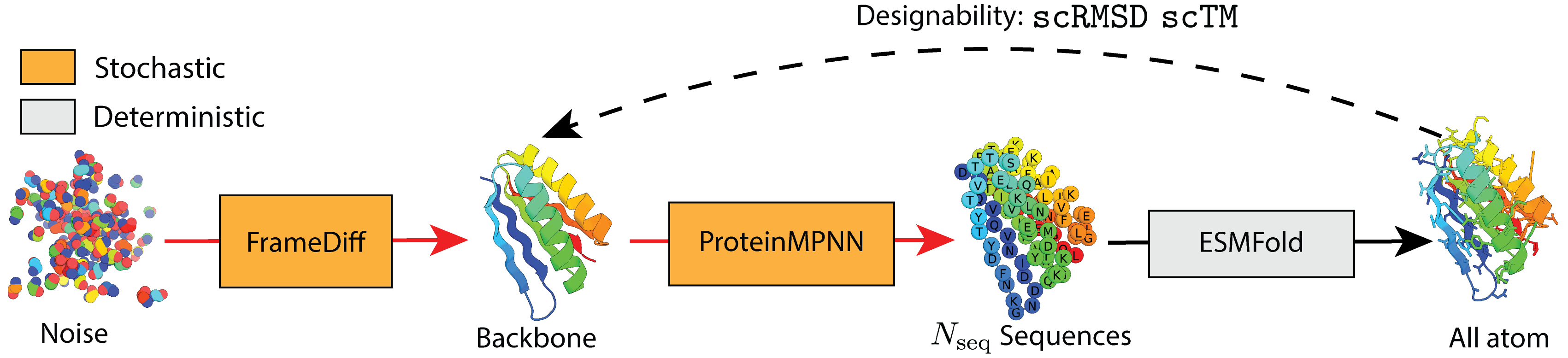
Figure 5: Designability test. Using $\mathrm{FrameDiff}$, we sample a backbone starting from noise then proceed to sample multiple ($N_{\mathrm{seq}}$) sequences with $\mathrm{ProteinMPNN}$(Dauparas et al., 2022). Each sequence is then folded with ESMFold (Lin et al., 2023) to obtain the predicted backbone which is scored again the sampled backbone with RMSD (scRMSD) or TM-score (scTM). This framework also gives a method for generating a full protein with sequence and sidechains starting from a generated backbone.

Designability. A generated backbone is meaningful only if there exists an amino acid sequence which folds to that structure. We follow Trippe et al. (2023) and assess backbone designability with self-consistency evaluation: a fixed-backbone sequence design algorithm proposes sequences, these sequences are input to a structure prediction algorithm, and self-consistency is assessed as the best agreement between the sampled and predicted backbones (see Fig. 5). In this work, we use $\mathrm{ProteinMPNN}$ at temperature 0.1 to generate $N_{\mathrm{seq}}$ sequences for $\mathrm{ESMFold}$ (Lin et al., 2023) to predict structures. We quantify self-consistency through both TM-score (scTM, higher is better) and $\texttt{C}_{\alpha}$-RMSD (scRMSD, lower is better). Chroma reports using scTM$>0.5$ as the designable criterion. However, it was shown scRMSD$<2$Å provides a more stringent filter, particularly for long (e.g. 600 amino acid) backbones on which $0.75$ scTM can be attained for very structurally different backbones (Watson et al., 2022).

Diversity. We quantify the diversity of backbones sampled by $\mathrm{FrameDiff}$ through the number of distinct structural clusters. In particular, for a collection of backbone samples we use MaxCluster (Herbert & Sternberg, 2008) to hierarchically cluster backbones with a 0.5 TM-score threshold. We report diversity as the proportion of unique clusters: (number of clusters) / (number of samples).

Novelty. We assess the ability of $\mathrm{FrameDiff}$ to generalize beyond the training set and produce novel backbones by comparing the similarity to known structures in the PDB. We use FoldSeek (van Kempen et al., 2023) to search for similar structures and report the highest TM-scores of samples to any chain in PDB, which we refer to as pdbTM.

5.2 Results

We analyze $\mathrm{FrameDiff}$ monomer samples on designability, diversity, and novelty. On designability, we briefly compare $\mathrm{FrameDiff}$’s samples with backbone generation diffusion models Chroma and RFdiffusion. However, we note that the training and evaluation set-ups are significantly different across $\mathrm{FrameDiff}$, Chroma, and RFdiffusion.

Using scTM$>0.5$ as the designable criterion, Chroma reported designability of 55% with 100 designed sequences ($N_{\mathrm{seq}}=100$). Lengths are between 100 and 500 and sampled proportionally “1/length”. However, this heavily biases performance towards shorter lengths and leads to additional length variability across evaluations. Instead, we sample 10 backbones at every length [100, 105, …, 495, 500] in intervals of 5 (810 total samples) such that lengths are fixed and distributed uniformly.

Table 1 reports $\mathrm{FrameDiff}$ metrics as we vary different sampling parameters. We notice a stark improvement in designability by changing the noise scale $\zeta=0.5$ at the cost of lower diversity. Increasing $N_{\mathrm{seq}}$ also improves designability but at a significant compute cost. The reported results use $N_{\mathrm{steps}}=500$; however decreasing to $N_{\mathrm{steps}}=100$ with a low noise scale still resulted in designable backbones. With $N_{\mathrm{steps}}=100$, generation of a 100 amino acid backbone takes 4.4 seconds on an A100 GPU; compared to RFdiffusion, this is more than an order of magnitude speed-up.

Table 1: $\mathrm{FrameDiff}$ sample metrics.

Noise scale $\zeta$	1.0	0.5	0.1	0.1	0.1
$N_{\text{steps}}$	500	500	500	500	100
$N_{\text{seq}}$	8	8	8	100	8
$>0.5$ scTM ($\uparrow$)	49%	74%	75%	84%	74%
$<2$Å scRMSD ($\uparrow$)	11%	23%	28%	40%	24%
Diversity ($\uparrow$)	0.75	0.56	0.53	0.54	0.55

Using $\zeta=1.0$, $N_{\mathrm{steps}}=500$, $N_{\mathrm{seq}}=8$, we perform ablations on self-conditioning, auxiliary losses, and form of the $\mathrm{SO}(3)$ loss – either the DSM form developed in our work or the squared Frobenius norm loss ($\mathcal{L}_{F}$, equal to $\|\hat{R}^{(0)}-R^{(0)}\|_{F}^{2}$) used in prior works (Watson et al., 2022; Luo et al., 2022). Our results are in Table 2 where we see the best model incorporates all components. We leave hyperparameter searches to future work.

Table 2: $\mathrm{FrameDiff}$ ablations.

$>0.5$scTM ($\uparrow$)	Self cond.	$\mathcal{L}_{\mathrm{2D}}$	$\mathcal{L}_{\mathrm{bb}}$	$\mathcal{L}_{\mathrm{dsm}}$	$\mathcal{L}_{F}$
49%	✓	✓	✓	✓
39%	✓	✓	✓		✓
42%		✓	✓	✓
22%			✓	✓
16%				✓
0%	✓	✓	✓

In Fig. 3A, we evaluate scRMSD across four lengths. $\mathrm{FrameDiff}$ is able to generate designable samples without pretraining; by contrast, RFdiffusion demonstrated the capacity to generate designable sequences only when initialized with pre-trained weights. More training data (i.e. training on complexes) and neural network parameters could help close the gap to RFdiffusion’s reported performance. Finally, RFdiffusion uses an all-to-all pairwise TM-align to measure diversity of its samples with clustering at 0.6 TM-score threshold. We perform an equivalent diversity evaluation using maxcluster with 0.6 TM-score threshold in Table 3 where we find a high degree of diversity ($>$0.5) that is comparable with RFdiffusion. Sec. J.4 shows more results and visualizations.

We next investigated the similarity of each sample to known structures in PDB. In Fig. 3B, we plot the novelty (pdbTM) as a function of designability (scRMSD). As expected, designability decreases with longer lengths. Samples with low scRMSD tend to have high similarity with the PDB. Our interest is in the lower left hand quadrant where scRMSD $<2.0$ and pdbTM $<0.6$. Fig. 3C illustrates two examples of $\mathrm{FrameDiff}$ samples that are designable and novel. We additionally find ESMFold to be highly confident, predicted LDDT (pLDDT) $>0.7$, for these samples.

Our experiments indicate $\mathrm{FrameDiff}$ is capable of learning complex distributions over protein monomer backbone that are designable, diverse, and in some cases novel compared to known protein structures. When used with decreased noise-scale, $75\%$ of samples across a range of lengths were designable by scTM${>}0.5;$ by contrast, all prior works reporting this metric not involving pretrained networks (see Sec. 6) have reported below 55% designability. However, due to differences in training and evaluation across these methods and ours, we refrain making state-of-the-art claims.

6 Related work

Diffusion models on proteins. Past works have developed diffusion models over different representations of protein structures without pretraining (Wu et al., 2022; Trippe et al., 2023; Anand & Achim, 2022; Qiao et al., 2022). Out of these methods, Chroma (Ingraham et al., 2022) reported the highest designability metric by diffusing over backbone atoms with a non-isotropic diffusion based on statistically determined covariance constraints. Compared to these works, we develop a principled $\mathrm{SE}(3)$ diffusion framework over protein backbones that demonstrates improved sample quality over methods that do not use $\mathrm{SE}(3)$ diffusion. Most similar to our work is RFdiffusion (Watson et al., 2022) which formulated the same forward diffusion process over $\mathrm{SE}(3)^{N}$, but with squared Frobenius norm rotation loss and reverse step that deviates from theory. We discuss the nuance between the rotation losses in Sec. I.5. While not outperforming RFdiffusion, FrameDiff enjoys several benefits such as being principled, having 1/4 the number of neural network weights, and not requiring expensive pretraining on protein structure prediction.

Diffusion models on manifolds. A general framework for continuous diffusion models on manifolds was first introduced in De Bortoli et al. (2022) extending the work of Song et al. (2021) to Riemannian manifolds. Concurrently, Huang et al. (2022) introduced a similar framework extending the maximum likelihood approach of Huang et al. (2021). Some manifolds have been considered in the setting of diffusion models for specific applications. In particular, Jing et al. consider the product of tori for molecular conformer generation, Corso et al. (2023) on the product space $\mathbb{R}^{3}\times\mathrm{SO}(3)\times\mathrm{SO}(2)^{m}$ for protein docking applications and Leach et al. (2022) on $\mathrm{SO}(3)$ for rotational alignment. Finally, we highlight the work of Urain et al. (2022) who introduce $\mathrm{SE}(3)$-diffusion models for robotics applications. One major theoretical and methodological difference with the present work is that we develop a principled diffusion model on this Lie group ensuring that at optimality we recover the exact backward process.

7 Discussion

Protein backbone generation is a fundamental task in de novo protein design. Motivated by the success of rigid-body frame representation of proteins, we developed an $\mathrm{SE}(3)$-invariant diffusion models on $\mathrm{SE}(3)^{N}$ for protein modelling. We laid the theoretical foundations of this method, and introduced $\mathrm{FrameDiff}$, a instance of this framework, equipped with an $\mathrm{SE}(3)$-equivariant score network which needs not to be pretrained. We empirically demonstrated $\mathrm{FrameDiff}$’s ability to generate designable and diverse samples. Even with stringent filters, we find our samples can generalize beyond PDB, although we note that claims of generating novel proteins requires experimental characterization. Our results are competitive with those reported in Chroma and RFdiffusion. However, differences in training and evaluation confound rigorous comparisons between the methods.

One important research direction is to extend $\mathrm{FrameDiff}$ to conditional generative modeling tasks, such as probabilistic sequence-to-structure prediction which to capture functional motion (Lane, 2023) and probabilistic scaffolding design given a functional motif (Trippe et al., 2023) We hypothesize scaling $\mathrm{FrameDiff}$ to train on larger data and improving the optimization would deliver backbones with designability on par with RFdiffusion while maintaining $\mathrm{FrameDiff}$’s simplicity. Finally, we highlight that the key aspects of our theoretical contributions— the general form of Brownian motions that is amenable to DSM along with sub-group invariance—are applicable to general Lie groups. Of particular interest are $\mathrm{SO}(3)$ in robotics (Barfoot et al., 2011) and $\mathrm{SU}(2)$ in Lattice QCD (Albergo et al., 2021).

Supplementary to:

$\mathrm{SE}(3)$ diffusion model

with application to protein backbone generation

Appendix A Organization of the supplementary

In this supplementary, we first recall in App. B some important concepts on Lie groups and representation theory which are useful for what follows. In App. C we derive the irreducible representations of $\mathrm{SU}(2)$ and then of $\mathrm{SO}(3)$. Using these, we introduce in App. D the canonical (bi-invariant) metric on $\mathrm{SO}(3)$, and a left-invariant metric on $\mathrm{SE}(3)$ which induces a Laplacian that factorises over $\mathrm{SO}(3)$ and $\mathbb{R}^{3}$. In particular, we prove Prop. 3.1. In App. E, we compute the heat kernel on compact Lie groups and in particular on $\mathrm{SO}(3)$, therefore proving Prop. 3.2 and Prop. 3.3. In App. F, we show that equivariant drift and diffusion coefficients induces invariant processes and prove Prop. 3.6. In App. G, we show the equivalence $\mathrm{SE}(3)$-invariant measures and $\mathrm{SO}(3)$-invariant measures with pinned center of mass, proving Prop. 3.5. Details about score computations on $\mathrm{SO}(3)$ using Rodrigues’ formula are given in App. H, including the proof of Prop. 3.4. In App. I, we include additional method details. In App. J, we present additional experiment details.

Appendix B Lie group and representation theory toolbox

In this section, we introduce some useful tools for the study of the heat kernel on Lie groups using representation theory. We refer to (Faraut, 2008; Hall, 2015; Harris et al., 1991; Knapp & Knapp, 1996; Folland, 2016) for more details on Lie groups and representation theory.

B.1 Group representation

Let $G$ be a group. A group representation $(\rho,V)$ is given by a vector space $V$ and a homomorphism $\rho:\ G\to\mathrm{GL}(V)$. A representation $(\rho,V)$ is said to be irreducible if for any subspace $W\subset V$ which is invariant by $\rho$, i.e. $\rho(G)(W)\subset W$, then $W=\{0\}$ or $W=V$. The study of irreducible group representations is at the heart of the analysis on groups. In particular, it is remarkable that if $G$ is compact every unitary representation can be decomposed as a direct sum of irreducible finite dimensional unitary representations of $G$. This result is known as the Peter–Weyl theorem (Weyl & Peter, 1927).

B.2 Lie group and Lie algebra

We recall that a Lie group is a group which is also a differentiable manifold for which the multiplication and inversion maps are smooth. Homomorphism of Lie groups are homomorphisms of groups with an additional smoothness assumption. The Lie algebra of a Lie group $G$ is defined as the tangent space of the Lie group at the identity element $\mathbf{e}$ and is denoted $\mathfrak{g}$. A vector field $X\in\mathfrak{X}(G)$ acts on a smooth function $f\in\mathrm{C}^{\infty}(G)$ as $X(f)=\sum_{i=1}^{d}X_{i}\partial_{i}f$. Note that $X(f)\in\mathrm{C}^{\infty}(G)$. Given two vector fields $X,Y\in\mathfrak{X}(G)$, the bracket between $X$ and $Y$ is given by $[X,Y]\in\mathfrak{X}(G)$ such that for any $f\in\mathrm{C}^{\infty}(G)$, $[X,Y](f)=X(Y(f))-Y(X(f))$. Note that for any $X_{0}\in\mathfrak{g}$ there exists $X\in\mathfrak{X}(G)$ such that $X(\mathbf{e})=X_{0}$. Hence, we define the Lie bracket between $X_{0},Y_{0}\in\mathfrak{g}$ as $[X_{0},Y_{0}]=[X,Y]$. Note that if $G\subset\mathrm{GL}_{n}(\mathbb{C})$ then we have that for any $X,Y\in\mathfrak{g}$, $[X,Y]=XY-YX$, where $XY$ is the matrix product between $X$ and $Y$.

For an arbitrary Lie group, the exponential mapping is defined as $\exp:\ \mathfrak{g}\to G$ such that for any $X\in\mathfrak{g}$, $\exp[X]=\gamma(1)$ where $\gamma:\ \mathbb{R}\to G$ is an homomorphism such that $\gamma^{\prime}(0)=X$. Another useful exponential map in the space of matrices is the exponential of matrix, given by $\exp[X]=\sum_{k\in\mathbb{N}}X^{k}/k!$. Note that if the metric is bi-invariant (invariant w.r.t. the left and right actions) then the associated exponential map coincides with the exponential of matrix, see (Carmo, 1992, Chapter 3, Exercise 3). If $G$ is compact then given any left-invariant metric $\langle\cdot,\cdot\rangle_{G}$ we can consider $\langle\cdot,\cdot\rangle_{\bar{G}}$ given for any $X,Y\in\mathfrak{G}$ by

$$\textstyle{\langle X,Y\rangle_{\bar{G}}=\int_{G}\langle\mathrm{d}R_{g}X,\mathrm{d}R_{g}Y\rangle\mathrm{d}\mu(g),}$$ (21)

where $\mu$ is the left-invariant Haar measure on $G$. Then $\langle\cdot,\cdot\rangle_{\bar{G}}$ is bi-invariant. If $G$ is compact and connected then $\exp$ is surjective, see Hall (2015, Exercises 2.9, 2.10).

One of the most important aspect of Lie groups is that (at least in the connected setting), they can be described entirely by their Lie algebra. More precisely, for any homomorphism $\Phi:\ G\to H$, denoting $\phi=\mathrm{d}\Phi(\mathbf{e}):\ \mathfrak{g}\to\mathfrak{h}$, we have $\Phi\circ\exp=\exp\circ\phi$, see Harris et al. (1991, p.105).

B.3 Lie algebra representations

A Lie algebra homomorphism $\phi:\ \mathfrak{g}\to\mathfrak{g}^{\prime}$ between two Lie algebras $\mathfrak{g}$ and $\mathfrak{g}^{\prime}$ is defined as a linear map which preserves Lie brackets, i.e. for any $X,Y\in\mathfrak{g}$, $\phi([X,Y])=[\phi(X),\phi(Y)]$. A Lie algebra representation of $\mathfrak{g}$ is given by $(\rho,V)$ such that $\rho:\ \mathfrak{g}\to\mathfrak{gl}(V)$ is a Lie algebra homomorphism, i.e. for any $X,Y\in\mathfrak{g}$, $\rho([X,Y])=\rho(X)\rho(Y)-\rho(Y)\rho(X)$. One way to construct Lie algebra representations is through Lie group representations. Indeed, one can verify that the differential at $\mathbf{e}$ of any Lie group representation is a Lie algebra representation.

One important Lie algebra representation is given by the adjoint representation. First, define $\Phi:\ G\to\mathrm{Aut}(G)$ such that for any $g,h\in G$, $\Phi(g)(h)=ghg^{-1}$. Then, for any $g\in G$, denote $\mathrm{Ad}(g)=\mathrm{d}\Phi(g)(\mathbf{e})$. Note that for any $g\in G$, we have that $\mathrm{Ad}(g)\in\mathrm{GL}(\mathfrak{g})$. $\mathrm{Ad}:\ G\to\mathrm{GL}(\mathfrak{g})$ is a Lie homomorphism and therefore a representation of $G$. Differentiating the adjoint Lie group representation we obtain a Lie algebra representation $\mathrm{ad}:\ \mathfrak{g}\to\mathfrak{gl}(\mathfrak{g})$. It can be shown that for any $X,Y\in\mathfrak{g}$, $\mathrm{ad}(X)(Y)=[X,Y]$. Note that we have $\mathrm{Ad}\circ\exp=\exp\circ\mathrm{ad}$ (Hall, 2015, Chapter 2, Proposition 2.24, Exercise 19). Note that this equivalence between homomorphism defined on the group level and homomorphisms defined on the Lie algebra level can be extended in the simply connected setting, see (Hall, 2015, Theorem 3.7).

Appendix C Representations and characters of $\mathrm{SO}(3)$

In order to study the irreducible (unitary) representations of $\mathrm{SO}(3)$, we first focus on the irreducible (unitary) representations of $\mathrm{SU}(2)$ in Sec. C.1. We describe the double-covering of $\mathrm{SO}(3)$ by $\mathrm{SU}(2)$, which relates these two groups, in Sec. C.2. We discuss different $\mathrm{SO}(3)$ parameterizations in Sec. C.3. Finally, we give the $\mathrm{SO}(3)$ irreducible unitary representations in Sec. C.4.

C.1 Representations and characters of $\mathrm{SU}(2)$

In this section, we follow the presentation of Faraut (2008) and provide a construction of the irreducible unitary representations of $\mathrm{SU}(2)$ for completeness. We refer to Faraut (2008); Hall (2015) for an extensive study of this group. For every $m\in\mathbb{N}$, with $n\geq 1$ we consider the representation $(\pi_{m},V_{m})$ where $V_{m}$ is the space of homogeneous polynomials of degree $m$ with two variables $X$, $Y$ and complex coefficients. For any $P\in V_{m}$ and $g\in\mathrm{SL}(2,\mathbb{C})$, we define $\pi_{m}(g)(P)(X,Y)=P(g(X,Y))$. For example, we have

$$g=\left(\begin{matrix}0&-1\\ 1&0\end{matrix}\right),\qquad\pi_{4}(g)(X^{3}Y-X^{2}Y^{2})=-XY^{3}-X^{2}Y^{2}.$$ (22)

We denote $\rho_{m}$ the differentiated representation arising from $\pi_{m}:\ \mathfrak{sl}(2,\mathbb{C})\to\mathfrak{gl}(V_{m})$. A basis of $\mathfrak{sl}(2,\mathbb{C})$ (as a complex Lie algebra) is given by

$$H=\left(\begin{matrix}1&0\\ 0&-1\end{matrix}\right),\qquad E=\left(\begin{matrix}0&1\\ 0&0\end{matrix}\right),\qquad F=\left(\begin{matrix}0&0\\ 1&0\end{matrix}\right).$$ (23)

We have the following Lie brackets

$$[H,E]=2E,\qquad[H,F]=-2F,\qquad[E,F]=H.$$ (24)

A basis of $V_{m}$ is given by $\{P_{j}\}_{j=0}^{m}$ with $P_{j}=X^{j}Y^{m-j}$ for $j\in\{0,\dots,m\}$. Using (Hall, 2015, Theorem 3.7), we have that $\rho_{m}(M)=(\exp[\pi_{m}(tM)])^{\prime}_{t=0}$, for $M\in\{E,F,H\}$ and therefore

$$\rho_{m}(H)(P)=X\partial_{X}P-Y\partial_{Y}P,\qquad\rho_{m}(E)(P)=X\partial_{Y}P,\qquad\rho_{m}(F)(P)=Y\partial_{X}P.$$ (25)

Proposition C.1.

For any $m\in\mathbb{N}$ with $m\geq 1$, $\rho_{m}$ is an irreducible Lie algebra representation.

Proof.

For any $j\in\{0,\dots,m\}$ we have

$$\rho_{m}(H)(P_{j})=(2j-m)P_{j},\qquad\rho_{m}(E)(P_{j})=(m-j)P_{j+1},\qquad\rho_{m}(F)(P_{j})=jP_{j-1},$$ (26)

with $P_{-1}=P_{m+1}=0$. Now let $W\neq\{0\}$ be an invariant subspace of $V_{m}$ for $\rho_{m}$. We have that $\rho_{m}(H)$ restricted to $W$ admits an eigenvector and therefore, there exists $j_{0}\in\{0,\dots,m\}$ such that $P_{j_{0}}\in W$. Indeed, let $P=\sum_{i=0}^{m}\alpha_{i}P_{i}$, with $(\alpha_{i})_{i=0}^{m}\in\mathbb{C}^{m+1}$, be such an eigenvector with eigenvalue $\lambda\in\mathbb{C}$. We have

$$\textstyle{\sum_{i=0}^{m}(2i-m)\alpha_{i}P_{i}=\rho_{m}(H)(P)=\sum_{i=0}^{m}\lambda\alpha_{i}P_{i}.}$$ (27)

Hence, $\sum_{i=0}^{m}(2i-m-\lambda)\alpha_{i}P_{i}=0$. This means that for any $i\in\{0,\dots,m\}$ except for one $i_{0}\in\{0,\dots,m\}$, $\alpha_{i}=0$. Hence, $P_{i_{0}}\in W$. Upon applying $\rho_{m}(E)$ and $\rho_{m}(F)$ repeatedly we find that for any $j\in\{0,\dots,m\}$, $P_{j}\in W$ and therefore $W=V_{m}$, which concludes the proof. ∎

Proposition C.2.

Let $(\rho,V)$ an irreducible Lie algebra representation, then there exist $m\in\mathbb{N}$ with $m\geq 1$ and $A\in\mathrm{GL}(V,V_{m})$ such that for any $\rho=A^{-1}\rho_{m}A$.

Proof.

Let $v$ be the eigenvector of $\rho(H)$ associated with eigenvalue $\lambda$ with smallest real part. Using (24), we have that

$$\rho(H)\rho(E)v=\rho(E)\rho(H)v+\rho([H,E])v=(\lambda+2)\rho(E)v.$$ (28)

Similarly, we have

$$\rho(H)\rho(F)v=\rho(F)\rho(H)v+\rho([H,F])v=(\lambda-2)\rho(F)v.$$ (29)

For any $k\in\mathbb{N}$, denote $v_{k}=\rho(E)^{k}v$. Denote $m\in\mathbb{N}$ such that for any $k>m$, $v_{k}=0$ and $v_{m}\neq 0$. We have that $\{v_{0},\dots,v_{m}\}$ are linearly independent, since for each $k\in\{0,\dots,m\}$ we have that $v_{k}$ is an eigenvector of $\rho(H)$ with eigenvalue $\lambda+2k$. Denote $W$ the subspace spanned by $\{v_{0},\dots,v_{m}\}$. $\rho(H)(W)\subset W$ and $\rho(E)(W)\subset W$. Let us show that $\rho(F)(W)\subset W$. Assume that $\rho(F)v_{k}=\alpha_{k}v_{k-1}$ for some $k\in\{1,\dots,m-1\}$, then we have

$$\rho(F)(v_{k+1})=\rho(F)\rho(E)v_{k}=\rho(E)\rho(F)v_{k}+\rho([F,E])v_{k}=(\alpha_{k}-(\lambda+2k))v_{k}.$$ (30)

Hence, setting $\alpha_{k+1}=\alpha_{k}-(\lambda+2k)$, we get that that $\rho(F)(v_{k+1})=\alpha_{k+1}v_{k}$. Let us show that $\rho(F)(v_{1})=\alpha_{1}v_{0}=-\lambda v_{0}$. First, using (29) we have that if $\rho(F)(v_{0})\neq 0$ then $\rho(F)(v_{0})$ is an eigenvector of $\rho(H)$ for the eigenvalue $\lambda-2$, which is absurd since $\lambda$ has minimal real part. Hence $\rho(F)(v_{0})=0$ and we have

$$\rho(F)(v_{1})=\rho(E)\rho(F)v_{0}+\rho([F,E])v_{0}=-\lambda v_{0}.$$ (31)

Therefore, we have that $\rho(F)(W)\subset W$ and therefore $V=W$ since $\rho$ is irreducible. In addition, by recursion, we have that for any $k\in\{0,\dots,m\}$, $\alpha_{k}=-k(\lambda+k-1)$. A basis of $V$ is given by $\{v_{j}\}_{j=0}^{m}$ and we have that for any $j\in\{0,\dots,m\}$

$$\rho(H)(v_{j})=(\lambda+2j)v_{j},\qquad\rho(E)(v_{j})=v_{j+1},\qquad\rho(F)(v_{j})=-j(\lambda+j-1)v_{j-1},$$ (32)

with $v_{-1}=v_{m+1}=0$. We have that

$$\textstyle{\operatorname{Tr}(\rho(H))=0=\sum_{j=0}^{m}\lambda+2j=(m+1)(\lambda+m)}.$$ (33)

Hence $\lambda=-m$ and we have

$$\rho(H)(v_{j})=(-m+2j)v_{j},\qquad\rho(E)(v_{j})=v_{j+1},\qquad\rho(F)(v_{j})=j(m-j+1)v_{j-1},$$ (34)

Hence, letting $w_{j}=\lambda_{j}v_{j}$ with $\lambda_{j}/\lambda_{j+1}=m-j$ we have

$$\rho(H)(w_{j})=(-m+2j)w_{j},\qquad\rho(E)(w_{j})=(m-j)w_{j+1},\qquad\rho(F)(w_{j})=jw_{j-1}.$$ (35)

We conclude upon defining $Aw_{j}=P_{j}$ for any $j\in\{0,\dots,m\}$. ∎

Proposition C.3.

Let $(\pi,V)$ be a irreducible representation of $\mathrm{SU}(2)$ then there exist $m\in\mathbb{N}$ and $A\in\mathrm{GL}(V,V_{m})$ such that $\pi=A^{-1}\pi_{m}A$.

Proof.

Let $\rho:\ \mathfrak{su}(2)\to\mathfrak{gl}(V)$ the Lie algebra representation associated with $\pi$. $\rho$ can be linearly extended to a Lie algebra representation of $\mathfrak{sl}(2,\mathbb{C})$ using that $\mathfrak{sl}(2,\mathbb{C})=\mathfrak{su}(2)\oplus\mathfrak{su}(2)$ (indeed each element $Z$ of $\mathfrak{sl}(2,\mathbb{C})$ can be written uniquely as $Z=X+\emph{i}Y$ with $X,Y\in\mathfrak{su}(2)$). The extension of $\rho$ is given by $\rho_{\mathrm{ext}}(Z)=\rho(X)+\emph{i}\rho(Y)$. Let $W$ be an invariant subspace for $\rho_{\mathrm{ext}}$ then it is an invariant subspace for $\rho$ and therefore for any $X\in\mathfrak{su}(2)$, $\exp[\rho(X)](W)\subset W$. Using that $\mathrm{SU}(2)$ is connected we have that for any $U\in\mathrm{SU}(2)$ there exists $X\in\mathfrak{su}(2)$ such that $U=\exp[X]$ and using that $\pi\circ\exp=\exp\circ\rho$, (Hall, 2015, Theorem 3.7), we get that $\pi(\mathrm{SU}(2))(W)\subset W$ and therefore $W=V$. Hence, $\rho_{\mathrm{ext}}$ is irreducible and there exist $m\in\mathbb{N}$ and $A\in\mathrm{GL}(V,V_{m})$ such that $\rho=A^{-1}\rho_{m}A$. We conclude by exponentiation, (Hall, 2015, Theorem 3.7). ∎

C.2 Double-covering of $\mathrm{SO}(3)$

In order to derive the (unitary) irreducible representations of $\mathrm{SO}(3)$ we first link $\mathrm{SO}(3)$ with $\mathrm{SU}(2)$ using the adjoint representation. First, let us consider a basis of $\mathfrak{su}(2)$, $(X_{1},X_{2},X_{3})$ given by

$$X_{1}=\left(\begin{matrix}0&\emph{i}\\ \emph{i}&0\end{matrix}\right),\qquad X_{2}=\left(\begin{matrix}0&-1\\ 1&0\end{matrix}\right),\qquad X_{3}=\left(\begin{matrix}\emph{i}&0\\ 0&-\emph{i}\end{matrix}\right).$$ (36)

A basis of $\mathfrak{so}(3)$ is given by

$$Y_{1}=\left(\begin{matrix}0&0&0\\ 0&0&-1\\ 0&1&0\end{matrix}\right),\qquad Y_{2}=\left(\begin{matrix}0&0&1\\ 0&0&0\\ -1&0&0\end{matrix}\right),\qquad Y_{3}=\left(\begin{matrix}0&-1&0\\ 1&0&0\\ 0&0&0\end{matrix}\right).$$ (37)

Note that for any $i\in\{1,2,3\}$, $\mathrm{ad}(X_{i})=2Y_{i}$, when represented in the basis $(X_{1},X_{2},X_{3})$ (recall that $\mathrm{ad}:\mathfrak{g}\to\mathfrak{gl}(\mathfrak{g})$). Therefore, we have that $\mathrm{ad}:\ \mathfrak{su}(2)\to\mathfrak{so}(3)$ is an isomorphism. Since $\mathrm{SO}(3)$ is compact and connected, $\exp$ is surjective and therefore using that $\mathrm{Ad}\circ\exp=\exp\circ\mathrm{ad}$, we get that $\mathrm{Ad}:\ \mathrm{SU}(2)\to\mathrm{SO}(3)$ is surjective. In addition, we have that $\mathrm{Ker}(\mathrm{Ad})=\{\pm\mathbf{e}\}$. Hence $\mathrm{SU}(2)$ is a double-covering of $\mathrm{SO}(3)$.

C.3 Parameterizations of $\mathrm{SO}(3)$

Before concluding this section and describing the unitary representations of $\mathrm{SO}(3)$, we describe different possible parameterizations of $\mathrm{SO}(3)$ and its Lie algebra.

Axis-angle.

Let $(a,b,c)\in\mathbb{R}^{3}$ such that $a^{2}+b^{2}+c^{2}=1$, i.e. $\bm{\omega}=(a,b,c)\in\mathbb{S}^{2}$ and $\theta\in\mathbb{R}_{+}$, then any element of $\mathfrak{so}(3)$ is given by $Y=\theta K$, with $K=aY_{1}+bY_{2}+cY_{3}$. Hence, any element of $\mathrm{SO}(3)$ can be written as $\exp[\theta K]$. The parameterization of $\mathrm{SO}(3)$ using $(\bm{\omega},\theta)$ is called the axis-angle parameterization. Using that $K^{3}=-K$ we have

$$\exp[\theta K]=\operatorname{Id}+\sin(\theta)K+(1-\cos(\theta))K^{2}.$$ (38)

This is called the Rodrigues’ formula and provides a concise way of computing the exponential. In addition, it should be noted that for any $(a,b,c),v\in\mathbb{R}^{3}$,

$$(aY_{1}+bY_{2}+cY_{3})v=a\times v,\qquad(aY_{1}+bY_{2}+cY_{3})^{2}v=\langle a,v\rangle a-v.$$ (39)

Combining this result (39) we recover the Rodrigues’ rotation formula, i.e. for any $\bm{v}\in\mathbb{R}^{3}$ we have

$$\exp[\theta K]\bm{v}=\cos(\theta)\bm{v}+\sin(\theta)\bm{\omega}\times\bm{v}+(1-\cos(\theta))\langle\bm{\omega},\bm{v}\rangle\bm{\omega}.$$ (40)

From this formula, it can be seen that $\exp[\theta K]\bm{v}$ is the rotation of the vector $\bm{v}$ of angle $\theta$ around the axis $\bm{\omega}$.

Euler angles.

For every $U\in\mathrm{SU}(2)$ there exists $(\psi,\theta,\varphi)\in\mathbb{R}^{3}$ such that $U=\exp[\psi X_{3}]\exp[\theta X_{2}]\exp[\varphi X_{3}]$. Therefore, using that $\mathrm{Ad}$ is surjective and that $\mathrm{Ad}\circ\exp=\exp\circ\mathrm{ad}$ we have that for any $R\in\mathrm{SO}(3)$ there exists $(\psi,\theta,\varphi)\in\mathbb{R}^{3}$ such that

$$R =\exp[\psi Y_{3}]\exp[\theta Y_{1}]\exp[\varphi Y_{3}]$$ (41)

$$=\left(\begin{matrix}\cos(\psi)&-\sin(\psi)&0\\ \sin(\psi)&\cos(\psi)&0\\ 0&0&1\end{matrix}\right)\left(\begin{matrix}1&0&0\\ 0&\cos(\theta)&-\sin(\theta)\\ 0&\sin(\theta)&\cos(\theta)\end{matrix}\right)\left(\begin{matrix}\cos(\varphi)&-\sin(\varphi)&0\\ \sin(\varphi)&\cos(\varphi)&0\\ 0&0&1\end{matrix}\right).$$ (42)

The three angles $\psi,\theta,\varphi$ are called the Euler angles: $\psi$ is called the precession angle, $\theta$ the nutation angle and $\varphi$ the angle of proper rotation (or spin).

Quaternions.

Every element $U$ of $\mathrm{SU}(2)$ can be uniquely written as

$$U=\left(\begin{matrix}\alpha&\beta\\ -\bar{\beta}&\alpha\end{matrix}\right),$$ (43)

with $\alpha,\beta\in\mathbb{C}^{2}$ and $\left|\alpha\right|^{2}+\left|\beta\right|^{2}=1$. This representation of $\mathrm{SU}(2)$ entails an isomorphism between $\mathrm{SU}(2)$ and the unit sphere in $\mathbb{R}^{4}$, which shows that $\mathrm{SU}(2)$ is simply connected. To draw the link with quaternions, we introduce $\bm{i}=X_{1}$, $\bm{j}=-X_{2}$ and $\bm{k}=X_{3}$. Note that $\bm{i}^{2}=\bm{j}^{2}=\bm{k}^{2}=\bm{ijk}=-1$. Using the exponential map and the properties of $\bm{i},\bm{j}$ and $\bm{k}$, we get that each element in $\mathrm{SU}(2)$ can be uniquely represented as $q=a+b\bm{i}+c\bm{j}+d\bm{k}$ with $\left\lVert q\right\rVert^{2}=a^{2}+b^{2}+c^{2}+d^{2}=1$. Using the adjoint representation, we get that $\mathrm{Ad}(q)$ is the rotation with axis $(b,c,d)$ and angle $\theta$ such that $\tan(\theta/2)=\sqrt{b^{2}+c^{2}+d^{2}}/\left|a\right|$ if $a\neq 0$ and $\theta=\pi$ otherwise.

C.4 Irreducible representations and characters of $\mathrm{SO}(3)$

We start by describing the irreducible characters of $\mathrm{SU}(2)$. Recall that irreducible unitary representations of $\mathrm{SU}(2)$ are given in Prop. C.3.

Proposition C.4.

Let $U\in\mathrm{SU}(2)$ such that $U=\exp[\theta X]$ with $X=aX_{1}+bX_{2}+cX_{3}$ and $a^{2}+b^{2}+c^{2}=1$, $\theta>0$. Then for any $m\in\mathbb{N}$ with $m\geq 1$ we have

$$\chi_{m}(U)=\sin((m+1)\theta)/\sin(\theta).$$ (44)

Proof.

First note that $X^{2}=-\operatorname{Id}$. Hence $\{-\emph{i}\theta,\emph{i}\theta\}$ are the eigenvalues of $\theta X$ and $\{\mathrm{e}^{\emph{i}\theta},\mathrm{e}^{-\emph{i}\theta}\}$ are the eigenvalues of $\exp[\theta X]$. Hence, there exists $U_{0}\in\mathrm{SU}(2)$ such that $U=U_{0}U_{\theta}U_{0}^{-1}$ with $U_{\theta}$ diagonal with values $\{\mathrm{e}^{\emph{i}\theta},\mathrm{e}^{-\emph{i}\theta}\}$. Hence, since $\chi_{m}$ is a trace class function we have that $\chi_{m}(U)=\chi_{m}(U_{\theta})$. We have that $\rho_{m}(\emph{i}\theta H)$ has eigenvalues $\{\emph{i}\theta(2j-m)\}_{j=0}^{m}$. Therefore, we get that $\pi_{m}(U_{\theta})$ has eigenvalues $\{\mathrm{e}^{\emph{i}\theta(2j-m)}\}_{j=0}^{m}$, using that $\exp\circ\rho_{m}=\pi_{m}\circ\exp$. We conclude upon summing the eigenvalues. ∎

Proposition C.5.

Let $(\pi,V)$ be an irreducible representation of $\mathrm{SO}(3)$. Then there exist $m\in\mathbb{N}$ with $m\geq 1$ and $A\in\mathrm{GL}(V,V_{m})$ such that $\pi\circ\mathrm{Ad}=A^{-1}\pi_{2m}A$. Respectively for any $m\in\mathbb{N}$, there exists $\tilde{\pi}_{m}$ such that $\tilde{\pi}_{m}\circ\mathrm{Ad}=\pi_{2m}$.

Proof.

Let $\pi$ be an irreducible representation of $\mathrm{SO}(3)$. Then $\pi\circ\mathrm{Ad}$ is an irreducible representation of $\mathrm{SU}(2)$ and therefore equivalent to $\pi_{m}$ for some $m\in\mathbb{N}$ with $m\geq 1$. Since $\mathrm{Ad}(-\mathbf{e})=\mathbf{e}$ we have that $m$ is even. Respectively, for any $m\in\mathbb{N}$ with $m\geq 1$, since $\pi_{2m}(-\mathbf{e})=\mathbf{e}$ then $\pi_{2m}$ factorizes through $\mathrm{Ad}$, which concludes the proof. ∎

Proposition C.6.

Let $R\in\mathrm{SO}(3)$ such that $R=\exp[\theta X]$ with $X=aY_{1}+bY_{2}+cY_{3}$ and $a^{2}+b^{2}+c^{2}=1$, $\theta>0$ (i.e. we consider the axis-angle representation of $R$). Then for any $m\in\mathbb{N}$ with $m\geq 1$, we have

$$\chi_{m}(R)=\sin((m+1/2)\theta)/\sin(\theta/2).$$ (45)

Proof.

Let $m\in\mathbb{N}$ with $m\geq 1$. The associated representation with $\chi_{m}$ is $\tilde{\pi}_{m}$ such that $\tilde{\pi}_{m}=\pi_{2m}\circ\mathrm{Ad}$. Let $X=aX_{1}+bX_{2}+cX_{3}$, we have that $\mathrm{Ad}(\exp[(\theta/2)X])=\exp[\theta Y]$. We conclude using Prop. C.4. ∎

We conclude this section by noting that $\mathrm{SO}(3)$ representations can also be realized with spherical harmonics (Faraut, 2008).

Appendix D Metrics and Laplacians

In this section, we provide more details on the metrics and Laplacian on $\mathrm{SE}(3)$. We start by introducing a canonical metric on $\mathrm{SO}(3)$ in Sec. D.1. Then, we move onto the parameterization of $\mathrm{SE}(3)$, its Lie algebra and adjoint representations in Sec. D.2. Once we have introduced these tools we describe one metric in Sec. D.3 which gives rises to the factorized formulation of the Laplacian. Finally, we conclude with considerations on the unimodularity of $\mathrm{SE}(3)$ in Sec. D.4.

D.1 Canonical metric on $\mathrm{SO}(3)$

We first describe a canonical metric on $\mathrm{SO}(3)$ obtained using the notion of Killing form. The construction of such a metric is valid for any compact Lie group.

Adjoint representations.

First, we need to compute the adjoint representation on $\mathrm{SO}(3)$. We recall that a basis of $\mathfrak{so}(3)$ is given by

$$Y_{1}=\left(\begin{matrix}0&0&0\\ 0&0&-1\\ 0&1&0\end{matrix}\right),\qquad Y_{2}=\left(\begin{matrix}0&0&1\\ 0&0&0\\ -1&0&0\end{matrix}\right),\qquad Y_{3}=\left(\begin{matrix}0&-1&0\\ 1&0&0\\ 0&0&0\end{matrix}\right).$$ (46)

We have that $[Y_{1},Y_{2}]=Y_{3}$, $[Y_{2},Y_{3}]=Y_{1}$ and $[Y_{3},Y_{1}]=Y_{2}$. We have the following result.

Proposition D.1.

$\mathrm{ad}=\operatorname{Id}$ and $\mathrm{Ad}=\operatorname{Id}$.

Proof.

Recalling that for any $i,j\in\{1,2,3\}$, $\mathrm{ad}(Y_{i})(Y_{j})=[Y_{i},Y_{j}]$ we obtain the result using the Lie bracket relations. We conclude upon using that $\mathrm{Ad}\circ\exp=\exp\circ\mathrm{ad}$ and that $\exp$ is surjective since $\mathrm{SO}(3)$ is compact and connected. ∎

Killing form.

We begin by recalling a few basics on the Killing form. The Killing form $B$ is a symmetric $2$-form on $\mathfrak{g}$ defined for any $X,Y\in\mathfrak{g}$ by

$$B(X,Y)=\operatorname{Tr}(\mathrm{ad}(X)\circ\mathrm{ad}(Y)).$$ (47)

One of the key property of the Killing form is that it is invariant under any automorphims of the Lie algebra. In particular, using that for any $g\in G$, $X,Y\in\mathfrak{g}$ and $g\in G$, $\mathrm{Ad}(g)[X,Y]=[\mathrm{Ad}(X),\mathrm{Ad}(Y)]$, we have

$$B(\mathrm{Ad}(g)(X),\mathrm{Ad}(g)(Y))=B(X,Y).$$ (48)

The invariance under the adjoint representation is key to define metrics which are bi-invariant (left and right invariant). Let $\bar{B}$ a positive symmetric $2$-form on $\mathfrak{g}$, i.e. a scalar product. Then $\bar{B}$ defines a left-invariant metric $\langle\cdot,\cdot\rangle$ on $G$ by letting for any $g\in G$ and $X,Y\in\mathrm{T}_{g}G$

$$\langle X_{g},Y_{g}\rangle_{G}=\bar{B}(\mathrm{d}L_{g}(\mathbf{e})^{-1}X_{g},\mathrm{d}L_{g}(\mathbf{e})^{-1}Y_{g}),$$ (49)

where $L_{g}:\ G\to G$ is given for any $h\in G$ by $L_{g}(h)=gh$.

Proposition D.2.

The metric $\langle\cdot,\cdot\rangle$ is right-invariant if and only if $\bar{B}$ is $\mathrm{Ad}(g)$-invariant for any $g\in G$.

Proof.

We have that $\langle\cdot,\cdot\rangle$ is right-invariant if for any $g,h\in G$ and $X_{h},Y_{h}\in\mathrm{T}_{h}G$,

$$\langle\mathrm{d}R_{g}(h)(X_{h}),\mathrm{d}R_{g}(h)(Y_{h})\rangle=\langle X_{h},Y_{h}\rangle.$$ (50)

We have that for any $g,h\in G$ and $X_{h},Y_{h}\in\mathrm{T}_{h}G$

$$\langle\mathrm{d}R_{g}(h)(X_{h}),\mathrm{d}R_{g}(h)(Y_{h})\rangle=\bar{B}(\mathrm{d}L_{hg}(\mathbf{e})^{-1}\mathrm{d}R_{g}(h)(X_{h}),\mathrm{d}L_{hg}(\mathbf{e})^{-1}\mathrm{d}R_{g}(h)(Y_{h}))$$ (51)

In addition, using that for any $g_{1},g_{2}\in G$, $L_{g_{1}}$ and $R_{g_{2}}$ commute, we have that for any $g,h\in G$ and $X_{h},Y_{h}\in\mathrm{T}_{h}G$

$$\mathrm{d}L_{hg}(\mathbf{e})^{-1}\mathrm{d}R_{g}(h) =\mathrm{d}L_{g^{-1}h^{-1}}(hg)\mathrm{d}R_{g}(h)$$ (52)

$$=\mathrm{d}L_{g^{-1}}(g)\mathrm{d}L_{h^{-1}}(hg)\mathrm{d}R_{g}(h)$$ (53)

$$=\mathrm{d}L_{g^{-1}}(g)\mathrm{d}R_{g}(e)\mathrm{d}L_{h^{-1}}(h)$$ (54)

$$=\mathrm{Ad}(g)\mathrm{d}L_{h^{-1}}(h)=\mathrm{Ad}(g)\mathrm{d}L_{h}(\mathbf{e})^{-1}.$$ (55)

Combining this result and (51) we get that for any $g,h\in G$ and $X_{h},Y_{h}\in\mathrm{T}_{h}G$

$$\langle\mathrm{d}R_{g}(h)(X_{h}),\mathrm{d}R_{g}(h)(Y_{h})\rangle=\bar{B}(\mathrm{Ad}(g)\mathrm{d}L_{h}(\mathbf{e})^{-1}X_{h},\mathrm{Ad}(g)\mathrm{d}L_{h}(\mathbf{e})^{-1}Y_{h}).$$ (56)

In addition, we have for any $h\in G$ and $X_{h},Y_{h}\in\mathrm{T}_{h}G$, $\langle X_{h},Y_{h}\rangle=\bar{B}(\mathrm{d}L_{h}(\mathbf{e})^{-1}X_{h},\mathrm{d}L_{h}(\mathbf{e})^{-1}Y_{h})$. Therefore, we have that $\langle\cdot,\cdot\rangle$ is right-invariant if and only if for any $g,h\in G$ and $X_{h},Y_{h}\in\mathrm{T}_{h}G$

$$\bar{B}(\mathrm{d}L_{h}(\mathbf{e})^{-1}X_{h},\mathrm{d}L_{h}(\mathbf{e})^{-1}Y_{h})=\bar{B}(\mathrm{Ad}(g)\mathrm{d}L_{h}(\mathbf{e})^{-1}X_{h},\mathrm{Ad}(g)\mathrm{d}L_{h}(\mathbf{e})^{-1}Y_{h}).$$ (57)

Hence, we get that $\langle\cdot,\cdot\rangle$ is right-invariant if and only if for any $g\in G$ and $X,Y\in\mathfrak{g}$,

$$\bar{B}(X,Y)=\bar{B}(\mathrm{Ad}(g)(X),\mathrm{Ad}(g)(Y)),$$ (58)

which concludes the proof. ∎

Combining this result and (48) we immediately get that if the Killing form defines a scalar product then the associated left-invariant metric is also right-invariant. In the case of $\mathrm{SO}(3)$ we have the following explicit formula for the Killing form.

Proposition D.3.

If $G=\mathrm{SO}(3)$ we have that $B(X,Y)=\operatorname{Tr}(XY)$. In the basis $(Y_{1},Y_{2},Y_{3})$ we have that $B=-2\operatorname{Id}$.

Proof.

The first result is a direct consequence of Prop. D.1. The second result is a consequence of the fact that $\operatorname{Tr}(Y_{i}Y_{j})=-2\updelta_{i,j}$ for $i,j\in\{1,2,3\}$. ∎

Hence by considering $-B/2$ we obtain that $\{Y_{1},Y_{2},Y_{3}\}$ is an orthonormal basis on $\mathfrak{so}(3)$. The associated metric is bi-invariant. We can define the Laplace-Beltrami operator associated with $\mathfrak{so}(3)$ and we have that for any $f\in\mathrm{C}^{\infty}(\mathrm{SO}(3))$ and $g\in\mathrm{SO}(3)$

$$\textstyle{\Delta f(g)=\sum_{i=1}^{3}\tfrac{\mathrm{d}}{\mathrm{d}t^{2}}f(g\exp[tY_{i}])|_{t=0}.}$$ (59)

Also, note that in that case the Riemannian exponential mapping coincide with the matrix exponential map, (Carmo, 1992, Chapter 3, Exercise 3).

Eigenvalues of the Laplacian.

Similarly, one can define $\Delta$ on $\mathrm{SU}(2)$ using the Killing form. In this case we have that $B(X,Y)=-\operatorname{Tr}(XY)$ and we set the metric on $\mathrm{SU}(2)$ to be the one associated with $-B/2$. We have that $\{X_{i}\}_{i=1}^{3}$ is an orthonormal basis of $\mathfrak{su}(2)$ for this metric and therefore for any $f\in\mathrm{C}^{\infty}(\mathrm{SU}(2))$ and $g\in\mathrm{SU}(2)$

$$\textstyle{\Delta f(g)=\sum_{i=1}^{3}\tfrac{\mathrm{d}}{\mathrm{d}t^{2}}f(g\exp[tX_{i}])|_{t=0},}$$ (60)

see (Faraut, 2008, p.162) for a definition and basic properties. It can be shown (Faraut, 2008, Proposition 8.2.1, Proposition 8.3.1) that for any $m\in\mathbb{N}$ with $m\geq 1$, we have

$$\Delta\chi_{m}=-m(m+2)\chi_{m}.$$ (61)

Using that $\mathrm{Ad}$ is surjective for any $g\in\mathrm{SO}(3)$ there exists $g_{0}\in\mathrm{SU}(2)$ such that $\mathrm{Ad}(g_{0})=g$. In addition, for any $i\in\{1,2,3\}$, $\mathrm{ad}(X_{i})=2Y_{i}$. Using these results and the fact that $\mathrm{Ad}\circ\exp=\exp\circ\mathrm{ad}$ we have that for any $f\in\mathrm{C}^{\infty}(\mathrm{SO}(3))$ and $g\in\mathrm{SO}(3)$

$$\Delta f(g) \textstyle{=\sum_{i=1}^{3}\tfrac{\mathrm{d}}{\mathrm{d}t^{2}}f(g\exp[tY_{i}])|_{t=0}}$$ (62)

$$\textstyle{=\sum_{i=1}^{3}\tfrac{\mathrm{d}}{\mathrm{d}t^{2}}f(g\exp[\mathrm{ad}(tX_{i}/2)])|_{t=0}}$$ (63)

$$\textstyle{=\sum_{i=1}^{3}\tfrac{\mathrm{d}}{\mathrm{d}t^{2}}f(g\mathrm{Ad}(\exp[tX_{i}/2]))|_{t=0}}$$ (64)

$$\textstyle{=\sum_{i=1}^{3}\tfrac{\mathrm{d}}{\mathrm{d}t^{2}}f(\mathrm{Ad}(g_{0}\exp[tX_{i}/2]))|_{t=0}}=\Delta(f\circ\mathrm{Ad})(g_{0})/4.$$ (65)

This result yields the following proposition.

Proposition D.4.

For every $m\in\mathbb{N}$, $\Delta\tilde{\chi}_{m}=-m(m+1)\tilde{\chi}_{m}$.

Proof.

Recall that for any $m\in\mathbb{N}$, $\chi_{2m}=\tilde{\chi}_{m}\circ\mathrm{Ad}$. Therefore, using (65), we have that for any $g\in\mathrm{SO}(3)$ and $m\in\mathbb{N}$

$$\Delta\tilde{\chi}_{m}(g)=\Delta\chi_{2m}(g_{0})/4=-m(m+1)\chi_{2m}(g_{0})=-m(m+1)\tilde{\chi}_{m}(g).$$ (66)

∎

D.2 Parameterization of $\mathrm{SE}(3)$ and Lie algebra

Parameterization.

The special Euclidean group on $\mathbb{R}^{3}$, denoted $\mathrm{SE}(3)$, (also known as the rigid body motion group, see (Murray et al., )) is the group given by all the affine isometries. We have

$$\mathrm{SE}(3)=\left\{\left(\begin{matrix}R&x\\ 0&1\end{matrix}\right)\,:R\in\mathrm{SO}(3),x\in\mathbb{R}^{3}\right\}.$$ (67)

As a consequence we have the following composition rule for $(R,x),(R^{\prime}x,^{\prime})\in\mathrm{SE}(3)$

$$(R,x)*(R^{\prime},x^{\prime})=(RR^{\prime},x+Rx^{\prime}).$$ (68)

Therefore as a group we have that $\mathrm{SE}(3)=\mathrm{SO}(3)\rtimes\mathbb{R}^{3}$. In particular, the group structure of $\mathrm{SE}(3)$ is different from the canonical product $\mathrm{SO}(3)\times\mathbb{R}^{3}$. The inverse of $(R,x)$ is given by $(R,x)^{-1}=(R^{-1},-R^{-1}x)$. $\mathrm{SE}(3)$ is also a $6$-dimensional Lie group and its Lie algebra is given by

$$\mathfrak{se}(3)=\left\{\left(\begin{matrix}X&x\\ 0&0\end{matrix}\right)\,:X\in\mathfrak{so}(3),x\in\mathbb{R}^{3}\right\}.$$ (69)

A basis for $\mathfrak{se}(3)=\mathfrak{so}(3)\oplus\mathbb{R}^{3}$ is given by $\{Y_{1},Y_{2},Y_{3},e_{1},e_{2},e_{3}\}$ where $\{Y_{1},Y_{2},Y_{3}\}$ is a basis for $\mathfrak{so}(3)$, see (46).

Adjoint representations.

Let us now compute the adjoint representation of $\mathrm{SE}(3)$. We have the following result.

Proposition D.5.

We have that for any $g=(R,x)\in\mathrm{SE}(3)$ we have

$$\mathrm{Ad}(g)=\left(\begin{matrix}R&0\\ M&R\end{matrix}\right),$$ (70)

in the basis $\{Y_{1},Y_{2},Y_{3},e_{1},e_{2},e_{3}\}$ with $M=(-RY_{1}R^{-1}x|-RY_{2}R^{-1}x|-RY_{3}R^{-1}x)$.

Proof.

Let $i\in\{1,2,3\}$. We have that

$$\mathrm{Ad}(g)(X_{i})=\left(\begin{matrix}R&x\\ 0&1\end{matrix}\right)\left(\begin{matrix}X_{i}&0\\ 0&0\end{matrix}\right)\left(\begin{matrix}R^{-1}&-R^{-1}x\\ 0&1\end{matrix}\right)=\left(\begin{matrix}RX_{i}R^{-1}&-RX_{i}R^{-1}x\\ 0&0\end{matrix}\right).$$ (71)

Similarly, for any $\xi\in\mathbb{R}^{3}$ we have

$$\mathrm{Ad}(g)(\xi)=\left(\begin{matrix}R&x\\ 0&1\end{matrix}\right)\left(\begin{matrix}0&\xi\\ 0&0\end{matrix}\right)\left(\begin{matrix}R^{-1}&-R^{-1}x\\ 0&1\end{matrix}\right)=\left(\begin{matrix}0&R\xi\\ 0&0\end{matrix}\right),$$ (72)

which concludes the proof upon using that $\mathrm{Ad}=\operatorname{Id}$ on $\mathrm{SO}(3)$, see Prop. D.1. ∎

D.3 Choice of metric and Laplacian derivation

A left invariant metric.

It can be shown that the Killing form is not negative and therefore there is no canonical metric on $\mathrm{SE}(3)$. In fact in this section, we show that there is no bi-invariant metric on $\mathrm{SE}(3)$. However, one specific choice of left-invariant metric on $\mathrm{SE}(3)$ leads to a metric (and Laplacian) that factorizes between $\mathrm{SO}(3)$ and $\mathbb{R}^{3}$. Roughly speaking, this implies that as a Riemannian manifold $\mathrm{SE}(3)$ can be seen as $\mathrm{SO}(3)\times\mathbb{R}^{3}$. The following proposition can be found in see (Murray et al., , Proposition A.5) and is a consequence of Prop. D.5 and Prop. D.2.

Proposition D.6.

Let $\bar{B}$ be a symmetric $2$-form on $\mathfrak{se}(3)$. Then $\bar{B}$ is $\mathrm{Ad}$ invariant if and only if there exist $\alpha,\beta>0$ s.t.

$$\bar{B}=\left(\begin{matrix}\alpha\operatorname{Id}&\beta\operatorname{Id}\\ \beta\operatorname{Id}&0\end{matrix}\right),$$ (73)

where $\bar{B}$ is expressed in the basis $\{Y_{1},Y_{2},Y_{3},e_{1},e_{2},e_{3}\}$ where $\{Y_{1},Y_{2},Y_{3}\}$ is a basis for $\mathfrak{so}(3)$, see (46).

Note that in any case $\bar{B}$ is not positive definite and therefore, there does not exist any bi-invariant metric on $\mathrm{SE}(3)$. However, one can define pseudo metrics. Letting $\beta=1$ and $\alpha=0$ one recover the Klein form which yields an hyperbolic metric on $\mathrm{SE}(3)$. If one lets $\alpha=-4$ then we recover the Killing form.

In this work, we consider the metric $\bar{B}=\operatorname{Id}$. According to Prop. D.6 the associated metric on $\mathrm{SE}(3)$ is left-invariant but not right-invariant. However, this metric has interesting properties which we list below. We denote $\langle\cdot,\cdot\rangle_{\mathrm{SE}(3)}$ the metric associated with $\bar{B}$, $\langle\cdot,\cdot\rangle_{\mathrm{SO}(3)}$ the one associated with the Killing form in $\mathrm{SO}(3)$, see App. D and $\langle\cdot,\cdot\rangle$ the Euclidean inner product.

Proposition D.7 (Metric on $\mathrm{SE}(3)$).

For any $T\in\mathrm{SE}(3)$ and $(a,x),(a^{\prime},x^{\prime})\in\mathrm{Tan}_{T}\mathrm{SE}(3)$ we define $\langle(a,x),(a^{\prime},x^{\prime})\rangle_{\mathrm{SE}(3)}=\langle a,a^{\prime}\rangle_{\mathrm{SO}(3)}+\langle x,x^{\prime}\rangle_{\mathbb{R}^{3}}.$ We have:

1. for any $f\in\mathrm{C}^{\infty}(\mathrm{SE}(3))$ and $T=(r,x)\in\mathrm{SE}(3)$, $\nabla_{T}f(T)=[\nabla_{r}f(r,x),\nabla_{x}f(r,x)]$.

2. for any $f\in\mathrm{C}^{\infty}(\mathrm{SE}(3))$ and $T=(r,x)\in\mathrm{SE}(3)$, $\Delta_{\mathrm{SE}(3)}f(T)=\Delta_{\mathrm{SO}(3)}f(r,x)+\Delta_{\mathbb{R}^{3}}f(r,x)$. In addition, $T\mapsto\Delta_{\mathrm{SE}(3)}f(T)$ is $\mathrm{SE}(3)$-equivariant (for the left action).

3. for any $t>0$, $\mathbf{B}_{\mathrm{SE}(3)}^{(t)}=[\mathbf{B}_{\mathrm{SO}(3)}^{(t)},\mathbf{B}_{\mathbb{R}^{3}}^{(t)}]$ with independent $\mathbf{B}_{\mathrm{SO}(3)}^{(t)}$ and $\mathbf{B}_{\mathbb{R}^{3}}^{(t)}.$

4. For any $(R_{0},x_{0})\in\mathrm{SE}(3)$ and $(X,x)\in\mathrm{Tan}_{(R_{0},x_{0})}\mathrm{SE}(3)$ we have $\exp_{(R_{0},x_{0})}[X,x]=(R_{0}\exp[R_{0}^{-1}X],x_{0}+x)$.

Proof.

We have that $\{Y_{1},Y_{2},Y_{3},e_{1},e_{2},e_{3}\}$ where $\{Y_{1},Y_{2},Y_{3}\}$ is a basis for $\mathfrak{so}(3)$, see (46), is an orthonormal basis for $\mathfrak{se}(3)$. By definition of the metric on $\mathrm{SE}(3)$, we also have that for any $(R,x)\in\mathrm{SE}(3)$, $\{RY_{1},RY_{2},RY_{3},Re_{1},Re_{2},Re_{3}\}$ (note the action of $R$ on the $\mathbb{R}^{3}$ components) is an orthonormal basis on $\mathrm{Tan}_{(R,x)}\mathrm{SE}(3)$. However, another orthonormal basis of $\mathfrak{se}(3)$ is given by $\{Y_{1},Y_{2},Y_{3},R^{-1}e_{1},R^{-1}e_{2},R^{-1}e_{3}\}$ which implies that $\{RY_{1},RY_{2},RY_{3},e_{1},e_{2},e_{3}\}$ is an orthonormal basis of $\mathrm{Tan}_{(R,x)}\mathrm{SE}(3)$. We divide the rest of the proof into four parts.

1. First, we show that for any $f\in\mathrm{C}^{\infty}(\mathrm{SE}(3))$ and $T=(r,x)\in\mathrm{SE}(3)$, $\nabla_{T}f(T)=[\nabla_{r}f(r,x),\nabla_{x}f(r,x)]$. Let $f\in\mathrm{C}^{\infty}(\mathrm{SE}(3))$ and $T=(r,x)\in\mathrm{SE}(3)$. Consider the smooth curve $\gamma:\ \left[-\varepsilon,\varepsilon\right]\to\mathrm{SE}(3)$ given for any $t\in\left[-\varepsilon,\varepsilon\right]$, by $\gamma(t)=(R\exp[tY_{1}],x)$. We have that

   $$\tfrac{\mathrm{d}}{\mathrm{d}t}f(\gamma(t))|_{t=0}=\tfrac{\mathrm{d}}{\mathrm{d}t}f(R\exp[tY_{1}],x)|_{t=0}=\mathrm{d}f(R,x)(RY_{1})=(\nabla_{r}f(R,x))_{1},$$ (74)

   since $\{RY_{1},RY_{2},RY_{3}\}$ is an orthonormal basis of $\mathrm{Tan}_{R}\mathrm{SO}(3)$. Similarly, we have that $\{RY_{1},RY_{2},RY_{3},e_{1},e_{2},e_{3}\}$ is an orthonormal basis of $\mathrm{Tan}_{T}\mathrm{SE}(3)$. Consider the smooth curve $\gamma:\ \left[-\varepsilon,\varepsilon\right]\to\mathrm{SE}(3)$ given for any $t\in\left[-\varepsilon,\varepsilon\right]$, by $\gamma(t)=(R,x+te_{1})$. We have that

   $$\tfrac{\mathrm{d}}{\mathrm{d}t}f(\gamma(t))|_{t=0}=\tfrac{\mathrm{d}}{\mathrm{d}t}f(R,x+te_{1})|_{t=0}=\mathrm{d}f(R,x)(e_{1})=(\nabla_{x}f(R,x))_{1},$$ (75)

   which concludes the proof.

2. By definition of the divergence, the previous point and using that $\{RY_{1},RY_{2},RY_{3},e_{1},e_{2},e_{3}\}$ is an orthonormal basis of $\mathrm{Tan}_{(R,x)}\mathrm{SE}(3)$, we have

   $$\textstyle{\Delta_{\mathrm{SE}(3)}f=\mathrm{div}(\nabla_{T}f)=\sum_{i=1}^{3}\langle\nabla_{RY_{i}}\nabla_{r}f,RY_{i}\rangle_{\mathrm{SO}(3)}+\sum_{i=1}^{3}\langle\nabla_{e_{i}}\nabla_{r}f,e_{i}\rangle_{\mathbb{R}^{3}}=\Delta_{\mathrm{SO}(3)}f+\Delta_{\mathbb{R}^{3}}f.}$$ (76)

   The equivariance property is a direct consequence of the definition of the Laplacian, see Lemma F.5.

3. For any $t>0$, $\mathbf{B}_{\mathrm{SE}(3)}^{(t)}=[\mathbf{B}_{\mathrm{SO}(3)}^{(t)},\mathbf{B}_{\mathbb{R}^{3}}^{(t)}]$. According to the previous point, we have that for any $f\in\mathrm{C}^{\infty}(\mathrm{SE}(3))$.

   $$\textstyle{f(\mathbf{B}_{\mathrm{SE}(3)}^{(t)})-f(\mathbf{B}_{\mathrm{SE}(3)}^{(0)})-(1/2)\int_{0}^{t}\Delta_{\mathrm{SE}(3)}f(\mathbf{B}_{\mathrm{SE}(3)}^{(s)})\mathrm{d}s,}$$ (77)

   which is a local martingale (with respect to the filtration associated with $(\mathbf{B}_{\mathrm{SO}(3)}^{(t)})_{t\geq 0}$ and $(\mathbf{B}_{\mathbb{R}^{3}}^{(t)})_{t\geq 0}$). Using (Hsu, 2002, Proposition 3.2.1), we have that $(\mathbf{B}_{\mathrm{SE}(3)}^{(t)})_{t\geq 0}$ is a Brownian motion on $\mathrm{SE}(3)$.

4. Let $\gamma:\ \left[-\varepsilon,\varepsilon\right]\to\mathrm{SE}(3)$ a smooth curve and consider

   $$\textstyle{E(\gamma)=\int_{-\varepsilon}^{\varepsilon}\|\gamma^{\prime}(t)\|^{2}_{\mathrm{SE}(3)}\mathrm{d}t=\int_{-\varepsilon}^{\varepsilon}\|\gamma^{\prime}_{r}(t)\|^{2}_{\mathrm{SO}(3)}\mathrm{d}t+\int_{-\varepsilon}^{\varepsilon}\|\gamma^{\prime}_{x}(t)\|^{2}_{\mathbb{R}^{3}}\mathrm{d}t},$$ (78)

   where $\gamma=[\gamma_{r},\gamma_{x}]$. $\gamma$ is a geodesics between $\gamma(-\varepsilon)$ and $\gamma(\varepsilon)$ if it minimizes $E(\gamma)$, see (Carmo, 1992, Section 9.2). Therefore, $\gamma_{r}$ is the geodesics on $\mathrm{SO}(3)$ between $\gamma_{r}(-\varepsilon)$ and $\gamma_{r}(\varepsilon)$ and $\gamma_{x}$ is the geodesics on $\mathbb{R}^{3}$ between $\gamma_{x}(-\varepsilon)$ and $\gamma_{x}(\varepsilon)$, which concludes the proof.

∎

This proves Prop. 3.1. In particular, note that the exponential mapping on $\mathrm{SE}(3)$ does not coincide with the matrix exponential mapping contrary to the compact Lie group setting like $\mathrm{SO}(3)$.

D.4 Haar measure on $\mathrm{SE}(3)$

We conclude this section with some measure theoretical consideration on $\mathrm{SE}(3)$. Let $G$ be a locally compact Hausdorff topological group. The Borel algebra $\mathcal{B}(G)$ is the $\sigma$-algebra generated by the open subsets of $G$. A left-invariant Haar measure is a measure $\mu$ on the Borel subsets of $G$ such that:

1. For any $g\in G$ and $\mathsf{A}\in\mathcal{B}(G)$, $\mu(g\mathsf{A})=\mu(\mathsf{A})$.

2. For any $\mathsf{K}$ compact, $\mu(\mathsf{K})<+\infty$.

3. For any $\mathsf{A}\in\mathcal{B}(G)$, $\mu(\mathsf{A})=\inf\{\mu(\mathsf{U})\,:\mathsf{A}\subset\mathsf{U},\ \text{$\mathsf{U}$ open}\}$.

4. For any $\mathsf{U}$ open, $\mu(\mathsf{U})=\sup\{\mu(\mathsf{K})\,:\mathsf{K}\subset\mathsf{U},\ \text{$\mathsf{K}$ compact}\}$.

Similarly, we define right-invariant Haar measures. Haar’s theorem asserts that left-invariant and right-invariant Haar measures are unique up to a positive multiplicative scalar. A group $G$ for which the left and right-invariant Haar measures coincide is called a unimodular group. It can be shown that the product measure between $\mu_{\mathrm{SO}(3)}$ (the Haar measure on $\mathrm{SO}(3)$) and the Lebesgue measure on $\mathbb{R}^{3}$ is a left and right invariant measure on $\mathrm{SE}(3)$. This measure can be realized as the volume form associated with the metrics described in the previous section.

Appendix E Heat kernel on Lie groups: theory and practice

We start this section with a result on the heat kernel on $\mathrm{SO}(3)$ in Sec. E.1. Then, we present practical considerations in Sec. E.3 and Sec. E.4.

E.1 Heat kernel on compact Lie groups

On a compact Lie group we have the following result, see Ebert & Wirth (2011, Section 2.5.1) for instance.

Proposition E.1 (Brownian motion on compact Lie groups).

Assume that $\mathcal{M}$ is a compact Lie group, where for any $\ell\in\mathbb{N}$ $\chi_{\ell}$ is the character associated with the irreducible unitary representation of dimension $d_{\ell}$. Then $\chi_{\ell}:\ \mathcal{M}\to\mathbb{R}$ is an eigenvector of $\Delta$ and there exists $\lambda_{\ell}\geq 0$ such that $\Delta\chi_{\ell}=-\lambda_{\ell}\chi_{\ell}$. In addition, we have for any $t>0$ and $x^{(0)},x^{(t)}\in\mathcal{M}$

$$\textstyle{p_{t|0}(x^{(t)}|x^{(0)})=\sum_{\ell\in\mathbb{N}}d_{\ell}e^{-\lambda_{\ell}t/2}\chi_{\ell}((x^{(0)})^{-1}x^{(t)}).}$$ (79)

It is important to note here that we have implicitly chosen a Brownian motion and therefore a metric to define the Laplace-Beltrami operator. The metric chosen here is the canonical invariant metric given by the Killing form which is bi-invariant in the compact case.

In the special case of $\mathrm{SO}(3)$ it turns out that the characters can be computed as shown in Sec. C.4.

Proposition E.2 (Brownian motion on $\mathrm{SO}(3)$).

For any $t>0$ and $r^{(0)},r^{(t)}\in\mathrm{SO}(3)$ we have that $p_{t|0}(r^{(t)}|r^{(0)})=\mathrm{IGSO}_{3}(r^{(t)};r^{(0)},t)$ given by

$$\mathrm{IGSO}_{3}(r^{(t)};r^{(0)},t)=f(\omega(r^{(0)\top}r^{(t)}),t),$$ (80)

where $\omega(r)$ is the rotation angle in radians for any $r\in\mathrm{SO}(3)$—its length in the axis–angle representation— and

$$f(\omega,t)=\textstyle{\sum_{\ell\in\mathbb{N}}(2\ell+1)\mathrm{e}^{-\ell(\ell+1)t/2}\tfrac{\sin((\ell+1/2)\omega)}{\sin(\omega/2)}.}$$ (81)

We can also give a similar result on $\mathrm{SU}(2)$ using the same tools, see Fegan (1983).

Proposition E.3 (Brownian motion on $\mathrm{SU}(2)$).

For any $t>0$ and $r^{(0)},r^{(t)}\in\mathrm{SU}(3)$ we have that $p_{t|0}(r^{(t)}|r^{(0)})=\mathrm{IGSU}_{2}(r^{(t)};r^{(0)},t)$ given by

$$\mathrm{IGSU}_{2}(r^{(t)};r^{(0)},t)=f(\omega(r^{(0)\top}r^{(t)}),t),$$ (82)

where $\omega(r)$ is the rotation angle in radians for any $r\in\mathrm{SU}(2)$—its length in the axis–angle representation— and

$$f(\omega,t)=\textstyle{\sum_{\ell\in\mathbb{N},\ell\geq 1}\ell^{2}\mathrm{e}^{-(\ell^{2}-1)t/8}\tfrac{\sin(\ell\omega)}{\sin(\omega)}.}$$ (83)

E.2 Sampling and evaluating density of Brownian motion on $\mathrm{SO}(3)$

In practice, we obtain a tractable and accurate approximation of the Brownian motion density by truncating the series (80) with $N=2000$ terms as

$${p}_{t|0}(r^{(t)}|r^{(0)})\approx\tilde{p}_{t|0}(r^{(t)}|r^{(0)})\triangleq\sum_{\ell=0}^{N-1}(2\ell+1)\mathrm{e}^{-\ell(\ell+1)t/2}\tfrac{\sin((\ell+1/2)\omega)}{\sin(\omega/2)}.$$ (84)

We similarly approximate the conditional score $\nabla_{r^{(t)}}\log p_{t|0}(r^{(t)}\mid r^{(0)})=\tfrac{r^{(t)}}{\omega^{(t)}}\log\{r^{(0,t)}\}\frac{\partial_{\omega}f(\omega^{(t)},t)}{f(\omega^{(t)},t)}$ from Prop. 3.4 by truncating the partial derivative $\partial_{\omega}f(\omega^{(t)},t)$ term.

Following Leach et al. (2022), samples are obtained via inverse transform sampling, where the cdf is numerically approximated through trapezoidal integration of the truncated density (84) .

E.3 Diffusion modeling on $\mathrm{SO}(3)$, and the scaling of time in the $\mathrm{IGSO}_{3}$ density of the Brownian motion

It is worth mentioning as well that the choice of inner product on $\mathfrak{so}(3)$ influences the speed of the Brownian motion. In particular, in the present work we have chosen to define $\langle u,v\rangle_{\mathfrak{so}(3)}=\mathrm{Tr}(uv^{\top})/2$ because this is the metric for which the canonical basis vectors of $\mathfrak{so}(3)$ (Sec. C.2) are orthonormal. However, had we instead chosen $\langle u,v\rangle_{\mathfrak{so}(3)}=\mathrm{Tr}(uv^{\top})$ the Brownian motion would again have a different speed, and the normalization in the conditional score in Prop. 3.4 would also be different.

Additionally, another source of error is the confusion between the heat kernel $(q_{t})_{t\geq 0}$ satisfying $\partial_{t}q_{t}=\Delta q_{t}$ and the density of the Brownian motion $(p_{t})_{t\geq 0}$ satisfying $\partial_{t}p_{t}=\tfrac{1}{2}\Delta p_{t}$. The origin of this factor $1/2$ can be traced back to the Fokker-Planck equation which describes the evolution of the density of the Brownian motion.

Other recent works have attempted a generative modeling on rotations through an iterative denoting paradigm akin to diffusion modeling in applications to protein modeling (Anand & Achim, 2022; Luo et al., 2022), as well as robotics (Urain et al., 2022). However, the associated “forward noising” mechanisms in these works are not defined with respect to an underlying diffusion and do not have a well defined time-reversal. We hope that our thorough identification of the law of the $\mathbf{B}_{\mathrm{SO}(3)}^{(t)}$, its score, and its time reversal provides stable ground for further work on generative modeling on $\mathrm{SO}(3)$ across a variety of application areas.

E.4 Pytorch implementation of $\mathrm{IGSO}_{3}$, and simulation of forward and reverse process on a toy example

The goal of this section is to provide a minimal example of a forward and reverse process on $\mathrm{SO}(3)$. In particular, we pay attention to the definition of the exponential, the sampling of a normal with zero mean and identity covariance matrix in the tangent space, and the sampling from $\mathrm{IGSO}(3)$.

In the example that follows, we consider as a target $p_{0}$ a discrete measure on $\mathrm{SO}(3)$

$$\textstyle p_{0}(dR)=N^{-1}\sum_{n=1}^{N}\delta_{R_{n}}(dR),$$

where $\delta_{R_{n}}$ denotes a Dirac mass on $R_{n}$ and the atoms locations $R_{n}$ are chosen randomly by sampling from the uniform distribution on $\mathrm{SO}(3).$

The intermediate densities are defined via the transition kernel of the Brownian motion as

$$\textstyle p_{t}(dR)\int_{R_{0}}p_{t|0}(dR|R^{(0)})p_{0}(dR_{0}),$$

and the Stein score of these densities $\nabla_{R}\log p_{t}(dR)$ is computed using automatic differentiation.

When the forward and reverse processes are simulated using a geodesic random walk as implemented in Listing 4, their marginal distributions closely agree for each time $t.$

⬇

import numpy as np

import torch

from scipy.spatial.transform import Rotation

import scipy.linalg

# Orthonormal basis of SO(3) with shape [3, 3, 3]

basis = torch.tensor([

[[0.,0.,0.],[0.,0.,-1.],[0.,1.,0.]],

[[0.,0.,1.],[0.,0.,0.],[-1.,0.,0.]],

[[0.,-1.,0.],[1.,0.,0.],[0.,0.,0.]]])

# hat map from vector space R^3 to Lie algebra so(3)

def hat(v): return torch.einsum(’...i,ijk->...jk’, v, basis)

# Logarithmic map from SO(3) to R^3 (i.e. rotation vector)

def Log(R): return torch.tensor(Rotation.from_matrix(R.numpy()).as_rotvec())

# logarithmic map from SO(3) to so(3), this is the matrix logarithm

def log(R): return hat(Log(R))

# Exponential map from so(3) to SO(3), this is the matrix exponential

def exp(A): return torch.linalg.matrix_exp(A)

# Exponential map from tangent space at R0 to SO(3)

def expmap(R0, tangent):

skew_sym = torch.einsum(’...ij,...ik->...jk’, R0, tangent)

return torch.einsum(’...ij,...jk->...ik’, R0, exp(skew_sym))

# Return angle of rotation. SO(3) to R^+

def Omega(R): return torch.arccos((torch.diagonal(R, dim1=-2, dim2=-1).sum(axis=-1)-1)/2)

Listing 1: Primitives for moving between parameterizations of SO(3)

⬇

# Power series expansion in the IGSO3 density.

def f_igso3(omega, t, L=500):

ls = torch.arange(L)[None] # of shape [1, L]

return ((2*ls + 1) * torch.exp(-ls*(ls+1)*t/2) *

torch.sin(omega[:, None]*(ls+1/2)) / torch.sin(omega[:, None]/2)).sum(dim=-1)

# IGSO3(Rt; I_3, t), density with respect to the volume form on SO(3)

def igso3_density(Rt, t, L=500): return f_igso3(Omega(Rt), t, L)

# Normal sample in tangent space at R0

def tangent_gaussian(R0):

return torch.einsum(’...ij,...jk->...ik’, R0, hat(torch.randn(R0.shape[0], 3)))

# Riemannian gradient of f at R

def riemannian_gradient(f, R):

coefficients = torch.zeros(list(R.shape[:-2])+[3], requires_grad=True)

R_delta = expmap(R, torch.einsum(’...ij,...jk->...ik’, R, hat(coefficients)))

grad_coefficients = torch.autograd.grad(f(R_delta).sum(), coefficients)[0]

return torch.einsum(’...ij,...jk->...ik’, R, hat(grad_coefficients))

# Simluation procedure for forward and reverse

def geodesic_random_walk(p_initial, drift, ts):

Rts = {ts[0]:p_initial()}

for i in range(1, len(ts)):

dt = ts[i] - ts[i-1] # negative for reverse process

Rts[ts[i]] = expmap(Rts[ts[i-1]],

drift(Rts[ts[i-1]], ts[i-1]) * dt +

tangent_gaussian(Rts[ts[i-1]]) * np.sqrt(abs(dt)))

return Rts

Listing 2: Primitives for simulating and reversing the Brownian motion.

Scaling rules.

As noted in Sec. E.3, the choice of inner product impacts the scalings of several objects in the implementation in Listing 2. Let $\langle\cdot,\cdot\rangle$ be an inner product on $G$ and denote $\langle\cdot,\cdot\rangle_{\alpha}$ the inner product given by $\langle\cdot,\cdot\rangle_{\alpha}=\alpha\langle\cdot,\cdot\rangle$. We consider a test function $f\in\mathrm{C}^{\infty}(G)$ and $X\in\mathfrak{X}(G)$ a vector field.

1. If $\nabla f$ is the gradient of $f$ w.r.t. $\langle\cdot,\cdot\rangle$, then $\nabla f/\alpha$ is the gradient of $f$ w.r.t. $\langle\cdot,\cdot\rangle_{\alpha}$.

2. If $\mathrm{div}(X)$ is the divergence of $X$ w.r.t. $\langle\cdot,\cdot\rangle$, then $\mathrm{div}(X)$ is the gradient of $X$ w.r.t. $\langle\cdot,\cdot\rangle_{\alpha}$.

3. If $\Delta f$ is the Laplace-Beltrami of $f$ w.r.t. $\langle\cdot,\cdot\rangle$, then $\Delta f/\alpha$ is the Laplace-Beltrami of $f$ w.r.t. $\langle\cdot,\cdot\rangle_{\alpha}$.

4. If $\{X_{i}\}_{i=1}^{d}$ is an orthonormal basis of $\mathrm{Tan}_{g}G$ at $g\in G$ w.r.t $\langle\cdot,\cdot\rangle$. then $\{X_{i}/\sqrt{\alpha}\}_{i=1}^{d}$ is an orthonormal basis of $\mathrm{Tan}_{g}G$ at $g\in G$ w.r.t $\langle\cdot,\cdot\rangle_{\alpha}$.

5. If $Z$ is a Gaussian random variable with zero mean and identity covariance in $\mathrm{Tan}_{g}G$ at $g\in G$ w.r.t. $\langle\cdot,\cdot\rangle$, then $Z/\sqrt{\alpha}$ is a Gaussian random variable with zero mean and identity covariance in $\mathrm{Tan}_{g}G$ at $g\in G$ w.r.t. $\langle\cdot,\cdot\rangle_{\alpha}$.

6. If $\exp$ is the exponential mapping w.r.t. $\langle\cdot,\cdot\rangle$, then $\exp$ is the exponential mapping w.r.t. $\langle\cdot,\cdot\rangle_{\alpha}$.

⬇

# Sample N times from U(SO(3)) by inverting CDF of uniform distribution of angle

def p_inv(N, M=1000):

omega_grid = np.linspace(0, np.pi, M)

cdf = np.cumsum(np.pi**-1 * (1-np.cos(omega_grid)), 0)/(M/np.pi)

omegas = np.interp(np.random.rand(N), cdf, omega_grid)

axes = np.random.randn(N, 3)

axes = omegas[:, None]* axes/np.linalg.norm(axes, axis=-1, keepdims=True)

return exp(hat(torch.tensor(axes)))

# Define discrete target measure on SO(3), and it’s score for t>0

N_atoms = 3

mu_ks = p_inv(N_atoms) # Atoms defining target measure

# Sample p_0 ~ (1/N_atoms)\sum_k Dirac_{mu_k}

def p_0(N): return mu_ks[torch.randint(mu_ks.shape[0], size=[N])]

# Density of discrete target noised for time t

def p_t(Rt, t): return sum([

igso3_density(torch.einsum(’ji,...jk->...ik’, mu_k, Rt), t)

for mu_k in mu_ks])/N_atoms

# Stein score, grad_Rt log p_t(Rt)

def score_t(Rt, t): return riemannian_gradient(lambda R_: torch.log(p_t(R_, t)), Rt)

Listing 3: Instantiation of invariant density, discrete target measure, and its Stein score.

⬇

### Set parameters of simulation

N = 5000 # Number of samples

T = 4. # Final time

ts = np.linspace(0, T, 200) # Discretization of [0, T]

# Simulate forward process

forward_samples = geodesic_random_walk(

p_initial=lambda: p_0(N), drift=lambda Rt, t: 0., ts=ts)

# Simulate reverse process

reverse_samples = geodesic_random_walk(

p_initial=lambda: p_inv(N), drift=lambda Rt, t: -score_t(Rt, t), ts=ts[::-1])

Listing 4: Simulation of forward and reverse processes.

Appendix F Invariant diffusion processes

In this section, we prove Prop. 3.6. Let $G$ be a Lie group and $H$ a subgroup acting on $G$. We define the left shift operator $L_{h}(g)=hg$. Note that since, we are on a Lie group, this function is differentiable and we have for any $g\in G$, $h\in H$, $\mathrm{d}L_{h}(g):\mathrm{Tan}_{g}G\to\mathrm{Tan}_{hg}G$.

Definition F.1.

A function $f:G\to\mathbb{R}$ is said to be $H$-invariant if for any $g\in G$ and $h\in H$, $f(L_{g}(h))=f(h)$. We note $g.f=f$. A section $F\in\Gamma(\mathrm{T}G)$ is said to be $H$-equivariant if for any $h\in H$ and $g\in G$, $F(L_{h}(g))=\mathrm{d}L_{h}(g)F(g)$. An operator $A:\ \mathrm{C}^{\infty}(G,\mathbb{R})\to\mathrm{C}^{\infty}(G,\mathbb{R})$ is $H$-invariant if for any $h\in H$ and $f\in\mathrm{C}^{\infty}(G,\mathbb{R})$, $A(h.f)=f$. An operator $A:\ \mathrm{C}^{\infty}(G,\mathbb{R})\to\mathrm{C}^{\infty}(G,\mathbb{R})$ is $H$-equivariant if for any $h\in H$ and $f\in\mathrm{C}^{\infty}(G,\mathbb{R})$, $A(h.f)=h.(Af)$.

Proposition F.2.

Let $G$ be a Lie group and $H$ a subgroup of $G$. Let $\mathbf{X}$ associated with $\mathrm{d}\mathbf{X}^{(t)}=b(t,\mathbf{X}^{(t)})\mathrm{d}t+\Sigma^{1/2}\mathrm{d}\mathbf{B}^{(t)}$, with bounded coefficients, where $\mathbf{B}^{(t)}$ is a Brownian motion associated with a left-invariant metric. Assume that the distribution of $\mathbf{X}^{(0)}$ is $H$-invariant and that for any $t\geq 0$ and $h\in H$, $\Sigma(\mathrm{d}L_{h}.\nabla p_{t})=\mathrm{d}L_{h}.(\Sigma\nabla p_{t})$ and $b\circ L_{h}=\mathrm{d}L_{h}.b$ then the distribution of $\mathbf{X}^{(t)}$ is $H$-invariant for any $t\geq 0$.

Proof.

Denote $p_{t}$ the density of the distribution of $\mathbf{X}_{t}$ w.r.t. the Haar measure. Since the Haar measure is $H$-invariant by definition, we only need to show that $p_{t}$ is $H$-invariant. To do so, we show that $p_{t}\circ L_{h}$ satisfy the same Fokker-Planck equation as $p_{t}$. Indeed, in that case we have that $(\mathbf{X}_{t})_{t\geq 0}$ and $(h.\mathbf{X}_{t})_{t\geq 0}$ both satisfy the same martingale problems and therefore are both weak solution to the SDE $\mathrm{d}\mathbf{X}^{(t)}=b(t,\mathbf{X}^{(t)})\mathrm{d}t+\Sigma^{1/2}\mathrm{d}\mathbf{B}^{(t)}$. Since the coefficients are continuous and bounded we have uniqueness in the solution, see (Ikeda & Watanabe, 2014, Chapter IV, Theorem 3.3) and the distribution of $h.\mathbf{X}_{t}$ is the same as the one of $\mathbf{X}_{t}$ for all $h\in H$, which concludes the proof. Using Lemma F.5, we have for any $t\in\left[0,\mathrm{T}_{\mathrm{F}}\right]$ and $g\in G$

$$\partial_{t}(h.p_{t})(g) =-\mathrm{div}(bp_{t})(L_{h}(g))+\tfrac{1}{2}\Delta_{\Sigma}p_{t}(L_{h}(g))$$ (85)

$$=-\mathrm{div}(bp_{t})(L_{h}(g))+\tfrac{1}{2}h.(\Delta_{\Sigma}p_{t})(g)$$ (86)

$$=-\mathrm{div}(bp_{t})(L_{h}(g))+\tfrac{1}{2}\Delta_{\Sigma}(h.p_{t})(g)$$ (87)

$$=-\mathrm{div}(b)(L_{h}(g))h.p_{t}(g)-\langle b(L_{h}(g)),\nabla p_{t}(L_{h}(g))\rangle+\tfrac{1}{2}\Delta_{\Sigma}(h.p_{t})(g),$$ (88)

We have that for any $t\in\left[0,\mathrm{T}_{\mathrm{F}}\right]$ and $g\in G$

$$\mathrm{d}(h.p_{t})(g)=\mathrm{d}p_{t}(L_{h}(g))\mathrm{d}L_{h}(g).$$ (89)

Hence, for any $t\in\left[0,\mathrm{T}_{\mathrm{F}}\right]$ and $g\in G$ and $u\in\mathrm{T}_{g}G$ we have

$$\langle\nabla(h.p_{t})(g),u\rangle=\langle\nabla p_{t}(L_{h}(g)),\mathrm{d}L_{h}(g)u\rangle.$$ (90)

Hence, using this result and that $b$ is $H$-equivariant we have for any $t\in\left[0,\mathrm{T}_{\mathrm{F}}\right]$ and $g\in G$

$$\langle b(L_{h}(g)),\nabla p_{t}(L_{h}(g))\rangle=\langle\mathrm{d}L_{h}(g)b(g),\nabla p_{t}(L_{h}(g))\rangle=\langle b(g),\nabla(h.p_{t})(g)\rangle.$$ (91)

Finally, using Lemma F.4, we have that $\mathrm{div}(b)(L_{h}(g))=\mathrm{div}(b)(g)$ for any $g\in G$. Therefore, we get that for any $t\in\left[0,\mathrm{T}_{\mathrm{F}}\right]$ and $g\in G$

$$\partial_{t}(h.p_{t})(g) =-\mathrm{div}(b)(L_{h}(g))h.p_{t}(g)-\langle b(L_{h}(g)),\nabla p_{t}(L_{h}(g))\rangle+\tfrac{1}{2}\Delta_{\Sigma}(h.p_{t})(g)$$ (92)

$$=-\mathrm{div}(b)(g)h.p_{t}(g)-\langle b(g),\nabla(h.p_{t})(g)\rangle+\tfrac{1}{2}\Delta_{\Sigma}(h.p_{t})(g)$$ (93)

$$=-\mathrm{div}(bh.p_{t})(g)+\tfrac{1}{2}\Delta_{\Sigma}(h.p_{t})(g).$$ (94)

Hence $h\cdot p_{t}$ satisfies the same Fokker-Planck equation as $p_{t}$, which concludes the proof. ∎

Lemma F.3.

Assume that $X\in\Gamma(\mathrm{T}G)$ is $H$-equivariant. Then for any $Y\in\Gamma(\mathrm{T}G)$ which is $H$-equivariant $\nabla_{Y}X$ is $H$-equivariant.

Proof.

Let $g\in G$. We have $\nabla_{Y}X(g)=(\mathrm{d}L_{g\gamma(t)^{-1}}(\gamma(t))X(\gamma(t)))^{\prime}(0)$, with $\gamma(t)$ a smooth curve such that $\gamma^{\prime}(0)=Y(g)$ and $\gamma(0)=g$. Note that $\gamma_{h}(t)=L_{h}(\gamma(t))$ is a smooth curve such that $\gamma_{h}^{\prime}(t)=Y(hg)$. As a consequence, using the equivariance of $X$, we have

$$\nabla_{Y}X(L_{h}g) =(\mathrm{d}L_{hg\gamma(t)^{-1}h^{-1}}(L_{h}(\gamma(t)))X(L_{h}(\gamma(t))))^{\prime}(0)$$ (95)

$$=(\mathrm{d}L_{hg\gamma(t)^{-1}h^{-1}}(L_{h}(\gamma(t)))\mathrm{d}L_{h}(\gamma(t))X(\gamma(t)))^{\prime}(0)$$ (96)

$$=(\mathrm{d}L_{hg\gamma(t)^{-1}}(\gamma(t))X(\gamma(t)))^{\prime}(0)$$ (97)

$$=\mathrm{d}L_{h}(g)(\mathrm{d}L_{g\gamma(t)^{-1}}(\gamma(t))X(\gamma(t)))^{\prime}(0)=\mathrm{d}L_{h}(g)\nabla_{Y}X(g),$$ (98)

which concludes the proof. ∎

Using this result we have the following lemma.

Lemma F.4.

Assume that $X\in\Gamma(\mathrm{T}G)$ is $H$-equivariant. Then $\mathrm{div}(X)$ is $H$-invariant.

We provide two proofs of this theorem.

Proof.

For the first proof, let $\{e_{i}\}_{i=1}^{d}$ be an orthonormal frame of $\mathrm{T}G$, then we have that

$$\textstyle{\mathrm{div}(X)=\sum_{i=1}^{d}\langle\nabla_{e_{i}}X,e_{i}\rangle.}$$ (99)

Therefore, using that $\{e_{i}\}_{i=1}^{d}$ is orthonormal and that the $\mathrm{d}L_{h}(g)$ is an isometry, we have for any $g\in G$ and $h\in H$

$$\mathrm{div}(X)(hg) =\textstyle{\sum_{i=1}^{d}\langle\nabla_{e_{i}}X(hg),e_{i}(hg)\rangle}$$ (100)

$$=\textstyle{\sum_{i=1}^{d}\langle\mathrm{d}L_{h}(g)\nabla_{e_{i}}X(g),\mathrm{d}L_{h}(g)e_{i}(g)\rangle}$$ (101)

$$=\textstyle{\sum_{i=1}^{d}\langle\nabla_{e_{i}}X(g),e_{i}(g)\rangle=\mathrm{div}(X)(g)},$$ (102)

which concludes the proof. ∎

For the second proof, we use the divergence theorem and don’t rely on the fact that the covariant derivative preserve the equivariance.

Proof.

For any test function $f\in\mathrm{C}^{\infty}_{c}(G,\mathbb{R})$ we have

$$\textstyle{\int_{G}f(g)\mathrm{div}(X)(hg)\mathrm{d}\mu(g)}=\textstyle{\int_{G}f(h^{-1}g)\mathrm{div}(X)(g)\mathrm{d}\mu(h)}.$$ (103)

Second we have that $\mathrm{d}(f\circ L_{h^{-1}})(g)=\mathrm{d}f(h^{-1}g)\mathrm{d}L_{h^{-1}}(g)$. In particular, for any $u\in\mathrm{T}_{g}G$ we have

$$\langle\nabla(f\circ L_{h^{-1}})(g),u\rangle=\mathrm{d}(f\circ L_{h^{-1}})(g)(u)=\mathrm{d}f(h^{-1}g)\mathrm{d}L_{h^{-1}}(g)(u)=\langle\nabla f(h^{-1}g),\mathrm{d}L_{h^{-1}}(g)u\rangle.$$ (104)

Combining this result, (109) and the divergence theorem.

$$\textstyle{\int_{G}f(g)\mathrm{div}(X)(hg)\mathrm{d}\mu(g)} \textstyle{=-\int_{G}\langle\nabla(f\circ L_{h^{-1}})(g),X(g)\rangle\mathrm{d}\mu(g)}$$ (105)

$$=\textstyle{-\int_{G}\langle\nabla f(h^{-1}g),\mathrm{d}L_{h^{-1}}(g)X(g)\rangle\mathrm{d}\mu(g)}$$ (106)

$$=\textstyle{-\int_{G}\langle\nabla f(h^{-1}g),X(h^{-1}g)\rangle\mathrm{d}\mu(g)}$$ (107)

$$=\textstyle{-\int_{G}\langle\nabla f(g),X(g)\rangle\mathrm{d}\mu(g)=\textstyle{\int_{G}f(g)\mathrm{div}(X)(g)\mathrm{d}\mu(g)}.}$$ (108)

Hence, we have that for any test function $f\in\mathrm{C}^{\infty}_{c}(G,\mathbb{R})$, $\int_{G}f(g)(\mathrm{div}(X)(hg)-\mathrm{div}(X)(g))\mathrm{d}\mu(g)=0$ and therefore $\mathrm{div}(X)$ is $H$-invariant. ∎

Lemma F.5.

Let $f\in\mathrm{C}^{\infty}(G)$ such that for any $h\in H$, $\mathrm{d}L_{h}(\Sigma\nabla f)=\Sigma(\mathrm{d}L_{h}\nabla f)$. Then, we have that for any $h\in H$, $h.\Delta_{\Sigma}(f)=\Delta_{\Sigma}(h.f)$, where $\Delta_{\Sigma}(f)=\mathrm{div}(\Sigma\nabla f)$.

Note that in the case where $\Sigma=\operatorname{Id}$ we recover that $\Delta$ is equivariant.

Proof.

For any test function $u,v\in\mathrm{C}^{\infty}_{c}(G,\mathbb{R})$ we have

$$\textstyle{\int_{G}u(g)\mathrm{div}(\Sigma\nabla v)(hg)\mathrm{d}\mu(g)}=\textstyle{\int_{G}u(h^{-1}g)\mathrm{div}(\Sigma\nabla)(g)\mathrm{d}\mu(g)},$$ (109)

where $\mu$ is the (left-invariant) Haar measure on $G$. Second we have that $\mathrm{d}(u\circ L_{h^{-1}})(g)=\mathrm{d}u(h^{-1}g)\mathrm{d}L_{h^{-1}}(g)$. In particular, for any $\xi\in\mathrm{T}_{g}G$ we have

$$\langle\nabla(u\circ L_{h^{-1}})(g),\xi\rangle=\mathrm{d}(u\circ L_{h^{-1}})(g)(\xi)=\mathrm{d}u(h^{-1}g)\mathrm{d}L_{h^{-1}}(g)(\xi)=\langle\nabla u(h^{-1}g),\mathrm{d}L_{h^{-1}}(g)\xi\rangle.$$ (110)

Combining this result, (109) and the divergence theorem.

$$\textstyle{\int_{G}u(g)\mathrm{div}(\Sigma\nabla v)(hg)\mathrm{d}\mu(g)} \textstyle{=-\int_{G}\langle\nabla(u\circ L_{h^{-1}})(g),\Sigma\nabla v(g)\rangle\mathrm{d}\mu(g)}$$ (111)

$$=\textstyle{-\int_{G}\langle\nabla u(h^{-1}g),\mathrm{d}L_{h^{-1}}(g)\Sigma\nabla v(g)\rangle\mathrm{d}\mu(g)}$$ (112)

$$=\textstyle{-\int_{G}\langle\nabla u(h^{-1}h),\Sigma\mathrm{d}L_{h^{-1}}(g)\nabla v(g)\rangle\mathrm{d}\mu(g)}$$ (113)

$$=\textstyle{-\int_{G}\langle\nabla u(h^{-1}g),\Sigma\nabla(h.v)(h^{-1}g)\rangle\mathrm{d}\mu(g)}$$ (114)

$$=\textstyle{-\int_{G}\langle\nabla u(g),\Sigma\nabla(h.v)(g)\rangle\mathrm{d}\mu(g)=\textstyle{\int_{G}u(g)\mathrm{div}(\Sigma\nabla(h.v))(g)\mathrm{d}\mu(g)}.}$$ (115)

Hence, we have that for any test function $u\in\mathrm{C}^{\infty}_{c}(G,\mathbb{R})$, $\int_{G}u(g)(\mathrm{div}(\Sigma\nabla v)(hg)-\mathrm{div}(\Sigma\nabla(h.v))(g))\mathrm{d}\mu(g)=0$ and therefore $h.\Delta_{\Sigma}(v)=\Delta_{\Sigma}(h.v)$. ∎

Appendix G Connection between $\mathrm{SO}(3)$-invariant pinned probability measures and $\mathrm{SE}(3)$-invariant measures

In this section, we prove Prop. 3.5. We first present a result on the disintegration of measures, see (Pollard, 2002, p.117). We specify this result

Proposition G.1.

Let $\mu$ be a measure on $\mathrm{SE}(3)^{N}$ which can be written as a countable sum of finite measures, each with compact support. Then, there exist a kernel $\mathrm{K}:\ \mathbb{R}^{3}\times\mathcal{B}(\mathrm{SE}(3)^{N})\to\mathbb{R}_{+}$ such that $(\mu\otimes\mathrm{K})=F_{\#}\mu$ with $F([T_{1},\dots,T_{n}])=([T_{1},\dots,T_{n}],\tfrac{1}{N}\sum_{i=1}^{N}x_{i})$.

In what follows, we denote $M([T_{1},\dots,T_{n}])=\tfrac{1}{N}\sum_{i=1}^{N}x_{i}$. We are now ready to state the following proposition.

Proposition G.2 (Disintegration of measures on $\mathrm{SE}(3)^{N}$).

Let $\mu$ be a measure on $\mathrm{SE}(3)^{N}$ which can be written as a countable sum of finite measures, each with compact support. Assume that for any $f\in\mathrm{C}^{\infty}_{c}(\mathrm{SE}(3)^{N})$, $x\mapsto\int_{\mathrm{SE}(3)^{N}}f([T_{1},\dots,T_{N}])\mathrm{d}\mathrm{K}(x,[T_{1},\dots,T_{N}])$ is continuous and for any $x\in\mathbb{R}^{3}$, $\mathrm{K}(x,\mathrm{SE}(3)^{N})<+\infty$. Then, there exist $\eta$ an $\mathrm{SO}(3)$-invariant probability measure on $\mathrm{SE}(3)^{N}_{0}$ and $\bar{\mu}$ proportional to the Lebesgue measure on $\mathbb{R}^{3}$ such that

$$\mathrm{d}\mu([(r_{1},x_{1}),\dots,(r_{N},x_{N})])$$ (116)

$$\qquad\qquad=\mathrm{d}\eta([(r_{1},x_{1}-\bar{x}),\dots,(r_{N},x_{N}-\bar{x})])\mathrm{d}\bar{\mu}(\bar{x}).$$ (117)

Proof.

First, we have that $M_{\#}\mu$ is translation invariant since $\mu$ is $\mathrm{SE}(3)$-invariant. Since $f_{\#}\mu$ is a translation invariant measure on $\mathbb{R}^{3}$, we have that $\mu$ is proportional to the Lebesgue measure, without of loss of generality we assume that it is equal to the Lebesgue measure in what follows. For any $x_{0}\in\mathbb{R}^{3}$, $f\in\mathrm{C}_{c}^{\infty}(\mathrm{SE}(3)^{N})$ and $g\in\mathrm{C}_{c}^{\infty}(\mathbb{R}^{3})$ we have

$$\textstyle{\int_{\mathrm{SE}(3)^{N}}f([T_{1},\dots,T_{N}])g(M([T_{1},\dots,T_{N}]))\mathrm{d}\mu([T_{1},\dots,T_{N}])}=\textstyle{\int_{\mathbb{R}^{3}}g(\bar{x})\int_{\mathrm{SE}(3)^{N}}f([T_{1},\dots,T_{N}])\mathrm{K}(\bar{x},\mathrm{d}[T_{1},\dots,T_{N}])\mathrm{d}\bar{x}}$$ (118)

$$\qquad\qquad\qquad\textstyle{=\int_{\mathbb{R}^{3}}g(\bar{x}+x_{0})\int_{\mathrm{SE}(3)^{N}}f([(R_{1},x_{1}),\dots,(R_{N},x_{N})])\mathrm{K}(\bar{x}+x_{0},\mathrm{d}[T_{1},\dots,T_{N}])\mathrm{d}\bar{x}}$$ (119)

$$\qquad\qquad\qquad\textstyle{=\int_{\mathbb{R}^{3}}g(\bar{x}+x_{0})\int_{\mathrm{SE}(3)^{N}}f([(R_{1},x_{1}+x_{0}),\dots,(R_{N},x_{N}+x_{0})])\mathrm{K}(\bar{x},\mathrm{d}[T_{1},\dots,T_{N}])\mathrm{d}\bar{x}},$$ (120)

where the first equality is obtained using the translation invariance of the Lebesgue measure and the second is obtained using the $\mathrm{SE}(3)$ invariance of $\mu$. Therefore, we obtained that for almost any $\bar{x}\in\mathbb{R}^{3}$, $f\in\mathrm{C}_{c}^{\infty}(\mathrm{SE}(3)^{N})$

$$\textstyle{\int_{\mathrm{SE}(3)^{N}}f([T_{1},\dots,T_{N}])\mathrm{K}(\bar{x}+x_{0},\mathrm{d}[T_{1},\dots,T_{N}])=\int_{\mathrm{SE}(3)^{N}}f([T_{1},\dots,T_{N}])(t_{x_{0}})_{\#}\mathrm{K}(\bar{x},\mathrm{d}[T_{1},\dots,T_{N}]),}$$ (121)

where $t_{x_{0}}([T_{1},\dots,T_{n}])=[(R_{1},x_{1}+x_{0}),\dots,(R_{N},x_{N}+x_{0})]$. Since, for any $f\in\mathrm{C}_{c}^{\infty}$, $x_{0}\mapsto\int_{\mathrm{SE}(3)^{N}}f([T_{1},\dots,T_{N}])\mathrm{K}(\bar{x}+x_{0},\mathrm{d}[T_{1},\dots,T_{N}])$ is continuous, we have that for any $\bar{x}\in\mathbb{R}^{3}$, $f\in\mathrm{C}_{c}^{\infty}(\mathrm{SE}(3)^{N})$

$$\textstyle{\int_{\mathrm{SE}(3)^{N}}f([T_{1},\dots,T_{N}])\mathrm{K}(\bar{x}+x_{0},\mathrm{d}[T_{1},\dots,T_{N}])=\int_{\mathrm{SE}(3)^{N}}f([T_{1},\dots,T_{N}])(t_{x_{0}})_{\#}\mathrm{K}(\bar{x},\mathrm{d}[T_{1},\dots,T_{N}]),}$$ (122)

Therefore, we get that for any $x_{0}\in\mathbb{R}^{3}$, $\mathrm{K}(x_{0},\cdot)=(t_{x_{0}})_{\#}\mathrm{K}(0,\cdot)$. By definition, we have that $\mathrm{K}(0,\cdot)((\mathrm{SE}(3)_{0}^{N})^{\mathrm{c}})=0$, i.e. $\mathrm{K}(0,\cdot)$ is supported on $\mathrm{SE}(3)^{N}_{0}$. In what follows, we denote $\eta=\mathrm{K}(0,\cdot)$. We have that for any $f\in\mathrm{C}_{c}^{\infty}(\mathrm{SE}(3)^{N})$

$$\textstyle{\int_{\mathrm{SE}(3)^{N}}f([T_{1},\dots,T_{N}])\mathrm{d}\mu([T_{1},\dots,T_{N}])=\int_{\mathbb{R}^{3}}\int_{\mathrm{SE}(3)_{0}^{N}}f([T_{1},\dots,T_{N}])\mathrm{d}\eta([(r_{1},x_{1}-\bar{x}),\dots,(r_{N},x_{N}-\bar{x})])\mathrm{d}\bar{x}}.$$ (123)

For any $f\in\mathrm{C}_{c}^{\infty}(\mathrm{SE}(3)^{N})$

$$\textstyle{\int_{\mathrm{SE}(3)^{N}}f([T_{1},\dots,T_{N}])\mathrm{d}\mu([T_{1},\dots,T_{N}])}=\textstyle{\int_{\mathbb{R}^{3}}\int_{\mathrm{SE}(3)_{0}^{N}}f([T_{1},\dots,T_{N}])\mathrm{d}\eta([(r_{1},x_{1}-\bar{x}),\dots,(r_{N},x_{N}-\bar{x})])\mathrm{d}\bar{x}}$$ (124)

$$\qquad\qquad=\textstyle{\int_{\mathbb{R}^{3}}\int_{\mathrm{SE}(3)_{0}^{N}}f([(r_{0}r_{1},r_{0}x_{1}),\dots,(r_{0}r_{N},r_{0}x_{N})])\mathrm{d}\eta([(r_{1},x_{1}-\bar{x}),\dots,(r_{N},x_{N}-\bar{x})])\mathrm{d}\bar{x}}$$ (125)

$$\qquad\qquad=\textstyle{\int_{\mathbb{R}^{3}}\int_{\mathrm{SE}(3)_{0}^{N}}f([T_{1},\dots,T_{N}])(r_{0})_{\#}\mathrm{d}\eta([(r_{1},x_{1}-\bar{x}),\dots,(r_{N},x_{N}-\bar{x})])\mathrm{d}\bar{x}}.$$ (126)

Therefore, $\eta$ is $\mathrm{SO}(3)$-invariant which concludes the proof. ∎

We also have the following proposition.

Proposition G.3 (Construction of invariant measures).

Let $\eta$ be an $\mathrm{SO}(3)$-invariant probability measure on $\mathrm{SE}(3)^{N}_{0}$, $\bar{\mu}$ the Lebesgue measure on $\mathbb{R}^{3}$. Then

$$\mathrm{d}\eta([(r_{1},x_{1}-\bar{x}),\dots,(r_{N},x_{N}-\bar{x})])\mathrm{d}\bar{\mu}(\bar{x}),$$ (127)

is $\mathrm{SE}(3)$-invariant on $\mathrm{SE}(3)^{N}$.

Appendix H Rodrigues’ formula and differentiation

In this section, we prove Prop. 3.4. We recall that the Lie algebra $\mathfrak{so}(3)$ can be described with $\omega\in\mathbb{S}^{2}$ and $\theta\in\mathbb{R}$ by

$$Y=\theta Y_{\omega},\qquad Y_{\omega}=\omega_{1}Y_{1}+\omega_{2}Y_{2}+\omega Y_{3}.$$ (128)

This is the axis-angle representation of the Lie algebra. Note that $\|Y_{\omega}\|^{2}=2$, since $\omega\in\mathbb{S}^{2}$ and $\operatorname{Tr}(Y_{i}Y_{j}^{\top})=2\updelta_{i,j}$. In addition, we have that $Y_{\omega}^{3}=-Y_{\omega}$ and therefore we recover Rodrigues’ formula

$$\exp[\theta Y_{\omega}]=\operatorname{Id}+\sin(\theta)Y_{\omega}+(1-\cos(\theta))Y_{\omega}^{2}.$$ (129)

Denote $\varphi:\left(0,\uppi\right)\times\mathbb{S}^{2}\to\mathrm{SO}(3)$ with $\mathbb{S}^{2}$ identified with $\{a_{1}Y_{2}+a_{2}Y_{2}+a_{3}Y_{3}\,:(a_{1},a_{2},a_{3})\in\mathbb{S}^{2}\}$ and

$$\varphi(\theta,Y_{\omega})=\operatorname{Id}+\sin(\theta)Y_{\omega}+(1-\cos(\theta))Y_{\omega}^{2}.$$ (130)

Note that $\varphi$ is injective, we denote $\mathrm{Im}(\varphi)$ its image, and is inverse is given by

$$\varphi^{-1}(R)_{1}=\theta=\cos^{-1}((\operatorname{Tr}(R)-1)/2),$$ (131)

$$\varphi^{-1}(R)_{2}=Y_{\omega}=((R_{32}-R_{23})Y_{1}+(R_{13}-R_{31})Y_{2}+(R_{21}-R_{12})Y_{3})/(2\sin(\theta)).$$ (132)

We have the following proposition.

Proposition H.1.

For any $R\in\mathrm{Im}(\varphi)$, we have

$$\nabla\varphi^{-1}(R)_{1}=R\exp^{-1}(R)/\exp^{-1}(R)_{1}.$$ (133)

Proof.

First, note that $(RY_{1},RY_{2},RY_{3})$ is an orthonormal basis for $\mathrm{Tan}_{R}\mathrm{SO}(3)$. Consider $R_{t}=R\exp[tY_{1}]$. We have that $\varphi_{1}^{-1}(R_{t})^{\prime}(0)=(\nabla\varphi^{-1}(R))_{1}$. Let $\varepsilon>0$ such that for any $t\in\left[-\varepsilon,\varepsilon\right]$, $R_{t}\in\mathrm{Im}(\varphi)$. We have that for any $t\in\left[-\varepsilon,\varepsilon\right]$

$$\varphi^{-1}(R_{t})_{1}^{\prime}=-(1-((\operatorname{Tr}(R)-1)/2)^{2})^{1/2}\operatorname{Tr}(RY_{1})/2=-\operatorname{Tr}(RY_{1})/(2\sin(\theta)).$$ (134)

Using that $\operatorname{Tr}(RY_{1})=-R_{32}+R_{23}$ we get that

$$\varphi^{-1}(R_{t})_{1}^{\prime}=(R_{32}-R_{23})/(2\sin(\theta)),$$ (135)

Hence, we have

$$\nabla\varphi^{-1}(R)_{1}=R\varphi^{-1}(R)_{2}=R\varphi^{-1}(R)_{1}\varphi^{-1}(R)_{2}/\varphi^{-1}(R)_{1}.$$ (136)

Note that identifying $\mathbb{R}^{3}$ and $\mathbb{R}_{+}\times\mathbb{S}_{\mathfrak{so}(3)}$ we have the identification

$$\varphi^{-1}(R)=\varphi^{-1}(R)_{1}\varphi^{-1}(R)_{2},$$ (137)

which concludes the proof. ∎

Finally, we have the following proposition

Proposition H.2.

For almost any $R,R^{\prime}\in\mathrm{SO}(3)$ we have

$$\nabla\varphi^{-1}(R^{\prime\top}R)_{1}=R\exp^{-1}(R^{\prime\top}R)/\exp^{-1}(R^{\prime\top}R)_{1}.$$ (138)

Proof.

Let $H_{1}=RY_{1}$, $f(R)=\varphi^{-1}(R^{\prime\top}R)$ and $g(R)=\varphi^{-1}(R)$ defined for almost all $R\in\mathrm{SO}(3)$. We have that $f=g\circ L_{R^{\prime\top}}$. Therefore, we have that for almost any $R\in\mathrm{SO}(3)$

$$\mathrm{d}f(R)(H_{1}) =\mathrm{d}g(R^{\prime\top}R)(\mathrm{d}L_{R^{\prime\top}}(R)(H_{1}))$$ (139)

$$=\mathrm{d}g(R^{\prime\top}R)(R^{\prime\top}H_{1})=\langle\nabla g(R^{\prime\top}R),R^{\prime\top}H_{1}\rangle=\langle R^{\prime}\nabla g(R^{\prime\top}R),H_{1}\rangle,$$ (140)

which concludes the proof. ∎

The proof of Prop. 3.4 is a direct consequence of Prop. H.2.

Appendix I Additional method details

I.1 Frame to coordinates

We continue from Sec. 2 in describing backbone atom parameterization in terms of frames. As discussed, $\texttt{N}^{\star},\texttt{C}_{\alpha}^{\star},\texttt{C}^{\star},\texttt{O}^{*}$ are idealized atom coordinates that assumes chemically idealized bond angles and lengths. AF2 derived these coordinates from Engh & Huber (2012). However, these values differ slightly per amino acid type. Since we do not model sequence, we take the idealized values of Alanine which are,

$$\texttt{N}^{\star} =(-0.525,1.363,0.0)$$ (141)

$$\texttt{C}_{\alpha}^{\star} =(0.0,0.0,0.0)$$ (142)

$$\texttt{C}^{\star} =(1.526,0.0,0.0)$$ (143)

$$\texttt{O}^{*} =(0.627,1.062,0.0)$$ (144)

note the idealized values are taken with respect to $\texttt{C}_{\alpha}^{\star}$ as the origin. Using a central frame $T_{n}$, we may manipulate idealized coordinates to construct backbone atoms for residue $n$ via Eq. 1.

The backbone oxygen requires rotating a idealized oxygen around the $\texttt{C}-\texttt{C}_{\alpha}$ bond.

$$\texttt{O}_{n}=T_{n}\cdot T^{\star}_{\mathrm{psi}}(\psi_{n})\cdot\texttt{O}^{\star}.$$

where $\psi_{n}\in\mathrm{SO}(2)$ denotes a backbone torsion angle of residue $n$ and $T^{\star}_{\mathrm{psi}}(\psi_{n})=(R_{x}(\psi_{n}),x_{\mathrm{psi}})$ is a Euclidean transformation from the central frame $T_{n}$ to a new frame $T_{n}\cdot T_{\mathrm{psi}}^{*}$ centered at C and rotated around the x-axis by $\psi_{n}$. Recall $\psi_{n}$ is a tuple of of two values specifying a point along the unit circle, $\psi_{n}=[\psi_{n,1},\psi_{n,2}]$ where $(\psi_{n,1})^{2}+(\psi_{n,2})^{2}=1$.

$$R_{x}(\psi) =\begin{pmatrix}1&0&0\\ 0&\psi_{n,1}&-\psi_{n,2}\\ 0&\psi_{n,2}&\psi_{n,1}\end{pmatrix}$$ (145)

$$x_{\mathrm{psi}} =(1.526,0.0,0.0)$$

The mapping from frames to idealized coordinates, frame2atom, is achieved with Eqs. 1 and 145:

$$[\texttt{N}_{n},\texttt{C}_{n},(\texttt{C}_{\alpha})_{n},\texttt{O}_{n}]=\text{frame2atom}(T_{n},\psi_{n}).$$ (146)

We next describe constructing frames from coordinates. Each residue’s frames are obtained as described in Fig. 1A and the rigidFrom3Point algorithm in AF2,

$$v_{1}=\texttt{C}_{n}-(\texttt{C}_{\alpha})_{n},\qquad v_{2}=\texttt{N}_{n}-(\texttt{C}_{\alpha})_{n}$$ (147)

$$e_{1}=v_{1}/\|v_{2}\|,\qquad u_{2}=v_{2}-e_{1}(e_{1}^{T}v_{2})$$

$$e_{2}=u_{2}/\|u_{2}\|$$

$$e_{3}=e_{1}\times e_{2}$$

$$R_{n}=\mathrm{concat}(e_{1},e_{2},e_{3})$$

$$x_{n}=(\texttt{C}_{\alpha})_{n}$$

$$T_{n}=(R_{n},x_{n})$$

where the first four lines follow from Gram-Schmidt. The operation of going from coordinates to frames is called atom2frame,

$$T_{n}=\text{atom2frame}(\texttt{N}_{n},\texttt{C}_{n},(\texttt{C}_{\alpha})_{n}).$$ (148)

atom2frame will be used in Sec. I.2 when constructing initial frames from the data. We do not need to construct $\psi_{n}$ since in Sec. J.1 our losses are directly on the coordinates themselves. However, it can easily be solved by solving a least squares with Sec. I.1.

I.2 $\mathrm{FramePred}$ architecture

Here we provide mathematical detail of $\mathrm{FramePred}$ presented in Sec. 4.1. To recap, $\mathbf{h}_{\ell}=[h_{\ell}^{1},\dots,h_{\ell}^{N}]\in\mathbb{R}^{N\times D_{h}}$ are the node embeddings of the $\ell$-th layer where $h_{\ell}^{n}$ is the embedding for residue $n$; $\mathbf{z}_{\ell}\in\mathbb{R}^{N\times N\times D_{z}}$ are edge embeddings with $z_{\ell}^{nm}$ being the embedding of the edge between residues $n$ and $m$. The frames of every residue at the $\ell$-th layer is denoted $\mathbf{T}_{\ell}\in\mathrm{SE}(3)^{N}$. Unless stated otherwise, all instances of Multi-Layer Perceptrons (MLP) use 3 Linear layers with biases, ReLU activation, and LayerNorm (Ba et al., 2016) after the final layer. In this section, superscripts without parentheses are used to refer to residue indices, superscript numbers within parentheses refer to time step, subscripts refer to variable names.

Feature initialization.

Following Trippe et al. (2023), node embeddings are initialized with residue indices and timestep while edge embeddings additionally get relative sequence distances. Initial embeddings at layer 0 for residues $n,m$ are obtained with an MLP and sinusoidal embeddings $\phi(\cdot)$ (Vaswani et al., 2017) over the features.

We additionally include self-conditioning of predicted $\texttt{C}_{\alpha}$ displacements. Let $\hat{x}_{sc}$ be the $\texttt{C}_{\alpha}$ coordinates (in Å) predicted during self-conditioning. 50% of the time we set $\hat{x}_{sc}=0$. The binned displacement of two $\alpha$ is given as,

$$\textstyle{\mathrm{disp}_{sc}^{nm}=\sum_{i=1}^{N_{\mathrm{bins}}}\mathds{1}\left\{|\hat{x}_{sc}^{n}-\hat{x}_{sc}^{m}|<\nu_{i}\right\}}$$ (149)

where $\nu_{1},\dots,\nu_{N_{\mathrm{bins}}}=\mathrm{linspace}(0,20)$ are equally spaced bins between 0 and 20 angstroms. In our experiments we set $N_{\mathrm{bins}}=22$. The initial embeddings can be expressed as

$$h_{0}^{n}=\mathrm{MLP}([\phi(n),\phi(t)]) h_{0}^{n}\in\mathbb{R}^{D_{h}}$$ (150)

$$z_{0}^{nm}=\mathrm{MLP}([\phi(n),\phi(m),\phi(m-n),\phi(t),\phi(\mathrm{disp}_{sc}^{nm})]) z_{0}^{nm}\in\mathbb{R}^{D_{z}}$$ (151)

where $D_{h},D_{z}$ are node and edge embedding dimensions.

To construct the initial frames, $\texttt{C}_{\alpha}$ coordinates are first zero-centered and all backbone coordinates ($\texttt{N},\texttt{C},\texttt{C}_{\alpha},\texttt{O}$) are scaled to nanometers as done in AF2 by multiplying coordinates by 1/10. We then construct initial frames for each residue $n$ with Eq. 148,

$$T^{(0),n}=(R^{(0),n},x^{(0),n})=\mathrm{atom2frame}(\texttt{N}^{n},\texttt{C}^{n},\texttt{C}_{\alpha}^{n})$$ (152)

During training, initial frames are then sampled $\mathbf{T}^{(t)}_{0}\sim p_{t|0}(\cdot|\mathbf{T}^{(0),n})$. We now write out the neural network described in Fig. 2. Starting at layer $\ell=0$, we iteratively update node embeddings, edge embeddings, and frames.

Node update.

Invariant Point Attention (IPA) was introduced in (Jumper et al., 2021). We apply it without modifications. No weight sharing is performed across layers. Transformer is used without modification from (Vaswani et al., 2017). Hyperparameters for Transformer and IPA are given in Sec. I.4.

$$\mathbf{h}_{\mathrm{ipa}}=\mathrm{LayerNorm}(\mathrm{IPA}(\mathbf{h}_{\ell},\mathbf{z}_{\ell},\mathbf{T}_{\ell})+\mathbf{h}_{\ell}) \mathbf{h}_{\mathrm{ipa}}\in\mathbb{R}^{N,D_{h}}$$ (153)

$$\mathbf{h}_{\mathrm{skip}}=\mathrm{Linear}(\mathbf{h}_{0}) \mathbf{h}_{\mathrm{skip}}\in\mathbb{R}^{N,D_{\mathrm{skip}}}$$ (154)

$$\mathbf{h}_{\mathrm{in}}=\mathrm{concat}(\mathbf{h}_{\mathrm{ipa}},\mathbf{h}_{\mathrm{skip}}) \mathbf{h}_{\mathrm{in}}\in\mathbb{R}^{N,(D_{\mathrm{skip}}+D_{h})}$$ (155)

$$\mathbf{h}_{\mathrm{trans}}=\mathrm{Transformer}(\mathbf{h}_{\mathrm{in}}) \mathbf{h}_{\mathrm{trans}}\in\mathbb{R}^{N,(D_{\mathrm{skip}}+D_{h})}$$ (156)

$$\mathbf{h}_{\mathrm{out}}=\mathrm{Linear}(\mathbf{h}_{\mathrm{trans}})+\mathbf{h}_{\ell} \mathbf{h}_{\mathrm{out}}\in\mathbb{R}^{N,D_{h}}$$ (157)

$$\mathbf{h}_{\ell+1}=\mathbf{MLP}(\mathbf{h}_{\mathrm{out}}) \mathbf{h}_{\ell}+1\in\mathbb{R}^{N,D_{h}}$$ (158)

Edge update.

Each edge is updated with a MLP over the current edge and source and target node embeddings.

$$\mathbf{h}_{\mathrm{down}}=\mathrm{Linear}(\mathbf{h}_{\ell+1}) \mathbf{h}_{\mathrm{down}}\in\mathbb{R}^{N,D_{h}/2}$$ (159)

$$z_{\mathrm{in}}^{nm}=\mathrm{concat}(h_{\mathrm{down}}^{n},h_{\mathrm{down}}^{m},z_{\ell}^{nm}) z_{\mathrm{in}}^{nm}\in\mathbb{R}^{N,(D_{h}+D_{z})}$$ (160)

$$\mathbf{z}_{\ell+1}=\mathrm{LayerNorm}(\mathrm{MLP}(\mathbf{z}_{\mathrm{in}})) \mathbf{z}_{\ell+1}\in\mathbb{R}^{N,N,D_{z}}$$ (161)

In the first line, node embeddings are first projected down to half the dimension.

Backbone update.

Our frame updates follow the BackboneUpdate algorithm in AF2. We write the algorithm here with our notation,

$$b^{n},c^{n},d^{n},x_{\mathrm{update}}^{n} =\mathrm{Linear}(h_{\ell})$$ (162)

$$(a^{n},b^{n},c^{n},d^{n}) =(1,b^{n},c^{n},d^{n})/\sqrt{1+b^{n}+c^{n}+d^{n}}$$ (163)

$$R^{n}_{\mathrm{update}} =\begin{pmatrix}(a^{n})^{2}+(b^{n})^{2}-(c^{n})^{2}-(d^{n})^{2}&2b^{n}c^{n}-2a^{n}d^{n}&2b^{n}d^{n}+2a^{n}c^{n}\\ 2b^{n}c^{n}+2a^{n}d^{n}&(a^{n})^{2}-(b^{n})^{2}+(c^{n})^{2}-(d^{n})^{2}&2c^{n}d^{n}-2a^{n}b^{n}\\ 2b^{n}d^{n}-2a^{n}c^{n}&2c^{n}d^{n}-2a^{n}b^{n}&(a^{n})^{2}-(b^{n})^{2}-(c^{n})^{2}+(d^{n})^{2}\end{pmatrix}$$ (164)

$$T^{n}_{\mathrm{update}} =(R^{n}_{\mathrm{update}},x_{\mathrm{update}}^{n})$$

$$T^{n}_{\ell+1} =T^{n}_{\ell}\cdot T^{n}_{\mathrm{update}}.$$

where $b^{n},c^{n},d^{n}\in\mathbb{R}$, $x_{\mathrm{update}}^{n}\in\mathbb{R}^{3}$. Eq. 163 constructs a normalized quaternion which is then converted into a valid rotation matrix in Eq. 164.

Frame and score prediction.

After $L$ layers, we take the final frame as the predicted frame, $\mathbf{T}_{L}=\hat{\mathbf{T}}^{(0)}=(\hat{\mathbf{R}}^{(0)},\hat{\mathbf{x}}^{(0)})$. From this we construct the score for residue $n$ (denoted with a subscript) as,

$$s_{\theta}^{\mathrm{x}}(t,\mathbf{T}^{(t)})_{n} =\nabla_{x_{n}^{(t)}}\log p_{t|0}(x_{n}^{(t)}|\hat{x}_{n}^{(0)})$$ (165)

$$=-\frac{x^{(t)}_{n}-e^{-\frac{1}{2}\beta(t)}x^{(0)}_{n}}{1-e^{\beta(t)}}$$ (166)

$$s_{\theta}^{\mathrm{r}}(t,\mathbf{T}^{(t)})_{n} =\nabla_{R_{n}^{(t)}}\log p_{t|0}(R_{n}^{(t)}|\hat{R}_{n}^{(0)})$$ (167)

$$=\tfrac{R^{(t)}_{n}}{\omega(\hat{R}_{n}^{(0)}))}\log\{\hat{R}^{(0,t)}_{n}\}\partial_{\omega}f(\omega(\hat{R}_{n}^{(0)})),t)$$ (168)

TorsionPrediction.

Predicting torsion angle $\psi$ follows AF2.

$$\mathbf{h}_{\mathrm{psi}}=\mathrm{MLP}(\mathbf{h}_{L}) \mathbf{h}_{\mathrm{psi}}\in\mathbb{R}^{N,D_{h}}$$ (169)

$$\boldsymbol{\psi}_{\mathrm{unnormalized}}=\mathrm{Linear}(\mathbf{h}_{\mathrm{psi}}+\mathbf{h}_{L}) z_{\mathrm{in}}^{nm}\in\mathbb{R}^{N,2}$$ (170)

$$\boldsymbol{\hat{\psi}}=\boldsymbol{\psi}_{\mathrm{unnormalized}}/\|\boldsymbol{\psi}_{\mathrm{unnormalized}}\| \boldsymbol{\hat{\psi}}\in\mathrm{SO}(2)^{N}$$ (171)

I.3 Diffusion schedule and reduced noise sampling

For simplicity of exposition, the main text presents the forward diffusion process on $\mathrm{SE}(3)$ as evolving as

$$\mathrm{d}\mathbf{T}^{(t)}=[0,-\tfrac{1}{2}\mathbf{X}^{(t)}]\mathrm{d}t+[\mathrm{d}\mathbf{B}_{\mathrm{SO}(3)}^{(t)},\mathrm{d}\mathbf{B}_{\mathbb{R}^{3}}^{(t)}],$$ (172)

and reaching sufficiently close to the invariant distribution by some time $T>0.$ However, for the purpose of implementation it preferable to consider the diffusion as approaching the invariant distribution by $t=1$ (taking $T=1$), and to decouple the rates of diffusion of $\mathbf{X}^{(t)}$ and $\mathbf{X}^{(t)}.$ To accomplish this, we introduce drift and diffusion coefficients, $f(\cdot)$ and $g(\cdot)$ respectively, which we define separately for the rotations and translations. For the translations we write

$$\mathrm{d}\mathbf{X}^{(s)}=f_{x}(s)\mathbf{X}^{(s)}\mathrm{d}t+g_{x}(s)\mathrm{d}\mathbf{B}_{\mathbb{R}^{3}}^{(s)}$$

where $f_{x}(s)=-\frac{1}{2}\beta(s)$ and $g_{x}(s)=\sqrt{\beta(s)},$ for some schedule $\beta(\cdot).$ We choose

$$\beta(s)=\beta_{\mathrm{min}}+t(\beta_{\mathrm{max}}-\beta_{\mathrm{min}}),$$

which is the linear beta schedule introduced by Ho et al. (2020) adapted to the SDE setting Song et al. (2021).

This may be seen as a time-rescaled OU process. Letting $G_{x}(s)=\int_{0}^{s}g_{x}(t)^{2}=t\cdot\beta_{\mathrm{min}}+\frac{1}{2}t^{2}(\beta_{\mathrm{max}}-\beta_{\mathrm{min}}),$ we have that $p_{s|0}(\mathbf{X}^{(s)}|\mathbf{X}^{(0)})=\mathcal{N}(\mathbf{X}^{(s)};\exp^{-G(s)}\mathbf{X}^{(s)},1-\exp^{-G_{x}(s)}\operatorname{Id}_{3}).$

Similarly, for rotations we have

$$\mathrm{d}\mathbf{R}^{(s)}=g_{r}(s)\mathrm{d}\mathbf{B}_{\mathrm{SO}(3)}^{(s)}.$$

We relate $g_{r}(s)$ to a time rescaling $\sigma^{2}_{r}(s)=\int_{0}^{s}g(t)^{2}dt$ so that we may write

$$p_{s|0}(\mathbf{R}^{(s)}|\mathbf{R}^{(0)})=\mathrm{IGSO}_{3}(\mathbf{R}^{(s)};\mathbf{R}^{(0)},\sigma^{2}_{r}(s)^{2}).$$

We found it easier to choose $g_{r}(s)$ implicitly through the choice of the time rescaling $\sigma_{r}(s)$. In particular, we first defined $\sigma_{r}(s)=\log(s\cdot\exp\{\sigma_{\mathrm{max}}\}+(1-s)\exp\{\sigma_{\mathrm{min}}\})$ This schedule is depicted in Fig. 4 Right. This choice of $\sigma_{r}$ coincides with the diffusion coefficient $g_{r}(s)=\sqrt{\frac{d}{ds}\sigma^{2}(s)}.$ We choose $\sigma^{2}_{\mathrm{min}}=0.01$ and $\sigma^{2}_{\mathrm{max}}=2.25$.

The forward processes above imply a time reversals $\overleftarrow{\mathbf{T}}^{(s)}\overset{d}{=}\mathbf{T}^{(1-s)}$ is given by

$$\overleftarrow{\mathbf{T}}^{(s)}=\begin{bmatrix}g_{r}(1-s)^{2}\nabla_{r}\log p_{1-s}(\overleftarrow{\mathbf{T}}^{(s)})\\ g_{x}(1-s)^{2}\nabla_{x}\log p_{1-s}(\overleftarrow{\mathbf{T}}^{(s)})-f_{x}(1-s)\overleftarrow{\mathbf{X}}^{(s)}\end{bmatrix}\mathrm{d}t+\begin{bmatrix}g_{r}(1-s)\mathbf{B}_{\mathrm{SO}(3)}^{(s)}\\ g_{x}(1-s)\mathbf{B}_{\mathbb{R}^{3}}^{(s)}\end{bmatrix}.$$ (173)

Both schedules are plotted as a function of $t$ in Fig. 4 using hyperparameters in Sec. I.4. We additionally plot the rotation schedule when a linear $\sigma(t)=\sigma_{\mathrm{min}}+(\sigma_{\mathrm{max}}-\sigma_{\mathrm{min}})^{2}$ is used. The variance is decay slower when a logarithmic schedule is used. We found this led to slightly improved samples.

Figure 4: Variances schedules for translations and rotations using hyperparameters in Sec. I.4. For rotations, we use a logarithmic $\sigma$ such that the variance decays slower and more closely matches the translation variance schedule.

Noise scaling

To generate samples with the noise-rescaling, we include additional factor on the diffusion coefficients applied to the noise when simulating (173).

$$\overleftarrow{\mathbf{T}}^{(s)}=\begin{bmatrix}g_{r}(1-s)^{2}\nabla_{r}\log p_{1-s}(\overleftarrow{\mathbf{T}}^{(s)})\\ g_{x}(1-s)^{2}\nabla_{x}\log p_{1-s}(\overleftarrow{\mathbf{T}}^{(s)})-f_{x}(1-s)\overleftarrow{\mathbf{X}}^{(s)}\end{bmatrix}dt+\zeta\begin{bmatrix}g_{r}(1-s)\mathrm{d}\mathbf{B}_{\mathrm{SO}(3)}^{(s)}\\ g_{x}(1-s)\mathrm{d}\mathbf{B}_{\mathbb{R}^{3}}^{(s)}\end{bmatrix},$$ (174)

where $\zeta\in[0,1]$ is the ‘noise-scale’. Notably, when $\zeta\neq 1,$ $\overleftarrow{\mathbf{T}}^{(s)}\overset{d}{\neq}\overleftarrow{\mathbf{T}}^{(1-s)}.$

I.4 Hyperparameters

Neural network hyperparameters.

Global parameters:	$D_{h}=256$	$D_{z}=128$	$D_{\mathrm{skip}}=64$	$L=4$
IPA parameters:	heads=8	query points=8	value points= 12
Transformer parameters:	heads=4	layers=2

With these parameters, our neural network has 17446190 trainable weights.

SDE parameters.

Translations:	schedule=linear	$\beta_{\mathrm{min}}=0.1$	$\beta_{\mathrm{max}}=20$
Rotations:	schedule=logarithmic	$\sigma_{\mathrm{min}}=0.1$	$\sigma_{\mathrm{max}}=1.5$

I.5 Connection to DiffAb and RFdiffusion rotation loss

We briefly compare two different possible losses for learning rotations. The first is a straightforward Frobenius norm loss, $\mathcal{L}_{F}$ on rotation matrices used in both RFdiffusion (Watson et al., 2022) and DiffAb (Luo et al., 2022).

$$\textstyle{\mathcal{L}_{F}(\theta)=\mathbb{E}[\|\mathbf{R}^{(0)}-\hat{\mathbf{R}}^{(0)}\|^{2}],}$$ (175)

Our work utilizes the denoising score matching loss (DSM) Eq. 4 as discussed in Sec. 3.2. We copy it here for rotations,

$$\textstyle{\mathcal{L}_{DSM}(\theta)=\mathbb{E}[\lambda_{t}\|\nabla\log p_{t|0}(\mathbf{R}^{(t)}|\mathbf{R}^{(0)})-s_{\theta}^{\mathrm{r}}(t,\mathbf{X}^{(t)})\|^{2}],}$$ (176)

We now discuss the difference between $\mathcal{L}_{F}$ and $\mathcal{L}_{DSM}$. By definition, the minimizer of $\mathcal{L}_{F}$ recovers the true rotation $\mathbf{R}^{(0)}$ while the minimizer of $\mathcal{L}_{DSM}$ is the score $s_{\theta}^{\mathrm{r}}$. It is crucial to observe these objects are defined in different spaces: $s_{\theta}^{\mathrm{r}}$ is an element of the tangent space, while $\mathbf{R}^{(0)}$ is an element of SO(3). However, if one has access to $\mathbf{R}^{(0)}$ then $s_{\theta}^{\mathrm{r}}$ is perfectly recoverable as seen in Eq. 168. In practice, we can only approximate $\mathbf{R}^{(0)}$ with deep learning. Hence, $\mathcal{L}_{F}$ and $\mathcal{L}_{DSM}$ are likely to learn different objects except under certain settings. We perform an ablation of using $\mathcal{L}_{F}$ in Table 2 where we see it results in a slight reduction in designability. Due to its compatibility with the theory of score-based generative models, the DSM loss is more appealing.

Appendix J Additional experiment details and results

J.1 Training details

In this section we provide details on training $\mathrm{FrameDiff}$ in our experiments Sec. 5.

Training data.

We train $\mathrm{FrameDiff}$ over monomers between length 60 and 512 with resolution $<5$Å downloaded from PDB (Berman et al., 2000) on August 8, 2021. This resulted in 23913 proteins. We further filtered the data by only including proteins with high secondary structure compositions. For each monomer, we ran DSSP (Kabsch & Sander, 1983) then removed monomers with more than 50% loops – resulting in 20312 proteins. We found removing such proteins improved training and sample quality. Extending our method to larger proteins and multimers is a direction of future research.

Batched training.

Since $\mathrm{FrameDiff}$ operates on fully connected graphs, the memory requirement scales quadratically. Our implementation is based on OpenFold (Ahdritz et al., 2022) which is not compatible with efficient batching strategies implemented in PyTorch Geometric (Fey & Lenssen, 2019). We instead adopt a simple batching strategy in Alg. 2. Each element in a batch is a different timestep of the same protein backbone. Each batch is therefore a collection of different diffused instances of the same backbone. This way each element is the same length and no masking is required. We set a threshold $N_{\mathrm{MaxEdges}}$ to be the maximum number of edges in each batch. New diffused instances are added to the batch until this threshold is reached. In our experiments, we set $N_{\mathrm{MaxEdges}}=1000000$.

Optimization.

We use Adam optimizer (Kingma & Ba, 2014) during training with learning rate 0.0001, $\beta_{1}=0.9$, $\beta_{2}=0.999$. Our network was trained over a period of 2 weeks on two A100 Nvidia GPUs.

Algorithm 2 TimestepBatch

0:  $\mathbf{T},\varepsilon,N_{\mathrm{MaxRes}}$

1:  $\zeta=0$

2:  # Initialize batch

3:  $\bar{\mathbf{T}}=[]$

4:  $\bar{\mathbf{t}}=[]$

5:  $\{T_{n}^{(0)}\}_{n=1}^{N}=\mathbf{T}$

6:  while $\zeta<N_{\mathrm{MaxRes}}$ do

7:     # Sample time

8:     $t\sim\mathcal{U}([\varepsilon,1])$

9:     # Apply forward diffusion

10:     for $n=1,\dots,N$ do

11:        $(R_{n}^{(0)},X_{n}^{(0)})=T_{n}^{(0)}$

12:        ${X}_{n}^{(t)}\sim\mathcal{N}(X_{n}^{(0)}e^{-t/2},(1-e^{-t})\operatorname{Id}_{3})$

13:        $R_{n}^{(t)}\sim\mathrm{IGSO}_{3}(R_{n}^{(0)},t)$

14:        $T_{n}^{(t)}=(R_{n}^{(t)},{X}_{n}^{(t)})$

15:     end for

16:     $\mathbf{T}^{(t)}=\{(R_{n}^{(t)},X_{n}^{(t)})\}_{n=1}^{N}$

17:     # Remove CoM

18:     $\mathbf{T}^{(t)}=\mathrm{P}_{\mathrm{pin}}(\mathbf{T}^{(t)})$

19:     # Append to batch

20:     $\bar{\mathbf{T}}\mathrm{.append}(\mathbf{T}^{(t)})$

21:     # Append time step

22:     $\bar{\mathbf{t}}\mathrm{.append}(t)$

23:     # Increase residue count

24:     $\zeta=\zeta+N^{2}$

25:  end while

26:  Return $(\bar{\mathbf{T}},\bar{\mathbf{t}})$

Algorithm 3 Training.

0:  $p_{0},\varepsilon,N_{\mathrm{MaxRes}},\theta$

1:  while not converged do

2:     # Sample data point

3:     $\mathbf{T}^{(0)}\sim p_{0}$

4:     # Sample batch over time steps

5:     $(\bar{\mathbf{T}},\bar{\mathbf{t}})=\mathrm{TimestepBatch}(\mathbf{T},\varepsilon,N_{\mathrm{MaxRes}})$

6:     # Optimize weights $\theta$ with loss $\mathcal{L}$ over batch

7:     $\theta=\verb|optimizer|(\theta,\bar{\mathbf{T}}^{(t)},\bar{\mathbf{t}},\mathcal{L})$

8:  end while

9:  return $\theta$

J.2 Sampling details

Alg. 1 outlines sampling from $\mathrm{FrameDiff}$. For an $N$-residue backbone, frames $\mathbf{T}^{(1)}\in\mathrm{SE}(3)^{N}$ are first initialized from the reference distribution, $p_{\mathrm{inv}}^{N}$. Starting at time $t=\mathrm{T}_{\mathrm{F}}$, we run discretized Langevin dynamics with $\mathrm{FrameDiff}$ with a step size of $\delta t=\gamma$ to predict the next frame at time $(t-\gamma).$ At each step, intermediate frames are always re-centered in line 12. Once the diffusion is time-reversed to $t=\epsilon$, we perform a final forward pass of $\mathrm{FrameDiff}$ on lines 14 with $t=0$. This final output is used to construct idealized backbone atom coordinates via frame2atom Eq. 146.

J.3 Designability

J.4 Additional results

In this section, we provide additional results to supplement the main text. In Sec. 5.2 and Fig. 3, our main results are based samples obtained using on the hyperparameters $\zeta=0.1$, $N_{\mathrm{steps}}=500$, $N_{\mathrm{seq}}=100$. We perform additional analysis on these backbone samples across lengths 100 to 500.

On the left plot of Fig. 6, we see $\mathrm{FrameDiff}$ can generate backbones up to length 500 that are well designable according to the scTM$>0.5$ criterion. We see it is more difficult to achieve designability according to the more stringent scRMSD$<2$ criterion. Reliably achieving designability of scRMSD$<2$ past length 400 is only reported by RFdiffusion. Improving $\mathrm{FrameDiff}$’s scRMSD designability past length 400 is a direction of further research.

The right plot of Fig. 6 depicts the secondary structure composition of $\mathrm{FrameDiff}$ samples across lengths. We observe a wide range of secondary compositions from different helical and sheet percentages with a preference to sample more helical backbones. More so, we notice longer backbones past 400 tend to be mostly helical. The wide range of secondary structures and folds are visualized in random samples from Fig. 7. Note the operating characteristics of this plot insists our samples always have loop composition $<$50% due to the filtering of training data in Sec. J.1.

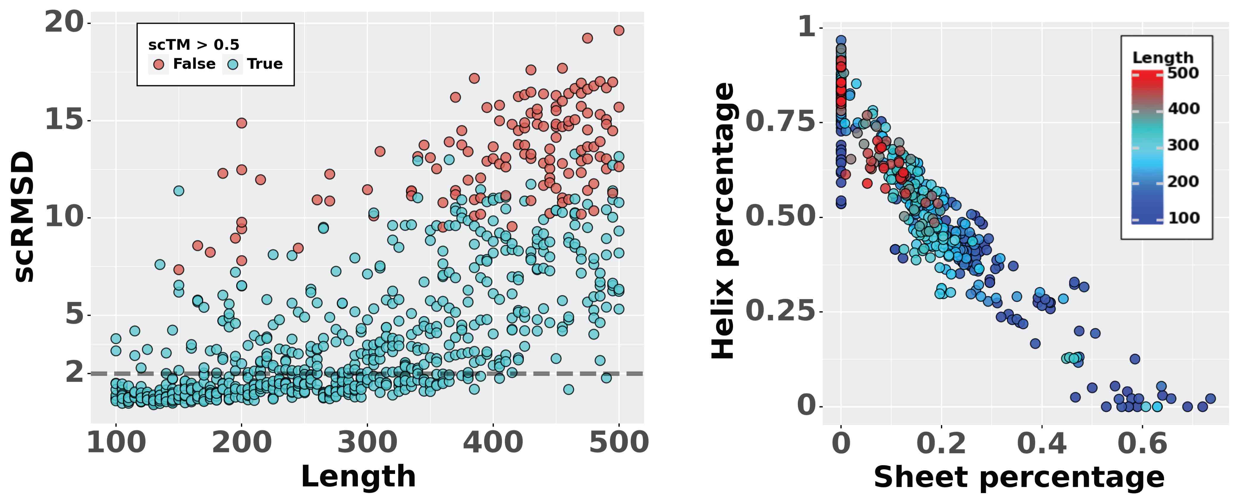
Figure 6: Additional analysis of designability across samples. Left: plot of scRMSD vs. length with color to indicate scTM$>0.5$ designability. Right: secondary structure composition of all samples across lengths.

Since RFdiffusion’s code is not released at time of writing, we reimplement the reported evaluation procedure in Watson et al. (2022) by sampling 100 backbones for each length 70, 100, 200, 300 and evaluating designability in Fig. 3A. With these samples, we additionally calculate diversity as the proportion of clusters out of 100 samples in Table 3. Interestingly, our diversity remains high despite lower noise scales in contrast to the decreased diversity reported in RFdiffusion (their diversity is reported as a bar plot across noise scales). However, $\mathrm{FrameDiff}$ designability across these lengths are lower than RFdiffusion. Exploring how to jointly improve diversity and designability will be an important research direction.

Table 3: Sample diversity compared with RFdiffusion.

	RFdiffusion			$\mathrm{FrameDiff}$
	0.0	0.5	1.0	0.1	0.5	1.0
70	0.16	0.26	0.34	0.72	0.67	0.9
100	0.26	0.35	0.65	0.59	0.52	0.81
200	0.29	0.65	0.83	0.49	0.67	0.86
300	0.17	0.67	0.91	0.62	0.52	0.8

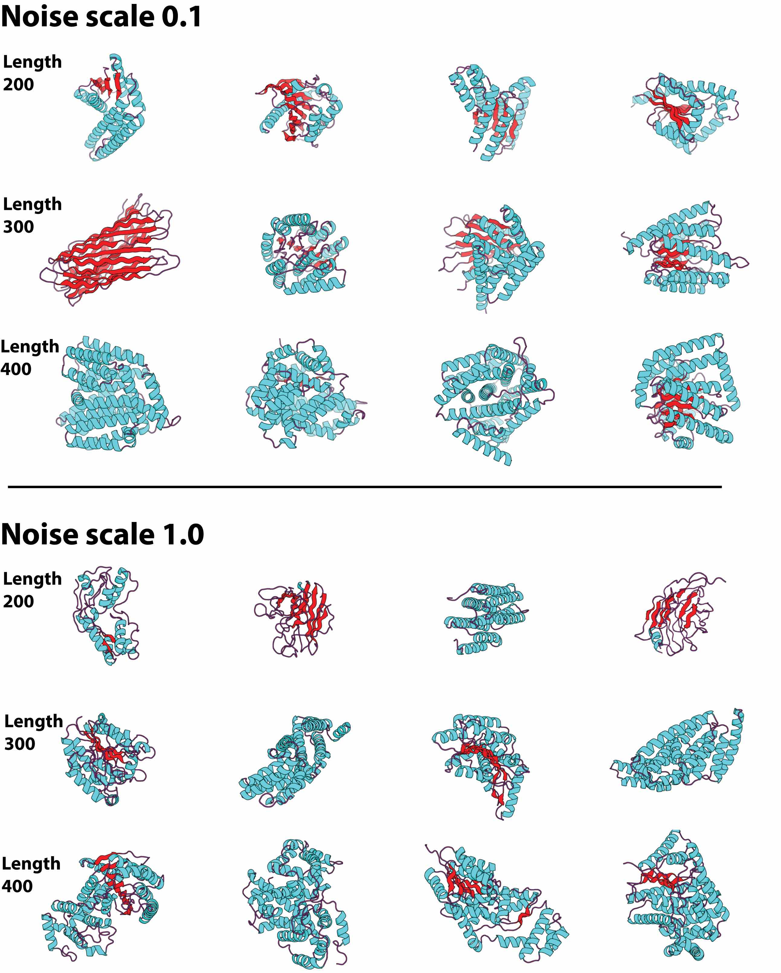
Figure 7: Visualization of samples across 4 random samples from each length group 200, 300, 40 at two different noise scales $\zeta=0.1,1.0$. Beta sheets are colored in red, alpha helices in cyan, and loops in magenta.

J.5 Comparison to FoldingDiff

In this section, we compare our results with FoldingDiff (Wu et al., 2022), a torsion angle based protein backbone diffusion model, which has publicly available code allowing for direct comparison. However, the published FoldingDiff weights are limited to generating proteins up to length 128. We re-trained FoldingDiff and performed evaluation on proteins up to length 500 on the same dataset used to train FrameDiff. To be as fair as possible, we use the evaluation code in FoldingDiff (i.e. OmegaFold for structure prediction, ProteinMPNN C-alpha only for sequence design) to evaluate FrameDiff for which we used noise scale $\zeta=1.0,N_{\mathrm{STEPS}}=500,N_{\mathrm{SEQ}}=8$. The results are in Table 4 where we see FrameDiff greatly outperforms FoldingDiff. The increase to 60% from 49% designability ( Table 1) is due to the switch from full backbone ProteinMPNN to Ca only ProteinMPNN.

Table 4: $\mathrm{FrameDiff}$ comparison to FoldingDiff.

	FoldingDiff	FrameDiff
$>0.5$ scTM ($\uparrow$)	6%	60%

References

- Ahdritz et al. (2022) Ahdritz, G., Bouatta, N., Kadyan, S., Xia, Q., Gerecke, W., O’Donnell, T. J., Berenberg, D., Fisk, I., Zanichelli, N., Zhang, B., et al. OpenFold: Retraining AlphaFold2 yields new insights into its learning mechanisms and capacity for generalization. bioRxiv, 2022.
- Albergo et al. (2021) Albergo, M. S., Boyda, D., Hackett, D. C., Kanwar, G., Cranmer, K., Racanière, S., Rezende, D. J., and Shanahan, P. E. Introduction to normalizing flows for lattice field theory. arXiv preprint arXiv:2101.08176, 2021.
- Anand & Achim (2022) Anand, N. and Achim, T. Protein structure and sequence generation with equivariant denoising diffusion probabilistic models. arXiv preprint arXiv:2205.15019, 2022.
- Arunachalam et al. (2021) Arunachalam, P. S., Walls, A. C., Golden, N., Atyeo, C., Fischinger, S., Li, C., Aye, P., Navarro, M. J., Lai, L., Edara, V. V., et al. Adjuvanting a subunit COVID-19 vaccine to induce protective immunity. Nature, 594(7862):253–258, 2021.
- Ba et al. (2016) Ba, J. L., Kiros, J. R., and Hinton, G. E. Layer normalization. arXiv preprint arXiv:1607.06450, 2016.
- Barfoot et al. (2011) Barfoot, T., Forbes, J. R., and Furgale, P. T. Pose estimation using linearized rotations and quaternion algebra. Acta Astronautica, 68(1):101–112, 2011.
- Berman et al. (2000) Berman, H. M., Westbrook, J., Feng, Z., Gilliland, G., Bhat, T. N., Weissig, H., Shindyalov, I. N., and Bourne, P. E. The protein data bank. Nucleic Acids Research, 28(1):235–242, 2000.
- Carmo (1992) Carmo, M. P. a. Riemannian Geometry / Manfredo Do Carmo ; Translated by Francis Flaherty. Mathematics. Theory and Applications. Birkhäuser, 1992.
- Chen et al. (2023) Chen, T., Zhang, R., and Hinton, G. Analog bits: Generating discrete data using diffusion models with self-conditioning. International Conference on Learning Representations (ICLR), 2023.
- Corso et al. (2023) Corso, G., Stärk, H., Jing, B., Barzilay, R., and Jaakkola, T. Diffdock: Diffusion steps, twists, and turns for molecular docking. International Conference on Learning Representations (ICLR), 2023.
- Dauparas et al. (2022) Dauparas, J., Anishchenko, I., Bennett, N., Bai, H., Ragotte, R. J., Milles, L. F., Wicky, B. I. M., Courbet, A., de Haas, R. J., Bethel, N., Leung, P. J. Y., Huddy, T. F., Pellock, S., Tischer, D., Chan, F., Koepnick, B., Nguyen, H., Kang, A., Sankaran, B., Bera, A. K., King, N. P., and Baker, D. Robust deep learning-based protein sequence design using ProteinMPNN. Science, 378(6615):49–56, 2022.
- De Bortoli et al. (2022) De Bortoli, V., Mathieu, E., Hutchinson, M., Thornton, J., Teh, Y. W., and Doucet, A. Riemannian Score-Based Generative Modeling. In Advances in Neural Information Processing Systems, 2022.
- Ding et al. (2022) Ding, W., Nakai, K., and Gong, H. Protein design via deep learning. Briefings in Bioinformatics, 23(3):bbac102, 2022.
- Ebert & Wirth (2011) Ebert, S. and Wirth, J. Diffusive wavelets on groups and homogeneous spaces. Proceedings of the Royal Society of Edinburgh Section A: Mathematics, 141(3):497–520, 2011.
- Elesedy & Zaidi (2021) Elesedy, B. and Zaidi, S. Provably strict generalisation benefit for equivariant models. In International Conference on Machine Learning, pp. 2959–2969. PMLR, 2021.
- Engh & Huber (2012) Engh, R. and Huber, R. Structure quality and target parameters. International Tables for Crystallography, 2012.
- Faraut (2008) Faraut, J. Analysis on Lie Groups: An Introduction. Cambridge Studies in Advanced Mathematics. Cambridge University Press, 2008.
- Fegan (1983) Fegan, H. The fundamental solution of the heat equation on a compact Lie group. Journal of Differential Geometry, 18(4):659–668, 1983.
- Fey & Lenssen (2019) Fey, M. and Lenssen, J. E. Fast graph representation learning with PyTorch Geometric. In ICLR Workshop on Representation Learning on Graphs and Manifolds, 2019.
- Folland (2016) Folland, G. B. A Course in Abstract Harmonic Analysis, volume 29. CRC press, 2016.
- Hall (2015) Hall, B. C. Lie Groups, Lie Algebras, and Representations, volume 222 of Graduate Texts in Mathematics. Springer International Publishing, 2015.
- Harris et al. (1991) Harris, W., Fulton, W., and Harris, J. Representation Theory: A First Course. Graduate Texts in Mathematics. Springer New York, 1991.
- Herbert & Sternberg (2008) Herbert, A. and Sternberg, M. MaxCluster: a tool for protein structure comparison and clustering. 2008.
- Ho et al. (2020) Ho, J., Jain, A., and Abbeel, P. Denoising diffusion probabilistic models. In Advances in Neural Information Processing Systems, 2020.
- Hsu (2002) Hsu, E. P. Stochastic Analysis on Manifolds. Number 38. American Mathematical Soc., 2002.
- Huang et al. (2021) Huang, C.-W., Lim, J. H., and Courville, A. C. A variational perspective on diffusion-based generative models and score matching. Advances in Neural Information Processing Systems, 2021.
- Huang et al. (2022) Huang, C.-W., Aghajohari, M., Bose, A. J., Panangaden, P., and Courville, A. Riemannian diffusion models. In Advances in Neural Information Processing Systems, 2022.
- Huang et al. (2016) Huang, P.-S., Boyken, S. E., and Baker, D. The coming of age of de novo protein design. Nature, 537(7620):320–327, 2016.
- Ikeda & Watanabe (2014) Ikeda, N. and Watanabe, S. Stochastic Differential Equations and Diffusion Processes. Elsevier, 2014.
- Ingraham et al. (2022) Ingraham, J., Baranov, M., Costello, Z., Frappier, V., Ismail, A., Tie, S., Wang, W., Xue, V., Obermeyer, F., Beam, A., and Grigoryan, G. Illuminating protein space with a programmable generative model. bioRxiv, 2022.
- (31) Jing, B., Corso, G., Chang, J., Barzilay, R., and Jaakkola, T. S. Torsional diffusion for molecular conformer generation. In Advances in Neural Information Processing Systems.
- Jumper et al. (2021) Jumper, J. M., Evans, R., Pritzel, A., Green, T., Figurnov, M., Ronneberger, O., Tunyasuvunakool, K., Bates, R., Zídek, A., Potapenko, A., Bridgland, A., Meyer, C., Kohl, S. A. A., Ballard, A., Cowie, A., Romera-Paredes, B., Nikolov, S., Jain, R., Adler, J., Back, T., Petersen, S., Reiman, D. A., Clancy, E., Zielinski, M., Steinegger, M., Pacholska, M., Berghammer, T., Bodenstein, S., Silver, D., Vinyals, O., Senior, A. W., Kavukcuoglu, K., Kohli, P., and Hassabis, D. Highly accurate protein structure prediction with AlphaFold. Nature, 596(7873):583 – 589, 2021.
- Kabsch & Sander (1983) Kabsch, W. and Sander, C. Dictionary of protein secondary structure: pattern recognition of hydrogen-bonded and geometrical features. Biopolymers: Original Research on Biomolecules, 22(12):2577–2637, 1983.
- (34) Karras, T., Aittala, M., Aila, T., and Laine, S. Elucidating the design space of diffusion-based generative models. In Advances in Neural Information Processing Systems.
- Kingma & Ba (2014) Kingma, D. P. and Ba, J. Adam: A method for stochastic optimization. arXiv preprint arXiv:1412.6980, 2014.
- Knapp & Knapp (1996) Knapp, A. W. and Knapp, A. Lie Groups: Beyond An Introduction, volume 140. Springer, 1996.
- Köhler et al. (2020) Köhler, J., Klein, L., and Noé, F. Equivariant flows: exact likelihood generative learning for symmetric densities. In International Conference on Machine Learning, 2020.
- Lane (2023) Lane, T. J. Protein structure prediction has reached the single-structure frontier. Nature Methods, pp. 1–4, January 2023.
- Leach et al. (2022) Leach, A., Schmon, S. M., Degiacomi, M. T., and Willcocks, C. G. Denoising diffusion probabilistic models on so (3) for rotational alignment. In ICLR 2022 Workshop on Geometrical and Topological Representation Learning, 2022.
- Lee (2013) Lee, J. M. Smooth manifolds. In Introduction to Smooth Manifolds, pp. 1–31. Springer, 2013.
- Lin et al. (2023) Lin, Z., Akin, H., Rao, R., Hie, B., Zhu, Z., Lu, W., Smetanin, N., Verkuil, R., Kabeli, O., Shmueli, Y., dos Santos Costa, A., Fazel-Zarandi, M., Sercu, T., Candido, S., and Rives, A. Evolutionary-scale prediction of atomic-level protein structure with a language model. Science, 379(6637):1123–1130, 2023. doi: 10.1126/science.ade2574. URL https://www.science.org/doi/abs/10.1126/science.ade2574.
- Luo et al. (2022) Luo, S., Su, Y., Peng, X., Wang, S., Peng, J., and Ma, J. Antigen-specific antibody design and optimization with diffusion-based generative models for protein structures. In Koyejo, S., Mohamed, S., Agarwal, A., Belgrave, D., Cho, K., and Oh, A. (eds.), Advances in Neural Information Processing Systems, 2022.
- (43) Murray, R., Li, Z., Sastry, S., and Sastry, S. A Mathematical Introduction to Robotic Manipulation. Taylor & Francis.
- Nikolayev & Savyolov (1970) Nikolayev, D. I. and Savyolov, T. I. Normal distribution on the rotation group SO(3). Textures and Microstructures, 29, 1970.
- Pollard (2002) Pollard, D. A User’s Guide to Measure Theoretic Probability. Cambridge University Press, 2002.
- Qiao et al. (2022) Qiao, Z., Nie, W., Vahdat, A., Miller III, T. F., and Anandkumar, A. Dynamic-backbone protein-ligand structure prediction with multiscale generative diffusion models. arXiv preprint arXiv:2209.15171, 2022.
- Quijano-Rubio et al. (2020) Quijano-Rubio, A., Ulge, U. Y., Walkey, C. D., and Silva, D.-A. The advent of de novo proteins for cancer immunotherapy. Current Opinion in Chemical Biology, 56:119–128, 2020. Next Generation Therapeutics.
- Sola et al. (2018) Sola, J., Deray, J., and Atchuthan, D. A micro Lie theory for state estimation in robotics. arXiv preprint arXiv:1812.01537, 2018.
- Song et al. (2021) Song, Y., Sohl-Dickstein, J., Kingma, D. P., Kumar, A., Ermon, S., and Poole, B. Score-based generative modeling through stochastic differential equations. In International Conference on Learning Representations, 2021.
- Trippe et al. (2023) Trippe, B. L., Yim, J., Tischer, D., Broderick, T., Baker, D., Barzilay, R., and Jaakkola, T. Diffusion probabilistic modeling of protein backbones in 3d for the motif-scaffolding problem. International Conference on Learning Representations (ICLR), 2023.
- Urain et al. (2022) Urain, J., Funk, N., Chalvatzaki, G., and Peters, J. Se (3)-diffusionfields: Learning cost functions for joint grasp and motion optimization through diffusion. arXiv preprint arXiv:2209.03855, 2022.
- van Kempen et al. (2023) van Kempen, M., Kim, S. S., Tumescheit, C., Mirdita, M., Lee, J., Gilchrist, C. L., Söding, J., and Steinegger, M. Fast and accurate protein structure search with foldseek. Nature Biotechnology, pp. 1–4, 2023.
- Vaswani et al. (2017) Vaswani, A., Shazeer, N., Parmar, N., Uszkoreit, J., Jones, L., Gomez, A. N., Kaiser, Ł., and Polosukhin, I. Attention is all you need. In Advances in Neural Information Processing Systems, 2017.
- Watson et al. (2022) Watson, J. L., Juergens, D., Bennett, N. R., Trippe, B. L., Yim, J., Eisenach, H. E., Ahern, W., Borst, A. J., Ragotte, R. J., Milles, L. F., Wicky, B. I. M., Hanikel, N., Pellock, S. J., Courbet, A., Sheffler, W., Wang, J., Venkatesh, P., Sappington, I., Torres, S. V., Lauko, A., De Bortoli, V., Mathieu, E., Barzilay, R., Jaakkola, T. S., DiMaio, F., Baek, M., and Baker, D. Broadly applicable and accurate protein design by integrating structure prediction networks and diffusion generative models. bioRxiv, 2022.
- Weyl & Peter (1927) Weyl, H. and Peter, P. Die Vollständigkeit der primitiven Darstellungen einer geschlossenen kontinuierlichen Gruppe. 97:737–755, 1927.
- Wu et al. (2022) Wu, K. E., Yang, K. K., Berg, R. v. d., Zou, J. Y., Lu, A. X., and Amini, A. P. Protein structure generation via folding diffusion. arXiv preprint arXiv:2209.15611, 2022.
- Xu et al. (2022) Xu, M., Yu, L., Song, Y., Shi, C., Ermon, S., and Tang, J. GeoDiff: A Geometric Diffusion Model for Molecular Conformation Generation. In International Conference on Learning Representations, 2022.