Statistical properties of the two dimensional Feshbach–Villars oscillator (FVO) in the Rotating Cosmic String space-time

Abstract

This paper is concerned with an investigation of the quantum mechanical dynamics of massive, spinless relativistic Klein-Gordon particle in the space-time generated by a rotating cosmic string. The equations of motion are found by the use of the first-order Feshbach-Villars formulation of the Klein-Gordon equation. The wave-functions and the associated energies were deduced ( both in the free and in the interaction case). Following that, the partition function was approximated using Zeta function representation. Moreover, by considering the energy spectrum of the system in question, the thermal properties are presented. We examine the behavior of these properties as a function of the physical parameters of the model such as rotation, curvature, and quantum numbers. Therefore, the impact of the topological defect on the quantum system under investigation is discussed.

I Introduction

It is of general interest to understand the influence of the gravitational field on the dynamics of quantum mechanical systems. Einstein’s theory of general relativity (GR) (key-1, ), on the one hand, provides a persuasive description of gravity as a geometric property of space-time. In particular, it demonstrates that the classical gravitational field is a manifestation of the curvature of space-time. It has, for example, successfully predicted the existence of gravitational waves (key-2, ) and black holes(key-3, ). Quantum mechanics (QM), on the other hand, is the framework for describing the behavior of particles in the microscopic scale (key-4, ). It is an extremely successful theory (typically quantum field theory) in explaining how the tiny particles interact and how three of the four fundamental forces of nature: the weak, strong, and electromagnetic interactions are emerged (key-5, ). However, the attempts to have a unified theory which can reconcile general relativity and quantum mechanics i.e. a theory of quantum gravity, is still suffering from several obstacles and technical issues that cannot being encountered, at least until the recent time (key-6, ; key-7, ) .

One basic method for formulating a theory in which the interface between gravity and relativistic quantum mechanics arises, is by generalizing the aspects of the relativistic dynamics of particles in flat Minkowski space to an arbitrary curved background geometry (key-8, ; key-9, ) , and therefore one can extend this formulation to establish a broad picture on how the gravitational field affects on the relativistic particles at quantum level. In this way, it is possible to adapt the approach to deal with different models where the notion of curvature appears, and hence incorporating more predictions on the values of macroscopic observables which are required to make relevant experimental verification of certain phenomenological consequences, specifically in astrophysics and cosmology. In addition, understanding the thermodynamic behavior of relativistic particles where gravitational effects have to be taken into account (key-10, ; key-11, ; key-12, ), and analyzing the associated features i.e, the fundamental statistical quantities, would offer the possibility of obtaining useful and essential results in the context of describing the quantum behavior of gravity.

Over the past few decades, topological defects ( domain walls, cosmic strings, monopoles, and textures ) have been tackled intensively as a subject of research and still remain one of the most active fields in condensed matter physics, cosmology, astrophysics and elementary particle models. It is believed that these structures raised as a consequence of the Kibble mechanism (key-13, ; key-14, ; key-15, ) where the defects are formed in symmetry-breaking phase transitions during the cooling of the early universe (key-16, ; key-17, ). The particular defect we are interested in, is cosmic strings (for more reviews we refer the reader to (key-18, )). These objects ( static or rotating) can produce observable effects. For example, they provide a promising scheme for seeding galaxy formation and the gravitational lensing effects. Moreover, by studying cosmic strings and their properties, we can learn much more about particle physics at very high energies in different scenarios. In addition, the possibility that cosmic strings could behave like superconducting wires has been raised with intriguing consequences in modern physics.

It has been known for many years now that the harmonic oscillator (HO) is considered as an essential tool in many disciplines of theoretical physics (key-19, ). It is a well studied exactly solvable model which can be used to analyze various complex problems in the framework of quantum mechanics (key-20, ). Furthermore the relativistic generalization of the quantum harmonic oscillator yields an effective model in explaining very diverse aspects of molecular, atomic and nuclear interactions. Indeed, the feature of having a complete set of exact analytical solutions when dealing with such model can give rise to significantly different explanations of many mathematical and physical phenomena, and hence related applications can be achieved via the underlying formulation.

It is now accepted that the behavior of several relativistic quantum systems depends crucially on the so-called Dirac oscillator (DO). As pointed out by Itô et al. (key-21, ) in earlier developments of spin-1/2 particle dynamics with linear trajectory. They showed that the non-relativistic limit of this system leads to the ordinary harmonic oscillator with a strong spin-orbit coupling term. Actually, according to Moshinsky and Szczepaniak (key-22, ) the above mentioned DO could be obtained from the free Dirac equation by introducing an external linear potential through a minimal substitution of the momentum operator $\hat{p}\longrightarrow\hat{p}-im\omega\beta\hat{r}$. It is interesting to point out that besides the theoretical focus on studying the DO, valuable insights can be obtained by considering the physical interpretation which is certainly essential in understanding many relevant applications.

Inspired by DO, an analogous formalism was introduced for the case of bosonic particles and hence it was named a Klein-Gordon oscillator (KGO) (key-23, ; key-24, ). The covariant form of this model in curved space-time and within different configurations, has recently been an active field of investigation by several authors. There are numerous contributions on the subject of the relativistic quantum motions of scalar and vector particles under gravitational effects produced by different curved space-time geometries, for example, the problem of the interaction between KGO coupled harmonically with topological defects in Kaluza-Klein theory is studied in Ref. (key-25, ). The relativistic quantum dynamics of spin-0 particles in a rotating cosmic string space-time with a scalar and vector potentials of Coulomb-type has been studied in Ref. (key-26, ). Furthermore, rotating effects on the scalar field in the cosmic string space-time, in the space-time with space-like dislocation and in the space-time with a spiral dislocation have been investigated in Ref. (key-27, ). Recently, the authors of Ref. (key-28, ) have analyzed the KGO in a cosmic string space-time and studied the effects stemming from the rotating frame and non-commutativity in momentum space. In addition, the KGO subjected to a magnetic quantum flux in the presence of a Cornell-type scalar and Coulomb-type vector potentials in a rotating cosmic string space-time have been examined in Ref. (key-29, ).

Attempts to investigate the relativistic spin-0, spin-1 bosons and spin-1/2 fermions wave functions and their time evolution have been pursued by various authors (key-30, ; key-31, ; key-32, ) making use of the Hamiltonian form i.e, having Schrodinger’s equations. The so-called Feshbach-Villars (FV) equations (key-33, ) are of particular interest in this respect. These equations were initially constructed in the purpose of permitting a relativistic single particle interpretation of the second order KG equation. For the later case, FV equations originate from splitting the KG wave function into two components in order to obtain an equation with first order time derivative. In recent decades, a number of papers have been produced with the aim of exploring the relativistic dynamical properties of single particles and solving their wave equations by adopting the FV scheme (e.g, Refs. (key-34, ; key-35, ; key-36, ; key-37, ; key-38, ; key-39, ; key-40, ) and other related references cited therein).

In a quest to map out a description of the dynamics of spinless, massive bosons in a space-time with a topological defect, namely the cosmic string geometry, we employ the methods of the FV transformation to derive FV equations of motion in a static and rotating cosmic string backgrounds. The main purpose of this paper is , firstly to solve the derived FV equations and obtain the associated spectra, and secondly, to investigate the thermodynamic properties of these systems and understand how the geometry of the space-time affects on the observable quantities.

The structure of this paper is as follows. In the next section we derive the FV equations for scalar boson in Minkowski and static Cosmic string space-time considering both the free and the interaction case. We introduce the KG oscillator in a Hamiltonian form, then we solve the obtained equations to deduce the eigenstates and the energy levels. In section 3 we furthermore construct the previous equations in the case where the geometry of the cosmic string is characterized by a rotation, the same procedure of Section 2 is used in this section. In section 4 we study the statistical properties of the system in question and we discuss the influence of the topological defect on these quantities. We give our conclusions in section 5. Throughout the paper, we will always use natural units $\hbar=c=G=K_{B}=1$ , and our metric convention is $(+,-,-,-$).

II The FV Representation of Spin-0 Particle in Minkowski Space-time

II.1 Klein-Gordon Equation in Schrödinger Form

In this section, we deal with the relativistic quantum description of spin-0 particle propagating in Minkowski space-time with the metric tensor $\eta_{\mu\nu}=\text{diag}\left(1,-1,-1,-1\right)$. For a scalar massive particle $\Phi$ with mass $m>0$, the standard covariant KG equation reads (key-41, ; key-42, )

$$\left(\eta^{\mu\nu}D_{\mu}D_{\nu}+m^{2}\right)\Phi(x,t)=0,$$ (1)

where $D_{\mu}=i\left(p_{\mu}-eA_{\mu}\right)$ denotes the minimally coupled covariant derivative. $p_{\mu}=\left(E,-p_{i}\right)$ is the canonical four momentum and $A_{\mu}=\left(A_{0},-A_{i}\right)$ is the electromagnetic four potential, respectively. $e$ is the magnitude of the particle charge.

At this place, it is worth emphasizing that Eq. ((1)) can be rewritten in a Hamiltonian form with the time first derivative i.e, a Schrodinger’s equation

$$\mathcal{H}\Phi\left(x,t\right)=i\,\frac{\partial}{\partial t}\Phi(x,t).$$ (2)

The Hamiltonian $\mathcal{H}$ can be defined by the use of the FV linearization procedure i.e, transforming Eq. (1) to a first order in time differential equation. We introduce the two component wave function (key-43, ; key-44, ),

$$\Phi(x,t)=\left(\begin{array}[]{c}\phi_{1}(x,t)\\ \phi_{2}(x,t)\end{array}\right)=\frac{1}{\sqrt{2}}\left(\begin{array}[]{c}1+\frac{i}{m}\mathcal{D}\\ 1-\frac{i}{m}\mathcal{D}\end{array}\right)\psi(x,t),$$ (3)

here $\psi(x,t)$ obeys the KG wave equation, and we have defined $\mathcal{D}$ such that

$$\mathcal{D}=\frac{\partial}{\partial t}+ieA_{0}(x),$$ (4)

the above transformation ((3)) consists in introducing wave functions satisfying the conditions

$$\psi=\phi_{1}+\phi_{2},\qquad i\mathcal{D}\psi=m\left(\phi_{1}-\phi_{2}\right).$$ (5)

For our subsequent review, it is convenient to write

$$\phi_{1} =\frac{1}{2m}\left[m+i\frac{\partial}{\partial t}-eA_{0}\right]\psi$$ (6)

$$\phi_{2} =\frac{1}{2m}\left[m-i\frac{\partial}{\partial t}+eA_{0}\right]\psi,$$

Equivalently, Eq. ((1)) becomes

$$\left[i\frac{\partial}{\partial t}-eA_{0}\right]\left(\phi_{1}+\phi_{2}\right) =m\left(\phi_{1}-\phi_{2}\right)$$ (7)

$$\left[i\frac{\partial}{\partial t}-eA_{0}\right]\left(\phi_{1}-\phi_{2}\right) =\left[\frac{\left(p_{i}-eA_{i}\right)^{2}}{m}+m\right]\left(\phi_{1}+\phi_{2}\right),$$

Addition and subtraction of these two equations lead to the system of coupled differential equations of first order in time,

$$\frac{\left(p_{i}-eA_{i}\right)^{2}}{2m}\left(\phi_{1}+\phi_{2}\right)+\left(m+eA_{0}\right)\phi_{1} =i\frac{\partial\phi_{1}}{\partial t}$$ (8)

$$\frac{-\left(p_{i}-eA_{i}\right)^{2}}{2m}\left(\phi_{1}+\phi_{2}\right)-\left(m-eA_{0}\right)\phi_{2} =i\frac{\partial\phi_{2}}{\partial t},$$

Using Eqs. ((8)), the FV Hamiltonian of a scalar particle in the presence of the electromagnetic interaction may be written as

$$\mathcal{H}_{KG}=\left(\tau_{z}+i\tau_{y}\right)\frac{\left(p_{i}-eA_{i}\right)^{2}}{2m}+m\tau_{z}+eA_{0}(x),$$ (9)

where $\tau_{i}\,\left(i=x,y,z\right)$ are the conventional $2\times 2$ Pauli matrices given by

$$\tau_{x}=\left(\begin{array}[]{cc}0&1\\ 1&0\end{array}\right),\quad\tau_{y}=\left(\begin{array}[]{cc}0&-i\\ i&0\end{array}\right),\quad\tau_{z}=\left(\begin{array}[]{cc}1&0\\ 0&-1\end{array}\right).$$ (10)

It is noteworthy that the Hamiltonian ((9)) fulfills the generalized hermicity condition ,

$$\mathcal{H}_{KG}=\tau_{z}\mathcal{H}_{KG}^{\dagger}\tau_{z},\qquad\mathcal{H}_{KG}^{\dagger}=\tau_{z}\mathcal{H}_{KG}\tau_{z}.$$ (11)

For the free particle propagation i.e, no interaction is considered $\left(A_{\mu}=0\right),$ the one dimensional FV Hamiltonian simplifies to

$$\mathcal{H}_{0}=\left(\tau_{z}+i\tau_{y}\right)\frac{p_{x}^{2}}{2m}+m\tau_{z},$$ (12)

The solutions to the free Hamiltonian (which is independent of time) are just stationary states. Assuming a solution of the form (key-36, ),

$$\Phi\left(x,t\right)=\Phi\left(x\right)e^{-iEt}=\left(\begin{array}[]{c}\phi_{1}\left(x\right)\\ \phi_{2}\left(x\right)\end{array}\right)e^{-iEt},$$ (13)

with $E$ being the energy of the system. Thus, Eq. ((2)) can then be written as

$$\mathcal{H}_{0}\Phi\left(x\right)=E\Phi\left(x\right),$$ (14)

which is the one-dimensional FV equation of the free relativistic spin-0 particle and it is carried out with the aim of having an alternative Schrodinger’s to KG equation. In what follows, the above method will be used to find the solutions of wave equations in curved space-time, namely, the cosmic string.

II.2 KGO in Schrödinger Form

For the next discussion, it is preferable to analyze the KGO in Minkowski space-time exploiting the method described previously. In order to examine the KGO in the FV representation, we start with the minimal substitution $p_{\mu}\longrightarrow p_{\mu}+im\omega x_{\mu}$ of the momentum operator (key-46, ). Here $\omega$ is the oscillation frequency and $x_{\mu}=(0,x,0,0)$ . Thus, by generalizing the momentum operator, the one dimensional FV Hamiltonian ((12)) becomes

$$\mathcal{H}_{KGO}=\frac{1}{2m}\left(\tau_{z}+i\tau_{y}\right)\left(P_{x}-im\omega x\right)\left(P_{x}+im\omega x\right)+m\tau_{z},$$ (15)

In this way, one obtains the Schrödinger formulation of KGO in one dimension by substituting the Ansatz ((13)) into Eq. ((14)) by means of Eq. ((15)),

$$\frac{1}{2m}\left[\frac{d^{2}}{dx^{2}}-m^{2}\omega^{2}x^{2}+m\omega\right]\left(\phi_{1}+\phi_{2}\right)+m\phi_{1} =E\phi_{1}$$ (16)

$$-\frac{1}{2m}\left[\frac{d^{2}}{dx^{2}}-m^{2}\omega^{2}x^{2}+m\omega\right]\left(\phi_{1}+\phi_{2}\right)-m\phi_{2} =E\phi_{2},$$

after performing a calculation similar to the one was done in the previous KG equation case, then it follows that

$$\left[\frac{d^{2}}{dx^{2}}-m^{2}\omega^{2}x^{2}+\left(E^{2}-m^{2}+m\omega\right)\right]\psi\left(x\right)=0,$$ (17)

or,

$$\left[\frac{d^{2}}{dx^{2}}-\lambda_{1}x^{2}+\lambda_{2}\right]\psi\left(x\right)=0$$ (18)

where we have set,

$$\lambda_{1}=m^{2}\omega^{2},\qquad\lambda_{2}=E^{2}-m^{2}+m\omega.$$ (19)

Eq. ((18)) is a second order differential equation for the field $\psi$ describing the KGO dynamics in one dimensional Minkowski space-time. The solution of the above equation can be found in literature, and a quantization condition of the energy is followed from that solution, providing

$$\frac{E^{2}-m^{2}+m\omega}{2m}=\left(n+\frac{1}{2}\right)\omega,\qquad n=0,1,2,\cdots.$$ (20)

After arranging and simplifying the condition ((20)), we find the following expression of the energy spectrum

$$E=\pm\sqrt{2m\omega n+m^{2}},$$ (21)

Eq.((21)) presents the relativistic energy spectrum of KGO in Minkowski space-time.

III The FV Representation of Spin-0 Particle in Cosmic String Space-time

The purpose of this section is to study the KGO in the background geometry of a cosmic string with the use of the FV scheme. It is well known that the generally covariant relativistic wave equations of a scalar particle in a Riemannian space-time defined by the metric tensor $g_{\mu\nu}$ , can be obtained by reformulating the KG equation such that ( see, e.g, the textbooks (key-8, ; key-9, ) )

$$\left(\square+m^{2}-\xi R\right)\Phi(x,t)=0,$$ (22)

where $\square$ is the Laplace-Beltrami operator given by

$$\square=g^{\mu\nu}D_{\mu}D_{\nu}=\frac{1}{\sqrt{-g}}\partial_{\mu}\left(\sqrt{-g}g^{\mu\nu}\partial_{\nu}\right),$$ (23)

$\xi$ is a real dimensionless coupling constant and $R$ is the Ricci scalar curvature defined by $R=g^{\mu\nu}R_{\mu\nu}$ where $R_{\mu\nu}$ is the Ricci curvature tensor. $g^{\mu\nu}$ is the inverse metric tensor and $g=\det\left(g^{\mu\nu}\right)$.

We now would like to study the quantum dynamics of spin-0 particles in the space-time induced by a (2+1)-dimensional static cosmic string and set up the corresponding FV formulation.

III.1 FV formulation of KGO in static cosmic string space-time

Before we study the KGO in the Hamiltonian representation, let us first derive the KG wave equation for the free relativistic scalar particle propagating in the cosmic string space-time that is assumed to be static and cylindrical symmetric.

The general expression for a (3+1)-dimensional cosmic string metric is defined by the line element (key-47, ; key-48, )

$$ds^{2} =g_{\mu\nu}dx^{\mu}dx^{\nu}$$

$$=dt^{2}-dr^{2}-\alpha^{2}r^{2}d\varphi^{2}-dz,$$ (24)

in cylindrical coordinates . Here $-\infty\leq t\leq+\infty$, $r\geq 0$, $0\leq\varphi\leq 2\pi$, $-\infty\leq z\leq+\infty,$ and $\alpha\in[0,1[\>$ is the angular parameter which determines the angular deficit $\delta\varphi=2\pi(1-\alpha)$, and it is related to the linear mass density $\mu$ of the string by $\alpha=1-4\mu$.

For the sake of simplicity in treating our quantum mechanical problem, let us work in a lower dimensional space in which $z=\text{cont}$, and because there is no structure in $z$-direction, we can suppress it (key-49, ; key-50, ). Thus, the metric of a static cosmic string with cylindrical symmetry has a $(2+1)$-dimensional form

$$ds^{2}=dt^{2}-dr^{2}-\alpha^{2}r^{2}d\varphi^{2}$$ (25)

where the components of the metric and the inverse metric tensors are, respectively,

$$g_{\mu\nu}=\left(\begin{array}[]{ccc}1&0&0\\ 0&-1&0\\ 0&0&-\left(\alpha r\right)^{2}\end{array}\right),\quad g^{\mu\nu}=\left(\begin{array}[]{ccc}1&0&0\\ 0&-1&0\\ 0&0&\frac{-1}{\left(\alpha r\right)^{2}}\end{array}\right)$$ (26)

Its is worthy to mention that the subject of spinless massive particles in the geometry generated by a static cosmic string background has been discussed in several papers ( see, e.g, (key-25, ; key-51, ))

In what follows, we shall adopt the procedure presented in Refs. (key-52, ; key-53, ) to derive the FV form of KG wave equation in curved manifolds. We use the generalized Feshbach–Villars transformation (GFVT) which is appropriate for describing both massive and massless particles. In the GFVT, the components of the wave function $\Phi$ are given by (key-52, )

$$\psi=\phi_{1}+\phi_{2},\qquad i\tilde{\mathcal{D}}\psi=\mathcal{N}\left(\phi_{1}-\phi_{2}\right),$$ (27)

where $\mathcal{N}$ is an arbitrary nonzero real parameter, and we have defined $\tilde{\mathcal{D}}=\frac{\partial}{\partial t}+\mathcal{Y},$ with

$$\mathcal{Y}=\frac{1}{2g^{00}\sqrt{-g}}\left\{\partial_{i},\sqrt{-g}g^{0i}\right\},$$ (28)

The curly bracket in Eq. ((28)) denotes the anti-commutator. For the above mentioned transformation, the Hamiltonian reads

$$\mathcal{H}_{GFVT}=\tau_{z}\left(\frac{\mathcal{N}^{2}+\mathcal{T}}{2\mathcal{N}}\right)+i\tau_{y}\left(\frac{-\mathcal{N}^{2}+\mathcal{T}}{2\mathcal{N}}\right)-i\mathcal{Y},$$ (29)

with

$$\mathcal{T}=\frac{1}{g^{00}\sqrt{-g}}\partial_{i}\sqrt{-g}g^{ij}\partial_{j}+\frac{m^{2}-\xi R}{g^{00}}-\mathcal{Y}^{2},$$ (30)

here and below $(i,j=1,2,3)$. We note that for $\mathcal{N}=m$, the original FV transformations are satisfied.

Now, considering the metric (25), it is easy to find that $R=0$, in other words, the space-time is locally flat (there is no local gravity), and hence the coupling term is vanishing.

A straightforward calculation leads to $\mathcal{Y}=0,$ then we obtain

$$\mathcal{T}=-\frac{d^{2}}{dr^{2}}-\frac{1}{r}\frac{d}{dr}-\frac{1}{\alpha^{2}r^{2}}\frac{d^{2}}{d\varphi^{2}}+m^{2},$$ (31)

Using these results to find the Hamiltonian (29), then because of the time and angular independence in the metric (25), one can assume a solution of the form ,

$$\Phi(t,r,\varphi)=\Phi(r)e^{-i\left(Et-j\varphi\right)},$$ (32)

where $j=0,\pm 1,\pm 2,..$ are the eigenvalues of the $z$component of the angular momentum operator. Therefore, it follows that the KG equation (22) may be written equivalently to the following two coupled equations

$$\left(\mathcal{N}^{2}+\mathcal{T}\right)\phi_{1}+\left(-\mathcal{N}^{2}+\mathcal{T}\right)\phi_{2} =2\mathcal{N}E\phi_{1}$$

$$-\left(\mathcal{N}^{2}+\mathcal{T}\right)\phi_{2}-\left(-\mathcal{N}^{2}+\mathcal{T}\right)\phi_{1} =2\mathcal{N}E\phi_{2},$$ (33)

The sum and the difference of the two last equations give a second order differential equation for the field $\psi$. Thus, the radial equation is written as follows

$$\left[\frac{d^{2}}{dr^{2}}+\frac{1}{r}\frac{d}{dr}-\frac{\zeta^{2}}{r^{2}}+\kappa\right]\psi\left(r\right)=0,$$ (34)

where we have set

$$\zeta=\frac{j}{\alpha},\qquad\kappa=\sqrt{E^{2}-m^{2}}.$$ (35)

We can observe that Eq. ((34)) is a Bessel equation and its general solution is defined by (key-55, )

$$\psi\left(r\right)=A\,J_{|\zeta|}\left(\kappa r\right)+B\,Y_{|\zeta|}\left(\kappa r\right),$$ (36)

where $J_{|\zeta|}\left(\kappa r\right)$ and $Y_{|\zeta|}\left(\kappa r\right)$ are the Bessel functions of order $\zeta$ and of the first and the second kind, respectively. Here $A$ and $B$ are arbitrary constants. We notice that at the origin when $\zeta=0$, the function $J_{|\zeta|}\left(\kappa r\right)\neq 0$. However, $Y_{|\zeta|}\left(\kappa r\right)$ is always divergent at the origin. In this case, we will consider only $J_{|\zeta|}\left(\kappa r\right)$ when $\zeta\neq 0$. Hence, we write the solution to Eq. ((34)) as follows

$$\psi\left(r\right)=A\,J_{\frac{|j|}{\alpha}}\left(\sqrt{E^{2}-m^{2}}\,r\right),$$ (37)

using this solution, we can now write the complete two-components wave-function of the spinless massive KG particle in the space-time of a static cosmic string

$$\psi\left(t,r,\varphi\right)=|C|\left(\begin{array}[]{c}1+\frac{E}{\mathcal{N}}\\ 1-\frac{E}{\mathcal{N}}\end{array}\right)e^{-i\left(Et-j\varphi\right)}\,J_{\frac{|j|}{\alpha}}\left(\sqrt{E^{2}-m^{2}}\,r\right),$$ (38)

The constant $|C|$ can be obtained by the appropriate normalization condition associated with the KG equation ( e.g, see Ref. (key-56, ; key-57, )), however, it is fortunate that non determining the normalization constants throughout this manuscript does not affect the final results.

We turn now to the particular case where we want to extend the GFVT for the KGO. In general, we need to perform a substitution of the momentum operator in Eq. ((22)). Consequently, it is possible to rewrite Eq. ((30)) as follows

$$\mathcal{T}=\frac{1}{\sqrt{-g}}\left(\frac{\partial}{\partial r}-m\omega r\right)\left(-\sqrt{-g}\right)\left(\frac{\partial}{\partial r}+m\omega r\right)-\frac{1}{\alpha^{2}r^{2}}\frac{\partial^{2}}{\partial\varphi^{2}}+m^{2},$$ (39)

Similarly, a straightforward calculation based on the procedure that was carried out in the above discussion, one can obtain the following differential equation

$$\left[\frac{d^{2}}{dr^{2}}+\frac{1}{r}\frac{d}{dr}+m^{2}\omega^{2}r^{2}-\frac{\sigma^{2}}{r^{2}}+\delta\right]\psi\left(r\right)=0,$$ (40)

with

$$\sigma^{2}=\left(\frac{j}{\alpha}\right)^{2},\qquad\delta=E^{2}-m^{2}+2m\omega.$$ (41)

Eq. ((40)) is the KGO for spin-0 particle in the space-time of a static cosmic string. To obtain the solution of this equation, we first propose a transformation of the radial coordinate

$$\chi=m\omega r^{2},$$ (42)

substituting the expression for $\chi$ into Eq. ((40)), we obtain

$$\left[\frac{d^{2}}{d\chi^{2}}+\frac{1}{\chi}\frac{\partial}{d\chi}-\frac{\sigma^{2}}{4\chi^{2}}+\frac{\delta}{4m\omega\chi}-\frac{1}{4}\right]\psi\left(\chi\right)=0.$$ (43)

Now, if we study the asymptotic behavior of the wave function at the origin and infinity, and since we are looking for regular solutions, we may suppose a solution that has the form

$$\psi\left(\chi\right)=\chi^{\frac{\left|\sigma\right|}{2}}e^{-\frac{\chi}{2}}F\left(\chi\right),$$ (44)

As before, this can be substituted back into Eq. ((43)), then we have

$$\chi\frac{d^{2}F\left(\chi\right)}{d\chi^{2}}+\left(|\sigma|+1-\chi\right)\frac{dF\left(\chi\right)}{d\chi}-\left(\frac{|\sigma|}{2}-\frac{\delta}{4m\omega}+\frac{1}{2}\right)F\left(\chi\right)=0,$$ (45)

This is the confluent hyper-geometric equation (key-58, ) whose solutions are expressed in terms of the confluent hyper-geometric function type

$$F\left(\chi\right)=_{1}F_{1}\left(\frac{\left|\sigma\right|}{2}-\frac{\delta}{4m\omega}+\frac{1}{2},+1,\chi\right),$$ (46)

We should note that the solution ((46)) must be a polynomial function of degree $n$. However, taking $n\rightarrow\infty$ imposes a divergence issue. We can have a finite polynomial only if the factor of the last term in Eq. ((45)) is a negative integer, meaning,

$$\frac{\left|\sigma\right|}{2}-\frac{\delta}{4m\omega}+\frac{1}{2}=-n\qquad,n=0,1,2,\cdots.$$ (47)

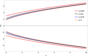
(a) $j=1.\,a=0.1,\,\omega=m=1$

Figure 1: Energy of KGO in rotating cosmic string as a function of the quantum number $n$ for different values of $\alpha$ in (a) and of $a$ in (b).

Exploiting this result, and by the insertion of the parameters ((41)), we can obtain the quantified energy spectrum of KGO in the static cosmic string space-time, hence,

$$E\left(n,\alpha,j\right)=\pm\sqrt{4m\omega n+\frac{2m\omega\left|j\right|}{\alpha}+m^{2}},$$ (48)

We can observe that the energy depends explicitly on the angular deficit $\alpha$. In other words, the curvature of the space-time which is influenced by the topological defect i.e, the cosmic string through the deficit parameter will affects on the relativistic dynamics of the scalar particle by generating a gravitational field due to the presence of the wedge angle. Fig. (1) shows the energy levels of the KGO as a function of the quantum number $n$ in a static cosmic string space characterized by a wedge parameter $\alpha$ which takes different values.

The corresponding wave function is given by

$$\psi\left(t,r,\varphi\right)=|\tilde{C}|\left(m\omega r^{2}\right)^{\frac{\left|j\right|}{2\alpha}}e^{-\frac{m\omega r^{2}}{2}}{}_{1}F_{1}\left(\frac{\left|j\right|}{2\alpha}-\frac{\delta}{4m\omega}+\frac{1}{2},\frac{|j|}{\alpha}+1,m\omega r^{2}\right),$$ (49)

Then the general eigenfunctions are expressed as

$$\psi\left(t,r,\varphi\right)=|\tilde{C}|\left(\begin{array}[]{c}1+\frac{E}{\mathcal{N}}\\ 1-\frac{E}{\mathcal{N}}\end{array}\right)\left(m\omega r^{2}\right)^{\frac{\left|j\right|}{2\alpha}}e^{-\frac{m\omega r^{2}}{2}}e^{-i\left(Et-j\varphi\right)}{}_{1}F_{1}\left(\frac{\left|j\right|}{2\alpha}-\frac{\delta}{4m\omega}+\frac{1}{2},\frac{|j|}{\alpha}+1,m\omega r^{2}\right),$$ (50)

where $|\tilde{C}|$ is the normalization constant.

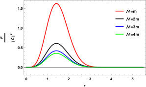
(a) $n=0,\,\alpha=0.5$

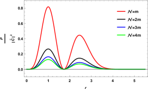
(b) $n=1,\,\alpha=0.5$

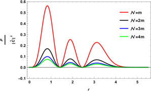
(c) $n=2,\,\alpha=0.5$

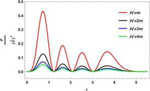
(d) $n=3,\,\alpha=0.5$

Figure 2: Plots of the density of KGO in static cosmic string as a function of the radial distance $r$ for different values of $n$ with the parameters $\alpha=0.5$ and $j=1.$

Having the complete wave-function above, we are in position to calculate the density $\rho_{{}_{KGO}}$ corresponds to the KGO given by (key-33, )

$$\rho_{{}_{KGO}}=\psi^{*}\tau_{z}\psi$$ (51)

In Fig. (2) we plot the density of KGO in static cosmic string as a function of the radial distance $r.$ Obviously, we can see that the density is affected by the choice of the variable $\mathcal{N}$.

III.2 FV formulation of KGO in rotating cosmic string space-time(41)

In this section we shall analyze the KGO in the background geometry of a rotating cosmic string in three dimensions. Similarly to the case studied in Sec. III, the equations of motion of a scalar particle can be achieved by considering the GFVT. Several authors studied the quantum dynamics of relativistic particles in the space-time of a cosmic string with rotational effects, and many models were considered in this context. For instance, in a previous paper by Mazur (key-59, ), the quantum mechanical properties of massive (or massless) particles in the gravitational field of spinning cosmic strings were discussed. He showed that the energy should be quantized in the presence of non-zero angular momentum of the string. Later, Gerbert and Jackiw (key-60, ) have presented solutions for the KG and Dirac equations in the (2+1)-dimensional space-time created by a massive point particle, with arbitrary angular momentum. In Ref. (key-61, ), the vacuum expectation value of the stress-energy tensor for a massless scalar field conformally coupled to gravitation was discussed. The authors of Ref. (key-62, ) have examined the behavior of a quantum test particle satisfying the Klein-Gordon equation in a space-time of a spinning cosmic string. Additionally, it was shown in Ref. (key-63, ) that rotating cosmic string solution of $U(1)$ scalar field theory with a cylindrical symmetric energy density can be characterized as an extrema of the field’s energy for given angular and linear momenta. Moreover, topological and geometrical phases due to gravitational field of a cosmic string that has mass and angular momentum were investigated in Ref. (key-64, ).

Recently, the subject of gravitational effects of rotating cosmic strings has attracted considerable interest in connection with the dynamics of relativistic quantum particles and their properties. For example, vacuum fluctuations for a massless scalar field around a spinning cosmic string were studied in Ref. (key-65, ) applying a re-normalization method. In like manner, vacuum polarization of a scalar field in the gravitational background of a spinning cosmic string was investigated in Ref. (key-66, ). Furthermore, the authors of Ref. (key-67, ) have analyzed the Landau levels of a spinless massive particle in the spacetime of a rotating cosmic string by means of a fully relativistic approach. Wang et al. (key-68, ) have treated the model of the KGO coupled to a uniform magnetic field in the background of the rotating cosmic string. Also, the problem of a spinless relativistic particle subjected to a uniform magnetic field in the spinning cosmic string space-time was addressed in Ref.(key-69, ). Besides, the relativistic quantum dynamics of a KG scalar field subjected to a Cornell potential in spinning cosmic string space-time was presented in Ref. (key-70, ). In addition, the relativistic scalar charged particle in a rotating cosmic string space-time with Cornell-type potential and Aharonov-Bohm effect was analyzed in Ref. (key-29, ). Other publications in which rotating cosmic strings have been considered to study the quantum properties of relativistic systems could be mentioned in this respect (e.g, (key-71, ; key-72, ; key-73, ; key-74, ; key-75, ; key-76, ; key-77, ; key-78, ) and related references therein). Aside from investigating bosonic particles in that specific space-time, in the literature one can find various discussions concerning the effects of the topology and geometry of this space-time on the quantum dynamics of fermionic particles and their behaviour ( see for instance Refs. (key-79, ; key-80, ; key-81, ; key-82, ; key-83, ; key-84, ; key-85, )).

In the next discussion, we extend the problem studied in Sec. III to a more general space-time with non-zero angular momentum. We consider a massive, relativistic spin-0 particle whose wave-function is denoted by $\Psi$ and satisfies the KG equation 22 in the space-time induced by a (2+1)-dimensional stationary rotating cosmic string which is described by the following line element (key-86, ; key-87, ; key-59, ).

$$ds^{2}=dt^{2}+2a\,dt\,d\phi-dr^{2}-\left(\alpha^{2}r^{2}-a^{2}\right)d\varphi^{2},$$ (52)

always the cylindrical coordinates $(t,r,\varphi)$ are with usual ranges, and $\alpha=1-4\mu$ is the wedge parameter with $\alpha<1.$ Here, the rotation parameter $a=4J$ has units of distance with $J$ stands for the angular momentum of the string.

The covariant and contravariant components of the metric tensor are

$$g_{\mu\nu}=\left(\begin{array}[]{ccc}1&0&a\\ 0&-1&0\\ a&0&-\left(\alpha^{2}r^{2}-a^{2}\right)\end{array}\right),\quad g^{\mu\nu}=\left(\begin{array}[]{ccc}1-\frac{a^{2}}{\alpha^{2}r^{2}}&0&\frac{a}{\alpha^{2}r^{2}}\\ 0&-1&0\\ \frac{a}{\alpha^{2}r^{2}}&0&-\frac{1}{\alpha^{2}r^{2}}\end{array}\right).$$ (53)

To study the relativistic quantum motion of a scalar boson interacting with the gravitational field of the background geometry defined by the metric 52, we need to write the generic KG equation in the curved space in question, given by

$$\left(\square+m^{2}-\xi R\right)\Psi(t,r,\varphi)=0,$$ (54)

where $\Psi$ is a two-components vector

$$\Psi(x)=\left(\begin{array}[]{c}\phi_{1}\left(x\right)\\ \phi_{2}\left(x\right)\end{array}\right),\qquad x\equiv(t,r,\varphi).$$ (55)

satisfying the condition

$$\psi=\phi_{1}+\phi_{2},\qquad i\mathcal{D}^{\prime}\psi=\mathcal{N}\left(\phi_{1}-\phi_{2}\right),$$ (56)

with $\mathcal{D}^{\prime}=\frac{\partial}{\partial t}+\mathcal{Y^{\prime}}.$

The next step is to develop the approach used in Sec III for the case of rotating cosmic strings. We adopt the GFVT to derive the equations of motion for this problem, then we solve them to obtain the wave functions and the energy spectra. Following Ref. (key-52, ; key-53, ) , the identification of the Hamiltonian leads to the idea of employing a two-components formulation of the KG type fields. In order to rewrite Eq. (54) in the Hamiltonian form, one requires to introduce new definitions for the quantities presented in Eqs. ((29)), ((30)) and ((28)). In the case under consideration, we have

$$\mathcal{H}_{GFVT}^{\prime}=\tau_{z}\left(\frac{\mathcal{N}^{2}+\mathcal{T^{\prime}}}{2\mathcal{N}}\right)+i\tau_{y}\left(\frac{-\mathcal{N}^{2}+\mathcal{T^{\prime}}}{2\mathcal{N}}\right)-i\mathcal{Y}^{\prime},$$ (57)

$$\mathcal{T}^{\prime} =\partial_{i}\frac{G^{ij}}{g^{00}}\partial_{j}+\frac{m^{2}-\xi R}{g^{00}}+\frac{1}{\mathcal{F}}\nabla_{i}\left(\sqrt{-g}G^{ij}\right)\nabla_{j}\left(\frac{1}{\mathcal{F}}\right)+\sqrt{\frac{\sqrt{-g}}{g^{00}}}G^{ij}\nabla_{i}\nabla_{j}\left(\frac{1}{\mathcal{F}}\right)+\frac{1}{4\mathcal{F}^{4}}\left[\nabla_{i}\left(\mathcal{U}^{i}\right)\right]^{2}$$

$$\qquad-\frac{1}{2\mathcal{F}^{2}}\nabla_{i}\left(\frac{g^{0i}}{g^{00}}\right)\nabla_{j}\left(\mathcal{U}^{i}\right)-\frac{g^{0i}}{2g^{00}\mathcal{F}^{2}}\nabla_{i}\nabla_{j}\left(\mathcal{U}^{i}\right),$$ (58)

$$\mathcal{Y}^{\prime}=\frac{1}{2}\left\{\partial_{i},\sqrt{-g}\frac{g^{0i}}{g^{00}}\right\},$$ (59)

where

$$G^{ij}=g^{ij}-\frac{g^{0i}g^{0j}}{g^{00}},\qquad\mathcal{F}=\sqrt{g^{00}\sqrt{-g}},\qquad\mathcal{U}^{i}=\sqrt{-g}g^{0i}.$$ (60)

It has been shown in Ref. (key-53, ) that the transformations ((57)), ((58)) and (59) with the definitions ((60)) are exact and covers any inertial and gravitational fields. It should be noted that these exact transformations ensures to obtain the block-diagonal form of the Hamiltonian $\mathcal{H}_{GFVT}$ which does not depend on the parameter $\mathcal{N}.$ For the geometry ((53)), the eigenvalues of the operator $\mathcal{Y}^{\prime}$ are given by

$$\mathcal{Y}^{\prime}\Psi\left(t,r,\varphi\right)=\frac{1}{2}\left\{\partial_{2},\sqrt{-g}\frac{g^{02}}{g^{00}}\right\}\Psi\left(t,r,\varphi\right)=\frac{g^{02}}{g^{00}}\frac{\partial}{\partial\varphi}\Psi\left(t,r,\varphi\right),$$ (61)

where the field $\Psi$ obeys the non-unitary transformation $\Psi\equiv\Phi^{\prime}=\mathcal{F}\Phi$ which permits to obtain pseudo-Hermitian Hamiltonian $\mathcal{H}_{GFVT}^{\prime}=\mathcal{F}\mathcal{H}_{GFVT}^{\prime}\mathcal{F}^{-1},$ $\mathcal{H}_{GFVT}^{\prime}=\tau_{z}\left(\mathcal{H}_{GFVT}^{\prime}\right)^{\dagger}\tau_{z}.$

After some mathematical calculations, Eq. ((58)) takes the form

$$\mathcal{T}^{\prime}=-\frac{1}{\mathcal{F}}\left[\left(\frac{\partial}{\partial r}\right)\left(\sqrt{-g}\frac{\partial}{\partial r}\right)+\frac{\sqrt{-g}}{\alpha^{2}r^{2}}\frac{\partial^{2}}{\partial\varphi^{2}}\right]\frac{1}{\mathcal{F}}+\frac{m^{2}}{g^{00}}-\left(\frac{g^{02}}{g^{00}}\frac{\partial}{\partial\varphi}\right)^{2},$$ (62)

where for the metric ((52)) the Ricci scalar vanishes i.e, $R=0$.

Using the two components fields (55) and the Hamiltonian ((57)), we can express the field equation ((54)) as the Schrodinger’s equation

$$\mathcal{H}_{GFVT}^{\prime}\Psi^{\prime}(x)=i\,\frac{d}{dt}\Psi^{\prime}(x),\qquad x\equiv(t,r,\varphi).$$ (63)

To solve this eigenvalue problem, let us consider for the wave function the Ansatz below

$$\Psi(x)=\mathcal{F}\Phi\left(x\right)=\mathcal{F}\left(\begin{array}[]{c}\phi_{1}\left(r\right)\\ \phi_{2}\left(r\right)\end{array}\right)e^{-\left(iEt-j\varphi\right)},$$ (64)

substituting ((64)) into Eq. ((63)), we find the following coupled differential equations

$$\mathcal{N}^{2}\mathcal{F}\left(\phi_{1}-\phi_{2}\right)+\mathcal{T}^{\prime}\mathcal{F}\left(\phi_{1}-\phi_{2}\right)+2\mathcal{N}\left(\frac{g^{02}}{g^{00}}j\right)\mathcal{F}\phi_{1} =2\mathcal{N}E\mathcal{F}\phi_{1}$$ (65)

$$\mathcal{N}^{2}\mathcal{F}\left(\phi_{1}-\phi_{2}\right)-\mathcal{T}^{\prime}\mathcal{F}\left(\phi_{1}+\phi_{2}\right)+2\mathcal{N}\left(\frac{g^{02}}{g^{00}}j\right)\mathcal{F}\phi_{2} =2\mathcal{N}E\mathcal{F}\phi_{2},$$

We can add and subtract the two equations of ((65)) to get, respectively,

$$\begin{aligned} \mathcal{N}\mathcal{F}\left(\phi_{1}-\phi_{2}\right)+\left(\frac{g^{02}}{g^{00}}j\right)\mathcal{F}\left(\phi_{1}+\phi_{2}\right)&=E\mathcal{F}\left(\phi_{1}+\phi_{2}\right)\end{aligned},$$ (66)

and

$$-\mathcal{T}^{\prime}\mathcal{F}\left(\phi_{1}+\phi_{2}\right)+\mathcal{N}\left(\frac{g^{02}}{g^{00}}j\right)\mathcal{F}\left(\phi_{1}-\phi_{2}\right)=\mathcal{N}E\mathcal{F}\left(\phi_{1}-\phi_{2}\right),$$ (67)

where we have used the relation

$$\phi_{1}=\frac{1}{\mathcal{N}}\left(E-\frac{g^{02}}{g^{00}}j\right)\phi_{2},$$ (68)

After simple algebraic manipulations we arrive at the following second order differential equation for the radial function $\psi(r)$

$$\left[\frac{1}{\sqrt{-g}}\frac{\partial}{\partial r}\left(\sqrt{-g}\frac{\partial}{\partial r}\right)-\frac{\left(aE+j\right)^{2}}{\alpha^{2}r^{2}}+E^{2}-m^{2}\right]\psi\left(r\right)=0,$$ (69)

setting $\varsigma^{2}=\frac{\left(aE+j\right)^{2}}{\alpha^{2}},\gamma=E^{2}-m^{2},$ yields

$$\left[\frac{d^{2}}{dr^{2}}+\frac{1}{r}\frac{d}{dr}-\frac{\varsigma^{2}}{r^{2}}+\gamma\right]\varphi_{s}\left(r\right)=0,$$ (70)

Eq. ((70)) is expressed as a Bessel differential equation, its solutions can be written in terms of Bessel function of first kind as

$$\psi\left(r\right)=A^{\prime}\,J_{\frac{aE+j}{\alpha}}\left(\sqrt{E^{2}-m^{2}}\,r\right),$$ (71)

where $A^{\prime}$ is an integration constant.

The complete eigenstates are given by

$$\psi\left(t,r,\varphi\right)=|C^{\prime}|\left(\begin{array}[]{c}1+\frac{E}{\mathcal{N}}\\ 1-\frac{E}{\mathcal{N}}\end{array}\right)e^{-i\left(Et-j\varphi\right)}\,J_{\frac{aE+j}{\alpha}}\left(\sqrt{E^{2}-m^{2}}\,r\right),$$ (72)

From now on we proceed to study the Klein Gordon oscillator in a rotating cosmic string space-time . Firstly, we start by considering a scalar quantum particle embedded in the background gravitational field of the space-time described by the metric ((52)). In this way, we shall introduce a replacement of the momentum operator $p_{i}\longrightarrow p_{i}+im\omega x_{i}$ where $p_{i}=i\nabla_{i}$ in Eq. ((58)). Then, we have

$$\mathcal{T}^{\prime}=-\frac{1}{\mathcal{F}}\left[\left(\frac{\partial}{\partial r}-m\omega r\right)\left(\sqrt{-g}\left(\frac{\partial}{\partial r}+m\omega r\right)\right)+\frac{\sqrt{-g}}{\alpha^{2}r^{2}}\frac{\partial^{2}}{\partial\varphi^{2}}\right]\frac{1}{\mathcal{F}}+\frac{m^{2}}{g^{00}}-\left(\frac{g^{02}}{g^{00}}\frac{\partial}{\partial\varphi}\right)^{2},$$ (73)

Based on the previous analyses, we shall apply the GFVT for the case of KGO in the concerned space through the same steps used before. Inserting Eq. ((73)) and Eq. ((61)) into the Hamiltonian ((57)), then assuming the solution ((64)) gives two coupled differential equations similar to those of Eq. ((65)) but with different value of $\mathcal{T}^{\prime}$.

Manipulating exactly the same steps before, we obtain the following radial equation

$$\left[\frac{\partial^{2}}{\partial r^{2}}+\frac{1}{r}\frac{\partial}{\partial r}-m^{2}\omega^{2}r^{2}-\frac{\vartheta^{2}}{r^{2}}+\delta\right]\psi\left(r\right)=0,$$ (74)

where we have defined

$$\vartheta^{2}=\left(\frac{aE+j}{\alpha}\right)^{2},\qquad\delta=E^{2}-m^{2}+2m\omega.$$ (75)

To solve Eq. ((74)), we introduce a new dimensionless variable $\mathcal{R}=m\omega r^{2}$, and by substitution into Eq. (74) , the resulting equation reads

$$\left[\frac{d^{2}}{d\mathcal{R}^{2}}+\frac{1}{\mathcal{R}}\frac{d}{d\mathcal{R}}-\frac{\vartheta^{2}}{4\mathcal{R}^{2}}-\frac{1}{4}+\frac{\delta}{4m\omega\mathcal{R}}\right]\psi\left(\mathcal{R}\right)=0,$$ (76)

To eliminate the term $d\psi(\mathcal{R})\big{/}d\mathcal{R},$ we consider the following change of variable

$$\psi(\mathcal{R})=\mathcal{R}^{-\frac{1}{2}}\Xi\left(\mathcal{R}\right),$$ (77)

Eq. ((76)) then becomes

$$\frac{d^{2}\Xi\left(\mathcal{R}\right)}{d\mathcal{R}^{2}}+\left[-\frac{1}{4}+\frac{\delta}{4m\omega\mathcal{R}}+\frac{\frac{1}{4}-\left(\frac{\vartheta}{2}\right)^{2}}{\mathcal{R}^{2}}\right]\Xi\left(\mathcal{R}\right)=0,$$ (78)

and it has the form of the Whittaker differential equation (key-55, ). The general solution of this equation, which is regular at the origin, is given by

$$\Xi\left(\mathcal{R}\right)=|C|\mathcal{R}^{-\tfrac{1}{2}}M\left(\frac{\delta}{4m\omega},\frac{|\vartheta|}{2},\mathcal{R}\right),$$ (79)

where $|C|$ is an arbitrary constant and $M\left(\frac{\delta}{4m\omega},\frac{|\vartheta|}{2},\mathcal{R}\right)$ is the Whittaker M-function defined via the confluent hyper-geometric functions as

$$M\left(\frac{\delta}{4m\omega},\frac{|\vartheta|}{2},\mathcal{R}\right)=e^{-\frac{\mathcal{R}}{2}}\mathcal{R}^{\frac{\left|\vartheta\right|+1}{2}}{}_{1}F_{1}\left(\frac{|\vartheta|}{2}-\frac{\delta}{4m\omega}+\frac{1}{2},|\vartheta|+1,\mathcal{R}\right),$$ (80)

Using the definition ((80)), the final expression of the wave-function of the spinless KGO propagating in the rotating cosmic string background can be represented as

$$\psi\left(t,r,\varphi\right)=|\mathtt{C}|\left(\begin{array}[]{c}1+\frac{E}{\mathcal{N}}\\ 1-\frac{E}{\mathcal{N}}\end{array}\right)\left(m\omega r^{2}\right)^{\frac{\left|\vartheta\right|}{2}}e^{-\frac{m\omega}{2}r^{2}}e^{-i\left(Et-j\varphi\right)}{}_{1}F_{1}\left(\frac{|\vartheta|}{2}-\frac{\delta}{4m\omega}+\frac{1}{2},|\vartheta|+1,m\omega r^{2}\right),$$ (81)

where the parameters $\vartheta$ and $\delta$ are defined in Eq. ((75)).

Again, The asymptotic behavior of the confluent hyper-geometric function implies that

$$\frac{|\vartheta|}{2}-\frac{\delta}{4m\omega}+\frac{1}{2}=-n,$$ (82)

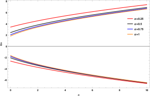
(a) $j=1.\,a=0.1,\,\omega=m=1$

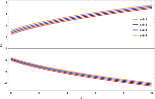
(b) $j=1.\,\alpha=0.5,\,\omega=m=1$

Figure 3: Energy of KGO in rotating cosmic string as a function of the quantum number $n$ for different values of $\alpha$ in (a) and of $a$ in (b).

Hence, after inserting $\vartheta$ and $\delta$ and by solving Eq. ((82)) for $E$, we obtain the energy levels for our scalar particle

$$E^{\pm}(n,\alpha,a,j)=\frac{am\omega}{\alpha}\pm\sqrt{4m\omega n+\left(\frac{am\omega}{\alpha}\right)^{2}+\frac{2m\omega|j|}{\alpha}+m^{2},}$$ (83)

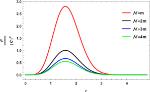
(a) $n=0,\,a=0.1,\,\alpha=0.5$

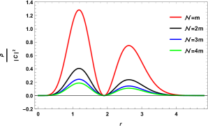
(b) $n=1,\,a=0.1,\,\alpha=0.5$

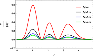
(c) $n=2,\,a=0.1,\,\alpha=0.5$

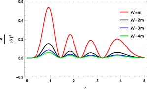
(d) $n=3,\,a=0.1,\,\alpha=0.5$

Figure 4: Plots of the density of KGO in rotating cosmic string as a function of the radial distance $r$ for different values of $n$ with the parameters $a=0.5$ and $j=1.$

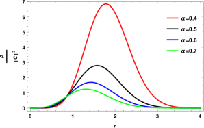
(a) $\mathcal{N}=m,\,a=0.1$

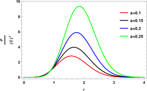
(b) $\mathcal{N}=m,\,\alpha=0.5$

Figure 5: Plots of the density of KGO in rotating cosmic string as a function of the radial distance $r$ for different values of $\alpha$ and $a$ with the parameters $m=\omega=1$ and $j=1.$

As an interesting side result, we have an expression for the energy in which we see all the parameters that characterize the background geometry. Indeed, the energy spectrum does not depend only on the angular deficit parameter $\alpha$, but also on the rotation parameter $a$. We expect that the external gravitational field due to a rotating cosmic string affects on the relativistic dynamics of the quantum particle, essentially, since it has non-zero curvature concentrated along the $z$-axis and its angular momentum appears throughout the parameter $a.$ By comparing the energy ((83)) with the energy of KGO in a static cosmic string ((48)), we notice that $E\left(n,\alpha,a,j\right)$ is shifted by the amount $am\omega\big{/}\alpha$ and enlarged by a conical factor. We plot the energy eigenvalues as a function of the quantum number $n$ with fixed parameters $\omega=j=1$ and for different values of the variable $\alpha$ and $a$ shown in Fig. (3).

Taking this result into the consideration, we can find the density for the FV-KGO in the rotating cosmic string space as a function of the radial distance $r$ and fixed parameter $\alpha$. Fig. (4)shows that the density is affected when choosing the $\mathcal{N}$ variable for different situations. Now, the case where $\mathcal{N}=m$ that corresponds with the case of KGO is presented in the figure. (5). This figure shows that density is strongly dependent with the parameter of rotation $a$.

IV Thermal properties of FVO in Rotating Cosmic String

This section is devoted to look into the thermal properties which may arise throughout our study of the KGO in the space-time produced by a rotating cosmic string. Having already obtained the energy spectrum of KGO in that particular space, we are now in a position to present the thermodynamics of the model encountered in Sec. (III.2) by calculating the partition function which provides all the physical information of our quantum system. To better illustrate our results, we present several figures in the next discussion.

IV.1 Partition function

We are interested in determining the partition function of KGO interacting with the gravitational field induced by rotating cosmic string. Consequently, the statistical quantities such as the free energy $F,$the mean energy $U,$the entropy $S$and the specific heat $C_{v}$, associated with the relativistic spinless particle in that space-time can be obtained from the partition function.

The canonical ensemble partition function at finite temperature $T$ is given by

$$Z=\stackrel{{\scriptstyle[}}{{n}}=0]{\infty}{\sum}e^{-\beta E_{n}},$$ (84)

where $E_{n}$ denotes the corresponding energy eigenvalues and $\beta=\frac{1}{K_{B}T}$ with $K_{B}$ being the Boltzmann constant. Given the spectrum (83) and by considering only the positive energies i.e, $E_{n}=E_{n}^{+}$, we can express the partition function as

$$Z=\stackrel{{\scriptstyle[}}{{n}}=0]{\infty}{\sum}e^{-\beta\left(\mathsf{Y}+\sqrt{\mathsf{A}n+\mathsf{B}}\right)}=e^{-\beta\mathsf{Y}}\stackrel{{\scriptstyle[}}{{n}}=0]{\infty}{\sum}e^{-\beta\sqrt{\mathsf{A}n+\mathsf{B}}},$$ (85)

where

$$\mathsf{Y}=\frac{am\omega}{\alpha},\qquad\mathsf{A}=4m\omega,\qquad\mathsf{B}=\left(\frac{am\omega}{\alpha}\right)^{2}+\frac{2m\omega|j|}{\alpha}+m^{2}$$

In what follows, we closely follow the methods outlined in Ref.(key-88, ) and revised in (key-89, ) with the intention of approximating the infinite sum apparent in Eq. (84). For this purpose, we shall begin with rewriting the series representation of the partition function $Z$ in terms of the Zeta function. Hence we have

$$\stackrel{{\scriptstyle[}}{{n}}=0]{\infty}{\sum}e^{-\beta\sqrt{\mathsf{A}n+\mathsf{B}}}=e^{-\widetilde{\beta}}+\stackrel{{\scriptstyle[}}{{n}}^{\prime}=0]{\infty}{\sum}e^{-\tilde{\beta}\sqrt{\mathsf{D}}\sqrt{\frac{1}{\mathsf{D}}+\left(n^{\prime}+1\right)}},\qquad n=n^{\prime}+1.$$ (86)

where we have introduced the notation

$$\tilde{\beta}=\beta\sqrt{\mathsf{B}},\qquad\mathsf{D=\frac{A}{B}.}$$

Using the Cahen-Mellin integral (key-90, ; key-91, )

$$e^{-\mathit{z}}=\frac{1}{2\pi i}\stackrel{{\scriptstyle[}}{{\mathfrak{}}}{c}-i\infty]{\mathfrak{c}+i\infty}{\int}\Gamma\left(s\right)z^{-s}ds,\qquad\left(|\textrm{arg}z|<\frac{\pi}{2};z\neq 0\right).$$

where the path of integration is the vertical line $\Re(s)=\mathfrak{c}$, with $\mathfrak{c}\in\mathbb{R}^{*}$, lying to the right of all the poles of $\Gamma(s),$ the term $\stackrel{{\scriptstyle[}}{{n}}^{\prime}=0]{\infty}{\sum}e^{-\tilde{\beta}\sqrt{\mathsf{D}}\sqrt{\frac{1}{\mathsf{D}}+\left(n^{\prime}+1\right)}}$ can be expressed as

$$\stackrel{{\scriptstyle[}}{{n}}^{\prime}=0]{\infty}{\sum}e^{-\tilde{\beta}\sqrt{\mathsf{D}}\sqrt{\frac{1}{\mathsf{D}}+\left(n^{\prime}+1\right)}}=\frac{1}{2\pi i}\stackrel{{\scriptstyle[}}{{\mathfrak{}}}{c}-i\infty]{\mathfrak{c}+i\infty}{\int}\left(\tilde{\beta}\sqrt{\mathsf{D}}\right)^{-s}\Gamma\left(s\right)\zeta_{H}\left(\frac{s}{2},\frac{1}{\mathsf{D}}+1\right),$$ (87)

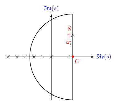
Figure 6: Contour Integration of the Mellin transformation of the problems in question (key-89, ; key-91, )

$\Gamma(s)$ and $\zeta_{H}\left(\frac{s}{2},\frac{1}{\mathsf{D}}+1\right)$ refers to Euler Gamma and Hurwitz zeta functions, receptively. We note that the integral converges only when $s\big{/}2>1$ requires $\mathfrak{c}>2.$ As we need to work out the integral (87), it is clear that the integrand has poles at $s=-k;(k=0,1,2,\cdots)$ of $\Gamma(s),$with residue $(-1)^{k}\big{/}k!$ (see Figure. (6)). In addition, we have a simple pole at $s=2$ of $\zeta_{H}\left(\frac{s}{2},\frac{1}{\mathsf{D}}+1\right)$ with residue equals to $2.$

A straightforward evaluation of the residues at the poles $\{s=0,2,-k\}$ leads to the following expression of the partition function

$$Z(\tilde{\beta})=e^{-\tilde{\beta}\mathsf{YB}^{\nicefrac{{-1}}{{2}}}}\left[-\frac{1}{2}+\frac{1}{\mathsf{D}}\left(\frac{2}{\widetilde{\beta}^{2}}-1\right)+e^{-\widetilde{\beta}}+\stackrel{{\scriptstyle[}}{{n}}=1]{\infty}{\sum}\frac{\left(-\widetilde{\beta}\sqrt{\mathsf{D}}\right)}{n!}^{n}\zeta_{H}\left(-\frac{n}{2},1+\frac{1}{\mathsf{D}}\right)\right],$$ (88)

where we have used the identities

$$\zeta_{H}\left(0,p\right)=\frac{1}{2}-p.$$ (89)

IV.2 Thermal properties

Having estimated the partition function of KGO in rotating cosmic string, we are allowed to compute the main thermodynamic quantities,

$$F=-\frac{\sqrt{B}}{\tilde{\beta}}\ln\left(Z\right),U=-\sqrt{B}\frac{d\ln\left(Z\right)}{d\tilde{\beta}},$$ (90)

$$S=\ln\left(Z\right)-\tilde{\beta}\frac{d\ln\left(Z\right)}{d\tilde{\beta}},\,C_{V}=\tilde{\beta}{}^{2}\frac{d^{2}\ln\left(Z\right)}{d\tilde{\beta}^{2}}.$$

The series representations of the partition function $Z$ in terms of the $\zeta_{H}$-function and the Boltzmann representation introduced in Eq. ((88)) can be evaluated numerically considering only a finite number of terms in the series.

Fig. (7) shows the different thermal quantities of KGO in (2+1)-dimensional rotating cosmic string for $a=0.1$ derived from the partition function keeping $n_{max}=1000$ terms of the series in Eq. ((88)). Following the figure, all thermal quantities are plotted versus a reduced temperature $\tau$: here from the curves of the numerical entropy function, no abrupt change, around $\tau_{0}$ has been identified in the curves of specific heat. This means that the curvature, observed in the specific heat curve does not exhibit or indicate an existence of a phase transition around a $\tau_{0}$ temperature. In addition, the effect of the parameter $\alpha$ for fixed $a$ is well observed in the curves of specific heat. These curves increased when $\alpha$ decreases.

Fig(8) shows the same quantities but for fixed $\alpha=0.5$ and different values of $a.$ As we can see, all the curves of the specific heat coincide a round of $\tau_{0}$ temperature. So, the effect of the rotation on the thermal properties of our oscillator has no effect.

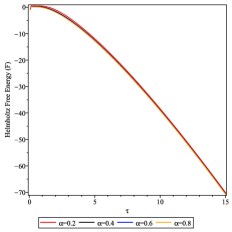
(a) Free energy $F$ versus the reduced temperature $\tau$

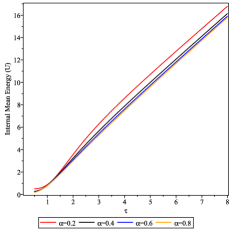
(b) Total energy $U$ versus the reduced temperature $\tau$

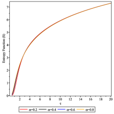
(c) Entropy $S$ versus the reduced temperature $\tau$

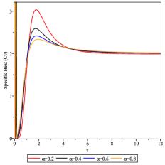
(d) Specific heat $C_{V}$ versus the reduced temperature $\tau$

Figure 7: Statistical functions of KGO in (2+1)-dimensional rotating cosmic string versus $\tilde{\beta}$ for $a=0.1$ and fixed parameters $j=m=\omega=1.$

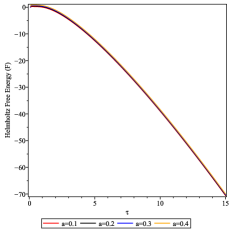
(a) Free energy $F$ versus the reduced temperature $\tau$

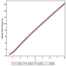
(b) Total energy $U$ versus the reduced temperature $\tau$

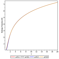
(c) Entropy $S$ versus the reduced temperature $\tau$

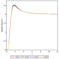
(d) Specific heat $C_{V}$ versus the reduced temperature $\tau$

Figure 8: Statistical functions of KGO in (2+1)-dimensional rotating cosmic string versus $\tilde{\beta}$ for $\alpha=0.5$ and fixed parameters $j=m=\omega=1.$

V Conclusion

The aim of the present work is to study the relativistic dynamics of spinless quantum particle via the Feshbach-Villars representation of two models, namely, the interaction of KGO with the gravitational field generated by the background geometry of : a) static cosmic strings and b) rotating cosmic strings. Starting from the revising the FV formulation of scalar fields in Minkowski space-time, we derived the corresponding formulations in two different curved manifolds. We obtained the exact solutions of both systems and we presented the quantized energy spectra which depend on the parameters that characterize the space-time topology. It is not surprising to find that the wave-function of our quantum system are expressed in terms of the confluent hyper-geometric functions for both static and rotating cosmic strings, since the former can be described throughout the previous one by choosing appropriate coordinate transformation. In our above discussion, we made use of the generalized Feshbach-Villars transformations in order to get relevant observables. Such transformations have been shown to be exact and covers any inertial and gravitational fields. In the last section, we have examined the thermal properties of the system in question by computing the partition function in terms of the Hurwitz zeta function. We have noticed that these thermal quantities are affected by the geometrical and topological parameters of the background geometry.

VI Funding

• Authors report that no funding is available.

VII Author Contribution

• Abdelmalek Buzenada concentrates on programming the system’s thermal properties.

• Abdelmalek Boumali reviews, writes and completes the main text of the manuscript

• All authors reviewed the manuscript

VIII Data Availability Statemen

• The datasets used and/or analysed during the current study available from the corresponding author on reasonable request.

References

- (1) A. Einstein, Annalen Phys. 49, 769 (1916).
- (2) B. P. Abbott et al., Phys Rev Lett 116, 061102 (2016).
- (3) K. Akiyama et al., Astrophys J Lett 875, L1 (2019).
- (4) R. P. Feynman and A. R. Hibbs, Quantum mechanics and path integrals, 1965.
- (5) M. D. Schwartz, Quantum field theory and the standard model, 2013.
- (6) A. Ashtekar and J. J. Stachel, Conceptual problems of quantum gravity, 1991.
- (7) L. Smolin, The trouble with physics : The rise of string theory, the fall of a science, and what comes next, 2006.
- (8) N. D. Birrell and P. Davies, Quantum fields in curved space, 1980.
- (9) L. Parker and D. J. Toms, Quantum field theory in curved spacetime : Quantized fields and gravity, 2009.
- (10) S. W. Hawking, Comm. Math. Phys. 43, 199 (1975).
- (11) W. G. Unruh and R. M. Wald, Phys. Rev. D 25, 942 (1982).
- (12) G. L. Sewell, Ann. Physics 141, 201 (1982).
- (13) T. W. B. Kibble, J. Phys. A 9, 1387 (1976).
- (14) Y. B. Zel’dovich, Mon. Not. R. Astron Soc. 192, 663 (1980).
- (15) A. Vilenkin, Phys. Rep. 121, 263 (1985).
- (16) T. W. B. Kibble, Phys. Rep. 67, 183 (1980).
- (17) A. Vilenkin, Phys. Lett. B 133, 177 (1983).
- (18) A. Vilenkin and E. P. S. Shellard, Cosmic strings and other topological defects, 1985.
- (19) M. Moshinsky and Y. F. Smirnov, The harmonic oscillator in modern physics, 1996.
- (20) A. Ushveridze, Quasi-exactly solvable models in quantum mechanics, 1994.
- (21) D. Itô, K. Mori, and E. W. Carriere, Il Nuovo Cimento A (1965-1970) 51, 1119 (1967).
- (22) M. Moshinsky and A. P. Szczepaniak, J. Phys. A 22 (1989).
- (23) S. A. Bruce and P. C. Minning, Il Nuovo Cimento A (1965-1970) 106, 711 (1993).
- (24) V. V. Dvoeglazov, Il Nuovo Cimento A (1965-1970) 107, 1785 (1994).
- (25) J. Carvalho, A. M. de M. Carvalho, E. Cavalcante, and C. Furtado, Eur. Phys. J. C 76, 1 (2016).
- (26) L. C. dos Santos and C. de Camargo Barros, Eur. Phys. J. C 78, 1 (2017).
- (27) R. L. L. Vitória and K. Bakke, Eur. Phys. J. C 78, 1 (2018).
- (28) R. R. Cuzinatto, M. de Montigny, and P. Pompeia, Class. Quan. Grav 39 (2022).
- (29) F. Ahmed, Europhys. Lett. 131 (2020).
- (30) K. M. Case, Phys Rev 95, 1323 (1954).
- (31) L. L. Foldy, Phys Rev 102, 568 (1956).
- (32) L. L. Foldy and S. A. Wouthuysen, Phys Rev 78, 29 (1950).
- (33) H. Feshbach and F. M. H. Villars, Rev. Modern Phys. 30, 24 (1958).
- (34) B. A. Robson and D. S. Staudte, J. Phys. A : Math. Gen 29, 157 (1996).
- (35) D. S. Staudte, J. Phys. A 29, 169 (1996).
- (36) M. Merad, L. Chetouani, and A. Bounames, Phys. Lett. A 267, 225 (2000).
- (37) A. Bounames and L. Chetouani, Phys. Lett. A 279, 139 (2001).
- (38) S. Haouat and L. Chetouani, Eur. Phys. J. C 41, 297 (2005).
- (39) N. Brown, Z. Papp, and R. M. Woodhouse, Few-Body Systems 57, 103 (2015).
- (40) B. Motamedi, T. Shannon, and Z. Papp, Few-Body Systems (2019).
- (41) O. Klein, Z. Phys 37, 895 (1926).
- (42) W. Gordon, Z. Phys 40, 117 (1926).
- (43) W. Greiner, Relativistic quantum mechanics. wave equations, 2000.
- (44) F. L. Gross, Relativistic quantum mechanics and field theory, 1993.
- (45) A. J. Silenko, Phys. Rev. A 77, 012116 (2008).
- (46) B. Mirza and M. Mohadesi, Commun. Theor. Phys 42, 664 (2004).
- (47) I. Gott, J. R., Astrophys J 288, 422 (1985).
- (48) Hiscock, Phys. Rev. D 31 12, 3288 (1985).
- (49) J. R. Gott and M. Alpert, Gen. Rel. Grav. 16, 243 (1984).
- (50) Gal’tsov and Letelier, Phys. Rev. D 47 10, 4273 (1993).
- (51) A. Boumali and N. Messai, Can. J. Phys. 92, 1460 (2014).
- (52) A. J. Silenko, Theoret. Math. Phys. 156, 1308 (2008).
- (53) A. J. Silenko, Phys. Rev. D 88, 045004 (2013).
- (54) A. Mostafazadeh, J. Phys. A 31, 7829 (1998).
- (55) M. Abramowitz and I. A. Stegun, Handbook of mathematical functions with formulas, graphs, and mathematical tables, volume 55, Dover Publications, New York, 1970.
- (56) E. Bragança, H. S. Mota, and E. B. de Mello, Int J Mod Phys D 24, 1550055 (2015).
- (57) F. Ahmed, Sci Rep 12 (2022).
- (58) G. Arfken, H. Weber, and F. Harris, Mathematical Methods for Physicists : A Comprehensive Guide, Elsevier Science, 2012.
- (59) Mazur, Phys. Rev. Lett 57 8, 929 (1986).
- (60) P. S. Gerbert and R. Jackiw, Comm. Math. Phys. 124, 229 (1989).
- (61) Matsas, Phys. Rev. D 42 8, 2927 (1990).
- (62) Corichi and Pierri, Phys. Rev. D 51 10, 5870 (1995).
- (63) Bekenstein, Phys. Rev. D 45 8, 2794 (1992).
- (64) J. S. Anandan, Phys. Lett. A 195, 284 (1994).
- (65) V. De Lorenci and E. Moreira, Phys. Rev. D 63, 027501 (2000).
- (66) V. De Lorenci and E. Moreira, Nuclear Phys. B Proc. Suppl. 127, 150 (2004).
- (67) M. S. Cunha, C. R. Muniz, H. R. Christiansen, and V. B. Bezerra, Eur. Phys. J. C 76, 1 (2016).
- (68) B.-Q. Wang, Z. W. Long, C.-Y. Long, and S. Wu, Modern Phys. Lett. A 33, 1850025 (2018).
- (69) Z. Wang, Z. W. Long, C.-Y. Long, and B.-Q. Wang, Can. J. Phys. 95, 331 (2017).
- (70) M. Hosseinpour, H. Hassanabadi, and M. de Montigny, Int. J. Geom. Methods Mod. Phys. (2018).
- (71) C. Furtado, F. Moraes, and V. B. Bezerra, Phys. Rev. D 59, 107504 (1999).
- (72) V. De Lorenci and E. Moreira, Phys. Rev. D 70, 047502 (2004).
- (73) V. De Lorenci and E. Moreira, Phys. Lett. B 679, 510 (2009).
- (74) C. Muniz, V. Bezerra, and M. Cunha, Ann. Physics 350, 105 (2014).
- (75) M. Hosseinpour and H. Hassanabadi, Eur. Phys. J. Plus 130, 1 (2015).
- (76) F. Ahmed, Europhys. Lett. 130 (2020).
- (77) F. Ahmed, Modern Phys. Lett. A 35, 2050220 (2020).
- (78) K. Bakke, Eur. Phys. J. Plus 127, 1 (2012).
- (79) K. Bakke, Gen. Rel. Grav. 45, 1847 (2013).
- (80) P. Strange and L. H. Ryder, Phys. Lett. A 380, 3465 (2016).
- (81) B.-Q. Wang, Z.-W. Long, C.-Y. Long, and S.-R. Wu, Int. J. Mod. Phys. A 33, 1850158 (2018).
- (82) M. Hosseinpour, H. Hassanabadi, and M. de Montigny, Eur. Phys. J. C 79, 1 (2019).
- (83) F. Ahmed, Europhys. Lett. 132 (2020).
- (84) M. M. Cunha and E. O. Silva, Adv. High Energy Phys. (2021).
- (85) M. M. Cunha and E. O. Silva, Universe (2020).
- (86) S. Deser, R. Jackiw, and G. ’t Hooft, Ann. Physics 152, 220 (1984).
- (87) Burges, Phys. Rev. D 32 2, 504 (1985).
- (88) A. Boumali, EJTP 12, 121–130 (2015).
- (89) A. M. Frassino, D. Marinelli, O. Panella, and P. Roy, J. Phys. A : Math. Theor. 53 (2020).
- (90) R. B. Paris and D. Kaminski, Asymptotics and mellin-barnes integrals, volume 85, Cambridge University Press, 2001.
- (91) E. Elizalde, Ten physical applications of spectral zeta functions, volume 855, Springer, 2012.