VEM discretization allowing small edges for the reaction-convection-diffusion equation: source and spectral problems

Abstract

In this paper we analyze a lowest order virtual element method for the load classic reaction-convection-diffusion problem and the convection-diffusion spectral problem, where the assumptions on the polygonal meshes allow to consider small edges for the polygons. Under well defined seminorms depending on a suitable stabilization for this geometrical approach, we derive the well posedness of the numerical scheme and error estimates for the load problem, whereas for the spectral problem we derive convergence and error estimates fo the eigenvalues and eigenfunctions. We report numerical tests to asses the performance of the small edges on our numerical method for both problems under consideration.

1 Introduction

Let $\Omega\subset\mathbb{R}^{2}$ be an open, bounded, and convex domain with polygonal boundary $\partial\Omega$. We are interested in the convection-diffusion problem

$$\nabla\cdot(-\kappa(\mathbf{x})\nabla u)+\mathbf{\vartheta}(\mathbf{x})\cdot\nabla u+\gamma(\mathbf{x})u=f\quad\textrm{in}~{}\Omega,\qquad u=0\quad\textrm{on}~{}\partial\Omega,$$ (1.1)

where $\kappa$ and $\gamma$ are smooth functions $\Omega\rightarrow\mathbb{R}$ with $\kappa(\mathbf{x})\geq\kappa_{0}>0$ for all $\mathbf{x}\in\Omega$ and $\mathbf{\vartheta}$ is a smooth vector-valued function $\Omega\rightarrow\mathbb{R}^{2}$.

It is well know that (1.1) is a mathematical model that represents a physical phenomenon involving particles, concentrations, fluids, etc., that are transferred inside a physical system due two processes: convection and diffusion. The eigenvalue problem associated to this system, and variations of it, has been analyzed in the nowadays in [19, 24].

The virtual element method (VEM), introduced in [9] for the first time for the Laplacian operator has shown great accuracy on the approximation of the solutions of partial differential equations, together with important reduction on computational costs, compared with other classic methods. Moreover, since VEM allows different geometries on the meshes, it is possible to implement it with excellent results in problems where partial differential equations are stated in domains which are not suitable, for instance, for the finite element method.

The developments and applications fo VEM are increasing day by day. The literature of VEM is quite extensive, and it is possible to find results in several problems for fluid and solid mechanics, electromagnetism, eigenvalue problems, parabolic problems, and adaptive methods, where primal and mixed formulations have appeared to approximate several problems. We can mention [1, 2, 4, 5, 6, 7, 10, 11, 18, 17, 21, 22, 23, 28, 29, 30] and the references therein.

Despite to the fact of the important contributions of VEM in different subjects, there is a new approach to this method which for the best of the authors knowledge is available for second order elliptic problems, where the standard hypotheses of [9] can be relaxed, and its related to the size of the edges of the elements on the polygonal meshes. We know so far that the classic VEM requires that the elements must be star shaped and with sufficiently large edges. It is precisely this last assumption that is relaxed in the works of [13, 16] where arbitrary edges or feces, depending on the dimension in which the problem is stated, are now allowed. These references show that for more general assumptions, and suitable stabilizations, it is possible to obtain stability of the VEM and error estimates. This is an ongoing subject of research, and the available results are for VEM spaces to discretize $H^{1}$. Also, recently on [3, 20, 27, 32] is possible to find applications of the small edges approach.

It is important to take into account that the theoretical analysis for a VEM allowing small edges needs to pay a price, in the sense that not any system of partial differential equations allows to consider this approach. More precisely, the regularity of the solution plays a role for the analysis. In [13, 16] the authors have shown that when the solution of the PDE is such that $H^{1+s}$ with $s>3/2$, the approximation properties for the VEM with small edges hold. This implies that, under some geometrical hypotheses on the domain, boundary conditions, data, or physical parameters, this new nature of the VEM is possible to be applied. Hence, for our purposes and for the best of our knowledge, we cannot go far from this regularity requirement.

In the present paper, we continue with our research program of VEM with small edges for second order elliptic problems. More precisely, our contribution is to apply this approach on two problems: in one hand, we have the convection-difussion-reaction problem and, on the other, the convection-difussion eigenvalue problem. These two problems are of importance due to the applicability of such equations. For the convection-difussion-reaction problem, we focus on the load problem since in the eigenvalue problem the term associated to the reaction is similar to the right hand side that has the eigenvalue of the problem. This is the reason why we only consider the difussion-convection problem on the spectral setting. Also, since our intention is to apply the small edges scheme for the VEM, as we have claimed before, we need to operate under a suitable geometrical setting which in our case, consists in a open, bounded, and convex two dimensional domain with null Dirichlet boundary conditions. These assumptions will be required for both, the load and spectral problems.

The outline of our manuscript is the following: In section 2 we present the source model problem, the bilinear forms which consider, the well posedness and regularity properties. Section 3 is the core of our paper, where the virtual element methods are introduced, under the assumption of small edges for the polygonal meshes. Here we define the local and global virtual spaces and the discrete bilinear forms. With these ingredients at hand, we discretize the source problem introduced in section 2, proving the well posedeness of the discrete problem and, under the weaker assumptions of the mesh, we derive error estimates. As an application of the derived results so far, in section 5 we analyze the eigenvalue problem associated to (1.1). Since the spectral problem is nonsymmetric, the analysis is performed introducing the adjoint eigenvalue problem. Spurious free, convergence and error estimates results are proved for our proposed VEM. Finally, in section 6 we illustrate the theoretical results of the small edges approach for the source and eigenvalue problem, reporting a set of numerical tests in different contexts and geometries.

2 The variational problem

The weak formulation of (1.1) reads as follows: Find $u\in H_{0}^{1}(\Omega)$ such that

$$\mathcal{B}(u,v)=\mathcal{F}(v)\quad\forall v\in H_{0}^{1}(\Omega),$$ (2.1)

where $\mathcal{B}:H_{0}^{1}(\Omega)\times H_{0}^{1}(\Omega)\rightarrow\mathbb{R}$ is the bilinear form defined by

$$\mathcal{B}(w,v):=a(w,v)+b(w,v)+c(w,v),\quad\forall w,v\in H_{0}^{1}(\Omega),$$ (2.2)

and $\mathcal{F}:H_{0}^{1}(\Omega)\rightarrow\mathbb{R}$ is the functional defined by

$$\mathcal{F}(v)=\int_{\Omega}fv,\quad\forall v\in L^{2}(\Omega),$$ (2.3)

respectively, with $a(\cdot,\cdot)$, $b(\cdot,\cdot)$, and $c(\cdot,\cdot)$ being bounded bilinear forms defined as follows

$$a:H^{1}(\Omega)\times H^{1}(\Omega)\to\mathbb{R};\qquad a(w,v):=\int_{\Omega}\kappa(\mathbf{x})\nabla w\cdot\nabla v,\forall w,v\in H_{0}^{1}(\Omega);\\ b:H^{1}(\Omega)\times L^{2}(\Omega)\to\mathbb{R};\qquad b(w,v):=\int_{\Omega}(\mathbf{\vartheta}(\mathbf{x})\cdot\nabla w)v,\forall w\in H_{0}^{1}(\Omega),v\in L^{2}(\Omega);\\ c:L^{2}(\Omega)\times L^{2}(\Omega)\to\mathbb{R};\qquad c(w,v):=\int_{\Omega}\gamma(\mathbf{x})wv,\forall w,v\in L^{2}(\Omega).$$ (2.4)

The assumptions on the coefficients on (1.1) lead us to the continuity of $\mathcal{B}(\cdot,\cdot)$, i.e, there exists a constant $M_{1}>0$ such that

$$\mathcal{B}(w,v)\leq M_{1}\|w\|_{1,\Omega}\|v\|_{1,\Omega}\quad\forall v,w\in H_{0}^{1}(\Omega).$$ (2.5)

Also, the following condition holds

$$\sup_{v\in H_{0}^{1}(\Omega)}\frac{\mathcal{B}(w,v)}{\|v\|_{1,\Omega}}\geq\beta\|w\|_{1,\Omega}\quad\forall w\in H_{0}^{1}(\Omega),$$ (2.6)

where $\beta>0$ is a constant independent of $v$. Hence, (2.5) and (2.6) implies the well posedness of (2.1).

On the other hand, for the implementation of the virtual element method of our interest, the regularity of (2.1) is a key ingredient in order to obtain approximation properties. Given $f\in H^{-1}$, there exist positive constants $C^{*},C^{**}$ such that the solution $u$ of (2.1) satisfies

$$\|u\|_{1,\Omega}\leq C^{*}\|f\|_{-1,\Omega}\quad\text{and}\quad\|u\|_{2,\Omega}\leq C^{**}\|f\|_{0,\Omega}.$$ (2.7)

3 The virtual element method

In this section we briefly review a virtual element method (VEM) for te system (2.1). First we recall the mesh construction and the assumptions considered in [9] for the virtual element method. Let $\left\{\mathcal{T}_{h}\right\}_{h}$ be a sequence of decompositions of $\Omega$ into polygons, $E$. Let $h_{E}$ denote the diameter of the element $E$ and $h$ the maximum of the diameters of all the elements of the mesh, i.e., $h:=\max_{E\in\Omega}h_{E}$. Moreover, for simplicity in what follows we assume that $\kappa$ and $\gamma$ are piecewise constant with respect to the decomposition $\mathcal{T}_{h}$, i.e., they are piecewise constants for all $E\in\mathcal{T}_{h}$ (see for instance [13]).

For the analysis of the VEM, we will make as in [9] the following assumption: there exists a positive real number $\rho$ such that, for every $E\in\mathcal{T}_{h}$ and for every $\mathcal{T}_{h}$,

• A1. For all meshes $\mathcal{T}_{h}$, each polygon $E\in\mathcal{T}_{h}$ is star-shaped with respect to a ball of radius greater than or equal to $\rho h_{E}$.

For any simple polygon $E$ we define

$$\widetilde{V}_{h}^{E}:=\{v_{h}\in H^{1}(E):\Delta v_{h}\in\mathbb{P}_{1}(E),v_{h}|_{\partial E}\in C^{0}(\partial E),v_{h}|_{e}\in\mathbb{P}_{1}(e)\ \forall e\in\partial E\}.$$

Now, in order to choose the degrees of freedom for $\widetilde{V}_{h}^{E}$ we define

• $\mathcal{V}_{E}^{h}$: the value of $w_{h}$ at each vertex of $E$,

as a set of linear operators from $\widetilde{V}_{h}^{E}$ into $\mathbb{R}$. In [2] it was established that $\mathcal{V}_{E}^{h}$ constitutes a set of degrees of freedom for the space $\widetilde{V}_{h}^{E}$.

On the other hand, we define the projector $\Pi^{\nabla,E}:\ \widetilde{V}_{h}^{E}\longrightarrow\mathbb{P}_{1}(E)\subseteq\widetilde{V}_{h}^{E}$ for each $v_{h}\in\widetilde{V}_{h}^{E}$ as the solution of

$$\int_{E}(\nabla\Pi^{\nabla,E}v_{h}-\nabla v_{h})\cdot\nabla q =0\qquad\forall q\in\mathbb{P}_{1}(E),$$

$$\overline{\Pi^{\nabla,E}v_{h}} =\overline{v_{h}},$$

where for any sufficiently regular function $v$, we set

$$\overline{v}:=|\partial E|^{-1}\int_{\partial E}v.$$

We observe that the term $\Pi^{\nabla,E}v_{h}$ is well defined and computable from the degrees of freedom of $v$ given by $\mathcal{V}_{E}^{h}$, and in addition the projector $\Pi^{\nabla,E}$ satisfies the identity $\Pi^{\nabla,E}(\mathbb{P}_{1}(E))=\mathbb{P}_{1}(E)$ (see for instance [2]).

We are now in position to introduce our local virtual space

$$V^{E}_{h}:=\left\{v_{h}\in\widetilde{V}_{h}^{E}:\displaystyle\int_{E}\Pi^{\nabla,E}v_{h}p=\displaystyle\int_{E}v_{h}p,\quad\forall p\in\mathbb{P}_{1}(E)\right\}.$$ (3.2)

Now, since $V^{E}_{h}\subset\widetilde{V}_{h}^{E}$, the operator $\Pi^{\nabla,E}$ is well defined on $V^{E}_{h}$ and computable only on the basis of the output values of the operators in $\mathcal{V}_{E}^{h}$. In addition, due to the particular property appearing in definition of the space $V^{E}_{h}$, it can be seen that $\forall p\in\mathbb{P}_{1}(E)$ and $\forall v_{h}\in V^{E}_{h}$ the term $(v_{h},p)_{0,E}$ is computable from $\Pi^{\nabla,E}v_{h}$, and hence the ${\mathrm{L}}^{2}(E)$-projector operator $\Pi^{E}:V^{E}_{h}\to\mathbb{P}_{1}(E)$ defined by

$$\int_{E}\Pi^{E}v_{h}=\int_{E}v_{h}p\qquad\forall p\in\mathbb{P}_{1}(E),$$

depends only on the values of the degrees of freedom of $v_{h}$. Actually, it is easy to check that the projectors $\Pi^{\nabla,E}$ and $\Pi^{E}$ are the same operators on the space $V^{E}_{h}$ (see [2] for further details).

Finally, for every decomposition $\mathcal{T}_{h}$ of $\Omega$ into simple polygons $E$ we define the global virtual space

$$V_{h}:=\left\{v\in H^{1}(E):\ v|_{E}\in V^{E}_{h}\quad\forall E\in\mathcal{T}_{h}\right\},$$ (3.3)

and the global degrees of freedom are obtained by collecting the local ones, with the nodal and interface degrees of freedom corresponding to internal entities counted only once those on the boundary are fixed to be equal to zero in accordance with the ambient space $H_{0}^{1}(\Omega)$.

3.1 Discrete formulation

In order to construct the discrete scheme, we need some preliminary definitions. First, we split the bilinear form $\mathcal{B}(\cdot,\cdot)$ as follows:

$$\mathcal{B}(w,v):=\sum_{E\in\mathcal{T}_{h}}\mathcal{B}^{E}(w,v):=\sum_{E\in\mathcal{T}_{h}}a^{E}(w,v)+b^{E}(w,v)+c^{E}(w,v)\,\,\forall w,v\in H^{1}(\Omega),$$

where

$$a^{E}(w,v):=\int_{E}\kappa(x)\nabla w\cdot\nabla v,\quad b^{E}(w,v):=\int_{E}(\mathbf{\vartheta}(x)\cdot\nabla w)v,\quad c^{E}(w,v):=\int_{E}\gamma(x)wv.$$

Now, in order to propose the discrete bilinear form for $a(\cdot,\cdot)$ (cf. (2.4)), we consider the following symmetric and semi-positive definite bilinear form $S^{E}:V^{E}_{h}\times V^{E}_{h}\to\mathbb{R}$ introduced in [13]. For each $E\in\mathcal{T}_{h}$ and for all $w_{h},v_{h}\in V^{E}_{h}$ we set

$$S^{E}(w_{h},v_{h}):=S^{\partial}(w_{h},v_{h}),$$

where, if $\partial_{s}$ denotes a derivative along the edge, $S^{\partial}(\cdot,\cdot)$ is defined by (see [33])

$$S^{\partial}(w_{h},v_{h}):=h_{E}\int_{\partial{E}}\partial_{s}w_{h}\partial_{s}v_{h}\qquad\forall w_{h},v_{h}\in V^{E}_{h}.$$ (3.4)

Then, we introduce on each element $E$ the local (and computable) bilinear forms

• $a_{h}^{E}(w_{h},v_{h}):=a^{E}(\Pi^{\nabla,E}w_{h},\Pi^{\nabla,E}v_{h})+S^{E}(w_{h}-\Pi^{\nabla,E}w_{h},v_{h}-\Pi^{\nabla,E}v_{h})$,

• $b_{h}^{E}(w_{h},v_{h}):=b^{E}(\Pi^{\nabla,E}w_{h},\Pi^{E}v_{h})$,

• $c_{h}^{E}(w_{h},v_{h}):=c^{E}(\Pi^{E}w_{h},\Pi^{E}v_{h})$,

for all $w_{h},v_{h}\in V^{E}_{h}.$

Now we introduce the following discrete semi-norm:

$${\left|\kern-1.07639pt\left|\kern-1.07639pt\left|v\right|\kern-1.07639pt\right|\kern-1.07639pt\right|}_{E}^{2}:=a^{E}\big{(}\Pi^{\nabla,E}v,\Pi^{\nabla,E}v)+S^{E}(v-\bar{v},v-\bar{v})\qquad\forall v\in V^{E}_{h}+\mathcal{V}^{E},$$ (3.5)

where $\mathcal{V}^{E}\subseteq H^{1}(E)$ is a subspace of sufficiently regular functions for $S^{E}(\cdot,\cdot)$ to make sense.

For any sufficiently regular functions, we introduce the following global semi-norms

$${\left|\kern-1.07639pt\left|\kern-1.07639pt\left|v\right|\kern-1.07639pt\right|\kern-1.07639pt\right|}^{2}:=\sum_{E\in\mathcal{T}_{h}}{\left|\kern-1.07639pt\left|\kern-1.07639pt\left|v\right|\kern-1.07639pt\right|\kern-1.07639pt\right|}_{E}^{2},\qquad\left|v\right|_{1,h}^{2}:=\sum_{E\in\mathcal{T}_{h}}\left\|\nabla v\right\|_{0,E}^{2}.$$

It has been proved in [13, Lemma 3.1] the existence of positive constants $C_{1},C_{2},C_{3}$, independent of $h$, but depending on $\kappa$ such that

$$C_{1}{\left|\kern-1.07639pt\left|\kern-1.07639pt\left|v\right|\kern-1.07639pt\right|\kern-1.07639pt\right|}_{E}^{2}\leq a_{h}^{E}(v,v)\leq C_{2}{\left|\kern-1.07639pt\left|\kern-1.07639pt\left|v\right|\kern-1.07639pt\right|\kern-1.07639pt\right|}_{E}^{2}\quad\forall v\in V^{E}_{h},$$ (3.6)

$$a_{h}^{E}(v,v)\leq C_{3}({\left|\kern-1.07639pt\left|\kern-1.07639pt\left|v\right|\kern-1.07639pt\right|\kern-1.07639pt\right|}^{2}+|v|_{1,E}^{2})\quad\forall v\in V^{E}_{h}.$$ (3.7)

In addition, it holds

$$a^{E}(v,v)\leq C_{4}{\left|\kern-1.07639pt\left|\kern-1.07639pt\left|v\right|\kern-1.07639pt\right|\kern-1.07639pt\right|}_{E}^{2}\quad\forall v\in V^{E}_{h},$$ (3.8)

$${\left|\kern-1.07639pt\left|\kern-1.07639pt\left|p\right|\kern-1.07639pt\right|\kern-1.07639pt\right|}_{E}^{2}\leq C_{5}a^{E}(p,p)\quad\forall p\in\mathbb{P}_{1}(E),$$ (3.9)

where $C_{4},C_{5}$ are positive constants independent of $h$.

As is customary, the bilinear form $\mathcal{B}_{h}(\cdot,\cdot)$ can be expressed componentwise as follows

$$\mathcal{B}_{h}(w_{h},v_{h}):=\sum_{E\in\mathcal{T}_{h}}\mathcal{B}_{h}^{E}(w_{h},v_{h})=\sum_{E\in\mathcal{T}_{h}}a_{h}^{E}(w_{h},v_{h})+b_{h}^{E}(w_{h},v_{h})+c_{h}^{E}(w_{h},v_{h}).$$ (3.10)

Now, we are in a position to write the virtual element discretization for problem (2.1): Find $u_{h}\in V_{h}$ such that

$$\mathcal{B}_{h}(u_{h},v_{h})=\mathcal{F}(v_{h})\quad\forall v_{h}\in V_{h},$$ (3.11)

where $\mathcal{F}(v_{h})=\displaystyle(f_{h},v_{h})_{0,\Omega}$ with $f_{h}:=\Pi^{E}f$ and $(\cdot,\cdot)_{0,\Omega}$ denotes the inner product in $L^{2}(\Omega)$. It is clear that $\mathcal{B}_{h}(\cdot,\cdot)$ is continuous, i.e,

$$\mathcal{B}_{h}(w_{h},v_{h})\leq M_{2}{\left|\kern-1.07639pt\left|\kern-1.07639pt\left|w_{h}\right|\kern-1.07639pt\right|\kern-1.07639pt\right|}{\left|\kern-1.07639pt\left|\kern-1.07639pt\left|v_{h}\right|\kern-1.07639pt\right|\kern-1.07639pt\right|}\quad v_{h},w_{h}\in V_{h}^{E},$$ (3.12)

with $M_{2}$ being a constant independent of $h$.

From the definition of the bilinear form $a_{h}(\cdot,\cdot)$, it is easy to check that this discrete bilinear form is coercive in $V_{h}$. Indeed, let $v_{h}\in V_{h}$. Then,

$$a_{h}(v_{h},v_{h})=\sum_{E\in\mathcal{T}_{h}}a_{h}^{E}\big{(}v_{h},v_{h}\big{)}\geq\sum_{E\in\mathcal{T}_{h}}C_{1}{\left|\kern-1.07639pt\left|\kern-1.07639pt\left|v_{h}\right|\kern-1.07639pt\right|\kern-1.07639pt\right|}_{E}^{2}\geq C\sum_{E\in\mathcal{T}_{h}}a^{E}\big{(}v_{h},v_{h}\big{)}\\ \geq C|v_{h}|_{1,\Omega}^{2}\geq\beta\left\|v_{h}\right\|_{1,\Omega}^{2}\qquad\forall v_{h}\in V_{h},$$ (3.13)

where we have used (3.6), (3.8) and the generalized Poincaré inequality.

On the other hand, we also have the following approximation result for polynomials in star-shaped domain (see for instance [15]).

Lemma 1.

If the assumption A1 is satisfied, then there exists a constant $C$, depending only on $k$ and $\gamma$, such that for every $s$ with $0\leq s\leq k$ and for every $v\in H^{1+s}(E)$, there exists $v_{\pi}\in\mathbb{P}_{k}(E)$ such that

$$\left\|v-v_{\pi}\right\|_{0,E}+h_{E}\left|v-v_{\pi}\right|_{1,E}\leq Ch_{E}^{1+s}\left\|v\right\|_{1+s,E}.$$

The next step is to find appropriate terms $u_{I}$ and $u_{\pi}$ that can be used in the above lemma to prove the claimed convergence. For the latter we have the following proposition, which is derived by interpolation between Sobolev spaces (see for instance [25, Theorem I.1.4]) from the analogous result for integer values of $s$. In its turn, the result for integer values is stated in [9, Proposition 4.2] and follows from the classical Scott-Dupont theory (see [15]).

The following, proved in [27, Lemma 4.3], is an extension of [9, Proposition 4.3] to less regular functions.

Lemma 2.

Under the assumption A1, for each $s$ with $0<s\leq k$, there exist $\widehat{\sigma}$ and a constant $C$, depending only on $k$, such that for every $v\in H^{1+s}(\Omega)$, there exists $v_{I}\in V_{h}$ that satisfies

$$\left|v-v_{I}\right|_{1+t,E} \leq Ch_{E}^{s-t}\left|v\right|_{1+s,E}\qquad 0\leq t\leq\min\{\widehat{\sigma},s\},$$

$$\left\|v-v_{I}\right\|_{0,E} \leq Ch_{E}\left|v\right|_{1+s,E}.$$

In order to prove that the virtual element discretization (3.11) is well defined, we need the following technical results.

Lemma 3.

For every $w^{*}\in H_{0}^{1}(\Omega)$ there exists $w^{*}_{h}\in V_{h}$ such that

$$a_{h}(w_{h}^{*},v_{h})=a(w^{*},v_{h})\qquad\forall v_{h}\in V_{h}.$$ (3.14)

Moreover, there exists a constant $C_{\kappa}$, independent of $h$, such that

$$h\|w^{*}-w_{h}^{*}\|_{1,\Omega}+\|w^{*}-w_{h}^{*}\|_{0,\Omega}\leq C_{\kappa}h\|w^{*}\|_{1,\Omega}.$$ (3.15)

Proof.

From (3.13), a simple application of Lax-Milgram lemma implies that (3.14) has a unique solution and ${\left|\kern-1.07639pt\left|\kern-1.07639pt\left|w_{h}^{*}\right|\kern-1.07639pt\right|\kern-1.07639pt\right|}\leq C\|w^{*}\|_{1,\Omega}$. On the other hand, to prove (3.15), we note that:

$$|w^{*}-w_{h}^{*}|_{1,\Omega}^{2} \leq C_{\kappa}(a(w^{*},w^{*}-w_{h}^{*})-a(w_{h}^{*},w^{*}-w_{h}^{*}))$$

$$\leq C_{\kappa}\left(|w^{*}|_{1,\Omega}+|w^{*}_{h}|_{1,\Omega}\right)|w^{*}-w_{h}^{*}|_{1,\Omega}$$

$$\leq\mathcal{C}_{\kappa}\left(|w^{*}|_{1,\Omega}+{\left|\kern-1.07639pt\left|\kern-1.07639pt\left|w_{h}^{*}\right|\kern-1.07639pt\right|\kern-1.07639pt\right|}\right)|w^{*}-w_{h}^{*}|_{1,\Omega}\leq C_{\kappa}|w^{*}|_{1,\Omega}|w^{*}-w_{h}^{*}|_{1,\Omega},$$ (3.16)

where we have used (3.8). Now to control the error in $L^{2}$ norm we use a standard duality argument. Let $\phi\in H^{2}(\Omega)\cap H_{0}^{1}(\Omega)$ be the solution of

$$a(w,\phi)=(w^{*}-w_{h}^{*},w)_{0,\Omega}\qquad w\in H_{0}^{1}(\Omega),$$ (3.17)

and let $\phi_{I}\in V_{h}^{E}$ be its interpolant. Then, from Lemma 2 we have

$$|\phi-\phi_{I}|_{1,\Omega}\leq Ch|\phi|_{2}\leq Ch\|w^{*}-w_{h}^{*}\|_{0,\Omega}.$$ (3.18)

Then, testing (3.17) with $w=w^{*}-w_{h}^{*}\in H_{0}^{1}(\Omega)$, and using (3.14) we obtain

$$\|w^{*}-w_{h}^{*}\|_{0,\Omega}^{2}=a(w^{*}-w_{h}^{*},\phi)=a(w^{*}-w_{h}^{*},\phi-\phi_{I})+a(w^{*}-w_{h}^{*},\phi_{I})\\ =a(w^{*}-w_{h}^{*},\phi-\phi_{I})+a_{h}(w_{h}^{*},\phi_{I})-a(w_{h}^{*},\phi_{I})\\ =a(w^{*}-w_{h}^{*},\phi-\phi_{I})+\sum_{E\in\mathcal{T}_{h}}\left(a_{h}^{E}(w_{h}^{*},\phi_{I}-\Pi^{\nabla,E}\phi_{I})-a^{E}(w_{h}^{*},\phi_{I}-\Pi^{\nabla,E}\phi_{I})\right)\\ \leq C_{\kappa}\left(|w^{*}-w_{h}^{*}|_{1,\Omega}|\phi-\phi_{I}|_{1,\Omega}+\sum_{E\in\mathcal{T}_{h}}{\left|\kern-1.07639pt\left|\kern-1.07639pt\left|w_{h}^{*}\right|\kern-1.07639pt\right|\kern-1.07639pt\right|}_{E}{\left|\kern-1.07639pt\left|\kern-1.07639pt\left|\phi_{I}-\Pi^{\nabla,E}\phi_{I}\right|\kern-1.07639pt\right|\kern-1.07639pt\right|}_{E}\right.\\ \left.+\sum_{E\in\mathcal{T}_{h}}|w_{h}^{*}|_{1,E}|\phi_{I}-\Pi^{\nabla,E}\phi_{I}|_{1,E}\right)\\ \leq C_{\kappa}\left(h\|w^{*}\|_{1,\Omega}|\phi|_{2,\Omega}+\sum_{E\in\mathcal{T}_{h}}{\left|\kern-1.07639pt\left|\kern-1.07639pt\left|w_{h}^{*}\right|\kern-1.07639pt\right|\kern-1.07639pt\right|}_{E}{\left|\kern-1.07639pt\left|\kern-1.07639pt\left|\phi_{I}-\Pi^{\nabla,E}\phi_{I}\right|\kern-1.07639pt\right|\kern-1.07639pt\right|}_{E}\right),$$ (3.19)

where, for the last estimate, we have used (3.1), (3.18) and (3.8). The following step is to bound the last term of the above estimate. With this purpose, we first note that from (3.6), the definition of $a_{h}^{E}(\cdot,\cdot)$ and operating as in the proof of [13, Theorem 4.5], together with the fact that $\Pi^{\nabla,E}\phi_{I}$ is the best approximation of $\phi_{I}$ through polynomials of degree $k$, we obtain

$$C_{1} {\left|\kern-1.07639pt\left|\kern-1.07639pt\left|\phi_{I}-\Pi^{\nabla,E}\phi_{I}\right|\kern-1.07639pt\right|\kern-1.07639pt\right|}_{E}^{2}\leq a_{h}^{E}(\phi_{I}-\Pi^{\nabla,E}\phi_{I},\phi_{I}-\Pi^{\nabla,E}\phi_{I})$$

$$=S^{E}(\phi_{I}-\Pi^{\nabla,E}\phi_{I},\phi_{I}-\Pi^{\nabla,E}\phi_{I})\leq h_{E}|\phi_{I}-\Pi^{\nabla,E}\phi_{I}|_{1,\partial E}^{2}$$

$$\leq C_{\kappa}(|\phi_{I}-\Pi^{\nabla,E}\phi_{I}|_{1,E}^{2}+h^{2}|\phi_{I}|_{2,E}^{2}.)$$

$$\leq C_{\kappa}(|\phi_{I}-\Pi^{\nabla,E}\phi|_{1,E}^{2}+h^{2}|\phi_{I}-\phi|_{2,E}^{2}+h^{2}|\phi|_{2,E}^{2})\leq Ch^{2}|\phi|_{2,E}^{2},$$

allowing us to conclude that

$$\sum_{E\in\mathcal{T}_{h}}{\left|\kern-1.07639pt\left|\kern-1.07639pt\left|w_{h}^{*}\right|\kern-1.07639pt\right|\kern-1.07639pt\right|}_{E}{\left|\kern-1.07639pt\left|\kern-1.07639pt\left|\phi_{I}-\Pi^{\nabla,E}\phi_{I}\right|\kern-1.07639pt\right|\kern-1.07639pt\right|}_{E}\leq Ch{\left|\kern-1.07639pt\left|\kern-1.07639pt\left|w_{h}^{*}\right|\kern-1.07639pt\right|\kern-1.07639pt\right|}|\phi|_{2,\Omega}.$$

Therefore, from the above estimation, together with (3.8), (3.19) and the fact that ${\left|\kern-1.07639pt\left|\kern-1.07639pt\left|w_{h}^{*}\right|\kern-1.07639pt\right|\kern-1.07639pt\right|}\leq C\|w^{*}\|_{1,\Omega}$, we obtain

$$\|w^{*}-w_{h}^{*}\|_{0,\Omega}^{2}\leq C_{\kappa}h\|w^{*}\|_{1,\Omega}\|w^{*}-w_{h}^{*}\|_{0,\Omega}.$$

This concludes the proof. ∎

In order to state the well posedness of the discrete problem (3.11), the following discrete inf-sup condition is essential.

Lemma 4.

There exists a constant $\widehat{\beta}>0$ such that, for all $h<h_{0}$:

$$\sup_{w_{h}\in V_{h}}\frac{\mathcal{B}_{h}(v_{h},w_{h})}{\|w_{h}\|_{1,\Omega}}\geq\widehat{\beta}\|v_{h}\|_{1,\Omega}\quad\forall v_{h}\in V_{h}.$$ (3.20)

Proof.

To prove this result we resort to the classic construction of the Fortin operator. From the continuous inf-sup condition (2.6), for $v_{h}\in V_{h}$, there exists $w^{*}\in H_{0}^{1}(\Omega)$ such that

$$\frac{\mathcal{B}(v_{h},w^{*})}{\|w^{*}\|_{1,\Omega}}\geq M_{2}\|v_{h}\|_{1,\Omega}.$$ (3.21)

From Lemma 3 the following problem

$$\text{Find }w_{h}^{*}\in V_{h}\text{ such that }a_{h}(w_{h}^{*},v_{h})=a(w^{*},v_{h}),$$

has a unique solution which satisfies

$${\left|\kern-1.07639pt\left|\kern-1.07639pt\left|w_{h}^{*}\right|\kern-1.07639pt\right|\kern-1.07639pt\right|}\leq\|w^{*}\|_{1,\Omega},\qquad\|w_{h}^{*}-w^{*}\|_{0,\Omega}\leq h\|w^{*}\|_{1,\Omega}.$$ (3.22)

On the other hand, elementary algebraic manipulations, together with the use of the properties of the virtual projector, lead to

$$\mathcal{B}_{h}(v_{h},w_{h}^{*}) =a_{h}(v_{h},w_{h}^{*})+b_{h}(v_{h},w_{h}^{*})+c_{h}(v_{h},w_{h}^{*})$$

$$=a(v_{h},w^{*})+b_{h}(v_{h},w_{h}^{*})-b(v_{h},w^{*})+c_{h}(v_{h},w_{h}^{*})-c(v_{h},w^{*})$$

$$+b(v_{h},w^{*})+c(v_{h},w^{*})$$

$$=\mathcal{B}(v_{h},w^{*})+b_{h}(v_{h},w_{h}^{*})-b(v_{h},w^{*})+c_{h}(v_{h},w_{h}^{*})-c(v_{h},w^{*})$$

$$=\mathcal{B}(v_{h},w^{*})+b_{h}(v_{h},w_{h}^{*})-b(v_{h},w_{h}^{*})+c_{h}(v_{h},w_{h}^{*})-c(v_{h},w_{h}^{*})$$

$$+b(v_{h},w_{h}^{*}-w^{*})+c(v_{h},w_{h}^{*}-w^{*}).$$

Reorganizing the computations above, in order to simplify the presentation of the matetrial, we have

$$\mathcal{B}_{h}(v_{h},w_{h}^{*})+\underbrace{b(v_{h},w^{*}-w_{h}^{*})}_{T_{1}} +\underbrace{c(v_{h},w^{*}-w_{h}^{*})}_{T_{2}}$$

$$+\underbrace{c(v_{h},w_{h}^{*})-c_{h}(v_{h},w_{h}^{*})}_{T_{3}} +\underbrace{b(v_{h},w_{h}^{*})-b_{h}(v_{h},w_{h}^{*})}_{T_{4}}=\mathcal{B}(v_{h},w^{*}).$$ (3.23)

Now our task is to estimate each of the terms $T_{i}$, $i\in\{1,2,3,4\}$, independently of the meshsize $h$. We begin with $T_{1}$. Observe that using that fact that $b(\cdot,\cdot)$ is bounded, together with (3.22), we obtain

$$T_{1}\leq C_{\mathbf{\vartheta}}h\|v_{h}\|_{1,\Omega}\|w^{*}\|_{1,\Omega}.$$ (3.24)

For the term $T_{2}$, a simple application of the Cauchy-Schwarz inequality, together with (3.22), leads to

$$T_{2}\leq C_{\gamma}h\|v_{h}\|_{1,\Omega}\|w^{*}\|_{1,\Omega}.$$

For $T_{3}$, using that $\gamma(\mathbf{x})$ is piecewise constant with respect to the meshes, together with the properties of projector $\Pi^{E}$ and (3.22), we have

$$T_{3}=\sum_{E\in\mathcal{T}_{h}}c^{E}(v_{h},w_{h}^{*})-c_{h}^{E}(v_{h},w_{h}^{*})=\sum_{E\in\mathcal{T}_{h}}c^{E}(v_{h},w_{h}^{*}-\Pi^{E}w_{h}^{*})-c_{h}^{E}(v_{h},w_{h}^{*}-\Pi^{E}w_{h}^{*})\\ \leq\sum_{E\in\mathcal{T}_{h}}c_{\gamma}\|v_{h}\|_{0,E}\|w_{h}^{*}-\Pi^{E}w_{h}^{*}\|_{0,E}\leq\sum_{E\in\mathcal{T}_{h}}c_{\gamma}h_{E}\|v_{h}\|_{0,E}|w_{h}^{*}|_{1,E}\\ \leq\sum_{E\in\mathcal{T}_{h}}c_{\gamma,\kappa}h_{E}C_{4}\|v_{h}\|_{0,E}{\left|\kern-1.07639pt\left|\kern-1.07639pt\left|w_{h}^{*}\right|\kern-1.07639pt\right|\kern-1.07639pt\right|}_{E}\leq C_{\gamma,\kappa}h\|v_{h}\|_{1,\Omega}{\left|\kern-1.07639pt\left|\kern-1.07639pt\left|w_{h}^{*}\right|\kern-1.07639pt\right|\kern-1.07639pt\right|}\leq C_{\gamma,\kappa}h\|v_{h}\|_{1,\Omega}\|w^{*}\|_{1,\Omega},$$

where we have used that $\kappa(\mathbf{x})$ is piecewise constant with respect to the meshes, together with (3.8) and (3.22). For the term $T_{4}$, first, it is necessary to note the following relation

$$b^{E}(v_{h},w_{h}^{*}) -b_{h}^{E}(v_{h},w_{h}^{*})=\left(\mathbf{\vartheta}(\mathbf{x})\cdot\nabla v_{h},w_{h}^{*}\right)_{0,E}-\left(\mathbf{\vartheta}(\mathbf{x})\cdot\nabla\Pi^{\nabla,E}v_{h},\Pi^{E}w_{h}^{*}\right)_{0,E}$$

$$=\left(\mathbf{\vartheta}(\mathbf{x})\cdot\nabla v_{h},w_{h}^{*}-\Pi^{E}w_{h}^{*}\right)_{0,E}+\left(\mathbf{\vartheta}(\mathbf{x})\cdot(\nabla v_{h}-\nabla\Pi^{\nabla,E}v_{h}),\Pi^{E}w_{h}^{*}\right)_{0,E}$$

$$=\left(\mathbf{\vartheta}(\mathbf{x})\cdot\nabla v_{h}-\Pi^{E}(\mathbf{\vartheta}(\mathbf{x})\cdot\nabla v_{h}),w_{h}^{*}-\Pi^{E}w_{h}^{*}\right)_{0,E}$$

$$+\left(\nabla v_{h}-\nabla\Pi^{\nabla,E}v_{h},\mathbf{\vartheta}(\mathbf{x})\Pi^{E}w_{h}^{*}-\mathbf{\vartheta}(\mathbf{x})w_{h}^{*}\right)_{0,E}$$

$$+\left(\nabla v_{h}-\nabla\Pi^{\nabla,E}v_{h},\mathbf{\vartheta}(\mathbf{x})w_{h}^{*}-\Pi^{E}(\mathbf{\vartheta}(\mathbf{x})w_{h}^{*})\right)_{0,E},$$

where we have used the properties of the virtual projector. Therefore, we have the following estimate

$$b^{E}(v_{h},w_{h}^{*})-b_{h}^{E}(v_{h},w_{h}^{*})\leq\|\mathbf{\vartheta}(\mathbf{x})\cdot\nabla v_{h}-\Pi_{1}^{E}(\mathbf{\vartheta}(\mathbf{x})\cdot\nabla v_{h})\|_{0,E}\|w_{h}^{*}-\Pi^{E}w_{h}^{*}\|_{0,E}\\ +\|\nabla v_{h}-\nabla\Pi^{\nabla,E}v_{h}\|_{0,E}\|\mathbf{\vartheta}(\mathbf{x})\Pi^{E}w_{h}^{*}-\mathbf{\vartheta}(\mathbf{x})w_{h}^{*}\|_{0,E}\\ +\|\nabla v_{h}-\nabla\Pi^{\nabla,E}v_{h}\|_{0,E}\|\mathbf{\vartheta}(\mathbf{x})w_{h}^{*}-\Pi^{E}(\mathbf{\vartheta}(\mathbf{x})w_{h}^{*})\|_{0,E}\\ \leq h_{E}C_{\mathbf{\vartheta}}\|v_{h}\|_{1,E}|w_{h}^{*}|_{1,E}\leq h_{E}C_{\mathbf{\vartheta}}\|v_{h}\|_{1,E}{\left|\kern-1.07639pt\left|\kern-1.07639pt\left|w_{h}^{*}\right|\kern-1.07639pt\right|\kern-1.07639pt\right|}_{E}.$$

Thus, summing over all the elements we have that

$$T_{4}\leq hC_{\mathbf{\vartheta}}\|v_{h}\|_{1,\Omega}{\left|\kern-1.07639pt\left|\kern-1.07639pt\left|w_{h}^{*}\right|\kern-1.07639pt\right|\kern-1.07639pt\right|}\leq C_{\kappa,\mathbf{\vartheta}}h\|v_{h}\|_{1,\Omega}\|w^{*}\|_{1,\Omega}.$$

Therefore, from (3.24), together with (3.21) and (3.23) we get that

$$C_{\gamma,\kappa,\mathbf{\vartheta}}h\|v_{h}\|_{1,\Omega}\|w^{*}\|_{1,\Omega}+\mathcal{B}_{h}(v_{h},w_{h}^{*})\geq\mathcal{B}(v_{h},w^{*})\geq M_{2}\|v_{h}\|_{1,\Omega}\|w^{*}\|_{1,\Omega}.$$

Then we have

$$\mathcal{B}_{h}(v_{h},w_{h}^{*})\geq(M_{2}-C_{\gamma,\kappa,\mathbf{\vartheta}}h)\|v_{h}\|_{1,\Omega}\|w^{*}\|_{1,\Omega}.$$ (3.25)

On the other hand, using (3.22), (3.8), together to (3.13), we obtain

$$\|w^{*}\|_{1,\Omega}^{2}\geq{\left|\kern-1.07639pt\left|\kern-1.07639pt\left|w_{h}^{*}\right|\kern-1.07639pt\right|\kern-1.07639pt\right|}^{2}=\sum_{E\in\mathcal{T}_{h}}{\left|\kern-1.07639pt\left|\kern-1.07639pt\left|w_{h}^{*}\right|\kern-1.07639pt\right|\kern-1.07639pt\right|}_{E}^{2}\geq\sum_{E\in\mathcal{T}_{h}}\dfrac{1}{C_{4}}a^{E}(w_{h}^{*},w_{h}^{*})\geq\beta\|w_{h}^{*}\|_{1,\Omega}^{2}.$$ (3.26)

Hence, using (3.25) and (3.26) it is straightforward to check that there exists $h_{0}>0$ such that for all $h<h_{0}$, the inf-sup condition (3.20) holds true. ∎

With these results at hand, we are in position to conclude the following result that establishes the well posedness of (3.11)

Theorem 5 (Well posedeness).

For a given $f\in L^{2}(\Omega)$ and for $h$ sufficiently small, there exists a unique $u_{h}\in V_{h}$ solution of problem (3.11). Moreover, there exists a positive constant $C>0$, independent of $h$, such that $\|u_{h}\|_{1,\Omega}\leq C\|f\|_{0,\Omega}$.

4 A priori error estimates

In this section we derive a priori error estimates for our virtual element method. To do this task, first we remark that we are considering (3.4) as stabilization of the method under the small edges approach. This motivates to adapt the results of [13, Section 4.2] for our problem, where the error estimates (more precisely the constants on each estimate) depend on the geometrical assumptions.

Now our goal is to derive error estimates for our proposed virtual element method. We prove two error estimates: in one hand, we prove an $H^{1}$ error for the solution, and in the other an $L^{2}$ estimate. We begin with the $H^{1}$ estimate.

Theorem 6.

Let $u\in H^{2}(\Omega)\cap H^{1}(\Omega)$ and $u_{h}\in V_{h}$ be the unique solutions of the continuous and discrete problems (2.1) and (3.11), respectively. Then, for $h$ sufficiently small, there exists $C_{\gamma,\kappa,\mathbf{\vartheta}}>0$, independent of h, such that

$$\|u-u_{h}\|_{1,\Omega}\leq C_{\gamma,\kappa,\mathbf{\vartheta}}h\|f\|_{1,\Omega}.$$

Proof.

From triangle inequality we have

$$\|u-u_{h}\|_{1,\Omega}\leq\|u-u_{I}\|_{1,\Omega}+\|u_{h}-u_{I}\|_{1,\Omega}.$$ (4.1)

where we need to estimate each of the terms on the right hand side. We observe that the first term is directly controlled thanks to Lemma 2. The main task is to bound the second term. With this in mind, we set $v_{h}:=u_{h}-u_{I}$ in (3.20). Then

$$\widehat{\beta}\|u_{h}-u_{I}\|_{1,\Omega}\|w_{h}^{*}\|_{1,\Omega} \leq\mathcal{B}_{h}(u_{h},w_{h}^{*})-\mathcal{B}_{h}(u_{I},w_{h}^{*})$$

$$=(f_{h}-f,w_{h}^{*})_{0,\Omega}+\mathcal{B}_{h}(\Pi^{\nabla}u-u_{I},w_{h}^{*})+\mathcal{B}(u-\Pi^{\nabla}u,w_{h}^{*})$$

$$+\mathcal{B}(\Pi^{\nabla}u,w_{h}^{*})-\mathcal{B}_{h}(\Pi^{\nabla}u,w_{h}^{*}),$$ (4.2)

where we have used, (2.1), (3.11), and elementary algebraic manipulations. Then, for the Cauchy–Schwarz inequality, we have

$$\left(f_{h}-f,w_{h}^{*}\right)_{0,\Omega}\leq\|f_{h}-f\|_{0,\Omega}\|w_{h}^{*}\|_{0,\Omega}\leq Ch\|f\|_{1,\Omega}\|w_{h}^{*}\|_{1,\Omega}.$$ (4.3)

On the other hand, from (2.5) and (3.12), we obtain

$$\mathcal{B}_{h}(\Pi^{\nabla}u-u_{I},w_{h}^{*})+\mathcal{B}(u-\Pi^{\nabla}u,w_{h}^{*})\\ \leq C_{\gamma,\kappa,\mathbf{\vartheta}}\left({\left|\kern-1.07639pt\left|\kern-1.07639pt\left|\Pi^{\nabla}u-u_{I}\right|\kern-1.07639pt\right|\kern-1.07639pt\right|}{\left|\kern-1.07639pt\left|\kern-1.07639pt\left|w_{h}^{*}\right|\kern-1.07639pt\right|\kern-1.07639pt\right|}+\|u-\Pi^{\nabla}u\|_{1,\Omega}\|w_{h}^{*}\|_{1,\Omega}\right)\\ \leq C_{\gamma,\kappa,\mathbf{\vartheta}}\big{(}\left({\left|\kern-1.07639pt\left|\kern-1.07639pt\left|\Pi^{\nabla}u-u\right|\kern-1.07639pt\right|\kern-1.07639pt\right|}+{\left|\kern-1.07639pt\left|\kern-1.07639pt\left|u-u_{I}\right|\kern-1.07639pt\right|\kern-1.07639pt\right|}\right){\left|\kern-1.07639pt\left|\kern-1.07639pt\left|w_{h}^{*}\right|\kern-1.07639pt\right|\kern-1.07639pt\right|}+\|u-\Pi^{\nabla}u\|_{1,\Omega}{\left|\kern-1.07639pt\left|\kern-1.07639pt\left|w_{h}^{*}\right|\kern-1.07639pt\right|\kern-1.07639pt\right|}\big{)}.$$

The following step is to bound each of the terms on the right-hand side of the previous estimate. To do this task, using the definition of ${\left|\kern-1.07639pt\left|\kern-1.07639pt\left|\cdot\right|\kern-1.07639pt\right|\kern-1.07639pt\right|}$ (cf. (3.5)) and, again operating as in the proof of [13, Theorem 4.5], we get

$${\left|\kern-1.07639pt\left|\kern-1.07639pt\left|u-u_{I}\right|\kern-1.07639pt\right|\kern-1.07639pt\right|}^{2}=\sum_{E\in\mathcal{T}_{h}}{\left|\kern-1.07639pt\left|\kern-1.07639pt\left|u-u_{I}\right|\kern-1.07639pt\right|\kern-1.07639pt\right|}_{E}=\sum_{E\in\mathcal{T}_{h}}\left\{a^{E}(\Pi^{\nabla,E}(u-u_{I}),\Pi^{\nabla,E}(u-u_{I}))\right.$$

$$\left.+S^{E}(u-u_{I}-\overline{(u-u_{I})},u-u_{I}-\overline{(u-u_{I})})\right\}$$

$$\leq C_{\kappa}\sum_{E\in\mathcal{T}_{h}}\left\{|\Pi^{\nabla,E}(u-u_{I})|_{1,E}^{2}+S^{E}(u-u_{I},u-u_{I})\right\}$$

$$\leq C_{\kappa}\sum_{E\in\mathcal{T}_{h}}\left\{|u-u_{I}|_{1,E}^{2}+h_{E}|u-u_{I}|_{1,\partial E}^{2}\right\}\leq C_{\kappa}\sum_{E\in\mathcal{T}_{h}}h_{E}^{2}|u|_{2,E}^{2}\leq C_{\kappa}h^{2}|u|_{2,\Omega}^{2},$$

where we have used a scaled trace inequality (see [13, Lemma 6.1]). Similarly, using also standard approximation results on polygons, we obtain

$${\left|\kern-1.07639pt\left|\kern-1.07639pt\left|\Pi^{\nabla}u-u\right|\kern-1.07639pt\right|\kern-1.07639pt\right|}\leq C_{\kappa}h|u|_{2,\Omega}.$$

On the other hand, invoking Lemma 1, we have $\|u-\Pi^{\nabla}u\|_{1,\Omega}\leq C\|u\|_{2,\Omega}$. Thus, from the above estimates we conclude that

$$\mathcal{B}_{h}(\Pi^{\nabla}u-u_{I},w_{h}^{*})+\mathcal{B}(u-\Pi^{\nabla}u,w_{h}^{*})\leq C_{\gamma,\kappa,\mathbf{\vartheta}}h\|u\|_{2,\Omega}{\left|\kern-1.07639pt\left|\kern-1.07639pt\left|w_{h}^{*}\right|\kern-1.07639pt\right|\kern-1.07639pt\right|}.$$

We now need a control for the term ${\left|\kern-1.07639pt\left|\kern-1.07639pt\left|w_{h}^{*}\right|\kern-1.07639pt\right|\kern-1.07639pt\right|}$. To do this task, we invoke Lemma 3 with $\|w^{*}\|_{1,\Omega}=1$. Moreover, there exists a constant $\widetilde{C}>0$ such that:

$${\left|\kern-1.07639pt\left|\kern-1.07639pt\left|w_{h}^{*}\right|\kern-1.07639pt\right|\kern-1.07639pt\right|}^{2}\leq\sum_{E\in\mathcal{T}_{h}}a_{h}^{E}(w_{h}^{*},w_{h}^{*})=a_{h}(w_{h}^{*},w_{h}^{*})=a(w^{*},w_{h}^{*})\leq C_{\kappa}\|w^{*}\|_{1,\Omega}\|w_{h}^{*}\|_{1,\Omega}\\ \ \leq C_{\kappa}(1+\|w_{h}^{*}\|_{1,\Omega}^{2})\leq(\widetilde{C}+1)\|w_{h}^{*}\|_{1,\Omega}^{2}.$$

Then we have

$$\mathcal{B}_{h}(\Pi^{\nabla}u-u_{I},w_{h}^{*})+\mathcal{B}(u-\Pi^{\nabla}u,w_{h}^{*})\leq C_{\gamma,\kappa,\mathbf{\vartheta}}h\|u\|_{2,\Omega}\|w_{h}^{*}\|_{1,\Omega}.$$ (4.4)

Finally, we need to control the last term of (4.2). With this purpose, using that $\kappa(\mathbf{x})$ and $\gamma(\mathbf{x})$ are piecewise constant with respect to the meshes, together with the definitions of the bilinear forms $a_{h}^{E}(\cdot,\cdot)$, $b_{h}^{E}(\cdot,\cdot)$, $c_{h}^{E}(\cdot,\cdot)$, the properties of the virtual projectors and Lemma 1, we have

$$\mathcal{B}(\Pi^{\nabla}u,w_{h}^{*})-\mathcal{B}_{h}(\Pi^{\nabla}u,w_{h}^{*})=b(\Pi^{\nabla}u,w_{h}^{*}-\Pi^{\nabla}w_{h}^{*})\\ \leq C_{\mathbf{\vartheta}}|\Pi^{\nabla,E}u|_{1,\Omega}\|w_{h}^{*}-\Pi^{\nabla}w_{h}^{*}\|_{0,\Omega}\\ \leq C_{\mathbf{\vartheta}}|u|_{1,\Omega}\|w_{h}^{*}-\Pi w_{h}^{*}\|_{0,\Omega}\leq hC_{\mathbf{\vartheta}}\|u\|_{1,\Omega}\|w_{h}^{*}\|_{1,\Omega}.$$ (4.5)

Then, gathering (4.3), (4.4), (4.5) and replacing these estimates in (4.2), together with the approximation property given by Lemma 2 in (4.1), we conclude the proof. ∎

Theorem 7.

Let $u\in H^{2}(\Omega)\cap H^{1}(\Omega)$ and $u_{h}\in V_{h}$ be the unique solutions of the continuous and discrete formulations (2.1) and (3.11), respectively. Then, for $h$ sufficiently small, there exists $C_{\gamma,\kappa,\mathbf{\vartheta}}>0$, independent of h, such that

$${\left|\kern-1.07639pt\left|\kern-1.07639pt\left|u-u_{h}\right|\kern-1.07639pt\right|\kern-1.07639pt\right|}\leq C_{\gamma,\kappa,\mathbf{\vartheta}}h\|f\|_{1,\Omega}.$$

Proof.

From triangle inequality we have ${\left|\kern-1.07639pt\left|\kern-1.07639pt\left|u-u_{h}\right|\kern-1.07639pt\right|\kern-1.07639pt\right|}\leq{\left|\kern-1.07639pt\left|\kern-1.07639pt\left|u-u_{I}\right|\kern-1.07639pt\right|\kern-1.07639pt\right|}+{\left|\kern-1.07639pt\left|\kern-1.07639pt\left|u_{h}-u_{I}\right|\kern-1.07639pt\right|\kern-1.07639pt\right|}$. Let $v_{h}:=u_{h}-u_{I}\in V_{h}$. From (3.6), we obtain

$${\left|\kern-1.07639pt\left|\kern-1.07639pt\left|u_{h}-u_{I}\right|\kern-1.07639pt\right|\kern-1.07639pt\right|}^{2}=\sum_{E\in\mathcal{T}_{h}}{\left|\kern-1.07639pt\left|\kern-1.07639pt\left|u_{h}-u_{I}\right|\kern-1.07639pt\right|\kern-1.07639pt\right|}_{E}^{2}\\ \leq\sum_{E\in\mathcal{T}_{h}}\dfrac{1}{c_{1}}a_{h}^{E}(u_{h}-u_{I},v_{h})\leq C\left(\sum_{E\in\mathcal{T}_{h}}\left(a_{h}^{E}(u_{h}-,v_{h})-a_{h}^{E}(u_{I},v_{h})\right)\right)\\ \leq C\left((f_{h},v_{h})-\sum_{E\in\mathcal{T}_{h}}\left(b_{h}^{E}(u_{h},v_{h})+c_{h}^{E}(u_{h},v_{h})\right)\right.\\ \left.-\sum_{E\in\mathcal{T}_{h}}\left[a_{h}^{E}(u_{I}-u_{\pi},v_{h})+a^{E}(u_{\pi}-u,v_{h})+a^{E}(u,v_{h})\right]\right)\\ \leq C\left((f_{h},v_{h})-(f,v_{h})+\sum_{E\in\mathcal{T}_{h}}\left(b^{E}(u,v_{h})-b_{h}^{E}(u_{h},v_{h})+c^{E}(u,v_{h})-c_{h}^{E}(u_{h},v_{h})\right)\right.\\ \left.-\sum_{E\in\mathcal{T}_{h}}\left[a_{h}^{E}(u_{I}-u_{\pi},v_{h})+a^{E}(u_{\pi}-u,v_{h})\right]\right).$$

Now we need to estimate each term on the right-hand side of the above estimate. With this goal in mind, we proceed as in the proof of Lemma 4 and Theorem 6, so we obtain the following estimates

$$(f_{h},v_{h})_{0,\Omega}-(f,v_{h})_{0,\Omega} \leq Ch\|f\|_{1,\Omega}\|v_{h}\|_{1,\Omega},$$

$$\sum_{E\in\mathcal{T}_{h}}(b^{E}(u,v_{h})-b_{h}^{E}(u_{h},v_{h})) \leq C_{\kappa,\mathbf{\vartheta}}h\|u\|_{2,\Omega}\|v_{h}\|_{1,\Omega},$$

$$\sum_{E\in\mathcal{T}_{h}}(c^{E}(u,v_{h})-c_{h}^{E}(u_{h},v_{h})) \leq C_{\gamma,\kappa}h\|u\|_{1,\Omega}\|w_{h}\|_{1,\Omega},$$

$$\sum_{E\in\mathcal{T}_{h}}(a_{h}^{E}(u_{I}-u_{\pi},v_{h})+a^{E}(u_{\pi}-u,v_{h})) \leq C_{\kappa}h\|u\|_{2,\Omega}{\left|\kern-1.07639pt\left|\kern-1.07639pt\left|v_{h}\right|\kern-1.07639pt\right|\kern-1.07639pt\right|}.$$

Combining all these estimates we obtain

$${\left|\kern-1.07639pt\left|\kern-1.07639pt\left|u_{h}-u_{I}\right|\kern-1.07639pt\right|\kern-1.07639pt\right|}^{2}\leq C_{\gamma,\kappa,\mathbf{\vartheta}}h(\|f\|_{1,\Omega}+\|u\|_{2,\Omega}){\left|\kern-1.07639pt\left|\kern-1.07639pt\left|u_{h}-u_{I}\right|\kern-1.07639pt\right|\kern-1.07639pt\right|},$$

which concludes the proof. ∎

Our next goal is to improve the error estimate for the $L^{2}$-norm. This is contained in the following result.

Theorem 8.

For $h$ sufficiently small, the following error estimate holds:

$$\|u-u_{h}\|_{0,\Omega}\leq C_{\kappa,\mathbf{\vartheta},\gamma}h^{2}\|f\|_{0,\Omega}.$$

Proof.

We procede with a standard duality argument. Let $\psi\in H^{2}(\Omega)\cap H_{0}^{1}(\Omega)$ be the solution of the following adjoint problem

$$\nabla\cdot(-\kappa(\mathbf{x})+\mathbf{\vartheta}(\mathbf{x})\psi)+\gamma(\mathbf{x})\psi=u-u_{h}\quad\textrm{in}~{}\Omega,\qquad\psi=0\quad\textrm{on}~{}\partial\Omega.$$

On the other hand, let $\psi_{I}\in V_{h}$ be its interpolant, satisfying the following error estimate

$$\|\psi-\psi_{I}\|_{1,\Omega}\leq Ch\|\psi\|_{2,\Omega}\leq Ch\|u-u_{h}\|_{0,\Omega}.$$

Now, proceeding as in the proof of [12, Theorem 5.2], using elementary algebraic manipulations, together with the use of the properties of the virtual projector we have

$$\|u-u_{h}\|_{0,\Omega}^{2}=\mathcal{B}(u-u_{h},\psi)=\mathcal{B}(u,\psi-\psi_{I})+\mathcal{B}(u,\psi_{I})-\mathcal{B}(u_{h},\psi)\\ =(f-f_{h},\psi_{I}-\Pi\psi_{I})_{0,\Omega}+\mathcal{B}(u-u_{h},\psi-\psi_{I})+\mathcal{B}_{h}(u_{h},\psi_{I})-\mathcal{B}(u_{h},\psi_{I})$$ (4.6)

where the last inequality of the previous estimation is obtained by proceeding in the same way as in the proof of Theorem 6. the following step is to bound all the terms on the right-hand side of (4.6). We note that by the properties used above it can be shown that

$$(f-f_{h},\psi_{I}-\Pi\psi_{I})_{0,\Omega} \leq h^{2}|f|_{1,\Omega}\|\psi\|_{2,\Omega}\leq h^{2}|f|_{1,\Omega}\|u-u_{h}\|_{0,\Omega};$$

$$\mathcal{B}(u-u_{h},\psi-\psi_{I}) \leq C_{\gamma,\kappa,\mathbf{\vartheta}}h^{2}\|u\|_{2,\Omega}\|\psi\|_{2,\Omega}\leq C_{\gamma,\kappa,\mathbf{\vartheta}}h^{2}\|u\|_{2,\Omega}\|u-u_{h}\|_{0,\Omega}.$$

For the last term we have that:

$$\mathcal{B}_{h}(u_{h},\psi_{I})-\mathcal{B}(u_{h},\psi_{I})=\sum_{E\in\mathcal{T}_{h}}\left(a_{h}^{E}(u_{h},\psi_{I})-a^{E}(u_{h},\psi_{I})+b_{h}^{E}(u_{h},\psi_{I})-b^{E}(u_{h},\psi_{I})\right.$$

$$\left.+c_{h}^{E}(u_{h},\psi_{I})-c^{E}(u_{h},\psi_{I})\right).$$

Proceeding according to the proofs of Lemmas 3 and 4, the following estimates can be obtained

$$\sum_{E\in\mathcal{T}_{h}}(a_{h}^{E}(u_{h},\psi_{I})-a^{E}(u_{h},\psi_{I})) \leq\sum_{E\in\mathcal{T}_{h}}C_{\kappa}({\left|\kern-1.07639pt\left|\kern-1.07639pt\left|u_{h}-\Pi^{\nabla,E}u\right|\kern-1.07639pt\right|\kern-1.07639pt\right|}_{E}{\left|\kern-1.07639pt\left|\kern-1.07639pt\left|\psi_{I}-\Pi^{\nabla,E}\psi\right|\kern-1.07639pt\right|\kern-1.07639pt\right|}_{E}$$

$$\leq C_{\kappa}h^{2}\|u\|_{2,\Omega}\|u-u_{h}\|_{0,\Omega}.$$

$$\sum_{E\in\mathcal{T}_{h}}(b_{h}^{E}(u_{h},\psi_{I})-b^{E}(u_{h},\psi_{I}) \leq C_{\vartheta}h^{2}\|u\|_{2,\Omega}\|u-u_{h}\|_{0,\Omega}.$$

$$\sum_{E\in\mathcal{T}_{h}}(c_{h}^{E}(u_{h},\psi_{I})-c^{E}(u_{h},\psi_{I})) \leq\sum_{E\in\mathcal{T}_{h}}C_{\gamma}\|u_{h}-\Pi^{E}u\|_{0,E}\|\psi_{I}-\Pi^{E}\psi\|_{0,E}$$

$$\leq C_{\gamma}h^{2}\|u\|_{2,\Omega}\|u-u_{h}\|_{0,\Omega}.$$

Thus, by combining all the estimates obtained, it is concluded that

$$\|u-u_{h}\|_{0,\Omega}^{2}\leq C_{\kappa,\vartheta,\gamma}h^{2}(\|f\|_{1,\Omega}+\|u\|_{2,\Omega})\|u-u_{h}\|_{0,\Omega},$$

which makes it possible to conclude the proof.

∎

5 The eigenvalue problem

As a consequence of the previous results, now we are interested in the natural extension of considering the associated eigenvalue problem. It is important to take into account that the spectral problem is non symmetric and hence, the eigenvalues associated to the solution operator are expectable to be complex (see [24] for instance). Also, we claim that from now and on, the bilinear form $c(\cdot,\cdot)$ is no longer considered. This implies that our eigenvalue problem is set for the difussion-convection problem as the one analyzed in [24].

5.1 Spectral continuous problem

The definition of the bilinear form $\mathcal{B}(\cdot,\cdot)$ given in (2.2), must be modified for the eigenvalue problem considering now complex conjugated test functions. Moreover, since we will consider the difussion-convection spectral problem, the bilinear form $c(\cdot,\cdot)$ is no longer needed. Hence, the eigenvalue problem reads as follows: Find $\lambda\in\mathbb{C}$ and $0\neq u\in H_{0}^{1}(\Omega)$ such that

$$\mathcal{B}_{ab}(u,v)=\lambda d(u,v)\quad\forall v\in H_{0}^{1}(\Omega),$$ (5.1)

where, $\mathcal{B}_{ab}(\cdot,\cdot)$ is the bilinear form defined by

$$\mathcal{B}_{ab}(w,v):=\int_{\Omega}\kappa(\mathbf{x})\nabla w\cdot\nabla\bar{v}+\int_{\Omega}(\mathbf{\vartheta}(\mathbf{x})\cdot\nabla w)\bar{v}\quad\forall w,v\in H_{0}^{1}(\Omega),$$

whereas $d(\cdot,\cdot)$ is the bilinear form defined by $d(w,v):=(w,v)_{0,\Omega}.$ Clearly in this context, the space $H_{0}^{1}(\Omega)$ must be understood as a complex Hilbert space. Moreover, we denote by $\bar{v}$ the conjugate of $v$.

Under the assumption that $\mathbf{\vartheta}(\mathbf{x})$ is divergence free, it is easy to check that there exists $\underline{\beta}>0$ such that

$$\sup_{v\in H_{0}^{1}(\Omega)}\frac{\mathcal{B}_{ab}(w,v)}{\|v\|_{1,\Omega}}\geq\underline{\beta}\|w\|_{1,\Omega}\quad\forall w\in H_{0}^{1}(\Omega).$$

This allows us to introduce the solution operator $T$, defined as follows

$$T:H_{0}^{1}(\Omega)\rightarrow H_{0}^{1}(\Omega),\quad f\mapsto Tf=\widetilde{u},$$

where $\widetilde{u}\in H_{0}^{1}(\Omega)$ is the solution of the following source problem

$$\mathcal{B}_{ab}(\widetilde{u},v)=\mathcal{F}(v)\quad\forall v\in H_{0}^{1}(\Omega),$$ (5.2)

where $\mathcal{F}$ is the functional defined on (2.3). Let us remark that $T$ is well defined and compact due to the compact inclusion of $H^{2}(\Omega)$ onto $H^{1}(\Omega)$. On the other hand, we observe that $(\lambda,u)\in\mathbb{C}\times H_{0}^{1}(\Omega)$ is a solution of (5.1) if and only if $(\mu,u)\in\mathbb{C}\times H_{0}^{1}(\Omega)$ is an eigenpair of $T$.

Since we have the additional regularity described in (2.7), the following spectral characterization of $T$ holds.

Lemma 9 (Spectral Characterization of $T$).

The spectrum of $T$ is such that $\mathop{\mathrm{sp}}\nolimits(T)=\{0\}\cup\{\mu_{k}\}_{k\in\mathbb{N}}$, where $\{\mu_{k}\}_{k\in\mathbb{N}}$ is a sequence of complex eigenvalues that converge to zero, according to their respective multiplicities.

5.2 Spectral discrete problem

Now we introduce the VEM discretization of problem (5.1). To do this task, we requiere the global space $V_{h}$ defined in (3.3) together with the assumptions introduced in Section 3.

The spectral problem reads as follows: find $\lambda_{h}\in\mathbb{C}$ and $0\neq u_{h}\in V_{h}$ such that

$$\mathcal{B}_{ab,h}(u_{h},v_{h})=\lambda_{h}d_{h}(u_{h},v_{h})\quad\forall v_{h}\in V_{h},$$

where $\mathcal{B}_{h}(\cdot,\cdot)$ is the bilinear form defined in (3.10) and $d_{h}(\cdot,\cdot)$ is the bilinear form defined by $d_{h}(w_{h},v_{h}):=(\Pi w_{h},\Pi v_{h})_{0,\Omega}.$

Adapting the proof of Lemma 4 we prove the existence of a constant $\underline{\widehat{\beta}}>0$ such that, for all $h<h_{0}$ there holds

$$\sup_{w_{h}\in V_{h}}\frac{\mathcal{B}_{ab,h}(v_{h},w_{h})}{\|w_{h}\|_{1,\Omega}}\geq\underline{\widehat{\beta}}\|v_{h}\|_{1,\Omega}\quad\forall v_{h}\in V_{h}.$$ (5.3)

This allows us to introduce the discrete counterpart of $T$, namely $T_{h}$, that is defined by

$$T_{h}:H_{0}^{1}(\Omega)\rightarrow V_{h},\quad f\mapsto T_{h}f=\widetilde{u}_{h},$$

where $\widetilde{u}_{h}\in V_{h}$ is the solution of the following source problem

$$\mathcal{B}_{ab,h}(\widetilde{u}_{h},v_{h})=d_{h}(f,v_{h})\quad\forall v_{h}\in V_{h}.$$ (5.4)

The main goal is to analyze the convergence of the method and derive error estimates for the eigenvalues and eigenfunctions. Due to the compactness of $T$, the convergence of the eigenvalues is derived from the classic theory of [8]. Since the eigenvalue problem is nonsymmetric, it is important to consider the associated adjoint problem. To do this task, let us denote by $T^{*}$ and $T_{h}^{*}$ the adjoint operators of $T$ and $T_{h}$ respectively, both defined by $T^{*}f=\widetilde{u}^{*}$ and $T_{h}^{*}f=\widetilde{u}_{h}^{*}$, where $\widetilde{u}^{*}$ and $\widetilde{u}_{h}^{*}$ are the solution of the following problems

$$\mathcal{B}_{ab}(v,\widetilde{u}^{*})=d(f,v)\quad\forall v\in H_{0}^{1}(\Omega)\quad\text{and}\quad\mathcal{B}_{ab,h}(v,\widetilde{u}_{h}^{*})=d_{h}(f,v_{h})\quad\forall v\in V_{h}.$$

With these operators at hand, our first task is to prove the convergence in norm of $T_{h}$ to $T$ and the adjoints counterparts $T^{*}_{h}$ to $T^{*}$ as $h$ goes to zero. We begin our analysis with the following result.

Lemma 10.

Let $f\in L^{2}(\Omega)$ be such that $\widetilde{u}:=Tf$ and $\widetilde{u}_{h}:=T_{h}f$. Then, there exists a positive constant $C_{\kappa,\mathbf{\vartheta}}$, independent of $h$, such that

$$\|(T-T_{h})f\|_{1,\Omega}\leq C_{\kappa,\mathbf{\vartheta}}h\|f\|_{0,\Omega}.$$

Proof.

To derive this result we need to invoke the inf-sup condition (5.3) Similarly as the proof of Theorem 6, if $\widetilde{u}=:Tf$ and $\widetilde{u}_{h}:=T_{h}f$, from triangle inequality we have

$$\|\widetilde{u}-\widetilde{u}_{h}\|_{1,\Omega}\leq\|\widetilde{u}-\widetilde{u}_{I}\|_{1,\Omega}+\|\widetilde{u}_{I}-\widetilde{u}_{h}\|_{1,\Omega},$$

where $\widetilde{u}_{I}$ represents the interpolation of $\widetilde{u}$. Setting $v_{h}=\widetilde{u}_{I}-\widetilde{u}_{h}$ in (5.3) and using (5.2) and (5.4) we obtain

$$\underline{\widehat{\beta}}\|\widetilde{u}_{I}-\widetilde{u}_{h}\|_{1,\Omega}\|v_{h}\|_{1,\Omega}\leq\underbrace{[d_{h}(f_{h},v_{h})-d(f,v_{h})]}_{A}\\ +\underbrace{[\mathcal{B}_{ab}(\widetilde{u}-\Pi^{\nabla}\widetilde{u},v_{h})-\mathcal{B}_{ab,h}(\widetilde{u}_{I}-\Pi^{\nabla}\widetilde{u},v_{h})]}_{B}+\underbrace{[\mathcal{B}_{ab}(\Pi^{\nabla}\widetilde{u},v_{h})-\mathcal{B}_{ab,h}(\Pi^{\nabla}\widetilde{u},v_{h})]}_{C},$$

where each contribution $A$, $B$ and $C$ are estimated analogously as in the proof of Theorem 6 and (2.7). ∎

Therefore we have proved that the discrete solution operator $T_{h}$ converge in norm to the continuous one $T$, as $h$ goes to zero.

The previous result also holds for the adjoint operators $T_{h}^{*}$ and $T^{*}$. Since the proof is analogous, we skip the details.

Lemma 11.

There exists a positive constant $C_{\kappa,\mathbf{\vartheta}}$, independent of $h$, such that

$$\|T^{*}-T_{h}^{*}\|_{1,\Omega}\leq C_{\kappa,\mathbf{\vartheta}}h\|f\|_{0,\Omega}.$$

As a direct consequence of the above two lemmas, standard results on spectral approximation can be used (see [14, 26]).

We present as a consequence of the above, that the proposed method does not introduce spurious eigenvalues (see [26]).

Theorem 12.

Let $G\subset\mathbb{C}$ be an open set containing $\mathop{\mathrm{sp}}\nolimits(T)$. Then, there exists $h_{0}>0$ such that $\mathop{\mathrm{sp}}\nolimits(T_{h})\subset G$ for all $h<h_{0}$.

5.3 Error estimates

The goal of this section is deriving error estimates for the eigenfunctions and eigenvalues. We first recall the definition of spectral projectors. Let $\mu$ be a nonzero isolated eigenvalue of $T$ with algebraic multiplicity $m$ and let $\Gamma$ be a disk of the complex plane centered in $\mu$, such that $\mu$ is the only eigenvalue of $T$ lying in $\Gamma$ and $\partial\Gamma\cap\mathop{\mathrm{sp}}\nolimits(T)=\emptyset$. With these considerations at hand, we define the spectral projections of $E$ and $E^{*}$, associated to $T$ and $T^{*}$, respectively, as follows:

1. The spectral projector of $T$ associated to $\mu$ is $\displaystyle E:=\frac{1}{2\pi i}\int_{\partial\Gamma}(zI-T)^{-1}\,dz;$

2. The spectral projector of $T^{*}$ associated to $\bar{\mu}$ is $\displaystyle E^{*}:=\frac{1}{2\pi i}\int_{\partial\Gamma}(zI-T^{*})^{-1}\,dz,$

where $I$ represents the identity operator. Let us remark that $E$ and $E^{*}$ are the projections onto the generalized eigenvector $R(E)$ and $R(E^{*})$, respectively.

A consequence of Lemma 10 is that there exist $m$ eigenvalues, which lie in $\Gamma$, namely $\mu_{h}^{(1)},\ldots,\mu_{h}^{(m)}$, repeated according their respective multiplicities, that converge to $\mu$ as $h$ goes to zero. With this result at hand, we introduce the following spectral projection

$$E_{h}:=\frac{1}{2\pi i}\int_{\partial\Gamma}(zI-T_{h})^{-1}\,dz,$$

which is a projection onto the discrete invariant subspace $R(E_{h})$ of $T$, spanned by the generalized eigenvector of $T_{h}$ corresponding to $\mu_{h}^{(1)},\ldots,\mu_{h}^{(m)}$.

Now we recall the definition of the gap $\widehat{\delta}$ between two closed subspaces $\mathcal{X}$ and $\mathcal{Y}$ of $L^{2}(\Omega)$:

$$\widehat{\delta}(\mathcal{X},\mathcal{Y}):=\max\big{\{}\delta(\mathcal{X},\mathcal{Y}),\delta(\mathcal{Y},\mathcal{X})\big{\}},\text{ where }\delta(\mathcal{X},\mathcal{Y}):=\sup_{\underset{\left\|x\right\|_{0,\Omega}=1}{x\in\mathcal{X}}}\left(\inf_{y\in\mathcal{Y}}\left\|x-y\right\|_{0,\Omega}\right).$$

We end this section proving error estimates for the eigenfunctions and eigenvalues.

Theorem 13.

There exists $C_{\kappa,\mathbf{\vartheta}}>0$ such that

$$\widehat{\delta}(R(E),R(E_{h}))\leq C_{\kappa,\mathbf{\vartheta}}h\quad\text{and}\quad|\mu-\mu_{h}|\leq C_{\kappa,\mathbf{\vartheta}}h^{2}.$$

Proof.

The proof of the gap between the eigenspaces is a direct consequence of the convergence in norm between $T$ and $T_{h}$ as $h$ goes to zero. We focus on the double order of convergence for the eigenvalues. Let $\{u_{k}\}_{k=1}^{m}$ be such that $Tu_{k}=\mu u_{k}$, for $k=1,\ldots,m$. A dual basis for $R(E^{*})$ is $\{u_{k}^{*}\}_{k=1}^{m}$. This basis satisfies $\mathcal{B}_{ab}(u_{k},u_{l}^{*})=\delta_{k.l},$ where $\delta_{k.l}$ represents the Kronecker delta.

On the other hand, the following identity holds

$$|\mu-\widehat{\mu}_{h}|\leq\frac{1}{m}\sum_{k=1}^{m}|\langle(T-T_{h})u_{k},u_{k}^{*}\rangle|+C\|(T-T_{h})|_{R(E)}\|\|(T^{*}-T_{h}^{*})|_{R(E^{*})}\|,$$

where $C>0$. We observe that the bound for the last two terms in the inequality above, are directly obtained from Lemma 10. Hence, our task is bound the remaining first term. In order to do this, the following identity can be obtained

$$|\langle(T-T_{h})u_{k},u_{k}^{*}\rangle|=\mathcal{B}_{ab}((T-T_{h})u_{k},u_{k}^{*})\\ =\mathcal{B}_{ab}((T-T_{h})u_{k},u_{k}^{*}-v_{h})+\mathcal{B}_{ab}(Tu_{k},v_{h}))-\mathcal{B}_{ab}(T_{h}u_{k},v_{h})\\ =\underbrace{\mathcal{B}_{ab}((T-T_{h})u_{k},u_{k}^{*}-v_{h})}_{\textbf{(I)}}+\underbrace{(d(u_{k},v_{h})-d_{h}(u_{k},v_{h}))}_{\textbf{(II)}}\\ +\underbrace{(\mathcal{B}_{ab,h}(T_{h}u_{k},v_{h})-\mathcal{B}_{ab}(T_{h}u_{k},v_{h})}_{\textbf{(III)}},$$

for all $v_{h}\in V_{h}$. Now we bound each of the contributions (I), (II) and (III). For (I) first we set $v_{h}:=(u_{k}^{*})_{I}$. Then we have

$$\textbf{(I)}=\mathcal{B}_{ab}((T-T_{h})u_{k},u_{k}^{*}-(u_{k}^{*})_{I})\leq C_{\kappa,\mathbf{\vartheta}}\|(T-T_{h})u_{k}\|_{1,\Omega}\|u_{k}^{*}-(u_{k}^{*})_{I}\|_{1,\Omega}\\ \leq C_{\kappa,,\mathbf{\vartheta}}|(T-T_{h})u_{k}|_{1,\Omega}|u_{k}^{*}-(u_{k}^{*})_{I}|_{1,\Omega}\leq C_{\kappa,,\mathbf{\vartheta}}h^{2}|u_{k}|_{1,\Omega}|u_{k}^{*}|_{1,\Omega},$$ (5.5)

where we have used approximation properties for $(u_{k}^{*})_{I}$ and the convergence in norm given by Lemma LABEL:lmm:conv:normT. Now to control term (II), we notice that

$$(\mathbf{II})\leq\sum_{E\in\mathcal{T}_{h}}\|u_{k}-\Pi^{E}u_{k}\|_{0,E}\|(u_{k}^{*})_{I}-\Pi^{E}(u_{k}^{*})_{I}\|_{0,E}\\ \leq C\sum_{E\in\mathcal{T}_{h}}h_{E}|u_{k}|_{1,E}(\|u_{k}^{*}-(u_{k}^{*})_{I}\|_{0,E}+\|u_{k}^{*}-\Pi^{E}u_{k}^{*}\|_{0,E})\\ \leq Ch^{2}\|u_{k}\|_{1,\Omega}\|u_{k}^{*}\|_{1,\Omega}.$$ (5.6)

For the term (III) we define $w_{h}:=T_{h}u_{k}$. Then

$$\textbf{(III)}=\sum_{E\in\mathcal{T}_{h}}[\mathcal{B}_{ab,h}^{E}(w_{h},(u_{k}^{*})_{I})-\mathcal{B}_{ab}^{E}(w_{h},(u_{k}^{*})_{I})]\\ =\underbrace{\sum_{E\in\mathcal{T}_{h}}[a_{h}^{E}(w_{h},(u_{k}^{*})_{I})-a^{E}(w_{h},(u_{k}^{*})_{I})]}_{A_{1}}+\underbrace{\sum_{E\in\mathcal{T}_{h}}[b_{h}^{E}(w_{h},(u_{k}^{*})_{I})-b^{E}(w_{h},(u_{k}^{*})_{I})]}_{A_{2}},$$

where we need to control the terms $A_{1}$ and $A_{2}$. For $A_{1}$ we have

$$a_{h}^{E}(w_{h},(u_{k}^{*})_{I})-a^{E}(w_{h},(u_{k}^{*})_{I})\leq C_{\kappa}\left({\left|\kern-1.07639pt\left|\kern-1.07639pt\left|w_{h}-\Pi^{\nabla,E}w_{h}\right|\kern-1.07639pt\right|\kern-1.07639pt\right|}_{E}{\left|\kern-1.07639pt\left|\kern-1.07639pt\left|(u_{k}^{*})_{I}-\Pi^{\nabla,E}(u_{k}^{*})_{I}\right|\kern-1.07639pt\right|\kern-1.07639pt\right|}_{E}\right.\\ \left.+|w-\Pi^{\nabla,E}w_{h}|_{1,E}|(u_{k}^{*})_{I}-\Pi^{\nabla,E}(u_{k}^{*})_{I}|_{1,E}\right).$$ (5.7)

Now our task is to estimate each contribution on the right hand side of (5.7). Notice that thanks to the additional regularity of the eigenfunction we have

$$|w-\Pi^{\nabla,E}w_{h}|_{1,E}|(u_{k}^{*})_{I}-\Pi^{\nabla,E}(u_{k}^{*})_{I}|_{1,E}\leq Ch_{E}^{2}|w_{h}|_{2,E},$$ (5.8)

together with the following estimate

$${\left|\kern-1.07639pt\left|\kern-1.07639pt\left|w_{h}-\Pi^{\nabla,E}w_{h}\right|\kern-1.07639pt\right|\kern-1.07639pt\right|}_{E}\leq Ch_{E}|w_{h}|_{2,E}.$$ (5.9)

Observe that using the definition of ${\left|\kern-1.07639pt\left|\kern-1.07639pt\left|\cdot\right|\kern-1.07639pt\right|\kern-1.07639pt\right|}_{E}$ we obtain

$${\left|\kern-1.07639pt\left|\kern-1.07639pt\left|(u_{k}^{*})_{I}-\Pi^{\nabla,E}(u_{k}^{*})_{I}\right|\kern-1.07639pt\right|\kern-1.07639pt\right|}_{E}^{2}=S^{E}((u_{k}^{*})_{I}-\Pi^{\nabla,E}(u_{k}^{*})_{I},(u_{k}^{*})_{I}-\Pi^{\nabla,E}(u_{k}^{*})_{I})\\ =h_{E}|(u_{k}^{*})_{I}-\Pi^{\nabla,E}(u_{k}^{*})_{I}|_{1,\partial E}^{2}\\ \leq h_{E}|u_{k}^{*}-(u_{k}^{*})_{I}|_{1,\partial E}^{2}+h_{E}|u_{k}^{*}-\Pi^{\nabla,E}u_{k}^{*}|_{1,\partial E}^{2}+h_{E}|\Pi^{\nabla,E}(u_{k}^{*}-u_{k}^{*})_{I}|_{1,\partial E}^{2}.$$

We note that proceeding as in the proof of [13, Theorem 4.5], and using that $\Pi^{\nabla,E}\in\mathbb{P}_{1}(E)$ which is stable in $|\cdot|_{1,E}$, we have

$${\left|\kern-1.07639pt\left|\kern-1.07639pt\left|(u_{k}^{*})_{I}-\Pi^{\nabla,E}(u_{k}^{*})_{I}\right|\kern-1.07639pt\right|\kern-1.07639pt\right|}_{E}\leq Ch_{E}|u_{k}^{*}|_{2,E}.$$ (5.10)

Thus, gathering (5.9),(5.10), and (5.8), an estimate for (5.7) is

$$a_{h}^{E}(w_{h},(u_{k}^{*})_{I})-a^{E}(w_{h},(u_{k}^{*})_{I})\leq C_{\kappa}h_{E}^{2}|u_{k}|_{2,E}|u_{k}^{*}|_{2,E}.$$ (5.11)

On the other hand, proceeding as in the proof of Lemma 4, we obtain the follwing estimate for $A_{2}$

$$b_{h}^{E}(w_{h},(u_{k}^{*})_{I})-b^{E}(w_{h},(u_{k}^{*})_{I})\leq C_{\mathbf{\vartheta}}h_{E}^{2}|w_{h}|_{2,E}^{2}|u_{k}^{*}|_{2,E}.$$ (5.12)

Hence, summing over all $E\in\mathcal{T}_{h}$ in (5.11) and (5.12), we obtain the desire bounds of $A_{1}$ and $A_{2}$, respectively, implying that

$$(\mathbf{III})\leq C_{\mathbf{\vartheta}}h^{2}|u_{k}|_{1,\Omega}|u_{k}^{*}|_{1,\Omega}.$$ (5.13)

Finally, combining (5.5), (5.6), and (5.13) we conclude the proof. ∎

6 Numerical experiments

In this section we report some numerical tests in order to explore with computational evidence the performance of the numerical method proposed in our paper.

We have implemented a MATLAB code for the tests considering the lowest order VEM for our space (3.2). We divide this section into two subsections: the first one reports numerical tests for the source problem where we are interested in the computation of errors and convergence rates for the $L^{2}$ norm and the $H^{1}$ seminorm. Since the VEM solution $u_{h}$ is not explicitly known inside the elements, we compare $u$ with the $L^{2}$-projection of $u_{h}$ on $\mathbb{P}_{1}$, the same consideration will be used for the $H^{1}$ seminorm. ie, $\|u-\Pi u_{h}\|_{0,\Omega}$ for $L^{2}$ and $|u-\Pi^{\nabla}u_{h}|_{1,\Omega}$ for $H^{1}$.

The second part is dedicated to the eigenvalue problem where our task is to assess the performance of the method on the approximation of the spectrum of $T$.

Along all our experimental section we consider meshes that only satisfy assumption $\mathbf{A1}$. In Figure 1, we present plots of the polygonal meshes that we will consider for our tests. We note that the family of polygonal meshes $\mathcal{T}_{h}^{1}$ have been obtained by gluing two different polygonal meshes at $y=0.6$. It can be seen that very small edges compared with the element diameter appears on the interface of the resulting mesh.

On the other hand, the family of polygonal meshes $\mathcal{T}_{h}^{2}$ have been obtained from a triangular mesh with an additional point on each edge as a new degree of freedom which has been moved to a distance $h_{e}^{2}$ from one vertex and $(h_{e}-h_{e}^{2})$ from the other. We remark that this family satisfy $\mathbf{A1}$ but fail to satisfy the usual assumption that distance between any two of its vertices is greater than or equal to $Ch_{\mathscr{E}}$ for each polygon, since the length of the smallest edge is $h_{e}^{2}$, while the diameter of the element is bounded above by a multiple of $h_{e}$. The refinement level for the meshes will be denoted by $N$, which corresponds to the number of subdivisions in the abscissae.

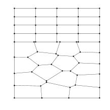
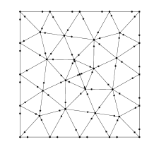
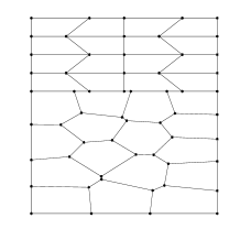
Fig. 1: Sample meshes with small edges. From left to right: $\mathcal{T}_{h}^{1}$, $\mathcal{T}_{h}^{2}$ for $N=4$ and $\mathcal{T}_{h}^{3}$ for $N=4$.

6.1 The load problem

On this test our interest is to approximate the solution of (2.1) for a given load $f\in H^{1}(\Omega)$. The aim of this test is to compute error rates in the corresponding norms of the problem. In this test, we consider two scenarios: the first one is considering the coefficient $\kappa(\mathbf{x})$ constant in the whole domain $\Omega$ and hence, piecewise constant on each polygon of the mesh, whereas in the second we consider $\kappa(\mathbf{x})$ beyond our developed theory, where this coefficient is a bounded function. In both tests, the domain in which we state problem (1.1) is the unit square $\Omega:=(0,1)^{2}$ with null Dirichlet boundary condition on $\partial\Omega$.

6.1.1 Piecewise constant $\kappa(\mathbf{x})$

Here, the value of $\kappa(\mathbf{x})=1=\gamma(\mathbf{x})$, for all $\mathbf{x}\in\Omega$ and $\mathbf{\vartheta}(\mathbf{x}):=(x,y)^{\texttt{t}}$. The load $f$ and Dirichlet boundary conditions are chosen in such a way that the exact solution is $u(\mathbf{x}):=\sin(\pi x)\sin(\pi y).$

In Figure 2 we show, in log-log scale, the error convergence curves in $L^{2}$ and $H^{1}$ between the solution $u$ and the polynomial projection of the virtual solution $u_{h}$.

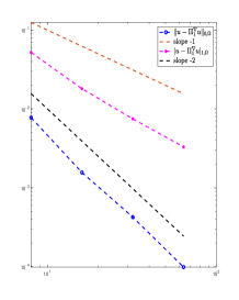
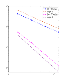
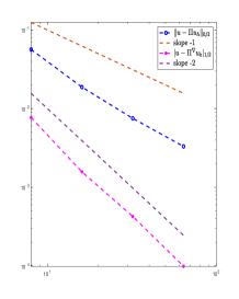
Fig. 2: Test 1: $L^{2}$ error with seminorm $H^{1}$ error for $\mathcal{T}_{h}^{1}$ (left), $\mathcal{T}_{h}^{2}$ (middle)and $\mathcal{T}_{h}^{3}$ (right).

We observe from Figure 2 a clear quadratic order of convergence for error in $L^{2}$ and order 1 for the seminorm. Note that this is the optimal order, as demonstrated in the theoretical section.

6.1.2 Bounded and smooth $\kappa(\mathbf{x})$

In this test, we consider the following functions

$$\kappa(\mathbf{x}):=1,\qquad\mathbf{\vartheta}(\mathbf{x}):=\left(\begin{array}[]{c}x\\ y\end{array}\right),\qquad\text{ and }\qquad\gamma(\mathbf{x}):=x^{2}+y^{3},$$

and with right-hand side and Dirichlet boundary conditions defined in such a way that the exact solution is

$$u(\mathbf{x}):=(x-x^{2})(y-y^{2})+\sin(2\pi x)\sin(2\pi y).$$

Let us remark that the present test goes beyond of the developed theory, since for all the calculations hold, the hypothesis on the coefficients is that all of the must be piecewise constant on each polygon, which in Test 1 hold. However, the method is robust independently of this assumption. In Figure 3 we observe precisely what we claim, where the error decreases for each of the meshes considered.

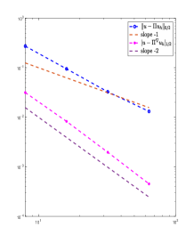
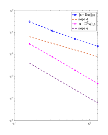
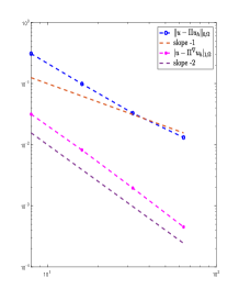
Fig. 3: Test 2: $L^{2}$ error with seminorm 1 error for $\mathcal{T}_{h}^{1}$ (left), $\mathcal{T}_{h}^{2}$ (middle)and $\mathcal{T}_{h}^{3}$ (right).

6.2 The eigenvalue problem

Now our task is to approximate the eigenvalues and eigenfunctions of problem (5.1) with our small edges approach. For this test we consider two scenarios: a convex and a non-convex domain. The order of convergence is computed with a least-square fitting.

6.2.1 Unitary square

Let us consider as computational domain the unit square $\Omega:=(0,1)^{2}$. This domain is discretized with meshes presented in Figure 1. The analytical solution to the convection-diffusion spectral problem is as follows (see [31])

$$\lambda_{p,q} =\dfrac{|\mathbf{\vartheta}|^{2}}{4\kappa}+\kappa\pi^{2}(p^{2}+q^{2})=\lambda_{p,q}^{*}\qquad\text{for }p,q\in\mathbb{N}_{+},$$

$$u_{p,q}(x,y) =\exp\left(\dfrac{\mathbf{\vartheta}\cdot(x,y)}{2\kappa}\right)\sin(p\pi x)\sin(q\pi y),$$ (6.1)

$$u_{p,q}^{*}(x,y) =\exp\left(-\dfrac{\mathbf{\vartheta}\cdot(x,y)}{2\kappa}\right)\sin(p\pi x)\sin(q\pi y).$$ (6.2)

For this test, we have used $\mathbf{\vartheta}(\mathbf{x})=(1,0)^{t}$ and $\kappa(\mathbf{x})=1$. In Table 1, we report the first six eigenvalues computed with meshes $\mathcal{T}_{h}^{2}$ and $\mathcal{T}_{h}^{3}$. The row “Order” reports the convergence order of the eigenvalues, computed with respect to the exact ones obtained with (6.2), which are presented in the row “Exact”.

Table 1: Test 1. The lowest computed eigenvalues $\lambda_{h}^{(i)}$, $1\leq i\leq 6$ for different meshes.

$\mathcal{T}_{h}^{1}$
$N$	$\lambda_{h}^{(1)}$	$\lambda_{h}^{(2)}$	$\lambda_{h}^{(3)}$	$\lambda_{h}^{(4)}$	$\lambda_{h}^{(5)}$	$\lambda_{h}^{(6)}$
8	20.8691	52.3774	57.8481	93.6945	106.3515	134.1838
16	20.1847	51.5506	50.2396	82.4563	100.6677	107.8481
32	20.0379	50.0865	49.7503	79.9785	99.3560	101.1318
64	20.0010	49.6345	49.7195	79.3947	99.0459	99.5049
Order	2.08	2.08	2.03	2.09	2.07	2.00
Exact	19.9892	49.5980	49.5980	79.2068	98.9460	98.9460
$\mathcal{T}_{h}^{2}$
$N$	$\lambda_{h}^{(1)}$	$\lambda_{h}^{(2)}$	$\lambda_{h}^{(3)}$	$\lambda_{h}^{(4)}$	$\lambda_{h}^{(5)}$	$\lambda_{h}^{(6)}$
8	20.8967	56.0401	56.1475	96.3325	125.4921	125.0578
16	20.2310	51.1774	51.1054	83.2877	105.0248	105.2693
32	20.0531	49.9872	49.9944	80.2748	100.5110	100.5074
64	20.0057	49.7015	49.7027	79.4760	99.3675	99.359
Order	1.93	1.99	1.98	1.99	1.99	1.99
Exact	19.9892	49.5980	49.5980	79.2068	98.9460	98.9460
$\mathcal{T}_{h}^{3}$
$N$	$\lambda_{h}^{(1)}$	$\lambda_{h}^{(2)}$	$\lambda_{h}^{(3)}$	$\lambda_{h}^{(4)}$	$\lambda_{h}^{(5)}$	$\lambda_{h}^{(6)}$
8	20.8669	58.1517	52.3612	94.0519	106.2181	137.1134
16	20.1847	51.5743	50.2385	82.4877	100.6575	108.0124
32	20.0379	50.0877	49.7502	79.9805	99.3554	101.1401
64	20.0010	49.7196	49.6345	79.3948	99.0459	99.5054
Order	2.07	2.04	2.08	2.10	2.06	2.03
Exact	19.9892	49.5980	49.5980	79.2068	98.9460	98.9460

We observe from the reported results that for all meshes, the eigenvalues converge with order $\mathcal{O}(h^{2})$. Despite to the fact that the problem is non symmetric, the computed eigenvalues are all real. On the other hand, the eigenvalues converge to the exact eigenvalues that we show in the row ”Exact”.

To end this test, in Figure 4 we present plots of the first, second and four eigenfunctions of our problem.

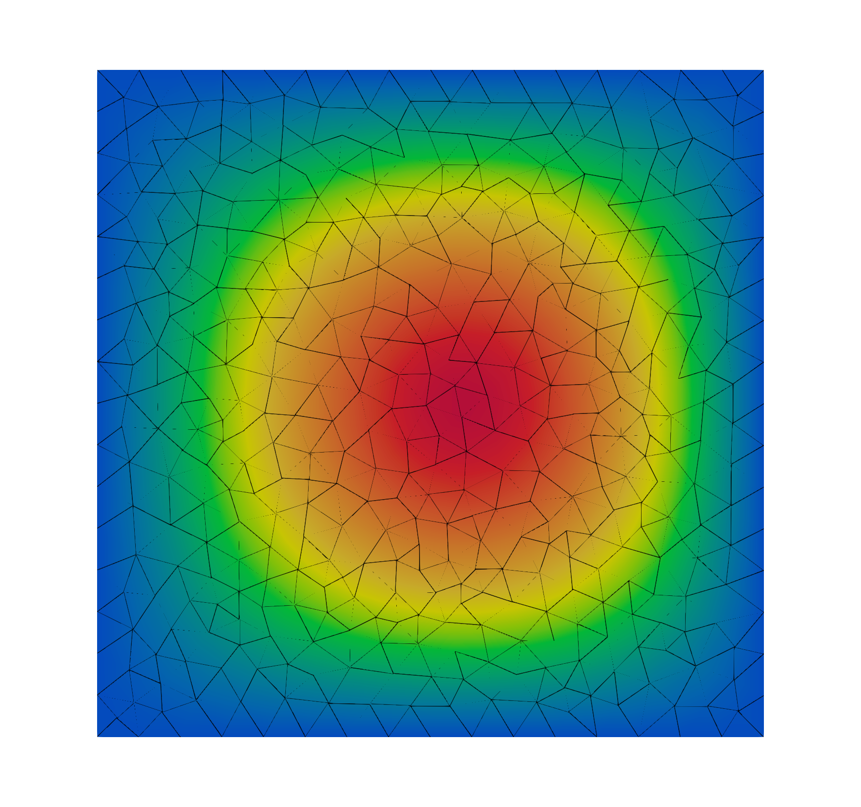
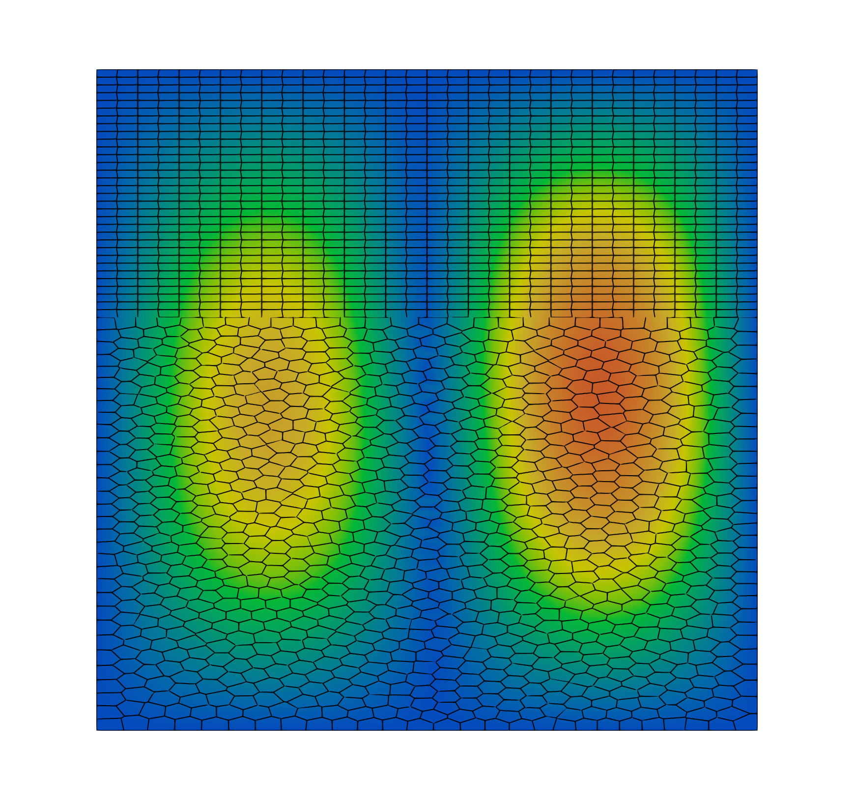
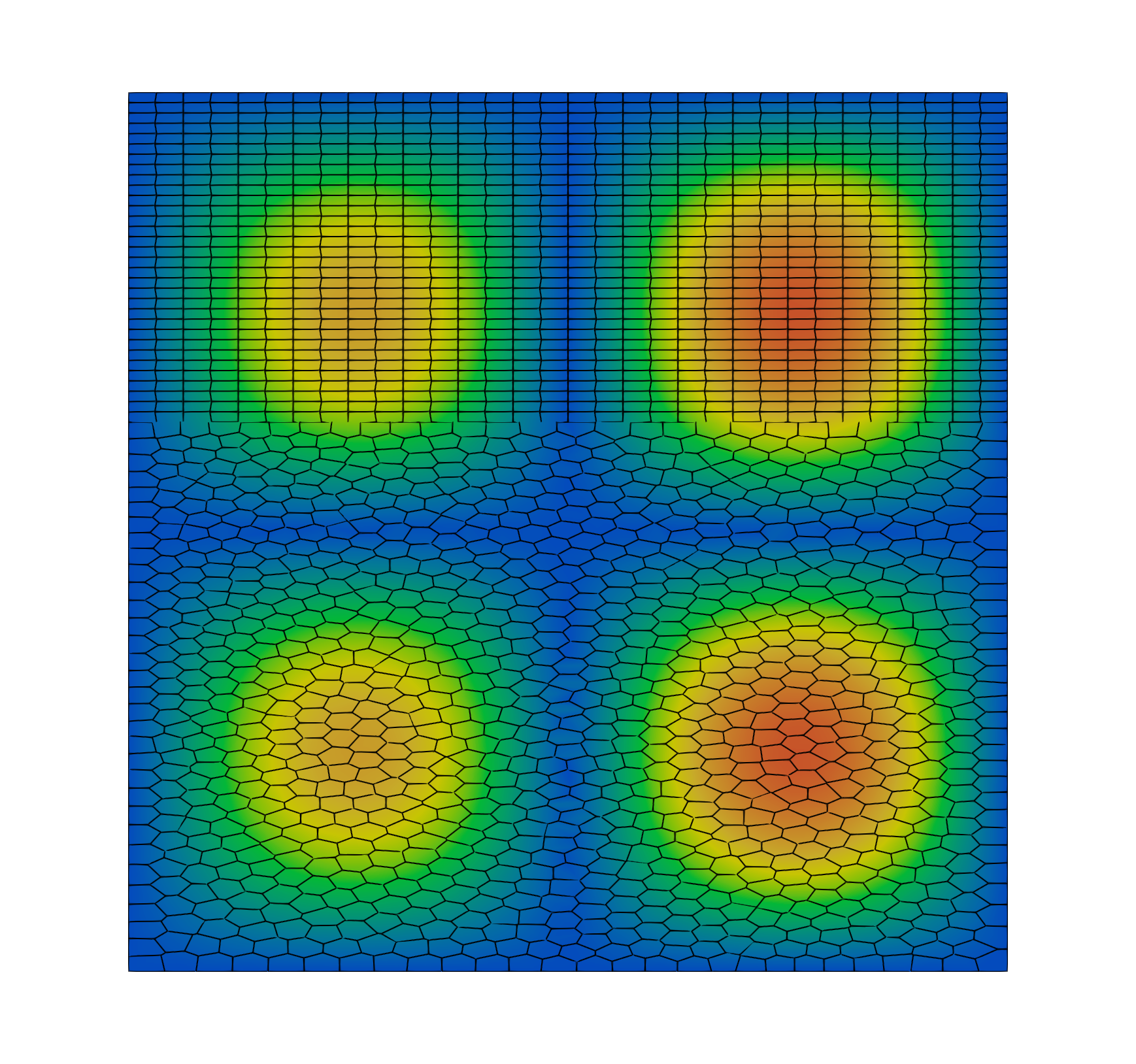
Fig. 4: From left to right, plots of the first, second and four eigenfunctions, computed with $\mathcal{T}_{h}^{2}$ and $\mathcal{T}_{h}^{3}$.

6.2.2 Non convex domain

In the following test we will consider a non-convex domain which we call rotated T, and it is defined by $\Omega:=(-0.5,0.5)\times(-0.5,0)\cup(-0.25,0.25)\times(0,1)$ with boundary condition $u=0$ on the whole boundary $\partial\Omega$. This non-convex domain presents two reentrant angles of the same size $\omega=3\pi/2$ (cf. Figure 5), and as a consequence, the eigenfunctions of this problem may present singularities.

In Figure 5, we present the meshes that we will consider for this numerical test. We note that the families of polygonal meshes $\mathcal{T}_{h}^{3}$, $\mathcal{T}_{h}^{4}$ and $\mathcal{T}_{h}^{5}$ have been obtained by gluing two different polygonal meshes at $x=0$. It can be seen that very small edges compared with the element diameter appears on the interface of the resulting meshes.

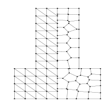
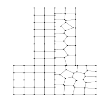
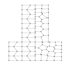
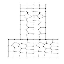
Fig. 5: Sample meshes with small edges. From top left to bottom right: $\mathcal{T}_{h}^{4}$, $\mathcal{T}_{h}^{5}$, $\mathcal{T}_{h}^{6}$ and $\mathcal{T}_{h}^{7}$, for $N=8$.

In Table 2 we report the first six computed eigenvalues with our method. We claim that for this geometry we do not have analytical solution. Hence, we compare our results with extrapolated values that we present in the row ”Extrap”. As in the previous example, the order of convergence, reported in the row ”Order” have been computed with a least-square fitting.

Table 2: Test 1. The lowest computed eigenvalues $\lambda_{h}^{(i)}$, $1\leq i\leq 6$ for different meshes.

$\mathcal{T}_{h}^{4}$
$N$	$\lambda_{h}^{(1)}$	$\lambda_{h}^{(2)}$	$\lambda_{h}^{(3)}$	$\lambda_{h}^{(4)}$	$\lambda_{h}^{(5)}$	$\lambda_{h}^{(6)}$
16	35.8647	50.9369	74.3495	79.8639	107.1151	138.1449
30	34.9179	49.8908	72.0953	76.7690	102.5379	130.5160
62	34.5028	49.6345	71.5289	75.8149	101.3815	128.6860
130	34.3804	49.5724	71.3967	75.5511	101.0999	128.2229
Order	1.50	2.28	2.25	1.95	2.24	2.09
Extrap.	34.3074	49.5656	71.3771	75.4885	101.0644	127.9790
$\mathcal{T}_{h}^{5}$
$N$	$\lambda_{h}^{(1)}$	$\lambda_{h}^{(2)}$	$\lambda_{h}^{(3)}$	$\lambda_{h}^{(4)}$	$\lambda_{h}^{(5)}$	$\lambda_{h}^{(6)}$
16	36.1795	51.3140	75.4220	81.3284	109.2599	141.7893
30	35.0277	49.9852	72.3584	77.1608	103.0639	131.3561
62	34.5422	49.6585	71.5953	75.9265	101.5153	128.8964
130	34.3950	49.5786	71.4136	75.5848	101.1348	128.2769
Order	1.54	2.27	2.26	2.00	2.25	2.32
Extrap.	34.3172	49.5695	71.3900	75.5147	101.0894	128.2296
$\mathcal{T}_{h}^{6}$
$N$	$\lambda_{h}^{(1)}$	$\lambda_{h}^{(2)}$	$\lambda_{h}^{(3)}$	$\lambda_{h}^{(4)}$	$\lambda_{h}^{(5)}$	$\lambda_{h}^{(6)}$
16	36.1709	51.3411	75.4263	81.3049	109.2335	141.8461
30	35.0258	49.9870	72.3587	77.1569	103.0624	131.3610
62	34.5418	49.6586	71.5954	75.9258	101.5152	128.8966
130	34.3949	49.5786	71.4136	75.5846	101.1348	128.2769
Order	1.54	2.29	2.26	1.99	2.24	2.33
Extrap.	34.3180	49.5702	71.3897	75.5101	101.0851	128.2359
$\mathcal{T}_{h}^{7}$
$N$	$\lambda_{h}^{(1)}$	$\lambda_{h}^{(2)}$	$\lambda_{h}^{(3)}$	$\lambda_{h}^{(4)}$	$\lambda_{h}^{(5)}$	$\lambda_{h}^{(6)}$
16	36.1532	51.2579	75.0659	80.8267	108.4547	140.4589
28	35.0908	49.9516	72.2464	77.0487	102.8661	130.9399
60	34.5461	49.6508	71.5580	75.8867	101.4574	128.7725
132	34.3937	49.5760	71.4041	75.5698	101.1188	128.2443
Order	1.56	2.69	2.62	2.23	2.56	2.71
Extrap.	34.3209	49.5847	71.4127	75.5577	101.1394	128.3053

From Table 2 it is possible to observe the effects of the singularities of the domain on the computed order of convergence for the first eigenvalue. Clearly the eigenfunction associated to this eigenvalue is non smooth, which precisely affects the order of convergence. We remark that this phenomenon occurs for each of the meshes considered for this test. On the other hand, the rest of the computed eigenvalues converge to the extrapolated values with order $\mathcal{O}(h^{2})$ as is expected.

Once again, the computed eigenvalues for this test are real and no complex eigenvalues have been observed. We end our test presenting plots for the first four eigenfunctions of the spectral problem in Figure 6.

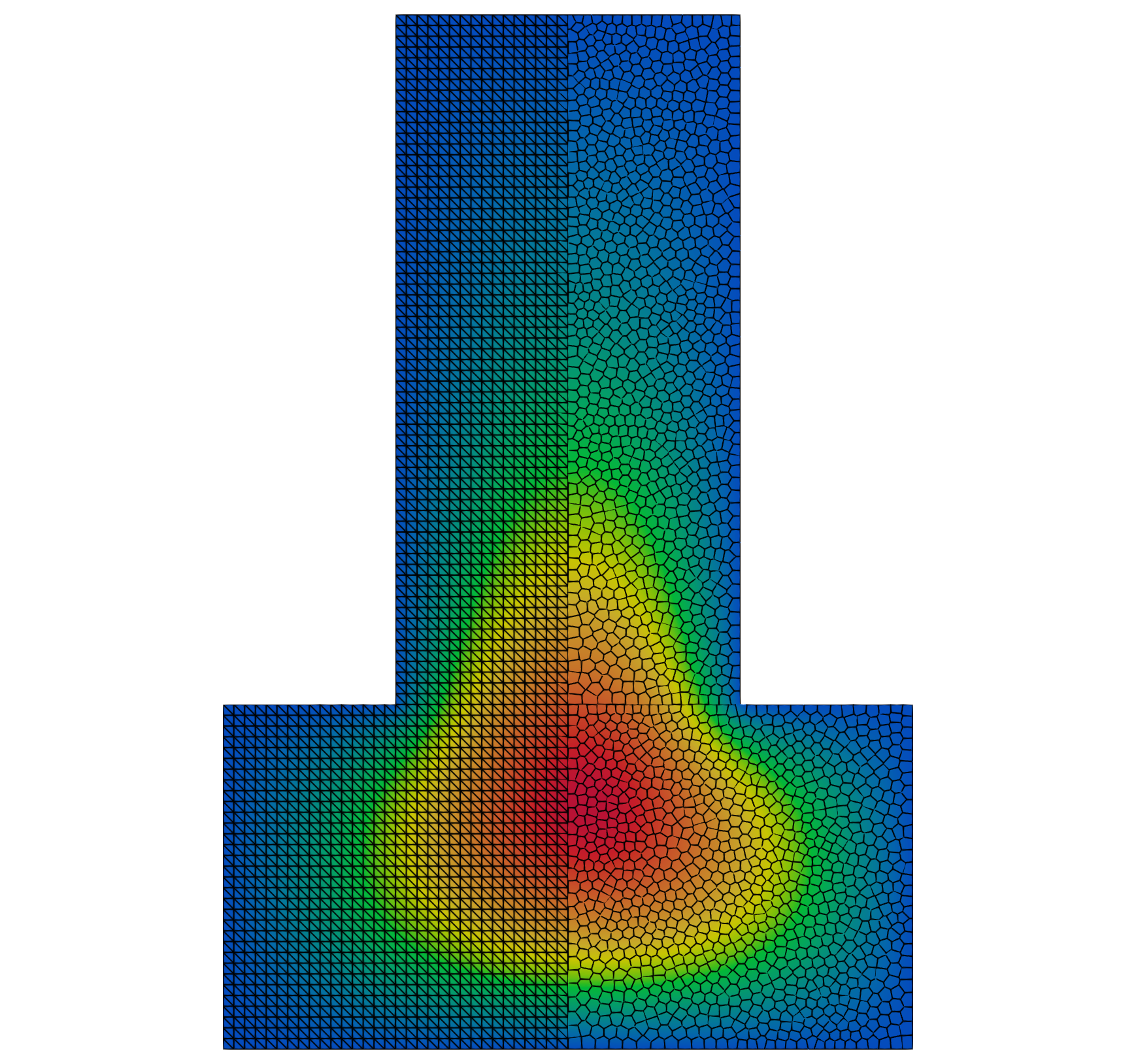
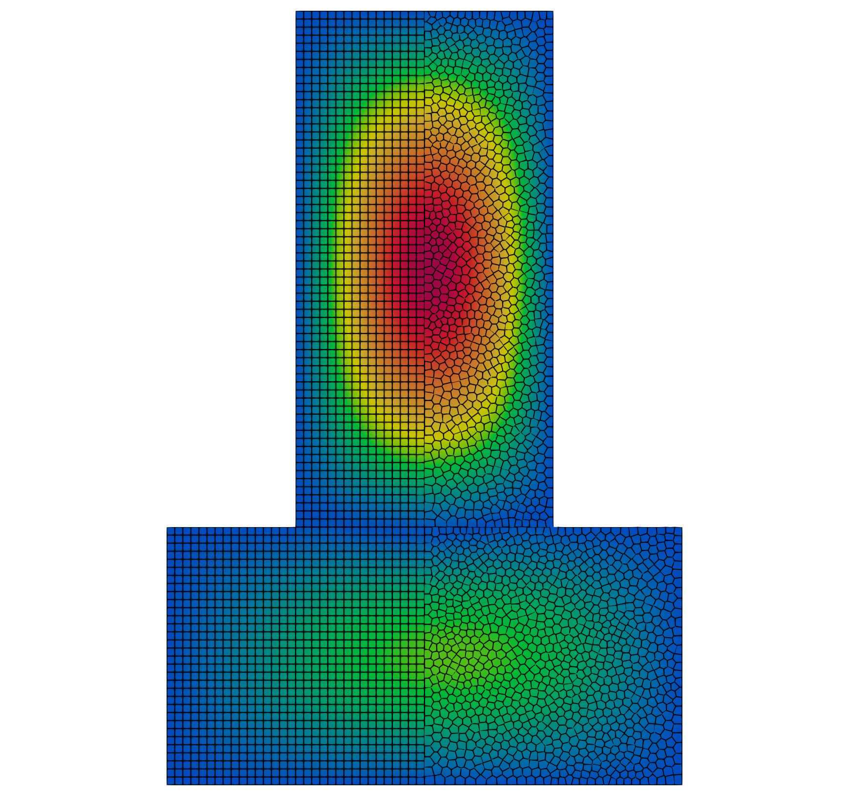
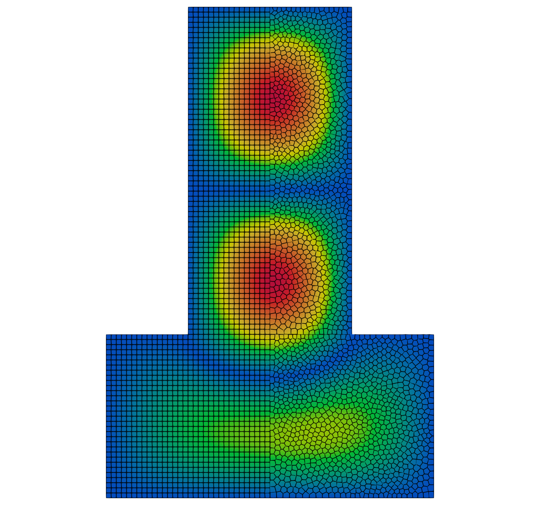
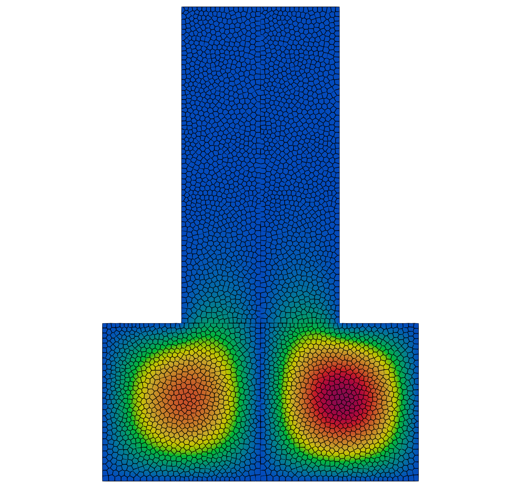
Fig. 6: From top left to bottom right, plots of the first four eigenfunctions for the rotated T domain, computed with $\mathcal{T}_{h}^{4}$, $\mathcal{T}_{h}^{5}$, $\mathcal{T}_{h}^{6}$ and $\mathcal{T}_{h}^{7}$, respectively.

References

• [1] D. Adak, G. Manzini, and S. Natarajan, Virtual element approximation of two-dimensional parabolic variational inequalities, Comput. Math. Appl., 116 (2022), pp. 48–70.
• [2] B. Ahmad, A. Alsaedi, F. Brezzi, L. D. Marini, and A. Russo, Equivalent projectors for virtual element methods, Comput. Math. Appl., 66 (2013), pp. 376–391.
• [3] D. Amigo, F. Lepe, and G. Rivera, A virtual element method for the elasticity problem allowing small edges, arXiv:2211.02792, (2022).
• [4] P. F. Antonietti, L. Beirão da Veiga, and G. Manzini, The Virtual Element Method and its Applications, vol. 31, SEMA SIMAI Springer Series, 2022.
• [5] P. F. Antonietti, L. Beirão da Veiga, D. Mora, and M. Verani, A stream virtual element formulation of the Stokes problem on polygonal meshes, SIAM J. Numer. Anal., 52 (2014), pp. 386–404.
• [6] P. F. Antonietti, L. Beirão da Veiga, S. Scacchi, and M. Verani, A $C^{1}$ virtual element method for the Cahn-Hilliard equation with polygonal meshes, SIAM J. Numer. Anal., 54 (2016), pp. 34–56.
• [7] E. Artioli, S. de Miranda, C. Lovadina, and L. Patruno, A family of virtual element methods for plane elasticity problems based on the Hellinger-Reissner principle, Comput. Methods Appl. Mech. Engrg., 340 (2018), pp. 978–999.
• [8] I. Babuška and J. Osborn, Eigenvalue problems, Handb. Numer. Anal., II, North-Holland, Amsterdam, 1991.
• [9] L. Beirão da Veiga, F. Brezzi, A. Cangiani, G. Manzini, L. D. Marini, and A. Russo, Basic principles of virtual element methods, Math. Models Methods Appl. Sci., 23 (2013), pp. 199–214.
• [10] L. Beirão da Veiga, F. Brezzi, F. Dassi, L. D. Marini, and A. Russo, Virtual element approximation of 2D magnetostatic problems, Comput. Methods Appl. Mech. Engrg., 327 (2017), pp. 173–195.
• [11] L. Beirão da Veiga, F. Brezzi, and L. D. Marini, Virtual elements for linear elasticity problems, SIAM J. Numer. Anal., 51 (2013), pp. 794–812.
• [12] L. Beirão da Veiga, F. Brezzi, L. D. Marini, and A. Russo, Virtual element method for general second-order elliptic problems on polygonal meshes, Math. Models Methods Appl. Sci., 26 (2016), pp. 729–750.
• [13] L. Beirão da Veiga, C. Lovadina, and A. Russo, Stability analysis for the virtual element method, Math. Models Methods Appl. Sci., 27 (2017), pp. 2557–2594.
• [14] D. Boffi, Finite element approximation of eigenvalue problems, Acta Numer., 19 (2010), pp. 1–120.
• [15] S. C. Brenner and L. R. Scott, The Mathematical Theory of Finite Element Methods, Springer, New York, 2008.
• [16] S. C. Brenner and L.Y. Sung, Virtual element methods on meshes with small edges or faces, Math. Models Methods Appl. Sci., 28 (2018), pp. 1291–1336.
• [17] E. Cáceres and G. N. Gatica, A mixed virtual element method for the pseudostress-velocity formulation of the Stokes problem, IMA J. Numer. Anal., 37 (2017), pp. 296–331.
• [18] A. Cangiani, E. H. Georgoulis, T. Pryer, and O. J. Sutton, A posteriori error estimates for the virtual element method, Numer. Math., 137 (2017), pp. 857–893.
• [19] C. Carstensen, J. Gedicke, V. Mehrmann, and A. Miedlar, An adaptive homotopy approach for non-selfadjoint eigenvalue problems, Numer. Math., 119 (2011), pp. 557–583.
• [20] J. Droniou and L. Yemm, Robust hybrid high-order method on polytopal meshes with small faces, Comput. Methods Appl. Math., 22 (2022), pp. 47–71.
• [21] M. Frittelli and I. Sgura, Virtual element method for the Laplace-Beltrami equation on surfaces, ESAIM Math. Model. Numer. Anal., 52 (2018), pp. 965–993.
• [22] F. Gardini, G. Manzini, and G. Vacca, The nonconforming virtual element method for eigenvalue problems, ESAIM Math. Model. Numer. Anal., 53 (2019), pp. 749–774.
• [23] F. Gardini and G. Vacca, Virtual element method for second-order elliptic eigenvalue problems, IMA J. Numer. Anal., 38 (2018), pp. 2026–2054.
• [24] J. Gedicke and C. Carstensen, A posteriori error estimators for convection-diffusion eigenvalue problems, Comput. Methods Appl. Mech. Engrg., 268 (2014), pp. 160–177.
• [25] Vivette Girault and Pierre-Arnaud Raviart, Finite element methods for Navier-Stokes equations, vol. 5 of Springer Series in Computational Mathematics, Springer-Verlag, Berlin, 1986. Theory and algorithms.
• [26] T. Kato, Perturbation theory for linear operators, Die Grundlehren der mathematischen Wissenschaften, Band 132, Springer-Verlag New York, Inc., New York, 1966.
• [27] F. Lepe, D. Mora, G. Rivera, and I. Velásquez, A virtual element method for the Steklov eigenvalue problem allowing small edges, J. Sci. Comput., 88 (2021), pp. Paper No. 44, 21.
• [28] F. Lepe and G. Rivera, A priori error analysis for a mixed VEM discretization of the spectral problem for the Laplacian operator, Calcolo, 58 (2021), pp. Paper No. 20, 30.
• [29]  , A virtual element approximation for the pseudostress formulation of the Stokes eigenvalue problem, Comput. Methods Appl. Mech. Engrg., 379 (2021), pp. Paper No. 113753, 21.
• [30] D. Mora, G. Rivera, and R. Rodríguez, A virtual element method for the Steklov eigenvalue problem, Math. Models Methods Appl. Sci., 25 (2015), pp. 1421–1445.
• [31] A. Naga and Z. Zhang, Function value recovery and its application in eigenvalue problems, SIAM J. Numer. Anal., 50 (2012), pp. 272–286.
• [32] J. Tushar, A. Kumar, and S. Kumar, Virtual element methods for general linear elliptic interface problems on polygonal meshes with small edges, Comput. Math. Appl., 122 (2022), pp. 61–75.
• [33] P. Wriggers, W. T. Rust, and B. D. Reddy, A virtual element method for contact, Comput. Mech., 58 (2016), pp. 1039–1050.