Conformalized semi-supervised random forest for classification and abnormality detection

Abstract

Traditional classifiers infer labels under the premise that the training and test samples are generated from the same distribution. This assumption can be problematic for safety-critical applications such as medical diagnosis and network attack detection. In this paper, we consider the multi-class classification problem when the training data and the test data may have different distributions. We propose conformalized semi-supervised random forest (CSForest), which constructs set-valued predictions $C(x)$ to include the correct class label with desired probability while detecting outliers efficiently. We compare the proposed method to other state-of-art methods in both a synthetic example and a real data application to demonstrate the strength of our proposal.

1 Introduction

A classifier usually makes predictions for a test sample by selecting the class label with the highest predicted probability. Such a strategy is insufficient to meet the growing interest in characterizing the prediction reliability in real applications such as medical diagnosis Esteva et al. (2017); Kompa et al. (2021) and autonomous vehicles Kalra & Paddock (2016); Qayyum et al. (2020). To address this need, we can minimize a mixed cost on miss-classification and rejection to allow refraining from making any prediction on a test sample with high uncertainty. For instance, we may refrain from predicting an observation $x$ with small $\max_{k\in\{0,1\}}\hat{p}_{k}(x)$ for the binary response, where $\hat{p}_{k}(x)$ is the estimated probability using the training data for being class $k$ at observation $x$ Chow (1970); Herbei & Wegkamp (2006); Bartlett & Wegkamp (2008). This idea has been applied to different learning algorithms and extended to the multi-class classification problem Cortes et al. (2016); Ni et al. (2019); Charoenphakdee et al. (2021). Alternatively, another line of work adopts the set-valued prediction framework where the classifier outputs all plausible labels at $x$ using the estimated probabilities $\hat{p}_{k}(x)$. For example, one may construct $\hat{C}(x)=\{k:\hat{p}_{k}(x)\geq\tau_{k}\}$ with $\tau_{k}$ selected to guarantee a desired coverage of the true label Vovk et al. (2005).

Despite such progress, the work above assumes that the training and test samples are i.i.d generated from the same distribution, with the rejection rules capturing uncertain areas in the training cohort. However, it is crucial to characterize uncertainty under distributional changes in many safety-critical systems and flag alerting test samples where we should not trust the model trained with the training set. For example, in medical applications, the test cohort may contain samples that represent novel pathology and bear low similarity to labeled training set (Lin et al., 2005). Also, network attackers may generate novel intrusions to circumvent current detection systems (Marchette & Marchette, 2001).

In this paper, we propose CSForest (Conformalized Semi-supervised random Forest) for calibrated set-valued prediction under the non-iid setting where the training and test cohort can have disparity. The proposed method constructs a semi-supervised random forest ensemble with both labeled training data and unlabeled test data and adapts the idea of Jacknife+aB to accompany this semi-supervised ensemble with well-calibrated prediction interval (Kim et al., 2020). CSForest achieves significantly better classification accuracy than existing classification methods while providing a provable worst-case coverage guarantee on the true labels in our numerical experiments. We give a glimpse of its strength over alternative methods in section 1.1.

1.1 Preview of CSForest

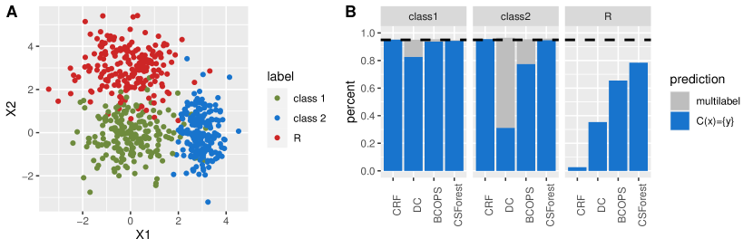
Figure 1: FIG1A shows the first two dimensions of samples are generated from the three classes: green/blue/red points representing samples from class 1/2/R. FIG1B shows the coverage rate which is defined by the proportion of samples with true labels included in their prediction sets. The horizontal dash line refers to the coverage level of 95%. FIG1B is grouped by the actual labels in the testing data and colored based on if a prediction set contains only the correct label (blue) or more than correct label (gray).

Before we proceed to the details of CSForest, we first compare it with BCOPS (Balanced&Conformalized Optimal Prediction Sets) and CRF (Comformalized Random Forest) and DC (Density-set Classifier) on a simulated classification task described in Example 1. BCOPS, CRF and DC represent three different types of calibrated set-valued prediction.

• BCOPS combines a semi-supervised classifier separating different training classes and the unlabeled test cohort and constructs a calibrated set-valued prediction using sample-splitting conformal prediction (Guan & Tibshirani, 2022). Compared to CSForest, BCOPS utilizes poorly both the training samples and the test samples. We will provide more details in section 2 and section 3. In this paper, we used random forest (Breiman, 2001) as the classifier in BCOPS.

• CRF constructs the set-valued prediction $\{k:\hat{p}_{k}(x)\geq\tau_{k}\}$ by including training labels $k$ achieving high estimated probability from the random forest classifier, with the cut-offs $\tau_{k}$ chosen based on sample-splitting conformal prediction Vovk et al. (2005).

• DC constructs the set-valued prediction similarly to CRF, except for replacing the estimated probability $\hat{p}_{k}(x)$ by an estimation of the density function for class $k$ using the training data Hechtlinger et al. (2018).

Example 1.

Let $X\in^{10}$ be a ten-dimensional feature. In the training data, we observe two classes $Y\in\{1,2\}$, but the test data contains a novel component labeled with $Y=R$. For each component, $X_{j}\sim N(0,1)$ $(j=3,\ldots,10)$ are noise, with different components separated by the first two dimensions:

$$\left\{\begin{aligned} &X_{1}\sim N(0,1),\;X_{2}\sim N(0,1),\quad Y=1,\\ &X_{1}\sim N(3,0.5),\;X_{2}\sim N(0,1),\quad Y=2,\\ &X_{1}\sim N(0,1),\;X_{2}\sim N(3,1),\quad Y=R.\end{aligned}\right.$$

FIG1A shows the first two dimensions of samples generated from the three classes $Y\in\{1,2,R\}$. We generate 200 samples from class 1 and class 2 to form the training set and 200 samples from each of the three classes to form the test set.

We evaluate the performance by type I error and type II error. Type I error is defined as the percentage of samples with true label excluded from its associated set-valued prediction $\hat{C}(x)$ for observed classes. Type II error is constructed as the percentage of samples with $\hat{C}(x)$ containing labels other than the true labels.

In FIG1B, we evaluated the quality of the set-valued prediction $\hat{C}(x)$ using DC, CRF, BCOPS and CSForest across 20 independent runs with a targeted miscoverage rate at $\alpha=0.05$. All four methods have been calibrated using conformal prediction and achieve the desired coverage on true labels. However, CSForest and BCOPS are both adaptive to the test cohort and improve over CRF and DC for outlier detection by a large margin. In addition, compared to BCOPS, CSForest has fewer samples with multiple labels from class $1$ and $2$ (higher specificity/low type II error), and has a higher percent of rejection on outliers which is equivalent to smaller type II error in the outlier class.

2 Related work

Conformal prediction with different splitting schemes. Split conformal prediction offers an easy-to-implement but reliable recipe for capturing the prediction uncertainty (Vovk et al., 2005). It first splits the training sample pairs $(X_{i},Y_{i})$ into two sets $\mathcal{I}_{tr}^{1}$ and $\mathcal{I}_{tr}^{2}$. Then, it uses $\mathcal{I}_{tr}^{1}$ to learn a score function $\hat{s}(x,y):^{p+1}\mapsto$ and $\mathcal{I}_{tr}^{2}$ to make a calibrated decision about whether to include a particular choice of $y$ in the prediction set:

$$\hat{C}(x)=\{y:\frac{\left(1+\sum_{(x_{i},y_{i})\in\mathcal{I}_{tr}^{2}}\mathbbm{1}_{\hat{s}(x,y)\geq\hat{s}(x_{i},y_{i})}\right)}{|\mathcal{I}_{tr}^{2}|+1}\geq\alpha.\}$$

The constructed $\hat{C}(x)$ covers the unobserved $Y_{n+1}$ of the test sample $X_{n+1}$ with guaranteed probability $(1-\alpha)$, given that the training samples and that the test sample $(X_{n+1},Y_{n+1})$ are exchangeable with each other.

In Vovk et al. (2018), the authors proposed the cross-conformal prediction method to improve the data utilization efficiency, which calculates scores for each fold of data using score functions learned from the remaining folds. Barber et al. (2021) further proposed Jacknife+ for regression problems that combine Jacknife with conformal prediction and constructed the prediction interval as

$$\hat{C}(x)=\left\{y:\frac{1}{n+1}\left(1+\sum_{i=1}^{n}\mathbbm{1}_{\hat{s}^{i}(x,y)\geq\hat{s}^{i}(x_{i},y_{i})}\right)\geq\alpha\right\},$$

where $\hat{s}^{i}(x,y)=|\hat{\mu}^{i}(x)-y|$ is the regression score using the prediction function $\hat{\mu}^{i}(x)$ learned from training samples excluding $(x_{i},y_{i})$. Although Jacknife+ can only provide a worst-case coverage guarantee at level $(1-2\alpha)$, the achieved empirical coverage is often well-calibrated. Jacknife+ tends to offer better construction than the split conformal prediction, with the downside being its computational cost. Kim et al. (2020) described Jacknife+aB to mediate the computational burden, which constructs an ensemble regression score $\hat{s}^{i}(x,y)=|y-\psi(\{\hat{\mu}_{b}(x):i\notin\mathcal{I}^{b}\})|$ where $\hat{\mu}_{b}(x)$ is the estimated prediction function of $y$ using the Bootstrapped training set $\mathcal{I}^{b}$ for $b=1,\ldots,B$, and $\psi(\{\hat{\mu}_{b}(x):i\notin\mathcal{I}^{b}\})$ is an ensemble of all prediction functions $\hat{\mu}_{b}(x)$ with $(x_{i},y_{i})$ excluded from $\mathcal{I}^{b}$.

Generalized label shift model and test-data-adaptive classification. Regarding distributional changes, both the covariate shift model and the label shift model are commonly studied (Schölkopf et al., 2012). The former assumes $p(y|x)$ to be fixed with $p(x)$ potentially changing (Shimodaira, 2000; Bickel et al., 2009; Gretton et al., 2009; Csurka, 2017); the latter treats $p(x|y)$ as fixed, but the prevalence of different labels can vary (Storkey, 2009; Lipton et al., 2018). In both frameworks, the problem of dealing with outliers or novel components is non-trivial. Generalized label shift model in (1) extends the label shift model to include unseen classes, enabling us to deal with outliers conveniently.

Suppose that the training data is a mixture of $K$ different classes. For class $k$, its mixture proportion is $\pi_{k}$, and feature density is $f_{k}(x)$, with $\pi_{k}$ satisfying $\sum_{k=1}^{K}\pi_{k}=1$. The generalized label shift model assumes a target distribution accepting both label shift among training classes and the appearance of outlier component(s) and requires only $f_{k}(x)$ to remain the same for each observed class:

$$\mu(x)=\sum_{k=1}^{K}\tilde{\pi}_{k}f_{k}(x)+\varepsilon\cdot e(x),$$ (1)

where $\varepsilon+\sum_{k=1}^{K}\tilde{\pi}_{k}=1$. Here $\tilde{\pi}_{k}$ represents the proportion of samples from class $k$ in the target distribution, $\varepsilon$ represents the proportion of outlier samples not from the observed classes, and $e(x)$ represents the density for the outlier component.

Under the generalized label shift model, our goal is to construct a set-valued prediction $C(x)$ to include the true label of the observed classes with high probability while avoiding unnecessary false labels in $C(x)$. In other words, given a user-specified true-label inclusion probability $(1-\alpha)$ for each observed class, we aim to minimize the average set length over the target distribution $\mu(x)$.

The BCOPS method aims to optimize the model performance on the test set and sets $\mu(x)=f_{te}(x)$, the marginal density for the test data, and constructs calibrated set-valued prediction combining the empirically estimated $v_{k}(x)$ and the sample-splitting conformal prediction (Vovk et al., 2005). Although BCOPS outperformed non-test-cohort-adaptive approaches for abnormality detection, it relies on the availability of a large set of test data, and the sample-splitting scheme results in low data utilization efficiency Guan & Tibshirani (2022).

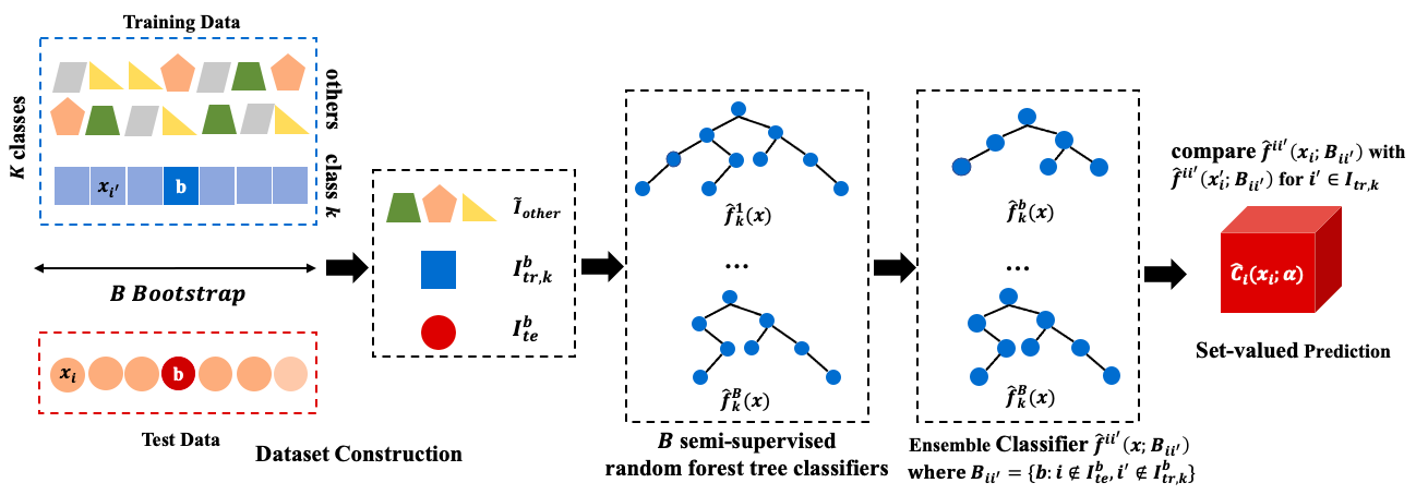
Figure 2: Overview of CSForest Structure.

The main contribution of CSForest is to adapt the idea of Jacknife+aB to the generalized label shift model where we constructed a novel calibrated semi-supervised random forest ensemble for joint multi-class classification and abnormality detection.

Other related alternative strategies: Existing popular approaches for building prediction set $\hat{C}(x)$ in classification problems are often based on $\hat{p}_{k}(x)\coloneqq\hat{p}(k|x)$, the estimated probability of being class $k$ at feature value $x$, using only the training samples. For instance, we could take the point prediction $y=\arg\max_{k}\hat{p}_{tr}(k|x)$. To account for the prediction uncertainty, Vovk et al. (2005) suggested the set-valued prediction $\hat{C}(x)=\{k:\hat{p}_{k}(x)\geq\tau_{k}\}$ with $\tau_{k}$ selected in the combined prediction framework to guarantee a desired coverage of the true label. Later, Romano et al. (2020) considered $\hat{C}(x)=\{k_{(l^{\prime})}:l^{\prime}\leq\min\{l:\sum_{l^{\prime}\leq l}\hat{p}_{k_{(l^{\prime})}}(x)\geq\tau\}\}$ to include $l$ classes label with largest probabilities such that the total probability of $y$ falling into this set sufficiently large. The previous two constructions do not work well with the generalized distributional shift model and abnormality detection in particular. Although we can combine them with the proposal from (Tibshirani et al., 2019) which extends conformal prediction to correctly calibrate the prediction uncertainty in the test samples under the covariate shift model, the modified procedures are sub-optimal under the generalized label shift model for classification as we will demonstrate in our numerical experiments. In (Lei, 2014; Hechtlinger et al., 2018), the authors suggested the use of the density set $\hat{C}(x)=\{k:\hat{p}(x|k)\geq\tau\}$ which outputs an empty set of $\hat{p}(x|k)$ is small for all class $k$. However, $\hat{p}(x|k)$ is often a poor discriminator among the observed classes and insensitive to outliers in high dimensions; consequently, the resulting $\hat{C}(x)$ tends to have a high type II error.

3 Conformalized semi-supervised random forest

We are interested in making set-valued predictions to include true labels frequently but avoid false labels as much as possible for the target distribution $\mu(x)$. More specifically, we consider the following constrained optimization problem:

$$\min\int_{x}|C(x)|\mu(x)dx,$$ (2)

$$s.t.\;\mathbb{P}[k\in C(X)|Y=k]\geq 1-\alpha,$$

$$\mbox{for all }k=1,\ldots,K.$$

CSForest considers optimizing the “average" training and test performance, and considers $\mu(x)=f_{te}(x)+wf_{tr}(x)$ for a weight $w\geq 0$. If $w=0$, $\mu(x)=f_{te}(x)$ and the objective of CSForest coincides with the objective of BCOPS which optimizes for the test cohort classification accuracy. On the other hand, when $w$ is large, it has a similar objective as the CRF model and optimizes more the classification performance on the training set. Proposition 3.1 describes the oracle construction given $\mu(x)$.

Proposition 3.1 (Modified from Proposition 1 in Guan & Tibshirani (2022)).

Set $s_{k}(x;\mu)=[f_{k}(x)/\mu(x)]$. Under the generalized label shift model, the solution to (2) is $C(x)=\{k:\mathbb{E}_{X}[\mathbbm{1}\{s_{k}(x;\mu)\geq s_{k}(X;\mu)\}|Y=k]\geq\alpha,k=1,\ldots,K\}$.

CSForest constructs an empirical version of $C(x)$ via a semi-supervised random forest using the labeled training samples and unlabeled test cohort, coupled with Jacknife+aB strategy for the correct calibration such that the coverage guarantee holds (Kim et al., 2020). It consists of two major components (1) growing a semi-supervised random forest tree separating different training classes and the test samples, (2) comparing how likely a test sample belongs to class $k$ with a sample from training class $k$ using the ensemble prediction on trees excluding these two samples. FIG2 reveals the model structure of CSForest. The second component adapts Jacknife+aB strategy where we need to exclude the paired training-test observations when performing the comparison, rather than excluding a single training sample in Jacknife+aB.

Let $\mathcal{I}_{tr}$ and $\mathcal{I}_{te}$ denote the training and the test sets. Let $\mathcal{I}_{tr,k}$ denote samples from training class $k$ with size $n_{k}$. Algorithm 1 gives details for CSForest: (1) Line 2-5 constructs $B$ semi-supervised random forest tree classifiers, (2) Line 6 constructs the ensemble classifier $\hat{f}^{ii^{\prime}}(x)$ excluding the paired test and training samples $(i,i^{\prime})$ that measures how likely $x_{i}$ and $x_{i^{\prime}}$ are from class $k$ with $k$ being the class label for the training sample $x_{i^{\prime}}$. Finally, (3) lines 8-13 calibrate the prediction using the ensemble prediction $\hat{f}^{ii^{\prime}}(x)$ for test sample $x_{i}$ and all training samples $i^{\prime}$, and output the calibrated CSForest score $\hat{s}_{ik}$ for each class $k$. Steps (2) and (3) adapt the Jacknife+aB strategy to the semi-supervised random forest classifier and the additional sampling step at line 3 is for the same technical reason in the Jacknife+aB.

Our default choice for $w$ is $w=1$, which is used in all numerical experiments in the main paper including Example 1, where the inliers inform little about the outliers, and vice versa. In Appendix C, we have experimented smaller $w\in[0,1)$ and varying sample sizes to examine if less emphasize on training sample from other classes improves the ability for outlier detection. CSForest is consistently better than BCOPS for $w\in[0,1]$ with $w=1$ a top performer across various settings overall and only slightly worse than $\omega=0$ for outlier detection when the percent of outliers in the pooled training and test cohort is small.

1

Input : Training Data $\{z_{i}\coloneqq(x_{i},y_{i}),i\in\mathcal{I}_{tr}\}$, Test Data $\{(x_{i}),i\in\mathcal{I}_{te}\}$, $\gamma$.

Output : Prediction sets $\hat{C}_{i}(x_{i})$ for $i\in\mathcal{I}_{te}$.

1

2for $k=1,\ldots,K$ do

3       Sample $B$ from ${\rm{Binomial}}(\tilde{B},(1-\frac{1}{n_{k}+1})^{n_{k}})$,

4       for $b=1,\ldots,B$ do

5            

6            Let $\mathcal{I}_{tr,k}^{b}$ and $\mathcal{I}_{te}^{b}$ be the Bootstrap of original data $\mathcal{I}_{tr,k}$ and $\mathcal{I}_{te}$ respectively. Let $\tilde{\mathcal{I}}_{other}$ be the Bootstrap of size $\min(\lceil m\gamma\rceil,n-n_{k})$ from training samples other than class $k$.

7            

8            Grow a single tree random forest classifier $\hat{f}^{b}(x)$ separating different labeled classes and the test samples using $\mathcal{I}_{tr,k}^{b}\cup\mathcal{I}_{te}^{b}\cup\tilde{\mathcal{I}}_{other}$.

9       end for

10      

11      For sample pair $i\in\mathcal{I}_{te},i^{\prime}\in\mathcal{I}_{tr,k}$, set $\mathcal{B}_{ii^{\prime}}=\{b:i\notin\mathcal{I}_{te}^{b},i^{\prime}\notin\mathcal{I}_{tr}^{b,k}\}$ and $\hat{f}^{ii^{\prime}}(x)=\left(\sum_{b\in\mathcal{B}_{ii^{\prime}}}\hat{f}^{b}_{k}(x)\right)/|\mathcal{B}_{ii^{\prime}}|$.

12 end for

13

14for $i\in\mathcal{I}_{te}$ do

15       for $k=1,\ldots,K$ do

16             Construct calibrated score for sample $i$: $\hat{s}_{ik}=\frac{\left(1+\sum_{i^{\prime}\in\mathcal{I}_{tr,k}}\mathbbm{1}\{\hat{f}^{ii^{\prime}}(x_{i})\geq\hat{f}^{ii^{\prime}}(x_{i^{\prime}})\}\right)}{\left(n_{k}+1\right)}$

17       end for

18      Construct prediction set for sample $i$: $\hat{C}_{i}(x)=\left\{k:\hat{s}_{ik}\geq\alpha\right\}$

19 end for

Algorithm 1 Comformalized semi-supervised random forest

In the regression problem where the prediction model is trained on the training cohort, Jacnife+aB provides the worst-case coverage guarantee on the true response at the level $(1-2\alpha)$. Here, we show that CSForest achieves the same level of worst-case coverage guarantee, with achieved empirical coverage close to $(1-\alpha)$ in our experiments.

Theorem 3.2.

Suppose that the generalized label shift model holds where features from class $k$ are i.i.d generated from $\mathcal{P}_{k}$. For any fixed integers $\tilde{B}\geq 1$, the constructed $\hat{C}_{i}(x)$ from CSForest satisfies:

$$\mathbb{P}\left[k\in\hat{C}_{i}(X)|Y=k\right]\geq 1-2\alpha,$$ (3)

$$\mbox{for all }i\in\mathcal{I}_{te}\;\mbox{ and }\;k=1,\ldots,K.$$

The proof for Theorem 3.2 follows from that for Theorem 1 in Kim et al. (2020), with additional arguments needed for including test samples in training (see Appendix A).

4 Numerical Experiments

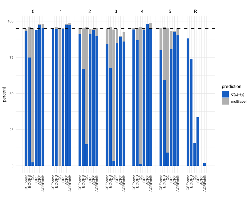
Figure 3: Per-class quality evaluation of all methods with outlier components but no additional label shift among inlier digits. The horizontal dash line refers to the coverage level of 95%. And outliers $R=\{6,7,8,9\}$. FIG3 is grouped by the actual labels in the testing data and colored based on if a prediction set contains only the correct label (blue) or more than the correct label (gray).

In this section, we perform numerical experiments on the MNIST handwritten digit data set, which contains digit labels $Y\in\{0,\ldots,9\}$ with the feature dimension being 784. We compare CSForest to state-of-the-art alternatives, including BCOPS, CRF, DC, as well as the other two approaches achieving adaptive coverage for different classes over the feature space:

• ACRF: We refer to the adaptive-coverage classification approach using random forest proposed in Romano et al. (2020) as ACRFrandom (Adaptive-coverage CRF with randomization) where the randomization is introduced via an additional uniform random variable $U$ for tie-breaking. Here, we consider a non-randomized version of it, referred to as ACRF where we do not use $U$. More specifically, ACRF constructs the prediction set $\hat{C}(x)$ by including labels with large estimated probabilities such that the total probability is greater than $\hat{\tau}_{\alpha}$. Here, $\hat{\tau}_{\alpha}$ is the upper-level quantile of the empirical distribution of $\{E_{i}\}_{i\in\mathcal{I}_{cal}}\cup\{\infty\}$, $\mathcal{I}_{cal}$ is the calibration set in sample-splitting conformal prediction and $E_{i}$ is the sum of estimated probabilities for all labels proceeding that for the true label.

  In this paper, we considered ACRF as one of the baselines instead of ACRFrandom because ACRFrandom sometimes can produce unnecessarily wide prediction set due to trying to achieve the conditional coverage, as pointed out in the original paper Romano et al. (2020), and lead to high type II errors when our goal is only the marginal coverage. We observed this phenomenon in our numerical experiments, which is also confirmed by Romano et al. (2020) for MNIST data using a random forest classifier. More details about ACRF and its comparisons to ACRFrandom are in Appendix B.

• ACRFshift: ACRF suffers from both label shifts of inlier classes and the emergence of outliers. We can combine it with the covariate shift conformal prediction (Tibshirani et al., 2019) to make it more robust, referred to as ACRFshift. Let $r(x)=\frac{\mathbb{P}\{{\rm{test}}|x\}}{\mathbb{P}\{{\rm{train}}|x\}}$ be the odd function for being from the test cohort and $\gamma_{x_{0}}(x)=\frac{r(x)}{r(x_{0})+\sum_{z_{i}\in\mathcal{I}_{cal}}r(x_{i})}$ be the weight function where $x_{0}\in\mathcal{I}_{te}$ and $x\in\mathcal{I}_{cal}$. ACRFshift constructs the prediction set $\hat{C}(x)$ by including labels with large estimated probabilities such that the total probability is greater than $\hat{\tau}_{\alpha}$, where $\hat{\tau}_{\alpha}$ is the upper-level quantile of the weighted empirical distribution on $\{E_{i}\}_{i\in\mathcal{I}_{cal}}\cup\{\infty\}$ with weight $\gamma_{x_{0}}(x_{i})$ for $E_{i}$ and weight $\gamma_{x_{0}}(x_{0})$ for $\infty$. Details of ACRFshift are given in Appendix B.

4.1 Comparisons with no additional label shift

In this experiment, we randomly select 500 samples for each digit 0-5 as the training data and 500 samples for each digit 0-9 as the test data. We then apply BCOPS, DC, CRF, ACRF, ACRF and CSForest. And the set-valued prediction $\hat{C}(x)$ of each method is constructed with $\alpha=0.05$ and $B=3000$ over 10 repetitions. Table 1 shows the average type I and type II errors of different methods on the test data at $\alpha=0.05$. When averaging digits 0-5, all methods achieved the expected coverage, and CSForest has the lowest overall type II error.

Table 1: Achieved Type I and Type II errors at $\alpha=0.05$ with outlier components and no additional label shift among inlier digits. All methods achieved the targeted coverage for inlier digits in this experiment, with CSForest having the lowest type II error because of high specificity across different classes as shown in Figure 3.

Method	Type I Error	Type II Error
CSForest	0.051$\pm$0.005	0.088$\pm$0.008
BCOPS	0.043$\pm$0.004	0.238$\pm$0.019
DC	0.047$\pm$0.008	0.900$\pm$0.021
CRF	0.057$\pm$0.007	0.308$\pm$0.035
ACRF	0.047$\pm$0.006	0.431$\pm$0.003
ACRFshift	0.036$\pm$0.009	0.439$\pm$0.009

FIG3 shows the classification results for different methods via the barplot. ACRF achieves the highest accuracy for inlier digits, followed by CRF and CSForest. However, only CSForest and BCOPS have a good ability to detect outliers digits 6-9, with CSForest achieving a power of more than 89%, followed by BCOPS with a power of slightly less than 75%. Overall, CSForest provides set-valued predictions with quality comparable to CRF for inlier digits but significantly better than all alternatives for abnormality detection among outlier digits. The improved performance of ACRF is due to pursuing a marginal coverage guarantee as opposed to a per-class coverage guarantee when compared to CRF or CSforest, rendering it susceptible to the traditional label shift setting, as we shall see in section 4.3.

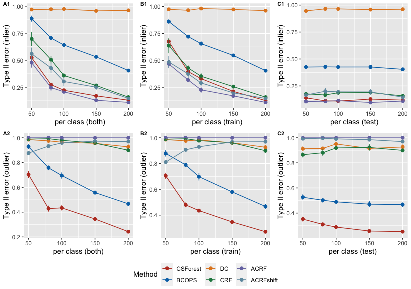
Figure 4: FIG4 Penals A1-C1 show achieved type II error for inliers (digits 0-5) at $\alpha=0.05$ as we vary both per-class training sample size and per-class test sample from 50 to 200, or vary per-class training sample size, or vary per-class test sample size size. Similarly, panels A2-C2 show the achieved type II errors for outliers (digits 6-9) as we vary the sample sizes. It is worth noting that the error bars representing the standard deviation in FIG4 are lower compared to the true standard deviation since the samples are not completely independent.

4.2 Comparisons with varying sample sizes

In this section, we compare different methods under various sample size settings. We vary both the per-class training and test samples from 50 to 200 and compare the type I and type II errors averaged over 10 iterations at $\alpha=0.05$. FIG4 reports the achieved type II error for inliers (digits 0-5) and outliers (digits 6-9) for all models.

From FIG4, while the type II error (inlier) of all methods decreases along with the increase in sample size (with the exception of DC), CSForest and BCOPS are much better at detecting unobserved outlier digits (digits 6-9) compared to others. Furthermore, CSForest achieves the best power for outlier detection while obtaining close to the lowest type II error for inliers as we vary the sample sizes. It is worth noting that the Type II error of ACRFshift on outliers increases as the sample size increases. It is caused by the weights $\gamma_{x_{0}}(x)=\frac{r(x)}{r(x_{0})+\sum_{z_{i}\in\mathcal{I}_{cal}}r(x_{i})}$ which is sensitive to the sample size of the calibration training set $\mathcal{I}_{cal}$ and increases with the training sample size in the sample-splitting scheme.

4.3 Comparisons with additional label shift

In the previous simulations, although we had outliers, the class ratios among inlier classes were balanced and remained the same for training and test cohorts. One nice property for approaches that aim for per-class coverage over approaches that aim for marginal coverage is their robustness against label shift among inlier classes regarding the coverage guarantee. To see this, we now sample data to training and test samples under the traditional label shift model with no outlier digit. We randomly select 500 samples for digits 0-2 and 100 samples for digits 3-5 as the training data. For testing data, we randomly select 100 samples for digits 0-2 and 500 samples for digits 3-5. We repeat each method 10 times with $\alpha=0.05$ and $B=3000$ and calculate the average.

Table 2: Achieved Type I and Type II errors at $\alpha=0.05$ with label shift among inlier digits but no outlier digits. ACRF fails to meet the desired coverage in this setting.

Method	Type I Error	Type II Error
CSForest	0.042$\pm$0.008	0.295$\pm$0.036
BCOPS	0.041$\pm$0.010	0.536$\pm$0.056
DC	0.040$\pm$0.016	0.962$\pm$0.022
CRF	0.036$\pm$0.018	0.523$\pm$0.082
ACRF	0.171$\pm$0.024	0.313$\pm$0.067
ACRFshift	0.080$\pm$0.026	0.630$\pm$0.127

Table 2 shows the achieved type I and type II errors using different methods on this standard label shift simulation. We observed that while CRF, BCOPS and CSForest all achieved desired coverage, ACRF failed due to such distributional changes between training and test cohorts. Although ACRFshift alleviates the under coverage of ACRF, it leads to a much higher type II error compared to CRF and CSForest, highlighting the importance of adopting the right distributional change mechanism in practice. In Appendix B4, we show the coverage barplot for different inlier classes, confirming that the under-coverage of ACRF is due to the over-representation of minority training digits 3-5 in the test cohort, which is severely under-covered using ACRF.

5 Discussion

This paper proposes CSForest as a powerful ensemble classifier to perform robust classification and outlier detection under distributional changes. It aims to construct a set-valued prediction set at each test sample to cover the true label frequently while avoiding false labeling to its best effort. Compared to its precedent BCOPS, CSForest outputs prediction sets of higher quality and is more stable. Although with a worst-case coverage level at $(1-2\alpha)$, the achieved empirical coverage is often close to $(1-\alpha)$ in practice.

How much guidance do we need from the test samples to help us with high-quality outlier detection? While this is data-dependent, when the hidden signal is relatively strong as in the MNIST example, a little guidance makes a big difference. We further consider the setting where we have 200 samples from each class in the train set but only 5 samples from each class in the test set, and examine if the test cohort can guide us toward better outlier detection in this extreme case.

FIG5 shows the achieved type II errors at $\alpha=0.05$ using different methods, separately for inlier and outlier classes. CSForest achieved a type II error of around 42% on average and 60% for outliers with merely five unlabeled samples from outlier digit classes in the test cohort. At the same time, DC has an average type II error of around 95% for this moderately high dimensional example using hundreds of training samples. This suggests that information from the outlier component can be crucial for guiding our decision in detecting outliers in high dimensions. We can be much more effective in discriminating outliers from normal classes if we allow an adaptive decision rule to look for outlier-related directions actively. Encouraged by the performance of CSForest on the test set with a small sample size, we believe it would be worth exploring the extension of this framework to the case with a single test sample, and we defer it as a future research direction.

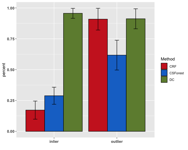
Figure 5: Achieved Type II errors for inliers (digits 0-5) outliers (digits 6-9) across 100 repetitions at $\alpha=0.05$ with merely 5 samples per-class in the test cohort.

Appendix A Proof of Theorem 3.2

Proof.

Here, we prove equation (3) for any given class $k$ and the test sample $x_{i}$, conditional on

1. Training samples other than $k$ and the bootstrap assignments $\mathcal{I}_{other}^{b}$ for $b=1,\ldots,\tilde{B}$.

2. Test samples other than $x_{i}$ and the bootstrap assignments $\mathcal{I}_{test}^{b}$ for $b=1,\ldots,\tilde{B}$.

For any training sample from class $k$, when comparing training sample $i^{\prime}$ to test sample $i$, we look at $\hat{f}^{i,i^{\prime}}(x;\mu)=\varphi(\{\hat{f}_{k}^{b}(x;\mu):i^{\prime}\notin I^{b}_{k},i\notin\mathcal{I}_{te}^{b}\})$ where $\varphi(.)$ is the mean-aggregation function. With some abuse of notations, we use $\{X_{i}\}_{i=1}^{n}$ to denote the set of training samples from class $k$ (e.g., $|\mathcal{I}_{k}|=n$), and $\mathcal{I}_{b}$ to denote a bootstrap of $\{X_{i^{\prime}}\}_{i^{\prime}=1}^{n}$ for $b=1,\ldots,B$ and $B\sim\rm{Binomial}(\tilde{B},(1-\frac{1}{n+1})^{n})$. Also, we use $\{(X_{n+1},Y_{n+1})\}$ to the test sample of interest (test sample $x_{i}$). For convenience, we also simply refer to $f^{ii^{\prime}}(x)$ as $\mu^{i^{\prime}}(x)$.

The above procedure can be equivalently characterized as sub-sampling $n$ samples with replacement from $\{X_{i^{\prime}}\}_{i^{\prime}=1}^{n+1}$ to form $\tilde{\mathcal{I}}_{b}$ for $b=1,\ldots,\tilde{B}$, and construct $\hat{\mu}^{i^{\prime}}(x)=\varphi(\{\hat{f}^{b}_{k}(x):X_{i},X_{n+1}\notin\tilde{\mathcal{I}}_{b}\})$. Under this alternative characterization, all $(n+1)$ samples receive invariant operations. We can similarly define the score function for each data pair $(X_{l},X_{j})$: $\mu^{l,j}(x)=\varphi(\{\hat{f}^{b}_{k}(x):X_{l},X_{j}\notin\tilde{I}_{b}\})$.

Define $A_{lj}=\mathbbm{1}\{\mu^{l,j}(X_{l})\geq\hat{\mu}^{j,l}(X_{j})\}$ for all $1\leq l,j\leq n+1$. It is obvious that $A_{ii}=1$ for all $i=1,\ldots,n+1$. Define $A_{l\bullet}=\sum_{j=1}^{n+1}A_{lj}$ as the sum of $l^{th}$ row from the comparison matrix A. By the construction of CSForest, we know that

$$k\notin\hat{C}_{l}(X_{n+1})\quad\mbox{if and only if}\qquad A_{n+1\bullet}\leq(n+1)\alpha-1.$$

Hence, (3) is equivalent to (A.1) below.

$$\mathbb{P}(A_{n+1\bullet}\leq(n+1)\alpha-1|Y_{n+1}=k)\leq 2\alpha.$$ (A.1)

We now proceed to prove (A.1), which consists of two steps (1) $A_{j\bullet}$ are exchangeable with each other for $j=1,\ldots,n+1$ when $Y_{n+1}=k$, and (2) the strange set $S(A)=\{j:A_{j\bullet}\leq(n+1)\alpha-1\}$ satisfies $|S(A)|\leq 2\alpha(n+1)$. Combining these two steps, we immediately have

$$\mathbb{P}\left[A_{n+1\bullet}\leq(n+1)\alpha-1|Y_{n+1}=k\right]$$

$$= \mathbb{P}\left[(n+1)\in S(A)|Y_{n+1}=k\right]=\frac{|S(A)|}{n+1}\leq 2\alpha.$$

At this stage, proofs to above two steps (1) and (2) become identical to that used in the proofs to Theorem 1 in Barber et al. (2021) or Theorem 1 in Kim et al. (2020).

∎

Appendix B More details on ACRF and ACRFshift

B.1 ACRF and ACRFrandom

ACRFrandom

In the original proposal of Romano et al. (2020), the authors assume that training and test data to have the same distribution. ACRFrandom defines a function $\mathcal{S}$ with input $x$, $u\in[0,1]$, the conditional probability $\pi_{y}=P(Y=y|X=x)$, and the threshold $\tau$. Define

$$\mathcal{S}(x,u;\pi,\tau)=\left\{\begin{array}[]{ccccccc}y\;indices\;of\;the\;L(x;\pi,\tau)-1\;largest\;\pi_{y}(x),&u<V(x;\pi,\tau)&\\ y\;indices\;of\;the\;L(x;\pi,\tau)\;largest\;\pi_{y}(x),&otherwise\end{array}\right.$$ (B.1)

where

$$V(x;\pi,\tau)=\frac{\sum_{c=1}^{L(x;\pi,\tau)}\pi_{(c)}(x)-\tau}{\pi_{(L(x;\pi,\tau))}(x)}$$ (B.2)

$$L(x;\pi,\tau)=\min\{c\in\{1,\cdots,C\}:\pi_{(1)}(x)+\pi_{(2)}(x)+\cdots+\pi_{(c)}(x)\geq\tau\}.$$ (B.3)

and $\pi_{(i)}(x)$ is the $ith$ largest conditional probability.

Further, ACRFrandom defines the generalized inverse quantile conformity score function $E$,

$$E(x,y,u;\hat{\pi})=\min\{\tau\in[0,1]:y\in\mathcal{S}(x,u;\hat{\pi},\tau)\}.$$ (B.4)

And the empirical distribution is

$$V(x,y;E)=\frac{1}{|\mathcal{I}_{cal}|+1}\sum_{i\in\mathcal{I}_{cal}}\delta_{E_{i}}+\frac{1}{|\mathcal{I}_{cal}|+1}\delta_{\infty}$$ (B.5)

where $E_{i}$ is constructed at the minimum $\tau$ for the calibration sample $i$ such that $y_{i}$ is included in $S(x_{i},u_{i};\hat{\pi},\tau)$ and $\delta_{i}$ denotes a point mass at $i$. The final prediction set is constructed as $\hat{C}(x)=\mathcal{S}(x,u;\pi,\hat{\tau}_{\alpha})$, where $\hat{\tau}_{\alpha}$ is the upper level $\alpha$ quantile of the empirical distribution $\{E_{i}\}_{i\in\mathcal{I}_{cal}}\cup\{\infty\}$.

ACRF

We can also consider a non-randomized version ACRF without the uniform variable $U$. For ACRF, we define

$$\mathcal{S}(x;\pi,\tau)=\{y\;indices\;of\;the\;L(x;\pi,\tau)\;largest\;\pi_{y}(x)\},$$ (B.6)

where

$$L(x;\pi,\tau)=\min\{c\in\{1,\cdots,C\}:\pi_{(1)}(x)+\pi_{(2)}(x)+\cdots+\pi_{(c)}(x)>\tau\}.$$ (B.7)

We can similarly define a score function $E$,

$$E(x,y;\hat{\pi})=\min\{\tau\in[0,1]:y\in\mathcal{S}(x;\hat{\pi},\tau)\},$$ (B.8)

and construct $E_{i}$ as the the minimum $\tau$ for the calibration sample $i$ such that $y_{i}$ is included in $S(x_{i};\hat{\pi},\tau)$. Same as in ACRFrandom, ACRF constructs as $\hat{C}(x)=\mathcal{S}(x;\pi,\hat{\tau}_{\alpha})$, where $\hat{\tau}_{\alpha}$ is the upper level $\alpha$ quantile of the empirical distribution $\{E_{i}\}_{i\in\mathcal{I}_{cal}}\cup\{\infty\}$. Algorithm 2 shows the details of ACRF.

1

Input : Training Data $\{z_{i}\coloneqq(x_{i},y_{i})^{n}_{i=1},i\in\mathcal{I}_{tr}\}$, Test Data $\{(x_{i})^{m}_{i=1},i\in\mathcal{I}_{te}\}$.

Output : Prediction sets $\hat{C}_{i}(x_{i})$ for $i\in\mathcal{I}_{te}$.

1 Randomly split the training data into 2 subsets, the training set $\mathcal{I}^{1}_{tr}$, the calibration training set $\mathcal{I}^{2}_{tr}$.

2Train random forest model $\mathcal{B}$ on all samples in $\mathcal{I}^{1}_{tr}$: $\hat{\pi}_{1}\leftarrow\mathcal{B}({(X_{i},Y_{i})}_{i\in\mathcal{I}^{1}_{tr}})$.

3Predict on $\mathcal{I}_{tr}^{2}$: $\hat{\pi}_{2}\leftarrow\mathcal{B}({(X_{i})}_{i\in\mathcal{I}_{2}})$ and $\mathcal{I}_{te}$: $\hat{\pi}_{te}\leftarrow\mathcal{B}({(X_{i})}_{i\in\mathcal{I}_{te}})$.

4Construct $\{E_{i}\}_{i\in\mathcal{I}^{2}_{tr}}$ treating $\mathcal{I}^{2}_{tr}$ as the calibration set.

5Compute the level $(1-\alpha)$ quantile of the empirical distribution $\{E_{i}\}_{i\in\mathcal{I}^{2}_{tr}}\cup\{\infty\}$.

6Use the function $\mathcal{S}$ defined in equation B.6 to construct the prediction set at $x_{i}\in\mathcal{I}_{te}$ as $\hat{C}_{i}(x_{i})=\mathcal{S}(X_{i};\hat{\pi}^{i}_{te},\hat{\tau}_{\alpha})$.

Algorithm 2 Implementation of ACRF

In Appendix B.3 shows the diffenrence between the randomized version and non-randomized version. To achieve a desirable type II error, we do not introduce the random variable $U$ in both ACRF and ACRFshift in the section 4.

B.2 ACRFshift

Under the covariate shift model, we can combine the proposal in Romano et al. (2020) with the covariate shift conformal prediction framework to perform better calibration (Tibshirani et al., 2019). This has not been discussed previously, so we give details about how this is done in our paper. We split also the test samples into two sets $\mathcal{I}_{te}^{1}$, $\mathcal{I}_{te}^{2}$. Suppose that we now construct the prediction set for test samples in $\mathcal{I}_{te}^{2}$.

Instead of finding $\tau$ with equation B.8 and B.5, we consider the following weighted calibration. The weighted function is $\gamma_{x}(x)=\frac{r(x)}{r(x)+\sum_{z_{i}\in\mathcal{I}_{2}}r(x_{i})}$ and $r(x)=\frac{\mathbb{P}[W=1|x]}{\mathbb{P}[W=0|x]}$ is the conditional probability of being generated from the test data ($W=1$ means from the test data, and $W=0$ represent from the training data), learned from the classifier separating the test data $\mathcal{I}_{te}^{1}$ from the training data $\mathcal{I}^{1}_{tr}$. Instead of consider $\hat{\tau}_{\alpha}$ as the level $(1-\alpha)$ quantile of the empirical distribution $\{E_{i}\}_{i\in\mathcal{I}^{2}_{tr}}\cup\{\infty\}$, for any $x\in\mathcal{I}_{te}^{2}$, we consider the level $(1-\alpha)$ quantile of the weighted distribution below:

$$V_{w}(x,y;E)=\sum_{i\in\mathcal{I}_{tr}^{2}}\gamma_{x}(x_{i})\delta_{E_{i}}+\gamma_{x}(x)\delta_{\infty}.$$

This can be applied also to both ACRF and ACRFrandom, resulting in ACRFshift and ACRFrandamShift respectively.

B.3 Randomized ACRF vs. Non-randomized ACRF

Table B.1 shows the type I error and type II error of ACRF/ACRFrandom and ACRFshift/ACRFrandomShift (referred to as non-randomized and randomized versions of ACRF/ACRFshift in Table B.1). We observe that models with randomness and those without randomness achieve comparable type I errors, while models with randomness tend to have worse type II errors and the final prediction set $\hat{C}$ is more likely to contain multiple labels. The possible reason is the purpose of randomized version to achieve the ideal conditional coverage may lead to redundant prediction sets and high type II error.

Table B.1: Randomized version vs. Non-randomized version: Achieved Type I and Type II errors at $\alpha=0.05$ with outlier components and no additional label shift among inlier digits and achieved Type I and Type II errors at $\alpha=0.05$ with label shift among inlier digits but no outlier digits.

Version	Method	no additional label shift		additional label shift
		Type I	Type II	Type I	Type II
Randomized	ACRF	0.049$\pm$0.007	0.702$\pm$0.017	0.025$\pm$0.007	0.884$\pm$0.014
	ACRFshift	0.053$\pm$0.007	0.681$\pm$0.014	0.055$\pm$0.013	0.828$\pm$0.015
Non-randomized	ACRF	0.047$\pm$0.006	0.431$\pm$0.003	0.171$\pm$0.024	0.313$\pm$0.067
	ACRFshift	0.036$\pm$0.009	0.439$\pm$0.009	0.080$\pm$0.026	0.630$\pm$0.127

B.4 Prediction bar-plots under traditional label-shift setting

FIGB.1 shows the per-class classification accuracy in the experiment of section 4.3. We observe that ACRF suffers from unbalanced classification performance for different digits where it has severe under-coverage for digits 3-5, resulting in its failure for marginal coverage under distributional changes in the test cohort. ACRFshift alleviates this phenomenon by taking into account the changes in the marginal density of $x$. However, it does not solve this issue completely and leads to a significant decrease in specificity compared to ACRF and CRF.

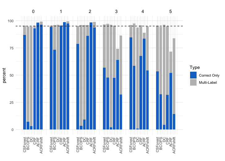
Figure B.1: Per-class quality evaluation of all methods under standard label shift setting. There is no group R (outlier digits) in this setting.

Appendix C Example 1 with varying $\gamma$ and sample sizes

In this section, we compare CSForest using default $\gamma=1$ (referred to as CSForest) with that from using two smaller $\gamma$ values $\gamma=0$ (referred to as CSForest0) and $\gamma=(1/\log n_{te})$ (referred to as CSForestLOG). We see that all three choices outperformed BCOPS under various sample size settings as we vary the per-class training sample size from 10 to 200 and per-class test sample size from 10 to 200. It is not also not supervising that CSForest achieved lower type II errors for inliers compared to CSForest0 and CSForestLOG. Interestingly, even for outlier detection, CSForest achieved top performance and is only slightly worse than CSForest0 and CSForestLOG when the size of outliers is small and much smaller than the inlier classes.

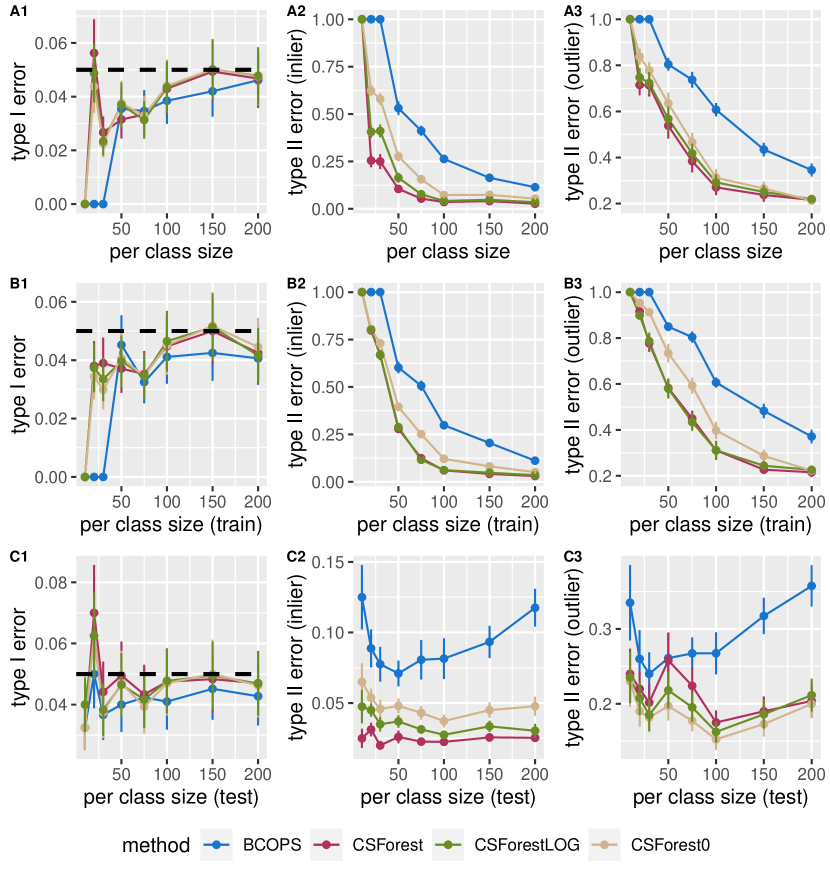
Figure C.1: FIGC.1A1-A3 show achieved type I error, type II error for inliers (class 1 and class 2), and type II error for outliers (class R) as we vary both per-class training sample size and per-class test sample size from 10 to 200. FIGC.1B1-B3 show these results as we vary per-class training sample size from 10 to 200 and keep the per-class test sample size at 200. FIGC.1C1-C3 show these results as we vary per-class test sample size from 10 to 200 and keep the per-class training sample size at 200.

References

- Barber et al. (2021) Barber, R. F., Candes, E. J., Ramdas, A., and Tibshirani, R. J. Predictive inference with the jackknife+. The Annals of Statistics, 49(1):486–507, 2021.
- Bartlett & Wegkamp (2008) Bartlett, P. L. and Wegkamp, M. H. Classification with a reject option using a hinge loss. Journal of Machine Learning Research, 9(8), 2008.
- Bickel et al. (2009) Bickel, S., Brückner, M., and Scheffer, T. Discriminative learning under covariate shift. Journal of Machine Learning Research, 10(9), 2009.
- Breiman (2001) Breiman, L. Random forests. Machine learning, 45(1):5–32, 2001.
- Charoenphakdee et al. (2021) Charoenphakdee, N., Cui, Z., Zhang, Y., and Sugiyama, M. Classification with rejection based on cost-sensitive classification. In International Conference on Machine Learning, pp. 1507–1517. PMLR, 2021.
- Chow (1970) Chow, C. On optimum recognition error and reject tradeoff. IEEE Transactions on information theory, 16(1):41–46, 1970.
- Cortes et al. (2016) Cortes, C., DeSalvo, G., and Mohri, M. Boosting with abstention. Advances in Neural Information Processing Systems, 29, 2016.
- Csurka (2017) Csurka, G. Domain adaptation for visual applications: A comprehensive survey. arXiv preprint arXiv:1702.05374, 2017.
- Esteva et al. (2017) Esteva, A., Kuprel, B., Novoa, R. A., Ko, J., Swetter, S. M., Blau, H. M., and Thrun, S. Dermatologist-level classification of skin cancer with deep neural networks. nature, 542(7639):115–118, 2017.
- Gretton et al. (2009) Gretton, A., Smola, A., Huang, J., Schmittfull, M., Borgwardt, K., and Schölkopf, B. Covariate shift by kernel mean matching. Dataset shift in machine learning, 3(4):5, 2009.
- Guan & Tibshirani (2022) Guan, L. and Tibshirani, R. Prediction and outlier detection in classification problems. Journal of the Royal Statistical Society: Series B (Statistical Methodology), 84(2):524–546, 2022. doi: https://doi.org/10.1111/rssb.12443. URL https://rss.onlinelibrary.wiley.com/doi/abs/10.1111/rssb.12443.
- Hechtlinger et al. (2018) Hechtlinger, Y., Póczos, B., and Wasserman, L. Cautious deep learning. arXiv preprint arXiv:1805.09460, 2018.
- Herbei & Wegkamp (2006) Herbei, R. and Wegkamp, M. H. Classification with reject option. The Canadian Journal of Statistics/La Revue Canadienne de Statistique, pp. 709–721, 2006.
- Kalra & Paddock (2016) Kalra, N. and Paddock, S. M. Driving to safety: How many miles of driving would it take to demonstrate autonomous vehicle reliability? Transportation Research Part A: Policy and Practice, 94:182–193, 2016.
- Kim et al. (2020) Kim, B., Xu, C., and Barber, R. Predictive inference is free with the jackknife+-after-bootstrap. Advances in Neural Information Processing Systems, 33:4138–4149, 2020.
- Kompa et al. (2021) Kompa, B., Snoek, J., and Beam, A. L. Second opinion needed: communicating uncertainty in medical machine learning. NPJ Digital Medicine, 4(1):1–6, 2021.
- Lei (2014) Lei, J. Classification with confidence. Biometrika, 101(4):755–769, 2014.
- Lin et al. (2005) Lin, J., Keogh, E., Fu, A., and Van Herle, H. Approximations to magic: Finding unusual medical time series. In 18th IEEE Symposium on Computer-Based Medical Systems (CBMS’05), pp. 329–334. IEEE, 2005.
- Lipton et al. (2018) Lipton, Z., Wang, Y.-X., and Smola, A. Detecting and correcting for label shift with black box predictors. In International conference on machine learning, pp. 3122–3130. PMLR, 2018.
- Marchette & Marchette (2001) Marchette, D. J. and Marchette, D. Computer intrusion detection and network monitoring: a statistical viewpoint. Springer, 2001.
- Ni et al. (2019) Ni, C., Charoenphakdee, N., Honda, J., and Sugiyama, M. On the calibration of multiclass classification with rejection. Advances in Neural Information Processing Systems, 32, 2019.
- Qayyum et al. (2020) Qayyum, A., Usama, M., Qadir, J., and Al-Fuqaha, A. Securing connected & autonomous vehicles: Challenges posed by adversarial machine learning and the way forward. IEEE Communications Surveys & Tutorials, 22(2):998–1026, 2020.
- Romano et al. (2020) Romano, Y., Sesia, M., and Candes, E. Classification with valid and adaptive coverage. Advances in Neural Information Processing Systems, 33:3581–3591, 2020.
- Schölkopf et al. (2012) Schölkopf, B., Janzing, D., Peters, J., Sgouritsa, E., Zhang, K., and Mooij, J. On causal and anticausal learning. arXiv preprint arXiv:1206.6471, 2012.
- Shimodaira (2000) Shimodaira, H. Improving predictive inference under covariate shift by weighting the log-likelihood function. Journal of statistical planning and inference, 90(2):227–244, 2000.
- Storkey (2009) Storkey, A. When training and test sets are different: characterizing learning transfer. Dataset shift in machine learning, 30:3–28, 2009.
- Tibshirani et al. (2019) Tibshirani, R. J., Foygel Barber, R., Candes, E., and Ramdas, A. Conformal prediction under covariate shift. Advances in neural information processing systems, 32, 2019.
- Vovk et al. (2005) Vovk, V., Gammerman, A., and Shafer, G. Algorithmic learning in a random world. Springer Science & Business Media, 2005.
- Vovk et al. (2018) Vovk, V., Nouretdinov, I., Manokhin, V., and Gammerman, A. Cross-conformal predictive distributions. In Conformal and Probabilistic Prediction and Applications, pp. 37–51. PMLR, 2018.