Revisiting Image Deblurring with an Efficient ConvNet
- Supplementary Material

In this supplementary material, we provide more details on the following topics: (1) all datasets that we employed in the network training (Sec.0.1), (2) the dilated structure that we consider in the ablation study (Sec.0.2), (3) the quantitative comparison on the LFDOF dataset [ruan2021aifnet] (Sec. 0.3), (4) the effective receptive field (ERF) and its evolution during the training (Sec. 1), and (5) additional qualitative comparisons of motion deblurring evaluated on the GoPro [nah2017deep], HIDE [shen2019human], and RealBlur [rim2020real] datasets, as well as defocus deblurring evaluated on the DPDD [abuolaim2020defocus], RealDOF [lee2021iterative], and CUHK [shi2014discriminative] datasets (Sec. 2).

We will make our code and weights publicly available.

0.1 Training

Here we provide more details on all the training and evaluation datasets for image motion and defocus deblurring tasks we use in this work.

Defocus deblurring We consider four defocus-related datasets. The most popular one is DPDD [abuolaim2020defocus], which collects blurry-sharp pairs separately with different aperture sizes using a DSLR camera. It has 350 training samples, and 76 testing samples for single-image defocus deblurring, as well as the dual-pixel version for dual-pixel defocus deblurring. RealDOF captures the data pairs in a single shot with a dual-camera setup, offering 50 high-resolution test samples. CUHK is collected for blur detection and provides 706 evaluated low-resolution samples acquired from the Internet. Note that RealDOF and CUHK have only testing samples and, thereby, are good for evaluating the generalization ability. LFDOF is a synthetic defocus blur dataset (11261 training samples and 725 testing samples) generated using a set of light field images, which in our experiment is adopted for the two-stage training strategy as proposed in [ruan2022learning].

Motion deblurring We consider three benchmark datasets – GoPro [nah2017deep], HIDE [shen2019human], and RealBlur [rim2020real]. The GoPro dataset features a synthetic blur that integrates adjacent frames from high-framerate videos to produce motion blur and contains 2013 blurry-sharp training pairs and 1111 testing samples. The HIDE dataset is synthesized following a similar method as the GoPro dataset but emphasizes human-aware deblurring, including large amounts of walking pedestrians, resulting in 6397 training and 2025 testing pairs. Here we follow [wang2022uformer, zamir2022restormer, zamir2021multi] and train our network on the GoPro dataset alone and directly evaluate the HIDE test set for demonstrating the generalization ability. The RealBlur dataset captures real motion blur and sharp images with a dual DSLR camera (Sony A7RM3) setup, which can be obtained simultaneously with different shutter speeds. It offers two subsets sharing the same content, one is output as JPEG images through a camera ISP, and the other is generated as raw images with white balance, demosaicing, denoising, geometric alignment, ., resulting in 3758 training samples and 980 testing samples for each set dubbed Real-J and Real-R. In our experiment, we train our network on the GoPro dataset and directly test it on the RealBlur dataset. We also train it on each RealBlur set for extra 450k iterations from the pre-trained weight using GoPro dataset as suggested in [rim2020real] and evaluate their associated testing sets.

In Tab. S1 we summarize the training and testing datasets used in the main manuscript.

Table 1: Summary of training and testing datasets for motion and defocus deblurring tasks.

	Datasets	Training	Testing
Motion	GoPro [nah2017deep]	2103	1111
	HIDE [shen2019human]	0	2025
	RealBlur-J[rim2020real]	3758	980
	RealBlur-R[rim2020real]	3758	980
Defocus	DPDD [abuolaim2020defocus]	350	76
	RealDOF [lee2021iterative]	0	50
	LFDOF [ruan2021aifnet]	11261	725
	CUHK [shi2014discriminative]	0	704
	Tab. / Fig.	Training	Testing
Motion	Tab. 1, Tab. 2 (upper), Fig. 6,	[nah2017deep]	[nah2017deep] & [shen2019human] & [rim2020real]
	Tab. 7, 9, 10	[nah2017deep]	[nah2017deep]
	Tab. 2 (lower), Fig. S9, S10	[rim2020real]	[rim2020real]
	Fig. S7, S8	[nah2017deep]	[nah2017deep] [shen2019human]
Defocus	Tab. 3, 4, 6 – 10, S0.2, Fig. 5, S11, S12	[abuolaim2020defocus]	[abuolaim2020defocus] & [lee2021iterative]
	Tab. 5, Fig. 7, S13, S14,S15, S16	[abuolaim2020defocus] & [ruan2021aifnet]	[abuolaim2020defocus], [lee2021iterative],[shi2014discriminative]
	Tab. S3	[ruan2021aifnet]	[ruan2021aifnet]

0.2 Ablation of network structure

Here we ablate our network with respect to its structure and layer number.

Version with dilated convolution layers As opposed to the LaKD block described in the main paper, here, we present its alternative version with dilated convolution layers (Fig. S1). Note that both versions aim to expand the effective receptive field. The dilated version adopts the same structure except for the feature mixing module that consists of three dilated convolution layers with increasing dilation rates. The results in Tab. 7 (refer to the main manuscript) further indicate the superiority of LaKD block.

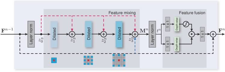
Figure 1: The structure of dilated convolution layers that can be compared with the corresponding structure in the LaKD block (refer to Fig. 2 in the main manuscript).

Layer number We ablate the layer number required in the feature mixing module, specifically on depthwise and pointwise convolution. For example, the label “one” in Tab. S0.2 denotes that the feature mixing module has one depthwise and one pointwise convolution layer. Table S0.2 shows that feature mixing equipped with two sequential depthwise and pointwise layers can reach the best performance.

Table 2: Layer number ablation in the feature mixing module.

2*[-0.45em] Number	DPDD			2*[-0.0em]Params.
(M)	2*[-0.0em]MACs
(G)
(rl)2-4	PSNR$\uparrow$	SSIM$\uparrow$	LPIPS$\downarrow$
one	26.10	0.808	0.155	15.4	1004
two (ours)	26.15	0.810	0.155	17.7	1208
three	26.09	0.806	0.156	20.1	1413

0.3 Performance on the LFDOF dataset

Following [ruan2022learning], we additionally investigate our network performance on the LFDOF dataset. AIFNet [ruan2021aifnet] has two subnets, sharing a similar spirit to the conventional methods that explicitly estimate the defocus map and then perform non-blind deconvolution. DRBNet [ruan2022learning] adopts an end-to-end solution and resorts to per-pixel kernel estimation to account for the spatially-varying blur. Our method is also an end-to-end solution that employs the LaKD block with a large effective receptive field, which leads to much better performance, as shown in Tab. S3.

Table 3: Quantitative comparison between AIFNet [ruan2021aifnet], DRBNet [ruan2022learning], and our network evaluated on 725 images from the LFDOF test set.

2*[-0.45em] Method	LFDOF
(rl)2-4	PSNR$\uparrow$	SSIM$\uparrow$	LPIPS$\downarrow$
AIFNet [ruan2021aifnet]	29.69	0.880	0.151
DRBNet [ruan2022learning]	30.40	0.891	0.145
Ours	31.87	0.912	0.115

1 ERF fitting details

In this section, we provide more details of our ERF visualization, GND-PDF fitting, and ERFMeter. We visualize all the ERFs and GND-PDF fittings of defocus deblurring networks [abuolaim2020defocus, son2021single, abuolaim2022improving, ruan2022learning, zamir2022restormer] in Fig. S2, variants of our networks that used for ablation study in Fig. S3, and our network with different kernel sizes in Fig. S4, correspondingly, all the parameters of GND-PDF fitting could be find in Tab. S4, Tab. S5, and Tab. S6. Besides, we also select several representative networks for motion deblurring [kupyn2018deblurgan, gao2019dynamic, cho2021rethinking, zamir2022restormer] and visualize their ERFs in Fig. S5. Note that the network structures are highly diverse, especially for networks on motion deblurring multi-patch [zhang2019deep], multi-scale [nah2017deep], recurrent scheme [park2020multi]. In this paper, we intend to reduce the diversity and only select networks with overall U-Net architecture so that the visualized ERFs are comparable.

We investigate the ERF [luo2016understanding] on the feature extracted from their bottleneck layer (the layer right before the first up-sampling in the decoder), which could potentially reveal the largest ERF they can achieve. The layer names corresponding to the bottleneck layer in each method are list in Tab. S4 to Tab. S7. The ERFs of networks for defocus deblurring are averaged from 912 image patches in size $512\times 512$, which are augmented from 76 testing images in DPDD dataset [abuolaim2020defocus] to further eliminate the dependence on input content, while ERFs of networks for motion deblurring are averaged from 1111 image patches in size $512\times 512$ from GoPro dataset [nah2017deep]. When doing GND-PDF curve fitting, the x-axis is empirically scaled from $[1,512]$ to $[-30,30]$ for higher fitting accuracy. We show the goodness of fitting $R^{2}$ for each network in Tab. S4 to Tab. S7.

ERF evolution during training We additionally demonstrate the ERF evolution during training for the motion and defocus deblurring tasks, as shown in Fig. S6. The ERF expands progressively with the training iterations and becomes much larger than at the initial stages. This observation is aligned with [luo2016understanding].

2 Additional qualitative results

In this section we show more qualitative results on motion and defocus deblurring. Note that we mainly compare our method with Restormer [zamir2022restormer] as it achieves state-of-art performance.

Motion deblurring We include additional visual results that are obtained using image samples from the GoPro (Fig. S7), HIDE (Fig. S8), Real-J (Fig. S9), and Real-R (Fig. S10) datasets. Those results complement Tabs. 1 and 2 in the main manuscript. Defocus deblurring We include visual results for single-image defocus deblurring for image samples from the DPDD (Fig. S11) and RealDOF (Fig. S12) datasets. Those results complement Tab. 3. We also provide visual results for dual-pixel defocus deblurring for image samples from the DPDD (Fig. S17) dataset, which complement Tab. 4. We further compare our method with DRBNet [ruan2022learning] adopting the two-stage training strategy proposed in [ruan2022learning], and we evaluate both methods using image samples from the DPDD (Fig. S13), RealDOF (Fig. S14), and CUHK (Fig. S15, S16) datasets, which complement Tab. 5.

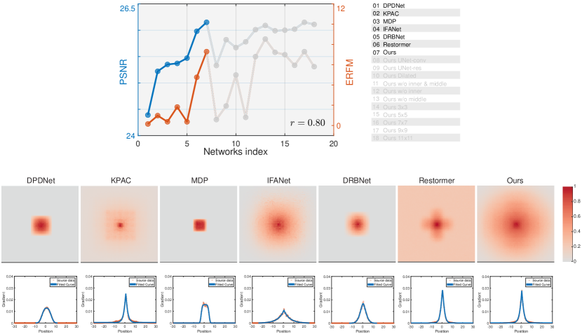
Figure 2: Demonstration of ERF patterns and the fitted GND-PDF curves: Here, different defocus deblurring networks are considered. Note that, the ERF patterns are in log scale for better visualization, while the GND-PDF curves are in linear scale.

Table 4: ERF fitting parameters and statistics for defocus deblurring networks.

Method	Layer Name	$\sigma$	$\beta$	$\mu$	$c_{1}$	$c_{2}$ (e-5)	$R^{2}$	PSNR	ERFM
DPDNet [abuolaim2020defocus]	conv5_2	5.2054	2.6054	0.9550	0.1188	-2.61	0.9978	24.39	0.1469
KPAC [son2021single]	conv4_4	1.8945	1.0838	0.8993	0.0923	41.47	0.9774	25.22	0.9737
MDP [abuolaim2022improving]	conv15	4.0575	4.9008	0.9371	0.1174	-0.32	0.9956	25.35	0.3658
IFANet[lee2021iterative]	conv_res	5.6632	0.9690	0.4738	0.1291	-18.31	0.9885	25.37	1.8221
DRBNet [ruan2022learning]	conv4_4	3.8936	1.5960	0.4254	0.1183	-1.79	0.9942	25.47	0.3615
Restormer [zamir2022restormer]	latent	1.9964	1.2687	0.5252	0.1057	19.14	0.9953	25.98	4.7581
Ours	bt_neck	1.9138	1.0812	0.5105	0.1044	21.27	0.9914	26.15	7.2870

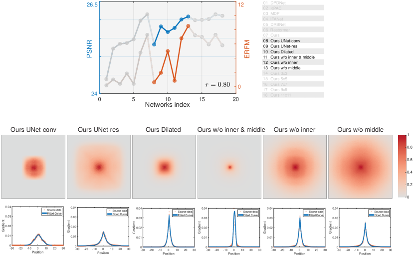
Figure 3: Demonstration of ERF patterns and the fitted GND-PDF curves: Here, different variants of our network are considered.

Table 5: ERF fitting parameters and statistics for variants of our network.

Method	Layer Name	$\sigma$	$\beta$	$\mu$	$c_{1}$	$c_{2}$ (e-5)	$R^{2}$	PSNR	ERFM
UNet-conv	bt_neck	6.2515	1.6787	0.7357	0.1224	-8.73	0.9841	25.33	0.5774
UNet-res	bt_neck	3.6274	1.0466	0.4065	0.1048	20.60	0.9873	25.82	1.9244
Ours-dilated	bt_neck	1.8397	1.1123	0.5869	0.1170	0.30	0.9812	25.67	4.9839
Ours w/o both	bt_neck	1.6120	2.1925	0.5965	0.1067	17.43	0.9047	25.78	0.7989
Ours w/o inner	bt_neck	1.8337	1.1069	0.5574	0.1089	13.79	0.9916	26.01	6.7925
Ours w/o middle	bt_neck	1.9742	0.9474	0.4418	0.1025	24.41	0.9845	26.09	8.5311

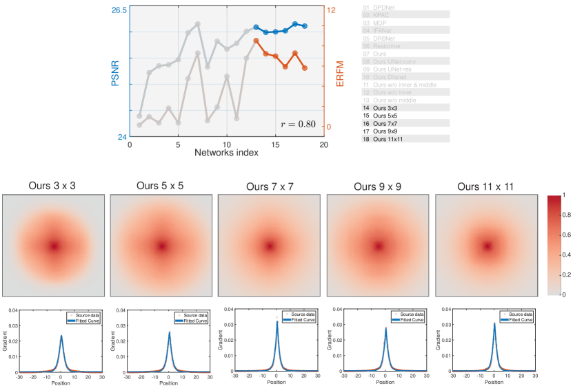
Figure 4: Demonstration of ERF patterns and the fitted GND-PDF curves: Here, we consider our network with different kernel sizes.

Table 6: ERF fitting parameters and statistics for our network with different kernel sizes.

Method	Layer Name	$\sigma$	$\beta$	$\mu$	$c_{1}$	$c_{2}$ (e-5)	$R^{2}$	PSNR	ERFM
ours ($3\times 3$)	bt_neck	2.3390	1.2508	0.4832	0.1032	23.31	0.9928	25.99	7.2201
ours ($5\times 5$)	bt_neck	2.0966	1.1722	0.5941	0.1024	24.59	0.9912	26.00	6.9847
ours ($7\times 7$)	bt_neck	1.6297	1.0267	0.5398	0.1071	16.86	0.9863	26.02	5.9340
ours ($9\times 9$)	bt_neck	1.9138	1.0812	0.5105	0.1044	21.27	0.9914	26.15	7.2870
ours ($11\times 11$)	bt_neck	1.7744	1.1446	0.4124	0.1067	17.42	0.9924	26.11	5.8027

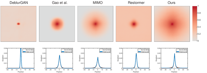
Figure 5: Demonstration of ERF patterns and the fitted GND-PDF curves: Here, different motion deblurring networks are considered.

Table 7: ERF fitting parameters and statistics for motion deblurring networks.

Method	Layer Name	$\sigma$	$\beta$	$\mu$	$c_{1}$	$c_{2}$ (e-5)	$R^{2}$	PSNR	ERFM
DeblurGAN [kupyn2018deblurgan]	ResnetBlock_18	1.1834	1.6237	0.0865	0.1145	4.44	0.9563	28.70	2.4235
Gao et al.[gao2019dynamic]	level3_deconv3_1	2.2912	1.2337	0.4046	0.1142	5.00	0.9967	30.90	5.3920
MIMO-UNet+ [cho2021rethinking]	DB3	2.4514	1.0489	0.2753	0.1077	15.78	0.9902	32.45	5.3514
Restormer [zamir2022restormer]	latent	1.9640	1.5154	0.5592	0.1054	19.63	0.9952	32.92	3.8813
Ours	bt_neck	1.7278	1.1311	0.5805	0.0977	32.52	0.9863	33.35	6.3704

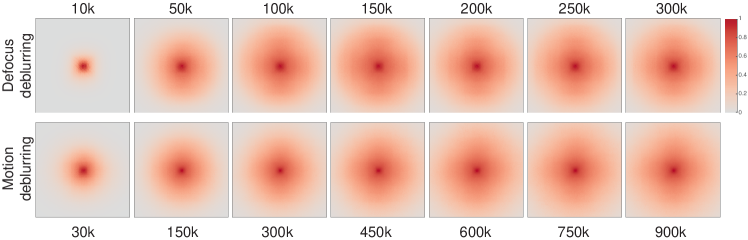
Figure 6: ERF evolution for increasing number of training cycles (from left to right) on defocus deblurring (up) and motion deblurring (down).

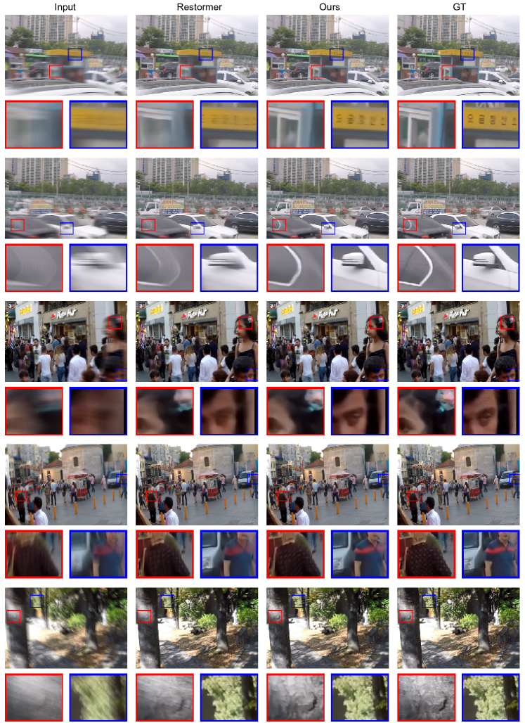
Figure 7: Qualitative comparison between Restormer [zamir2022restormer] and our method evaluated on GoPro dataset.

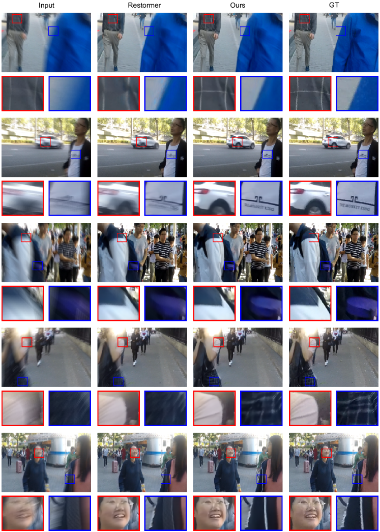
Figure 8: Qualitative comparison between Restormer [zamir2022restormer] and our method evaluated on HIDE dataset.

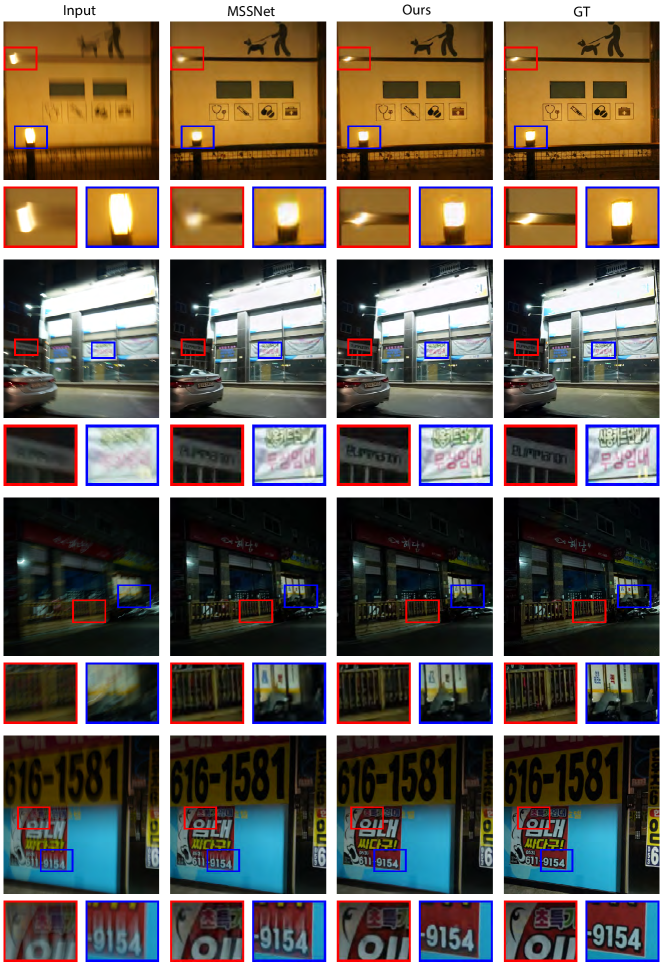
Figure 9: Qualitative comparison between MSSNet [kim2022mssnet] and our method evaluated on RealBlur-J dataset.

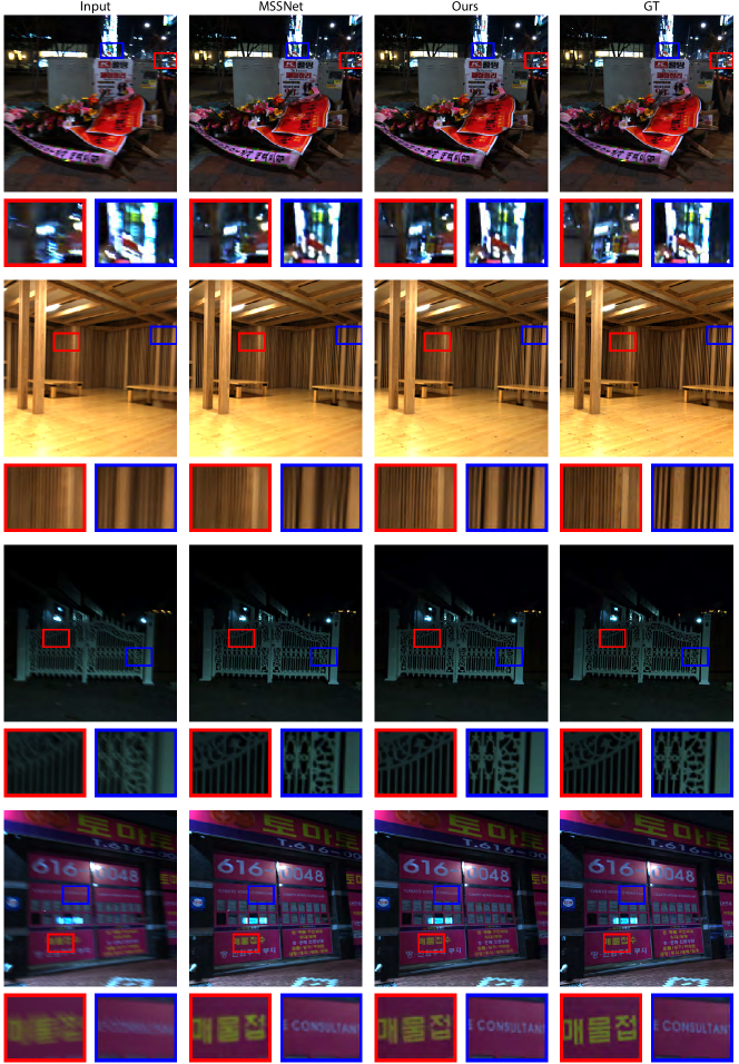
Figure 10: Qualitative comparison between MSSNet [kim2022mssnet] and our method evaluated on RealBlur-R dataset.

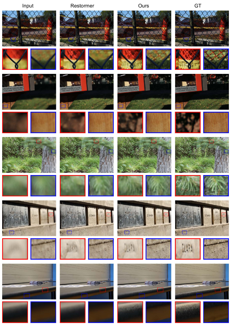
Figure 11: Qualitative comparison between Restormer [zamir2022restormer] and our method evaluated on DPDD dataset.

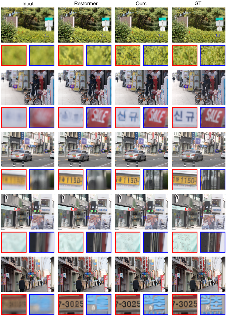
Figure 12: Qualitative comparison between Restormer [zamir2022restormer] and our method evaluated on RealDOF dataset.

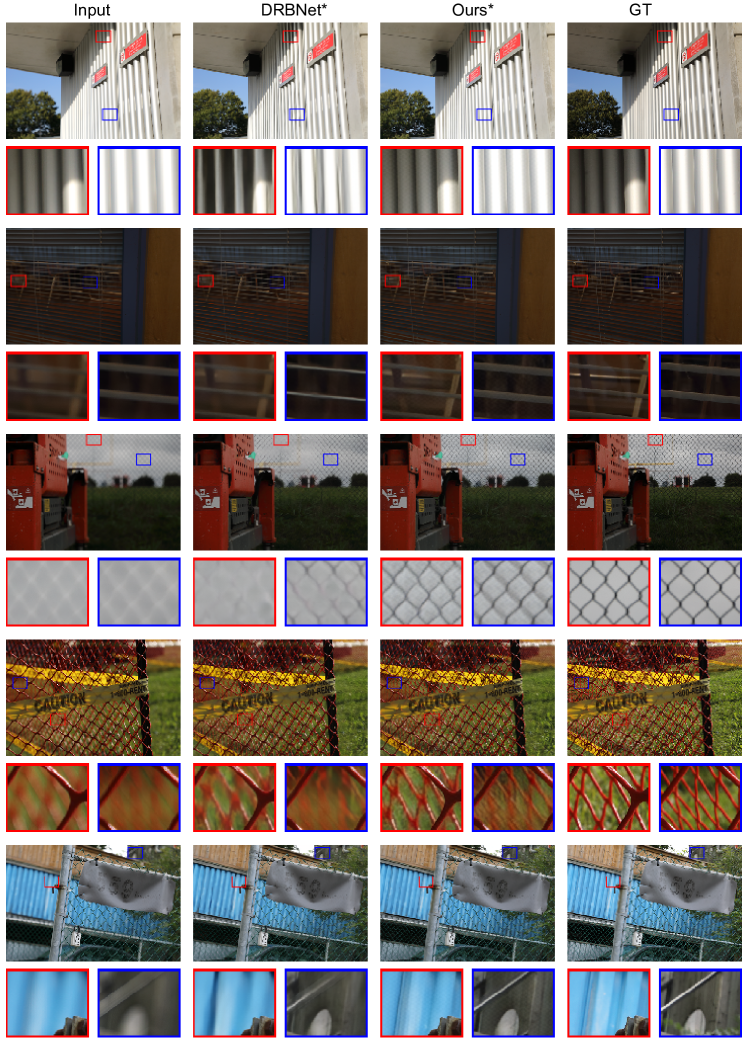
Figure 13: Qualitative comparison between DRBNet [ruan2022learning] and our method adopting the two-stage training strategy as proposed in [ruan2022learning] when evaluated on the DPDD dataset.

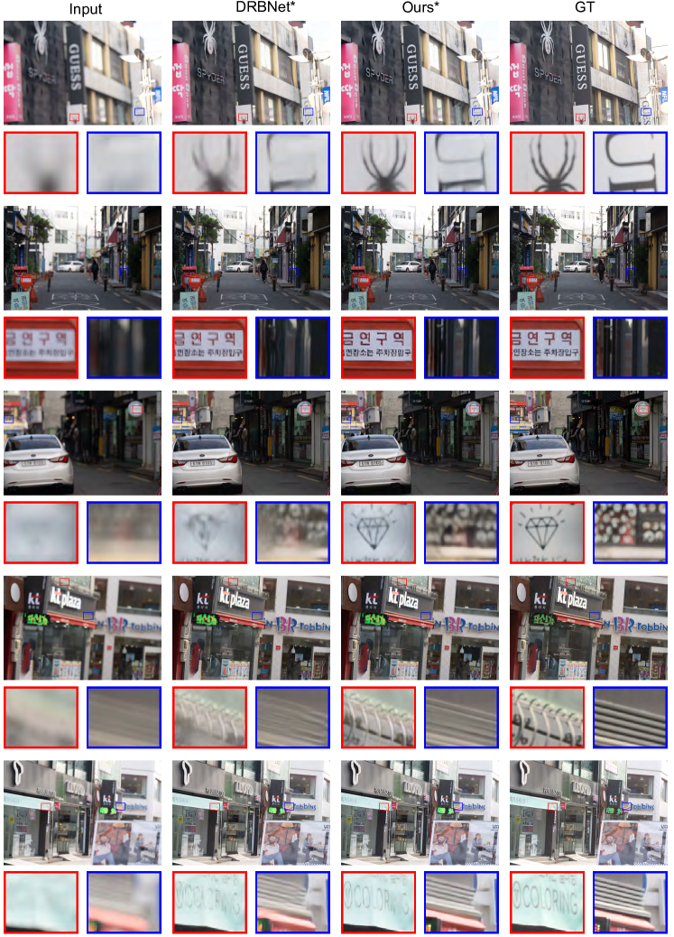
Figure 14: Qualitative comparison between DRBNet [ruan2022learning] and our method adopting the two-stage training strategy as proposed in [ruan2022learning] when evaluated on RealDOF dataset.

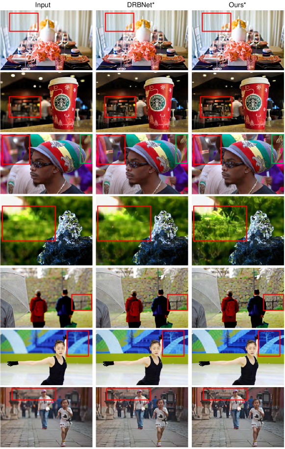
Figure 15: Qualitative comparison between DRBNet [ruan2022learning] and our method evaluated on CUHK dataset when adopting the training strategy proposed in [ruan2022learning]. Note no all-in-focus ground truth in CUHK dataset.

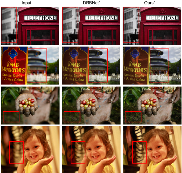
Figure 16: Qualitative comparison between DRBNet [ruan2022learning] and our method evaluated on CUHK dataset when adopting the training strategy proposed in [ruan2022learning]. Note no all-in-focus ground truth in the CUHK dataset.

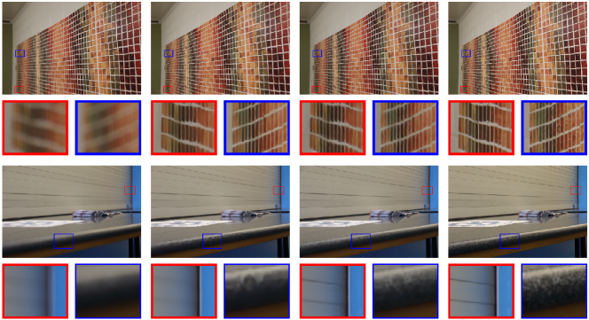
Figure 17: Dual-pixel defocus deblurring: Qualitative comparison between Restormer [zamir2022restormer] and our method evaluated on DPDD dataset.