Rank-based linkage I:
triplet comparisons and
oriented simplicial complexes
Abstract.
Rank-based linkage is a new tool for summarizing a collection of objects according to their relationships. These objects are not mapped to vectors, and “similarity” between objects need be neither numerical nor symmetrical. All an object needs to do is rank nearby objects by similarity to itself, using a Comparator which is transitive, but need not be consistent with any metric on the whole set. Call this a ranking system on . Rank-based linkage is applied to the -nearest neighbor digraph derived from a ranking system. Computations occur on a 2-dimensional abstract oriented simplicial complex whose faces are among the points, edges, and triangles of the line graph of the undirected -nearest neighbor graph on . In steps it builds an edge-weighted linkage graph where is called the in-sway between objects and . Take to be the links whose in-sway is at least , and partition into components of the graph , for varying . Rank-based linkage is a functor from a category of out-ordered digraphs to a category of partitioned sets, with the practical consequence that augmenting the set of objects in a rank-respectful way gives a fresh clustering which does not “rip apart“ the previous one. The same holds for single linkage clustering in the metric space context, but not for typical optimization-based methods. Open combinatorial problems are presented in the last section.
Keywords:
clustering, non-parametric statistics, functor, ordinal data, sheaf
MSC class: Primary: 62H30; Secondary: 05C20, 05E45,05C76
1. Introduction
1.1. Data science motivation
The rank-based linkage algorithm is motivated by needs of graph data science:
-
(a)
Summarization of property graphs, where nodes and edges have non-numerical attributes, but a node can compare two other nodes according to similarity to itself.
-
(b)
Graph databases require partitioning algorithms whose output remains stable when a batch of new nodes and edges is added.
-
(c)
Big data partitioning algorithms which are robust against data dropout, inhomogenous scaling, and effects of high degree vertices.
1.2. Topological data analysis paradigm
Topology is concerned with properties of a geometric object that are preserved under continuous deformations. Rank-based linkage is a new topological data analysis technique applicable, for example, to large edge-weighted directed graphs. Its results are invariant under monotone increasing transformations of weights on out-edges from each vertex. Equivalence classes of such graphs form a category under a suitable definition of morphism (Section 5.4) and rank-based linkage is a functor into the category of partitioned sets (of the vertex set) (Section 5.3.2), in a technical sense that satisfies (b) above. Single linkage clustering exhibits a similar functorial property in the case of finite metric spaces [12]; however, such functoriality is rare among unsupervised learning techniques.
1.3. Triplet comparison paradigm for data science
Consider exploratory data analysis on a set of objects, where relations are restricted to those of the form:
object is more similar to object than object is.
Kleindessner & Von Luxburg [29] call such a relation a triplet comparison. Readers may be familiar with triplet comparison systems arising from a metric on , where the relation means . In sequels to this paper, we will argue that a broader class of triplet comparison systems (mostly not arising from a symmetric dissimilarity measure) is natural in data science applications.
1.4. Presentations of ranking systems
There are several equivalent ways to present triplet comparison systems, each useful in its own context. These include:
-
(a)
Comparator places a total order on for each object , where whenever ; Comparator is an interface in the Java language [27].
-
(b)
For each , a bijection assigns ranks to objects other than . Collect these bijections into an ranking table , whose entry is the rank awarded to object by the ranking based at object , taking . The ranking table (e.g. Table 1) is an efficient data storage device.
- (c)
1.5. Orientations of the line graph
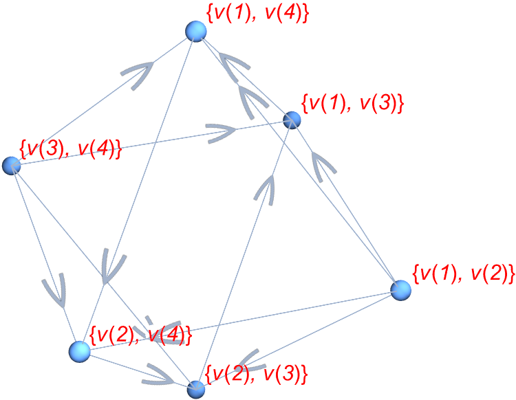
The reader is advised to study Figures 1 and 2 carefully. The former shows the complete graph , where the label on a directed edge means that is ranked by among the elements of . Figure 2 shows the corresponding line graph , whose vertices (“0-simplices”) are unordered pairs of objects, and whose edges (“1-simplices”) are pairs such as with an element in common. Interpret a triplet comparison as an assignment of a direction to a specific edge of the line graph: . From now on we will abbreviate this to . To emphasize: the ranks which appear as labels on directed edges of the complete graph (Figure 1) provide directions of the arcs of the line graph (Figure 2). The combinatorial input to data science algorithms will be a simplicial complex, consisting of a subset of the vertices, edges, and triangular faces (“2-simplices”) of the line graph , after orientations are applied to the 1-simplices. Full details are found in Section 3.
Our use of simplicial complexes is distinct conceptually from other uses in network science, such as [26]. Warning: the objects of are not the vertices of the simplicial complex.
1.6. Enforcer triangles and voter triangles
A careful look at Figure 2 shows that there are two kinds of triangular faces: the first kind, called enforcers, take the form
| (1) |
where the arrows declare that, under the comparator at , the integers in the rank table satisfy . Enforcer triangles are enforcing transitivity of the total order induced by ’s ranking. In an enforcer triangle, four distinct objects in are mentioned.
There remain the second kind of triangles, called voters, where for distinct ,
| (2) |
The arrows declare that the integers in the rank table satisfy , , and . A voter triangle mentions only three objects, each of which (here , , and ) “votes” on a preference between between the other two. See Figure 11 for more examples.
1.7. Three kinds of ranking system
-
(1)
A ranking system (without ties) corresponds to an arbitrary ranking table, and to an orientation of such that all the enforcer triangles are acyclic. There are no restrictions on the voter triangles.
- (2)
-
(3)
Intermediate between (1) and (2) are the 3-concordant ranking systems, in which there are no directed 3-cycles. In other words, both enforcer triangles and voter triangles are acyclic; however, cycles are allowed among loops of length four or greater. It appears that 3-concordant ranking systems are especially appropriate for rank-based algorithms based on triplet comparisons, and include ranking systems not arising from metrics on . Table 1 and Figure 12 show examples.
| object | 0 | 1 | 2 | 3 | 4 | 5 | 6 | 7 | 8 | 9 |
|---|---|---|---|---|---|---|---|---|---|---|
| 0 | 7 | 6 | 4 | 8 | 3 | 1 | 5 | 9 | 2 | |
| 5 | 0 | 3 | 6 | 7 | 8 | 1 | 4 | 9 | 2 | |
| 7 | 6 | 0 | 1 | 9 | 5 | 3 | 4 | 8 | 2 | |
| 2 | 9 | 5 | 0 | 4 | 6 | 3 | 8 | 7 | 1 | |
| 9 | 8 | 7 | 4 | 0 | 3 | 6 | 2 | 1 | 5 | |
| 4 | 9 | 3 | 6 | 5 | 0 | 1 | 7 | 8 | 2 | |
| 1 | 6 | 5 | 4 | 8 | 3 | 0 | 7 | 9 | 2 | |
| 7 | 9 | 1 | 8 | 2 | 3 | 5 | 0 | 4 | 6 | |
| 9 | 6 | 7 | 5 | 1 | 3 | 8 | 2 | 0 | 4 | |
| 7 | 5 | 4 | 2 | 8 | 3 | 1 | 6 | 9 | 0 |
1.8. Natural examples of non-metric ranking systems arise in data science
In Section 2.3 edge-weighted digraphs will be seen as the prototypical examples of non-metric ranking systems; see Section 2.12.2. Meanwhile, here are some examples of more specific comparators.
-
•
Lexicographic comparators in property graphs: Each object in has multiple categorical fields. For example a packet capture interface may specify fields such as source IP, destination IP, port, number of packets sent, and time stamp. List these in some order of importance. Given , decide whether or is more similar to by passing through the fields in turn, comparing the entries for and in that field with the entry for . The first time agrees with while differs, or vice versa, the tie is broken in favor of the one which agrees with . The Comparator.thenComparing() method in the Java language [27] implements this.
-
•
Information theory: consists of finite probability measures, and if Kullback-Leibler divergence , where This is generally not 3-concordant: see [8].
-
•
is the state space of a Markov chain with transition probability , and if . Random walk on a weighted (hyper)graph gives a concordant ranking system, as will be explained in a future work.
-
•
is a collection of senders of messages on a network during a specific time period. Declare that if sends more messages to than to , or if sends the same number to each but the last one to was later than the last one to . In contrast to undirected graph analysis, messages received by play no part in its Comparator.
Why do we favor 3-concordant ranking systems over concordant ones? For algorithms such as rank-based linkage (Algorithm 1) and partitioned local depth [9] which study triangles in which a particular 0-simplex (i.e. object pair) is a source, the extra generality is welcome, and carries no cost because cycles longer than three do not matter. On the other hand a 3-cycle appears as a “hole” in the data, and is something we prefer to avoid.
1.9. Goal and outline of present paper
The influential paper of Carlsson and Memoli [12] has illuminated the defects of many clustering schemes applied to finite metric spaces. In particular these authors postulate that a clustering algorithm should be a functor from a category of finite metric spaces to a category of partitioned sets (Section 5.2).
Section 5 supplies a categorical framework which offers a functorial perspective on clustering schemes for ranking systems. This perspective suggests a specific hierarchical clustering scheme called rank-based linkage. Our main result is Theorem 5.31, verifying that rank-based linkage is a functor between suitable categories.
As for the rest of the paper:
-
(a)
Users of our algorithm will find all the practical details they need in Section 2.
-
(b)
Section 3 on sheaves and simplicial complexes supplies the structural rationale for the design of the algorithm.
-
(c)
Section 4 proves combinatorial properties which establish algorithm correctness.
-
(d)
Section 5 derives functorial properties, with full category theory precision.
-
(e)
Section 6 describes how the algorithm behaves when two experimenters merge their data — an important but neglected aspect of data science.
- (f)
1.10. Related literature
Clustering based on triplet comparisons has been been studied by Perrot et al. [40], who attempt to fit a numerical “pairwise similarity matrix” based on triplet comparisons. Mandal et al. [35] consider hierarchical clustering and measure the goodness of dendrograms. Their goals are different to ours, which can be seen as a scalable redesign of [9].
2. Hierarchical clustering based on linkage
2.1. Need for -nearest-neighbor approximation
In this section we deal with practical graph computation on billion-scale edge sets. The number of voter triangles for a ranking system on objects is , which is impractical at this scale; indeed, cubic complexity limits the application of the related PaLD algorithm [9]. To dodge this burden, we work with a -nearest-neighbor approximation111 In suitable settings [8], this could be achieved with work by -nearest neighbor descent. to the ranking system. This lowers the computational effort from to , and memory from to . The integer should be large enough so that the nearest neighbors of any object provide sufficient data for clustering decisions, but small enough so that linking decisions are “local” (these are informal, not mathematical, definitions).
2.2. Out-ordered digraphs
Assume that a set of objects is given, on which a ranking system exists, expressed by a family of comparators. Suppose that a set of no more than nearest neighbors222 When is the vertex set of a sparse graph, is typically a subset of the graph neighbors of . If a vertex has degree less than , then . of object , has been computed, for each , such that all the elements of are ranked by as closer to than any elements of . Results later in the paper do not depend on whether the sets have identical cardinality, but the upper bound is used in complexity estimates. When , we shall say “ is a friend of ”. Call and “mutual friends” if and . There is no need for a full ranking of according to which would be work in total, but only a ranking of :
Definition 2.1.
Given a ranking system on a set , the out-ordered digraph on with respect to friend sets is the restriction of each comparator to the friends of , for all . Abbreviate this to .
2.3. Concrete presentation as edge-weighted digraph
Consider edge-weighted directed graphs on , whose arcs consist of:
The weight on the arc is denoted , and the weight function is denoted . Interpret as a scale-free measure of similarity of to , as perceived by . We further require that, for each , the values are distinct real numbers. Introduce an equivalence relation on such edge-weighted digraphs as follows.
Definition 2.2.
Edge-weighted digraphs and are rank-equivalent if , for all , and if for each , the total ordering of according to and the total ordering according to coincide.
We omit the proof of the following assertion.
Lemma 2.3.
An out-ordered digraph on is an equivalence class of rank-equivalent digraphs. Weighted digraph belongs to this equivalence class if for all ,
| (3) |
Definition 2.4.
Such a representative of the equivalence class of an out-ordered digraph on , satisfying (3), is called a representative out-ordered digraph.
Canonical example: Take if is ranked among the friends of .
Practical significance: Lemma 2.3 allows us to perform rank-based linkage computations using any directed edge-weighted graph in the correct equivalence class of out-ordered digraph on , provided the weights of arcs are used only for comparison, and not for arithmetic. Contrast this with graph partitioning based on the combinatorial Laplacian [36]: in the latter case, numerical values of edge weights form vectors used for eigenvector computations, which are sensitive to nonlinear monotonic transformations.
2.4. Undirected graph from an out-ordered digraph on
The algorithm also uses a “forgetful view” of the out-ordered digraph, depending only on the friend sets . By abuse of notation, we shall use the familiar term “-NN” although some friend sets may have fewer than elements.
Definition 2.5.
The undirected -neighbor (-NN) graph consists of all the arcs in the out-ordered digraph, stripped of their direction and weight.
Later Definition 5.2 revisits this notion in a more formal way.
Assume henceforward that every object has degree at least two in the graph . This condition is enforced [14] by restricting all subsequent computation to the (undirected) two-core of an input digraph, before taking the -neighbors of each vertex.
2.5. Rank-based linkage algorithm: overview
If we were dealing with a full ranking system on , not just comparators on friend sets, then the hierarchical clustering algorithm in this section can be over-simplified as
Link a pair of objects if the corresponding 0-simplex of the line graph is the source
in at least voter triangles, for suitable . Then partition according to graph components.
When we deal with an out-ordered digraph on (Definition 2.1), more subtlety is needed; we restrict the 0-simplices, and Definition 4.1 will determine which voter triangles qualify for inclusion.
2.6. Data input: edge-weighted digraph
In our Java implementation [14], the input to the rank-based linkage algorithm is a flat file, possibly with billions of lines, presenting a representative of an out-ordered digraph (Definition 2.4). Each line takes the form , regarded as a directed edge from object to object , with weight of some type which is Comparable333 The Java [27] interface Comparable is implemented by any type on which there is total ordering, such as integers and floating point numbers. .
Let us emphasize that only the relative values of are important. For example, can be taken as minus the rank of in the ordering of given by .
The cut-down to nearest neighbors may or may not have been done in advance. In either case, our Java implementation [14] reads the file and stores it in RAM in the data structure of a directed edge-weighted graph, with out-degree bounded above by .
2.7. Canonical rank-based linkage algorithm
Here are the steps of the rank-based linkage algorithm, based on the graphs of Definitions 2.4 and 2.5, which are concrete expressions of Definition 2.1. Its rationale emerges from the functorial viewpoint of Section 5.
The algorithm will create a new undirected edge-weighted graph called the linkage graph (Definition 4.6) whose links are the pairs of mutual friends, and whose weight function is called the in-sway. We shall describe this first in text, and then in pseudocode as Algorithm 1.
-
(a)
Determine the set of pairs of mutual friends: these are the links .
-
(b)
Iterate over the links , possibly in parallel.
-
(c)
For each pair of mutual friends, iterate over among the common neighbors of and of in the undirected graph . Count those for which three conditions hold:
-
•
is non-empty.
-
•
is distinct from and .
-
•
is the source in the voter triangle . The two ways can be the source444 All the 1-simplices have a well-defined direction, as we shall see in Definition 4.1. This triangle must have a source and a sink if the out-ordered digraph is 3-concordant. are:
(4) or
-
•
-
(d)
The count obtained in (c) is the in-sway .
-
(e)
At the conclusion of the iteration over , the linkage graph is finished. It supplies a monotone decreasing sequence of undirected subgraphs where is defined to be the set of links whose in-sway is at least .
- (f)
-
(g)
If , the critical in-sway is the largest value of for which . The sub-critical clustering consists of the graph components of ; it is recommended as a starting point for examining the collection of partitions.
2.8. Design and typical applications of the algorithm
2.8.1. Does the ranking system need to be 3-concordant?
The in-sway computation (4) requires a decision about the source of each voter triangle. If there were a 3-cycle in the line graph, the corresponding voter triangle would be “missing data”. Thus 3-concordance is preferred, but a few exceptions (such as may occur in the Kullback-Leibler divergence example of Section 1.8) merely induce some bias, and may be tolerated.
2.9. Does every object need to have exactly friends?
If the friends are a subset of the neighbors of in a sparse graph, then it will sometimes happen that . This makes such a “less influential” than an object with neighbors, in that it participates in fewer voter triangles; this does not upset the algorithm much. On the other hand if but we allow one specific with , then this will be “excessively influential”, in the sense that in (c) it will participate in many more voter triangles than a typical object does. This would introduce a more serious bias, which we prefer to avoid.
2.10. Typical input format
Our initial input takes a list of object pairs with weight as input: this is interpreted as edge data for an edge-weighted graph which may be either directed or undirected, according to a run time parameter.
2.11. Compute effort
2.12. Computational examples
2.12.1. Ten point set
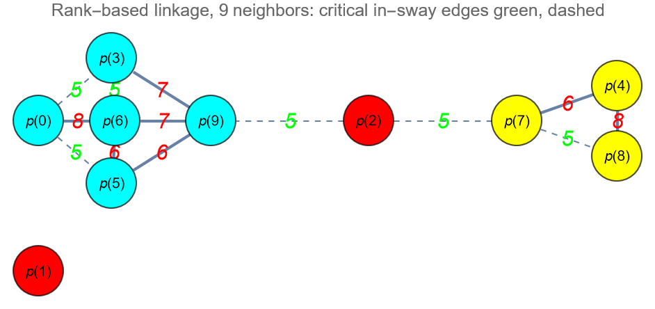
Figure 3 shows rank based linkage on the ten objects whose ranking system appears in Table 1, with for each . Observe that the pairs and both exhibit the maximum possible value of in-sway, which is 8. Verify in Table 1 that each of these 0-simplices is the source in all 8 of the voter triangles in which it occurs. The sub-critical clustering gives 4 clusters, namely two singletons, and clusters of sizes three and five, respectively.
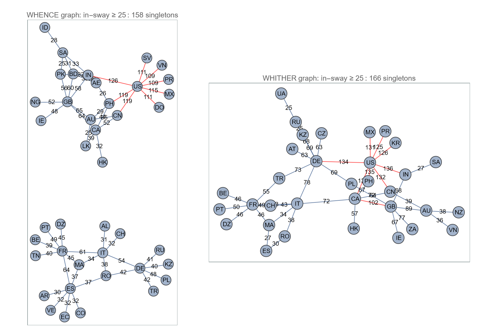
2.12.2. Digraph example: migration flows among 200 countries
Azose & Raftery [4] build a statistical model, based on OECD data, to estimate how many persons who lived in country in 2010 were living in country in 2015. They take account of both migration and reverse migration, as distinct from net migration often seen in official figures. Starting from their table of flows in [4], we selected flows of size at least 1000 persons, and built a sparse directed weighted graph with 3866 edges. Our Java code [14] found the 2-core (199 countries), then 8 nearest neighbors of each country under each of two comparators:
-
(a)
WHENCE comparator: if flows from country to country exceed flows from country to . Whence are immigrants coming from?
-
(b)
WHITHER comparator: if flows from country to country exceed flows from to country .Whither are our citizens emigrating?
Using each comparator, a portion of the linkage graph is shown in Figure 4. Country digraphs are listed at immigration-usa.com/country_digraphs.html.
Switching between a source-base comparator and a target-based comparator is an option for rank-based linkage on any weighted digraph.
2.12.3. Run times on larger graphs
Table 2 shows some run times for our initial un-optimized Java implementation [14], with JDK 19 on dual Xeon E3-2690 (48 logical cores).
| Digraph prep. | Rank-based linkage | Components | RAM | ||
|---|---|---|---|---|---|
| 1M. | 8 | 16 secs | 5 secs | 5 secs | 8 GB |
| 10M. | 8 | 228 secs | 44 secs | 49 secs | 78 GB |
3. Sheaves on a simplicial complex
3.1. Geometric intuition
Sheaves [13] on a simplicial complex supply a toolbox for precise description of rank-based linkage. Figures 1 and 2 supply geometric intuition. The six points, twelve edges, and eight triangles of the octahedron shown in Figure 2 are the 0-cells, 1-cells, and 2-cells, respectively of an abstract simplicial complex. The 3-concordant ranking system shown in Figure 1 leads to an orientation of the 1-cells such that none of the 2-cells is a directed 3-cycle. This orientation of the 1-cells provides a toy example of an oriented simplicial complex.
Including all the points, edges, and triangles of the line graph of the complete graph of leads to an excessive computational load for large . The next section outlines a parsimonious approach.
3.2. A 2-dimensional simplicial complex based on a line graph
Take a graph on the set , and then take a subgraph of the line graph , whose vertex set is all the edges of . We are going to build a two-dimensional abstract simplicial complex whose 0-cells, 1-cells, and 2-cells are the points, edges, and triangles, respectively, of . To be precise, is defined as follows:
-
0:
The 0-cells or 0-simplices of are the edges of . A typical element of will be abbreviated to , for distinct adjacent .
-
1:
The 1-cells or 1-simplices are the edges of , i.e. pairs for distinct 0-cells and 666 Note that and are non-adjacent in the line graph, for distinct . .
- 2:
When is the complete graph on , and is the line graph , we obtain the points, edges, and triangles, respectively, of this line graph. This complex imposes at least a cubic computational burden, because has elements.
Recall that an orientation of a graph means an assignment of a direction to each edge. An orientation of the simplicial complex means an orientation of .
We repeat, in simplicial complex notation, the definitions of Section 1.4.
Definition 3.1.
A ranking system on is an orientation of the -cells of (i.e. edges of the line graph) such that 2-cells of the form are acyclic, for distinct in . If 2-cells of the form are acyclic also, call the ranking system 3-concordant. Call it concordant if the orientation of the entire line graph is acyclic.
3.3. Oriented simplicial complex associated with out-ordered digraph
Given an out-ordered digraph (Definition 2.1), take the graph of Section 3.2 to be the undirected -NN graph (Definition 2.5), denoted . Choose a subgraph of the line graph of as follows: the vertex set of is , and the edges of consist of pairs such that . This last condition is crucial. The edge set is computable from the out-ordered digraph according to the rules laid out above.
We make this choice of so that its edges acquire an orientation from the out-ordered digraph. In the first place if and ; secondly if , the comparator at is able to compare and , because
| (5) |
with the arrow reversed if . Here the important notion is: a non-friend of is less similar to than is a friend of . The computational advantage of using versus the whole line graph is that has at most elements.
According to the pattern of Section 3.2, define an oriented simplicial complex
| (6) |
as follows:
-
0:
The 0-cells , i.e. edges of the undirected -NN graph.
-
1:
The 1-cells are pairs such that , with an orientation acquired from the out-ordered digraph .
-
2:
The 2-cells are triples of 0-cells, all of whose 1-faces are in (see Definition 4.1 for consequences). If the ranking system is 3-concordant, none of these 2-cells is cyclic according to the orientation of its 1-faces.
Rank-based linkage computations (Algorithm 1) make reference to this oriented simplicial complex, without explicitly constructing it.
Definition 3.2.
An out-ordered digraph is called 3-concordant (resp. concordant) if the induced orientation of is 3-concordant (resp. concordant).
3.4. Sheaf perspective
Let be any abstract simplicial complex (for example above, but the restriction to 0-cells, 1-cells, and 2-cells seems unnecessary). Associate with the poset of simplices, ordered by containment, and the topology whose basic open set consists of the collection of faces contained within any given simplex. For example, the 2-cell (abbreviated to ) is associated with a basic open set
in the notation where the 1-cell is abbreviated to . Contained within are the basic open sets , , and , but these do not cover .
If are distinct 0-simplices, say that -simplices form a -loop. For example, given any face , forms a -loop.
Definition 3.3.
Let be the presheaf such that is the set of orientations of the -simplices of that are -acyclic in the strong sense that does not contain vertices and edges , , oriented as indicated, even if the -simplex does not belong to . More generally, let be the set of orientations of the 1-simplices of such that all -loops of -simplices of are acyclic, for all . For we interpret this notation as the set of concordant orientations; for , as the set of all orientations.
is a separated presheaf with respect to the topology on , because the restriction map is the composite when and two sections that agree on an open cover are equal. Examples of this construction include:
-
(a)
If is the basic open set associated with a 2-cell, there are six elements in ; out of orientations of the three 1-simplices, all but two are acyclic.
-
(b)
If as in Definition 3.1, then (resp. ) coincides with the 3-concordant (resp. concordant) ranking systems on .
-
(c)
is formally a 1-element set for all .
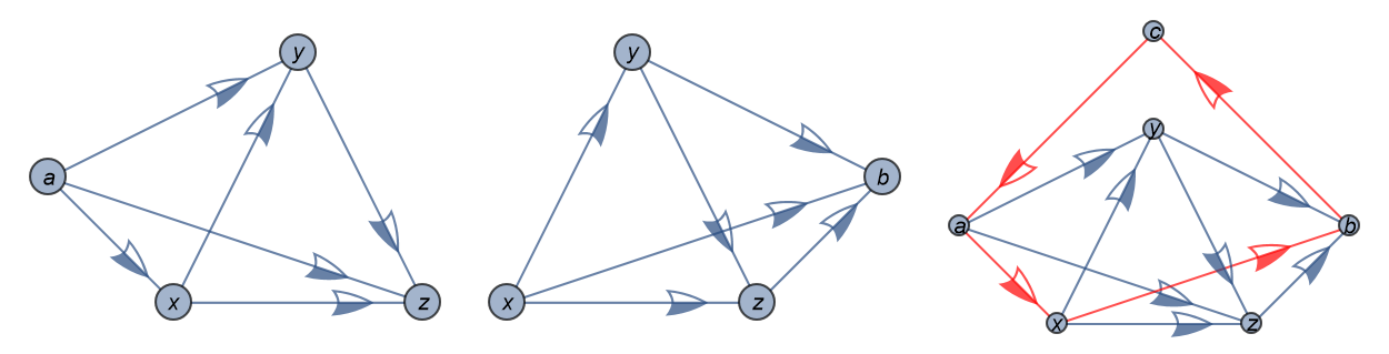
It is easy to see that is not a sheaf for , by considering a simplicial complex with vertices and edges for with indices read mod . If the edges are oriented by to form a -loop, then the obvious sections on the open sets containing and its endpoints do not glue to any section of . This is illustrated in Figure 5 for .
3.5. 3-concordant ranking systems form a sheaf
We now show how to modify the definition of so as to define a sheaf . Unfortunately it does not appear that there is any analogous modification of that would allow us to define a sheaf of -concordant orientations on a simplicial complex of dimension when .
Definition 3.4.
For any open set let be the set of orientations of the 1-simplices of that are acyclic on all 2-simplices of , i.e., with no 2-simplex whose 1-faces have orientations , , .
Definition 3.5.
More generally, for a positive integer let be the set of orientations of the -simplices of that are acyclic on all simplices of of dimension less than .
Note that if then . Also, for every orientation of the -simplices of belongs to .
Remark: The definition of is significant in framing the definition of the rank-based linkage clustering algorithm in Section 4. For one thing, it naturally separates the ranking systems from the -concordant ranking systems: ranking systems are sections of , where is the open subset that omits all voter triangles, i.e. -cells bounded by . In terms of the language in Definition 4.1, this allow us to prohibit certain triangles automatically from being -pertinent, which would correspond to using a smaller simplicial complex that omits certain 2-simplices.
Example 3.6.
Definition 3.4 does not impose any condition on these three edges if is not a -simplex of . For example, suppose that is the -skeleton of a -simplex . Then and agree, since they equal the -element set of acyclic orientations of the -faces of . However, and differ: , while is the -element set of all orientations of the -faces of .
Proposition 3.7.
(Definition 3.5) is the sheafification of . In particular it is a sheaf.
Proof.
Let be an open set. The sections of the sheafification of over are compatible collections of sections on open covers of mod the relation that identifies pairs of such collections that agree after further refinement. In particular, let be the maximal simplices contained in . Every open cover of must contain at least one open set that includes and therefore its edges; thus the orientation must have no cycles of length or less on the edges of . On the other hand, by considering an open cover with one set for each simplex in , we see that there are no further conditions.
Clearly a section of the sheafification over determines an orientation of the -simplices in uniquely (that is, equivalent collections of sections on open covers determine the same orientation), and conversely an orientation with no cycles of length or less on the determines a section over . We thus see that, for every , the sections of and of the sheafification of are in canonical bijection. It is obvious that the restriction maps match as well. ∎
Corollary 3.8.
Let be a simplicial complex and . Then the sheafifications of and coincide. In particular there are at most different sheaves among the .
Proof.
Again we recall that our primary interest is in simplicial complexes of dimension . In this setting the sheafification of is equal to for all , while is the flasque sheaf of all orientations of -simplices.
Corollary 3.9.
The 3-concordant orientations of the 2-dimensional abstract simplicial complex (see (6) form a sheaf with respect to the topology on .
Interpretation: The 3-concordant out-ordered diagraphs (Definition 3.2), for fixed and friend sets , form a sheaf in the sense of Corollary 3.9.
When we consider pooling of ranking systems in Section 6, the value of the sheaf perspective will become apparent.
4. Rank-based linkage based on the K-nearest neighbor digraph
4.1. Rank-based linkage calculations
Algorithm 1 performs a summation over of voter triangles as defined in (6). Definition 4.1 makes membership of precise.
Definition 4.1.
Call a 2-simplex (i.e. a voter triangle) -pertinent if all three pairs , , and are in , and moreover all three sets
are non-empty.
A 2-simplex which is not -pertinent plays no role in Algorithm 1. For example 2-simplices in which neither for is a friend of are ignored, even when and . The “third wheel” social metaphor for this choice is discussed in Section 5.5. Here is a geometric explanation.
Point cloud example: Consider objects as points in a Euclidean space with a Euclidean distance comparator. Suppose and are outliers which are closer to each other than to the origin, and the other objects are clustered around the origin. In that case will be empty for all near the origin, and the 0-simplex will not be a 0-face of any -pertinent 2-simplices. Rank-based linkage will give the pair zero in-sway, making them isolated points, not a cluster of two points.
Lemma 4.2 provides the rationale for the organization of Algorithm 1 in the 3-concordant case, and leads to Proposition 4.3, which bounds the number of -pertinent 2-simplices.
Lemma 4.2.
Assume the ranking system is 3-concordant. In every -pertinent 2-simplex , there is at least one pair of mutual friends among the objects .
Proof.
Consider the subgraph of the directed -NN graph (Definition 2.4) induced on the vertex set . Definition 4.1 shows that each of the objects has out-degree at least one in this subgraph.
If at least one object has out-degree two, then the total in-degree of the subgraph is at least four. Since there are three vertices, the pigeonhole principle shows that some vertex has in-degree two, say vertex . Then is the target of arcs from both and . However is also the source of at least one arc, say to . Hence and are mutual friends.
On the other hand if each of has in-degree one and out-degree one, as in
then (5) implies that the 2-simplex is a directed 3-cycle, in this case:
which violates the assumption of 3-concordance. Hence the number of arcs in the subgraph cannot be three, which completes the proof. ∎
Proposition 4.3.
In a 3-concordant ranking system on objects, the number of -pertinent 2-simplices does not exceed .
Proof.
Given a -pertinent 2-simplex , we may assume by Lemma 4.2 that and are mutual friends, and , after relabelling if necessary. There are choices of , choices of , and at most choices of in , giving choices overall. ∎
4.2. In-sway
The notion of in-sway is intended to convey relative closeness of two objects in , with respect to a ranking system, just as cohesion does for partitioned local depth [9]. Computation of in-sway is the driving principle of rank-based linkage: see Algorithm 1.
If we were dealing with the whole ranking system, rather than the -neighbor graph, then the in-sway of the unordered pair would be the number of voter triangles in which is the source. In the context of -neighbors, the in-sway does not take account of all voter triangles, but only of the -pertinent 2-simplices of Definition 4.1. The principle will be: the 2-simplices whose source 0-simplex receives in-sway are exactly the voter triangles bounded by 1-simplices which receive an orientation.
Definition 4.4.
Given a 3-concordant ranking system on , an integer , and a pair of mutual friends and in , the in-sway is the number of oriented -pertinent 2-simplices in which is the source.
Why restrict the definition to mutual friends? Lemma 4.5 shows that without mutual friendship the in-sway is zero, because such a pair could not be a source in a -pertinent 2-simplex.
Lemma 4.5.
Given an oriented -pertinent 2-simplex which is not a directed 3-cycle, conditions (a) and (b) are equivalent.
-
(a)
is the source in the 2-simplex.
-
(b)
and are mutual friends (i.e. and ) and both i. and ii. hold:
-
i.
If , then .
-
ii.
If , then .
-
i.
Proof.
First assume (b). Condition i. ensures the direction , while condition ii. ensures the direction . Thus is the source in the 2-simplex, which proves (a).
Conversely assume (a), which gives the directions and . The former implies that either with , or else by (5). The latter implies that either with , or else Combining these shows that and are mutual friends and i. and ii. hold, establishing (b). ∎
4.3. Formal definition of rank-based linkage
Assume for Definitions 4.6 and 4.7 that we are given a representative out-ordered digraph, as in Definition 2.4.
Definition 4.6.
The linkage graph is the undirected edge-weighted graph whose links are the pairs of mutual friends, and whose weight function is the in-sway of Definition 4.4.
Definition 4.7.
Rank-based linkage with a cut-off at partitions into graph components of , where is defined to be the set of links in whose in-sway is at least . This collection of partitions, which is refined for increasing , is the hierarchical partitioning scheme of rank-based linkage.
Proposition 4.8.
Algorithm 1 (rank-based linkage) computes the in-sway for all pairs of mutual friends and in no more than steps.
Proof.
To perform the rank-based linkage computation, it suffices to visit every -pertinent 2-simplex and determine which 0-simplex is the source. By Lemma 4.2, every -pertinent 2-simplex contains a pair of mutual friends, say . Hence it suffices to visit every pair of mutual friends, and for such a pair to enumerate the -pertinent 2-simplices in which is the source.
The first part of Algorithm 1 builds the set of mutual friend pairs. If is such a pair, then it suffices by the definition of the simplicial complex to consider only those such that at least one of and is in . By Definition 4.1, we must also restrict to such that is non-empty. These conditions appear in Algorithm 1.
Given a triple , Lemma 4.5 (b) gives the conditions for to be the source in the 2-simplex . These conditions are reproduced in the predicate FirstElementIsSource of Algorithm 1.
The complexity assertion follows from Proposition 4.3. ∎
4.4. Partitioned local depth versus rank-based linkage
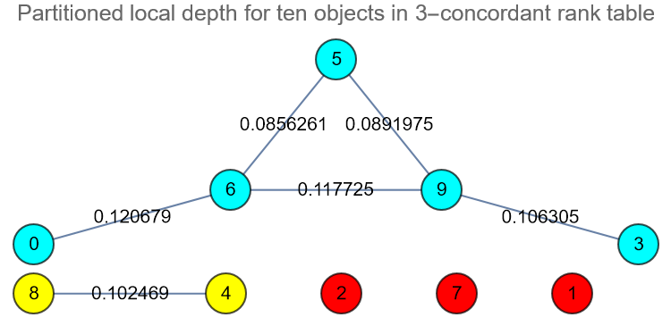
Rank-based linkage was inspired partly by partitioned local depth (PaLD) [9]. Figure 6 illustrates the cluster graph produced by PaLD, run against the same data from Table 1 as was used to illustrate rank-based linkage in Figure 3. In both cases, objects 0 and 6 form the most bonded pair, but objects 4 and 8 are not as strongly linked by PaLD as by rank-based linkage. To explain how the two methods differ, start by reframing the notion of conflict focus arising in the PaLD algorithm.
Definition 4.9.
Given an out-ordered digraph on , and undirected -NN graph ,
| (7) |
supplies the number of distinct for which the 2-simplex is -pertinent, and is not its source.
In other words counts the -pertinent 2-simplices in which is a 0-face, for each , where we take the in-sway to be zero when and are not mutual friends.
4.4.1. PaLD calculations
The essence of PaLD [9] is to construct an asymmetric cohesion as the sum of the reciprocals of the sizes (here ) over such that is the source in . The integer 2 refers to the inclusion of and in the count. When and are “close”, meaning that both and are small, then is relatively large, and therefore such a exerts more influence over the cohesion. The PaLD criterion for creating a link is that both and exceed a threshold defined in terms of the trace of the cohesion matrix; we omit details.
4.4.2. Partitioned NN local depth
In practical contexts, computing (7) entails cubic complexity in . For large numerical rounding errors alone make cohesion hard to compute, regardless of run time. To mitigate this complexity, [7] proposed an approximation to cohesion using -neighbors, called PaNNLD, which involves randomization of comparisons missing from the out-ordered digraph. Complexity is bounded by the sum of squares of vertex degrees in the undirected -NN graph.
4.4.3. Rank-based linkage
Rank-based linkage takes a different approach, motivated not only by complexity considerations, but more importantly by category theory: see Theorem 5.31. The calculation in Algorithm 1 uses uniform weighting, while taking so that only adjacent to in the undirected -NN graph participate in the sum. This gives complexity.
4.4.4. Rank-based linkage with weighting
One could compute the values (7) (at least on 0-cells of -pertinent 2-simplices) by inserting a couple of lines in Algorithm 1, assuming that has been initialized at zero for all pairs in . If the FirstElementIsSource predicate in Algorithm 1 returns true, then increment both and by 1 (since neither nor is the source of ). At the conclusion of Algorithm 1, both the functions and have been sufficiently evaluated.
Then there are two optional heuristics:
-
(1)
Return , i.e. the proportion of -pertinent 2-simplices containing in which is the source, as a measure of linkage.
-
(2)
Alternatively build a weighted, but still symmetric, version of in-sway: run Algorithm 1 again, but instead of incrementing by 1 in the inner loop, increment it by a weighted quantity such as if FirstElementIsSource returns true. The effect will be that when is “close” to or , then the 2-simplex exerts more influence on .
These weighted versions are not expected to satisfy Theorem 5.31, but are worth experimentation as a compromise between rank-based linkage and PaLD, with complexity.
5. Functorial properties of rank-based linkage
5.1. Overview
In this section, we present some functorial properties of the rank-based linkage process. The process from Section 2.7 can be broken into three stages, two of which are readily available in the literature. The first and most important step of the rank-based linkage process takes an out-ordered digraph and produces an edge-weighted graph. Next, the edge-weighted graph is pruned, subject to the weights of its edges. Lastly, the pruned graph is used to create a partitioned set.
Section 5.2 provides practical motivation for the rank-based linkage algorithm. Section 5.3 briefly discusses some constructions for digraphs, graphs, and edge-weighted graphs, which will be instrumental in building the rank-based linkage functor. Section 5.4 constructs the category of out-ordered digraphs, relating it back to traditional digraphs, and Section 5.5 constructs the key functor to edge-weighted graphs. Section 5.6 combines the steps together into the functor implementing ranked-based linkage from out-ordered digraphs to partitioned sets. Finally, Section 5.7 discusses the practical application of the rank-based linkage functor. Unlike Section 4, which assumes 3-concordance to simplify matters, calculations here apply to all out-ordered digraphs.
5.2. Practical motivation
Suppose a data scientist applies unsupervised learning to a collection of objects , with a specific comparator. Clusters are created based on a -neighbor graph on . Later further objects are added to the collection, giving a larger collection , still using the same comparator.
When unsupervised learning is applied a second time to , it is not desirable for the original set of clusters to “break apart” (see Section 5.3.2 for precise language); better for the elements of either to join existing clusters, or else form new clusters. To achieve this, we show that rank-based linkage is a functor from a category of out-ordered digraphs (Section 5.4) to a category of partitioned sets (Section 5.3.2). This desirable property is typically false for optimization-based clustering methods especially those which specify the number of clusters in advance, such as -means and non-negative matrix factorization.
Our presentation is modelled on Carlsson and Mémoli [12]’s functorial approach to clustering in the context of categories of finite metric spaces. Indeed the rank-based linkage algorithm arose as a consequence of the desire to emulate the results of [12]. The central technical issue is the definition of appropriate categories.
5.3. Definitions
In this section, we summarize some functorial relationships between categories of types of graphs. These relationships will be instrumental in proving that the process of rank-based linkage itself is also a functor from an appropriately constructed category. Some of these results are well-known in the literature or are folklore results that can be proven without undue difficulty. As such, some details will be omitted for brevity. The intrepid reader is invited to investigate further in [15, 22, 23, 24, 25, 28].
Section 5.3.1 briefly discusses the connections between graphs and digraphs, emphasizing the symmetric closure and its dual, the symmetric interior, both of which will be used in the construction of the rank-based linkage functor in Section 5.5. Section 5.3.2 considers the category of partitioned sets, which is presented differently, but equivalently, to the category of [12]. Section 5.3.3 concludes by introducing a category of edge-weighted graphs with edge-expansive maps, which will be the target of the rank-based linkage functor in Section 5.5.
Please note that throughout this discussion, 1-edges and directed loops will be allowed in graphs and digraphs, respectively.
5.3.1. Associations Between Graphs & Digraphs
To set notation, let and be the vertex and edge sets, respectively, of a digraph . Symmetric digraphs are a well-understood subclass of digraphs, which are deeply connected to (undirected) graphs. We summarize these connections here, and refer the intrepid reader to [22] for a more detailed exploration. Formally, we take the following definition and notation.
Definition 5.1 (Symmetric digraph, [25, p. 1]).
Let be the category of digraphs with digraph homomorphisms. A digraph is symmetric if implies . Let be the full subcategory of consisting of all symmetric digraphs, and let be the inclusion functor.
Recall that a subcategory is reflective if it is full and replete, and the inclusion functor admits a left adjoint [10, Definition 3.5.2]. Dually, a subcategory is coreflective if it is full and replete, and the inclusion functor admits a right adjoint [10, p. 119]. The category is a full subcategory of by definition, and repleteness is routine to demonstrate, so all that remains to consider is the existence of a left or a right adjoint. Recall that the symmetric closure of a binary relation is the smallest symmetric relation containing , and the symmetric interior of is the largest symmetric relation contained within [17, p. 305]. Below, both constructions are applied to the edge set of a digraph, which is merely a binary relation on the vertex set.
Definition 5.2 (Symmetric closure, [22, Definition 5.3]).
For a digraph , define the symmetric digraph by
-
•
,
-
•
.
Definition 5.3 (Symmetric interior, [22, Definition 5.5]).
For a digraph , define the symmetric digraph by
-
•
,
-
•
.
These two constructions correspond to the left and right adjoints of , respectively. Please note that the action of both adjoint functors is trivial on morphisms, which can be shown by means of the universal property of each.
For a graph , let and be its vertex and edge sets, respectively. An undirected graph can be thought of as a symmetric digraph, where each 2-edge is replaced with a directed 2-cycle and each 1-edge is replaced with a directed loop. This natural association is formalized in an invertible functor between the category of graphs and the category of symmetric digraphs.
Definition 5.4 (Equivalent symmetric digraph, [22, Definition 5.7]).
Let be the category of graphs. For , define by
-
•
,
-
•
,
-
•
.
5.3.2. Partitioned Sets
Observe that a digraph is merely a ground set equipped with a binary relation upon that ground set. When that relation is an equivalence relation, which partitions the ground set, we take the following definition.
Definition 5.5 (Partitioned set, [33, p. 2]).
A digraph is a partitioned set if is an equivalence relation on . Consequently, a partitioned set is a type of symmetric digraph. Let be the full subcategory of consisting of all partitioned sets, and let be the inclusion functor.
Realizing partitioned sets in this way shows that is a reflective subcategory of , where the reflector is the reflexive-transitive closure [41, p. 3:2] of the edge set. The equivalence relation generated in this process is the relation of connected components, where two vertices are related when there is a path from one to the other. The proof of the universal property is analogous to that of the symmetric closure and will be omitted for brevity.
Definition 5.6 (Reflexive-transitive closure).
For a symmetric digraph , define the partitioned set by
-
•
,
-
•
.
Let be the inclusion map.
Theorem 5.7 (Universal property).
If , there is a unique
such that .
As with and , the action of on morphisms can be shown to be trivial by means of the universal property above. Effectively, the left adjoint shows that digraph homomorphisms, and graph homomorphisms by means of the isomorphism , map connected components into connected components. That is, the connected components of the domain refine the components induced by the codomain.
In [12], partitioned sets were defined in terms of a partition on the ground set, and homomorphisms of partitioned sets were required to refine partitions through preimage. This “set system” representation of partitioned sets is isomorphic to the “digraph” representation that we have given above. The correspondence between equivalence relations and partitions is well-understood, so the only lingering question concerns the homomorphism conditions, which we shall show are equivalent. To that end, the following notation is taken for a partitioned set and :
-
•
is the equivalence class of in ;
-
•
is the set of all equivalence classes of .
Recall the following definition of refinement, which is integral to morphisms in the “set system” representation.
Definition 5.8 (Refinement, [3, p. 1]).
Let be a set and be partitions of . The partition refines if for all , there is such that .
Thus, we now show the equivalence of the two conditions.
Proposition 5.9 (Alternate morphism condition).
Let and be partitioned sets and . Then if and only if refines the family .
Proof.
If , there is such that . Let . If , then , so . Hence, , yielding . Therefore, .
Let satisfy that . If , then . There is such that . There is such that . As , , so . As is transitive, .
∎
While these two viewpoints are equivalent, we favor the “digraph” perspective due to the reflective relationship with symmetric digraphs presented in Theorem 5.7.
5.3.3. Edge-weighted Graphs
Edge-weighted graphs are not novel [30, p. 48], though we now consider a category of such objects. Formally, we take the following definitions for objects and morphisms.
Definition 5.10 (Expansive homomorphism).
Let be a graph. An edge-weight on is a function . The pair is an edge-weighted graph. For edge-weighted graphs and , an edge-expansive homomorphism from to is a function satisfying the following conditions:
-
•
(preserve adjacency) if , then ;
-
•
(expansive) if , then .
Let be the category of edge-weighted graphs with edge-expansive homomorphisms.
Much like [21, Definition 3.4.6], a traditional graph can be assigned a constant weight function, to which we give the following notation.
Definition 5.11 (Constant-weight functor).
Fix . For a graph , define the edge-weighted graph , where . For , define .
Routine calculations show that is a functor from to . However, while this functor may seem trivial, it admits a non-trivial right adjoint, where the edge set is trimmed only to those edges exceeding the fixed value . This is analogous to the unit-ball functor in functional analysis [1, 19, 20, 38, 39], and the proof is nearly identical.
Definition 5.12 (Cut-off operation).
Fix . For an edge-weighted graph , define the graph by
-
•
,
-
•
.
Let be defined by .
Theorem 5.13 (Universal property).
Fix . If , there is a unique such that .
Use of the universal property shows that acts trivially on morphisms. Moreover, is right adjoint to , which is the forgetful functor from to . Using the abbreviation “” for “ is left adjoint to ”, write , by analogy to [20, p. 176].
Theorem 5.14 (Secondary universal property).
If , there is a unique such that .
Lastly, there is a natural inclusion between the different cutoff functors. For an edge-weighted graph and , notice that . Thus, is a subgraph of , where potentially some edges have been removed. However, more can be said, and to do so, we take the following notation.
Definition 5.15 (Natural inclusion).
Say . For an edge-weighted graph , let be the inclusion map, and let .
As is bijective as a function, it is a bimorphism in . Moreover, a quick diagram chase with a morphism demonstrates that is a natural transformation from to . Likewise, a check shows that taken as a family, acts like an inverse system in the following way.
Proposition 5.16 (Inverse system).
If , then is a natural bimorphism from to . Moreover, if , then and .
5.4. Out-ordered Digraphs
In this section, we present a new class of graph-like structures, which will be used to codify the rank-based linkage process as a functor. The primary structure of study arises from Section 2: a set equipped with a neighborhood function and a partial order on each neighborhood. Formally, we take the definition below.
Definition 5.17 (Out-ordered digraph).
An out-ordered digraph is a triple satisfying the following conditions:
-
•
is the vertex set;
-
•
is the neighborhood function, i.e. is an edge if ;
-
•
is the neighborhood order, where is a partial order on for all .
To clarify the last bullet, means that is in the image of under , which is a set of ordered pairs of elements of .
Indeed, this structure is merely a digraph, where each out-neighborhood has been endowed with a partial order, ranking its out-neighbors. One can always impose this structure on a directed graph in a trivial way using the discrete ordering. However, the following example takes the form of the input to the rank-based linkage algorithm, as we saw in Section 2.6.
Example 5.18 (Edge-weighted digraph).
Let be a digraph and be a weight function on the edges. Define an out-ordered digraph by
-
•
(vertex set) ;
-
•
(out-neighborhood) ;
-
•
(weight order) for and , define iff one of the two conditions holds:
-
(1)
,
-
(2)
.
-
(1)
The homomorphisms between out-ordered digraphs have some natural qualities, mainly preserving the neighborhood and the order. However, we enforce two other conditions, which will be needed in Theorem 5.29. First, the morphisms must be injections, potentially adding elements but never quotienting them together. Second, any new elements that have been appended to a neighborhood must be ranked strictly farther than those already present. Effectively, this latter condition means that a neighborhood in the codomain is an ordinal sum [37, p. 547] of the image of the neighborhood in the domain with some new elements.
Definition 5.19 (Neighborhood-ordinal injection).
Given out-ordered digraphs and , a neighborhood-ordinal injection is a function satisfying the following conditions:
-
•
(neighborhood-preserving) for all , implies ;
-
•
(order-preserving) for all and , implies ;
-
•
(one-to-one) for all , implies ;
-
•
(ordinal sum)777 Notation: if , then is determined by for all and ,
implies for all .
While identity maps satisfy these conditions trivially, composition of morphisms is not trivial due to the ordinal sum condition.
Lemma 5.20 (Composition).
Let , , be out-ordered digraphs. Say is a neighborhood-ordinal injection from to , and is a neighborhood-ordinal injection from to . Then is a neighborhood-ordinal injection from to .
Proof.
It is routine to show that composition preserves neighborhoods, orders, and monomorphisms. To show the ordinal sum condition, let and satisfy that . Note that
Hence, consider the following two cases.
-
(1)
Assume that . Then, for all . If , then , so .
-
(2)
Assume that . Then, there is such that . If for some , then , contradicting that . Thus, . Therefore, for all , meaning for all . If for some , then , contrary to the standing assumption. Therefore, .
∎
Let be the category of out-ordered digraphs with neighborhood-ordinal injections. Using a constant weight in Example 5.18, every digraph can be given a neighborhood order. However, the reverse is also true, that the neighborhood order can be forgotten to return a traditional digraph. This forgetful functor will be instrumental in the next section to build the linkage functor. The proof of functoriality is routine.
Definition 5.21 (Forgetful functor).
For an out-ordered digraph , define the digraph by
-
•
,
-
•
.
For , define .
5.5. Linkage Functor
In this section, we construct the linkage functor, which takes an out-ordered digraph and returns an edge-weighted graph. Taking motivation from Section 2.2, we define different notions of “friendship”, which will be used to count elements toward the in-sway of Algorithm 1. Section 5.5.1 provides the definitions formally and ties each to the different graph constructions from Section 5.3.1. Section 5.5.2 uses these notions to construct the linkage graph of Section 2.7, and demonstrates that the construction is functorial.
5.5.1. Friendship Notations
Following the intuition of Section 2.2, we take the following formal definitions of “friend” and “mutual friends”. We also make the definition of “acquaintances”, which will be dual to and weaker than “mutual friends”.
Definition 5.22 (Friends).
Let be an out-ordered digraph. For , is a friend of if . Likewise, and are mutual friends if is a friend of and is a friend of . Dually, and are acquaintances if either is a friend of or is a friend of .
Each of these friendship notions in corresponds to a type of edge in . The proof of each characterization is routine and left to the reader. Recall the functor from Definition 5.4.
Lemma 5.23 (Characterization of friends).
Let be an out-ordered digraph and .
-
(1)
is a friend of iff .
-
(2)
and are mutual friends iff .
-
(3)
and are acquaintances iff .
Carrying the relationship methaphor forward, one can consider a “third-wheel”, someone who is looking at a relationship between two mutual friends from the outside. This idea can be compared to a parasocial relationship of a viewer of two content streamers, who commonly promote one another’s content.
To formalize this notion, let and be the mutual friends, and let be the outside observer. The most natural situation would be for and to be friends of , i.e. watches the content of both creators. However, it is possible that is also a creator, so or could frequent the content of . Thus, we must also consider the cases when is a friend of or , yielding the three cases listed in Figure 8. Such are the “voters” for in-sway from Section 2.7, and we take the following definition as the set of all such voters.
Definition 5.24 (Third-wheels).
Let be an out-ordered digraph. For , define the following set:
Please note that we purposefully omit the situation where is a friend of and , but and are not friends of . Returning to the content creator analogy, this is the case where does not frequent the content of either or , but they both frequent the content of . Such a would not vote, through methods such as likes or subscriptions, on the content of either or .
Moreover, the conditions defining the set are equivalent to those used to iterate Algorithm 1, noting that the underlying graph of is precisely the graph corresponding to the symmetric closure of .
Lemma 5.25 (Alternate characterization).
Let be an out-ordered digraph and fix . For all , if and only if the following conditions hold:
-
(1)
,
-
(2)
,
-
(3)
.
Consequently, .
The proof of the lemma is tedious, but routine, and provides an alternate characterization of the set : all that are acquaintances of both and , but have at least one of and as a friend.
5.5.2. Construction
At last, the in-sway for a pair of mutual friends can be computed as detailed in Algorithm 1, creating the linkage graph described in Section 2.7.
Definition 5.26 (In-sway weight function).
Let be an out-ordered digraph. For mutual friends , define the following set:
Define by and . For , define .
Our goal is to show that defines a functor from to . To that end, we prove a pair of technical lemmas, which will culminate in the functoriality of and a commutativity in Figure 9.
Lemma 5.27.
Let , , and . If and , then .
Proof.
Consider the following two cases.
-
(1)
Assume . Then, , so and . For purposes of contradiction, assume that . As is one-to-one, , which contradicts the strict inequality . Therefore, .
-
(2)
Assume . For purposes of contradiction, assume . Then there is such that . As is one-to-one, , contradicting that . Therefore, , so by the ordinal sum condition on .
∎
Lemma 5.28.
Let and . If and are mutual friends, then .
Proof.
If , then . By Lemma 5.25,
-
(1)
,
-
(2)
,
-
(3)
.
As is a functor, is a graph homomorphism from to . Thus, . Also,
Therefore, .
As , one has and . By Lemma 5.27, and . Hence, .
∎
Theorem 5.29 (Functoriality).
The maps define a functor from to . Moreover, .
5.6. Conclusion: the rank-based linkage functor
Finally, we assemble the functors from Figure 9 into a composite functor, which has the action of rank-based linkage.
Definition 5.30 (Rank-based linkage functor).
The functor implements the rank-based linkage algorithm from Section 2.7 precisely:
-
(1)
(Definition 5.26) computes the weighted linkage graph;
-
(2)
(Definition 5.12) prunes all edges with in-sway below ;
- (3)
Moreover, observe that by Theorem 5.29, , which returns the connected components of the linkage graph with no pruning of edges. Furthermore, the natural transformation passes from to , preventing the resulting partitions from breaking apart as the values of decrease. The work of this section may be concisely expressed as:
Theorem 5.31 (SUMMARY).
The rank-based linkage algorithm is the functor from the category of out-ordered digraphs to the category of partitioned sets.
5.7. Data science application
Return to the context of Section 5.2, where the scientist wishes to perform rank-based linkage on a superset of the set to which it was originally applied. How do neighborhood-ordinal injections (Definition 5.19) – the morphisms in the category of out-ordered digraphs – appear in this context?
Suppose the out-ordered digraph on objects was built on the -NN digraph. The out-ordered digraph on objects must be built on the -NN digraph where is large enough so that if is one of the -NN of in , then it must be one of the -NN of in . This will ensure that the injection is a neighborhood-ordinal injection, i.e. a morphism in the category of out-ordered digraphs.
Theorem 5.29 assures us that a pair of mutual friends in whose in-sway is at least will also have an insway at least when rank-based linkage is re-applied to . This ensures that if objects and are in the same component of , then they are also in the same component of . This is the functorial property of rank-based linkage.
6. Data merge: gluing ranking systems together
6.1. Data science context: merging sets of data objects
Principled methods of merging methods and data of unsupervised learning projects are rare, as the survey [32] shows. A categorical approach to merging databases is presented by Brown, Spivak & Wisnesky [11], but here we consider the unsupervised learning issue. Proposition 3.7 and Theorem 5.31 have direct application to pooling ranking systems on sets of data objects.
For the sake of concreteness, suppose Alice and Bob pursue bio-informatics in different laboratories. Alice has a collection of white mice which she uses to cluster a set of murine gene mutations, using comparator . Meanwhile Bob has a collection of brown mice which he uses to cluster a set of mutations, using comparator . Although their sets of mice are disjoint, the intersection of mutations may be non-empty.
6.2. Glued comparators
Alice and Bob meet at a data science conference. They decide to pool their data and comparators. Conversion between Alice’s and Bob’s formats is possible, enabling triplet comparisons
The first step is for Alice to include Bob’s brown mice, and for Bob to include Alice’s white mice, in the computations they perform with their respective comparators on their respective gene mutations999Technically speaking, this changes both the comparators; abuse notation by keeping the same symbols.. However they can do more: Alice and Bob can glue their comparators together, in a construction which category theorists will recognize as a pushout of two ranking systems.
All this requires is a compatibility condition: if are mutations in the intersection , then Alice and Bob agree on whether is more similar to than is to , when their respective comparators are applied to the combined mouse data. This condition appears as the first sentence of Definition 6.1.
Definition 6.1.
Suppose relations and are equivalent for . The glued comparator from comparators and is defined thus: agrees with for , and agrees with for .
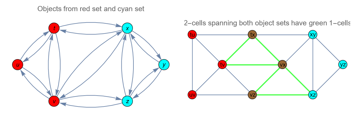
To understand Definition 6.1 in detail, let stand for elements of , shown in red in Figure 11, and let stand for elements of , shown in cyan. Figure 11 makes it clear that four types of voter triangle appear in :
| (8) |
The first and last of the voter triangles (8) can be understood entirely from the perspective of and of , respectively. However, the middle two in (8) involve interaction between the two ranking systems. For example, suppose and , giving orientations ; then the second voter triangle can be acyclic only if .
6.3. Pooling of nearest neighbor sets
Suppose the out-ordered digraph (Definition 2.1) induces an orientation on a simplicial complex and the out-ordered digraph induces an orientation on a simplicial complex , as in (6).
The simplicial complex associated with the glued comparator comes from an out-ordered digraph where neighborhoods must satisfy:
| (9) |
In practice, if and are based on -NN and -NN digraphs, respectively, then is based on a -NN digraph with respect to where is the least integer such that (9) holds. For this choice of , injections of the two ranking systems into their glued ranking system are morphisms in the category of out-ordered digraphs (Definition 5.19).
6.4. Sheaf property of 3-concordant ranking system enables pooling
Assume that Alice’s ranking system is 3-concordant, as is Bob’s ranking system . The sheaf property gives us tools to decide whether the glued comparator of Definition 6.1 is 3-concordant on the pooled data .
Proposition 3.7 has the following corollary, illustrated in Figure 11. The cost of checking for 3-concordance is much less than the cost of checking for absence of any cycles whatsoever in the fully concordant case.
Corollary 6.2.
A similar statement can be made concerning gluing of compatible 3-concordant sections of and to give a 3-concordant section of the simplicial complex above.
7. Sampling from 3-concordant ranking systems
Nothing more will be said about the theory of rank-based linkage. This section serves as a source of tools for generating synthetic data for experiments with rank-based linkage.
7.1. Why sampling is important
Machine learning algorithms applied to collections of points in uncountable metric spaces rarely admit any kind of statistical null hypothesis, because there is no uniform distribution on such infinite state spaces.
By contrast, the 3-concordant ranking systems on points, for a specific , form a finite set. Hence uniform sampling from such a set may be possible. Indeed Table 1. presents a uniform random 3-concordant ranking table , generated by rejection sampling. The statistics of links arising from rank-based linkage applied to provide a “null model”, to which results of rank-based linkage on a specific data set may be compared, in the same way that statisticians compare -statistics for numerical data to -statistics under a null hypothesis. With this in mind, we explore the limits of rejection sampling, and the opportunity for Markov chain Monte Carlo.
7.2. Ranking table
Concise representation of a 3-concordant ranking system on a set uses an ranking table , such as Table 1. Each row in table is a permutation of the integers . The entry is the rank awarded to object by the ranking based at object , taking . The advantage of this representation is that it requires only entries, and makes all enforcer triangles in the line graph acyclic automatically.
The condition for such a table to present a 3-concordant ranking system is that, whenever , then it is false that
| (10) |
for otherwise the 2-simplex would contain a 3-cycle, namely
Here we abuse notation, referring to the 1-simplex as simply .
7.3. Rejection sampling from ranking tables
When , a uniformly random 3-concordant ranking system can be found by sampling uniformly from the set of ranking tables, and rejecting if any of the tests (10) fails. Table 3 shows some results, and Table 1 came from our largest experiment.
| Number of objects | |||||
|---|---|---|---|---|---|
| Number of attempts | 50 | 2 | |||
| Mean # to success | 97.58 | 1,860.5 | 85,990 | ||
| Rate of 4-cycles | 1.4% | 1.3% | 1.2% | 1.2% | 1.2% or 0.7% |
7.4. Consecutive transposition in ranking tables
Consider a graph whose vertex set consists of the ranking systems on an -element set, each expressed in the form of a ranking table . Tables and are adjacent under if is obtained from by an operation called consecutive transposition, defined as follows. It is related to bubble sort and to Kendall tau distance [31].
Definition 7.1.
Given an ranking table , a consecutive transposition means:
-
(1)
Select a row for , and a rank between 1 and .
-
(2)
Identify elements and such that and , i.e. and are ranked consecutively according to the ranking at , so in particular .
-
(3)
Transpose and in the ranking at , meaning that we redefine and , so in particular .
Lemma 7.2.
If a ranking table presents a 3-concordant ranking system, then so does a ranking table obtained from by a consecutive transposition, unless
Proof.
Let be obtained from as explained in Definition 7.1. The enforcer triangles of form are still acyclic, because the rankings are unchanged except at ranks and . For , none of the rankings have changed so all enforcer triangles remain acyclic. The only voter triangle which has changed is , and the condition of the Lemma ensures that the 2-simplex does not contain a 3-cycle in Step 4. Hence none of the triangles in is a directed cycle. ∎
7.5. Random walk on 3-concordant ranking systems
We implemented a random walk on 3-concordant ranking systems using the following three steps:
-
(1)
Generate a random permutation of the 0-simplices. An acyclic orientation of the 1-simplices follows by taking whenever precedes in this random permutation. Initialize the ranking table using this orientation, which is concordant, and hence a fortiori 3-concordant.
- (2)
-
(3)
Repeat the last step many times.
Definition 7.3.
Random consecutive transposition with reflection at the 3-concordant boundary is the random walk defined above.
It would be ideal to terminate when “equilibrium” is attained, following Aldous and Diaconis [2] and hundreds of later papers which cite [2]. Unfortunately there is a difficulty. The Markov chain is not ergodic.
The graph on the 3-concordant ranking systems need not be connected.
Experiments revealed a counterexample when of a vertex in which is 3-concordant, without any 3-concordant neighbors in Hence at best the random walk will settle to equilibrium in the component determined by the initial orientation.
By contrast, acyclic orientations form a connected graph, where adjacency corresponds to a single edge flip. Fukuda, Prodon, & Sakuma [18] prove this by showing that, given two acyclic orientations , there is always some edge where and differ which can be flipped to give another acyclic orientation. This assertion no longer holds for 3-concordant orientations. A specific counterexample for is shown in Figure 12.
7.6. Open problems
7.6.1. The puzzle of the 4-cycles
Exhaustive enumeration revealed exactly 450 3-concordant ranking systems on the four points . Of these, there are 8 in which the 4-loop is a 4-cycle, in forward or reverse order. To make Table 1, we constructed uniform random samples of 3-concordant ranking systems for In these samples, when a 4-tuple was sampled uniformly at random, the proportion of 4-cycles (forwards or backwards) among corresponding 4-loops was not . Rather it seemed to decrease towards 1.2%. It seems that the ranking system induced on by a uniform 3-concordant ranking system on is not uniformly distributed among the 450 possibilities.
We suspect that the explanation for this is as follows. Let us choose a -concordant ranking system on points uniformly at random and consider extensions of it to a fifth point. It turns out that the expected number of possible extensions is ; on the other hand, if we consider only the systems that are not -concordant, the expected number is only . Accordingly one might expect that if we choose a -concordant ranking system uniformly on points, the probability of its restriction to a given set of points not being -concordant would be about , so that the probability of a given -loop would be about of this. This is roughly consistent with our observations; we do not expect this model to be exactly correct, because the events are not independent.
7.6.2. Intermediate sheaves
One might wish to consider a condition on orientations that is stronger than -concordance, but that nevertheless determines a sheaf. Is there a natural way of associating a nonzero sheaf to a simplicial complex such that for all , functorially with respect to inclusions of simplicial complexes, where the inclusions are proper for general ?
7.6.3. Products of Cayley graphs
Suppose we modify Definition 7.3 by skipping the check for the condition of Lemma 7.2. This unconstrained random walk is simply an -fold product of random walks on Cayley graphs; the Cayley graph for each factor is , where is the symmetric group on elements, and the generating set consists of permutations . For this Cayley graph, Bacher [5] has shown that the eigenvalues of the Laplacian satisfy
This tells us about the rate of convergence to equilibrium of the unconstrained random walk. The condition which forces reflection at the boundary of the 3-concordant ranking systems has the effect of inducing dependence between the factors in this product of random walks on copies of . Does convergence happen in about the same time scale. Is it steps, or , or some other rate?
7.6.4. Other Monte Carlo algorithm
Is there a better Markov chain Monte Carlo algorithm for sampling uniformly random 3-concordant ranking systems?
References
- [1] Jiří Adámek, Horst Herrlich, & George E. Strecker. Abstract and concrete categories: the joy of cats. Repr. Theory Appl. Categ., (17):1–507, ISBN:97804864693482006. Reprint of the 1990 original [Wiley, New York; MR1051419].
- [2] David Aldous & Persi Diaconis. Shuffling cards and stopping times. American Mathematical Monthly, 93, 333-348, 1986 http://dx.doi.org/10.1080/00029890.1986.11971821
- [3] A. Apostolico, C. S. Iliopoulos & R. Paige. An o() cost parallel algorithm for the single function coarsest partition problem. In Andreas Albrecht, Hermann Jung, and Kurt Mehlhorn, editors, Parallel Algorithms and Architectures, pages 70–76, Springer Berlin Heidelberg, 1987
- [4] Jonathan J. Azose & Adrian E. Raftery. Estimation of emigration, return migration, and transit migration between all pairs of countries. Proceedings of the National Academy of Sciences 116.1: 116-122, 2019 https://doi.org/10.1073/pnas.1722334116
- [5] Roland Bacher. Valeur propre minimale du laplacien de Coxeter pour le groupe symétrique. Journal of Algebra 167.2, 460-472, 1994
- [6] Jacob D. Baron & R. W. R. Darling. K-nearest neighbor approximation via the friend-of-a-friend principle. arXiv:1908.07645, 2019 https://doi.org/10.48550/arXiv.1908.07645
- [7] Jacob D. Baron, R. W. R. Darling, J. Laylon Davis, & R. Pettit. Partitioned -nearest neighbor local depth for scalable comparison-based learning. arXiv:2108.08864 [cs.DS], 2021 https://doi.org/10.48550/arXiv.2108.08864
- [8] Jacob D. Baron & R. W. R. Darling. Empirical complexity of comparator-based nearest neighbor descent. arXiv:2202.00517, 2022 https://doi.org/10.48550/arXiv.2202.00517
- [9] Kenneth S. Berenhaut, Katherine E. Moore, & Ryan L. Melvin. A social perspective on perceived distances reveals deep community structure. Proceedings of the National Academy of Sciences 119 (4), 2022 https://doi.org/10.1073/pnas.2003634119
- [10] Francis Borceux. Handbook of categorical algebra. 1 Basic category theory, volume 50 of Encyclopedia of Mathematics and its Applications. Cambridge University Press, Cambridge, 1994 https://doi.org/10.1017/CBO9780511525858
- [11] Kristopher Brown, David I. Spivak, & Ryan Wisnesky. Categorical Data Integration for Computational Science. arXiv:1903.10579 https://doi.org/10.48550/arxiv.1903.10579, 2019
- [12] G. Carlsson & F. Mémoli. Classifying Clustering Schemes. Found. Comput. Math. 13, 221–252 2013 https://doi.org/10.1007/s10208-012-9141-9,
- [13] Justin Michael Curry. Sheaves, cosheaves and applications. Thesis, University of Pennsylvania, 2014, arXiv:1303.3255, https://doi.org/10.48550/arxiv.1303.3255
- [14] R. W. R. Darling. rank-based-linkage Java API. To be released on GitHub, 2023
- [15] W. Dörfler & D. A. Waller. A category-theoretical approach to hypergraphs. Arch. Math. (Basel), 34(2):185–192, 1980 https://doi.org/10.1007/BF01224952
- [16] Martin Ester, Hans-Peter Kriegel, Jörg Sander, & Xiaowei Xu. Simoudis, Evangelos; Han, Jiawei; Fayyad, Usama M. (eds.). A density-based algorithm for discovering clusters in large spatial databases with noise.Proceedings of the Second International Conference on Knowledge Discovery and Data Mining (KDD-96). AAAI Press. pp. 226–231. 1996
- [17] C.A. Floudas & P.M. Pardalos. Encyclopedia of Optimization. Encyclopedia of Optimization. Springer US, ISBN:978-0-387-33624-4 2008
- [18] Komei Fukuda, Alain Prodon, & Tadashi Sakuma. Notes on acyclic orientations and the shelling lemma. Theoretical Computer Science 263, 9–16, 2001 https://doi.org/10.1016/S0304-3975(00)00226-7
- [19] K. R. Goodearl & P. Menal. Free and residually finite-dimensional -algebras. J. Funct. Anal., 90(2):391–410, 1990 https://doi.org/10.1016/0022-1236(90)90089-4
- [20] Marco Grandis. Categories, norms and weights. J. Homotopy Relat. Struct., 2(2):171–186, 2007
- [21] Will Grilliette. Scaled-free objects II. Ann. Funct. Anal., 6(3):216–261, 2015 http://dx.doi.org/10.15352/afa/06-3-18
- [22] Will Grilliette. Simplification for graph-like objects, arXiv:2012.08772v3 [math.CO], 2021 https://doi.org/10.48550/arXiv.2012.08772
- [23] Will Grilliette & Lucas J. Rusnak. Incidence hypergraphs: The categorical inconsistency of set-systems and a characterization of quiver exponentials, arXiv:1805.07670v2 [math.CO], 2019 https://doi.org/10.48550/arXiv.1805.07670
- [24] Pavol Hell. An introduction to the category of graphs. In Topics in graph theory (New York, 1977), vol.328 of Ann. New York Acad. Sci., pages 120–136. New York Acad. Sci., New York, 1979 http://dx.doi.org/10.1111/j.1749-6632.1979.tb17773.x
- [25] Pavol Hell & Jaroslav Nešetřil. Graphs and homomorphisms, volume 28 of Oxford Lecture Series in Mathematics and its Applications. Oxford University Press, Oxford, 2004 http://dx.doi.org/10.1093/acprof:oso/9780198528173.001.0001
- [26] Daniel Hernández Serrano & Darío Sánchez Gómez. Centrality measures in simplicial complexes: applications of topological data analysis to network science. Applied Mathematics and Computation vol. 382, 125331, 2020 https://doi.org/10.1016/j.amc.2020.125331
- [27] Java™ Platform, Standard Edition 20 API Specification. 2023 https://docs.oracle.com/en/java/
- [28] Mati Kilp & Ulrich Knauer. Graph operations and categorical constructions. Acta Comment. Univ. Tartu. Math., (5):43–57, 2001 http://dx.doi.org/10.12697/ACUTM.2001.05.04
- [29] Matthäus Kleindessner & Ulrike Von Luxburg. Lens depth function and k-relative neighborhood graph: versatile tools for ordinal data analysis. Journal of Machine Learning Research 18.1 1889-1940, 2017 https://doi.org/10.48550/arXiv.1602.07194
- [30] Joseph B. Kruskal. On the shortest spanning subtree of a graph and the traveling salesman problem. Proceedings of the American Mathematical Society, 7(1):48–50, 1956 http://dx.doi.org/10.1090/S0002-9939-1956-0078686-7
- [31] Ravi Kumar & Sergei Vassilvitskii. Generalized distances between rankings. Proceedings of the 19th International Conference on World Wide Web. 2010 http://dx.doi.org/10.1145/1772690.1772749
- [32] D. Lahat, T. Adali & C. Jutten. Multimodal data fusion: an overview of methods, challenges, and prospects. Proceedings of the IEEE, vol. 103, no. 9, pp. 1449-1477, 2015 https://doi.org/10.1109/JPROC.2015.2460697
- [33] Finnur Larusson. The homotopy theory of equivalence relations, arXiv:math/0611344v2 [math.AT], 2006 https://doi.org/10.48550/arXiv.math/0611344
- [34] Tom Leinster. Higher operads, higher categories, volume 298 of London Mathematical Society Lecture Note Series. Cambridge U. P., Cambridge, 2004 http://dx.doi.org/10.1017/CBO9780511525896
- [35] A. Mandal, M. Perrot, & D. Ghoshdastidar. A revenue function for comparison-based hierarchical clustering. arXiv preprint arXiv:2211.16459, 2022 https://doi.org/10.48550/arXiv.2211.16459
- [36] Bojan Mohar. Laplace eigenvalues of graphs – a survey. Discrete Mathematics, vol.109, Issues 1–3, pp 171-183, ISSN 0012-365X, 1992 https://doi.org/10.1016/0012-365X(92)90288-Q
- [37] Jose Morgado. On the closure operators of the ordinal sum of partially ordered sets. Indagationes Mathematicae (Proceedings), 64:546–550, 1961
- [38] J. Wick Pelletier & J. Rosický. Generating the equational theory of -algebras and related categories. In Categorical topology and its relation to analysis, algebra and combinatorics (Prague, 1988), pages 163–180. World Sci. Publ., Teaneck, NJ, 1989
- [39] J. Wick Pelletier & J. Rosický. On the equational theory of -algebras. Algebra Universalis, 30(2):275–284, 1993
- [40] Michaël Perrot, Esser Pascal, & Ghoshdastidar Debarghya. Near-optimal comparison based clustering. Advances in Neural Information Processing Systems 33, 19388-19399, 2022
- [41] Damien Pous. On the positive calculus of relations with transitive closure. In Rolf Niedermeier and Brigitte Vallée, editors, 35th Symposium on Theoretical Aspects of Computer Science (STACS 2018), volume 96 of Leibniz International Proceedings in Informatics (LIPIcs), pages 3:1–3:16, Dagstuhl, Germany. Schloss Dagstuhl–Leibniz-Zentrum für Informatik, 2018