Quantum localization corrections from the Bethe-Salpeter equation

Abstract

We investigate coherent matter wave transport in isotropic 3D speckle potentials by using the Bethe-Salper equation and the self-consistent theory of localization. This model constitutes an efficient tool to properly evaluate corrections to Boltzmann diffusion by taking into consideration quantum interference terms between the multiple-scattering paths. We calculate analytically and numerically the static current density, the density of states, the dipolar contribution and the reduced diffusion coefficient. Our results reveal that quantum corrections to diffusive transport, known as weak localization may not only lead to shift the above quantities but affect also the position of the mobility edge.

Keywords: Cold atoms, Optical speckle potentials, Bethe-Salper equation, Quantum localization correction, Quantum transport, Diffusion coefficient.

I Introduction

It has been established that the transport properties of a quantum particle in a disordered system are intrinsically determined by the interference of several scattering paths, which can lead to a spacial localization ref1 ; ref2 ; ref3 ; ref4 . The quantum particle then remains localized around its initial position, and it leads to a total suppression of transport, giving rise to arrest the diffusion and hence, cancel the conductivity ref5 ; ref6 .

Experimentally, the localization has been observed in many systems including light waves Wier ; Sche ; Sto ; Sch ; Lah , microwaves Dal ; Chab , sound waves Weav , electron gases ref24 , and coherent matter waves ref7 ; ref8 . Moreover, ultracold atoms open a new scenario for studying disorder-induced localization, due to high degree of interactions. Experimental observation of the Anderson transition of coherent matter waves in a disordered optical potential has been reported in Refs.ref7 ; ref8 . In three dimensions (3D), experimental observation of Anderson localization in matter waves of dilute Bose and Fermi gases in a speckle potential has been reported in ref10 ; ref9 .

One could argue that in disordered media the macroscopic transport properties namely diffusion, weak and strong localization, depend on the statistical properties of the disorder potential ref11 . The most interesting feature in the statistical properties of transport is the return probability to a given point in which all scattering paths are closed loops ref11 ; kunn . A weak localization comes from the fact that the probability of the wave to return to its initial position is possible through loop paths. Each loop can generate two multiple scattering paths along which exactly the same phase accumulates in successive scattering events results in constructive interferences of the matter wave. This coherent effect which is valid for any specific realization of the disorder potential leading to a diffusive transport for which the diffusion coefficient is reduced. On the other hand, if the disorder is strong the propagation of a coherent wave is stopped after a certain time in any dimension indicating that the diffusion coefficient vanishes. Therefore, the return probability decreases exponentially from a certain point in space with a characteristic length known as the localization length ref12 . Recently, quantum transport and Anderson localization of atomic matter waves in 3D anisotropic disordered potentials have been investigated in Piraud ; Piraud1 ; ref19 .

In the present paper, we use the Bethe-Salper equation and the self-consistent Born approximation to study the transport properties of ultracold atoms exposed to isotropic 3D speckle potentials far below the quantum degenerate regime (low densities). This model helps deal with the transport phenomenon of disordered BEC. We calculate in particular quantum corrections stemming from the interference effects known as weak localization to classical transport. Starting from the quantum kinetic theory, we calculate the current density and determine all relevant quantities such as the spectral function, the dipolar contribution, and the reduced diffusion coefficient that are necessary to describe the average diffusion process. Some useful analytic expressions are obtained in some limits.

Furthermore, we present our numerical solutions of the Bethe-Salpeter equation for the transport phenomenon of BEC subjected to a laser speckle potential. By means of the self-consistent Born approximation we evaluate iteratively the self-energy and the spectral function. This allows us to identify numerically the current density, the density of state, the fraction of the localized atoms and the diffusion coefficient. The main results emerging from this analysis is that corrections due to the interference effects may alter the overall behavior of these quantities and thus, affect the coherent transport regime. We show that the diffusion constant which depends on the atomic energy and on the disorder amplitude falls to zero due to the weak localization effects. The weak localization to the diffusion constant can be measured by releasing a confined atomic cloud and monitor its long-time spread inside the speckle field by time-of-flight or in-situ imaging techniques kunn . The increasing of the atomic energy leads to modify the position of the mobility edge. The most advantage of our method is that it does not require cutoffs to eliminate short wave paths that diverge even when scattering extends to infinite wave numbers in contrast to the theories of Refs.kunn ; Piraud . Our results provide new insights into the theory of Anderson localization and diffusion of matter wave in isotropic optical disorders.

The rest of the paper is organized as follows. In section II we introduce the basic concepts of quantum transport of matter waves in disordered media and present the Bethe-Salpeter equation and its the eigenfunction. We obtain also an analytic expression describing the quantum localization corrections for the diffusion constant in the case of an isotropic scattering. Section III is devoted to the numerical solutions of the Bethe-Salpeter equation for the transport phenomenon of BEC subjected to a laser speckle potential and compare them with classical regime. The current density and the reduced diffusion constant are also compued and compared with the analytical results. In section IV we present a brief summary.

II Coherent transport in a disordered medium

We consider a cloud of noninteracting cold atoms that is described by the single particle Hamiltonian $H=p^{2}/2m+V({\bf r})$, where $V({\bf r})$ is a static random potential introduced after the harmonic confinement in the transport directions has been switched off as in the experiments realized in ref7 ; ref8 . In such a regime of low densities, the evolution of the condensate is described by a linear time-dependent Schrödinger equation with a random potential. This latter is assumed to satisfy the following statistical properties: $\langle V(\mathbf{r})\rangle=0$, and $\langle V(\mathbf{r})V(\mathbf{r}^{\prime})\rangle=R(\mathbf{r}-\mathbf{r}^{\prime})$, where $\langle\bullet\rangle$ denotes the disorder ensemble average and $R(\mathbf{r}-\mathbf{r}^{\prime})$ is the disorder correlation function. In the following we deal with coherent transport of such noninteracting cold atoms in an isotropic disordered environment using the Bethe-Salpeter equation.
We set $\hbar=1$ throughout the manuscript.

II.1 Solutions of Bethe-Salpeter equation

Let us start by considering two particles of Green function $\phi_{\bf p,p^{\prime}}(\varepsilon,\Omega,\ {\bf q})$ which describes the probability density of matter wave in a disorder potential. We seek for the hydrodynamic expression which is defined as kunn ; Piraud ; ref15 :

$$\phi_{\bf p,p^{\prime}}(\varepsilon,\Omega,\ {\bf q})\equiv\overline{\langle{\bf p}_{+}|G(\varepsilon_{+})|{\bf p}^{\prime}_{+}\rangle\langle{\bf p}^{\prime}_{-}|G^{\dagger}(\varepsilon_{-})|{\bf p}_{-}\rangle},$$ (1)

where $G$ is the retarded Green operator, $\varepsilon_{\pm}=\varepsilon\pm\Omega/2$ , ${\bf p}_{\pm}={\bf p\pm q}/2$, ${\bf p^{\prime}_{\pm}=p^{\prime}\pm q}/2$ with ($q$ and $\Omega$ are the Fourier conjugate variables of space and time, respectively ref15 ). Our target is to analyze the behavior of the density diffusion for large distance and long times. We anticipate that at long time ($\Omega\rightarrow 0)$ and large distance $q\rightarrow 0$, the probability reads:

$$\phi_{\bf p,p^{\prime}}(\varepsilon,\Omega,\ {\bf q})=K\frac{L_{\varepsilon,{\bf p}}(\Omega,{\bf q})L_{\varepsilon,{\bf p^{\prime}}}(\Omega,{\bf q})}{-i\Omega+D(\varepsilon)q^{2}},$$ (2)

where $K$ is a normalized constant which will be determined later, $L_{\varepsilon,\bf p}(\Omega,{\bf q})$ is the eigenfunction of the Bethe-Selpeter equation associated with the hydrodynamic diffusion, and $D(\varepsilon)$ is the diffusion constant. The density diffusion $\phi_{\bf p,p^{\prime}}(\varepsilon,\Omega,\ {\bf q})$ is controlled by the Bethe-Salpeter equation, which can be formally written as Piraud ; Piraud1 :

$$\phi=\overline{G}\otimes\overline{G}^{\dagger}+\overline{G}\otimes\overline{G}^{\dagger}U\phi.$$ (3)

The first term in Eq. (3) represents the intensity propagation with uncorrelated disordered potential. The second term accounts for quantum corrections, involves the vertex function $U_{\bf p,p^{\prime}}$ which includes all correlations between different amplitudes in the density propagation. The Green function is defined as : $G({\bf p},\varepsilon)=[\varepsilon-\varepsilon_{\bf p}\ -\Sigma(\varepsilon,\ {\bf p})]^{-1}$, where $\varepsilon_{p}=p^{2}/2m$ is the kinetic energy of the particle, and $\Sigma(\varepsilon,{\bf p})$ is the self-energy which has already been examined in ref22 .

The product of the average propagators $\overline{G}^{\dagger}(\varepsilon_{-},{\bf p}_{-})\otimes\overline{G}(\varepsilon_{+},{\bf p}_{+})$ can be reformulated in momentum space by using the identity $\overline{G}^{*}*\overline{G}=\big{(}\overline{G}^{*}-\overline{G}\big{)}/\big{(}\overline{G}^{-1}-\overline{G}^{*-1}\big{)}$ kunn as:

$$\overline{G}(\varepsilon_{+},{\bf p}_{+})\overline{G}^{*}(\varepsilon_{-},{\bf p}_{-})=\frac{\overline{G}(\varepsilon_{+},{\bf p}_{+})\ -\overline{G}^{*}(\varepsilon_{-},{\bf p}_{-})}{\varepsilon_{-}-\varepsilon_{+}-({\bf p-\frac{1}{2}q})^{2}+({\bf p+\frac{1}{2}q})^{2}-\Sigma^{*}(\varepsilon_{-},{\bf p}^{-})+\Sigma(\varepsilon_{+},{\bf p}^{+})},$$ (4)

which can be rewritten in a compact form as:

$$\overline{G}(\varepsilon_{+},{\bf p}_{+})\overline{G}^{*}(\varepsilon_{-},{\bf p}_{-})=\frac{\Delta G_{\bf p}(\varepsilon,\Omega,\ {\bf q})}{-\Omega+2\,({\bf{p}\cdot\bf{q}})+\Delta\Sigma_{p}(\varepsilon,\Omega,{\bf q})},$$ (5)

where $\Delta G_{\bf p}(\varepsilon,\Omega,\ {\bf q})=\overline{G}(\varepsilon_{+},{\bf p}_{+})-\overline{G}^{*}(\varepsilon_{-},{\bf p}_{-})$, and $\Delta\Sigma_{p}(\varepsilon,\Omega,\ {\bf q})=\Sigma(\varepsilon_{+},{\bf p}_{+})-\Sigma^{*}(\varepsilon_{-},{\bf p}_{-})$.
This leads to the standard quantum kinetic equation:

$$\left[-\Omega+2({\bf p\cdot q})+\Delta\Sigma_{p}(\varepsilon,\Omega,\ {\bf q})\right]\phi_{\bf p,p^{\prime}}(\varepsilon,\Omega,\ {\bf q}) = \Delta G_{\bf p}(\varepsilon,\Omega,\ {\bf q})\delta_{\bf p,p^{\prime}}$$ (6)

$$+ \Delta G_{\bf p}(\varepsilon,\Omega,\ {\bf q})\sum_{p^{\prime\prime}}U_{\bf p,p^{\prime\prime}}(\Omega,\ {\bf q})\phi_{\bf p^{\prime\prime},p^{\prime}}(\varepsilon,\Omega,\ {\bf q}).$$

As shown by Vollhardt and Wölfle ref17 , the irreducible vertex $U_{\bf p,p^{\prime}}$ and the self-enegy $\Sigma_{\bf p}$ are related with each other through the Ward identity

$$\Delta\Sigma_{p}(\varepsilon,\Omega,\ {\bf q})=\sum_{p^{\prime}}\Delta G_{\bf p^{\prime}}(\varepsilon,\Omega,\ {\bf q})U_{\bf p^{\prime},p}(\varepsilon,\Omega,\ {\bf q}),$$ (7)

which describes the flux conservation.
Upon integrating over $p$, we obtain a simpler form of the continuity equation that describes the local conservation of the probability density

$$-\Omega\ P_{\bf p^{\prime}}(\varepsilon,\Omega,\ {\bf q})\ +{\bf q}\cdot{\bf j}_{\bf p^{\prime}}(\varepsilon,\Omega,\ {\bf q})\ \ =\Delta G_{\bf p^{\prime}}(\varepsilon,\Omega,\ {\bf q}),$$ (8)

where $\Omega=i\partial_{t}$ and ${\bf q}=i{\bf\nabla}$. This conservation equation which is similar to that obtained in Ref.kunn is valid for any initial distribution.

The probability density is written as: $P_{\bf p^{\prime}}(\varepsilon,\Omega,\ {\bf q})=\sum_{p}\phi_{\bf p,p^{\prime}}(\varepsilon,\Omega,\ {\bf q})$ and the current density reads: ${\bf j}_{\bf p^{\prime}}(\varepsilon,\Omega,\ {\bf q})=\sum_{p}2{\bf p}\cdot{\bf\phi}_{\bf p,p^{\prime}}(\varepsilon,\Omega,\ {\bf q})$.
One can easily check from Eq. (6) that

$$\sum_{pp^{\prime}}\phi_{\bf p,p^{\prime}}(\varepsilon,\Omega,\ q=0)=\frac{\sum_{p}\Delta G_{\bf p}(\varepsilon,\Omega,\ q=0)}{-\Omega},$$ (9)

where the factor $1/\Omega$ indicates that the total integrated density is conserved. The Ward identity (7) implies that $L_{\varepsilon,\bf p}=\Delta G_{\bf p}(\varepsilon)$ is a good choice for the eigenfunction at least for large distance $q\rightarrow 0$ and long time, $\Omega\rightarrow 0$. Therefore, we write

$$L_{\varepsilon,\bf p}(\Omega=0,{\bf q})=\Delta G_{\bf p}(\varepsilon,{\bf q})-\arrowvert G(\varepsilon,{\bf p})\rvert^{2}\Gamma({\bf p,q})+O(q^{2}),$$ (10)

where $\Gamma({\bf p,q})$ is supposed to be linear in $\bf{q}$ and can in isotropic media be written as: $\sim{\bf j}({\bf p})2({\bf p}\cdot{\bf q})$.
Replacing Eq.(2) into Eq.(6) for $\Omega=0$, one gets the following expression:

$$\left[2({\bf p\cdot q})+\Delta\Sigma_{p}(\varepsilon,{\bf q})\right]\big{[}\Delta G_{\bf p}(\varepsilon,{\bf q})\ -\arrowvert G({\bf p},\varepsilon)\rvert^{2}{\bf j}(\varepsilon,{\bf p})2({\bf p}\cdot{\bf q})\big{]}\ L_{\varepsilon,\bf p^{\prime}}({\bf q}) = D(\varepsilon)q^{2}\Delta G_{\bf p}(\varepsilon,{\bf q})\delta_{\bf p,p^{\prime}}$$

$$+ \Delta G_{\bf p}(\varepsilon,{\bf q})\sum_{p^{\prime\prime}}U_{\bf p,p^{\prime\prime}}(\varepsilon,{\bf q})\big{[}\Delta G_{\bf p^{\prime\prime}}(\varepsilon,{\bf q})$$

$$- \arrowvert G(\varepsilon,{\bf p^{\prime\prime}})\rvert^{2}{\bf j}(\varepsilon,{\bf p^{\prime\prime}})2({\bf p^{\prime\prime}}\cdot{\bf q})\big{]}L_{\varepsilon,\bf p^{\prime}}({\bf q}).$$

Expanding the identity (7) linearly in $q$ and inserting it into Eq.(II.1), we obtain

$$\left[2({\bf p\cdot q})+\Delta\Sigma_{p}(\varepsilon,{\bf q})\right]\Delta G_{\bf p}(\varepsilon,{\bf q})\ -\Delta G_{\bf p}(\varepsilon,{\bf q}){\bf j}({\bf p})2({\bf p}\cdot{\bf q}) = \Delta G_{\bf p}(\varepsilon,{\bf q})\Delta\Sigma_{\bf p}(\varepsilon,{\bf q})$$

$$- \Delta G_{\bf p}(\varepsilon,{\bf q})\sum_{p^{\prime\prime}}U_{\bf p,p^{\prime\prime}}(\varepsilon,{\bf q})\arrowvert G(\varepsilon,{\bf p^{\prime\prime}})\rvert^{2}{\bf j}(\varepsilon,{\bf p^{\prime\prime}})2({\bf p^{\prime\prime}}\cdot{\bf q}).$$

After some algebra, the quantum kinetic equation takes the form

$$2({\bf p\cdot q})+\sum_{p^{\prime\prime}}U_{\bf p,p^{\prime\prime}}(\varepsilon,\ {\bf q})\arrowvert G(\varepsilon,{\bf p^{\prime\prime}})\rvert^{2}{\bf j}(\varepsilon,{\bf p^{\prime\prime}})2({\bf p^{\prime\prime}}\cdot{\bf q})={\bf j}(\varepsilon,{\bf p})2({\bf p}\cdot{\bf q}).$$ (13)

The current density is immediately found to be given by Eq.(13) with ${\bf q}$ replaced by ${\bf p}$

$${\bf j}(\varepsilon,{\bf p})=1+\sum_{p^{\prime\prime}}\frac{{\bf p}^{\prime\prime}\ \cdot\ {\bf p}}{p^{2}}U_{\bf p,p^{\prime\prime}}(\varepsilon,0)\arrowvert G(\varepsilon,{\bf p^{\prime\prime}})\rvert^{2}{\bf j}(\varepsilon,{\bf p^{\prime\prime}}).$$ (14)

This result is independent of the small momentum ${\bf q}$ since in deriving Eqs. (II.1)-(14) we already kept only linear terms in ${\bf q}$, we therefore put ${\bf q}=0$ in $U_{\bf p,p^{\prime\prime}}(\varepsilon,\ {\bf q})$ ref17 ; VW ; ref18 . Equation (14) clearly shows that in lowest-order perturbation theory, $j(\varepsilon,{\bf p})=1$. The term $({\bf p}^{\prime\prime}\cdot{\bf p}/p^{2})U_{\bf p,p^{\prime\prime}}$ defines the cross section of all interference contributions in multiple scattering. Analytical solutions of Eq.(14) for 3D speckle potentials are shown in Appendix.

In order to find the eingenfunction of the Bethe-Salpeter equation, we employ the following transformation ref18 :

$$\Delta G_{\bf p}(\varepsilon,{\bf q})=G(\varepsilon,{\bf p+q}/2)\ -G^{*}(\varepsilon,{\bf p-q}/2)=2i\text{Im}G_{\bf p}(\varepsilon)\ +\ \frac{\partial\text{Re}\,G_{\bf p}(\varepsilon)}{\partial{\bf p}}\cdot{\bf q}.$$ (15)

Using the fact that

$$\frac{\partial\text{Re}\,G_{\bf p}(\varepsilon)}{\partial{\bf p}}\cdot{\bf q}=2\,{\bf p}\cdot{\bf q}\frac{\partial\text{Re}\,G_{\bf p}(\varepsilon)}{\partial p^{2}},$$

then introducing Eq.(15) into Eq. (10), one obtains for the eigenfunction of the Bethe-Salpeter equation

$$L_{\varepsilon,\bf p}({\bf q})=2i\,\text{Im}G_{\bf p}(\varepsilon)\ +2\ {\bf p}\cdot{\bf q}\frac{\partial\text{Re}\,G_{\bf p}(\varepsilon)}{\partial p^{2}}-\ \arrowvert G(\varepsilon,{\bf p})\rvert^{2}2\ ({\bf p}\cdot{\bf q}){\bf j}(\varepsilon,{\bf p}),$$ (16)

which admits an exact solution in linear order of $q$.

The spectrale function $\text{Im}G_{\bf p}(\varepsilon)$ contains all the information about the diffusion of the particles in a disordered medium. It is given by

$$-\text{Im}G_{\bf p}(\varepsilon)=\frac{\text{Im}\Sigma_{\bf p}(\varepsilon)}{\arrowvert{\varepsilon-\varepsilon_{\bf p}\ -\Sigma_{\bf p}(\varepsilon)}\rvert^{2}},$$ (17)

where the self-energy has the following form $\Sigma_{\bf p}(\varepsilon)=\sum_{\bf p^{\prime}}\ U_{\bf p,p^{\prime}}[\varepsilon-\varepsilon_{\bf p^{\prime}}-\Sigma_{\bf p^{\prime}}(\varepsilon)]^{-1}$ which is a negative function (represents the energy width of the spectral function). Thus,

$$\arrowvert G(\varepsilon,{\bf p})\rvert^{2}=\frac{\text{Im}G_{\bf p}(\varepsilon)}{\text{Im}\Sigma_{\bf p}(\varepsilon)}.$$ (18)

The scattering mean-free time is defined as:

$$\tau_{\bf p}(\varepsilon)=-\frac{\hbar}{2\ \text{Im}\Sigma_{\bf p}(\varepsilon)}.$$ (19)

Upon inserting Eqs.(17)-(19) into Eq.(16) and removing $-2i$, one finds:

$$L_{\varepsilon,\bf p}({\bf q})=-\text{Im}G_{\bf p}(\varepsilon)\ -i({\bf p}\cdot{\bf q})\ \gamma({\bf p},\varepsilon),$$ (20)

where

$$\gamma(\varepsilon,{\bf p})=\ \text{Im}G_{\bf p}(\varepsilon)\,2\tau_{\bf p}(\varepsilon){\bf j}(\varepsilon,{\bf p})\ -\frac{\partial\text{Re}\,G_{\bf p}(\varepsilon)}{\partial p^{2}}\ +O(q^{2}),$$ (21)

is called the dipolar contribution which generates the flow of energy and thus, provides corrections that support a current density. The solution of the Bethe Salpeter equation $L_{\varepsilon,\bf p}({\bf q})$ at small $q$ is governed by the spectral function ($A(\varepsilon,{\bf p})=-\text{Im}G_{\bf p}(\varepsilon)/\pi$).

Finally, the normalization constant $K$ can be determined by matching Eq. (9) and Eq.(2) for $q=0$. This yields

$$K\sum_{pp^{\prime}}\frac{\text{Im}G_{\bf p}(\varepsilon)\text{Im}G_{\bf p^{\prime}}(\varepsilon)}{-i\Omega}=\frac{\sum\limits_{p}2i\text{Im}G_{\bf p}(\varepsilon)}{-\Omega},$$ (22)

we thus, immediatly deduce that

$$K=\frac{2}{\sum\limits_{p}-\text{Im}G_{\bf p}(\varepsilon)}.$$ (23)

Replacing the resulting constant (23) into Eq.(2), one gets for the quantum propability

$$\phi_{\bf p,p^{\prime}}(\Omega,\ {\bf q})=\frac{2}{\sum\limits_{p}-\text{Im}G_{{\bf p}}(\varepsilon)}\frac{L_{\varepsilon,\bf p}({\bf q})L_{\varepsilon,\bf p^{\prime}}({\bf q})}{-i\Omega\ +\ Dq^{2}},$$ (24)

which has a diffusion pole according to kunn ; Piraud ; ref18 . The sum $\sum\limits_{p}-\text{Im}G_{\bf p}(\varepsilon)$ is linked to the density of states per unit volume $\rho(\varepsilon)$ as: $\sum\limits_{p}-\text{Im}G_{\bf p}(\varepsilon)=\pi\rho(\varepsilon)$.
For $p\longrightarrow\infty$, $\text{Im}\Sigma_{\bf p}(\varepsilon)$ vanishes, we then expect that $j(p)\longrightarrow 1$. The dipolar contribution $\gamma(\varepsilon,{\bf p})$ has the following form

$$\gamma_{0}(\varepsilon,{\bf p})=\ \ \arrowvert G(\varepsilon,{\bf p})\rvert^{2}\ -\frac{\partial\text{Re}\,G_{\bf p}(\varepsilon)}{\partial p^{2}}.$$ (25)

Here $\gamma_{0}(\varepsilon,{\bf p})$ describes multiple scattering as a sequence of scattering events where both retarded and advanced amplitudes travel along the same path. When $p\longrightarrow\infty$, the kinetic energy of the atoms exceeds the exitation potential, a large isotropic waves travel without feeling the disorder effect ref15 ; kunn .

II.2 Diffusion constant from quantum localization corrections for isotropic scattering

We now concentrate on the calculation of the diffusion constant using the quantum kinetic equation derived in the previous section. Let us write the expression of the current density

$${\bf j}_{\bf p^{\prime}}(\varepsilon,\Omega,\ {\bf q})=2\sum_{p}\ {\bf{p}\cdot\phi_{\bf p,p^{\prime}}}(\varepsilon,\Omega,\ {\bf q}).$$ (26)

Incorporating $\phi_{\bf p,p^{\prime}}$ from Eq.(24) into ${\bf j}_{\bf p^{\prime}}(\varepsilon,\Omega,\ {\bf q})$, we find

$${\bf j}_{\bf p^{\prime}}(\varepsilon,\Omega,\ {\bf q})=\frac{2}{\pi\rho(\varepsilon)}\frac{L_{\varepsilon,\bf p^{\prime}}({\bf q})}{-i\Omega\ +\ Dq^{2}}\sum_{p}2{\bf p}\ L_{\varepsilon,\bf p}({\bf q}).$$ (27)

Inserting the corrections manifesting in $L_{\varepsilon,\bf p}({\bf q})$ into Eq. (27), we obtain

$${\bf j}_{\bf p^{\prime}}(\varepsilon,\Omega,\ {\bf q})=\frac{2}{\pi\rho(\varepsilon)}\frac{L_{\varepsilon,\bf p^{\prime}}({\bf q})}{-i\Omega+\ Dq^{2}}i\ {\bf q}\ \ \frac{2}{3}\sum_{p}\bigg{[}-\ \text{Im}G_{\bf p}(\varepsilon)2\tau_{\bf p}(\varepsilon){\bf j}(\varepsilon,{\bf p})p^{2}\ -\ p^{2}\frac{\partial\text{Re}\,G_{\bf p}(\varepsilon)}{\partial p^{2}}\bigg{]}.$$ (28)

The factor $(1/3)$ that appears in Eq. (28) comes from the angular integral.

The probability density is defined as:

$$P_{\bf p^{\prime}}(\varepsilon,\Omega,\ {\bf q})=\sum_{p}\phi_{\bf p,p^{\prime}}(\varepsilon,\Omega,\ {\bf q})=2\ \frac{L_{\varepsilon,\bf p^{\prime}}({\bf q})}{-i\Omega\ +\ Dq^{2}}.$$ (29)

According to Fick’s law, which relates the diffusive flux to the concentration gradient in the diffusive regime ($\Omega,{\bf q}\rightarrow 0$), ${\bf j}_{\bf p^{\prime}}(\varepsilon,\Omega,\ {\bf q})=i\ {\bf q}D(\varepsilon)P_{\bf p^{\prime}}(\varepsilon,\Omega,\ {\bf q})$, the diffusion constant is extracted as:

$$D(\varepsilon)\ =\ \frac{1}{\pi\rho(\varepsilon)}\frac{2}{3}\sum_{p}p^{2}\left(-\text{Im}G_{\bf p}(\varepsilon)2\tau_{\bf p}(\varepsilon){\bf j}(\varepsilon,{\bf p})\ -\ p^{2}\frac{\partial\text{Re}\,G_{\bf p}(\varepsilon)}{\partial p^{2}}\right).$$ (30)

This equation is appealing since it includes weak localization corrections. In the regime of a weak disorder, $\text{Im}G_{\bf p}(\varepsilon)$ is strongly peaked near $p=\sqrt{\varepsilon}$, yielding $\pi\rho(\varepsilon)\approx\sqrt{\varepsilon}/(4\pi)$. Therefore, $D(\varepsilon)$ reduces to:

$$D(\varepsilon)=\frac{4\pi}{\sqrt{\varepsilon}}\frac{2}{3}\frac{4\pi}{(2\pi)^{3}}\pi\int_{0}^{\infty}dpp^{4}\delta(\varepsilon-p^{2})2\tau_{\bf p}(\varepsilon){\bf j}({\varepsilon,\bf p}).$$ (31)

Keeping in mind that the second term is negligible, we find: $D(\varepsilon)=4\varepsilon\,j(\sqrt{\varepsilon})\tau_{p=\sqrt{\varepsilon}}/3$. Asuming that $j(\sqrt{\varepsilon})=1$ at large $\varepsilon$, we recover the familiar expression for classical wave namely $D(\varepsilon)=v^{2}\tau^{*}/3$ Shap ; Boudj , where $v$ is the wave velocity, and $\tau^{*}$ is a transport mean free time which is straightforwardly associated with the transport mean path $\ell^{*}$ via $\tau^{*}=\ell^{*}/v$.

In the next section, we will discuss the critical regime of transition by numerically solving the above Bethe-Salper equation.

III Numerical results

In this section, we solve numerically the Bethe-Salpeter equation for the transport phenomenon of BEC subjected to a laser speckle potential. To do so, we apply the self-consistent Born approximation to calculate the self-energy which is the key factor of the diffusion. The current density $j(p)/p$ is computed iteratively, and then insert the result into Eq.(30) to obtain the diffusion coefficient. The number of required iterations for convergence is $100$ iterations which are enough to obtain the desired solution Boudj .

From now on, all energies, including $\Sigma$, are expressed in units of the quantum correlation energy $\varepsilon_{\sigma}=1/(2m\sigma^{2})$ with $\sigma$ being the correlation length, momenta are expressed as $p=k$, where the de-Broglie wave number $k$ is scaled in units of $1/\sigma$ (we recall that $\hbar$=1). We choose a constant value of the disorder amplitude $(V_{R}=0.5\varepsilon_{\sigma})$ for which the condition of a perturbative disorder to be valid $\varepsilon_{k}\gg V_{R}^{2}/\varepsilon_{\sigma}$ delande .

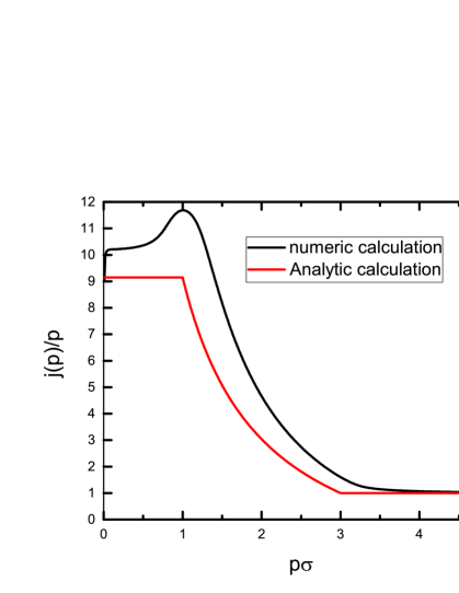
Figure 1: Static current density $j(p)/p$ as a function of $p\sigma$ for $\varepsilon_{c}=0$.

In Figure 1 we report the numerical and analytical results of the current density $j(p)/p$ as a function of the scaled wave number $p\sigma$. We see that the current density reaches its maximum at $p\sigma\lesssim 1$, then it decreases and becomes constant for large momenta. The analytical results and the numerical simulation diverge from each other notably for small momenta. A closer look at the same figure shows that the numerical simulation predicts a hump in the current density at $p\sigma\sim 1$, indicating that more atoms can participate in the multiple scattering. These atoms are dephazing from their initial positions most probably due to the effect of a weak localization. Both methods show that the current diffusion converge to $1$ at very large momentum $(p\rightarrow\infty)$. In such a regime weak localization corrections disappear and a classical diffusion takes place (see also Eq. (14)).

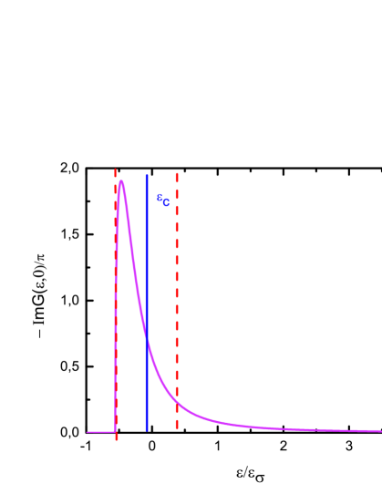
Figure 2: Spectral function for $p=0$ and $V_{R}=0.5\varepsilon_{\sigma}$.

To calculate the spectral function, we solve numerically Eq. (17). The results are shown in Figure 2. We observe the appearance of a peak at $\varepsilon=-0.5\varepsilon_{\sigma}$. The width half height of this peak $\Delta\varepsilon=0.4\varepsilon_{\sigma}$ is inversely proportional to the mean free time of the atoms in speckle. At low energies, the relevant parameter of localization is the typical length $\ell_{c}$ which is associated with a typical momentum $k_{c}=\sqrt{2m\varepsilon_{c}}$. Note that the width of the spectral function at $\varepsilon=\varepsilon_{c}$ is of the order of $\ell_{c}\sim\sigma/(V_{R}/\varepsilon_{\sigma})^{2}$ref23 . In our case, we find $\ell_{c}\approx 4\sigma$. From the same figure we see that the mobility edge is located at $\varepsilon_{c}/\varepsilon_{\sigma}=-0.04$ which implies that $k_{c}/k_{\sigma}=0.2$. In the limit of weak disorder, we find $k_{c}\ell_{c}=0.8$ satisfying the celebrated Ioffe-Regel criterion namely, $(k_{c}\ell_{c}\sim 1)$ BART . For $\ell_{c}\gg 4\sigma$, the density atomic exceeds the optical potential which means that $\ell_{c}$ varies faster than the modulations of the speckle $\sigma$. In such a situation we fall to a classical diffusion.

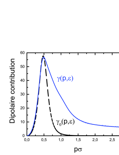
Figure 3: Dipolar contributions $\gamma(p,\varepsilon)$ and $\gamma_{0}(p,\varepsilon)$ for $\varepsilon/\varepsilon_{\sigma}=-0.1$. Here $\gamma(p,\varepsilon)$ is associated with coherent matter wave transport (in the presence of the quantum corrections) and $\gamma_{0}(p,\varepsilon)$ corresponds to the incoherent matter wave transport (in the absence of the quantum corrections).

The solution of Bethe-Salpeter equation for the dipolar contribution in the regime of coherent matter wave transport (i.e. in the presence of the quantum corrections, $\gamma(\varepsilon,p)$) and for the incoherent matter wave transport (i.e. classical regime, $\gamma_{0}(p,\varepsilon)$ is captured in figure 3. We see that the two curves are almost indistinguishable, yielding an excellent agreement in the region $p\sigma<0.5$. Whereas for $p\sigma>0.5$, the curves diverge form each other (the width of quantum particles curve is broadened) due to the enhancement of the correlations induced by weak localization. The narrow spectrum in the classical regime indicates the absence of quantum correlation effects. In the presence of the quantum corrections, the energetic atoms are shifted by the interference giving rise to increase the intensity of the dipolar contribution results in a large anisotropic momentum because of their deviations by the disorder effect Piraud . Given that $p\sigma$ equivalent to $\upsilon_{p}/\upsilon_{\sigma}$, where $v_{\sigma}=1/\ m\sigma$, we find that the dipolar contribution $\gamma(\varepsilon,p)$ is dominated by atoms with velocity $v_{\sigma}=0.66/m\sigma$. We detect on the other hand a fraction of atoms faster than $v_{\sigma}=1.11/m\sigma$ contributing to the multiple diffusion. Our results show a large spectrum in $\gamma(\varepsilon,p)$ compared to that obtained in Ref.ref18 since we take into account higher-order contribution to the current density $j(p)$.

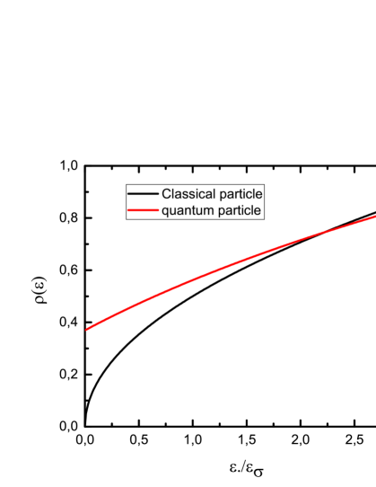
Figure 4: The density of states per unit of volume as a function of $\varepsilon/\varepsilon_{\sigma}$ for $p=0$. In the classical diffusion the density of states is given as: $\rho(\varepsilon)=4\pi\delta(\varepsilon-\varepsilon_{p})$.

These quantum corrections have an important impact on the distribution of waves packet. This can be seen in the density of states $\rho(\varepsilon)=\int\text{ Im}G(\varepsilon,p)d{\bf p}/(2\pi)^{3}$ which measures the average number of states in the random medium per unit of volume. Figure 4 depicts that at energies $\varepsilon\ll\varepsilon_{\sigma}$, the probability is small but finite. Our numerical calculation predicts that around $38\%$ of atoms are localized due to the interference effects. Here the fraction of localized atoms is given by $f_{\text{loc}}\approx\int_{-\infty}^{\varepsilon_{c}}\ d\varepsilon\text{ Im}G(\varepsilon,p=0)$ ref23 . At higher energies, the probability grows with the energy. In such a situation, one has $\text{Im}G(\varepsilon,p)=-\pi\delta(\varepsilon-\varepsilon_{p})$, hence the atoms do not feel the disorder potential and the system attains the classical diffusion. Consequently, the density of states behaves like the free-space expression $\rho(\varepsilon)\sim\varepsilon^{1/2}$, where the dispersion relation reads $\varepsilon=p^{2}/2m$ (see black line in figure 4). It is clear that the two curves (quantum and classical) cross with each other at $\varepsilon\simeq 2.25\varepsilon_{\sigma}$ pointing out that the atoms diffuse in a classical way at energies $\varepsilon\gtrsim 2.25\varepsilon_{\sigma}$.

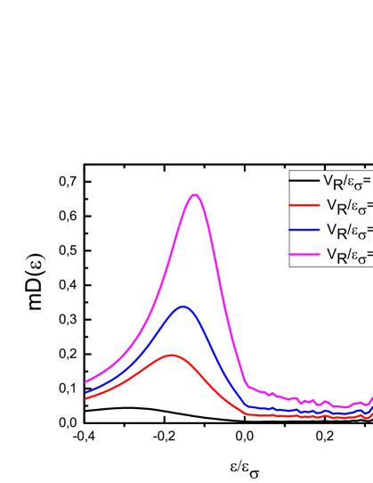
Figure 5: Diffusion coefficient as a function of the energy for several values of the disorder amplitude and for $p=0$.

In Figure 5, we plot the diffusion constant as a function of the energy for different disorder amplitudes. Our results reveal that the diffusion coefficient $mD(\varepsilon)$ reaches its maximum at negative energies for any disorder amplitude, then it decreases when the energy becomes close to zero. Such a decay in the diffusion coefficient which depends also on the scattering amplitude as is seen in figure 5, is due to the weak localization effects induced by the fluctuations caused by the number of scatterers.

Figure 6: Standard deviation of the diffusion coefficient in a critical regime for $V_{R}/\varepsilon_{\sigma}=0.5$.

Let us discuss more profoundly the transport properties from diffusion coefficient. To this end, we use the standard deviation to approach the transition point. Figure 6 shows three distinct regions. In the first region, $-0.12<\varepsilon/\varepsilon_{\sigma}<-0.04$, $mD(\varepsilon)$ decreases rapidly with the energy until it attains the mobilty edge $\varepsilon_{c}=-0.04\varepsilon_{\sigma}$. The situation is different in the second region, $-0.04<\varepsilon/\varepsilon_{\sigma}<0$, where the diffusion coefficient increases linearly. A similar behavior holds true for a Gaussian disorder potential ref23 . In this region, the states cease to extend over the disorder potential and thus delocalize. In the third interval $\varepsilon>0$ and for small energies, $mD(\varepsilon)$ is saturated to a constante value ($mD(\varepsilon)\approx 0.25$) owing to the weak localization effects. This phenomenon is important because the wave transport is quite sensitive to large momentum which leads to increase the interferences between scattered atoms evoking a deviation of fast atoms from its initial position and hence reducing the constant diffusion. This is in stark contrast with the Dirac-peaks potential ref24 , where the atoms are insensitive to the disorder effects. Note that in the anisotropic case, the diffusion coefficient increases in power law in the limit of low energies while it behaves as $D\propto\varepsilon^{5/2}$ at higher energies Piraud .

IV Conclusion

In this paper, we examined the transport and localization of matter waves in isotropic 3D speckle potentials using the Bethe-Salper equation and the self-consistent theory of Anderson localization. We calculated in particular the fundamental transport quantities such as the current intensity, the dipolar contribution, the density of states, the spectral function, and the reduced diffusion constant. We found that these quantities deviate from their classical counterpart due to corrections arising from multiple scattering of matter waves. At low energy, our numerical calculations predict that the weak localization corrections increase the probability density and may shift the dipolar contribution. The reduction of the diffusion constant which depends on the scattering amplitude signals the occurrence of weak localization effects. Our results pointed out also that the diffusion process continues with the initially fast atoms until the transport means path becomes of the order of the wavelength of the condensate.

CRediT author statement

Afifa Yedjour: Conceptualization, Methodology, Software, Data curation, Writing- Original draft preparation.
Abdelaali Boudjemaa: Visualization, Investigation, Writing-Review and Editing

V Appendix

In this appendix we derive an explicit expression for the density current in the case of a 3D laser speckle potential produced by diffraction which is widely used with quantum gases experiments, its correlation function is given by $\langle U({\bf R})\rangle=V_{R}^{2}\mathrm{sinc}^{2}(R/\sigma)$, where $V_{R}$ is the amplitude disorder. For $V_{R}\rightarrow\infty$ and $\sigma\rightarrow 0$, the speckle potential reduces to the uncorrelated white-noise random potential. In Fourier space one can write:

$$U_{\bf p,p^{\prime}}=V_{R}^{2}\int d{\bf R}\sum_{\bf p^{\prime}}\dfrac{\sin^{2}\left(R/\sigma\right)}{\left(R/\sigma\right)^{2}}e^{i({\bf p}-\ {\bf p}^{\prime})\cdot{\bf R}}.$$ (32)

Inserting $U_{\bf p,p^{\prime}}$ into Eq. (14) and using the fact that $\sum_{\mathbf{p^{\prime}}}\equiv\int d{\bf p^{\prime}}/(2\pi)^{3}$, one finds

$$j(\varepsilon,{\bf p})=1+\frac{V_{R}^{2}}{(2\pi)^{3}}I({\bf p,\ p^{\prime}})\arrowvert G(\varepsilon,{\bf p^{\prime}})\rvert^{2}j(\varepsilon,{\bf p^{\prime}}),$$ (33)

where

$$I({\bf p,\ p^{\prime}})=\int d{\bf R}\int d{\bf p}^{\prime}\frac{{\bf p}\cdot\ {\bf p}^{\prime}}{p^{2}}\dfrac{\sin^{2}\left(R/\sigma\right)}{\left(R/\sigma\right)^{2}}e^{i({\bf p}-\ {\bf p}^{\prime})\cdot{\bf R}}.$$ (34)

Setting $\int d\hat{p^{\prime\prime}}=\ dp^{\prime\prime}p^{\prime\prime 2}$, then the integral in momentum space becomes

$$\int\frac{d\hat{p^{\prime}}}{4\pi}({\bf p}\ \cdot\ {\bf p}^{\prime})e^{i({\bf p}-\ {\bf p}^{\prime})\cdot{\bf R}} = {\bf p}\cdot\frac{1}{p^{\prime}}e^{\ i\ {\bf p}\cdot{\bf R}}\cdot i\frac{\partial}{\partial{\bf R}}\int d\hat{p^{\prime}}e^{-\ i\ {\bf p}^{\prime\prime}\cdot{\bf R}}$$

$$= {\bf p}\cdot\frac{e^{i\ {\bf p}^{\prime}\cdot{\bf R}}}{p^{\prime}}i\frac{\partial}{\partial{\bf R}}\mathrm{sinc}(p^{\prime}\ R)$$

$$= \frac{\hat{p}.\hat{R}}{R}e^{i\ {\bf p}\cdot{\bf R}}i\frac{\partial}{\partial p^{\prime}}\mathrm{sinc}(p^{\prime}\ R).$$

Now the integral over $R$ can be evaluated as:

$$\int\frac{d\hat{R}}{4\pi}\ \hat{R}\ e^{i{\bf p}\cdot{\bf R}} = \frac{1}{R}\frac{1}{i}\frac{\partial}{\partial\ p}\int\frac{d^{3}\hat{R}}{4\pi}e^{\ i\ {\bf p}\cdot{\bf R}}=\frac{\hat{p}}{R}\frac{1}{i}\frac{\partial}{\partial\ p}\mathrm{sinc}(p\ R).$$ (36)

With this, Eq (34) can be rewritten as:

$$I(p,\ p^{\prime})=4\pi\frac{\partial}{\partial\ p}\frac{\partial}{\partial\ p^{\prime}}\int_{0}^{\infty}dR\,\mathrm{sinc}^{2}\left(\dfrac{R}{\sigma}\right)\mathrm{sinc}(p\ R)\ \mathrm{sinc}(p^{\prime}\ R)=4\pi\frac{\partial}{\partial\ p}\frac{\partial}{\partial\ p^{\prime}}\frac{1}{pp^{\prime}}\ K(p,p^{\prime}),$$ (37)

where

$$K(p,p^{\prime})=\int_{0}^{\infty}dR\ \mathrm{sinc}^{2}\left(\dfrac{R}{\sigma}\right)\left(\frac{\sin p^{\prime}R}{R}\right)\left(\frac{\sin R}{R}\right).$$ (38)

Putting

$$M(p,p^{\prime})=\frac{\partial}{\partial\ p}\ \frac{\partial}{\partial\ p^{\prime\prime}}\ K(p,p^{\prime})=\int_{0}^{\infty}\ dR\,\mathrm{sinc}^{2}\big{(}R/\sigma\big{)}\cos(p\ R)\ \cos(p^{\prime\prime}\ R).$$ (39)

Then employing the relation $\int_{-\infty}^{+\infty}dRe^{iqR}/R=\pi\Theta(q)$, we obtain:

$$M(p,p^{\prime})\ =\ \frac{\pi\sigma}{16}\left[2\ -\ p\ -\ p^{\prime}\ -\ 2\lvert p\ -\ p^{\prime}\rvert\ +\lvert p\ +\ p^{\prime}\ -\ 2\rvert\ \ +\ \lvert 2\ -\ p\ +\ p^{\prime}\rvert\ \ +\ \lvert 2\ +\ p\ -\ p^{\prime}\rvert\ \right].$$ (40)

Upon substituting Eq.(40) into Eq.(37), we find

$$I(p,p^{\prime})\ =\ \frac{4\pi^{2}\sigma}{16}\left[I_{1}\ +\ I_{2}\ +\ I_{3}\ +\ I_{4}\ \right],$$ (41)

where

$$I_{1}=2\ \frac{p\ +\ p^{\prime}\ -\ 2}{p^{2}p^{\prime 2}}\left(-p^{2}\ -\ p^{\prime 2}\ +\ pp^{\prime}\ +2\ +p\ +\ p^{\prime}\ \right)\left(\Theta\left(p\ +\ p^{\prime}\ -\ 2\right)\ -\ 1\right),$$

$$I_{2}=\ -\ 4\ \frac{p\ -\ p^{\prime}\ }{p^{2}p^{\prime 2}}\left(p^{2}\ +\ p^{\prime 2}\ +\ pp^{\prime}\ \right)\left(\left(\Theta(p\ -\ p^{\prime}\ \right)\ +\ 1\right)\left(1\ -\,\Theta\left(p^{\prime}\ -\ p\ \right)\right),$$

$$I_{3}=2\ \frac{p^{\prime}\ -\ p\ +\ 2}{p^{2}p^{\prime 2}}\left(p^{2}\ +\ p^{\prime 2}\ +\ pp^{\prime}\ -2\ -p\ +\ p^{\prime}\ \right)\left(\Theta\left(p^{\prime}\ -\ p\ +\ 2\right)\ -\ 1\right),$$

$$I_{4}=2\ \frac{p^{\prime}\ -\ p\ -\ 2}{p^{2}p^{\prime 2}}\left(p^{2}\ +\ p^{\prime 2}\ +\ pp^{\prime}\ -2\ +p\ +\ p^{\prime}\ \right)\left(\Theta\left(p^{\prime}\ -\ p\ -\ 2\right)\ -\ 1\right).$$

Equation (14) was solved self-consistently in section III. Its behavior has been displayed in Fig.1.

VI References

References

• (1) Belitz D and Kirkpatrick T R 1994 Rev. Mod.Phys. 66 261380
• (2) Wiersma DS, Bartolini P, Lagendijk Aand Righini R 1997 Nature (London) 390 671673
• (3) Bergmann G.1984 Phys. Rep. 107 1 , 1984.
• (4) Shapiro B 1986 Phys. Rev. Lett 57, 2168-2171
• (5) Mott N F 1968 Rev. Mod. Phys 40 677
• (6) Anderson P W 1972 Science 177 393
• (7) Wiersma, D.S., Bartolini, P., Lagendijk, A. and Righini R. Nature 390, 671 (1997).
• (8) Scheffold, F., Lenke, R., Tweer, R. and Maret, G. Nature 398, 206 (1999).
• (9) Störzer, M., Gross, P., Aegerter, C. M. and Maret, G. Phys. Rev. Lett. 96, 063904 (2006).
• (10) Schwartz, T., Bartal, G., Fishman, S. and Segev, M. Nature 446, 52 (2007).
• (11) Lahini Y., Avidan A., Pozzi F. et al. Phys. Rev. Lett. 100, 013906 (2008).
• (12) Dalichaouch, R., Armstrong, J.P., Schultz, S., Platzman, P.M. and McCall, S.L. Nature 354, 53 (1991).
• (13) Chabanov, A.A., Stoytchev, M. and Genack, A.Z. Nature 404, 850 (2000).
• (14) Weaver, R.L. Wave Motion 12, 129 (1990).
• (15) Akkermans E and Montambaux G 2007 Mesoscopic Physics of Electrons and Photons (Cambridge: Cambridge University Press).
• (16) Billy J, Josse V, Zuo Z, Bernard A, Hambrecht B, Lugan P, Clément D, Sanchez-Palencia L, Bouyer P and Aspect A 2008 Nature (London) 453 891
• (17) Roati G, D’Errico C, Fallani L, Fattori M, Fort C, Zaccanti M, Modugno G, Modugno Mand Inguscio. M 2008 Nature (London) 453 895
• (18) Endrzejewski F, Bernard A, Müller K, Cheinet P, Josse V, Piraud M, Pezzé L, Sanchez-Palencia L, Aspect A and Bouyer P 2012 Nat.Phys. 8 398
• (19) Kondov S S, McGehee W R, Zirbel J J, and DeMarco B 2011 Science 334 6668
• (20) Langer J S and Neal T 1966 Phys. Rev. Lett. 16 984.
• (21) Kuhn R C, Sigwarth O, Miniatura C, Delande Dand Müller C A 2007 New. J. Phys. 9 161
• (22) Anderson P W 1958 Phys. Rev. 109 1492
• (23) Piraud M, Pezzé L and Sanchez-Palencia L 2013 New. J. Phys 15 075007
• (24) Piraud M, Sanchez-Palencia L, and van Tiggelen B, 2014, Phys. Rev. A 90, 063639
• (25) Gocoechea A, Skipetrov S E,Page J H 2020 Phys. Rev. B 102 220201(R)
• (26) G.D. Mahan, Many-Particle Physics (Plenum, New York,1981), section 7.1.C
• (27) Vosk R, Huse D A and Altman E 2015 Phys. Rev. X 5 031032
• (28) Vollhardt D and Wölfle P 1980 Phys. Rev. B 22 4666
• (29) Vollhardt D and P. Wölfle P, Self-Consistent Theory of Anderson Localization, edited by W. Hanke and Yu. V. Kopaev, Vol. 32 of the series Modern Problems in Condensed Matter Sciences (North-Holland, Amsterdam, 1992), p. 1.
• (30) Yedjour A and Van Tiggelen A B 2010 Eur. Phys. J.D 59 249
• (31) Shapiro, B, Phys. Rev. Lett. 99 (2007) 060602
• (32) Yedjour, A, Benmahdjoub, H and Boudjemâa, A, Phys. Scr. 97 (2022) 025401
• (33) Pasek M, Orso G, Delande, D 2017 Phys. Rev.Lett.3 118
• (34) Ioffe, A.F, Regel A.R 1960 Prog. Semicond.4 237–291
• (35) Müller C A, Delande D, Gurevich E and Shapiro B 2016 Phy. Rev. A 94 033615