Exact solution and coherent states of an asymmetric oscillator with position-dependent mass

Abstract

We revisit the problem of the deformed oscillator with position-dependent mass [da Costa et al., J. Math. Phys. 62, 092101 (2021)] in the classical and quantum formalisms, by introducing the effect of the mass function in both kinetic and potential energies. The resulting Hamiltonian is mapped into a Morse oscillator by means of a point canonical transformation from the usual phase space $(x,p)$ to a deformed one $(x_{\gamma},\Pi_{\gamma})$. Similar to the Morse potential, the deformed oscillator presents bound trajectories in phase space corresponding to an anharmonic oscillatory motion in classical formalism and, therefore, bound states with a discrete spectrum in quantum formalism. On the other hand, open trajectories in phase space are associated with scattering states and continuous energy spectrum. Employing the factorization method, we investigate the properties of the coherent states, such as the time evolution and their uncertainties. A fast localization, classical and quantum, is reported for the coherent states due to the asymmetrical position-dependent mass. An oscillation of the time evolution of the uncertainty relationship is also observed, whose amplitude increases as the deformation increases.

I Introduction

It is attributed to Schrödinger for introducing the idea of coherent states in a seminal work of 1926 about the simple harmonic oscillator. In his work, a superposition of quantum states is constructed in order to reproduce the dynamics of its classical analog.[1] Later, in the beginning of the 1960s, Glauber, Klauder, and Sudarshan were pioneers in applying the coherent states in quantum optics. [2, 3, 4, 5] The term “coherent states” [2, 3, 4, 5, 6, 7, 8] was employed for the first time by Glauber in his investigations about electromagnetic radiation. Following the definition introduced by Glauber, the coherent states are the eigenstates of the annihilation operator of the quantum harmonic oscillator. It can be shown that the coherent states for the harmonic oscillator are Gaussian wave-packet, which satisfy the minimization of the uncertainty principle.[8]

From the practical viewpoint, it is worth mentioning that the coherent states are more simple to be prepared in laboratory than the other states. Lasers in special conditions produce light beams of states sufficiently near the coherent states.[9] Other standard example is the superposition of two coherent states evolving in different regions of the phase space, which gives place to the so-called “cat state”, also referred to as Schrödinger’s cat. [10, 11] From the techniques to produce the coherent states, it is possible to generate a wide class of states: (i) superposition of two or more coherent states, [12] (ii) phase states,[13] (iii) addition or subtraction of photons,[14] (iv) squeezed states,[15] etc.

Another important issue in quantum mechanics is the concept of position-dependent effective mass. Along the last few decades, it has attracted the interest of several researchers due to its wide applicability: semiconductors, [16, 17, 18, 19, 20, 21, 22, 23] nonlinear optics,[24] quantum liquids,[25] many body theory,[26] molecular physics,[27, 28] quantum information entropy,[29] relativistic quantum mechanics,[30, 31] nuclear physics,[32] magnetic monopoles,[33, 34] nonlinear oscillations,[35, 36, 37, 38, 39, 40, 41, 42] semiconfined harmonic oscillator,[43, 44, 45, 46] factorization methods and supersymmetry, [47, 48, 49, 50, 51] coherent states,[52, 53, 54, 55] etc. The mathematical description of quantum systems with position-dependent mass (PDM) is based on the non-commutativity between the mass and the linear momentum operators, which leads to the ordering problem for the kinetic energy operator.[17, 23] By means of methods such as canonical point transformation,[23, 48] supersymmetric quantum mechanics[47] or numerical integration, solutions of wave equations for different mass functions have been obtained for different potentials of interest. Some theoretical studies have been developed with the aim of introducing the effect of a PDM by means of deformed algebraic structures.[56, 57, 58, 59, 60, 61, 62, 63] More specifically, the effect of a PDM can be described by a Schrödinger equation where the usual derivative is replaced by a deformed derivative operator, and the Hamiltonian operator is expressed in terms of a deformed linear momentum operator.[56, 60, 62] For instance, Costa Filho et al.[56] introduced a displacement operator that leads to non-additive spatial translations $\hat{\mathcal{T}}_{\gamma}(\varepsilon)|x\rangle=|x+(1+\gamma x)\varepsilon\rangle$, in which $\gamma$ is a deformation parameter with inverse length dimension. The generator of the deformed translations corresponds to a position-dependent linear momentum $\hat{p}_{\gamma}=-i\hbar(1+\gamma x)\frac{\textrm{d}}{\textrm{d}x}$, and therefore a particle with PDM. Within this approach, a harmonic oscillator with PDM subjected to a quadratic potential has been proposed.[60, 57, 58, 61] The deformed harmonic oscillator presents an anharmonic spectrum, which it can describe diatomic molecules. From factorization methods, the coherent states of the deformed oscillator have been obtained recently in Ref. 61.

This work is a continuation of Ref. 61. However, we address here the problem of the deformed oscillator subject to an asymmetric potential (which also includes the effect of PDM), as well as properties of its coherent states. This paper is organized as follows: In Sec. II, we study the deformed classical oscillator provided with a PDM potential term. Section III is devoted to the quantum treatment, where the eigenfunctions, the energies, and the expected values are calculated. Next, in Sec. IV, we calculate the coherent states by means of the factorization method. The time evolution of the states and the uncertainties are analyzed. Finally, in Sec. V, the conclusions are outlined.

II Deformed classical oscillator with position-dependent mass

Let us initially address the problem of an one-dimensional classical system with PDM characterized by the Lagrangian

$$\mathcal{L}(x,\dot{x})=\frac{1}{2}m(x)\left(\dot{x}^{2}-\omega_{0}^{2}x^{2}\right),$$ (1)

where the factor $m(x)$ is the function mass and $V(x)=\frac{1}{2}m(x)\omega_{0}^{2}x^{2}$ corresponds to the “quadratic” potential. From Legendre transformation, the Hamiltonian associated with Eq. (1) takes the form

$$\mathcal{H}(x,p)=\dot{x}p-\mathcal{L}=\frac{p^{2}}{2m(x)}+\frac{1}{2}m(x)\omega_{0}^{2}x^{2},$$ (2)

with linear momentum $p=\partial\mathcal{L}/\partial\dot{x}=m(x)\dot{x}$. The Euler–Lagrange equation leads to the equation of motion for oscillator with PDM,

$$m(x)\left(\ddot{x}+\omega_{0}^{2}x\right)+\frac{1}{2}m^{\prime}(x)\left(\dot{x}^{2}+\omega_{0}^{2}x^{2}\right)=0,\qquad[m^{\prime}(x)=\textrm{d}m(x)/\textrm{d}x],$$ (3)

which corresponds to a Liénard-type nonlinear oscillator $\ddot{x}+r(x)\dot{x}^{2}+s(x)=0$ with $r(x)=\frac{1}{2}\frac{m^{\prime}(x)}{m(x)}$ and $s(x)=\omega_{0}^{2}\left(x+\frac{1}{2}\frac{m^{\prime}(x)}{m(x)}x^{2}\right)$.[37] For $m(x)$ not dependent on the position, we recover the equation of motion for the standard oscillator. Even for systems with PDM, the quantity $E=\frac{1}{2}m(x)(\dot{x}^{2}+\omega_{0}^{2}x^{2})$ (total energy) is an integral of motion.

A lot of studies have been devoted to this nonlinear oscillator, its quantum version, as well as some of its generalizations (see, for instance, Refs. 35, 36, 37, 38). According to Bravo and Plyushchay,[48] in a more general approach, it is possible to transform the problem of the kinetic term with PDM in one dimension [Eq. (2)] into the problem of a particle with constant mass in a curved space.

In the case where the mass function takes the form $m(x)=m_{0}/(1+\kappa^{2}x^{2})$, the Lagrangian (1) becomes the well-known Mathews–Lakshmanan (ML) oscillator,[35, 36]

$$\mathcal{L}_{\textrm{ML}}(x,\dot{x})=\frac{m_{0}}{2}\left(\frac{\dot{x}^{2}-\omega_{0}^{2}x^{2}}{1+\kappa^{2}x^{2}}\right).$$ (4)

The parameter $\kappa$ (with units of inverse length) controls the deformation in relation to the standard oscillator. The ML oscillator was introduced as an one-dimensional analog of a Lagrangian density for the scalar field. The equation of motion for system (4) is

$$\ddot{x}-\frac{\kappa^{2}x\dot{x}^{2}}{1+\kappa^{2}x^{2}}+\frac{\omega_{0}^{2}x}{1+\kappa^{2}x^{2}}=0,$$ (5)

and that despite its non-linear structure, it admits solutions in the form of a simple harmonic oscillator for classical bound states, but with amplitude depending on the frequency of oscillation. Recently, the ML oscillator has been revisited in context of a $\kappa$-deformed algebraic structure that emerges from the so called Kappa statistics.[62] It is important to mention that the ML oscillator in the standard space (or $\kappa$-deformed oscillator) is equivalent to the Pösch–Teller potential problem in a $\kappa$-deformed space.

Within the formalism of the displacement operator previously introduced by Costa Filho et al., the problem of a harmonic oscillator with PDM has been investigated in Refs. 56, 57, 58, 60, 61. The mass function in this approach has the form

$$m(x)=\frac{m_{0}}{(1+\gamma x)^{2}},\qquad(x>-1/\gamma{~{}\textrm{and}~{}}\gamma>0),$$ (6)

so the Lagrangian becomes

$$\mathcal{L}(x,\dot{x})=\frac{m_{0}}{2}\left[\frac{\dot{x}^{2}-\omega_{0}^{2}x^{2}}{(1+\gamma x)^{2}}\right],$$ (7)

and the corresponding Hamiltonian is

$$\mathcal{H}(x,p)=\frac{(1+\gamma x)^{2}p^{2}}{2m_{0}}+\frac{m_{0}\omega_{0}^{2}x^{2}}{2(1+\gamma x)^{2}}.$$ (8)

The potential term $V(x)=\frac{m_{0}\omega_{0}^{2}x^{2}}{2(1+\gamma x)^{2}}$ is semiconfined since $\lim_{x\rightarrow-\frac{1}{\gamma}}V(x)=+\infty$ and $\lim_{x\rightarrow+\infty}V(x)=W_{\gamma}$ with well depth $W_{\gamma}=m_{0}\omega_{0}^{2}/2\gamma^{2}$ depending on the deformation parameter $\gamma$. Other oscillators with PDM subject to semiconfined potentials have been reported in Refs. 43, 44, 45, 46.

The motion equation is

$$\mathcal{D}_{\gamma}^{2}x(t)=-\frac{\omega_{0}^{2}x}{(1+\gamma x)^{3}},$$ (9)

with $\mathcal{D}_{\gamma}x(t)=\frac{1}{1+\gamma x}\frac{\textrm{d}x}{\textrm{d}t}$ being a deformed derivative operator, or more explicitly,

$$\ddot{x}-\frac{\gamma\dot{x}^{2}}{1+\gamma x}+\frac{\omega_{0}^{2}x}{1+\gamma x}=0.$$ (10)

Considering the energy of the oscillator $\mathcal{H}=E=\frac{1}{2}m_{0}\omega_{0}^{2}A_{0}^{2}>0$, we can write $\gamma A_{0}=\sqrt{E/W_{\gamma}}$, that is, the deformation parameter is related to the ratio between the energy and the depth of the potential well. The phase space portrait $(x,\dot{x})$ presents classical bound trajectories for $0\leq\gamma A_{0}<1$ and half-infinite trajectories for $\gamma A_{0}\geq 1$ (for simplicity, we restrict the analysis to cases with $\gamma>0$). The equations of the path are conic sections: ellipse ($0\leq\gamma A_{0}<1$ — circle corresponds to usual case $\gamma A_{0}=0$), parabola ($\gamma A_{0}=1$), and hyperbola ($\gamma A_{0}>1$) and are expressed by

$$\frac{(x-\gamma A_{0}A_{\gamma})^{2}}{A_{\gamma}^{2}}+\frac{\dot{x}^{2}}{\Omega_{\gamma}^{2}A_{\gamma}^{2}}=1 \qquad(0\leq\gamma A_{0}<1),$$ (11a)

$$\frac{\dot{x}^{2}}{\omega_{0}^{2}A_{0}^{2}}=\frac{2x}{A_{0}}+1 \qquad(\gamma A_{0}=1),$$ (11b)

$$\frac{(x-\gamma A_{0}A_{\gamma})^{2}}{A_{\gamma}^{2}}-\frac{\dot{x}^{2}}{\Lambda_{\gamma}^{2}A_{\gamma}^{2}}=1 \qquad(\gamma A_{0}>1),$$ (11c)

with $\Omega_{\gamma}=\omega_{0}\sqrt{1-\gamma^{2}A_{0}^{2}}$, $\Lambda_{\gamma}=i\Omega_{\gamma}$, and $A_{\gamma}=A_{0}/(1-\gamma^{2}A_{0}^{2})$. Figure 1 shows (a) the asymmetric potential $V(x)$ and (b) the corresponding phase space portrait $(x,\dot{x})$ for different deformation parameters $\gamma A_{0}$. The solution of Eq. (10) is

$$x(t)=\left\{\begin{array}[]{ll}A_{\gamma}(\cos[\Omega_{\gamma}(t-t_{0})]+\gamma A_{0}),&0\leq\gamma A_{0}<1,\\[4.0pt] A_{\gamma}(-\cosh[\Lambda_{\gamma}(t-t_{0})]+\gamma A_{0}),&\gamma A_{0}\geq 1.\end{array}\right.$$ (12)

Since $A_{0}^{2}=2E/m_{0}\omega_{0}^{2}$, so $\Omega_{\gamma}$ (and $\Lambda_{\gamma}$) results dependent on the energy of the system for $\gamma\neq 0$. For $\gamma A_{0}=0$, we recover the standard oscillator $x(t)=A_{0}\cos[\omega_{0}(t-t_{0})]$, and for $\gamma A_{0}=1$, we obtain a motion under constant force $x(t)=\frac{A_{0}}{2}[\omega_{0}^{2}(t-t_{0})^{2}-1]$. Equation (12) can rewritten in the form

$$x(t)=\frac{A_{0}\cos\theta_{\gamma}(t)}{1-\gamma A_{0}\cos\theta_{\gamma}(t)},$$ (13)

with the deformed phase

$$\theta_{\gamma}(t)=\left\{\begin{array}[]{ll}\displaystyle 2\,\textrm{tan}^{-1}\left\{\sqrt{\frac{1-\gamma A_{0}}{1+\gamma A_{0}}}\textrm{tan}\left[\frac{1}{2}\Omega_{\gamma}(t-t_{0})\right]\right\},&0\leq\gamma A_{0}<1,\\[4.0pt] \pi\displaystyle-2\,\textrm{tan}^{-1}\left\{\sqrt{\frac{\gamma A_{0}+1}{\gamma A_{0}-1}}\textrm{tanh}\left[\frac{1}{2}\Lambda_{\gamma}(t-t_{0})\right]\right\},&\gamma A_{0}\geq 1.\end{array}\right.$$ (14)

For closed orbits ($0\leq\gamma A_{0}<1$), the PDM effect produces oscillations with period $\tau_{\gamma}=\frac{2\pi}{\omega_{0}\sqrt{1-\gamma^{2}A_{0}^{2}}}$ around the equilibrium position $x_{\textrm{eq.}}=\gamma A_{0}^{2}/(1-\gamma^{2}A_{0}^{2})$. In this case, the position is confined between $x_{\textrm{min}}=-A_{0}/(1+\gamma A_{0})$ and $x_{{\textrm{max}}}=A_{0}/(1-\gamma A_{0})$. On the other hand, for open orbits ($\gamma A_{0}\geq 1$), the motion loses its oscillatory character and the particle moves in an infinite half-line within the interval $x_{\textrm{min}}<x<\infty$.

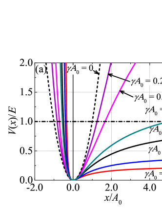
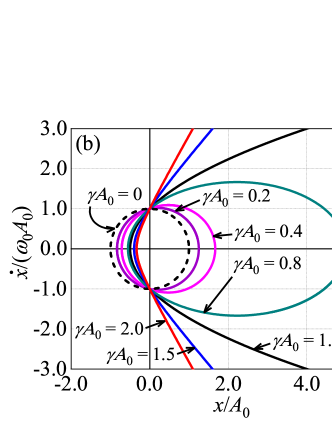
Figure 1: (a) Potentials $V(x)=\frac{1}{2}m(x)\omega_{0}^{2}x^{2}$ for the oscillator with PDM given by Eq. (6) and (b) phase portraits $(x,\dot{x})$ for deformation parameters: $\gamma A_{0}$ = 0 (usual case — circular trajectory); 0.2, 0.4, and 0.8 (elliptical trajectories); 1.0 (parabolic trajectory); and 1.5 and 2.0 (hyperbolic trajectories) [Eq. (11)]. For $\gamma A_{0}=0$, we recover the usual oscillator trajectory $\frac{x^{2}}{A_{0}^{2}}+\frac{\dot{x}^{2}}{A_{0}^{2}\omega_{0}^{2}}=1$. For $\gamma A_{0}=1$, the trajectory is the parabola $\frac{\dot{x}^{2}}{\omega_{0}^{2}A_{0}^{2}}=\frac{2x}{A_{0}}+1$.

Furthermore, the linear momentum evolves over time according to

$$p(t)=-m_{0}\omega_{0}A_{0}\sin\theta_{\gamma}(t)[1-\gamma A_{0}\cos\theta_{\gamma}(t)].$$ (15)

In general for systems with position-dependent kinetic energy terms, Bravo and Plyushchay showed that the classical Hamiltonians can be conveniently turned into systems with constant mass through the point canonical transformation [48]

$$\eta =\int^{x}\frac{\textrm{d}y}{\sqrt{g(y)}},$$ (16a)

$$\Pi =g(x)p,$$ (16b)

with $g(x)=\sqrt{m_{0}/m(x)}$, and $\eta$ being a deformed space and $\Pi$ named linear pseudomomentum, which satisfy the Poisson bracket $\{\eta,\Pi\}_{x,p}=1.$ In particular, for the mass function (6), from Eq. (16), we obtain[57, 60]

$$\eta =\frac{\ln(1+\gamma x)}{\gamma}\equiv x_{\gamma},$$ (17a)

$$\Pi =(1+\gamma x)p\equiv\Pi_{\gamma},$$ (17b)

and Hamiltonian (8) of a particle with PDM in the usual phase space $(x,p)$ is mapped into the Hamiltonian of a Morse oscillator in the deformed phase space $(x_{\gamma},\Pi_{\gamma})$,

$$\mathcal{K}(x_{\gamma},\Pi_{\gamma})=\frac{1}{2m_{0}}\Pi_{\gamma}^{2}+W_{\gamma}(e^{-\gamma x_{\gamma}}-1)^{2},$$ (18)

with the binding energy $W_{\gamma}=m_{0}\omega_{0}^{2}/2\gamma^{2}$ and the parameter of anamorticity $\gamma$. Therefore, the time evolution of the position $x_{\gamma}(t)$ and the linear momentum $\Pi_{\gamma}(t)$ is

$$x_{\gamma}(t) =-\frac{\ln(1-\gamma A_{0}\cos\theta_{\gamma}(t))}{\gamma},$$ (19a)

$$\Pi_{\gamma}(t) =-m_{0}\omega_{0}A_{0}\sin\theta_{\gamma}(t).$$ (19b)

Since $\gamma^{2}A_{0}^{2}=E/W_{\gamma}$, the particle presents closed path in the phase space $(x_{\gamma},p_{\gamma})$ for $E<W_{\gamma}$.

Figure 2 shows time evolution $x(t)$ and $p(t)$ as well as $x_{\gamma}(t)$ and $\Pi_{\gamma}(t)$ for $0\leq\gamma A_{0}<1$. The trajectories in both $(x,p)$ and $(x_{\gamma},\Pi_{\gamma})$ phase spaces are also shown. Figure 3 illustrates these same results, but now in the case $\gamma A_{0}>1$.

For $0<\gamma A_{0}<1$, the probability density for finding particle in the interval between $x$ and $x+\textrm{d}x$ is given by

$$\rho_{\textrm{classic}}(x)=\frac{1}{\pi\sqrt{A_{\gamma}^{2}-(x-\gamma A_{0}A_{\gamma})^{2}}},$$ (20)

so the first moments of position and linear momentum are

$$\overline{x} =\frac{\gamma A_{0}^{2}}{1-\gamma^{2}A_{0}^{2}},$$ (21a)

$$\overline{x^{2}} =\frac{A_{0}^{2}}{2}\frac{1+2\gamma^{2}A_{0}^{2}}{(1-\gamma^{2}A_{0}^{2})^{2}},$$ (21b)

$$\overline{p} =0,$$ (21c)

$$\overline{p^{2}} =\frac{1}{2}m_{0}^{2}\omega_{0}^{2}A_{0}^{2}\sqrt{1-\gamma^{2}A_{0}^{2}}.$$ (21d)

Similarly, the first moments of the linear pseudomomentum are

$$\overline{\,\Pi_{\gamma}} =0,$$ (22a)

$$\overline{\Pi_{\gamma}^{2}} =m_{0}^{2}\omega_{0}^{2}A_{0}^{2}\left(1-\frac{1-\sqrt{1-\gamma^{2}A_{0}^{2}}}{\gamma^{2}A_{0}^{2}}\right).$$ (22b)

It is straightforward to check that the mean value of the mass function is $\overline{m(x)}=m_{0}\sqrt{1-E/W_{\gamma}}$. The mean values of the kinetic and potential energies satisfy the curious relation $\overline{T(x)}=\overline{V(x)}\,\overline{m(x)}/m_{0},$ with $\overline{T(x)}\geq\overline{V(x)}$ since for closed path, we have $E\leq W_{\gamma}$. The standard virial theorem ($\overline{T}=\overline{V}$) is only valid for $\gamma=0$ ($W_{\gamma}\rightarrow\infty$).

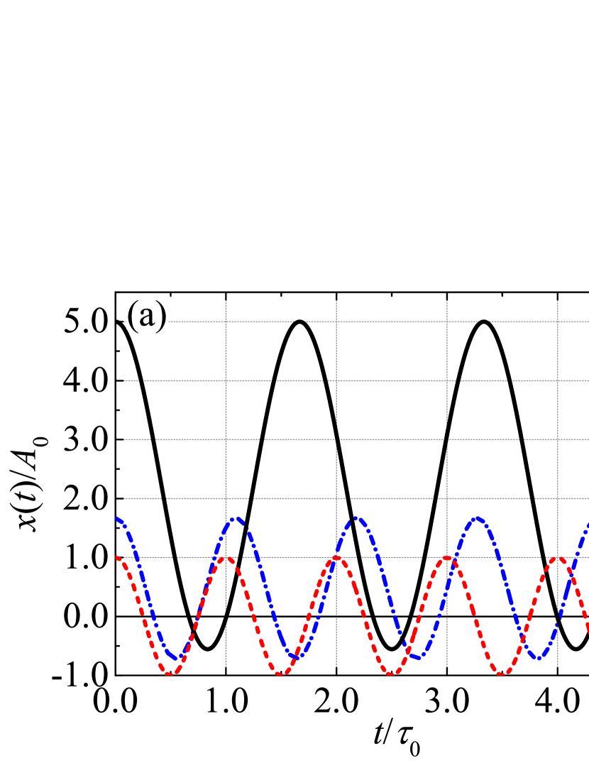
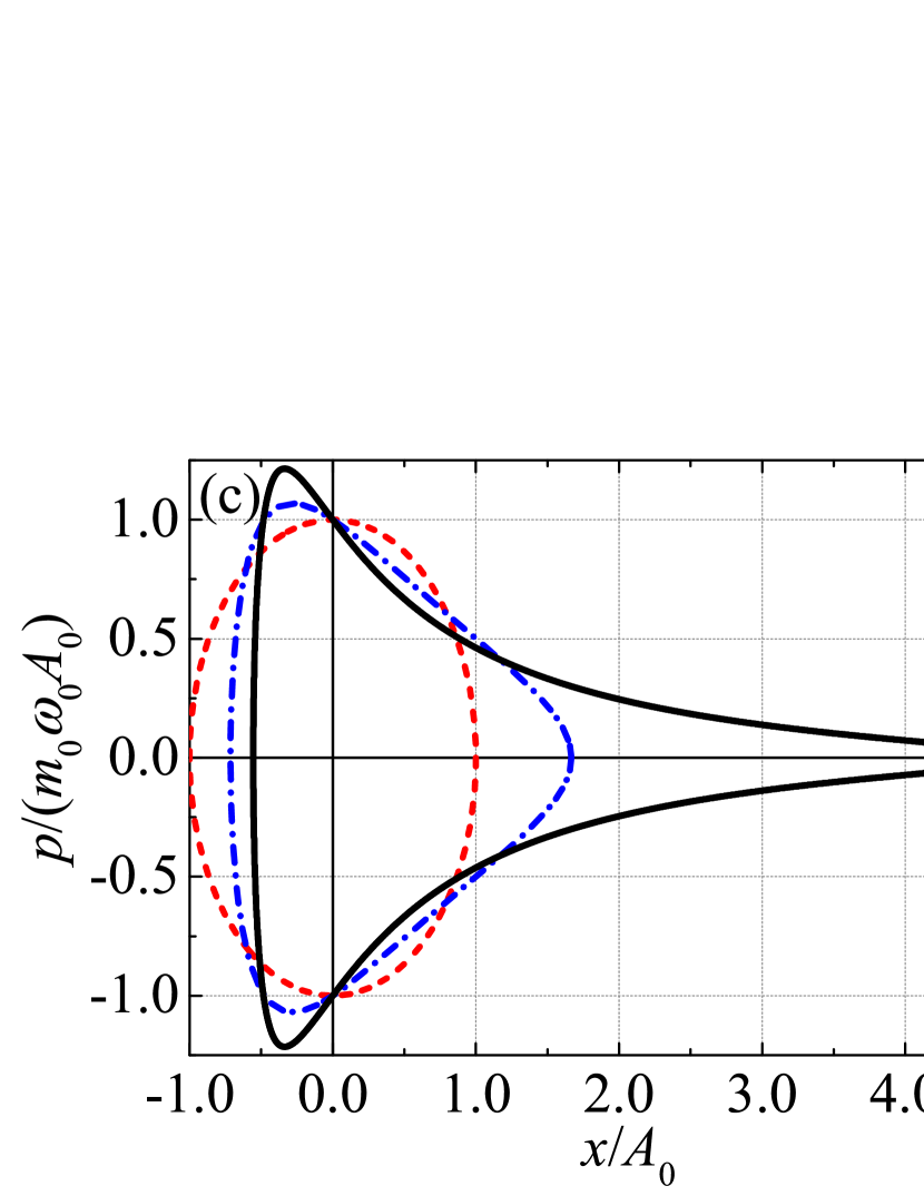
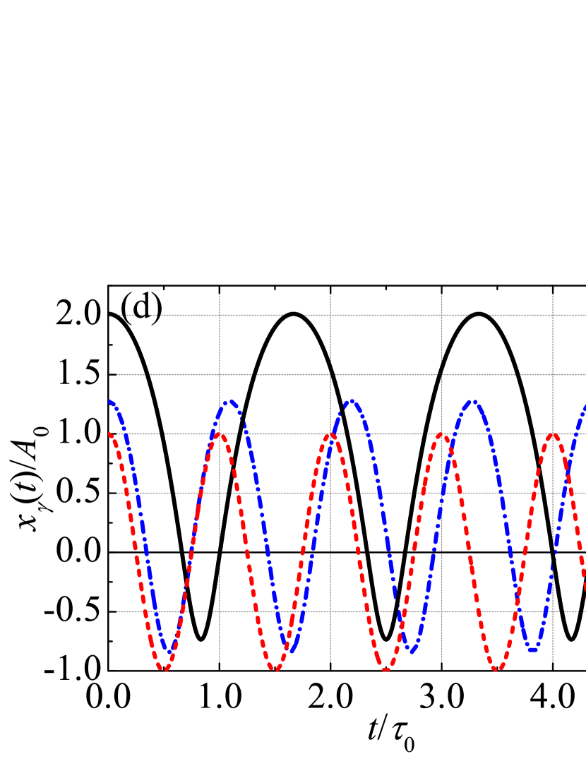
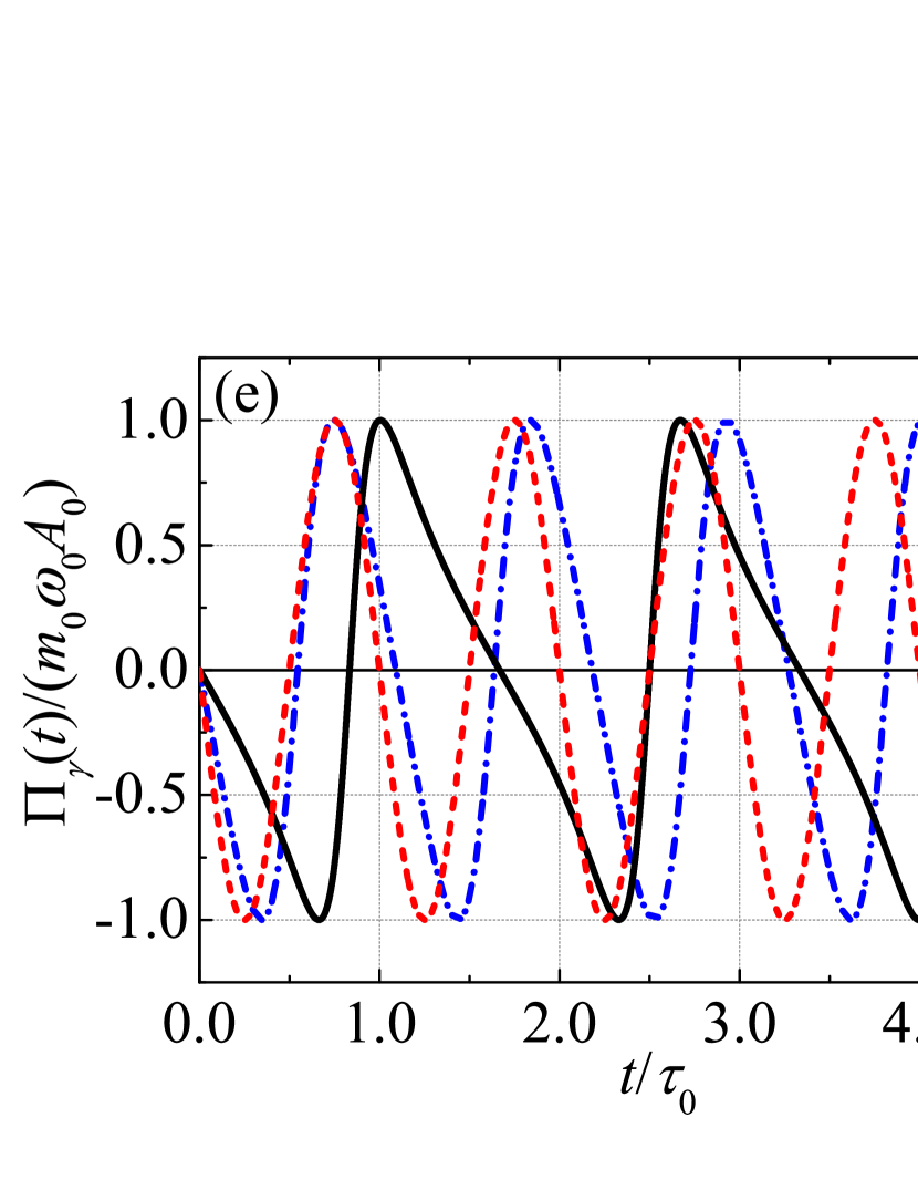
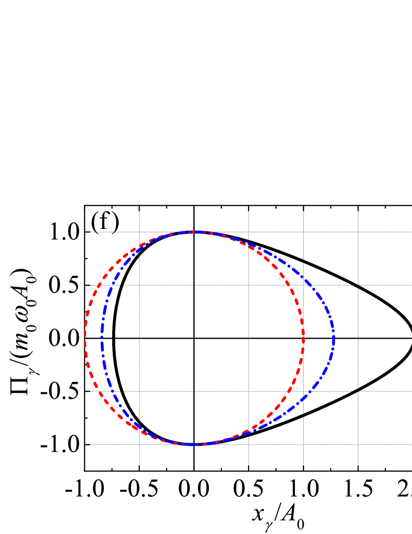
Figure 2: Deformed oscillator dynamics with $m(x)$ given by Eq. (6) and potential $V(x)=\frac{1}{2}m(x)\omega_{0}^{2}x^{2}$. Upper line: undeformed canonical coordinate representation — time evolution of (a) the position $x(t)$ and (b) the linear momentum $p(t)$ and (c) paths in phase space $(x,p)$. Bottom line: deformed canonical coordinate representation — time evolution of (d) the deformed position $x_{\gamma}(t)$ and (e) the linear pseudomomentum $\Pi_{\gamma}(t)$ and (f) paths in phase space $(x_{\gamma},\Pi_{\gamma})$. The deformation parameter in graphics are $\gamma A_{0}$ = 0 (dashed red line), 0.2 (dashed–dotted blue line), and 0.4 (solid black line).

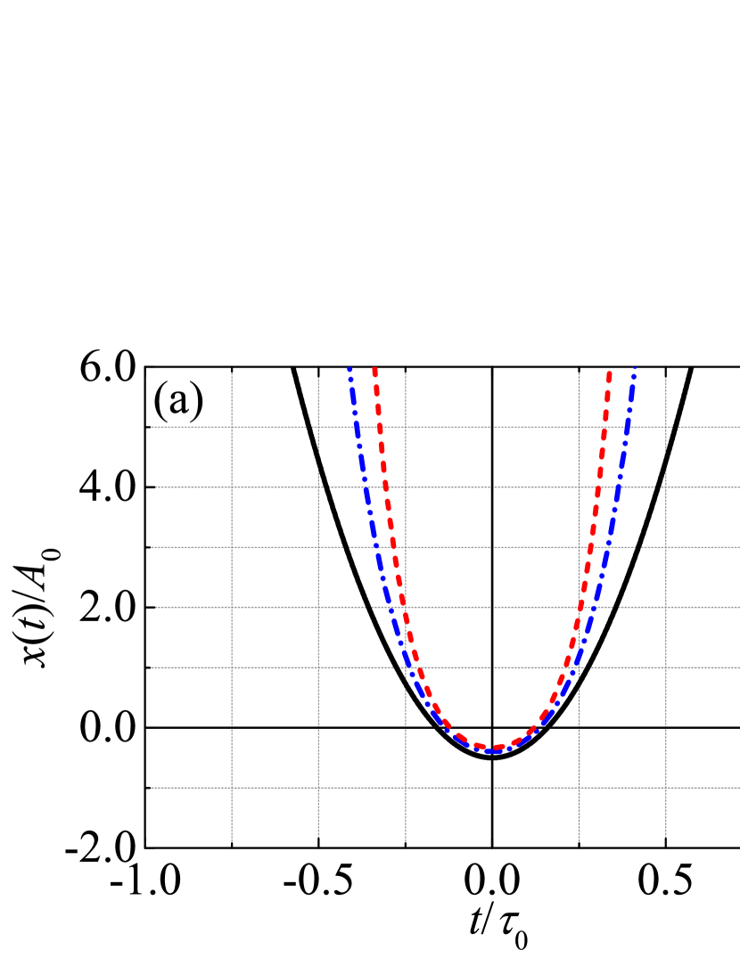
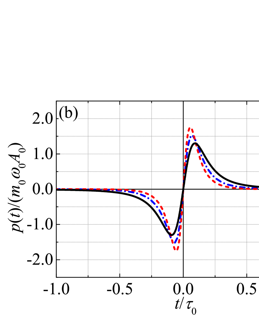
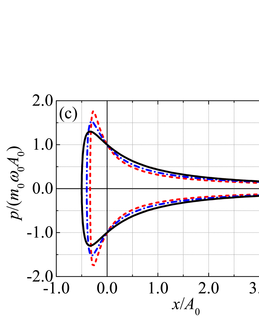
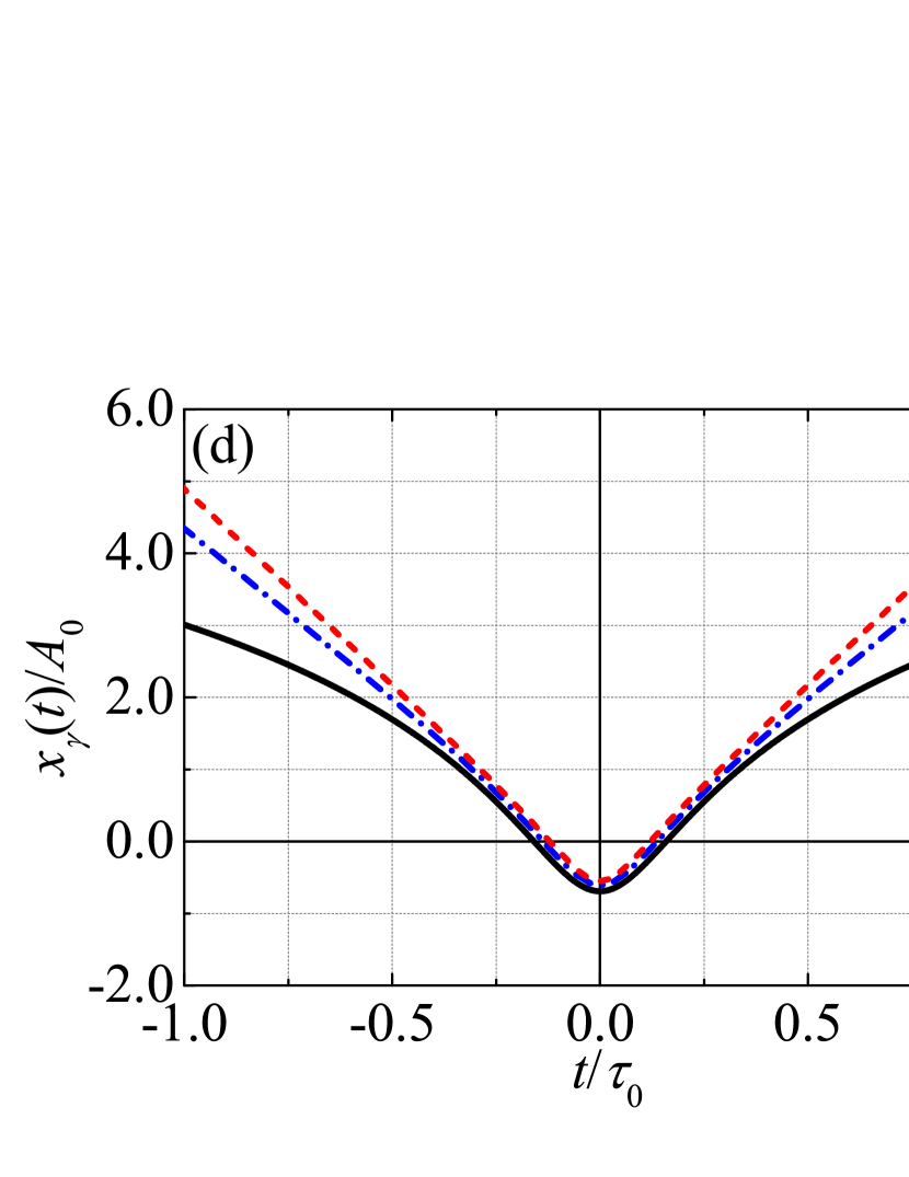
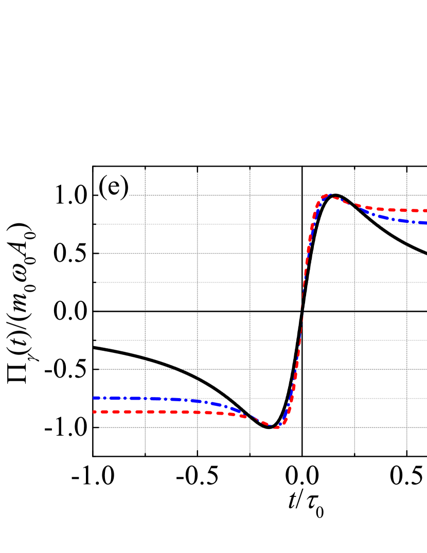
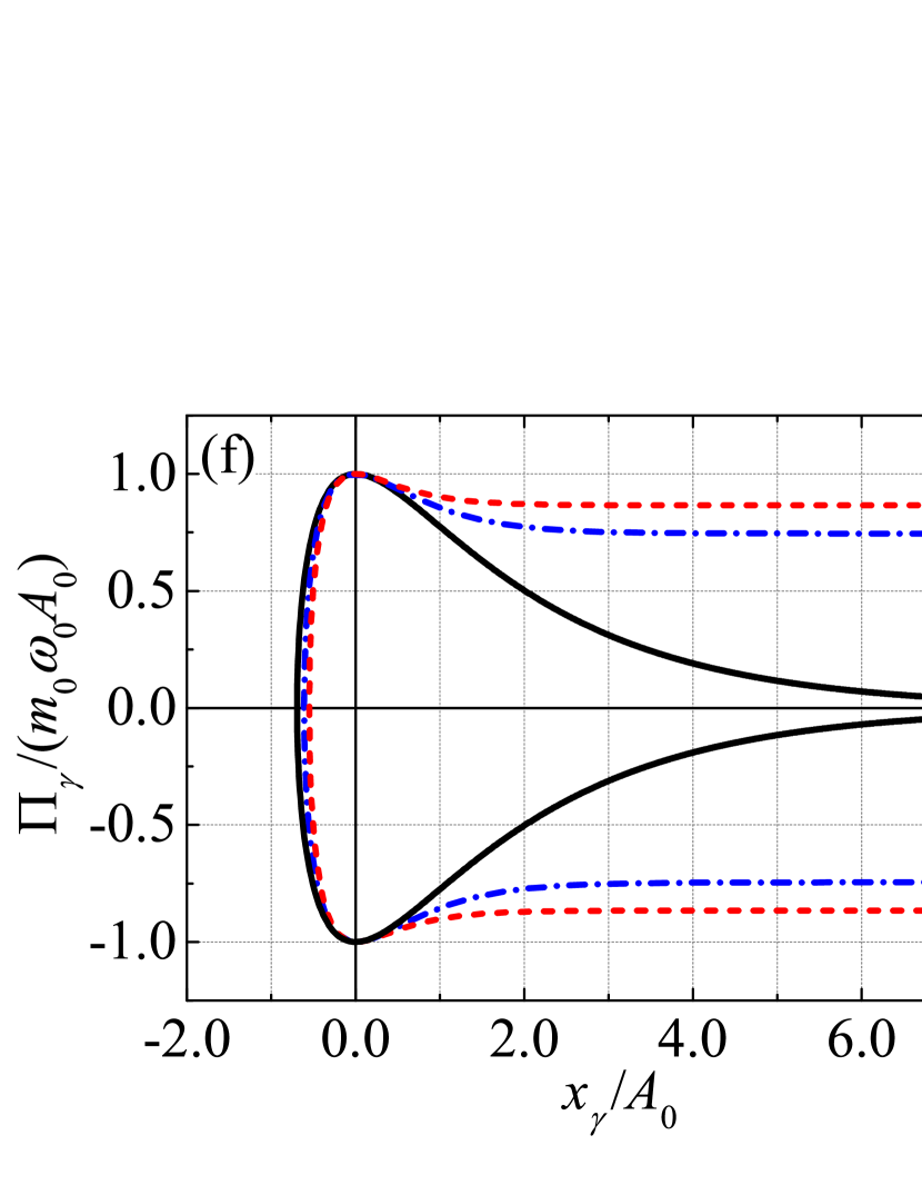
Figure 3: Phase space for open trajectories of the deformed oscillator dynamics with $m(x)$ given by Eq. (6) and potential $V(x)=\frac{1}{2}m(x)\omega_{0}^{2}x^{2}$. Upper line: undeformed canonical coordinates representation — time evolution of (a) the position $x(t)$ and (b) the linear momentum $p(t)$ and (c) paths in phase space $(x,p)$. Bottom line: deformed canonical coordinates representation — time evolution of (d) the deformed position $x_{\gamma}(t)$ and (e) the linear pseudomomentum $\Pi_{\gamma}(t)$ and (f) paths in phase space $(x_{\gamma},\Pi_{\gamma})$. The deformation parameter in graphics are $\gamma A_{0}$ = 1.0 (solid black line), 1.5 (dashed–dotted blue line), and 2.0 (dashed red line).

Alternatively, we can use the factorization method for obtaining the solution of the deformed oscillator. For this purpose, we consider the conjugate complex variables

$$\alpha_{\gamma}(x,p)=\sqrt{\frac{m_{0}\omega_{0}}{2\hbar}}\left[\frac{x}{1+\gamma x}+\frac{i}{m_{0}\omega_{0}}(1+\gamma x)p\right],$$ (23a)

$$\alpha_{\gamma}^{\ast}(x,p)=\sqrt{\frac{m_{0}\omega_{0}}{2\hbar}}\left[\frac{x}{1+\gamma x}-\frac{i}{m_{0}\omega_{0}}(1+\gamma x)p\right].$$ (23b)

Hence, the classical Hamiltonian (8) can be written as $\mathcal{H}=\hbar\omega_{0}\alpha_{\gamma}^{\ast}\alpha_{\gamma},$ with $\alpha_{\gamma}$, $\alpha_{\gamma}^{\ast}$ and $\mathcal{H}$ satisfying the Poisson brackets $\{\alpha_{\gamma},\alpha_{\gamma}^{\ast}\}=\frac{1}{i\hbar}\frac{1}{1+\gamma x}$, $\{\alpha_{\gamma},\mathcal{H}\}=-\frac{i\omega_{0}\alpha_{\gamma}}{1+\gamma x}$ and $\{\alpha_{\gamma}^{\ast},\mathcal{H}\}=\frac{i\omega_{0}\alpha_{\gamma}^{\ast}}{1+\gamma x}$, as well as the Jacobi identify $\{\{\alpha_{\gamma},\alpha_{\gamma}^{\ast}\},\mathcal{H}\}+\{\{\mathcal{H},\alpha_{\gamma}\},\alpha_{\gamma}^{\ast}\}+\{\{\alpha_{\gamma}^{\ast},\mathcal{H}\},\alpha_{\gamma}\}=0.$ In terms of dynamic variables $\alpha_{\gamma}(x,p)$ and $\alpha_{\gamma}^{\ast}(x,p)$, the Poisson brackets assume the deformed algebraic structure

$$\{\alpha_{\gamma},\alpha_{\gamma}^{\ast}\}=\frac{1}{i\hbar}\left[1-\frac{\gamma\sigma_{0}}{\sqrt{2}}\left(\alpha^{\ast}_{\gamma}+\alpha_{\gamma}\right)\right],$$ (24a)

$$\{\alpha_{\gamma},\mathcal{H}\}=-i\omega_{0}\alpha_{\gamma}\left[1-\frac{\gamma\sigma_{0}}{\sqrt{2}}\left(\alpha^{\ast}_{\gamma}+\alpha_{\gamma}\right)\right],$$ (24b)

$$\{\alpha_{\gamma}^{\ast},\mathcal{H}\}=i\omega_{0}\alpha_{\gamma}^{\ast}\left[1-\frac{\gamma\sigma_{0}}{\sqrt{2}}\left(\alpha^{\ast}_{\gamma}+\alpha_{\gamma}\right)\right].$$ (24c)

Thus, the dynamical variables $\alpha_{\gamma}$, $\alpha_{\gamma}^{\ast}$ and $\mathcal{H}$ lead to a deformed algebraic structure $\{\alpha_{\gamma},\alpha_{\gamma}^{\ast}\}=\mathcal{G}_{\gamma}(\alpha_{\gamma},\alpha_{\gamma}^{\ast})$, $\{\mathcal{H},\alpha_{\gamma}\}=i\omega_{0}\mathcal{G}_{\gamma}(\alpha_{\gamma},\alpha_{\gamma}^{\ast})\alpha_{\gamma}$ and $\{\mathcal{H},\alpha_{\gamma}^{\ast}\}=-i\omega_{0}\mathcal{G}_{\gamma}(\alpha_{\gamma},\alpha_{\gamma}^{\ast})$ with deformation established by the function $\mathcal{G}_{\gamma}(\alpha_{\gamma},\alpha_{\gamma}^{\ast})=1-\frac{\gamma\sigma_{0}}{\sqrt{2}}(\alpha_{\gamma}^{\ast}+\alpha_{\gamma})$. The standard case is recovered in the limit $\gamma\rightarrow 0$: $\lim_{\gamma\rightarrow 0}i\hbar\{\alpha_{\gamma},\alpha_{\gamma}^{\ast}\}=1$, $\lim_{\gamma\rightarrow 0}\{\mathcal{H},\alpha_{\gamma}\}=i\omega_{0}\alpha_{0}$, and $\lim_{\gamma\rightarrow 0}\{\mathcal{H},\alpha_{\gamma}^{\ast}\}=-i\omega_{0}\alpha_{0}^{\ast}$.

Of course, we have that the position, the linear momentum, and the linear pseudomomentum are, respectively,

$$x(t) =\frac{\sqrt{2}\sigma_{0}\textrm{Re}[\alpha_{\gamma}(t)]}{1-\sqrt{2}\sigma_{0}\gamma\textrm{Re}[\alpha_{\gamma}(t)]}$$ (25a)

$$p(t) =\sqrt{2}\frac{\hbar}{\sigma_{0}}\textrm{Im}[\alpha_{\gamma}(t)]\left\{1-\sqrt{2}\gamma\sigma_{0}\textrm{Re}[\alpha_{\gamma}(t)]\right\},$$ (25b)

$$\Pi_{\gamma}(t) =\sqrt{2}\frac{\hbar}{\sigma_{0}}\textrm{Im}[\alpha_{\gamma}(t)]$$ (25c)

with $\sigma_{0}=\sqrt{\frac{\hbar}{m_{0}\omega_{0}}}$ being a characteristic length of the usual oscillator ($\gamma=0$) and $\alpha_{\gamma}(t)=|\alpha_{\gamma}|e^{-i\theta_{\gamma}(t)}$. The complex number $\alpha_{\gamma}$ characterizes the state of the deformed harmonic oscillator.

To end this section, it is important to mention that the mass function $m(x)$ given by Eq. (6), and consequently the canonical transformation (17), are classical analog of the deformed space and linear momentum operators that emerge from the displacement operator method introduced by Costa Filho et al. [56, 57, 58, 59, 60, 61, 62, 63] to describe quantum systems with effective mass dependent on position, and thus, a Morse oscillator in the deformed space $x_{\gamma}=\gamma^{-1}\ln(1+\gamma x)$. According to Ref. 48, other different choices of the mass function and potential term can also lead to a Morse potential in a deformed space $\eta$. For example, consider a family classical Hamiltonians written in the form $\mathcal{H}_{\chi}(x,p)=\frac{p^{2}}{2\mathcal{M}(x)}+\mathcal{V}(x),$ with $\mathcal{V}(x)=\frac{1}{2}m_{0}\omega_{0}^{2}[\chi(x)]^{2}$ being a quadratic potential of the function $\chi(x)$ and $\mathcal{M}(x)$ being a generic mass function. Hence, the classical Hamiltonians $\mathcal{H}_{\chi}(x,p)$ are mapped into the Morse oscillator in the deformed phase space with constant mass $m_{0}$ and potential term $U_{\textrm{Morse}}(\eta)=\frac{m_{0}\omega_{0}^{2}}{2\gamma^{2}}(e^{-\gamma\eta}-1)^{2},$ since

$$\eta(x) =-\frac{1}{\gamma}\ln[1\mp\gamma\chi(x)],$$ (26a)

$$\mathcal{M}(x) =m_{0}\left[\frac{\chi^{\prime}(x)}{1\mp\gamma\chi(x)}\right]^{2}.$$ (26b)

The upper signal is equivalent to the lower one in Eq. (26) through the transformation $(\gamma,\chi,\eta)\rightarrow(-\gamma,-\chi,-\eta)$, which does not change the potential $\mathcal{V}(x)$ in the usual phase space $(x,p)$. Table 1 presents some different choices for the mass functions $\mathcal{M}(x)$ and the potential terms $\mathcal{V}(x)$ that lead to the Morse oscillator in deformed space. Hamiltonians $\mathcal{H}_{a}$ and $\mathcal{H}_{b}$ have the same mass function (unless replacement $\gamma\rightarrow-\gamma$) but different potentials $\mathcal{V}(x)$: asymmetric for $\mathcal{H}_{a}$ and symmetric for $\mathcal{H}_{b}$. The Hamiltonian $\mathcal{H}_{b}$ has been investigated in Refs. 60, 57. Hence, we choose to develop factorization methods, coherent states, and other topics in quantum mechanics on the asymmetric system $\mathcal{H}_{a}$, which has not yet been discussed in the literature. The other systems can be found in Ref. 64.

In addition, according Ref. 48, systems with PDM can be obtained from a particle with position-independent mass in Euclidean and Minkowski spaces. The Lagrangian family $\mathcal{L}=\frac{1}{2}\mathcal{M}(x)\dot{x}^{2}-\mathcal{V}(x)$ for classical systems shown in table 1 can be obtained by reduction from a particle in two-dimensional hyperbolic space $(X,Y)=(\sinh[\eta(x)/l_{0}],\cosh[\eta(x)/l_{0}])$ [with $\eta(x)$ depending on the mass function $\mathcal{M}(x)$ for each case]. The corresponding Lagrangian becomes $\mathcal{L}=\frac{m_{0}l_{0}^{2}}{2}(\dot{X}^{2}-\dot{Y}^{2})-U(Y)$, with $l_{0}$ being a characteristic length ($X$ and $Y$ are dimensionless) and the potential term being a modified Morse potential $U(Y)=\frac{m_{0}\omega_{0}^{2}}{2\gamma^{2}}\left[e^{-\gamma l_{0}\cosh^{-1}(Y)}-1\right]^{2}$. The mass function in this approach is given by $\mathcal{M}(x)=\frac{m_{0}l_{0}^{2}}{1+X^{2}}\left(\frac{\textrm{d}X}{\textrm{d}x}\right)^{2}$. Similarly, in a two-dimensional Euclidean space $(X,Y)=(\sin[\eta(x)/l_{0}],\cos[\eta(x)/l_{0}])$, the systems in table 1 lead to a Lagrangian $\mathcal{L}=\frac{m_{0}l_{0}^{2}}{2}(\dot{X}^{2}+\dot{Y}^{2})-U(Y)$, with modified Morse potential $U(Y)=\frac{m_{0}\omega_{0}^{2}}{2\gamma^{2}}\left[e^{-\gamma l_{0}\cos^{-1}(Y)}-1\right]^{2}$. The mass function is now given by $\mathcal{M}(x)=\frac{m_{0}l_{0}^{2}}{1-X^{2}}\left(\frac{\textrm{d}X}{\textrm{d}x}\right)^{2}$.

Table 1: Family of classical Hamiltonians $\mathcal{H}_{\chi}(x,p)=\frac{p^{2}}{2\mathcal{M}(x)}+\frac{1}{2}m_{0}\omega_{0}^{2}[\chi(x)]^{2}$ mapped into Morse oscillator $\mathcal{K}_{\textrm{Morse}}(\eta,\Pi)=\frac{1}{2m_{0}}\Pi^{2}+\frac{m_{0}\omega_{0}^{2}}{2\gamma^{2}}(e^{-\gamma\eta}-1)^{2}$ by means of the canonical transformation (16), with $\chi(x)$ and $\mathcal{M}(x)$ given by Eqs. (26). The deformation parameter $\gamma$ has dimension inverse length.

Case	$\chi(x)$	$\mathcal{M}(x)$	$\mathcal{V}(x)$	$(x_{1},x_{2})$	$\eta(x)$
$\mathcal{H}_{a}$	$\frac{x}{1+\gamma x}$	$\frac{m_{0}}{(1+\gamma x)^{2}}$	$\frac{m_{0}\omega_{0}^{2}x^{2}}{2(1+\gamma x)^{2}}$	$(-\frac{1}{\gamma},+\infty)$	$\frac{1}{\gamma}\ln(1+\gamma x)$
$\mathcal{H}_{b}$	$x$	$\frac{m_{0}}{(1-\gamma x)^{2}}$	$\frac{1}{2}m_{0}\omega_{0}^{2}x^{2}$	$(-\infty,\frac{1}{\gamma})$	$-\frac{1}{\gamma}\ln(1-\gamma x)$
$\mathcal{H}_{c}$	$\frac{\sqrt{1+\gamma^{2}x^{2}}-1-\gamma x}{\gamma}$	$\frac{m_{0}}{1+\gamma^{2}x^{2}}$	$\frac{m_{0}\omega_{0}^{2}}{2\gamma^{2}}\left(\sqrt{1+\gamma^{2}x^{2}}-1-\gamma x\right)^{2}$	$(-\infty,+\infty)$	$\frac{1}{\gamma}\sinh^{-1}(\gamma x)$
$\mathcal{H}_{d}$	$\displaystyle\frac{1-e^{-\tan^{-1}(\gamma x)}}{\gamma}$	$\frac{m_{0}}{(1+\gamma^{2}x^{2})^{2}}$	$\displaystyle\frac{m_{0}\omega_{0}^{2}}{2\gamma^{2}}\left[e^{-\tan^{-1}(\gamma x)}-1\right]^{2}$	$(-\infty,+\infty)$	$\frac{1}{\gamma}\tan^{-1}(\gamma x)$
$\mathcal{H}_{e}$	$\displaystyle\frac{1-e^{-\tan^{-1}(\sinh(\gamma x))}}{\gamma}$	$m_{0}\,\textrm{sech}^{2}(\gamma x)$	$\displaystyle\frac{m_{0}\omega_{0}^{2}}{2\gamma^{2}}\left[e^{-\tan^{-1}(\sinh(\gamma x))}-1\right]^{2}$	$(-\infty,+\infty)$	$\frac{1}{\gamma}\tan^{-1}(\sinh(\gamma x))$
$\mathcal{H}_{f}$	$\displaystyle\frac{1-e^{-\sinh^{-1}(\tan(\gamma x))}}{\gamma}$	$m_{0}\,\textrm{sec}^{2}(\gamma x)$	$\displaystyle\frac{m_{0}\omega_{0}^{2}}{2\gamma^{2}}\left[e^{-\sinh^{-1}(\tan(\gamma x))}-1\right]^{2}$	$(-\frac{\pi}{2\gamma},\frac{\pi}{2\gamma})$	$\frac{1}{\gamma}\sinh^{-1}(\tan(\gamma x))$

III Deformed quantum oscillator with position-dependent mass

As a consequence of the non-commutative structure of the mass function $m(\hat{x})$ and the linear momentum $\hat{p}$, the quantization of systems with PDM leads to the problem of ordering ambiguity in the definition of the kinetic energy operator. A general form for a Hermitian kinetic energy operator of a particle with PDM in one-dimensional was introduced by von Roos [17]

$$\hat{T}(\hat{x},\hat{p})=\frac{1}{4}\left\{[m(\hat{x})]^{-\delta_{1}}\hat{p}[m(\hat{x})]^{-1+\delta_{1}+\delta_{2}}\hat{p}[m(\hat{x})]^{-\delta_{2}}+[m(\hat{x})]^{-\delta_{2}}\hat{p}[m(\hat{x})]^{-1+\delta_{1}+\delta_{2}}\hat{p}[m(\hat{x})]^{-\delta_{1}}\right\},$$ (27)

with $\delta_{1}$ and $\delta_{2}$ named ambiguity parameters. Several proposals for the kinetic energy operator are particular case of (27), such as, Ben Daniel and Duke ($\delta_{1}=\delta_{2}=0$),[18] Gora and Williams ($\delta_{1}=1$, $\delta_{2}=0$),[19] Zhu and Kroemer ($\delta_{1}=\delta_{2}=\frac{1}{2}$),[20] Li and Kuhn ($\delta_{1}=0,\delta_{2}=\frac{1}{2}$).[21] Morrow and Brownstein[22] investigated that the case $\delta_{1}=\delta_{2}$ obeys conditions of continuity of the wave function at the boundaries of a heterojunction in crystals. In particular, Mustafa and Mazharimousavi [23] showed that the case $\delta_{1}=\delta_{2}=\frac{1}{4}$ allows the mapping of a quantum Hamiltonian with PDM into another Hamiltonian with constant mass through a point canonical transformation, regardless of the potential $V(\hat{x})$ to which the particle is subjected. For classical Hamiltonians with kinetic terms including PDM, Bravo and Plyushchay[48] introduced a fictitious gauge transformation, which leads to a more general ordering that includes all these particular cases pointed out in Refs. 18, 19, 20, 21, 22, 23.

Considering the quantum Hamiltonian

$$\hat{H}(\hat{x},\hat{p})=\frac{1}{2}[m(\hat{x})]^{-\frac{1}{4}}\hat{p}[m(\hat{x})]^{-\frac{1}{2}}\hat{p}[m(\hat{x})]^{-\frac{1}{4}}+V(\hat{x}),$$ (28)

the time-independent Schrödinger equation $\hat{H}|\psi\rangle=E|\psi\rangle$ in the position representation $\{|\hat{x}\rangle\}$ is

$$\left(-\frac{\hbar^{2}}{2m_{0}}\sqrt[4]{\frac{m_{0}}{m(x)}}\frac{\textrm{d}}{\textrm{d}x}\sqrt{\frac{m_{0}}{m(x)}}\frac{\textrm{d}}{\textrm{d}x}\sqrt[4]{\frac{m_{0}}{m(x)}}+V(x)\right)\psi(x)=E\psi(x),$$ (29)

where $E$ is the eigenvalue corresponding to the eigenfunction $\psi(x)$ of $\hat{H}$.

Let the linear pseudomomentum introduced previously by Mustafa and Mazharimousavi be [23]

$$\hat{\Pi}\equiv\sqrt{g(\hat{x})}\,\hat{p}\,\sqrt{g(\hat{x})}=\frac{1}{2}(\hat{P}_{g}^{\dagger}+\hat{P}_{g})$$ (30)

with $g(\hat{x})=\sqrt{m_{0}/m(\hat{x})}$ being a spatial metric term and $\hat{P}_{g}\equiv g(\hat{x})\hat{p}$ being a non-Hermitian linear momentum. The linear pseudomomentum (30) has also been investigated recently by Plyushchay[65] from the anomaly-free prescription so that the structure is used to get quantization of particles in curved spaces. Hamiltonian (28) can be written in the simplified form $\hat{H}(\hat{x},\hat{p})=\frac{1}{2m_{0}}\hat{\Pi}^{2}(\hat{x},\hat{p})+V(\hat{x}).$ Note that the linear pseudomomentum $\hat{\Pi}$ is the physical quantity conserved for a free particle with PDM ($V(\hat{x})=0$). Moreover, $\hat{x}$ and $\hat{\Pi}$ satisfy the commutation relation $[\hat{x},\hat{\Pi}]=i\hbar g(\hat{x})$, so this algebraic structure results in a generalized uncertainty principle,

$$\Delta x\Delta\Pi\geq\frac{\hbar}{2}|\langle g(\hat{x})\rangle|.$$ (31)

Alternatively, we can rewrite Eq. (29) by means of the transformation $\varphi(x)=\sqrt{g(x)}\psi(x)$, such that

$$\left[-\frac{\hbar^{2}}{2m_{0}}\left(g(x)\frac{\textrm{d}}{\textrm{d}x}\right)^{2}+V(x)\right]\varphi(x)=E\varphi(x),$$ (32)

which is associated with the Hamiltonian operator $\hat{H}_{g}(\hat{x},\hat{P}_{g})=\frac{1}{2m_{0}}\hat{P}_{g}^{2}+V(\hat{x}).$ From deformed space $\hat{\eta}\equiv\int^{\hat{x}}[g(y)]^{-1}\textrm{d}y=\int^{\hat{x}}\sqrt{m(y)/m_{0}}\textrm{d}y$, we obtain the standard commutation relation $[\hat{\eta},\hat{\Pi}]=i\hbar\hat{1}$. Therefore, we have that $(\hat{x},\hat{p})\rightarrow(\hat{\eta},\hat{\Pi})$ constitutes a point canonical transformation that maps the Hamiltonian (28) with PDM into another Hamiltonian with constant mass $\hat{K}(\hat{\eta},\hat{\Pi})=\frac{1}{2m_{0}}\hat{\Pi}^{2}+U(\hat{\eta}),$ whose potential in the deformed space is $U(\hat{\eta})=V(\hat{x}(\hat{\eta}))$. The corresponding Schrödinger equation in the deformed space is denoted by $\hat{K}\phi(\eta)=E\phi(\eta)$, with $\phi(\eta)=\varphi(x(\eta))$ being the wave function in representation $\{|\hat{\eta}\rangle\}$.

For the mass function (6), the spatial metric term is $g(\hat{x})=\hat{1}+\gamma\hat{x}$, and the deformed space and linear pseudomomentum are given, respectively, by

$$\hat{x}_{\gamma} =\frac{\ln(1+\gamma\hat{x})}{\gamma},$$ (33a)

$$\hat{\Pi}_{\gamma} =(\hat{1}+\gamma\hat{x})^{1/2}\hat{p}(\hat{1}+\gamma\hat{x})^{1/2}=\frac{1}{2}(\hat{p}_{\gamma}^{\dagger}+\hat{p}_{\gamma}),$$ (33b)

with $\hat{p}_{\gamma}=-i\hbar D_{\gamma}$ and $D_{\gamma}\varphi(x)=(1+\gamma x)\frac{\textrm{d}\varphi(x)}{\textrm{d}x}$ being a deformed derivative [dual to $\mathcal{D}_{\gamma}x(t)=\frac{1}{1+\gamma x}\frac{\textrm{d}x}{\textrm{d}t}$ — see Ref. 60 for more details].

Considering the potential $V(x)=\frac{1}{2}m(x)\omega_{0}^{2}x^{2}$ with mass function (6), one can write Eq. (32) as a deformed Schrödinger equation for the problem of the asymmetric oscillator with PDM [56, 60]

$$-\frac{\hbar^{2}}{2m_{0}}D_{\gamma}^{2}\varphi(x)+\frac{m_{0}\omega_{0}^{2}x^{2}}{2(1+\gamma x)^{2}}\varphi(x)=E\varphi(x).$$ (34)

In the deformed space $x_{\gamma}$, Eq. (34) can be expressed in terms of the new field $\phi(x_{\gamma})=\varphi(x(x_{\gamma}))$, and it becomes the Schrödinger equation for the quantum Morse oscillator,[57, 60]

$$-\frac{\hbar^{2}}{2m_{0}}\frac{\textrm{d}^{2}{\phi}(x_{\gamma})}{\textrm{d}x_{\gamma}^{2}}+W_{\gamma}(e^{-\gamma x_{\gamma}}-1)^{2}\phi({x_{\gamma}})=E\phi({x_{\gamma}}).$$ (35)

The eigenfunctions of Eq. (35) are

$$\phi_{n}(x_{\gamma})=(-1)^{n}\mathcal{N}_{n}e^{-\frac{1}{2}\xi(x_{\gamma})}[\xi(x_{\gamma})]^{\frac{\nu_{n}}{2}}L_{n}^{(\nu_{n})}(\xi(x_{\gamma})),$$ (36)

where $\xi(x_{\gamma})=2se^{-\gamma x_{\gamma}},$ $s=\frac{1}{\gamma^{2}\sigma_{0}^{2}},$ $\nu_{n}=2s-2n-1>0,$ $\mathcal{N}_{n}^{2}=\nu_{n}\gamma\Gamma(n+1)/\Gamma(\nu_{n}+n+1),$ and $L_{n}^{(\nu)}(z)$ are the associated Laguerre polynomials. From the solutions of (35), we obtain the normalized eigenfunctions of the deformed oscillator,

$$\psi_{n}(x) =\frac{\varphi_{n}(x)}{\sqrt{1+\gamma x}}=(-1)^{n}\frac{\mathcal{N}_{n}}{\sqrt{2s}}e^{-\frac{\zeta(x)}{2}}[\zeta(x)]^{\frac{\nu_{n}+1}{2}}L_{n}^{(\nu_{n})}(\zeta(x))$$ (37)

for $x>-1/\gamma$ and $\psi_{n}(x)=0$ otherwise, where $\zeta(x)=\frac{2s}{1+\gamma x}$. The energy eigenvalues are

$$E_{n}({\gamma})=\hbar\omega_{0}\left(n+\frac{1}{2}\right)-\frac{\hbar^{2}\gamma^{2}}{2m_{0}}\left(n+\frac{1}{2}\right)^{2}.$$ (38)

Curiously, this energy spectrum is identical to the case of the quadratic potential $V_{0}(x)=\frac{1}{2}m_{0}\omega_{0}^{2}x^{2}$ previously studied in Ref. 61. From the condition $E_{n}<W_{\gamma}$, the number of bound states is restricted by the condition $0\leq n+\frac{1}{2}<\frac{m_{0}\omega_{0}}{\hbar\gamma^{2}}$ (i.e., $\nu_{n}>0$).

In particular, the eigenfunction for $n=0$ is

$$\psi_{0}(x)=\sqrt{\frac{\gamma}{2s\Gamma(2s-1)}}e^{-\frac{\zeta(x)}{2}}[\zeta(x)]^{s}.$$ (39)

The probability density $\rho_{0}(x)=|\psi_{0}(x)|^{2}$ behaves like a Gamma distribution,

$$\rho_{0}(x)=\frac{\gamma}{2s}\frac{1}{\Gamma(\lambda)}e^{-\zeta(x)}[\zeta(x)]^{\lambda+1},$$ (40)

with $\lambda=\frac{2}{\gamma^{2}\sigma_{0}^{2}}-1$ being the shape parameter. The ground state energy is $E_{0}({\gamma})=\frac{\hbar\omega_{0}}{2}-\frac{\hbar^{2}\gamma^{2}}{8m_{0}}.$

For $E>W_{\gamma}$, the eigenstates become unbound and the eigenfunctions are the non-normalized wavefunction

$$\psi(x)=\frac{e^{-\frac{\zeta(x)}{2}}}{\sqrt{2s}}[\zeta(x)]^{w+\frac{1}{2}}\left[C_{1}\,L_{s-1-w}^{(2w)}(\zeta(x))+C_{2}\,{{}_{1}}F_{1}\left(1+w-s;1+2w;\zeta(x)\right)\right]\!,$$ (41)

where ${}_{1}F_{1}(\,\cdot\,;\,\cdot\,;\,\cdot\,)$ represent the confluent hypergeometric functions of the first kind, $C_{1}$ and $C_{2}$ are constants, and $w^{2}=2m_{0}(E-W_{\gamma})/\hbar^{2}\gamma^{2}$. For the sake of simplicity, we will continue in this work discussing the properties of the bound states for the deformed oscillator.

In Fig. 4, we plot eigenfunctions $\psi_{n}(x)$ and density probabilities $\rho_{n}(x)=|\psi_{n}(x)|^{2}$ for the ground state and the first two excited states with different values of the deformation parameter $\gamma\sigma_{0}$. Figure 5 shows that for large quantum numbers, exemplified here with $n=20$, the mean quantum probability density $\rho_{n}(x)$ tends to approach the classical probability density $\rho_{\textrm{classic}}(x)$ [Eq. (20)] with $A_{\gamma,n}^{2}=2E_{n}(\gamma)/m_{0}\omega_{0}^{2}$ in place of $A_{0}^{2}$.

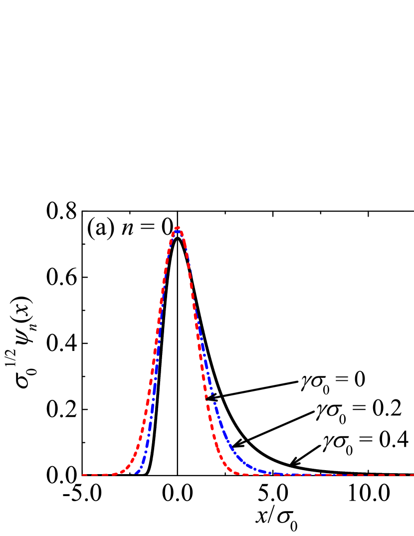
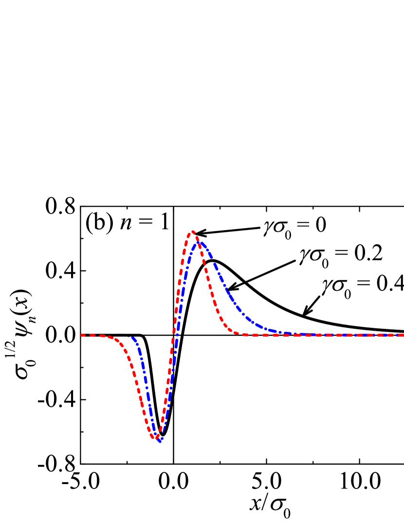
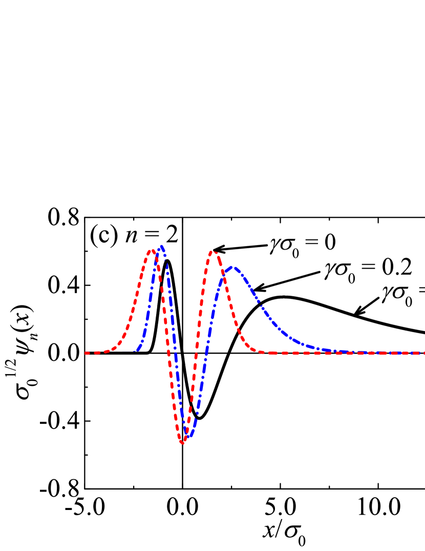
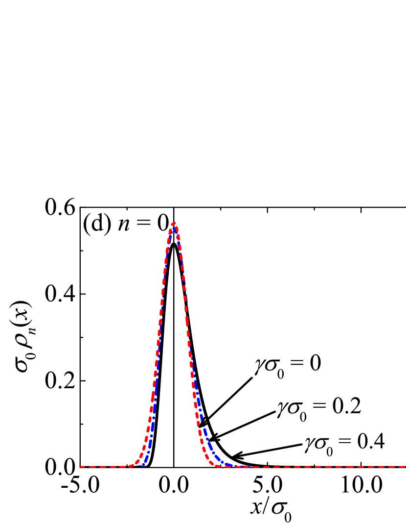
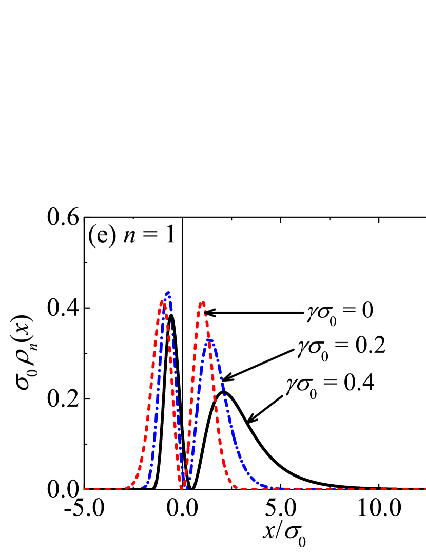
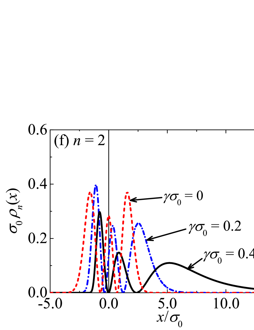
Figure 4: Wave functions $\psi_{n}(x)$ (upper line) and probability densities $\rho_{n}(x)$ (bottom line) for deformed oscillator with PDM and values of $\gamma\sigma_{0}=0$ (standard case for comparison, dashed red line), $0.2$ (dashed–dotted blue line), and $0.4$ (solid black line). [(a) and (d)] $n=0$ (ground state), [(b) and (e)] $n=1$ (first excited state), and [(c) and (f)] $n=2$ (second excited state).

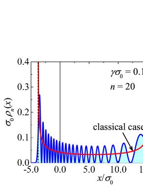
Figure 5: Probability density for a deformed oscillator with PDM given by Eq. (6) and potential $V(x)=\frac{1}{2}m(x)\omega_{0}^{2}x^{2}$ with $\gamma\sigma_{0}=0.1$ and $n=20$. The classical case [Eq. (20)] (with $A_{\gamma,n}^{2}=2E_{n}(\gamma)/m_{0}\omega_{0}^{2}$ replaced by $A_{0}^{2}$) is shown for comparison. Dotted vertical lines correspond to $x_{\textrm{min}}=-A_{\gamma,n}/(1+\gamma A_{\gamma,n})$ and $x_{\textrm{max}}=A_{\gamma,n}/(1-\gamma A_{\gamma,n})$.

We obtain that the expected values of the potential and kinetic energies are given respectively by

$$\langle\hat{V}\rangle =\frac{\hbar\omega_{0}}{2}\left(n+\frac{1}{2}\right),$$ (42a)

$$\langle\hat{T}\rangle =\frac{\hbar\omega_{0}}{2}\left(n+\frac{1}{2}\right)\left[1-\gamma^{2}\sigma_{0}^{2}\left(n+\frac{1}{2}\right)\right].$$ (42b)

Figure 6 illustrates the potential $V(x)$ (in terms of the standard ground energy $\varepsilon_{0}=\frac{1}{2}\hbar\omega_{0}$) and the energy levels (38) of the bound states. Together, a comparison between $E_{n}$, $\langle\hat{T}\rangle$ and $\langle\hat{V}\rangle$ is illustrated.

Similarly, we calculate that the expected value of mass operator $m(\hat{x})$ is $\langle m(\hat{x})\rangle=m_{0}\left[1-\gamma^{2}\sigma_{0}^{2}\left(n+\frac{1}{2}\right)\right],$ in which it leads to the relationship $\langle\hat{T}\rangle={\langle\hat{V}\rangle\langle m(\hat{x})\rangle}/{m_{0}}$. Note that $\langle\hat{T}\rangle\geq\langle\hat{V}\rangle$, and the equality is satisfied only for the usual case ($\gamma=0$, i.e., $\langle m(\hat{x})\rangle={m_{0}}$).

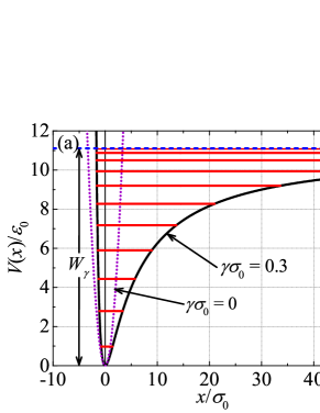
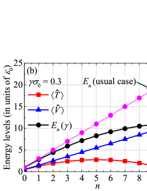
Figure 6: (a) Energy levels of the bound states for the oscillator with PDM $m(x)$ [Eq. (6)] and potential $V(x)=\frac{1}{2}m(x)\omega_{0}^{2}x^{2}$. The deformation parameter is $\gamma\sigma_{0}=0.3$, with $\varepsilon_{0}=\frac{1}{2}\hbar\omega_{0}$. (b) Expected values $\langle\hat{T}\rangle$, $\langle\hat{V}\rangle$, and $E_{n}$ as a function of the quantum number $n$ (the usual case $\gamma\sigma_{0}=0$ is shown for comparison).

After some careful calculations, we obtain that the expected values $\langle\hat{x}\rangle$, $\langle\hat{x}^{2}\rangle$, $\langle\hat{p}\rangle$ and $\langle\hat{p}^{2}\rangle$ for the $n$th eigenstate are given by

$$\langle\hat{x}\rangle =\frac{1}{\gamma}\left\{\frac{1}{\left[1-\gamma^{2}\sigma_{0}^{2}\left(n+\frac{1}{2}\right)\right]^{2}-\frac{\gamma^{2}\sigma_{0}^{2}}{4}}-1\right\},$$ (43a)

$$\langle\hat{x}^{2}\rangle =\frac{1}{\gamma^{2}}\frac{1+\gamma^{2}\sigma_{0}^{2}\left(n+\frac{1}{2}\right)-\frac{1}{2}\gamma^{4}\sigma_{0}^{4}n(n+1)}{\left\{\left[1-\gamma^{2}\sigma_{0}^{2}\left(n+\frac{1}{2}\right)\right]^{2}-\frac{\gamma^{4}\sigma_{0}^{4}}{4}\right\}\left\{\left[1-\gamma^{2}\sigma_{0}^{2}\left(n+\frac{1}{2}\right)\right]^{2}-\gamma^{4}\sigma_{0}^{4}\right\}}$$

$$\quad-\frac{2}{\gamma^{2}}\frac{1}{\left[1-\gamma^{2}\sigma_{0}^{2}\left(n+\frac{1}{2}\right)\right]^{2}-\frac{\gamma^{4}\sigma_{0}^{4}}{4}}+\frac{1}{\gamma^{2}},$$ (43b)

$$\langle\hat{p}\rangle =0,$$ (43c)

$$\langle\hat{p}^{2}\rangle =\frac{\hbar^{2}}{\sigma_{0}^{2}}\left[\left(n+\frac{1}{2}\right)-\frac{\gamma^{2}\sigma_{0}^{2}}{2}(n^{2}+n-1)\right]\left[1-\gamma^{2}\sigma_{0}^{2}\left(n+\frac{1}{2}\right)\right].$$ (43d)

Similarly, it is straightforward to verify that the expected values of the linear pseudomomentum are

$$\langle\hat{\Pi}_{\gamma}\rangle =0,$$ (44a)

$$\langle\hat{\Pi}_{\gamma}^{2}\rangle =\frac{\hbar^{2}}{\sigma_{0}^{2}}\left(n+\frac{1}{2}\right)\left[1-\gamma^{2}\sigma_{0}^{2}\left(n+\frac{1}{2}\right)\right].$$ (44b)

The expected values $\langle\hat{p}^{2}\rangle$ and $\langle\hat{\Pi}_{\gamma}^{2}\rangle$ different for $\gamma\neq 0$. We can clearly see that in the limit $\gamma=0$ the usual cases are recovered: $\lim_{\gamma\rightarrow 0}\langle\hat{x}\rangle=0$, $\lim_{\gamma\rightarrow 0}\langle\hat{x}^{2}\rangle=\sigma_{0}^{2}\left(n+\frac{1}{2}\right)$ and $\lim_{\gamma\rightarrow 0}\langle\hat{p}^{2}\rangle=\lim_{\gamma\rightarrow 0}\langle\hat{\Pi}_{\gamma}^{2}\rangle=\frac{\hbar^{2}}{\sigma_{0}^{2}}\left(n+\frac{1}{2}\right)$.

Since $A_{\gamma,n}^{2}=2\sigma_{0}^{2}E_{n}({\gamma})/\hbar\omega_{0}$, according to the principle of correspondence, in the limit of large quantum numbers (or $\hbar\rightarrow 0$), we have $E_{n}\gg\hbar\omega_{0}$, and consequently, Eqs. (43) can be written as

$$\langle\hat{x}\rangle =\frac{\gamma A_{\gamma,n}^{2}}{1-\gamma^{2}A_{\gamma,n}^{2}},$$ (45a)

$$\langle\hat{x}^{2}\rangle =\frac{A_{\gamma,n}^{2}}{2}\frac{1+2\gamma^{2}A_{\gamma,n}^{2}}{(1-\gamma^{2}A_{\gamma,n}^{2})^{2}},$$ (45b)

$$\langle\hat{p}^{2}\rangle =\frac{1}{2}m_{0}^{2}\omega_{0}^{2}A_{\gamma,n}^{2}\sqrt{1-\gamma^{2}A_{\gamma,n}^{2}},$$ (45c)

which coincide with the corresponding mean values of the classic oscillator [Eq. (21)].

In Fig. 7, we plot the square of the uncertainties of $x$ and $p$, $(\Delta x)^{2}$ and $(\Delta p)^{2}$, along with the uncertainty relation $\Delta x\Delta p$ for states $n=0$, $1$ and $2$. As the dimensionless parameter $|\gamma\sigma_{0}|$ approaches 1, the position uncertainty increases and the linear momentum one decreases (except for state $n=0$ which has a peculiar behavior), but as expected, the standard uncertainty relation $\Delta x\Delta p\geq\frac{\hbar}{2}$ is kept. In addition, the uncertainty product is symmetric around $\gamma\sigma_{0}=0$ and grows with the quantum number $n$. On the other hand, for the mass function (6), we have the spatial metric term $g(\hat{x})=1+\gamma\hat{x}$ so that the observables $\hat{x}$ and $\hat{\Pi}_{\gamma}$ satisfy the generalized uncertainty principle $\Delta x\Delta\Pi_{\gamma}\geq\frac{\hbar}{2}(1+\gamma\langle\hat{x}\rangle)$, as shown in the figure 7(d). Despite the different expressions for expected values of $\langle\hat{p}^{2}\rangle$ and $\langle\hat{\Pi}_{\gamma}^{2}\rangle$, the products of uncertainty are quite similar $\Delta x\Delta p$ and $\Delta x\Delta\Pi_{\gamma}$.

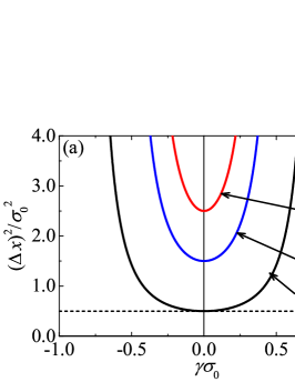
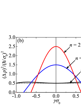
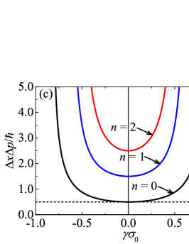
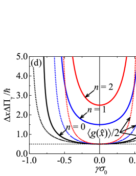
Figure 7: Mean square deviation of (a) position $x$ and (b) linear momentum $p$ and products (c) $\Delta x\Delta p$ and (d) $\Delta x\Delta\Pi_{\gamma}$ of the deformed oscillator as a function of the dimensionless parameter $\gamma\sigma_{0}$ for the states $n=0$, $1$ and $2$.

IV Coherent states for deformed oscillator

IV.1 Factorization method for quantum deformed oscillator

For the potential $V(\hat{x})=\frac{1}{2}m(x)\omega_{0}^{2}\hat{x}^{2},$ the Hamiltonian operator (28) can be factorized as

$$\hat{H}=\hbar\omega_{0}\hat{a}_{\gamma}^{\dagger}\hat{a}_{\gamma}+E_{0}({\gamma}),$$ (46)

with the annihilation and the creation operators given by

$$\hat{a}_{\gamma} =\sqrt{\frac{m_{0}\omega_{0}}{2\hbar}}\left[\frac{\hat{x}}{\hat{1}+\gamma\hat{x}}+\frac{i}{m_{0}\omega_{0}}(\hat{1}+\gamma\hat{x})\hat{p}\right]$$

$$=\sqrt{\frac{m_{0}\omega_{0}}{2\hbar}}\left[\hat{\Phi}_{\gamma}(\hat{x})+\frac{i}{m_{0}\omega_{0}}\hat{\Pi}_{\gamma}(\hat{x},\hat{p})\right]$$ (47a)

and

$$\hat{a}_{\gamma}^{\dagger} =\sqrt{\frac{m_{0}\omega_{0}}{2\hbar}}\left[\frac{\hat{x}}{\hat{1}+\gamma\hat{x}}-\frac{i}{m_{0}\omega_{0}}\hat{p}(\hat{1}+\gamma\hat{x})\right]$$

$$=\sqrt{\frac{m_{0}\omega_{0}}{2\hbar}}\left[\hat{\Phi}_{\gamma}(\hat{x})-\frac{i}{m_{0}\omega_{0}}\hat{\Pi}_{\gamma}(\hat{x},\hat{p})\right],$$ (47b)

where $\hat{\Phi}_{\gamma}(\hat{x})=\frac{\hat{x}}{\hat{1}+\gamma\hat{x}}-\frac{\hbar\gamma}{2m_{0}\omega_{0}}$ corresponds to superpotential[52] and satisfies along linear pseudomomentum $\hat{\Pi}_{\gamma}$ the relation $[\hat{\Phi}_{\gamma},\hat{\Pi}_{\gamma}]=\frac{i\hbar}{\sqrt{m(\hat{x})/m_{0}}}\frac{\textrm{d}\Phi_{\gamma}(\hat{x})}{\textrm{d}\hat{x}}=\frac{i\hbar}{1+\gamma\hat{x}}$. It is easy to verify that $\hat{a}_{\gamma}\psi_{0}(x)=0$, i.e., the ground state [Eq. (39)] is annihilated by the operator $\hat{a}_{\gamma}$. The ground state can also be obtained from the superpotential through the relation

$$\psi_{0}(x)\propto\sqrt[4]{\frac{m(x)}{m_{0}}}\exp\left[-\frac{1}{\sigma_{0}^{2}}\int^{x}\sqrt{\frac{m(y)}{m_{0}}}\Phi_{\gamma}(y)\textrm{d}y\right].$$ (48)

The PDM effect leads to a commutator between $\hat{a}_{\gamma}$ and $\hat{a}_{\gamma}^{\dagger}$ dependent on the spatial coordinate given by $[\hat{a}_{\gamma},\hat{a}_{\gamma}^{\dagger}]=(\hat{1}+\gamma\hat{x})^{-1}.$ Additionally, it is straightforward to show that the operators (47) and (47) satisfy the commutation relations $[\hat{a}_{\gamma},\hat{a}_{\gamma}^{\dagger}\hat{a}_{\gamma}]=(\hat{1}+\gamma\hat{x})^{-1}\hat{a}_{\gamma}$ and $[\hat{a}_{\gamma}^{\dagger},\hat{a}_{\gamma}^{\dagger}\hat{a}_{\gamma}]=-\hat{a}_{\gamma}^{\dagger}(\hat{1}+\gamma\hat{x})^{-1}.$ In terms of the annihilation and creation operators

$$[\hat{a}_{\gamma},\hat{a}_{\gamma}^{\dagger}] =\hat{1}-\frac{\gamma\sigma_{0}}{\sqrt{2}}(\hat{a}_{\gamma}^{\dagger}+\hat{a}_{\gamma})-\frac{\gamma^{2}\sigma_{0}^{2}}{2},$$ (49a)

$$[\hat{a}_{\gamma},\hat{a}_{\gamma}^{\dagger}\hat{a}_{\gamma}] =\left[\hat{1}-\frac{\gamma\sigma_{0}}{\sqrt{2}}(\hat{a}_{\gamma}^{\dagger}+\hat{a}_{\gamma})-\frac{\gamma^{2}\sigma_{0}^{2}}{2}\right]\hat{a}_{\gamma},$$ (49b)

$$[\hat{a}_{\gamma}^{\dagger},\hat{a}_{\gamma}^{\dagger}\hat{a}_{\gamma}] =-\hat{a}_{\gamma}^{\dagger}\left[\hat{1}-\frac{\gamma\sigma_{0}}{\sqrt{2}}(\hat{a}_{\gamma}^{\dagger}+\hat{a}_{\gamma})-\frac{\gamma^{2}\sigma_{0}^{2}}{2}\right].$$ (49c)

In compact form, the operators $\hat{a}_{\gamma}$, $\hat{a}_{\gamma}^{\dagger}$ and $\hat{H}$ constitute the deformed algebraic structure $[\hat{a}_{\gamma},\hat{a}_{\gamma}^{\dagger}]=G_{\gamma}(\hat{a}_{\gamma},\hat{a}_{\gamma}^{\dagger})$, $[\hat{H},\hat{a}_{\gamma}]=-\hbar\omega_{0}G_{\gamma}(\hat{a}_{\gamma},\hat{a}_{\gamma}^{\dagger})\hat{a}_{\gamma}$ and $[\hat{H},\hat{a}_{\gamma}^{\dagger}]=\hbar\omega_{0}\hat{a}_{\gamma}^{\dagger}G_{\gamma}(\hat{a}_{\gamma},\hat{a}_{\gamma}^{\dagger})$ with deformation established by the function $G_{\gamma}(\hat{a}_{\gamma},\hat{a}_{\gamma}^{\dagger})=\hat{1}-\frac{\gamma\sigma_{0}}{\sqrt{2}}(\hat{a}_{\gamma}^{\dagger}+\hat{a}_{\gamma})-\frac{\gamma^{2}\sigma_{0}^{2}}{2}$. Similar to the classical formalism, the operators $\hat{a}_{\gamma}$, $\hat{a}_{\gamma}^{\dagger}$ and $\hat{H}$ satisfy the Jacobi identify $[[\hat{a}_{\gamma},\hat{a}_{\gamma}^{\dagger}],\hat{H}]+[[\hat{H},\hat{a}_{\gamma}],\hat{a}_{\gamma}^{\dagger}]+[[\hat{a}_{\gamma}^{\dagger},\hat{H}],\hat{a}_{\gamma}]=0.$

It is possible to observe that the operators (47) are not bosonic, since in terms of the anticommutator $\{\hat{a}_{\gamma},\hat{a}_{\gamma}^{\dagger}\}$ the Hamiltonian $\hat{H}$ becomes

$$\hat{H} =\frac{\hbar\omega_{0}}{2}\{\hat{a}_{\gamma},\hat{a}_{\gamma}^{\dagger}\}-\frac{\hbar\omega_{0}}{2}\frac{1}{\hat{1}+\gamma\hat{x}}+E_{0}(\gamma)$$

$$=\frac{\hbar\omega_{0}}{2}\{\hat{a}_{\gamma},\hat{a}_{\gamma}^{\dagger}\}+\frac{\hbar\omega_{0}\gamma\sigma_{0}}{2\sqrt{2}}(\hat{a}_{\gamma}^{\dagger}+\hat{a}_{\gamma})+\frac{\hbar^{2}\gamma^{2}}{8m_{0}}.$$ (50)

The Hamiltonian operator written in the form of Eq. (IV.1) has the same structure of a quantum harmonic oscillator subjected to a uniform static field, i.e., $\hat{H}=\hat{H}_{\gamma}-\mathcal{F}_{\gamma}\hat{\Phi}_{\gamma}+\frac{\mathcal{F}_{\gamma}^{2}}{2m_{0}\omega_{0}^{2}},$ with $\hat{H}_{\gamma}=\frac{\hbar\omega_{0}}{2}\{\hat{a}_{\gamma},\hat{a}_{\gamma}^{\dagger}\}$ being a bosonic Hamiltonian, $\hat{\Phi}_{\gamma}=\frac{\sigma_{0}}{\sqrt{2}}(\hat{a}_{\gamma}^{\dagger}+\hat{a}_{\gamma})$ being a generalized coordinate and $\mathcal{F}_{\gamma}=-\frac{1}{2}\hbar\omega_{0}\gamma$ a constant force. However, considering the displaced annihilation operator $\hat{b}_{\gamma}=\hat{a}_{\gamma}+\frac{\gamma\sigma_{0}}{2\sqrt{2}}\hat{1}=\frac{1}{\sqrt{2}\sigma_{0}}\left(\frac{\hat{x}}{\hat{1}+\gamma\hat{x}}+\frac{i}{m_{0}\omega_{0}}\hat{\Pi}_{\gamma}\right)$ and its self-adjoint operator $\hat{b}_{\gamma}^{\dagger}$, we can rewrite $\hat{H}$ in bosonic form,

$$\hat{H}=\frac{\hbar\omega_{0}}{2}\{\hat{b}_{\gamma},\hat{b}_{\gamma}^{\dagger}\},$$ (51)

or more explicitly,

$$\hat{H}=\hbar\omega_{0}\left(\hat{b}_{\gamma}^{\dagger}\hat{b}_{\gamma}+\frac{1}{2}\right)-\frac{\hbar\omega_{0}\gamma\sigma_{0}}{2\sqrt{2}}(\hat{b}_{\gamma}^{\dagger}+\hat{b}_{\gamma}).$$ (52)

with $[\hat{b}_{\gamma},\hat{b}_{\gamma}^{\dagger}]=\hat{1}-\frac{\gamma\sigma_{0}}{\sqrt{2}}(\hat{b}_{\gamma}^{\dagger}+\hat{b}_{\gamma}).$ The first term in (52) corresponds to the Hamiltonian operator of a deformed oscillator, i.e., $\hat{h}_{\gamma}=\hbar\omega_{0}\left(\hat{b}_{\gamma}^{\dagger}\hat{b}_{\gamma}+\frac{1}{2}\right)$, while the second term is equivalent to an interaction potential of a uniform electric field due to spatial deformation, $\hat{\mathcal{V}}_{\gamma}=-\frac{\hbar\omega_{0}\gamma\sigma_{0}}{2\sqrt{2}}(\hat{b}_{\gamma}^{\dagger}+\hat{b}_{\gamma})$.

Considering the Pauli matrices $\widehat{\sigma}_{\pm}$ and the supercharges[65]

$$\widehat{\mathcal{Q}}_{\gamma}=\widehat{\sigma}_{-}\hat{b}_{\gamma}=\left(\begin{array}[]{cc}0&0\\ \hat{b}_{\gamma}&0\end{array}\right)\qquad\textrm{and}\qquad\widehat{\mathcal{Q}}_{\gamma}^{\dagger}=\widehat{\sigma}_{+}\hat{b}_{\gamma}^{\dagger}=\left(\begin{array}[]{cc}0&\hat{b}_{\gamma}^{\dagger}\\ 0&0\end{array}\right),$$ (53)

the supersymmetric Hamiltonian is

$$\hat{H}_{\textrm{ss}} =\hbar\omega_{0}\{\widehat{\mathcal{Q}}_{\gamma},\widehat{\mathcal{Q}}_{\gamma}^{\dagger}\}$$

$$=\hbar\omega_{0}\left(\begin{array}[]{cc}\hat{b}_{\gamma}^{\dagger}\hat{b}_{\gamma}&0\\ 0&\hat{b}_{\gamma}\hat{b}_{\gamma}^{\dagger}\end{array}\right)$$ (56)

$$=\left(\begin{array}[]{cc}\hat{H}-\frac{\hbar\omega_{0}}{2}\frac{1}{\hat{1}+\gamma\hat{x}}&0\\ 0&\hat{H}+\frac{\hbar\omega_{0}}{2}\frac{1}{\hat{1}+\gamma\hat{x}}\end{array}\right),$$ (59)

or more compactly, $\hat{H}_{\textrm{ss}}=\hat{H}-\widehat{\sigma}_{z}\left(\frac{\hbar\omega_{0}}{2}+\hat{\mathcal{V}}_{\gamma}\right),$ where $\widehat{\sigma}_{z}$ is the diagonal Pauli matrix.

In order to apply the supersymmetric quantum mechanics, the annihilation and the creation operators (47) lead to partners Hamiltonian $\hat{H}_{\scriptscriptstyle+}=\hbar\omega_{0}\hat{a}_{\gamma}^{\dagger}\hat{a}_{\gamma}$ and $\hat{H}_{\scriptscriptstyle-}=\hbar\omega_{0}\hat{a}_{\gamma}\hat{a}_{\gamma}^{\dagger},$ which can be written in the form $\hat{H}_{\scriptscriptstyle\pm}(\hat{x},\hat{p})=\frac{1}{2m_{0}}\hat{\Pi}_{\gamma}^{2}(\hat{x},\hat{p})+V_{\scriptscriptstyle\pm}(\hat{x}),$ with partner potentials given respectively by $V_{\scriptscriptstyle+}(x)=\frac{1}{2}m_{0}\omega_{0}^{2}\left(\frac{x}{1+\gamma x}\right)^{2}-E_{0}(\gamma)$ and $V_{\scriptscriptstyle-}(x)=\frac{1}{2}m_{0}\omega_{0}^{2}\left(\frac{x}{1+\gamma x}-\frac{\hbar\gamma}{m_{0}\omega_{0}}\right)^{2}-E_{0}(\gamma)+\hbar\omega_{0}-\frac{\hbar^{2}\gamma^{2}}{2m_{0}}.$ Both potentials have a shift equal to ground state energy in binding energy, i.e., $\lim_{x\rightarrow\infty}V_{\scriptscriptstyle\pm}(x)=W_{\gamma}-E_{0}(\gamma)$. The equilibrium positions for $V_{\scriptscriptstyle+}(x)$ and $V_{\scriptscriptstyle-}(x)$ are respectively $x_{\textrm{eq.}}^{{\scriptscriptstyle(+)}}=0$ and $x_{\textrm{eq.}}^{{\scriptscriptstyle(-)}}=\gamma\sigma_{0}^{2}/(1-\gamma^{2}\sigma_{0}^{2}).$

The time-independent Schrödinger equation for partners operators are denoted as $\hat{H}_{\scriptscriptstyle+}\psi_{n}^{\scriptscriptstyle(+)}(x)=E_{n}^{\scriptscriptstyle(+)}\psi_{n}^{\scriptscriptstyle(+)}(x)$ and $\hat{H}_{\scriptscriptstyle-}\psi_{n}^{\scriptscriptstyle(-)}(x)=E_{n}^{\scriptscriptstyle(-)}\psi_{n}^{\scriptscriptstyle(-)}(x)$. The partner operators $\hat{H}_{\scriptscriptstyle-}$ and $\hat{H}_{\scriptscriptstyle+}$ are intertwined as follows

$$\hat{H}_{\scriptscriptstyle-}(\hat{a}_{\gamma}\psi_{n}^{\scriptscriptstyle(+)})=\hat{a}_{\gamma}(\hat{H}_{\scriptscriptstyle+}\psi_{n}^{\scriptscriptstyle(+)})=E_{n}^{\scriptscriptstyle(+)}(\hat{a}_{\gamma}\psi_{n}^{\scriptscriptstyle(+)}),$$ (60a)

$$\hat{H}_{\scriptscriptstyle+}(\hat{a}_{\gamma}^{\dagger}\psi_{n}^{\scriptscriptstyle(-)})=\hat{a}_{\gamma}^{\dagger}(\hat{H}_{\scriptscriptstyle-}\psi_{n}^{\scriptscriptstyle(-)})=E_{n}^{\scriptscriptstyle(-)}(\hat{a}_{\gamma}^{\dagger}\psi_{n}^{\scriptscriptstyle(-)}),$$ (60b)

and so, $\hat{a}_{\gamma}\psi_{n}^{\scriptscriptstyle(+)}$ ($\hat{a}_{\gamma}^{\dagger}\psi_{n}^{\scriptscriptstyle(-)}$) is eigenfunction of $\hat{H}_{\scriptscriptstyle-}$ ($\hat{H}_{\scriptscriptstyle+}$). Consequently, the energy eigenvalues and eigenfunctions of the partner Hamiltonians are related as

$$E_{n}^{\scriptscriptstyle(+)} =E_{n-1}^{\scriptscriptstyle(-)}=E_{n}-E_{0}({\gamma})$$ (61a)

$$\hat{a}_{\gamma}\psi_{n}^{\scriptscriptstyle(+)}(x) =\left[\frac{E_{n}^{\scriptscriptstyle(+)}}{\hbar\omega_{0}}\right]^{1/2}\psi_{n-1}^{\scriptscriptstyle(-)}(x)$$ (61b)

$$\hat{a}_{\gamma}^{\dagger}\psi_{n}^{\scriptscriptstyle(-)}(x) =\left[\frac{E_{n}^{\scriptscriptstyle(-)}}{\hbar\omega_{0}}\right]^{1/2}\psi_{n+1}^{\scriptscriptstyle(+)}(x).$$ (61c)

Since $\hat{H}_{\scriptscriptstyle+}=\hat{H}-E_{0}(\gamma)$, we immediately obtain $\psi_{n}^{\scriptscriptstyle(+)}(x)=\psi_{n}(x)$. From the wave function $\varphi_{n}^{\scriptscriptstyle(-)}(x)=\sqrt{1+\gamma x}\psi_{n}^{\scriptscriptstyle(-)}(x)$ and $\epsilon_{n}=E_{n}^{\scriptscriptstyle(-)}-\hbar\omega_{0}+\frac{\hbar^{2}\gamma^{2}}{2m_{0}}+E_{0}(\gamma),$ we can write the following deformed Schrödinger equation from the potential $V_{\scriptscriptstyle-}(x)$

$$-\frac{\hbar^{2}}{2m_{0}}D_{\gamma}^{2}\varphi_{n}^{\scriptscriptstyle(-)}(x)+\frac{1}{2}m_{0}\omega_{0}^{2}\left(\frac{x}{1+\gamma x}-\gamma\sigma_{0}^{2}\right)^{2}\varphi_{n}^{\scriptscriptstyle(-)}(x)=\epsilon_{n}\varphi_{n}^{\scriptscriptstyle(-)}(x).$$ (62)

In deformed space $x_{\gamma}$, Eq. (62) is also turned into a Morse oscillator

$$-\frac{\hbar^{2}}{2m_{0}}\frac{\textrm{d}^{2}\phi_{n}^{\scriptscriptstyle(-)}(x_{\gamma})}{\textrm{d}x_{\gamma}^{2}}+\mathcal{W}_{\gamma}(e^{-\gamma(x_{\gamma}-\mu_{\gamma})}-1)^{2}\phi_{n}^{\scriptscriptstyle(-)}(x_{\gamma})=\epsilon_{n}\phi_{n}^{\scriptscriptstyle(-)}(x_{\gamma}),$$ (63)

but now with a shifted binding energy $\mathcal{W}_{\gamma}=m_{0}\omega_{\gamma}^{2}/2\gamma^{2}$, a frequency of small oscillations around the equilibrium position $\omega_{\gamma}=\omega_{0}(1-\gamma^{2}\sigma_{0}^{2})$, equilibrium position $\mu_{\gamma}=-\frac{1}{\gamma}\ln(1-\gamma^{2}\sigma_{0}^{2})$, and $\phi_{n}^{\scriptscriptstyle(-)}(x_{\gamma})=\varphi_{n}^{\scriptscriptstyle(-)}(x(x_{\gamma})).$ From the solution of the above equation, we arrive at the eigenfunctions

$$\psi_{n}^{\scriptscriptstyle(-)}(x)=\frac{\varphi_{n}^{\scriptscriptstyle(-)}(x)}{\sqrt{1+\gamma x}}\\ =(-1)^{n}\frac{\widetilde{\mathcal{N}}_{n}}{\sqrt{2s}}e^{-\frac{\zeta(x)}{2}}[\zeta(x)]^{\frac{\widetilde{\nu}_{n}+1}{2}}L_{n}^{(\widetilde{\nu}_{n})}(\zeta(x)),$$ (64)

with $\widetilde{\nu}_{n}=\nu_{n+1}$ and $\widetilde{\mathcal{N}}_{n}^{2}=\widetilde{\nu}_{n}\gamma\Gamma(n+1)/\Gamma(\widetilde{\nu}_{n}+n+1).$

IV.2 Shape invariance

Let us consider the shape invariance technique (see Ref. 47, 49 for more details). The partner Hamiltonians satisfy the integrability condition

$$\hat{H}_{\scriptscriptstyle-}({\beta}_{j})-\hat{H}_{\scriptscriptstyle+}({\beta}_{j+1})=R({\beta}_{j}),$$ (65)

where the set of parameters is related by a function $f$ such that $\beta_{j+1}=f(\beta_{j})$, and the remainder term $R(\beta_{j})$ is independent of the position and linear momentum operators. Since the partner operators $\hat{H}_{\scriptscriptstyle\pm}$ differ only by an additive constant, their energy spectra and eigenstates are related respectively as

$$E_{n}^{\scriptscriptstyle(-)}({\beta}_{j}) =E_{n}^{\scriptscriptstyle(+)}({\beta}_{j+1})+R({\beta}_{j}),$$ (66a)

$$|\psi_{n}^{\scriptscriptstyle(-)}(\beta_{j})\rangle =|\psi_{n}^{\scriptscriptstyle(+)}(\beta_{j+1})\rangle=|\psi_{n}(\beta_{j+1})\rangle.$$ (66b)

The shape invariance method applied to the deformed oscillator leads to change the intertwining operators (47) so that

$$\hat{a}_{\gamma}({\beta}) =\sqrt{\frac{m_{0}\omega_{0}}{2\hbar}}\left[\Phi_{\gamma}(\hat{x})-\frac{(\beta-1)\gamma\hbar}{2m_{0}\omega_{0}}\hat{1}+\frac{i}{m_{0}\omega_{0}}\hat{\Pi}_{\gamma}\right]$$ (67a)

and

$$\hat{a}_{\gamma}({\beta}) =\sqrt{\frac{m_{0}\omega_{0}}{2\hbar}}\left[\Phi_{\gamma}(\hat{x})-\frac{(\beta-1)\gamma\hbar}{2m_{0}\omega_{0}}\hat{1}-\frac{i}{m_{0}\omega_{0}}\hat{\Pi}_{\gamma}\right].$$ (67b)

The creation and annihilation operators (47) are recovered as $\beta\rightarrow 1$. The supersymmetric partner Hamiltonians $\hat{H}_{\scriptscriptstyle+}({\beta})=\hbar\omega_{0}\hat{a}_{\gamma}^{\dagger}({\beta})\hat{a}_{\gamma}({\beta})$ and $\hat{H}_{\scriptscriptstyle-}({\beta})=\hbar\omega_{0}\hat{a}_{\gamma}({\beta})\hat{a}_{\gamma}^{\dagger}({\beta})$ are $\hat{H}_{\scriptscriptstyle\pm}=\frac{1}{2m_{0}}\hat{\Pi}_{\gamma}^{2}+V_{\scriptscriptstyle\pm}(\hat{x},\beta)$ with potentials $V_{\scriptscriptstyle\pm}(\hat{x},\beta)=V(\hat{x})-\frac{\hbar\omega_{0}(\beta\mp 1)}{2}\frac{\gamma\hat{x}}{\hat{1}+\gamma\hat{x}}\mp\frac{\hbar\omega_{0}}{2}+\frac{\beta^{2}\hbar^{2}\gamma^{2}}{8m_{0}}.$

The integrability condition (65) for the deformed oscillator is

$$\hbar\omega_{0}\hat{a}_{\gamma}({\beta}_{j})\hat{a}_{\gamma}^{\dagger}({\beta}_{j})-\hbar\omega_{0}\hat{a}_{\gamma}^{\dagger}({\beta_{j+1}})\hat{a}_{\gamma}({\beta_{j+1}})=R(\beta_{j}),$$ (68)

where the set $\beta$-parameters satisfy the translational shape invariance $\beta_{j+1}=\beta_{j}+\varsigma$ and $\varsigma=2$ such that $\beta_{n}=\beta+2(n-1)$ and $\beta_{1}\equiv\beta$. The remainder term is $R(\beta)=\hbar\omega_{0}\left[1-\frac{1}{2}\gamma^{2}\sigma_{0}^{2}(\beta+1)\right].$ The energy levels of the operator $\hat{H}_{\scriptscriptstyle+}({\beta})$ are given by $E_{n}^{\scriptscriptstyle(+)}({\beta})=\sum_{j=1}^{n}R({\beta}_{j}),$ with $E_{0}^{\scriptscriptstyle(+)}({\beta})=0.$ It is straightforward to verify that

$$E_{n}^{\scriptscriptstyle(+)}({\beta})=\hbar\omega_{0}n\left[1-\frac{\gamma^{2}\sigma_{0}^{2}}{2}(n+\beta)\right],$$ (69)

and therefore, the operator for deformed oscillator $\hat{H}(\beta)=\hbar\omega_{0}\hat{a}_{\gamma}^{\dagger}(\beta)\hat{a}_{\gamma}(\beta)+E_{0}(\gamma)$ has the energy spectrum $E_{n}=E_{n}^{\scriptscriptstyle(+)}({\beta})+E_{0}(\gamma).$

From Eq. (61b), the eigenstates $|\psi_{n}({\beta}_{j})\rangle$ satisfy the recurrence relation

$$|\psi_{n}({\beta}_{j})\rangle=\left[\frac{E_{n}^{\scriptscriptstyle(+)}}{\hbar\omega_{0}}\right]^{-1/2}\hat{a}_{\gamma}^{\dagger}({\beta}_{j+1})|\psi_{n-1}(\beta_{j+1})\rangle.$$ (70)

Applying $n$ interactions, we get

$$|\psi_{n}(\beta_{1})\rangle=\frac{1}{\sqrt{[n_{\gamma}({\beta})]!}}\hat{a}_{\gamma}^{\dagger}({\beta}_{1})\hat{a}_{\gamma}^{\dagger}({\beta}_{2})...\hat{a}_{\gamma}^{\dagger}({\beta}_{n})|\psi_{0}(\beta_{n+1})\rangle$$ (71)

with the deformed factorial given by $[n_{\gamma}({\beta})]!=\frac{n!}{(2s)^{n}}\frac{\Gamma(2s+1-\beta-n)}{\Gamma(2s+1-\beta-2n)}.$

The operator (67b) can be recasted as

$$\hat{a}_{\gamma}^{\dagger}({\beta})y(\zeta) =\frac{\gamma\sigma_{0}}{\sqrt{2}}\left[\frac{1}{\gamma^{2}\sigma_{0}^{2}}-\frac{\beta+1}{2}-\frac{\zeta}{2}+\zeta\frac{\textrm{d}}{\textrm{d}\zeta}\right]y(\zeta)$$

$$=\frac{\gamma\sigma_{0}}{\sqrt{2}}\left[\frac{1}{h(\zeta)}\left(\zeta\frac{\textrm{d}}{\textrm{d}\zeta}\right)h(\zeta)\right]y(\zeta)$$ (72)

with $y(\zeta)$ being a generic function and $h(\zeta(x))=e^{-\frac{\zeta(x)}{2}}[\zeta(x)]^{\frac{2s-\beta+1}{2}}.$ From that, we have

$$\prod_{j=1}^{n}\hat{a}_{\gamma}^{\dagger}({\beta}_{j})y(\zeta)=\left(\frac{\gamma\sigma_{0}}{\sqrt{2}}\right)^{n}\left[\frac{1}{h(\zeta)}\left(\zeta^{n}\frac{\textrm{d}^{n}}{\textrm{d}\zeta^{n}}\right)h(\zeta)\right]y(\zeta).$$ (73)

The condition $\hat{a}_{\gamma}({\beta})|\psi_{0}({\beta})\rangle=0$ leads to the ground state

$$\psi_{0,\beta}(x)=\frac{1}{\sqrt{2s}}\sqrt{\frac{\gamma}{\Gamma(2s-\beta)}}e^{-\frac{\zeta(x)}{2}}[\zeta(x)]^{\frac{2s-\beta+1}{2}}.$$ (74)

Substituting (74) into (71), and using Rodrigues’ formula $L_{n}^{(\nu)}(\zeta)=\frac{1}{n!}e^{\zeta}\zeta^{-\nu}\frac{\textrm{d}^{n}}{\textrm{d}\zeta^{n}}(\zeta^{\nu+n}e^{-\zeta}),$ the eigenfunctions for the Hamiltonian $\hat{H}(\beta)$ are given by

$$\psi_{n,\beta}(x) =\frac{(-1)^{n}}{\sqrt{2s}}\left[\frac{(\nu_{n}+1-\beta)\gamma\Gamma(n+1)}{\Gamma(\nu_{n}+2-\beta+n)}\right]^{1/2}e^{-\frac{\zeta(x)}{2}}[\zeta(x)]^{\frac{\nu_{n}-\beta+2}{2}}L_{n}^{(\nu_{n}+1-\beta)}(\zeta(x)),$$ (75)

where the expression above reduces to the eigenfunctions (37) as $\beta\rightarrow 1$.

The commutator between the $\hat{a}_{\gamma}(\beta)$ and $\hat{a}_{\gamma}^{\dagger}(\beta)$ depends on the position, so they can not be chosen as ladder operators. Nonetheless, the Hamiltonian operators $\hat{H}_{\scriptscriptstyle\pm}({\beta})$ are translational shape invariance, and in this case the ladder operators are defined as

$$\hat{L}_{\scriptscriptstyle-}(\beta)=\hat{\mathcal{T}}^{\dagger}({\beta})\hat{a}_{\gamma}({\beta})\quad\textrm{and}\quad\hat{L}_{\scriptscriptstyle+}(\beta)=\hat{a}_{\gamma}^{\dagger}({\beta})\hat{\mathcal{T}}({\beta})$$ (76)

with $\hat{\mathcal{T}}^{\dagger}({\beta})$ and $\hat{\mathcal{T}}({\beta})$ being unitary translational operators on parameter $\beta$, which satisfy the reparameterization $\hat{\mathcal{T}}(\beta)|\psi_{n}(\beta)\rangle=|\psi_{n}(\beta+\varsigma)\rangle.$ The translational operators $\hat{\mathcal{T}}({\beta})$ and $\hat{\mathcal{T}}^{\dagger}({\beta})$ are given, respectively, by [49]

$$\hat{\mathcal{T}}({\beta})=\exp\left(\varsigma\frac{\partial}{\partial\beta}\right)\ \ \textrm{and}\ \ \hat{\mathcal{T}}^{\dagger}({\beta})=\exp\left(-\varsigma\frac{\partial}{\partial\beta}\right).$$ (77)

Once $\hat{\mathcal{T}}^{\dagger}(\beta)\hat{\mathcal{T}}(\beta)=\hat{1}$ the factorization for deformed oscillator preserves the form $\hat{H}_{\scriptscriptstyle+}({\beta})=\hat{H}(\beta)-E_{0}(\gamma)=\hbar\omega_{0}\hat{L}_{\scriptscriptstyle+}(\beta)\hat{L}_{\scriptscriptstyle-}(\beta).$ From Eqs. (66) and (76), the action of the ladder operators on the ket vectors $|\psi_{n}(\beta)\rangle$ is given by

$$\hat{L}_{\scriptscriptstyle-}(\beta)|\psi_{n}({\beta})\rangle=\sqrt{n\left[1-\frac{\gamma^{2}\sigma_{0}^{2}}{2}(n+\beta)\right]}|\psi_{n-1}({\beta})\rangle,$$ (78a)

and

$$\hat{L}_{\scriptscriptstyle+}(\beta)|\psi_{n}({\beta})\rangle=\sqrt{(n+1)\left[1-\frac{\gamma^{2}\sigma_{0}^{2}}{2}(n+1+\beta)\right]}|\psi_{n+1}({\beta})\rangle.$$ (78b)

The ladder operators have the form

$$\hat{L}_{\scriptscriptstyle-}({\beta})=e^{-\varsigma\frac{\partial}{\partial\beta}}\frac{1}{\sqrt{2}\sigma_{0}}\left[\frac{x}{1+\gamma x}-\frac{(\beta-1)\gamma\sigma_{0}^{2}}{2}+\sigma_{0}^{2}(1+\gamma x)\frac{\textrm{d}}{\textrm{d}x}\right]$$ (79a)

$$\hat{L}_{\scriptscriptstyle+}({\beta})=\frac{1}{\sqrt{2}\sigma_{0}}\left[\frac{x}{1+\gamma x}-\frac{(\beta+1)\gamma\sigma_{0}^{2}}{2}-\sigma_{0}^{2}(1+\gamma x)\frac{\textrm{d}}{\textrm{d}x}\right]e^{\varsigma\frac{\partial}{\partial\beta}},$$ (79b)

and the effects of the ladder operators on wavefunctions are

$$\hat{L}_{\scriptscriptstyle\pm}({\beta})\psi_{n,\beta}(x)= \frac{1}{\sqrt{2}\sigma_{0}}\left[\sqrt{{\frac{(2s-2n-{\beta}\mp 2)(2s-n-{\beta}\mp 1)^{\pm 1}}{(2s-2n-{\beta})(2s-n-{\beta})^{\pm 1}}}}\frac{2s-2n-{\beta}\mp 1}{2s}\right]$$

$$\left\{\frac{1}{\gamma}\left[\frac{2s+1-\beta}{2s-2n-\beta\mp 1}-\frac{2s-2n-\beta\mp 1}{2s}\left(1+\gamma x\right)\right]\pm\sigma_{0}^{2}(1+\gamma x)^{2}\frac{\textrm{d}}{\textrm{d}x}\right\}\psi_{n,\beta}(x).$$ (80)

The wavefunction for ground state (74) is obtained from $\hat{L}_{\scriptscriptstyle-}(\beta)\psi_{0,\beta}(x)=0,$ and the $n$th excited state is expressed by

$$\psi_{n,\beta}(x)=\frac{1}{\sqrt{[n_{\gamma}({\beta})]!}}[\hat{L}_{\scriptscriptstyle+}({\beta})]^{n}\psi_{0,\beta}(x).$$ (81)

The action of the commutator $[\hat{L}_{\scriptscriptstyle-},\hat{L}_{\scriptscriptstyle+}]$ for the case $\beta=1$ on the eigenfunctions is $[\hat{L}_{\scriptscriptstyle-},\hat{L}_{\scriptscriptstyle+}]\psi_{n}(x)=\left[1-\gamma^{2}\sigma_{0}^{2}(n+1)\right]\psi_{n}(x),$ so that we can introduce the operator $\hat{L}_{0}=\frac{1}{2}[1-\gamma^{2}\sigma_{0}^{2}(\hat{n}+1)].$ From the operators $\hat{M}_{\scriptscriptstyle\pm}=\sqrt{2s}\hat{L}_{\scriptscriptstyle\pm}$ and $\hat{M}_{0}=2s\hat{L}_{0}$, we obtain the following commutation relations

$$[\hat{M}_{\scriptscriptstyle+},\hat{M}_{\scriptscriptstyle-}]=2\hat{M}_{0}\quad\textrm{and}\quad[\hat{M}_{0},\hat{M}_{\scriptscriptstyle\pm}]=\pm\hat{M}_{\scriptscriptstyle\pm},$$ (82)

which corresponds to a Lie algebra $SU(1,1)$ for the deformed oscillator.

IV.3 Coherent states and minimum relation of uncertainty

By means of the canonical transformation $(\hat{x},\hat{p})\rightarrow(\hat{x}_{\gamma},\hat{\Pi}_{\gamma})$, the asymmetric deformed oscillator with PDM is mapped into a Morse oscillator, and the coherent states for the latter are well known. Coherent states for the Morse oscillator were previously investigated in different approaches: minimum-uncertainty,[66] Perelomov generalized definition,[67] time dilatation operator,[68] algebraic method,[69] Gazeau-Klauder and Barut-Girardello approaches,[70, 71] generalized and Gaussian coherent states,[72] generalized Heisenberg algebra and su(2)-like approach,[73] etc.

For the sake of simplicity, following the concept of coherent states for the usual oscillator introduced by Glauber,[2] the coherent states for the PDM oscillator are eigenstates of the annihilation operator[52]

$$\hat{a}_{\gamma}|\alpha_{\gamma}\rangle=\alpha_{\gamma}|\alpha_{\gamma}\rangle.$$ (83)

Let the wavefunction $\psi_{\textrm{cs}}(x)=\langle{x}|{\alpha_{\gamma}}\rangle$ for the coherent states in the position representation $\{|\hat{x}\rangle\}$. By means of Eq. (47), we obtain

$$\frac{1}{\sqrt{2}\sigma_{0}}\left[\frac{x}{1+\gamma x}+\sigma_{0}^{2}(1+\gamma{x})\frac{\textrm{d}}{\textrm{d}x}\right]\psi_{\textrm{cs}}(x)=\alpha_{\gamma}\psi_{\textrm{cs}}(x).$$ (84)

Solving Eq. (84), we obtain that the wavefunctions $\psi_{\textrm{cs}}(x)$ are similar to the ground state (39), i.e.,

$$\psi_{\textrm{cs}}(x)=\frac{\mathcal{N}_{\textrm{cs}}}{\sqrt{2s}}e^{-\frac{\zeta(x)}{2}}[\zeta(x)]^{\frac{1}{\gamma^{2}\sigma_{0}^{2}}-\frac{\sqrt{2}\alpha_{\gamma}}{\gamma\sigma_{0}}},$$ (85)

with $\mathcal{N}_{\textrm{cs}}^{2}=\gamma/\Gamma(\lambda_{\textrm{cs}}(\alpha_{\gamma}))$ and $\lambda_{\textrm{cs}}(\alpha_{\gamma})=\frac{2}{\gamma^{2}\sigma_{0}^{2}}-\frac{\sqrt{2}}{\gamma\sigma_{0}}(\alpha_{\gamma}^{\ast}+\alpha_{\gamma})-1.$ The probability density for coherent states in position representation behaves like the Gamma distribution (40), but withe the shape parameter $\lambda$ replaced by $\lambda_{\textrm{cs}}(\alpha_{\gamma})$, i.e., $\rho_{\textrm{cs}}(x)=\frac{\gamma}{2s}\frac{1}{\Gamma(\lambda_{\textrm{cs}}(\alpha_{\gamma}))}e^{-\zeta(x)}[\zeta(x)]^{\lambda_{\textrm{cs}}(\alpha_{\gamma})+1}.$

The expected values $\langle\hat{x}\rangle_{\textrm{cs}}$, $\langle\hat{x}^{2}\rangle_{\textrm{cs}}$, $\langle\hat{p}\rangle_{\textrm{cs}}$, and $\langle\hat{p}^{2}\rangle_{\textrm{cs}}$ for coherent states are given by

$$\langle\hat{x}\rangle_{\textrm{cs}} =\frac{1}{\gamma}\left[\frac{1}{1-\frac{\gamma\sigma_{0}}{\sqrt{2}}(\alpha_{\gamma}^{\ast}+\alpha_{\gamma})-\gamma^{2}\sigma_{0}^{2}}-1\right],$$ (86a)

$$\langle\hat{x}^{2}\rangle_{\textrm{cs}} =\frac{1}{\gamma^{2}}\left\{\frac{1}{\left[1-\frac{\gamma\sigma_{0}}{\sqrt{2}}(\alpha_{\gamma}^{\ast}+\alpha_{\gamma})-\gamma^{2}\sigma_{0}^{2}\right]\left[1-\frac{\gamma\sigma_{0}}{\sqrt{2}}(\alpha_{\gamma}^{\ast}+\alpha_{\gamma})-\frac{3}{2}\gamma^{2}\sigma_{0}^{2}\right]}-\frac{2}{1-\frac{\gamma\sigma_{0}}{\sqrt{2}}(\alpha_{\gamma}^{\ast}+\alpha_{\gamma})-\gamma^{2}\sigma_{0}^{2}}+1\right\},$$ (86b)

$$\langle\hat{p}\rangle_{\textrm{cs}} =\frac{i\hbar}{\sqrt{2}\sigma_{0}}(\alpha_{\gamma}^{\ast}-\alpha_{\gamma})\left[1-\frac{\gamma\sigma_{0}}{\sqrt{2}}(\alpha_{\gamma}^{\ast}+\alpha_{\gamma})-\frac{\gamma^{2}\sigma_{0}^{2}}{2}\right],$$ (86c)

$$\langle\hat{p}^{2}\rangle_{\textrm{cs}} =\frac{\hbar^{2}}{2\sigma_{0}^{2}}\left[1-\frac{\gamma\sigma_{0}}{\sqrt{2}}(\alpha_{\gamma}^{\ast}+\alpha_{\gamma})\right]\left[1-\frac{\gamma\sigma_{0}}{\sqrt{2}}(\alpha_{\gamma}^{\ast}+\alpha_{\gamma})-\frac{\gamma^{2}\sigma_{0}^{2}}{2}\right]\left[1-(\alpha_{\gamma}^{\ast}-\alpha_{\gamma})^{2}-\frac{\gamma\sigma_{0}}{\sqrt{2}}(\alpha_{\gamma}^{\ast}+\alpha_{\gamma})+\gamma^{2}\sigma_{0}^{2}\right].$$ (86d)

In figure 8, from Eqs. (86) we plot the uncertainties of the position $(\Delta x)_{\textrm{cs}}$ and of the linear momentum $(\Delta p)_{\textrm{cs}}$, as well as the product $(\Delta x)_{\textrm{cs}}(\Delta p)_{\textrm{cs}}$ for the coherent states $|\alpha_{\gamma}\rangle$ within the region $|\textrm{Re}(\alpha_{\gamma})|,|\textrm{Im}(\alpha_{\gamma})|<2$. It can be seen that these three quantities are symmetric around $\textrm{Im}(\alpha_{\gamma})=0$. This feature stems from the spatial deformation caused by PDM, where the real part of the variable $\alpha_{\gamma}$ is a function only of the position. The surfaces for the usual case ($\gamma\sigma_{0}=0$) correspond to planes, which become curved surfaces due to the effect of spatial deformation. While $(\Delta x)_{\textrm{cs}}$ increases as $\textrm{Re}(\alpha_{\gamma})$ varies within the interval $[-2,2]$, $(\Delta p)_{\textrm{cs}}$ decreases, and the uncertainty relation $(\Delta x)_{\textrm{cs}}(\Delta p)_{\textrm{cs}}\geq\frac{\hbar}{2}$ is kept.

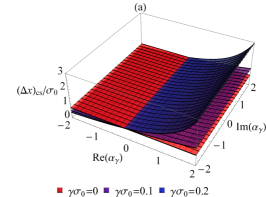
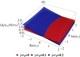
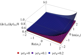
Figure 8: Uncertainties of (a) the position $(\Delta x)_{\textrm{cs}}$, (b) the linear momentum $(\Delta p)_{\textrm{cs}}$ and (c) the product $(\Delta x)_{\textrm{cs}}(\Delta p)_{\textrm{cs}}$ for the coherent states of the asymmetric deformed oscillator as function of the real and imaginary parts of $\alpha_{\gamma}$, with $\{|\textrm{Re}(\alpha_{\gamma})|,|\textrm{Im}(\alpha_{\gamma})|<2\}$. The surfaces are plotted for deformation parameter values $\gamma\sigma_{0}=0$ (usual case – red planes), $0.1$ (violet surfaces) and $0.2$ (blue surfaces).

In addition, the expected values of the superpotential ($\langle\hat{\Phi}_{\gamma}\rangle_{\textrm{cs}}$ and $\langle\hat{\Phi}_{\gamma}^{2}\rangle_{\textrm{cs}}$) and linear pseudomomentum ($\langle\hat{\Pi}_{\gamma}\rangle_{\textrm{cs}}$ and $\langle\hat{\Pi}_{\gamma}^{2}\rangle_{\textrm{cs}}$) for coherent states are

$$\langle\hat{\Phi}_{\gamma}\rangle_{\textrm{cs}} =\frac{\sigma_{0}}{\sqrt{2}}(\alpha_{\gamma}^{\ast}+\alpha_{\gamma}),$$ (87a)

$$\langle\hat{\Phi}_{\gamma}^{2}\rangle_{\textrm{cs}} =\frac{\sigma_{0}^{2}}{2}\left[1+(\alpha_{\gamma}^{\ast}+\alpha_{\gamma})^{2}-\frac{\gamma\sigma_{0}}{\sqrt{2}}(\alpha_{\gamma}^{\ast}+\alpha_{\gamma})-\frac{\gamma^{2}\sigma_{0}^{2}}{2}\right],$$ (87b)

$$\langle\hat{\Pi}_{\gamma}\rangle_{\textrm{cs}} =\frac{i\hbar}{\sqrt{2}\sigma_{0}}(\alpha_{\gamma}^{\ast}-\alpha_{\gamma}),$$ (87c)

$$\langle\hat{\Pi}_{\gamma}^{2}\rangle_{\textrm{cs}} =\frac{\hbar^{2}}{2\sigma_{0}^{2}}\left[1-(\alpha_{\gamma}^{\ast}-\alpha_{\gamma})^{2}-\frac{\gamma\sigma_{0}}{\sqrt{2}}(\alpha_{\gamma}^{\ast}+\alpha_{\gamma})-\frac{\gamma^{2}\sigma_{0}^{2}}{2}\right].$$ (87d)

It is easy to check that the results of a oscillator with constant mass are recovered: $\lim_{\gamma\rightarrow 0}\langle\hat{x}\rangle_{\textrm{cs}}=\lim_{\gamma\rightarrow 0}\langle\hat{\Phi}_{\gamma}\rangle_{\textrm{cs}}=\frac{\sigma_{0}}{\sqrt{2}}(\alpha_{0}^{\ast}+\alpha_{0})$, $\lim_{\gamma\rightarrow 0}\langle\hat{x}^{2}\rangle_{\textrm{cs}}=\lim_{\gamma\rightarrow 0}\langle\hat{\Phi}_{\gamma}^{2}\rangle_{\textrm{cs}}=\frac{\sigma_{0}^{2}}{2}[1+(\alpha_{0}^{\ast}+\alpha_{0})^{2}]$, $\lim_{\gamma\rightarrow 0}\langle\hat{p}\rangle_{\textrm{cs}}=\lim_{\gamma\rightarrow 0}\langle\hat{\Pi}_{\gamma}\rangle_{\textrm{cs}}=\frac{i\hbar}{\sqrt{2}\sigma_{0}}(\alpha_{0}^{\ast}-\alpha_{0})$ and $\lim_{\gamma\rightarrow 0}\langle\hat{p}^{2}\rangle_{\textrm{cs}}=\lim_{\gamma\rightarrow 0}\langle\hat{\Pi}_{\gamma}^{2}\rangle_{\textrm{cs}}=\frac{\hbar^{2}}{2\sigma_{0}^{2}}[1-(\alpha_{0}^{\ast}-\alpha_{0})^{2}]$.

From Eqs. (86) and (87), we readily obtain that the dispersions $(\Delta x)_{\textrm{cs}}^{2}=\langle\hat{x}^{2}\rangle_{\textrm{cs}}-\langle\hat{x}\rangle_{\textrm{cs}}^{2}$ and $(\Delta\Pi_{\gamma})_{\textrm{cs}}^{2}=\langle\hat{\Pi}_{\gamma}^{2}\rangle_{\textrm{cs}}-\langle\hat{\Pi}_{\gamma}\rangle_{\textrm{cs}}^{2}$ are expressed by

$$(\Delta x)_{\textrm{cs}}^{2} =\frac{\sigma_{0}^{2}}{2}\left(1+\gamma\langle\hat{x}\rangle_{\textrm{cs}}\right)^{2}\left(\frac{1}{1+\gamma\langle\hat{x}\rangle_{\textrm{cs}}}-\frac{\gamma^{2}\sigma_{0}^{2}}{2}\right)^{\!\!-1}$$ (88a)

$$(\Delta\Pi_{\gamma})_{\textrm{cs}}^{2} =\frac{\hbar^{2}}{2\sigma_{0}^{2}}\left(\frac{1}{1+\gamma\langle\hat{x}\rangle_{\textrm{cs}}}+\frac{\gamma^{2}\sigma_{0}^{2}}{2}\right)$$ (88b)

In the limit $|\alpha_{\gamma}|/\gamma\sigma_{0}\gg 1$ (or $\sigma_{0}\rightarrow 0$), we have that the squared of the deviations (88) behave like $(\Delta x)_{\textrm{cs}}^{2}\rightarrow\frac{\sigma_{0}^{2}}{2}(1+\gamma\langle\hat{x}\rangle_{\textrm{cs}})^{3}$ and $(\Delta\Pi_{\gamma})_{\textrm{cs}}^{2}\rightarrow\frac{\sigma_{0}^{2}}{2}(1+\gamma\langle\hat{x}\rangle_{\textrm{cs}})^{-1}$, so that $(\Delta x)_{\textrm{cs}}(\Delta\Pi_{\gamma})_{\textrm{cs}}=\frac{\hbar}{2}(1+\gamma\langle\hat{x}\rangle_{\textrm{cs}})$. Therefore, the coherent states minimize the generalized uncertainty relation between $\hat{x}$ and $\hat{\Pi}_{\gamma}$ (Eq. (31) for $g(\hat{x})=\hat{1}+\gamma\hat{x}$).

Because of the importance of the superpotential operator together with linear pseudomomentum in the factorization of $\hat{H}$, we also calculate, for the sake of completeness, the expected values $\langle\hat{\Phi}_{\gamma}\rangle$ and $\langle\hat{\Phi}_{\gamma}^{2}\rangle$ for the eigenstates $\psi_{n}(x)$, such that

$$\langle\hat{\Phi}_{\gamma}\rangle =n\gamma\sigma_{0}^{2},$$ (89a)

$$\langle\hat{\Phi}_{\gamma}^{2}\rangle =\sigma_{0}^{2}\left[(1-\gamma^{2}\sigma_{0}^{2})\left(n+\frac{1}{2}\right)+\frac{\gamma^{2}\sigma_{0}^{2}}{4}\right],$$ (89b)

whose mean square deviation is $(\Delta\Phi_{\gamma})^{2}=\sigma_{0}^{2}\left(n+\frac{1}{2}\right)\left[1-\gamma^{2}\sigma_{0}^{2}\left(n+\frac{1}{2}\right)\right].$ From Eqs. (44) and (89), the product of the uncertainties of $\hat{\Phi}_{\gamma}$ and $\hat{\Pi}_{\gamma}$ for the eigenstates satisfies

$$\Delta\Phi_{\gamma}\Delta\Pi_{\gamma} =\hbar\left(n+\frac{1}{2}\right)\left[1-\gamma^{2}\sigma_{0}^{2}\left(n+\frac{1}{2}\right)\right]$$

$$=\hbar\left(n+\frac{1}{2}\right)\left\langle\frac{1}{\hat{1}+\gamma\hat{x}}\right\rangle,$$ (90)

i.e., $\Delta\Phi_{\gamma}\Delta\Pi_{\gamma}\geq\frac{\hbar}{2}\left\langle\frac{1}{\hat{1}+\gamma\hat{x}}\right\rangle.$ On the other hand, from Eqs. (87) we arrive at

$$(\Delta\Phi_{\gamma})_{\textrm{cs}}(\Delta\Pi_{\gamma})_{\textrm{cs}} =\frac{\hbar}{2}\left[1-\frac{\gamma\sigma_{0}}{\sqrt{2}}(\alpha_{\gamma}^{\ast}+\alpha_{\gamma})-\frac{\gamma^{2}\sigma_{0}^{2}}{2}\right]$$

$$=\frac{\hbar}{2}\left\langle\frac{1}{\hat{1}+\gamma\hat{x}}\right\rangle_{\textrm{cs}}.$$ (91)

Thus, the coherent states minimize the uncertainty relation between the superpotential and the linear pseudomomentum in agreement with Ref. 52. In particular, the minimization of the uncertainty product $\Delta\Phi_{\gamma}\Delta\Pi_{\gamma}$ for the coherent states of the Morse oscillator was realized by Cooper through the algebraic method (see Ref. 69 for more details). Here, we verify that this property can also be extended to the asymmetric oscillator with PDM.

IV.4 Dynamics of quasi-classical states

In order to calculate the time evolution of coherent states $|\alpha_{\gamma}(t)\rangle$, let us start with the equation of motion of the operator $\hat{a}_{\gamma}$,

$$\frac{\textrm{d}}{\textrm{d}t}\hat{a}_{\gamma}=\frac{1}{i\hbar}[\hat{a}_{\gamma},\hat{H}]=-i\omega_{0}\left(\frac{1}{1+\gamma\hat{x}}\right)\hat{a}_{\gamma}.$$ (92)

Considering $\hat{a}_{\gamma}(t)=\hat{a}_{\gamma}(t_{0})e^{-i\Theta_{\textrm{cs},\gamma}(t)}$ the temporal rate of the phase $\Theta_{\textrm{cs},\gamma}(t)$ for coherent states becomes

$$\frac{\textrm{d}\Theta_{\textrm{cs},\gamma}(t)}{\textrm{d}t} =\omega_{0}\left\langle\frac{1}{\hat{1}+\gamma\hat{x}}\right\rangle_{\textrm{cs}}$$

$$=\omega_{0}\left[1-\sqrt{2}\gamma\sigma_{0}|\alpha_{\gamma}|\cos\Theta_{\textrm{cs},\gamma}(t)-\frac{\gamma^{2}\sigma_{0}^{2}}{2}\right],$$ (93)

with $\alpha_{\gamma}^{\ast}(t)+\alpha_{\gamma}(t)=2|\alpha_{\gamma}|\cos\Theta_{\textrm{cs},\gamma}(t)$ and $\Theta_{\textrm{cs},\gamma}(t_{0})=0$. Like the classic oscillator, by integrating Eq. (IV.4), we arrive at

$$\Theta_{\textrm{cs},\gamma}(t)=2\textrm{tan}^{-1}\left\{\sqrt{\frac{1-\sqrt{2}\gamma\sigma_{0}|\alpha_{\gamma}|-\frac{\gamma^{2}\sigma_{0}^{2}}{2}}{1+\sqrt{2}\gamma\sigma_{0}|\alpha_{\gamma}|-\frac{\gamma^{2}\sigma_{0}^{2}}{2}}}\textrm{tan}\left[\frac{1}{2}\Omega_{{\textrm{cs}},\gamma}(t-t_{0})\right]\right\}$$ (94)

and oscillation frequency $\Omega_{\textrm{cs},\gamma}=\omega_{0}\sqrt{\left(1-\frac{\gamma^{2}\sigma_{0}^{2}}{2}\right)^{2}-2\gamma^{2}\sigma_{0}^{2}|\alpha_{\gamma}|^{2}}.$

The temporal evolution of wavefunction $\Psi_{\textrm{cs}}(x,t)$ for coherent states is obtained by making the change $\alpha_{\gamma}\rightarrow\alpha_{\gamma}(t)=|\alpha_{\gamma}|e^{-i\Theta_{\textrm{cs},\gamma}(t)}$ in Eqs. (85) with the deformed phase $\Theta_{\textrm{cs},\gamma}(t)$ given by Eq. (94). In figure 9 we plot three frames of the motion of the probability density $|\Psi_{\textrm{cs}}(x,t)|^{2}$ with the deformation parameter $\gamma\sigma_{0}=0$ (standard oscillator) and $0.4$.

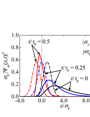
Figure 9: Snapshots of the probability density $|\Psi_{\textrm{cs}}(x,t)|^{2}$ for coherent states $|\alpha_{\gamma}\rangle$ of the asymmetric oscillator with PDM and deformation parameter $\gamma\sigma_{0}=0.4$ and $|\alpha_{\gamma}|=1/\sqrt{2}$. The frames are represented at the times $t=0$, $\tau_{0}/4$ and $\tau_{0}/2$ ($\tau_{0}=2\pi/\omega_{0}$). The usual case ($\gamma=0$, dashed-dotted line) is also shown for comparison.

Since $\textrm{Re}[\alpha_{\gamma}(t)]=|\alpha_{\gamma}|\cos\Theta_{\gamma}(t)$ and $\textrm{Im}[\alpha_{\gamma}(t)]=|\alpha_{\gamma}|\sin\Theta_{\gamma}(t),$ from Eqs. (86a), (86c) and (87c) we can express the time evolution of the expected values of the position, the linear momentum and the linear pseudomomentum as

$$\langle\hat{x}(t)\rangle_{\textrm{cs}} =\frac{A_{\textrm{cs}}\cos\Theta_{\textrm{cs},\gamma}(t)+\gamma\sigma_{0}^{2}}{1-\gamma A_{\textrm{cs}}\cos\Theta_{\textrm{cs},\gamma}(t)-\gamma^{2}\sigma_{0}^{2}},$$ (95a)

$$\langle\hat{p}(t)\rangle_{\textrm{cs}} =-m_{0}\omega_{0}A_{\textrm{cs}}\sin{\Theta_{\textrm{cs},\gamma}}(t)\left[1-\gamma A_{\textrm{cs}}\cos\Theta_{\textrm{cs},\gamma}(t)-\frac{\gamma^{2}\sigma_{0}^{2}}{2}\right]$$ (95b)

$$\langle\hat{\Pi}_{\gamma}(t)\rangle_{\textrm{cs}} =-m_{0}\omega_{0}A_{\textrm{cs}}\sin{\Theta_{\textrm{cs},\gamma}}(t)$$ (95c)

with $A_{\textrm{cs}}=\sqrt{2}\sigma_{0}|\alpha_{\gamma}|$ being an amplitude oscillation for the coherent states. As predicted, $\langle\hat{x}(t)\rangle_{\textrm{cs}}$, $\langle\hat{p}(t)\rangle_{\textrm{cs}}$ and $\langle\hat{\Pi}_{\gamma}(t)\rangle_{\textrm{cs}}$ for $A_{\textrm{cs}}/\sigma_{0}\gg 1$ (or $|\alpha_{\gamma}|\gg 1$) evolve over time in the same way as their respective classical analog [Eqs. (12), (15) and (19b)]. A correspondence between the temporal evolution for the expected values of the coherent states and their trajectory in classical formalism was previously obtained by Kais and Levine for the Morse oscillator.[68] Here, we realize that the correspondence is valid for the asymmetric oscillator with PDM.

From Eqs. (86a)–(86d) with $\alpha_{\gamma}(t)=|\alpha_{\gamma}|e^{-i\Theta_{\gamma}(t)}$ and deformed phase (94), we present in Fig. 10 the time evolution of the uncertainties of the position $(\Delta x)_{\textrm{cs}}(t)=\sqrt{\langle\hat{x}^{2}(t)\rangle_{\textrm{cs}}-\langle\hat{x}(t)\rangle_{\textrm{cs}}^{2}},$ the linear momentum $(\Delta p)_{\textrm{cs}}(t)=\sqrt{\langle\hat{p}^{2}(t)\rangle_{\textrm{cs}}-\langle\hat{p}(t)\rangle_{\textrm{cs}}^{2}},$ and the product $(\Delta x)_{\textrm{cs}}(t)(\Delta p)_{\textrm{cs}}(t)$ for coherent states of the asymmetric oscillator with different values of $\gamma\sigma_{0}$. The standard case ($\gamma=0$) [$(\Delta x)_{\textrm{cs}}(t)=\frac{\sigma_{0}}{\sqrt{2}}$, $(\Delta p)_{\textrm{cs}}(t)=\frac{\hbar}{\sqrt{2}\sigma_{0}}$ and $(\Delta x)_{\textrm{cs}}(t)(\Delta p)_{\textrm{cs}}(t)=\frac{\hbar}{2}$] is shown for comparison.

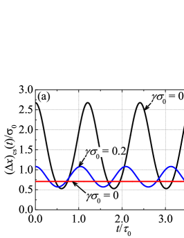
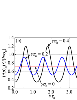
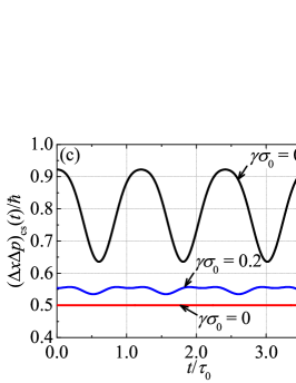
Figure 10: Time evolution of the uncertainties of (a) the position $(\Delta x)_{\textrm{cs}}(t)$ and (b) the linear momentum $(\Delta p)_{\textrm{cs}}(t)$, and (c) of the product $(\Delta x)_{\textrm{cs}}(t)(\Delta p)_{\textrm{cs}}(t)$ for the coherent states of the asymmetric oscillator with PDM, with $|\alpha_{\gamma}|=1/\sqrt{2}$ and deformation parameters $\gamma\sigma_{0}=0$ (usual case), $0.2$ (dashed red) and $0.4$ (dashed-dotted blue).

As a final application, let $\psi_{\pm\alpha_{\gamma}}(x)=\langle{x}|{\pm\alpha_{\gamma}}\rangle$ be the wavefunctions of the corresponding states $|\pm\alpha_{\gamma}\rangle$ in position representation $\{|\hat{x}\rangle\}$, and the even and odd coherent states are given by [74, 75]

$$\psi_{\textrm{even}}(x) =C_{\textrm{even}}[\psi_{\alpha_{\gamma}}(x)+\psi_{-\alpha_{\gamma}}(x)],$$ (96a)

$$\psi_{\textrm{odd}}(x) =C_{\textrm{odd}}[\psi_{\alpha_{\gamma}}(x)-\psi_{-\alpha_{\gamma}}(x)].$$ (96b)

with the normalization constants given by

$$\left\{\begin{array}[]{c}C_{\textrm{even}}\\ C_{\textrm{odd}}\end{array}\right\}=\frac{1}{2[1\pm\langle-\alpha_{\gamma}|\alpha_{\gamma}\rangle]}.$$ (97)

For the deformed oscillator, we obtain that the inner product $\langle-\alpha_{\gamma}|\alpha_{\gamma}\rangle=\int_{-\infty}^{\infty}\psi_{-\alpha_{\gamma}}^{\ast}(x)\psi_{\alpha_{\gamma}}(x)\textrm{d}x$ is expressed as

$$\langle-\alpha_{\gamma}|\alpha_{\gamma}\rangle=\sqrt{\frac{B(\widetilde{\lambda}_{\textrm{cs}}(\alpha_{\gamma}),\widetilde{\lambda}_{\textrm{cs}}(-\alpha_{\gamma}))}{B(\lambda_{\textrm{cs}}(\alpha_{\gamma}),\lambda_{\textrm{cs}}(-\alpha_{\gamma}))}},$$ (98)

whose arguments are $\lambda_{\textrm{cs}}(\alpha_{\gamma})=\frac{2}{\gamma^{2}\sigma_{0}^{2}}[1-\sqrt{2}\gamma\sigma_{0}\textrm{Re}(\alpha_{\gamma})]-1$ and $\widetilde{\lambda}_{\textrm{cs}}(\alpha_{\gamma})=\frac{2}{\gamma^{2}\sigma_{0}^{2}}[1-i\sqrt{2}\gamma\sigma_{0}\textrm{Im}(\alpha_{\gamma})]-1.$ For $\gamma=0$ , we recover the standard case $\lim_{\gamma\rightarrow 0}\langle-\alpha_{\gamma}|\alpha_{\gamma}\rangle=e^{-2|\alpha_{0}|^{2}}$.

The temporal evolution $\Psi_{\textrm{even}}(x,t)$ and $\Psi_{\textrm{odd}}(x,t)$ of the coherent states are obtained by changing $\alpha_{\gamma}\rightarrow\alpha_{\gamma}(t)=|\alpha_{\gamma}|e^{-i\Theta_{\textrm{cs},\gamma}(t)}$ in Eqs. (96). In figure 11 we plot the density probabilities $\rho_{\textrm{even}}(x,t)=|\Psi_{\textrm{even}}(x,t)|^{2}$ and $\rho_{\textrm{odd}}(x,t)=|\Psi_{\textrm{odd}}(x,t)|^{2}$ for different values of the parameters $\alpha_{\gamma}$ and $\gamma\sigma_{0}$.

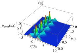
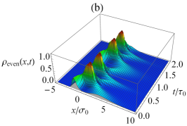
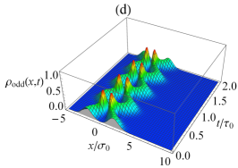
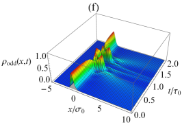
Figure 11: Probability behavior of even (upper line) and odd (bottom line) coherent states with $|\alpha_{\gamma}|=\sqrt{2}$ and $\gamma\sigma_{0}=0$ [(a) and (d) – standard case], $\gamma\sigma_{0}=0.1$ [(b) and (e)], and $\gamma\sigma_{0}=0.2$ [(c) and (f)].

V Final remarks

In this work, we have addressed the properties of a classical and quantum deformed oscillator provided with an asymmetrical position-dependent mass $m(x)=m_{0}/(1+\gamma x)^{2}$ in the harmonic potential term of the Hamiltonian. As a continuation of our previous work (Ref. 61), we obtain eigenfunctions, energy levels, mean values, coherent states, and uncertainty relationships. We summarize our contributions as follows: (i) The classical and quantum Hamiltonians of the deformed oscillator result equivalent to the Morse oscillator Hamiltonian expressed in the deformed space due to the introduction of the position-dependent mass $m(x)=m_{0}/(1+\gamma x)^{2}$ in the potential term given by $V(x)=\frac{1}{2}m(x)\omega_{0}^{2}x^{2}$. (ii) The evolution of the mean values of the position and the momentum remains as its oscillatory character, but the phase space deforms continuously and asymmetrically from a circle (null deformation) to a closed curve with peaks (Fig. 1). In addition, the wavefunctions and their probability functions result asymmetrical around $x=0$. (iii) For large values of the quantum number $n$, the classical limit is recovered (Fig. 3). (iv) Uncertainty relationships have a lower bound that increases as the deformation increases (Fig. 5).

Overall, there exist two controlled ways to introduce a deformation in the context of the harmonic oscillator Hamiltonian: (1) by means of a deformation in the momentum $p\rightarrow p_{\gamma}$ and (2) through a deformation in the harmonic potential $V_{0}(x)=\frac{1}{2}m_{0}\omega_{0}^{2}x^{2}\rightarrow V(x)=\frac{1}{2}m(x)\omega_{0}^{2}x^{2}$. By employing both (1) and (2) we have shown that, analogously to the accomplished in Ref. 61, the deformation affects the stationary aspects, expressed by the asymmetry of the energies and eigenfunctions and the increasing lower bounds of the uncertainty relationships as well as the temporal aspects regarding the localization of the probability distributions of the eigenfunctions and the oscillations of the uncertainty relationships. It remains to be seen whether this is due to the fact that the same position-dependent mass was used in the momentum and in the potential, which we hope will be studied future research.

We also investigate the coherent states of the deformed oscillator. The probability density of the coherent states localizes rapidly regarding the oscillation period $\tau_{0}=2\pi/\omega_{0}$ because of the effect of the asymmetrical deformation provided by the PDM (Fig 6). As previously predicted in the literature for coherent states of the Morse oscillator (see Ref. 72) — system equivalent to the PDM oscillator that we study here— the uncertainty principle is also satisfied for the deformed oscillator. Periodic oscillations in the time evolution of the uncertainty relationships arise as the dimensionless deformation parameter $\gamma\sigma_{0}$ increases (Fig 7). In addition, as in the Morse oscillator,[68] the time evolution of the observable position and linear momentum for the coherent states reproduce their respective classical analogs.

We have limited this work in investigating Glauber’s coherent states for the deformed oscillator. However, the investigation of generalized coherent states for systems with PDM can be obtained from the approaches of Klauder and Sudarshan,[3, 4, 5] Barut and Girardello,[6, 71] Gazeau–Klauder,[70] and Perelomov,[7, 67] quantum anomaly in the systems with the second order supersymmetry,[65] generalized Heisenberg algebras,[73] and conformal quantum mechanical[76] in interesting additional developments. A group theoretical approach to the deformed oscillator, including both bound and scattering, can be obtained in future developments from the formalism introduced in Ref. 77 and applied to the Morse oscillator.

References

References

- [1] E. Schrödinger, Naturwissenschaften 14(28), 664 (1926).
- [2] R. J. Glauber, Phys. Rev. 131(6), 2766 (1963).
- [3] J. R. Klauder, J. Math. Phys. 4(8), 1055 (1963).
- [4] J. R. Klauder, J. Math. Phys. 4(8), 1058 (1963).
- [5] E. C. G. Sudarshan, Phys. Rev. Lett. 10, 277 (1963).
- [6] A. O. Barut and L. Girardello, Commun. Math. Phys. 21, 41 (1971).
- [7] A. M. Perelomov, Commun. Math. Phys. 26, 222 (1972).
- [8] J. P. Gazeau, Coherent States in Quantum Physics (Wiley–VCH, 2009).
- [9] C. Gerry and P. L. Knight, Introductory Quantum Optics (Cambridge University Press, 2005).
- [10] C. Monroe, D. M. Meekhof, B. E. King, and D. J. Wineland, Science, 272(5265), 1131 (1996).
- [11] A. Laghaout, J. S. Neergaard-Nielsen, I. Rigas, C. Kragh, A. Tipsmark, and U. L. Andersen, Phys. Rev. A 87(4), 043826 (2013).
- [12] L. G. Lutterbach and L. Davidovich, Phys. Rev. Lett. 78(13), 2547 (1997).
- [13] A. Aragão, A. T. Avelar, and B. Baseia, Phys. Lett. A 331(6), 366-373 (2004).
- [14] A. Zavatta, V. Parigi, and M. Bellini, Phys. Rev. A 75(5), 052106 (2007).
- [15] D. F. Walls, Nature 306(5939), 141 (1983).
- [16] G. Bastard, J. K. Furdyna, and J. Mycielski, Phys. Rev. B 12, 4356 (1975).
- [17] O. von Roos, Phys. Rev. B 27, 7547 (1983).
- [18] D. J. BenDaniel and C. B. Duke, Phys. Rev. 152, 683 (1966).
- [19] T. Gora and F. Williams, Phys. Rev. 177, 1179 (1969).
- [20] Q.-G. Zhu and H. Kroemer, Phys. Rev. B 27, 3519 (1983).
- [21] T. L. Li and K. J. Kuhn, Phys. Rev. B 47, 12760 (1993).
- [22] R. A. Morrow and K. R. Brownstein, Phys. Rev. B 30, 678 (1984).
- [23] O. Mustafa and S. H. Mazharimousavi, Int. J. Theor. Phys. 46, 1786 (2007).
- [24] K. Li, K. Guo, X. Jiang, M. Hu, Optik 132, 375 (2017).
- [25] F. Arias de Saavedra, J. Boronat, A. Polls, and A. Fabrocini, Phys. Rev. B 50, 4248 (1994).
- [26] K. Bencheikh, K. Berkane and S. Bouizane, J. Phys. A: Math. Gen. 37 (45), 10719 (2004).
- [27] J. Yu, S.-H. Dong, and G.-H. Sun, Phys. Lett. A 322, 290 (2004).
- [28] H. R. Christiansen and M. S. Cunha, J. Math. Phys. 55, 092102 (2014).
- [29] G. Yañez-Navarro, G.-H. Sun, T. Dytrych, K. D. Launey, S.-H. Dong, and J. P. Draayer, Ann. Phys. 348 153 (2014).
- [30] O. Aydoǧdu, A. Arda, and R. Sever, J. Math. Phys. 53, 042106 (2012).
- [31] A. Merad, M. Aouachria, M. Merad, and T. Birkandan, Int. J. Mod. Phys. A 34(32), 1950218 (2019).
- [32] M. Alimohammadi, H. Hassanabadi, and S. Zare, Nucl. Phys. A 960, 78 (2017).
- [33] A. G. M. Schmidt and A. L. de Jesus, J. Math. Phys. 59, 102101 (2018).
- [34] A. L. de Jesus and A. G. M. Schmidt, J. Math. Phys. 60, 122102 (2019).
- [35] P. M. Mathews and M. Lakshmanan, Q. Appl. Math. 32, 215 (1974).
- [36] P. M. Mathews and M. Lakshmanan, Nuovo Cimento A 26, 299 (1975).
- [37] A. K. Tiwari, S. N. Pandey, M. Senthilvelan, and M. Lakshmanan, J. Math. Phys. 54(5), 053506 (2013).
- [38] B. Bagchi, A. Ghose Choudhury, and P. Guha, J. Math. Phys. 56, 012105 (2015).
- [39] J. F. Cariñena, M. F. Rañada, and M. Santander, Ann. Phys. 322, 434 (2007).
- [40] V. Chithiika Ruby, V. K. Chandrasekar, M. Senthilvelan, and M. Lakshmanan, J. Math. Phys. 56, 012103 (2015).
- [41] A. Schulze-Halberg and B. Roy, J. Math. Phys. 57, 102103 (2016).
- [42] S. Karthiga, V. Chithiika Ruby, M. Senthilvelan, and M. Lakshmanan, J. Math. Phys. 58, 102110 (2017).
- [43] C. Quesne, Eur. Phys. J. Plus 137, 225 (2022).
- [44] E. I. Jafarov, S. M. Nagiyev, and A. M. Jafarova, Rep. Math. Phys. 86, 25 (2020).
- [45] E. I. Jafarov and J. Van der Jeugt, Eur. Phys. J. Plus 136, 758 (2021).
- [46] E. I. Jafarov, Physica E 139, 115160 (2022).
- [47] A. R. Plastino, A. Rigo, M. Casas, F. Garcias, and A. Plastino, Phys. Rev. A 60(6), 4318 (1999).
- [48] R. Bravo and M. S. Plyushchay, Phys. Rev. D 93, 105023 (2016).
- [49] N. Amir and S. Iqbal, J. Math. Phys. 57, 062105 (2016).
- [50] S. Karthiga, V. Chithiika Ruby,, and M. Senthilvelan, Phys. Lett. A 382(25), 1645 (2018).
- [51] O. Mustafa, Phys. Lett. A 384, 126265 (2020).
- [52] V. Chithiika Ruby and M. Senthilvelan, J. Math. Phys. 51, 052106 (2010).
- [53] N. Amir and S. Iqbal, J. Math. Phys. 56, 062108 (2015).
- [54] N. Amir and S. Iqbal, Commun. Theor. Phys. 66, 615 (2016).
- [55] M. Tchoffo, F. B. Migueu, M. Vubangsi, and L. C. Fai, Heliyon 5(9), e02395 (2019).
- [56] R. N. Costa Filho, M. P. Almeida, G. A. Farias, and J. S. Andrade Jr., Phys. Rev. A 84, 050102(R) (2011).
- [57] R. N. Costa Filho, G. Alencar, B.-S. Skagerstam, and J. S. Andrade Jr., Europhys. Lett. 101, 10009 (2013).
- [58] V. Aguiar, S. M. Cunha, D. R. da Costa, R. N. Costa Filho, Phys. Rev. B 102, 235404 (2020).
- [59] B. G. da Costa and E. P. Borges, J. Math. Phys. 55, 062105 (2014).
- [60] B. G. da Costa and E. P. Borges, J. Math. Phys. 59, 042101 (2018).
- [61] B. G. da Costa, G. A. C. da Silva, I. S. Gomez J. Math. Phys. 62, 092101 (2021).
- [62] B. G. da Costa, I. S. Gomez, and M. Portesi, J. Math. Phys. 61, 082105 (2020).
- [63] N. Jamshir, B. Lari, and H. Hassanabadi, Physica A 565, 125616 (2021).
- [64] S. Cruz y Cruz and C. Santiago-Cruz Math. Methods Appl. Sci. 42, 4909 (2019).
- [65] M. S. Plyushchay, Ann. Phys. 377, 164 (2017).
- [66] M. M. Nieto and L. M. Simmons Jr, Phys. Rev. D 20, 1342 (1979).
- [67] A. Perelomov, Generalized Coherent States (Springer, Berlin, 1986).
- [68] S. Kais and R. D. Levine, Phys. Rev. A 41, 2301 (1990).
- [69] I. L. Cooper, J. Phys. A: Math. Gen. 25 1671 (1992).
- [70] B. Roy and P. Roy, Phys. Lett. A 296(4-5) 187 (2002).
- [71] D. Popov, S.-H. Dong, N. Pop, V. Sajfert, and S. Şimon, Ann. Phys. 339, 122 (2013).
- [72] M. Angelova and V. Hussin, J. Phys. A: Math. Theor. 41(30), 304016 (2008).
- [73] A. Belfakir, Y. Hassouni, and E. M. F. Curado Phys. Lett. A 384, 126553 (2020).
- [74] V. V. Dodonov, I. A. Malkin, and V. I. Man’ko, Physica 72(3), 597 (1974).
- [75] V. Bužek, A. Vidiella-Barranco, and P. L. Knight, Phys. Rev. A 45, 6570 (1992).
- [76] L. Inzunza, M. S. Plyushchay, A. Wipf, Phys. Rev. D 101, 105019 (2020).
- [77] Y. Alhassid, F. Iachello, and F. Gürsey, Chem. Phys. Lett. 99(1), 27 (1983).