A hybrid stochastic configuration interaction–coupled cluster approach for multireference systems

Abstract

The development of multireference coupled cluster (MRCC) techniques has remained an open area of study in electronic structure theory for decades due to the inherent complexity of expressing a multi-configurational wavefunction in the fundamentally single-reference coupled cluster framework. The recently developed multireference coupled cluster Monte Carlo (mrCCMC) technique uses the formal simplicity of the Monte Carlo approach to Hilbert space quantum chemistry to avoid some of the complexities of conventional MRCC, but there is room for improvement in terms of accuracy and, particularly, computational cost. In this paper we explore the potential of incorporating ideas from conventional MRCC — namely the treatment of the strongly correlated space in a configuration interaction formalism — to the mrCCMC framework, leading to a series of methods with increasing relaxation of the reference space in the presence of external amplitudes. These techniques offer new balances of stability and cost against accuracy, as well as a means to better explore and better understand the structure of solutions to the mrCCMC equations.

I Introduction

Generally, ab initio wavefunction based electronic structure methods aim to include electron correlation effects unaccounted for in a zeroth order wavefunction such as that obtained from a self-consistent field (SCF) approximation. These effects are commonly split into dynamic and static correlation, with largely distinct physical origins. While the former can be successfully treated by coupled cluster (CC) theory, in particular the ever-popular CCSD(T)Raghavachari et al. (1989) approach, the latter induces a strongly multi-configurational wavefunction, which cannot be easily described by the exponential CC Ansatz.

The most commonly used approaches combine different algorithms to solve the static and dynamic correlation problems independently: a complete active space self-consistent field (CASSCF) calculation aims to capture the static correlation in the system, while a many-body perturbation theory (MBPT) calculation is used to include remaining dynamic correlation. Depending on the Hamiltonian partitioning used, this leads to methods like complete active-space second-order perturbation theory (CASPT2)Andersson et al. (1990) and $n$-electron valence perturbation theory (NEVPT) Angeli et al. (2001); Angeli, Cimiraglia, and Malrieu (2001, 2002).

The treatment of strong static correlation using coupled cluster methods remains an area of active research. Numerous multireference coupled cluster (MRCC) methods have been developed to tackle this problem, using both state-universal approaches, which compute multiple electronic states of the system simultaneously, and state-specific ones, which target one state at a time (see Lyakh et al., 2011 for a review of such methods). Generally, MRCC techniques have not achieved the same popularity as their single-reference counterpart due to various challenges with size-consistency,Lyakh et al. (2011) intruder statesKaldor (1988); Paldus et al. (1993); Jankowski and Malinowski (1994); Piecuch and Paldus (1994) and the higher system-specific knowledge requirement to use them effectively. An alternative approach has been to use externally corrected coupled cluster methods,Paldus (2017) which make use of approximations to higher order cluster amplitudes from other sources such as adaptive configuration interaction (ACI)Schriber and Evangelista (2016) or full configuration interaction quantum Monte Carlo (FCIQMC) and coupled cluster Monte Carlo (CCMC).Deustua, Shen, and Piecuch (2017); Deustua et al. (2018); Deustua, Shen, and Piecuch (2021) Finally, the tailored coupled cluster methods use amplitudes from another method, such as CASCIKinoshita, Hino, and Bartlett (2005); Mörchen, Freitag, and Reiher (2020); Vitale, Alavi, and Kats (2020) or the density matrix renormalization group (DMRG) methodVeis et al. (2016), to include non-dynamical correlation into a single-reference coupled cluster calculation, during which these initial amplitudes are kept fixed.

FCIQMCBooth, Thom, and Alavi (2009) and CCMCThom (2010) are stochastic alternatives to traditional ab initio methods which have been developed in the last decade to take advantage of the sparsity present in most electronic Hamiltonians to significantly decrease calculation memory requirements. The CCMC algorithm also permits easy generalisation to large cluster truncation levels,Neufeld and Thom (2017) which allows high-accuracy calculations for systems with significant contributions from highly excited determinants. While simple to implement, these methods can still be computationally prohibitive, scaling as $\mathcal{O}(N^{2n+2})$, where $N$ is a measure of system size and $n$ is the cluster expansion truncation level. We recently developed a state-specific multireference CCMCFilip, Scott, and Thom (2019) approach that is highly flexible, using an arbitrary reference space and potentially distinct truncation levels with respect to each reference. These properties can be used to define optimised calculations but doing so requires careful advance investigation of the system’s Hilbert space, which can be time- and resource-consuming for large systems. A common approach employed in MRCC methods is to use a complete active space (CAS) as a reference space and initialise it with a high accuracy method such as CASCI or CASSCF. While this is not necessarily always the optimal reference, it requires minimal system-specific knowledge to implement.

In this paper, we investigate ways of combining a configuration interaction quantum Monte Carlo (CIQMC) calculation in a CAS with a multireference CCMC calculation to treat the external space. We develop schemes allowing increasing relaxation of the CASCIQMC wavefunction in the presence of the external mr-CCMC contributions and explore their properties using a minimal basis square H₄ model, as well as the 4- and 8-site 2D Hubbard model. We also use a range of toy Li systems to explore the performance of each approach as the number of core and virtual orbitals increases.

II Quantum Monte Carlo Methods

II.1 Full Configuration Interaction Quantum Monte Carlo

FCIQMCBooth, Thom, and Alavi (2009) encodes a stochastic solution to the FCI equations. The FCI wavefunction is expressed as a linear combination of Slater determinants, generally obtained by considering all possible arrangements of the desired number of electrons among spin-orbitals obtained from a Hartree–Fock (HF) calculation.

$$\ket{\Psi_{\mathrm{FCI}}}=(1+\hat{C})\ket{D_{0}}$$ (1)

where $\ket{D_{0}}$ is the Hartree–Fock reference determinant, $\hat{C}=\sum_{i,a}c_{i}^{a}\hat{a}_{i}^{a}+\frac{1}{4}\sum_{i,j,a,b}c_{ij}^{ab}\hat{a}_{ij}^{ab}+...$ and $\hat{a}_{i}^{a},\hat{a}_{ij}^{ab}$ are excitation operators, exciting electrons from spin-orbitals $i,j,...$ to spin-orbitals $a,b,...$.

FCIQMC belongs to the family of Projector Monte Carlo (PMC) methods, in which the ground state wavefunction is obtained by solving the imaginary time Schrödinger equation,

$$\frac{\partial\ket{\Psi}}{\partial\tau}=-\hat{H}\ket{\Psi},$$ (2)

where $\tau$ is imaginary time and $\hat{H}$ is the Hamiltonian of the system of interest. This has a solution of the form

$$\ket{\Psi_{0}}=\lim_{\tau\rightarrow\infty}e^{-\tau(\hat{H}-E_{0})}\ket{\Psi(0)},$$ (3)

where $\ket{\Psi(0)}$ is some initial trial wavefunction such that $\braket{\Psi_{0}}{\Psi(0)}\neq 0$ and $E_{0}$ is the lowest eigenvalue of $\hat{H}$. The imaginary-time interval can be split into a series of small time-steps $\delta\tau$ and eq. 3 can be rewritten in an iterative form as

$$\ket{\Psi(\tau+\delta\tau)}=e^{-\delta\tau(\hat{H}-E_{0})}\ket{\Psi(\tau)}\approx(1-\delta\tau(\hat{H}-E_{0}))\ket{\Psi(\tau)}.$$ (4)

If $\ket{\Psi(\tau)}$ is an FCI wavefunction, projection of the equation above onto all the determinants in the Hilbert space, $\bra{D_{\mu}}=\bra{D_{0}}(\hat{a}_{ij...}^{ab...})^{\dagger}$, gives an iterative update equation for the CI coefficients,

$$c_{\mu}(\tau+\delta\tau)=c_{\mu}(\tau)\underbrace{-\vphantom{\sum_{\nu}}\delta\tau\braket{D_{\mu}}{\hat{H}-E_{0}}{D_{\mu}}c_{\mu}(\tau)}_{\mathrm{Death}}\underbrace{-\sum_{\nu}\delta\tau\braket{D_{\mu}}{\hat{H}}{D_{\nu}}c_{\nu}(\tau)}_{\mathrm{Spawning}}.$$ (5)

The CI coefficients on each determinant can be viewed as populations of psips (‘psi particles’ or ‘walkers’) residing in the Hilbert space of the system. Equation 5 can be solved stochastically by sampling the population dynamics of the psips as they undergo the following processes:

• spawning from $\ket{D_{\nu}}$ to $\ket{D_{\mu}}$ creates a new particle with probability

  $$p_{\mathrm{spawn}}(\nu|\mu)\propto\delta\tau|H_{\mathbf{\mu\nu}}|;$$ (6)

• death or cloning of particles on $\ket{D_{\mu}}$ occurs with probability

  $$p_{\mathrm{death}}(\mu)\propto\delta\tau|H_{\mathbf{\mu\mu}}-S|,$$ (7)

  where the parameter $S$, known as the shift, has been introduced in place of the unknown ground state energy $E_{0}$.

• annihilation of particles of opposite sign on the same determinant.

The shift in the death step is allowed to vary, acting as a population control parameter and, once the system has reached a steady state, converges to the true energy $E_{0}$. In a standard FCIQMC calculation, two independent estimators can therefore be used for the energy – the shift described above and the projected energy

$$E_{\mathrm{proj}}=\frac{\braket{D_{0}}{\hat{H}}{\Psi}}{\braket{D_{0}}{\Psi}}=\sum_{\mu\neq 0}\frac{N_{\mu}H_{\mu 0}}{N_{0}},$$ (8)

where $N_{\mu}$ is the FCIQMC population on determinant $\mu$, which should on average be proportional to $c_{\mu}$. Effective techniques to obtain statistical estimates of these quantities from the QMC imaginary-time series have been devisedIchibha et al. (2022) and for large enough particle populations they are unbiased estimators of the true energy. For low populations, a bias is observed but can be minimised by using appropriate calculation parameters.Vigor et al. (2015)

II.2 Coupled Cluster Monte Carlo

Rather than a CI expansion, one can use a CC exponential Ansatz for the QMC trial wavefunction.

$$\ket{\Psi_{\mathrm{CC}}}=e^{\hat{T}}\ket{D_{0}}$$ (9)

where $\hat{T}=\sum_{i,a}t_{i}^{a}\hat{a}_{i}^{a}+\frac{1}{4}\sum_{i,j,a,b}t_{ij}^{ab}\hat{a}_{ij}^{ab}+...$.

When the system is dominated by dynamic correlation, the HF reference is a good first-order approximation to the true wavefunction, so we expect the cluster amplitudes $\{\mathbf{t}\}$ to be small. Hence $\braket{D_{\mu}}{\Psi_{\mathrm{CC}}}=t_{\mu}+\mathcal{O}(t^{2})$ and we can write

$$t_{\mu}(\tau)-\delta\tau\braket{D_{\mu}}{\hat{H}-E_{0}}{\Psi_{\mathrm{CC}}}\approx t_{\mu}(\tau+\delta\tau).$$ (10)

This equation can be described by the same population dynamics considered for FCIQMC, using once again a variable shift to estimate the unknown ground state energy $E_{0}$, but one must take into consideration contributions from “composite clusters", where we define a cluster to be any combination of excitation operators that appears in the expansion of the coupled cluster exponential Ansatz. For example,

$$\braket{D_{ij}^{ab}}{\Psi_{\mathrm{CC}}}=\underbrace{t_{ij}^{ab}}_{\mathrm{non-composite\ cluster}}+\underbrace{t_{i}^{a}t_{j}^{b}-t_{i}^{b}t_{j}^{a}}_{\mathrm{composite\ clusters}},$$ (11)

and therefore any of these three terms may contribute to death on $t_{ij}^{ab}$ or to spawning onto some excitor coupled to it by the Hamiltonian. The selection process for terms in eq. 10 is therefore somewhat more complicated than for FCIQMC. The original selection algorithm begins by selecting a cluster size $s$ with probability

$$p(s)=\begin{cases}\frac{1}{2^{s+1}},&s<s_{\mathrm{max}}\\ \frac{1}{2^{s}},&s=s_{\mathrm{max}}.\end{cases}$$ (12)

A particular cluster of $s$ distinct excitation operators or excitors is then selected with probability

$$p(e|s)=s!\prod_{i=1}^{s}\frac{|N_{i}|}{|N_{\mathrm{ex}}|}$$ (13)

where $N_{\mathrm{ex}}$ is the total population on excitors. The total selection probability is therefore

$$p_{\mathrm{sel}}(e)=p(e|s)p(s)=\frac{s!\prod_{i=1}^{s}\frac{|N_{i}|}{|N_{\mathrm{ex}}|}}{2^{s+1}}$$ (14)

Once this cluster is selected, the determinant obtained by applying it to the reference determinant must be computed, so that it may be used in the stochastic processes described previously. However, care must be taken to account for potential sign differences between the cluster representation of a determinant, $\prod_{e}\hat{a}_{e}\ket{D_{0}}$ and the determinant itself $\ket{D_{ij...}^{ab...}}$. due to the commutation properties of the excitation operators.

Various improvements have been developed for the CCMC algorithm,Franklin et al. (2016); Spencer and Thom (2016); Neufeld and Thom (2019); Spencer et al. (2018) including an importance-sampling-based selection method, which avoids the disproportionately high likelihood of selection of unimportant large clusters in the original method.Scott and Thom (2017)

II.3 Multireference Coupled Cluster Monte Carlo

For a multireference coupled cluster approach, the Hilbert space can be partitioned into a reference (model) space and an external space. One approach, first suggested in the work or Piecuch, Oliphant and Adamowicz,Oliphant and Adamowicz (1991, 1992); Piecuch, Oliphant, and Adamowicz (1993); Piecuch and Adamowicz (1994) uses a formally single-reference Ansatz,

$$\ket{\Psi_{\mathrm{CC}}}=e^{\hat{T}_{\mathrm{int}}+\hat{T}_{\mathrm{ext}}}\ket{D_{0}},$$ (15)

where $\hat{T}_{\mathrm{int}}$ excite electrons within the reference space while $\hat{T}_{\mathrm{ext}}$ includes at least one external excitation. Given a principal reference $\ket{D_{0}}$ each other determinant in the reference space (referred to as ‘secondary references’ in the following) can be expressed as $\ket{D_{n}}=\pm\hat{a}_{n}\ket{D_{0}}$, where $\hat{a}_{n}$ is some excitation operator, we can also express a multireference coupled cluster wavefunction as

$$\ket{\Psi_{\mathrm{CC}}}=\mathrm{exp}[\sum_{i=1}^{m_{0}}\hat{T}_{i}+\sum_{n=1}^{N}\sum_{j=0}^{m_{n}}\hat{T}^{(n)}_{j}t_{n}\hat{a}_{n}]\ket{D_{0}},$$ (16)

where $\hat{T}_{i}$ are external $i$-th order excitors of the first reference, $\hat{T}^{(n)}_{j}$ are external $j$-th order excitors of the $n$-th secondary reference, $m_{n}$ is the truncation level associated with each reference and $t_{m}$ are the coefficients of the internal excitation operators. This form allows for a completely general reference space and set of excitation levels to be used. However, some external determinants may be within $m_{n}$ excitations of multiple references, so care must be taken to only include the relevant excitors in one $\hat{T}^{(n)}$. Writing all excitations in terms of a single reference circumvents this problem, but the form in Equation 16 is helpful in understanding the corresponding stochastic algorithm.

In the $m$-reference CCMC ($m$r-CCMC) aproach,Filip, Scott, and Thom (2019) all but the main reference $\ket{D_{0}}$ are used to define an appropriate selection space. In particular, one must compute $n_{\mathrm{max}}=\max\limits_{n}\{e_{n}+m_{n}\}$, where $e_{n}$ is the excitation level of reference $n$ with respect to $\ket{D_{0}}$. Then, clusters of size up to $n_{\mathrm{max}}+2$ are selected, but only those within $m_{n}+2$ of at least one reference are accepted. Spawning, death and annihilation processes are unchanged, as is the computation of the shift and projected energy.

III Multireference CCMC based on a CASCIQMC wavefunction

III.1 General considerations

In developing an mr-CCMC method based on a CASCIQMC reference wavefunction, we consider the Jeziorski-Monkhorst Ansatz,Jeziorski and Monkhorst (1981) given by

$$\ket{\Psi_{\nu}}=\sum_{\mu}c_{\nu\mu}e^{\hat{T}^{\mu}},\ket{D_{\mu}}$$ (17)

where $\ket{\Psi_{\nu}}$ correspond to different approximate eigenstates of the Hamiltonian, $c_{\nu\mu}$ are the CI coefficients and $e^{\hat{T}^{\mu}}$ the external cluster operators corresponding to reference wavefunction $\ket{D_{\mu}}$. While this Ansatz was originally used in state-universal methods,Paldus et al. (1993); Piecuch and Paldus (1994) a state-specific approach known as Mk-MRCC was developed by Mahapatra et al.Mahapatra, Datta, and Mukherjee (1998, 1999) In this method, obtaining $c_{\mu}$ and $\hat{T}^{\mu}$ requires the simultaneous optimisation of a CI wavefunction within the CAS reference space

As originally noted in Piecuch, Oliphant, and Adamowicz, 1993; Piecuch and Adamowicz, 1994, the zeroth order reference-space part of the Jeziorski-Monkhorst Ansatz is equivalent to the corresponding part of the mr-CCMC Ansatz, if one re-expresses the reference space wavefunction in terms of a CI expansion rather than an internal cluster operator,

$$e^{\hat{T}_{\mathrm{int}}}\ket{D_{0}}\approx\sum_{\mu}c_{\mu}\ket{D_{\mu}},$$ (18)

This approach is also taken in the semi-linearised CASCC method,Adamowicz, Piecuch, and Ghose (1998); Ivanov and Adamowicz (2000); Ivanov, Lyakh, and Adamowicz (2009) which employs this transformation on the operator in eq. 15 and a CAS reference space to successfully treat multiconfigurational problems.

It is therefore worth considering whether this approach to solving for the reference-space wavefunction may bring any benefits over the cluster expansion approach in the stochastic paradigm. While the two representations are largely interchangeable, sampling of a CI wavefunction is more straightforward than that of the corresponding CC wavefunction, making the former a potentially faster route to generating a CAS wavefunction, which can be then used as a starting point for a full-space mr-CCMC calculation. This initialisation alone leads to faster convergence of the mr-CCMC calculation, as can be seen in Fig. 1.

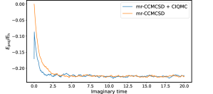
Figure 1: Convergence of $E_{\mathrm{proj}}$ in mr-CCMC calculations initialised from CASCIQMC or from the HF wavefunction for N₂ at $r_{\mathrm{NN}}=1.3$ Åin the STO-3G basis, using the standard mr-CCMC algorithm.

We describe a pair of approximations to the full mr-CCMC method which use the CASCIQMC wavefunction as a starting point. In the first frozen-reference mr-CCMC (fr-mr-CCMC) approach, no relaxation of the reference wavefunction from its CASCIQMC value is allowed. This is the same concept employed in TCC,Kinoshita, Hino, and Bartlett (2005) although the full cluster expansion of the CAS wavefunction is preserved, rather than maintaining only the $\hat{T}_{1}$ and $\hat{T}_{2}$ terms. This can be achieved by only permitting death and spawning into the external space. A second approach, referred to as relaxed-reference (rr-mr-CCMC) allows relaxation of the reference space in response to the external clusters, but not to internal changes. This corresponds to allowing spawning into the reference space from the external space, but no internal-internal spawning.

III.2 Combining CIQMC and CCMC populations

Implementing any of the approaches discussed above involves a mixture of CIQMC and CCMC amplitudes, which will have different numerical values for an arbitrary determinant, when used to describe the same wavefunction. The simplest approach is to translate the CASCIQMC wavefunction into a CCMC form, by a process known as cluster analysis. Alternatively, the mixed CI-CC representation can be maintained and the selection algorithm altered to account for this.

III.2.1 Cluster analysis

Consider expressing a wavefunction in two equivalent ways:

$$\ket{\Psi}=(1+\hat{C})\ket{D_{0}}=e^{\hat{T}}\ket{D_{0}}.$$ (19)

Expanding each of these expressions gives

$$\ket{\Psi}=(1+\sum_{ia}c_{i}^{a}\hat{a}^{\dagger}\hat{i}+\sum_{ijab}c_{ij}^{ab}\hat{a}^{\dagger}\hat{b}^{\dagger}\hat{j}\hat{i}+...)\ket{D_{0}}$$ (20)

and

$$\ket{\Psi}=(1+\sum_{ia}t_{i}^{a}\hat{a}^{\dagger}\hat{i}+\sum_{ijab}(t_{ij}^{ab}-\frac{t_{i}^{a}t_{j}^{b}}{2!}+\frac{t_{i}^{b}t_{j}^{a}}{2!})\hat{a}^{\dagger}\hat{b}^{\dagger}\hat{j}\hat{i}+...)\ket{D_{0}}$$ (21)

respectively. Equating each term from the sums gives equations of the form

$$\begin{split}&c_{i}^{a}=t_{i}^{a}\\ &c_{ij}^{ab}=t_{ij}^{ab}-\frac{t_{i}^{a}t_{j}^{b}}{2}+\frac{t_{i}^{b}t_{j}^{a}}{2}\\ &\mathrm{etc.}\end{split}$$ (22)

Given an intermediately normalised CI wavefunction, these equations can be used to construct the corresponding CC expansion. In the context of QMC methods, the normalisation of the wavefunction must be accounted for. The easiest way to maintain this consistently is to divide the obtained CIQMC populations by $N_{0}$, perform the cluster analysis and re-multiply the resulting CC amplitudes by the same $N_{0}$. This also provides an easy means to modify the normalisation between the CIQMC and mr-CCMC calculations if desirable.

III.2.2 Mixed CI-CC sampling

If a CI wavefunction is preserved in the reference space, the Ansatz has the form

$$\ket{\Psi}=e^{\hat{T}_{\mathrm{ext}}}(1+\hat{C}_{\mathrm{int}})\ket{D_{0}}.$$ (23)

Given the form of this expansion, each cluster of excitors selected in CCMC as described in section II.2 must contain a contribution from up to one internal excitation operator, as $\hat{C}_{\mathrm{int}}$ is a sum of these. Additionally, as the excitation operators commute and the internal and external operator pools are distinct, one can choose to always apply the internal excitation first when working out the determinant corresponding to a particular CCMC cluster selection. It is therefore possible to sample this expansion in the following way:

1. Select a cluster size $s$ with some probability $p_{s}$. This can be done with any of the available selection schemes.

2. Select a reference with probability

   $$p(r)=\frac{\lvert N_{r}\rvert}{\sum_{i\in\mathrm{refs}}\lvert N_{i}\rvert}.$$ (24)

3. If the selected reference is $\ket{D_{0}}$, then select $s$ excitors with

   $$p(e|s)=s!\prod_{i=1}^{s}\frac{|N_{i}|}{N_{\mathrm{ex}}},$$ (25)

   where $N_{\mathrm{ex}}$ is now the total population on non-reference excitors. If the selected reference is not $\ket{D_{0}}$, then $s-1$ excitors are selected with

   $$p(e|s)=(s-1)!\prod_{i=1}^{s-1}\frac{|N_{i}|}{N_{\mathrm{ex}}}.$$ (26)

The rest of the algorithm is largely left unchanged, although care must be taken to account for potential sign differences between $\ket{D_{ij...}^{ab...}}$ and $\hat{a}_{ij...}^{ab...}\ket{D_{0}}$.

IV Approximate mr-CCMC

IV.1 Perturbation theory treatment

We characterise the proposed approximate mr-CCMC approaches mathematically using small example systems and the framework of perturbation theory (PT). This allows us to predict some of the properties and limitations of these methods.

Consider first a system with two reference determinants, $\ket{D_{0}}$ and $\ket{D_{1}}$, and one external determinant, $\ket{D_{2}}$. The CIQMC equations in the reference space are given by

$$\begin{split}\braket{D_{0}}{\hat{H}-S_{\mathrm{ref}}}{\Psi}=0\\ \braket{D_{1}}{\hat{H}-S_{\mathrm{ref}}}{\Psi}=0,\end{split}$$ (27)

where we have substituted the shift $S_{\mathrm{ref}}$ for the unknown ground state energy of the reference space. These expand to

$$\begin{split}(H_{00}-S_{\mathrm{ref}})c_{0}+H_{01}c_{1}=0\\ (H_{11}-S_{\mathrm{ref}})c_{1}+H_{10}c_{0}=0.\end{split}$$ (28)

Setting $H_{00}=0$ and $c_{0}=1$ gives

$$S_{\mathrm{ref}}=\frac{H_{11}\pm\sqrt{H_{11}^{2}+4H_{01}^{2}}}{2}\ \ \mathrm{and}\ \ c_{1}=\frac{S_{\mathrm{ref}}}{H_{01}}.$$ (29)

Outside the reference space, the cluster amplitude equation is

$$(H_{22}-S)t_{2}+H_{20}c_{0}+H_{21}c_{1}=0,$$ (30)

with the shift $S$ now replaces the overall ground state energy, which should in general be different from $S_{\mathrm{ref}}$ as it takes into account external wavefunction contributions. This gives

$$t_{2}=\frac{H_{20}+H_{21}c_{1}}{S-H_{22}}.$$ (31)

We observe that, for fixed $c_{0}$ and $c_{1}$ and any value of $S$ there is a value of $t_{2}$ that obeys eq. 31. This is equivalent to each value of $S$ generating a different wavefunction. Therefore, when the reference space wavefunction is frozen, $S$ can no longer be freely used as a population control parameter and, instead, a physically justified value of $S$ is required. Two obvious options are available: $S=S_{\mathrm{ref}}$ and $S=E_{\mathrm{proj}}$, the use of which allows us to relate the resulting equations to terms in Rayleigh–SchrödingerStrutt, Baron Rayleigh (1894); Schrödinger (1926) (RS) and Brillouin–WignerBrillouin (1932); Wigner (1935) (BW) perturbation theory (PT) respectively.

As an example, consider a system with two references and two external excitors. We can set up a PT problem with $\hat{H}=\hat{H}_{0}+\hat{V}$ where the corresponding matrices are

$$\mathbf{H}_{0}=\begin{pmatrix}0&H_{01}&0&0\\ H_{10}&H_{11}&0&0\\ 0&0&H_{22}&0\\ 0&0&0&H_{33}\end{pmatrix}$$ (32)

$$\mathbf{V}=\begin{pmatrix}0&0&H_{02}&H_{03}\\ 0&0&H_{12}&H_{13}\\ H_{20}&H_{21}&0&H_{23}\\ H_{30}&H_{31}&H_{32}&0\end{pmatrix},$$ (33)

where $H_{\mu\nu}=\braket{D_{\mu}}{\hat{H}}{D_{\nu}}$. Diagonalising the reference Hamiltonian gives a set of zeroth-order wavefunctions,

$$\begin{split}&\ket{\phi_{0}}=c_{0}\ket{D_{0}}+c_{1}\ket{D_{1}}\\ &\ket{\phi_{1}}=c_{1}\ket{D_{0}}-c_{0}\ket{D_{1}}\\ &\ket{\phi_{2}}=\ket{D_{2}}\\ &\ket{\phi_{3}}=\ket{D_{3}}.\end{split}$$ (34)

At the first order of RSPT, the energy correction and the first order wavefunction contributions to $\ket{\Psi^{(1)}}=\sum_{\mu}a_{\mu}^{(1)}\ket{\phi_{\mu}}$ are given by:

$$E^{(1)}=\braket{\phi_{0}}{\hat{V}}{\phi_{0}}=0$$ (35)

$$a_{1}^{(1)}=0,$$ (36)

$$a_{2}^{(1)}=\frac{H_{20}c_{0}+H_{21}c_{1}}{E_{0}^{(0)}-H_{22}},$$ (37)

$$a_{3}^{(1)}=\frac{H_{30}c_{0}+H_{31}c_{1}}{E_{0}^{(0)}-H_{33}}.$$ (38)

The second-order wavefunction contributions to $\ket{\Psi^{(2}}=\sum_{\mu}a_{\mu}^{(2)}\ket{\phi_{\mu}}$ are given by

$$a_{1}^{(2)}=\frac{a_{2}^{(1)}\widetilde{H}_{21}+a_{3}^{(1)}\widetilde{H}_{31}}{E_{0}^{(0)}-E_{1}^{(0)}},$$ (39)

$$a_{2}^{(2)}=\frac{a_{3}^{(1)}H_{23}}{E_{0}^{(0)}-H_{22}},$$ (40)

$$a_{3}^{(2)}=\frac{a_{2}^{(1)}H_{32}}{E_{0}^{(0)}-H_{33}},$$ (41)

where $\widetilde{H}_{ij}=\braket{\phi_{i}}{\hat{H}}{\phi_{j}}$.

Note that the denominator in the equations above is the death term in QMC, if $S=E_{0}^{(0)}$. As FCIQMC gives the exact ground state energy in the reference space, this is equivalent to $S=S_{\mathrm{ref}}$. If one were to alternatively work through the above in a Brillouin–Wigner formalism, all appearances of $E_{0}^{(0)}$ in the denominator would be replaced by the total energy $E$. While this is not known a priori, QMC provides an estimate of it in the form of the instantaneous projected energy. Therefore, BWPT is related to our approach in the same way as described above, if $S=E_{\mathrm{proj}}$.

In this simple PT picture, the two approximations described in section III.1 correspond to selectively including some of the terms in Equations 36, 37, 38, 39, 40 and 41. If the initial CASCI wavefunction in the reference space is frozen one uses all the first-order terms and the purely external second-order terms $a_{2}^{(2)}$ and $a_{2}^{(3)}$. Adding the mixed internal-external second-order $a_{2}^{(1)}$ term corresponds to also allowing some relaxation of the reference space.

While these models are very simple, and notably fail to account for any of the added complexities of dealing with cluster amplitudes rather than a linear expansion, they do suggest some considerations when implementing these algorithms. We can consider a generic form of Equations 36, 37, 38, 39, 40 and 41, in which the denominators depend on an arbitrary parameter $S$ rather than $E_{0}^{(0)}$. These equations would have poles when $S$ is very close to one of the diagonal Hamiltonian elements outside the reference space, $H_{22}$ or $H_{33}$. This is relatively unlikely to be problematic for $S=E\approx E_{\mathrm{proj}}$, as the shift tracks the lowest eigenvalue, which should be lower than any diagonal Hamiltonian elements. There is a more significant risk of interacting with poles when $S=S_{\mathrm{ref}}=E_{0}^{(0)}$, as this value will in general be higher than the ground state and may be close to other Hamiltonian elements. We find that this is indeed a problem in the strongly correlated regimes of the systems considered here, for which $S_{\mathrm{ref}}$ is above the stability threshold for the equations.

When considering the additional term in rr-mr-CCMC (eq. 39), we observe that unsurprisingly any spawning into the reference space (given by ${a_{2}^{(1)}\widetilde{H}_{21}+a_{3}^{(1)}\widetilde{H}_{31}}$) must be accompanied by death in this space (given by $E_{0}^{(0)}-E_{1}^{(0)}$) to prevent uncontrolled population growth. Secondly, we note that all spawning towards and death in the reference space should occur onto the excited states of the reference Hamiltonian $\ket{\phi_{i}}$ rather than onto the reference determinants $\ket{D_{i}}$. If one is using CASCIQMC to find the ground state in the reference space, the wavefunctions and energies of these excited states are unknown. However, enforcing that any contribution be orthogonal to the CAS ground state is possible and sufficient for a viable propagator, as is discussed in section IV.2.2.

IV.2 Algorithmic Details

In all cases, an FCIQMC calculation is run in a CAS. This active space is then used as a reference space for an mr-CCMC calculation, with the population initialised to the FCIQMC values or a cluster expansion thereof. The constraints placed on the mr-CCMC calculation to obtain approximate solutions are given below.

IV.2.1 Frozen-reference mr-CCMC

The fr-mr-CCMC approach can be simply implemented by rejecting all spawning and death attempts in the reference space. The shift can then be fixed to a value or set to track the instantaneous projected energy. The idea of a population threshold is no longer relevant, so the shift should start varying or be set to its final value at the beginning of the mr-CCMC calculation. For simplicity, the CC form of the reference wavefunction is used in this case.

IV.2.2 Relaxed-reference mr-CCMC

The rr-mr-CCMC method could be implemented naïvely by allowing death within the reference space and all spawning attempts from determinants in the external space. As is shown later in LABEL:sec:na\"ive_erds, this implementation would not generate a correct propagator. Ideally, we would express the CAS Hilbert space in the eigenvector basis of the CAS Hamiltonian and allow each eigenvector to undergo death and spawning independently. This is not possible when starting from a CIQMC calculation, where only the lowest eigenvector is known. However, we can enforce that excitations and death within the reference space occur within the subspace orthogonal to the CIQMC ground state. This is more easily done by preserving the CI representation of the CAS wavefunction.

Consider a set of vectors $\{\ket{\Phi_{k}}\}$ which span the reference space, where $\ket{\Phi_{0}}$ is the CASCIQMC wavefunction and the others are an arbitrary set of orthogonal vectors spanning the rest of the space. Starting from eq. 5, for reference determinant $\ket{D_{\mu}}$, with the shift substituted for the energy and combining the spawning and death terms into one,

$$c_{\mu}(\tau+\Delta\tau)=c_{\mu}(\tau)-\Delta\tau\braket{D_{\mu}}{\hat{H}-S}{\Psi}$$ (42)

The identity operator can be resolved as

$$\hat{I}=\sum_{k=0}^{n_{\mathrm{ref}}-1}\ket{\Phi_{k}}\bra{\Phi_{k}}+\sum_{\nu=n_{\mathrm{ref}}}^{N}\ket{D_{\nu}}\bra{D_{\nu}}.$$ (43)

Introducing this on either side of the Hamiltonian in eq. 42 and noting that the reference determinant $\ket{D_{\mu}}$ is orthogonal to all non-reference determinants,

$$\begin{split}c_{\mu}(\tau+\Delta\tau)&=c_{\mu}(\tau)\\ &-\Delta\tau\big{(}\sum_{k,l}\braket{D_{\mu}}{\Phi_{k}}\braket{\Phi_{k}}{\hat{H}-S}{\Phi_{l}}\braket{\Phi_{l}}{\Psi}\\ &+\sum_{k,\nu}\braket{D_{\mu}}{\Phi_{k}}\braket{\Phi_{k}}{\hat{H}}{D_{\nu}}\braket{D_{\nu}}{\Psi}\big{)}.\end{split}$$ (44)

If internal spawning and death on the ground reference state is explicitly forbidden, this reduces to

$$\begin{split}c_{\mu}(\tau+\Delta\tau)&=c_{\mu}(\tau)\\ &-\Delta\tau\big{(}\sum_{k}\braket{D_{\mu}}{\Phi_{k}}\braket{\Phi_{k}}{\hat{H}-S}{\Phi_{k}}\braket{\Phi_{k}}{\Psi}\\ &+\sum_{k,\nu}\braket{D_{\mu}}{\Phi_{k}}\braket{\Phi_{k}}{\hat{H}}{D_{\mathbf{j}}}\braket{D_{\nu}}{\Psi}\big{)}.\end{split}$$ (45)

Monte Carlo Sampling this equation can be done in the following way:

1. For each Monte Carlo cycle, generate a random state within the reference space $\ket{\Phi_{r}}=\sum_{i\in\mathrm{ref}}c_{r\mu}\ket{D_{\mu}}$ orthogonal to $\ket{\Phi_{0}}$. Then compute $E_{r}=\braket{\Phi_{r}}{\hat{H}}{\Phi_{r}}$.

2. For each death attempt in the reference space, death probability on each reference determinant $D_{\mu}$ is proportional to $|E_{r}-S|N_{r}c_{r\mu}$, where $N_{r}=\braket{\Phi_{r}}{\Psi_{\mathrm{CC}}}$.

3. For each spawning attempt in the reference space, the spawning probability onto a determinant $D_{\mu}$ is proportional to $\braket{\Phi_{r}}{\hat{H}}{D_{\nu}}c_{r\mu}N_{\nu}$ where $D_{\nu}$ is the determinant spawning originates from and $N_{\nu}$ is its population.

IV.3 Shift in frozen-reference mr-CCMC

Two physically justified options for the shift in a frozen-reference mr-CCMC calculation have been identified: $S=S_{\mathrm{ref}}$ and $S=E_{\mathrm{proj,inst}}$, where $E_{\mathrm{proj,inst}}$ is the intantaneous projected energy. We investigate the effect of these choices on fr-mr-CCMC using the H₄ molecule in a square geometry and a minimal basis set,Jankowski and Paldus (1980) (see supplementary material for parameters) while varying the side-length $a$.

Owing to symmetry, this molecule has two degenerate frontier molecular orbitals, which lead to degenerate lowest-energy single-determinant wavefunctions $\ket{1^{\alpha}1^{\beta}2^{\alpha}3^{\beta}}$ and $\ket{1^{\alpha}1^{\beta}2^{\beta}3^{\alpha}}$. These can be used as references in 2r-CCMCSD, giving the energies shown in Table 1. Solving the CASCIQMC problem in the reference space and then using the fr-mr-CCMC algorithm with $S=E_{\mathrm{proj,inst}}$ gives very good agreement with the full results, however the same is not true for $S=E_{\mathrm{ref}}$ (see Table 1).

$r_{\mathrm{HH}}$	FCI $E$	2r-CCMCSD $S$	2r-CCMCSD $E_{\mathrm{proj}}$	fr-2r-CCMCSD $E_{\mathrm{proj}}$ ($S=E_{\mathrm{proj,inst}}$)	fr-2r-CCMCSD $E_{\mathrm{proj}}$ ($S=S_{\mathrm{ref}}$)
2.0	-0.08833198	-0.08838(4)	-0.08833(3)	-0.08844(2)	-0.0897(3)
2.5	-0.11429334	-0.11423(3)	-0.11424(4)	-0.11384(3)	-0.1189(4)
3.0	-0.14896567	-0.14891(2)	-0.14892(4)	-0.14883(4)	-0.1696(6)
5.0	-0.34077014	-0.34070(5)	-0.3408(1)	-0.34079(8)	-
7.0	-0.46322289	-0.46343(5)	-0.4637(2)	-0.4636(2)	-
9.0	-0.51183106	-0.51185(4)	-0.5117(1)	-0.5113(2)	-
11.0	-0.53447267	-0.53449(8)	-0.5345(1)	-0.5349(1)	-
13.0	-0.54864903	-0.54858(4)	-0.5487(1)	-0.5483(1)	-

Table 1: Values of the shift $S$ and the projected energy $E_{\mathrm{proj}}$ of H₄ computed using 2r-CCMC and its frozen-reference approximation.

When the shift is set to equal $S_{\mathrm{ref}}$, the calculations only converge for relatively short bond lengths, beyond which the population starts growing exponentially.

We prove in section IV.1 that, for a particular model problem, there is a solution for any fixed value of the shift. We expect this to be the case in general for this type of ansatz and investigate this numerically here. A range of such values is considered in Fig. 2, and the CIQMC and mr-CCMC equations are propagated deterministically to eliminate any possible uncertainty due to noise. As can be seen, the correct value of the projected energy can only be achieved in the fixed-shift regime when $S=E_{\mathrm{proj}}$.

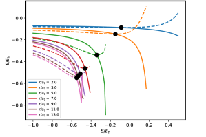
Figure 2: Converged $E_{\mathrm{proj}}$ (solid) and variational estimator $\braket{E}$ (dashed) for fr-2r-CCMCSD calculations for H₄ as a function of set shifts, at different values of $r_{\mathrm{HH}}$. Black circles corresponding to the correct value of $E_{\mathrm{proj}}$ lie on the $E=S$ line.

While this point is unremarkable on the projected energy surface, it corresponds to a minimum in the attained variational energy, as well as a crossing point between the two surfaces. Therefore, the $S=E_{\mathrm{proj,inst}}$ approach corresponds to a variational optimisation of the shift parameter.

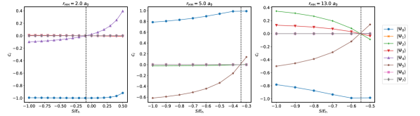
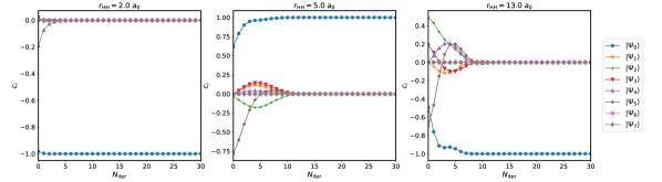
Figure 3: Top: The projection of the final solution of the fr-2r-CCMCSD equations onto the FCI eigenfunctions for various set shifts at H-H distances of 2.0, 5.0 and 13.0 $a_{0}$. Bottom: The projection of the fr-2r-CCMCSD solution with $S=E_{\mathrm{proj,inst}}$ onto the FCI eigenfunctions as a function of the number of imaginary time steps.

In this case, the true value of the projected energy is always within the stability threshold of the calculation, although the margin decreases as correlation increases.

We further examine the wavefunctions obtained in the fixed shift regime by comparing their projections onto the FCI eigenfunctions. In all cases considered in Fig. 3, the propagation only converges onto a single eigenstate at $S=E_{\mathrm{proj}}$. In comparison, the $S=E_{\mathrm{proj,inst}}$ method starts in a mix of states, goes through an intermediate period where contributions from multiple excited states exist and quickly settles onto a single eigenstate. Convergence onto a single eigenstate is possible in this case because frozen-reference 2r-CCMC happens to be equivalent to FCI for H4, but this is not guaranteed in general.

These considerations suggest the $S=E_{\mathrm{proj,inst}}$ propagator as the sensible choice for a fr-mr-CCMC approach, so we will focus on this for further numerical results.

IV.4 The relaxed-reference mr-CCMC propagator

In general, we expect differences between the CASCI wavefunction and the projection of the true ground state wavefunction onto the CAS. This discrepancy is responsible for systematic errors in TCC,Faulstich et al. (2019) which we expect to appear in fr-mr-CCMC as well. Therefore we expect methods which allow some relaxation of the CAS coefficients in the presence of the CCMC wavefunction to give improved estimates. While not necessary for H₄, a correct propagator which allows external spawning into the reference space should not negatively impact the quality of the result. As in conventional mr-CCMC, calculations set up in this way have the benefit of a well-defined shift, independent of $E_{\mathrm{proj}}$, which can be used for population control. However, the results of a naïve implementation of the rr-mr-CCMC method, which allows independent spawning and death onto reference determinants, are very poor. The propagator fails to select a single eigenstate regardless of bond length (see Fig. 4).

The failures become increasingly pathological for more correlated geometries. This can be corrected by spawning onto vectors perpendicular to the CASCI wavefunction, as discussed in section IV.2.2 (see Fig. 5). The random orthogonal vector propagator is equivalent to the eigenvector-based propagator in this case as there is only one vector orthogonal to the ground state in the reference space.

In order to meaningfully assess the quality of the random orthogonal vector propagator, we turn to the Hubbard model,Hubbard (1963) used to describe conducting and insulating behaviour in extended lattices. Consider a lattice with sites $r$, each of which has a single spatial orbital centred on it. The Hamiltonian for this system is given by

$$\hat{H}=-t\sum_{\braket{r,r^{\prime}},\sigma}\hat{c}_{r,\sigma}^{\dagger}\hat{c}_{r^{\prime},\sigma}+U\sum_{r}\hat{n}_{r,\uparrow}\hat{n}_{r,\downarrow}$$ (46)

where $\hat{c}_{r,\sigma}^{\dagger}$ and $\hat{c}_{r,\sigma}$ are creation and annihilation operators at site $r$ and $\hat{n}_{r,\sigma}$ is the corresponding number operator. The pair $\braket{r,r^{\prime}}$ ranges over adjacent sites.

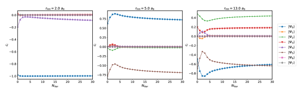
Figure 4: Projections onto the FCI eigenfunctions of the naïvely propagated H₄ rr-2r-CCMCSD wavefunction as a function of imaginary time at H-H distances of 2.0, 5.0 and 13.0 $a_{0}$

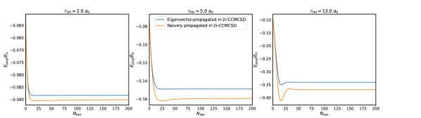
Figure 5: Projected energy of the H₄ rr-2r-CCMCSD wavefunction as a function of imaginary time at H-H distances of 2.0, 5.0 and 13.0 $a_{0}$. Naive propagation leads to an overestimate of the correlation energy.

The hopping integral $t$ and the on-site interaction integral $U$ are free parameters of the model, whose behaviour is controlled by the $U/t$ ratio, with higher values corresponding to more strongly correlated systems.

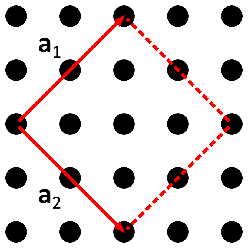
Figure 6: Graphic representation of the 8-site Hubbard lattice (left) and the corresponding half-filled MO diagram (right).

For our investigation we consider the 2D half-filled 8-site Hubbard model described in Fig. 6, using momentum space orbitals which represent the symmetry conserved HF solutions. Its ground state falls in the $\Gamma$-symmetry sector with momentum $\mathbf{k}=(0,0)$. In this case, the (6,6)-CASCI ground state corresponds exactly to the CAS contribution to the true ground state. Moving away from the $\Gamma$ point to the $\mathbf{k}=(0,1)$ space, two CASCI eigenfunctions contribute to the true ground state. Fig. 7 gives the energy obtained by deterministic propagation of FCIQMC as well as single- and multireference CCMC. mr-CCMCSD and rr-mr-CCMCSD with random or true eigenvalue reference dynamics agree well with each other, while fr-mr-CCMCSD is now slightly above them in energy — see table 2.

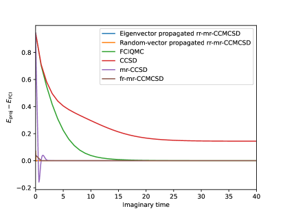
Figure 7: Projected energy as a function of imaginary time in the 8-site Hubbard model with $U=t$ at $\mathbf{k}=(0,1)$. The eigenvector propagated rr-mr-CCMCSD line (blue) is obscured by the random-vector propagated rr-mr-CCMCSD line (orange).

Method	Projected energy
CCSD	-0.806154
48r-CCSD	-0.949993
fr-48r-CCSD	-0.949987
rr-48r-CCSD (eigenvector propagation)	-0.949993
rr-48r-CCSD (random vector propagation)	-0.949998
FCIQMC	-0.950210

Table 2: Converged energies for the 8-site Hubbard model with $U$ = $t$ at $\mathbf{k}=(0,1)$, using different mr-CCMC approaches propagated deterministically.

IV.5 Stochastic frozen-reference and relaxed-reference mr-CCMC results.

The previous sections have used deterministic propagations of the mr-CCMC wavefunction and its partially relaxed approximations to draw conclusions about these approaches, which we reiterate here. In order to get physically meaningful results out of fr-mr-CCMC, the shift must be allowed to exactly follow the projected energy. For rr-mr-CCMC, naïve propagation is not appropriate, but using random vectors orthogonal to the CASCI ground state as a basis for the reference space provides a promising alternative. Making use of these observations, we move to a true stochastic propagation of the wavefunction and investigate the quality of these approximations in the presence of random noise for a range of Li-based systems, which, unlike Hubbard models, have a well-defined core, making it easier to define reference spaces.

IV.5.1 A highly multiconfigurational species

We begin by looking at the LiH3 molecule in the STO-3G basis. This toy system is designed to have many large contributions to the ground state wavefunction, dominated by single excitations of the HF wavefunction. The HF wavefunction itself makes a negligible contribution to the ground state, making this system particularly challenging for single-reference methods and in this case single-reference CCMCSD fails to converge. Using a (4,4)-CAS as a reference space for mr-CCMCSD leads to the results shown in table 3.

Method	Projected energy
36r-CCMCSD	-0.2789(6)
fr-36r-CCMCSD	-0.27566(4)
rr-36r-CCMCSD	-0.2760(1)
FCIQMC	-0.2795(3)
FCI	-0.279161

Table 3: LiH₃ energies from different mr-CCMC approaches, together with FCIQMC and FCI benchmarks.

In this case, while full 36r-CCMCSD is within one standard deviation of the FCI value, the approximate methods are not as accurate, although rr-mr-CCMCSD provides an improvement over the frozen-reference approach. However, the approximations are not without benefits. As can be seen in fig. 8, using either the frozen- or relaxed-reference approach leads to faster convergence and significantly lower noise than the full mr-CCMC or the FCIQMC calculations.

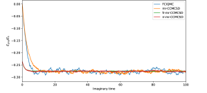
Figure 8: Convergence of $E_{\mathrm{proj}}$ with imaginary time for FCIQMC, mr-CCMC and the partially relaxed approximations in LiH₃. Approximate methods converge faster and lead to lower noise.

While the noise is not problematic in this system, CCMC calculations are at times metastable with respect to non-physical solutions with large oscillations likely to push them towards these undesirable alternate solutions. Noise reduction is therefore a valuable property.

IV.5.2 Li structures

Finally, we consider a set of small Li clusters, using reduced basis sets in which each Li atom has only two or three $s$ orbitals. We investigate 4- and 6-membered Li rings and chains over a wide range of Li-Li bond lengths. Near equilibrium, Li chains are well-behaved single-reference systems, as is the 6-membered ring. The 4-membered Li ring has significant multireference character at all geometries due to the presence of a partially occupied degenerate pair of spatial orbitals. Binding curves computed with FCI(QMC), mr-CCMCSD and partially relaxed approximations thereof are given in fig. 9 and 10. For the smaller of the two basis sets, CCMCSD results start diverging from the FCI energy at large Li-Li separations. In comparison, mr-CCMCSD and its approximations generally maintain excellent agreement with the exact results, with the notable exception of rr-mr-CCSD in the 4-membered Li ring, which has noticeable errors (up to 5$\mathrm{m}E_{\mathrm{h}}$) across the entire binding curve. rr-mr-CCSD also shows a number of outliers across the other binding curves, converging to the wrong energy values with significantly larger error bars than neighbouring values. For the Li₄ ring, the mr-CCSD method is difficult to converge around $r_{\mathrm{LiLi}}=1.9$Å, but both the frozen- and relaxed-reference approaches converge without issue over the entire binding curve.

For the larger basis set, both CCSD and mr-CCSD are almost exact for the Li4 chain in the range of basis states considered. However, both the frozen- and relaxed-reference approximations now have noticeable systematic errors. In contrast, for the Li4 ring, where CCMCSD diverges from FCI as $r_{\mathrm{LiLi}}$ increases, approximate mr-CCMCSD methods perform significantly better than the single-reference approach and converge over the whole range of bond-lengths, unlike the unapproximated mr-CCMCSD method.

V Conclusions

Using the reference CASCIQMC wavefunction as a starting point, we develop two approximations to the mr-CCMC method. Frozen-reference mr-CCMC keeps the reference wavefunction fixed to its initial

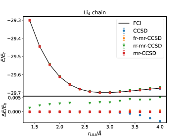
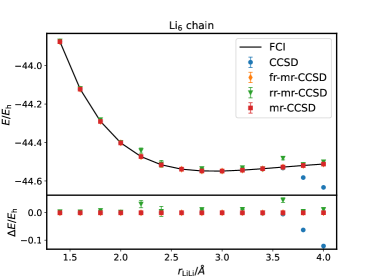
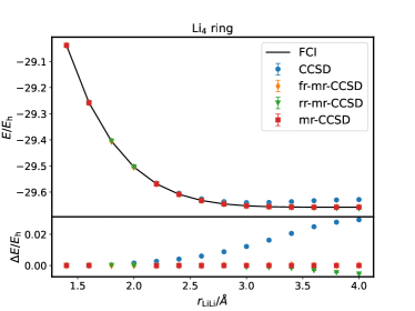
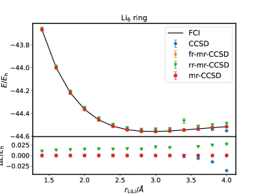
Figure 9: Binding curves and energy errors computed with mr-CCMC, fr-mr-CCMC and rr-mr-CCMC for the Li₄ chain (top left), Li₄ ring (bottom left), Li₆ chain (top right) and Li₆ ring (bottom right) with two $s$ orbitals per atom. fr-mr-CCMCSD agrees with the exact mr-CCMCSD calculation in all cases, but the rr-mr-CCMCSD approach displays a systematic error in the Li₄ chain and Li₆ ring, as well as generating a outliers in the energy curves of other systems.

CASCIQMC value, while relaxed-reference mr-CCMC only allows spawning onto reference determinants from the external space. These two methods are shown to have different propagation requirements from the original algorithm.

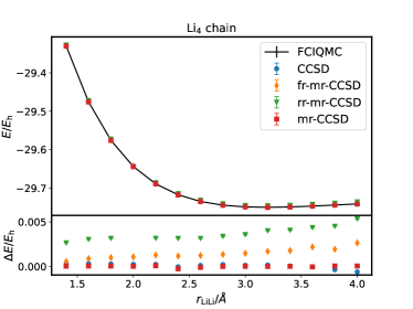
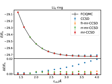
Figure 10: Binding curves and energy errors computed with mr-CCMC, fr-mr-CCMC and rr-mr-CCMC for the Li₄ chain (left), Li₄ ring (right) with 3 $s$ orbitals per atom. FCI benchmark is obtained from FCIQMC. For the ring structure, fr- and rr-mr-CCMC significantly outperform single-reference CCSD, but no longer agree perfectly with mr-CCMCSD. For the chain, CCMCSD itself is almost exact in the range of bondlengths studies, but the fr- and rr-mr-CCMC both now exhibit noticeable errors.

In fr-mr-CCMC, maintaining a steady-state population can no longer be used as a condition to find the shift as a wide range of values of $S$ give rise to stable populations. In order to get physically meaningful results, the shift is constrained to track the instantaneous projected energy, leading to the loss of one of the independent energy estimators from a conventional QMC calculation.

In rr-mr-CCMC, naïvely spawning onto determinants in the reference space leads to a propagator that fails to converge to the ground state of the system even when the method is formally exact and is found to overestimate the correlation energy. This can be mitigated by constraining spawns to the space orthogonal to the CASCIQMC ground state. This approach is applied successfully to the Hubbard model, where the additional relaxation leads to better energy estimates than the frozen-reference approximation. However, the fully stochastic implementation displays systematic errors when applied to a Li₄ chain and shows a propensity for spuriously converging to non-physical solutions in other Li structures as well. As noted in the deterministic examples, propagation that is not fully orthogonal to the ground CASCI wavefunction leads to unphysical rr-mrCC energies. rr-mr-CCMC calculations are based on a stochastic snapshot of the CASCI wavefunction which, particularly for relatively small walker numbers, is unlikely to be perfectly aligned with the true CASCI ground state, so the random states generated during the propagation will not be exactly orthogonal to the ground state either, leading to errors in the rr-mr-CCMC propagation.

Generally, these approximations are found to converge faster than the exact mr-CCMC method, as expected since they are initialised in a multireference state, rather than with the HF determinant. While all examples in this paper use a CAS reference, this is not a requirement for any of the methods presented. Stochastic noise in the calculations is also reduced relative to the exact approach, which allows the approximations to converge in regimes where mr-CCMC is ill-behaved. For the systems we have studied, allowing partial relaxation of the reference wavefunction does not normally lead to substantial accuracy gains and in some cases the method is more error-prone than the simpler frozen-reference a pproximation. In cases where there is a significant difference between single- and multireference results, this approximation generally significantly outperforms the single-reference approach, presenting a viable alternative when exact mr-CCMC calculations would be unstable or prohibitively expensive.

Supplementary Material

See supplementary material for the basis set used for H₄ .

Data Availability Statement

The data that support the findings of this study are openly available in the Apollo University of Cambridge Repository at http://doi.org/10.17863/CAM.93604, reference number 6321755.

Author Declarations

The authors have no conflicts to disclose.

References

- Raghavachari et al. (1989) K. Raghavachari, G. W. Trucks, J. A. Pople, and M. Head-Gordon, “A fifth-order perturbation comparison of electron correlation theories,” Chem. Phys. Lett. 157, 479 (1989).
- Andersson et al. (1990) K. Andersson, P. A. Malmqvist, B. O. Roos, A. J. Sadlej, and K. Wolinski, “Second-order perturbation theory with a CASSCF reference function,” J. Phys. Chem. 94, 5483 (1990).
- Angeli et al. (2001) C. Angeli, R. Cimiraglia, S. Evangelisti, T. Leininger, and J.-P. Malrieu, “Introduction of n-electron valence states for multireference perturbation theory,” J. Chem. Phys. 114, 10252 (2001).
- Angeli, Cimiraglia, and Malrieu (2001) C. Angeli, R. Cimiraglia, and J.-P. Malrieu, “N-electron valence state perturbation theory: A fast implementation of the strongly contracted variant,” Chem. Phys. Lett. 350, 297 (2001).
- Angeli, Cimiraglia, and Malrieu (2002) C. Angeli, R. Cimiraglia, and J.-P. Malrieu, “N-electron valence state perturbation theory: A spinless formulation and an efficient implementation of the strongly contracted and of the partially contracted variants,” J. Chem. Phys. 117, 9138 (2002).
- Lyakh et al. (2011) D. I. Lyakh, M. Musiał, V. F. Lotrich, and R. J. Bartlett, “Multireference Nature of Chemistry: The Coupled-Cluster View,” Chem. Rev. 112, 182 (2011).
- Kaldor (1988) U. Kaldor, “Intruder states and incomplete model spaces in multireference coupled-cluster theory: The 2 states of be,” Phys. Rev. A 38, 6013 (1988).
- Paldus et al. (1993) J. Paldus, P. Piecuch, L. Pylypow, and B. Jeziorski, “Application of hilbert-space coupled-cluster theory to simple (h2)2 model systems: Planar models,” Phys. Rev. A 47, 2738 (1993).
- Jankowski and Malinowski (1994) K. Jankowski and P. Malinowski, “A valence-universal coupled-cluster single-and double-excitations method for atoms. iii. solvability problems in the presence of intruder states,” J. Phys. B 27, 1287 (1994).
- Piecuch and Paldus (1994) P. Piecuch and J. Paldus, “Application of hilbert-space coupled-cluster theory to simple ( model systems. ii. nonplanar models,” Phys. Rev. A 49, 3479 (1994).
- Paldus (2017) J. Paldus, “Externally and internally corrected coupled cluster approaches: An overview,” J. Math. Chem. 55, 477 (2017).
- Schriber and Evangelista (2016) J. B. Schriber and F. A. Evangelista, “Communication: An adaptive configuration interaction approach for strongly correlated electrons with tunable accuracy,” J. Chem. Phys. 144, 161106 (2016).
- Deustua, Shen, and Piecuch (2017) J. E. Deustua, J. Shen, and P. Piecuch, “Converging High-Level Coupled-Cluster Energetics by Monte Carlo Sampling and Moment Expansions,” Phys. Rev. Lett. 119, 223003 (2017).
- Deustua et al. (2018) J. E. Deustua, I. Magoulas, J. Shen, and P. Piecuch, “Communication: Approaching exact quantum chemistry by cluster analysis of full configuration interaction quantum Monte Carlo wave functions,” J. Chem. Phys. 149, 151101 (2018).
- Deustua, Shen, and Piecuch (2021) J. E. Deustua, J. Shen, and P. Piecuch, “High-level coupled-cluster energetics by Monte Carlo sampling and moment expansions: Further details and comparisons,” J. Chem. Phys. 154, 124103 (2021).
- Kinoshita, Hino, and Bartlett (2005) T. Kinoshita, O. Hino, and R. J. Bartlett, “Coupled-cluster method tailored by configuration interaction,” J. Chem. Phys. 123, 074106 (2005).
- Mörchen, Freitag, and Reiher (2020) M. Mörchen, L. Freitag, and M. Reiher, “Tailored coupled cluster theory in varying correlation regimes,” J. Chem. Phys. 153, 244113 (2020).
- Vitale, Alavi, and Kats (2020) E. Vitale, A. Alavi, and D. Kats, “FCIQMC-Tailored Distinguishable Cluster Approach,” J. Chem. Theory Comput. 16, 5621 (2020).
- Veis et al. (2016) L. Veis, A. Antalìk, J. Brabec, F. Neese, O. Legeza, and J. Pittner, “Coupled cluster method with single and double excitations tailored by matrix product state wave functions,” J. Phys. Chem. Lett. 7, 4072 (2016).
- Booth, Thom, and Alavi (2009) G. H. Booth, A. J. W. Thom, and A. Alavi, “Fermion Monte Carlo without fixed nodes: A game of life, death, and annihilation in Slater determinant space,” J. Chem. Phys. 131, 054106 (2009).
- Thom (2010) A. J. W. Thom, “Stochastic coupled cluster theory,” Phys. Rev. Lett. 105, 263004 (2010).
- Neufeld and Thom (2017) V. A. Neufeld and A. J. W. Thom, “A study of the dense uniform electron gas with high orders of coupled cluster,” J. Chem. Phys. 147, 194105 (2017).
- Filip, Scott, and Thom (2019) M.-A. Filip, C. J. C. Scott, and A. J. W. Thom, “Multireference stochastic coupled cluster,” J. Chem. Theory Comput. 15, 6625 (2019).
- Ichibha et al. (2022) T. Ichibha, V. A. Neufeld, K. Hongo, R. Maezono, and A. J. W. Thom, “Making the most of data: Quantum monte carlo postanalysis revisited,” Phys. Rev. E 105, 045313 (2022).
- Vigor et al. (2015) W. A. Vigor, J. S. Spencer, M. J. Bearpark, and A. J. W. Thom, “Minimising biases in full configuration interaction quantum monte carlo,” J. Chem. Phys. 142, 104101 (2015).
- Franklin et al. (2016) R. S. Franklin, J. S. Spencer, A. Zoccante, and A. J. W. Thom, “Linked coupled cluster Monte Carlo,” J. Chem. Phys. 144, 044111 (2016).
- Spencer and Thom (2016) J. S. Spencer and A. J. W. Thom, “Developments in stochastic coupled cluster theory: The initiator approximation and application to the uniform electron gas,” J. Chem. Phys. 144, 084108 (2016).
- Neufeld and Thom (2019) V. A. Neufeld and A. J. W. Thom, “Exciting determinants in quantum monte carlo: Loading the dice with fast, low-memory weights,” J. Chem. Theory Comput. 15, 127 (2019).
- Spencer et al. (2018) J. S. Spencer, V. A. Neufeld, W. A. Vigor, R. S. T. Franklin, and A. J. W. Thom, “Large scale parallelization in stochastic coupled cluster,” J. Chem. Phys. 149, 204103 (2018).
- Scott and Thom (2017) C. J. C. Scott and A. J. W. Thom, “Stochastic coupled cluster theory: Efficient sampling of the coupled cluster expansion,” J. Chem. Phys. 1471, 124105 (2017).
- Oliphant and Adamowicz (1991) N. Oliphant and L. Adamowicz, “Multireference Method Using a Single-reference Formalism,” J. Chem. Phys. 94, 1229 (1991).
- Oliphant and Adamowicz (1992) N. Oliphant and L. Adamowicz, “The implementation of the multireference coupled-cluster method based on the single-reference formalism,” J. Chem. Phys. 96, 4282 (1992).
- Piecuch, Oliphant, and Adamowicz (1993) P. Piecuch, N. Oliphant, and L. Adamowicz, “A state-selective multireference coupled-cluster theory employing the single-reference formalism,” J. Chem. Phys. 99, 1875 (1993).
- Piecuch and Adamowicz (1994) P. Piecuch and L. Adamowicz, “State-selective multireference coupled-cluster theory employing the single-reference formalism: Implementation and application to the H8 model system,” J. Chem. Phys 100, 5792 (1994).
- Jeziorski and Monkhorst (1981) B. Jeziorski and H. J. Monkhorst, “Coupled-cluster method for multideterminantal reference states,” Phys. Rev. A 24, 1668 (1981).
- Mahapatra, Datta, and Mukherjee (1998) U. S. Mahapatra, B. Datta, and D. Mukherjee, “A state-specific multi-reference coupled cluster formalism with,” Mol. Phys. 94, 157 (1998).
- Mahapatra, Datta, and Mukherjee (1999) U. S. Mahapatra, B. Datta, and D. Mukherjee, “A size-consistent state-specific multireference coupled cluster theory: Formal developments and molecular applications,” J. Chem. Phys. 110, 6171 (1999).
- Adamowicz, Piecuch, and Ghose (1998) L. Adamowicz, P. Piecuch, and K. B. Ghose, “The state-selective coupled cluster method for quasi-degenerate electronic states,” Mol. Phys. 94, 225 (1998).
- Ivanov and Adamowicz (2000) V. V. Ivanov and L. Adamowicz, “Casccd: Coupled-cluster method with double excitations and the cas reference,” J. Chem. Phys. 112, 9258 (2000).
- Ivanov, Lyakh, and Adamowicz (2009) V. V. Ivanov, D. I. Lyakh, and L. Adamowicz, “Multireference state-specific coupled-cluster methods. state-of-the-art and perspectives,” Phys. Chem. Chem. Phys. 11, 2355 (2009).
- Strutt, Baron Rayleigh (1894) J. W. Strutt, Baron Rayleigh, The Theory of Sound (Macmillan, London, 1894).
- Schrödinger (1926) E. Schrödinger, “Quantisierung als eigenwertproblem,” Ann. Phys. 80, 437 (1926).
- Brillouin (1932) L. Brillouin, “Les problèmes de perturbations et les champs self-consistents,” J. Phys. Radium 3, 373 (1932).
- Wigner (1935) E. Wigner, “On a modification of the rayleigh–schrodinger perturbation theory,” Math. Naturwiss. Anz. Ungar. Akad. Wiss. 53, 477 (1935).
- Jankowski and Paldus (1980) K. Jankowski and J. Paldus, “Applicability of coupled-pair theories to quasidegenerate electronic states: A model study,” Int. J. Quantum Chem. 18, 1243 (1980).
- Faulstich et al. (2019) F. M. Faulstich, A. Laestadius, O. Legeza, R. Schneider, and S. Kvaal, “Analysis of the tailored coupled-cluster method in quantum chemistry,” SIAM J. Numer. Anal. 57, 2579 (2019).
- Hubbard (1963) J. Hubbard, “Electron correlations in narrow energy bands,” Proc. R. Soc. A 276, 238 (1963).
- Note (1) A low-symmetry molecular geometry is used — Li at and H atoms at , and — and orbitals are obtained from an SCF calculation with an exchange functional that is 10% Slater–Dirac exchangeDirac (1930) and 90% Hartree–Fock exchange.
- Dirac (1930) P. A. M. Dirac, “Note on exchange phenomena in the thomas atom,” P. Camb. Philos. Soc 26, 376 (1930).