Invariants for neural automata

Abstract.

Computational modeling of neurodynamical systems often deploys neural networks and symbolic dynamics. One particular way for combining these approaches within a framework called vector symbolic architectures leads to neural automata. An interesting research direction we have pursued under this framework has been to consider mapping symbolic dynamics (e.g. performed by Turing machines) onto neurodynamics, represented as neural automata. This representation theory, enables us to ask questions, such as, how does the brain implement Turing computations. Specifically, in this representation theory, neural automata result from the assignment of symbols and symbol strings to numbers, known as Gödel encoding. Under this assignment symbolic computation becomes represented by trajectories of state vectors in a real phase space, that allows for statistical correlation analyses with real-world measurements and experimental data. However, these assignments are usually completely arbitrary. Hence, it makes sense to address the problem question of, which aspects of the dynamics observed under such a representation is intrinsic to the dynamics and which are not. In this study, we develop a formally rigorous mathematical framework for the investigation of symmetries and invariants of neural automata under different encodings. As a central concept we define patterns of equality for such systems. We consider different macroscopic observables, such as the mean activation level of the neural network, and ask for their invariance properties. Our main result shows that only step functions that are defined over those patterns of equality are invariant under symbolic recodings, while the mean activation, e.g., is not. Our work could be of substantial importance for related regression studies of real-world measurements with neurosymbolic processors for avoiding confounding results that are dependant on a particular encoding and not intrinsic to the dynamics.

1. Introduction

Computational cognitive neurodynamics deals to a large extent with statistical modeling and regression analyses between behavioral and neurophysiological observables on the one hand and neurocomputational models of cognitive processes on the other hand (Gazzaniga et al 2002, Rabinovich et al 2012). Examples for experimentally measurable observables are response times (RT), eye-movements (EM), event-related brain potentials (ERP) in the domain of electroencephalography (EEG), event-related magnetic fields (ERF) in the domain of magnetoencephalography (MEG), or the blood-oxygen-level-dependent signal (BOLD) in functional magnetic resonance imaging (fMRI).

Computational models for cognitive processes often involve drift-diffusion approaches (Ratcliff 1978, Ratcliff and McKoon 2007), cognitive architectures such as ACT-R (Anderson et al 2004), automata theory (Hopcroft and Ullman 1979), dynamical systems (van Gelder 1998, Kelso 1995, Rabinovich and Varona 2018), and notably neural networks (e.g. Hertz et al (1991), Arbib (1995)) that became increasingly popular after the induction of deep learning techniques in recent time (LeCun et al 2015, Schmidhuber 2015).

For carrying out statistical correlation analyses between experimental data and computational models one has to devise observation models, relating the microscopic states within a computer simulation (e.g. the spiking of a simulated neuron) with the above-mentioned macroscopically observable measurements. In decision making, e.g., a suitable observation model is first passage time in a drift-diffusion model (Ratcliff 1978, Ratcliff and McKoon 2007). In the domain of neuroelectrophysiology, local field potentials (LFP) and EEG can be described through macroscopic mean-fields, based either on neural compartment models (Mazzoni et al 2008, beim Graben and Rodrigues 2013, Martínez-Cañada et al 2021), or neural field theory (Jirsa et al 2002, beim Graben and Rodrigues 2014). For MRI and BOLD signals, particular hemodynamic observation models have been proposed (Friston et al 2000, Stephan et al 2004).

In the fields of computational psycholinguistics and computational neurolinguistics (Arbib and Caplan 1979, Crocker 1996, beim Graben and Drenhaus 2012, Lewis 2003) a number of studies employed statistical regression analysis between measured and simulated data. To name only a few of them, Davidson and Martin (2013) modeled speed-accuracy data from a translation-recall experiment among Spanish and Basque subjects through a drift-diffusion approach (Ratcliff 1978, Ratcliff and McKoon 2007). Lewis and Vasishth (2006) correlated self-paced reading times for English sentences of different linguistic complexity with the predictions of an ACT-R model (Anderson et al 2004). Huyck (2009) devised a Hebbian cell assembly network of spiking point neurons for a related task. Using an automaton model for formal language (Hopcroft and Ullman 1979), Stabler (2011) argued how reading times could be related to the automaton’s working memory load. Similarly, Boston et al (2008) compared eye-movement data with the predictions of an automaton model for probabilistic dependency grammars (Nivre 2008).

Correlating human language processing with event-related brain dynamics became an important subject of computational neurolinguistics in recent years. Beginning with the seminal studies of beim Graben et al (2000; 2004), similar work has been conducted by numerous research groups (for an overview cf.  Hale et al (2022)). Also to name only a few of them, Hale et al (2015) correlated different formal language models with the BOLD response of participants listening to speech. Similarly, Frank et al (2015) used different ERP components in the EEG, such as the N400 (a deflection of negative polarity appearing about 400 ms after stimulus onset as a marker of lexical-semantic access) for such statistical modeling. beim Graben and Drenhaus (2012) correlated the temporally integrated ERP during the understanding of negative polarity items (Krifka 1995) with the harmony observable of a recurrent neural network (Smolensky 2006), thereby implementing a formal language processor as a vector symbolic architecture (Gayler 2006, Schlegel et al 2021). Another neural network model of the N400 ERP-component is due to Rabovsky and McRae (2014), and to Rabovsky et al (2018) who related this marker with neural prediction error and semantic updating as observation models. Similar ideas have been suggested by Brouwer et al (2017), Brouwer and Crocker (2017), and Brouwer et al (2021) who considered a deep neural network of layered simple recurrent networks (Cleeremans et al 1989, Elman 1990), where the basal layer implements lexical retrieval, thus accounting for the N400 ERP-component, while the upper layer serves for contextual integration. Processing failures at this level are indicated by another ERP-component, the P600 (a positively charged deflection occurring around 600 ms after stimulus onset). Their neurocomputational model thereby implemented a previously suggested retrieval-integration account (Brouwer et al 2012, Brouwer and Hoeks 2013).

In the studies of beim Graben et al (2000; 2004; 2008), a dynamical systems approach was deployed — later dubbed cognitive dynamical modeling by beim Graben and Potthast (2009). This denotes a three-tier approach starting firstly with symbolic data structures and algorithms as models for cognitive representations and processes. These symbolic descriptions are secondly mapped onto a vectorial representation within the framework of vector symbolic architectures (Gayler 2006, Schlegel et al 2021) through filler-role bindings and subsequent tensor product representations (Smolensky 1990; 2006, Mizraji 1989; 2020). In a third step, these linear structures are used as training data for neural network learning. More specifically, symbol strings and formal language processors can be mapped through Gödel encodings to dynamical automata (beim Graben et al 2000; 2004; 2008, beim Graben and Potthast 2014). Quite recently, Carmantini et al (2017) have demonstrated how to realize those devices parsimoniously as modular recurrent neural networks, called neural automata (NA), henceforth. Carmantini et al (2017) also showed how neural automata can be used for neurolinguistic correlation studies. They implemented a diagnosis-repair parser (Lewis 1998, Lewis and Vasishth 2006) for the processing of initially ambiguous subject relative and object relative sentences (Frisch et al 2004, Lewis and Vasishth 2006) through an interactive automata network. As an appropriate observation model they exploited the mean activation of the resulting neural network (Amari 1974) as synthetic ERP (beim Graben et al 2008, Barrès et al 2013) and obtained a model for the P600 component in their attempt.

For all these neurocomputational models symbolic content must be encoded as neural activation patterns. In vector symbolic architectures, this procedure involves a mapping of symbols onto filler vectors and of their possible binding sites in a data structure onto role vectors (beim Graben and Potthast 2009). Obviously, such an encoding is completely arbitrary and could be replaced at least by any possible permutation of a chosen code. Therefore, the question arises to what extent neural observation models remain invariant under permutations of an arbitrarily chosen code. Even more crucially, one has to face the problem whether a statistical correlation analysis depends on only one particularly chosen encoding, or not. Only if statistical models are also invariant under recoding, they could be regarded as reliable methods of scientific investigation.

It is the aim of the present study to provide a rigorous mathematical treatment of invariant observation models for the particular case of dynamical and neural automata and their underlying shift spaces. The article is structured as follows. In Sect. 2 we introduce the general concepts and basic definitions about invariants in dynamical systems, focusing later in Sect. 2.1 on the special case of neurodynamical ones. In Sect. 2.2 we focus our attention on symbolic dynamics. After introducing the basic notation we introduce the tools and facts that are needed in Sect. 2.2.1 about rooted trees and about Gödel encodings in Sect. 2.2.2. In Sect. 2.2.3 we relate these concepts to cylinder sets in order to finally describe the invariant partitions for different Gödelizations of strings in Sect. 2.2.4. Then, in Sect. 2.3 we describe the architecture for neural automata and how to pass from single strings to dotted sequences. Finally, in Sect. 2.3.1 we describe a symmetry group defined by Gödel recoding of alphabets for neural automata, and we define a macroscopic observable that is invariant under this symmetry, based on the invariants described in Sect. 2.2.4 before. In the end, in Sect. 3, we apply our results to a concrete example with a neural automaton constructed to emulate parser for a context-free grammar. We demonstrate that the given macroscopic observable is invariant under Gödel recodings, whereas Amari’s mean network activity is not. Section 4 provides a concluding discussion. All the mathematical proofs about the facts claimed throughout the paper are collected in an appendix.

2. Invariants in dynamical systems

We consider a classical time-discrete and deterministic dynamical system in its most generic form as an ordered pair $\Sigma=(X,\Phi)$ where $X\subset\mathbb{R}^{n}$ is a compact Hausdorff space as its phase space of dimension $n\in\mathbb{N}$ and $\Phi:X\to X$ is an invertible (generally nonlinear) map (Atmanspacher and beim Graben 2007). The flow of the system is generated by the time iterates $\Phi^{t}$, $t\in\mathbb{Z}$, i.e., $t\mapsto\Phi^{t}$ is a one-parameter group for the dynamics with time $t\in\mathbb{Z}$, obeying $\Phi^{t}\circ\Phi^{s}=\Phi^{t+s}$ for $t,s\in\mathbb{Z}$. The elements of the phase space $\mathbf{x}\in X$ refer to the microscopic description of the system $\Sigma$ and are therefore called microstates. After preparation of an initial condition $\mathbf{x}_{0}\in X$ the system evolves deterministically along a trajectory $T=\{\mathbf{x}(t)=\Phi^{t}(\mathbf{x}_{0})|\,t\in\mathbb{Z}\}$.

A bounded function $f:X\to\mathbb{R}$ is called an observable with $f(\mathbf{x})\in\mathbb{R}$ as measurement result in microstate $\mathbf{x}$. The function space $B(X)=\{f:X\to\mathbb{R}|\,\|f\|<\infty\}$, endowed with point wise function addition $(f+g)(x)=f(x)+g(x)$, function multiplication $(fg)(x)=f(x)g(x)$, and scalar multiplication $(\lambda f)(x)=\lambda f(x)$ (for all $f,g\in B(X)$, $\lambda\in\mathbb{R}$) is called the observable algebra of the system $\Sigma$ with norm $\|\cdot\|:B(X)\to\mathbb{R}_{0}^{+}$. Restricting the function space $B(X)$ to the bounded continuous functions $C_{0}(X)$, yields the algebra of microscopic observables which describe ideal measurements for uniquely distinguishing among different microstates within certain regions of phase space.

By contrast, complex real-world dynamical systems only allow the measurement of macroscopic properties. The corresponding macroscopic observables belong to the larger algebra of bounded functions $B(X)$ and are usually defined as large-scale limits of so-called mean-fields (Hepp 1972, Sewell 2002). Examples for macroscopic mean-field observables in computational neuroscience are discussed below.

The algebra of macroscopic observables $B(X)$ contains step functions and particularly the indicator functions $\chi_{A}$ for proper subsets $A\subset X$ which are not continuous over whole $X$. Because $\chi_{A}(\mathbf{x})=\chi_{A}(\mathbf{y})$ for all $\mathbf{x},\mathbf{y}\in A$, the microstates $\mathbf{x}$ and $\mathbf{y}$ are not distinguishable by means of the macroscopic measurement of $\chi_{A}$. Thus, Jauch (1964) and Emch (1964) called them macroscopically equivalent. The class of macroscopically equivalent microstates forms a macrostate in the given mathematical framework (Jauch 1964, Emch 1964, Sewell 2002). Hence, a macroscopic observable induces a partition of the phase space of a dynamical system $\Sigma$ into macrostates.

The algebras of microscopic observables, $C_{0}(X)$, and of macroscopic observables, $B(X)$, respectively, are linear spaces with their additional algebraic products. As vector spaces, they allow the construction of linear homomorphism $\varphi:B(X)\to B(X)$ which are vector spaces either. An important subspace of the space of linear homomorphism is provided by the space of linear automorphisms, $\operatorname{Aut}(B(X))$, which contains the invertible linear homomorphisms. The space $\operatorname{Aut}(B(X))$ is additionally a group with respect to function composition, $(\varphi\circ\eta)(f)$, called the automorphism group of the algebra $B(X)$.

Next, let $G$ be a group possessing a faithful representation $\alpha$ in the automorphism group $\operatorname{Aut}(B(X))$ of the dynamical system $\Sigma$. Then, for $a\in G$, $\alpha_{a}\in\operatorname{Aut}(B(X))$ maps an observable $f\in B(X)$ onto its transformed $\alpha_{a}(f)\in B(X)$, such that for two $a,b\in G$ it holds $\alpha_{a*b}(f)=(\alpha_{a}\circ\alpha_{b})(f)$ where ‘$*$’ denotes the group product in $G$. The group $G$ is called a symmetry of the dynamical system $\Sigma$ (Sewell 2002). Moreover, if the representation of $G$ commutes with the dynamics of $\Sigma$,

(1) $$(\alpha_{a}(f\circ\Phi^{t}))(\mathbf{x})=f(\Phi^{t}(\alpha_{a}^{*}(\mathbf{x})))$$

for all $\mathbf{x}\in X$, the group $G$ is called dynamical symmetry (Sewell 2002). In Eq. (1), the map $\alpha_{a}^{*}:X\to X$ is the lifting result from the observables to phase space through

(2) $$f\circ\alpha_{a}^{*}=\alpha_{a}(f)\>.$$

As an example consider the macroscopic observable $\chi_{A}$, i.e. the indicator function for a proper subset $A\subset X$ again. Choosing $\alpha_{a}^{*}$ in such as way that $\alpha_{a}^{*}(\mathbf{x})\in A$ for all $\mathbf{x}\in A$, leaves $\chi_{A}$ invariant: $\chi_{A}(\alpha_{a}^{*}(\mathbf{x}))=\chi_{A}(\mathbf{x})$.

More generally, we say that an observable $f\in B(X)$ is invariant under the symmetry $G$ if

(3) $$f(\alpha_{a}^{*}(\mathbf{x}))=f(\mathbf{x})$$

for all $a\in G$. It is the aim of the present study to investigate such invariants for particular neurodynamical systems, namely dynamical and neural automata (beim Graben et al 2000; 2004; 2008, Carmantini et al 2017).

2.1. Neurodynamics

Neurodynamical systems are essentially recurrent neural networks consisting of a large number, $n\in\mathbb{N}$, of model neurons (or units) that are connected in a complex graph (Hertz et al 1991, Arbib 1995, LeCun et al 2015, Schmidhuber 2015). Under a suitable normalization, the activity of a unit, e.g. its spike rate can be represented by a real number in the unit interval $[0,1]\subset\mathbb{R}$. Then, the microstate of the entire network becomes a vector in the $n$-dimensional hypercube, $\mathbf{x}\in X=[0,1]^{n}\subset\mathbb{R}^{n}$. The microscopic observables are projectors on the individual coordinate axes,

$$f_{i}(\mathbf{x})=x_{i}$$

for $1\leq i\leq n$. For discrete time, the network dynamics is generally given as a nonlinear difference equation

(4) $$\mathbf{x}(t+1)=\Phi_{\mathbf{W}}(\mathbf{x}(t))\>.$$

Here $\mathbf{x}(t)\in X$ is the activation vector (the microstate) of the network at time $t$ and $\Phi_{\mathbf{W}}$ is a nonlinear map, parameterized by the synaptic weight matrix $\mathbf{W}\in\mathbb{R}^{n^{2}}$. Often, the map $\Phi_{\mathbf{W}}$ is assumed to be of the form

(5) $$\Phi_{\mathbf{W}}(\mathbf{x})=\mathbf{F}(\mathbf{W}\cdot\mathbf{x})\>,$$

with a nonlinear squashing function $\mathbf{F}=(F_{i})_{1\leq i\leq n}:X\to X$ as the activation function of the network. For $F_{i}=\Theta$ (where $\Theta$ denotes the Heaviside jump function), equations (4, 5) describe a network of McCulloch-Pitts neurons (McCulloch and Pitts 1943). Another popular choice for the activation function is the logistic function

$$F_{i}(x)=\frac{1}{1+\mathrm{e}^{-x_{i}}}\>,$$

describing firing rate models (cf., e.g., beim Graben (2008)). Replacing Eq. (5) by the map

(6) $$\Phi_{\mathbf{W}}(\mathbf{x})=(1-\Delta t)\mathbf{x}+\Delta t\,\mathbf{F}(\mathbf{W}\cdot\mathbf{x})$$

yields a time-discrete leaky integrator network (Wilson and Cowan 1972, beim Graben et al 2009, beim Graben and Rodrigues 2013). For numerical simulations using the Euler method, $\Delta t<1$ is chosen for the time step.

For correlation analyses of neural network simulations with experimental data from neurophysiological experiments one needs a mapping from the high-dimensional neural activation space $X\subset\mathbb{R}^{n}$ into a much lower-dimensional observation space that is spanned by $p\in\mathbb{N}$ macroscopic observables $f_{k}:X\to\mathbb{R}$ ($1\leq k\leq p$). A standard method for such a projection is principal component analysis (PCA) (Elman 1991). If PCA is restricted to the first principal axis, the resulting scalar variable could be conceived as a measure of the overall activity in the neural network. In the realm of computational neurolinguistics PCA projections were exploited by beim Graben et al (2008).

Another important scalar observable, e.g. used by beim Graben and Drenhaus (2012) as a neuronal observation model, is Smolensky’s harmony (Smolensky 1986)

(7) $$H(t)=\mathbf{x}(t)^{+}\cdot\mathbf{W}\cdot\mathbf{x}(t)$$

with $\mathbf{x}^{+}$ as transposed activation state vector, and the synaptic weight matrix $\mathbf{W}$, above.

Brouwer et al (2017) suggested the “dissimilarity” between the actual microstate and its dynamical precursor, i.e.

(8) $$D(t)=1-\frac{\mathbf{x}(t)\cdot\mathbf{x}(t-1)}{\|\mathbf{x}(t)\|\|\mathbf{x}(t-1)\|}$$

as a suitable neuronal observation model.

In this study, however, we use Amari’s mean network activity (Amari 1974)

(9) $$A(t)=\frac{1}{n}\sum_{i}x_{i}(t)$$

as time-dependent “synthetic ERP” (Barrès et al 2013, Carmantini et al 2017) of a neural network.

2.2. Symbolic dynamics

A symbolic dynamics arises from a time-discrete but space continuous dynamical system $\Sigma$ through a partition of its phase space $X$ into a finite family of $m$ disjoint subsets totally covering the space $X$ (Lind and Marcus 1995). Hence

$$\mathcal{P}=\{A_{k}\subset X|A_{k}\cap A_{j}=\emptyset\text{ for }k\neq j\>,\quad\bigcup_{k=1}^{m}A_{k}=X\}\>.$$

Such a partition could be induced by a macroscopic observable with finite range. By assigning the index $k$ of a partition set $A_{k}$ as a distinguished symbol $s_{t}$ to a state $\mathbf{x}(t)$ when $\mathbf{x}(t)\in A_{k}$, a trajectory of the system is mapped onto a two-sided infinite symbolic sequence. Correspondingly, the flow map of the dynamics $\Phi$ becomes represented by the left shift $\sigma$ through $\sigma(s_{t})=s_{t+1}$.

Following beim Graben et al (2004; 2008), and Carmantini et al (2017), a symbol is meant to be a distinguished element from a finite set $\mathbf{A}$, which we call an alphabet. A sequence of symbols $w\in\mathbf{A}^{l}$ is called a word of length $l$, denoted $l=|w|$. The set of words of all possible lengths $w$ of finite length $|w|\geq 0$, also called the vocabulary over $\mathbf{A}$, is denoted $\mathbf{A}^{*}$ (for $|w|=0$, $w=\epsilon$ denotes the “empty word”).

2.2.1. Rooted trees

One can visualize the set of all words over the alphabet $\mathbf{A}$ as a regular rooted tree, $T$, where each vertex is labeled by and corresponds to each word formed by using this alphabet. Let us assume that $\mathbf{A}$ has $m$ letters for some $m\in\mathbb{N}$. That is $\mathbf{A}=\{a_{1},\dots,a_{m}\}$. Then, the tree $T$ is inductively constructed as follows:

• The root of the tree is a vertex labeled by the empty word $\epsilon$.

• Assume we have constructed the vertices of step $n$, then we construct the vertices of step $n+1$ as follows. Suppose that we have $k$ vertices at step $n$ that are labeled by the words $w_{1},\dots,w_{k}$. Then

  • For each $i=1,\dots,k$ and each $a_{j}\in\mathbf{A}$ we add a new vertex decorated by $w_{i}a_{j}$.

  • For each $i=1,\dots,k$ and $j=1,\dots,m$ we add and edge from $w_{i}$ to $w_{i}a_{j}$.

This construction generates a regular rooted tree. Following the aforementioned construction, typically in the first step the root is placed at the top vertex. Subsequently the root is joined by edges, where each edge is associated to every word of length 1, that is, to every symbol of $\mathbf{A}$. Then iteratively, each of these edges labeled by a letter of $\mathbf{A}$ is joined to any word of length two starting by that letter, and so on. Assuming that $\mathbf{A}=\{a_{1},\dots,a_{m}\}$, this construction yields an infinite tree as in Fig. 1.

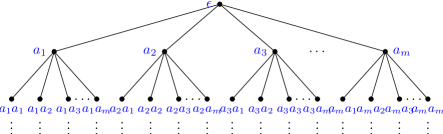
Figure 1. The vocabulary $\mathbf{A}^{*}$ as a rooted tree.

Each vertex of the tree corresponds to a word over the alphabet $\mathbf{A}$. That is, the set of vertices of the tree is $\mathbf{A}^{*}$. On the other hand, each infinite ray starting from the root, corresponds to an infinite sequence of symbols over $\mathbf{A}$, and it corresponds to the boundary of the tree. We denote this boundary by $\partial T$ and as mentioned, viewed as a set is equal to $\mathbf{A}^{\mathbb{N}}$.

The construction of the tree is unique up to the particular ordering of the symbols in $\mathbf{A}$ we chose. Thus, in principle, if $\gamma:\mathbf{A}\to\{0,\dots,m-1\}$ is a particular ordering (i.e. a bijection) of the alphabet where an element $a$ is denoted as $a_{i}$ if $\gamma(a)=i-1$, then the tree should be denoted by $T_{\gamma}$ as it depends on that particular ordering of the alphabet.

Let us denote by $T$ the regular rooted tree over the alphabet $\{0,1,\dots m-1\}$ with the natural order induced by $\mathbb{N}$ (see Fig. 2).

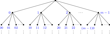
Figure 2. The regular rooted tree $T$ over the alphabet $\{0,1,\dots,m-1\}$.

Henceforth will denote by $\mathbf{M}$ the alphabet $\{0,\dots,m-1\}$ and as before, by $T$ the tree corresponding to the alphabet $\mathbf{M}$ under the usual ordering on $\mathbb{N}$.

When we say that the construction is unique up to reordering of symbols, we mean that both trees are isomorphic as graphs, where an isomorphism of graphs is a bijection between vertices preserving incidence. Indeed, for any bijection $\gamma:\mathbf{A}\to\mathbf{M}$, the tree $T_{\gamma}$ is ismorphic to $T$ as a graph.

Lemma 2.1.

Let $\gamma:\mathbf{A}\to\mathbf{M}$ be an ordering of the alphabet $\mathbf{A}$. Then $T_{\gamma}$ and $T$ are isomorphic.

Since being isomorphic is transtive, this lemma shows that for any two alphabets $\mathbf{A}_{1}$ and $\mathbf{A}_{2}$ of the same cardinality and any two orderings of those alphabets $\gamma_{1}$ and $\gamma_{2}$, their corresponding trees $T_{\gamma_{1}}$ and $T_{\gamma_{2}}$ will be isomorphic as graphs.

2.2.2. Gödel encodings

Having $\mathbf{A}^{\mathbb{N}}$, the space of one-sided infinite sequences over an alphabet $\mathbf{A}$ containing $|\mathbf{A}|=m$ symbols and $s=a_{1}a_{2}\ldots$ a sequence in this space, with $a_{k}$ being the $k$-th symbol in $s$ and an ordering $\gamma:\mathbf{A}\to\{0,\dots,m-1\}$, then a Gödelization is a mapping from $\mathbf{A}^{\mathbb{N}}$ to $[0,1]\subset\mathbb{R}$ defined as follows:

(10) $$\psi_{\gamma}(s):=\sum\limits_{k=1}^{\infty}\gamma(a_{k})m^{-k}.$$

By the Lemma 2.1 we know that for each Gödelization of $\mathbf{A}$ induced by $\gamma$, there is an isomorphism of graphs between $T_{\gamma}$ and $T$. Since the choice for the ordering of the alphabet (in other words, the choice of $\gamma$) is arbitrary and leads to different Gödel encodings, we are interested in finding invariants for different such encodings.

One can define a metric on the boundary of the tree in the following way: given any two infinite rays of the tree $p=a_{1}a_{2}a_{3}\dots$ and $q=b_{1}b_{2}b_{3}\dots$ we define

$$d(p,q)=\begin{cases}0&\text{ if }p=q\\ m^{-n},&\text{ if }a_{i}=b_{i}\text{ for }i=1,\dots,n\text{ and }a_{n+1}\neq b_{n+1}\\ 1&\text{ if }a_{1}\neq b_{1}.\end{cases}$$

This defines an ultrametric on the boundary, that is, a metric that satisfies a stronger version of the triangular inequality, namely:

$$d(p,q)\leq\max\{d(p,r),d(r,q)\}.$$

When we encode the infinite strings under the Gödel encoding, we are sending rays that are close to each other under this ultrametric to points that are close in the $[0,1]$ interval under the usual metric.

Lemma 2.2.

Let $p=a_{1}a_{2}a_{3}\dots$ and $q=b_{1}b_{2}b_{3}\dots$ be two infinite strings over $\mathbf{A}$. Then for any Gödel encoding $\psi$ we have that

$$d(p,q)\leq\frac{1}{m^{n}}\iff\exists k\in\{0,\dots,m^{n}-1\},\psi(p),\psi(q)\in\left[\frac{k}{m^{n}},\frac{k+1}{m^{n}}\right).$$

Recall that the lemma does not mean that points that are close (with respect to the usual metric) on the $[0,1]$ interval come from rays that were close on the tree. For example, if the alphabet has $3$ letters, the points $1/3-\epsilon$ and $1/3$ are as close as we want for any $\epsilon>0$ but are at distance $0$ from each other on the tree. In fact, it gives a partition of the interval for each $n\in\mathbb{N}$ in a way that, if two points representing an infinite string are in the same interval according to the partition of the corresponding $n$, then they come from two rays that share at least a common prefix of length $n$.

2.2.3. Cylinder sets

In symbolic dynamics, a cylinder set (McMillan 1953) is a subset of the space $\mathbf{A}^{\mathbb{N}}$ of infinite sequences from an alphabet $\mathbf{A}$ that agree in a particular building block of length $l\in\mathbb{N}$. Thus, let $w=\mathbf{A}^{*}$ be a finite word $a_{1}a_{2}\dots a_{l}$ of length $l$, we define the cylinder set

(11) $$[w]=[a_{1}a_{2}\dots a_{l}]=\{s\in\mathbf{A}^{\mathbb{N}}\,|\,s_{k}=a_{k},\quad k=1,\dots,l\}\>.$$

We can also see the cylinder sets on the tree depicted in Fig. 3. In fact, for each level on the tree (where level refers to vertices corresponding to words of certain fixed length) we get a partition of the interval $[0,1]$. The vertices hanging from each vertex on that level land on their corresponding interval of the partition. Thus, from a rooted tree view point, a cylinder set corresponds to a whole tree hanging from that vertex. Concretely, the cylinder set $[w]$ for the word $w\in\mathbf{A}^{*}$ is the subtree hanging from the vertex decorated by $w$.

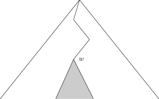
Figure 3. Cylinder set corresponding to $w$ seen on the tree.

Two different Gödel codes $\psi,\varphi$ can only differ with respect to their assignments $\gamma_{1},\gamma_{2}:\mathbf{A}\to\{0,\dots,m-1\}$. Thus, we call a permutation $\pi\in S_{m}$ (with $S_{m}$ as the symmetric group) a Gödel recoding, if

$$\pi\circ\gamma_{1}=\gamma_{2}\>.$$

2.2.4. Invariants

The ultimate goal of our study is to find invariants under Gödel recodings. Observe that under the notation of Lemma 2.1, $g_{\gamma_{1}}:T_{\gamma_{1}}\to T$ and $g_{\gamma_{2}}:T_{\gamma_{2}}\to T$ are two graph isomorphisms. In fact, they induce a graph automorphism of $T$, $g_{\pi}=g_{\gamma_{2}}\circ g_{\gamma_{1}}^{-1}:T\to T$. And this automorphism sends the vertices encoded by $\gamma_{1}$ to the ones encoded by $\gamma_{2}$.

As Lemma 2.2 shows, a Gödel recoding preserves the size of cylinder sets after permuting vertices. However, the way of ordering the alphabet and how this permutes the rays of the tree is even more restrictive than just preserving the size of the cylinder sets. In fact, under the action of a reordering each vertex can only be mapped to certain vertices and it is forbidden to be sent to others. This is captured by the following most central definition.

Definition 2.3.

Let $w=a_{i_{1}}a_{i_{2}}\dots a_{i_{l}}\in\mathbf{M}^{l}$ be a string of length $l$ after an ordering $\gamma$. We define a partition of the set of integers $\{1,2,\dots,l\}$,

(12) $$\mathcal{P}_{w}=\{\{j_{1},\dots,j_{k}\}\subset\mathbb{N}|a_{i_{j_{1}}}=\dots=a_{i_{j_{k}}}\}\>.$$

For any word $w\in\mathbf{M}^{*}$ we call $\mathcal{P}_{w}$ the pattern of equality of $w$.

Equipped with aforementioned formalisms we are now in a position to formulate the first main finding of our study as follows.

Theorem 2.4.

For any other vertex $u\in T$ there exists a Gödel recoding $\pi$ such that $g_{\pi}(w)=u$ if and only if

(13) $$u \in \mathbf{M}^{l}$$

(14) $$P_{w} = P_{u}\>.$$

Theorem 2.4 states that each vertex can be mapped to any vertex having the same pattern of equality and nowhere else.

Example 2.5.

If $\mathbf{A}=\{a,b,c\}$ and we consider $w=aaabcabc\in\mathbf{A}^{8}$. Then we have $P_{w}=\{\{1,2,3,6\},\{4,7\},\{5,8\}\}$, which gives us all the possible words where $w$ can be mapped to. That would be the list of all the possibilities:

$$\begin{matrix}bbbacbac&cccbacba&aaacbacb\\ bbbcabca&cccabcab&aaabcabc\end{matrix}$$

So we have only $6$ possible vertices out of $3^{8}=6561$. And of course, this proportion reduces as we go deeper on the tree.

In terms of Gödelization into the $[0,1]$ interval, we ilustrate the implications by an example. Let us assume that $m=3$ and $l=3$, for example. Then, in Fig. 4 the cylinder sets of certain color can only be mapped through a recoding to a cylinder set of the same color and nowhere else.

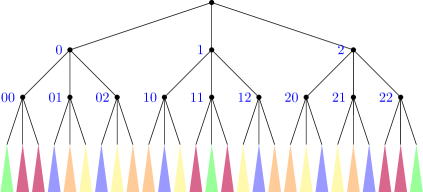
Figure 4. Invariant partition of the cylinder sets according to their patterns of equality.

Figure 5 shows the corresponding partition of the interval $[0,1]$ where the intervals in each color may be mapped to another of the same color by a different assignment map and nowhere else.

Figure 5. Invariant partition of the interval $[0,1]$ after Gödelization.

2.3. Neural automata

Following beim Graben et al (2004; 2008), and Carmantini et al (2017), a dotted sequence $s\in\mathbf{A}^{\mathbb{Z}}$ on an alphabet $\mathbf{A}$ is a two-sided infinite sequence of symbols “$s=\ldots\;a_{-2}\;a_{-1}\;.\;a_{0}\;a_{1}\;a_{2}\;\ldots$” where $a_{i}\in\mathbf{A}$, for all indices $i\in\mathbb{Z}$. Here, the dot “.” is simply used as a mnemonic sign, indicating that the index 0 is to its right.

Carmantini et al (2017) interpreted the dot as a meta-symbol which can be concatenated with two words $v_{1},v_{2}\in\mathbf{A}^{*}$ through $v=v_{1}.v_{2}$. Let $\hat{\mathbf{A}}^{*}$ denote the set of these dotted words. Moreover, let $\mathbb{Z}^{-}=\{i\;|\;i<0,\;i\in\mathbb{Z}\}$ and $\mathbb{Z}^{+}=\{i\;|\;i\geq 0,\;i\in\mathbb{Z}\}$ the sets of negative and non-negative indices. We can then reintroduce the notion of a dotted sequence as follows. Let $s\in\mathbf{A}^{\mathbb{Z}}$ be a bi-infinite sequence of symbols such that $s=w_{\alpha}vw_{\beta}$ with $v\in\hat{\mathbf{A}}^{*}$ as a dotted word $v=v_{1}.v_{2}$ and $w_{\alpha}v_{1}\in\mathbf{A}^{\mathbb{Z}^{-}}$ and $v_{2}w_{\beta}\in\mathbf{A}^{\mathbb{Z}^{+}}$. Through this definition, the indices of $s$ are inherited from the dotted word $v$ and are thus not explicitly prescribed.

A versatile shift (VS) was defined by Carmantini et al (2017) as a pair $M_{VS}=(\mathbf{A}^{\mathbb{Z}},\Omega)$, with $\mathbf{A}^{\mathbb{Z}}$ being the space of dotted sequences, and $\Omega:\mathbf{A}^{\mathbb{Z}}\rightarrow\mathbf{A}^{\mathbb{Z}}$ defined by

(15) $$\Omega(s)=\sigma^{F(s)}(s\oplus G(s))$$

with

(16) $$F:\mathbf{A}^{\mathbb{Z}}\rightarrow\mathbb{Z}$$

$$\oplus:\mathbf{A}^{\mathbb{Z}}\times\mathbf{A}^{\mathbb{Z}}\rightarrow\mathbf{A}^{\mathbb{Z}}$$

$$G:\mathbf{A}^{\mathbb{Z}}\rightarrow\mathbf{A}^{\mathbb{Z}},$$

where the operator “$\oplus$” substitutes the dotted word $v_{1}.v_{2}\in\hat{\mathbf{A}}^{*}$ in $s$ with a new dotted word $\hat{v_{1}}.\hat{v_{2}}\in\hat{\mathbf{A}}^{*}$ specified by $G$, while $F(s)=F|_{\hat{\mathbf{A}}^{*}}(v_{1}.v_{2})$ determines the number of shift steps as for Moore’s generalized shifts (Carmantini et al 2017).

A nonlinear dynamical automaton (NDA) is a triple $M_{NDA}=(Y,\mathcal{P},\Phi)$, where $\mathcal{P}$ is a rectangular partition of the unit square $Y={[0,1]}^{2}\subset\mathbb{R}^{2}$, that is

(17) $$\mathcal{P}=\{D^{(i,j)}\subset Y|~{}1\leq i\leq m,\;1\leq j\leq n,\;m,n\in\mathbb{N}\},$$

so that each cell is defined as $D^{(i,j)}=I_{i}\times J_{j}$, with $I_{i},J_{j}\subset[0,1]$ being real intervals for each bi-index $(i,j)$, with $D^{(i,j)}\cap D^{(k,l)}=\varnothing$ if $(i,j)\neq(k,l)$, and $\bigcup_{i,j}D^{(i,j)}=Y$. The couple $(Y,\Phi)$ is a time-discrete dynamical system with phase space $Y$ and the flow $\Phi:Y\rightarrow Y$ is a piecewise affine-linear map such that $\Phi_{|D^{(i,j)}}:=\Phi^{(i,j)}$, with $\Phi^{(i,j)}$ having the following form:

(18) $$\Phi^{(i,j)}(\mathbf{y})=\left(\begin{array}[]{c}a^{(i,j)}_{1}\\ a^{(i,j)}_{2}\end{array}\right)+\left(\begin{array}[]{cc}\lambda^{(i,j)}_{1}&0\\ 0&\lambda^{(i,j)}_{2}\end{array}\right)\left(\begin{array}[]{c}y_{1}\\ y_{2}\end{array}\right)\>,$$

with state vector $\mathbf{y}=(y_{1},y_{2})$. Carmantini et al (2017) have shown that using Gödelization any versatile shift can be mapped to a nonlinear dynamical automaton. Therefore, one can reproduce the activity of a versatile shift on the unit square $Y$. In order to do so, the partition (17) is given by the so called Domain of Dependance (DoD). The Domain of Dependance is a pair $(l,r)\in\mathbb{N}\times\mathbb{N}$ which defines the length of the strings on the left and right hand side of the dot in a dotted sequence that is relevant for the versatile shift to act on the phase space. The dynamics of the versatile shift is completely determined by how the string looks like in each iteration on the Domain of Dependance. Then, if the domain is $(l,r)$ and if the alphabet $\mathbf{A}$ has size $m$, the partition of the unit square is given by $m^{r}$ intervals on the $y_{1}$ axis and $m^{l}$ intervals on the $y_{2}$ axis, corresponding to cells where the NDA is defined according to the versatile shift. Finally, a neural automaton (NA) is an implementation of an NDA by means of a modular recurrent neural network (Carmantini et al 2017).

The neural automaton comprises a phase space $X=[0,1]^{n}$ where the two-dimensional subspace $Y=[0,1]^{2}$ of the underlying NDA is spanned by only two neurons that belong to the machine configuration layer (MCL). The remainder $X\setminus Y$ is spanned by the neurons of the branch selection layer (BSL) and the linear transformation layer (LTL), both mediating the piecewise affine mapping (18). Having an NDA defined from a versatile shift, each rectangle on the partition is given by the DoD, and the action of the NDA on each rectangle depends on the particular Gödel encoding of the alphabet $\mathbf{A}$ that has been chosen. We are interested in invariant macroscopic observables of such automata under different Gödel encodings of the alphabet.

Since we are now interested on dotted sequences over an alphabet $\mathbf{A}$, instead of having an invariant partition of the interval $[0,1]$ as in Fig. 5, we will have an invariant partition of the unit square $Y=[0,1]^{2}$. That is, we will have a partition in rectangles where the machine might be at certain step of the dynamics or not. Each color in that partition gives all the possible places where a particular dotted sequence of certain right and left lengths could be under a different Gödel encoding.

For example, assuming that our alphabet has $m=3$ letters in both sides of the dotted sequence and that we are looking at words of length $l=2$ on the left hand side of the dot, and length $r=3$ on the right hand side of the dot, the partition would be like in Figure 6.

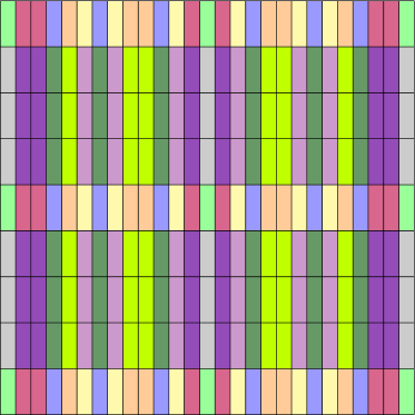
Figure 6. Each small square corresponds to a square on the partition given by the dotted sequences of length $(2,3)$. The squares colored by the same color are those having the same pattern of equality, and thus, are those which can be mapped to each other under different Gödel encodings of the alphabet.

Let us assume that we are considering the invariant partition for dotted sequences of length $(l,r)$, meaning that the left hand side has length $l$ and the right hand side $r$. Then we know that the partition of the square $Y$ is given by $E^{(i,j)}=\left[\frac{i}{m^{l}},\frac{i+1}{m^{l}}\right)\times\left[\frac{j}{m^{r}},\frac{j+1}{m^{r}}\right)$. Each left corner of the rectangle corresponds to the position of the Gödelization of a dotted sequence of size $(l,r)$. Each point $(y_{1},y_{2})=(\frac{i}{m^{l}},\frac{j}{m^{l}})$ has a unique expansion on base $m$ for its coordinates. That is, there are some $c_{1},\dots,c_{l}$ with $0\leq c_{i}\leq m_{1}$ such that

(19) $$y_{1}=\frac{i}{m^{l}}=\frac{c_{1}}{m}+\frac{c_{2}}{m^{2}}+\dots+\frac{c_{l}}{m^{l}}.$$

These $\{c_{1},\dots,c_{l}\}$ also define a partition of $\{1,\dots,l\}$ in the same way as given in definition 2.3. Therefore $\{d_{1},\dots,d_{k}\}\in\mathcal{P}_{x}\iff c_{j_{1}}=\dots=c_{j_{k}}$. This procedure similarly applies to the $y_{2}$ coordinate. Hence, the corners defining an invariant piece of the partition will be those sharing the same partition of $\{1,\dots,l\}\times\{1,\dots,r\}$. In other words, we can obtain the corners related to a given $\mathbf{y}$ by expanding $y_{1}$ and $y_{2}$ on base $m$ and permuting the appearance of $0,\dots,m-1$ on the expansion.

For example, if $m=3$ and $(l,r)=(2,3)$, we have $3^{2}\cdot 3^{3}=3^{5}$ rectangles. Now let us take, for instance the rectangle $\left[\frac{6}{3^{2}},\frac{7}{3^{2}}\right)\times\left[\frac{10}{3^{3}},\frac{11}{3^{3}}\right)$ and let us find its invariant partition. First we decompose

$$y_{1}=\frac{6}{3^{2}}=\frac{2}{3}+\frac{0}{9}\,\,\,\text{and}\,\,y_{2}=\frac{10}{3^{3}}=\frac{1}{3}+\frac{0}{9}+\frac{1}{27}.$$

Hence a rectangle in the same invariant partition must be of the form $E^{(i,j)}=\left[\frac{i}{m^{l}},\frac{i+1}{m^{l}}\right)\times\left[\frac{j}{m^{r}},\frac{j+1}{m^{r}}\right)$ with $\frac{i}{3^{2}}=\frac{a}{3}+\frac{b}{9}$ and $\frac{j}{3^{3}}=\frac{c}{3}+\frac{b}{9}+\frac{c}{27}$ with $a,b,c\in\{0,1,2\}$ and different. This gives the following rectangles

$$\left[\frac{1}{9},\frac{2}{9}\right)\times\left[\frac{23}{27},\frac{24}{27}\right) \left[\frac{3}{9},\frac{4}{9}\right)\times\left[\frac{20}{27},\frac{21}{27}\right)$$

$$\left[\frac{2}{9},\frac{3}{9}\right)\times\left[\frac{16}{27},\frac{17}{27}\right) \left[\frac{6}{9},\frac{7}{9}\right)\times\left[\frac{10}{27},\frac{11}{27}\right)$$

$$\left[\frac{7}{9},\frac{8}{9}\right)\times\left[\frac{3}{27},\frac{4}{27}\right) \left[\frac{5}{9},\frac{6}{9}\right)\times\left[\frac{6}{27},\frac{7}{27}\right)$$

In this way we can construct the partition of the unit square given by the patterns of equality.

2.3.1. Invariant observables

Our aim now is to define an observable $f\in B(X)$, in the sense of Section 2 for neural automata. That is $f:X\to\mathbb{R}$ should obey Eq. (3) where the map $\alpha^{*}_{\pi}$ corresponds to a symmetry induced by a Gödel recoding of the alphabets. Here $\pi$ denotes the permutation of the alphabet needed to pass from one Gödel encoding to the other, as explained later.

Notice that in the previous discussion we were assuming that we knew the length of the strings that were encoded. However, this is not the case in practice, and may cause problems, as the length of the strings vary at each iteration. For instance, if for the alphabet $\{a,b\}$ the symbol $a$ is mapped to $0$ under certain Gödel enconding $\gamma$ and the symbol $b$ to $1$, then the number $x=1/2\in[0,1]$ would correspond to the word $w_{r}=ba\overset{r-1}{\dots}a$ once we assume that the string is of length $r$ for $r\in\mathbb{N}\cup\{0\}$. However, if we do not know the length of the encoded string, each $w_{r}$ will have a different Gödel number under the Gödel encoding that sends $b$ to $0$ and $a$ to $1$, namely $\sum_{k=2}^{r-1}1/2^{k}$. Thus, encoding symbols with the number $0$ makes some strings indistinguishible under Gödel recoding, because having no symbols is interpreted as having the symbol encoded by $0$ as many times as we want. This issue can be easily avoided by adding one symbol $\sqcup$ to the alphabet, which will be interpreted as a blank symbol, and will always be forced to be encoded as $0$ by any Gödel encoding.

Suppose that we have an NDA defined from a versatile shift under the condition that the blank symbol $\sqcup$ has been added to the alphabet $\mathbf{A}$ representing the blank symbol and that is mapped to $0$ under any Gödel encoding. We will assume that $\mathbf{A}$ has $m$ symbols after adding the blank symbol (that is, we had $m-1$ symbols before). Then for any pair $(r,l)\in\mathbb{N}\times\mathbb{N}$, we can divide the unit square $Y$ into the rectangle partition given by

(20) $$\mathcal{R}=\{E^{(i,j)}\subset Y|~{}1\leq i\leq m^{r},\;1\leq j\leq m^{l}\}.$$

Next, we extend this partition of the phase space of the NDA, that equals the subspace of the machine configuration layer of the larger NA, to the entire phase space of the neural automaton. This is straightforwardly achieved by defining another partition

(21) $$\mathcal{Q}=\{E^{(i,j)}\times[0,1]^{n-2}\subset X|~{}1\leq i\leq m^{r},\;1\leq j\leq m^{l}\}.$$

Now, for each left corner $(x_{1}^{(i,j)},x_{2}^{(i,j)})\in E^{(i,j)}$ we find their pattern of equality $\mathcal{P}_{ij}$, assuming that the permutation is taking place just on the symbols $\{2,\dots,m\}$ (as the first symbol has to be mapped to $0$ under any encoding).

Let us suppose that $\{\mathcal{P}_{ij_{1}},\dots,\mathcal{P}_{ij_{s}}\}$ are all the different appearing patterns of equality and we define the indicator functions $\chi_{k}:X\to\{0,1\}$ as

(22) $$\chi_{k}(\mathbf{x})=\begin{cases}1&\text{if }\mathbf{x}\in E^{(i,j)}\times[0,1]^{n-2}\text{ and }\mathcal{P}_{ij}=\mathcal{P}_{ij_{k}}\\ 0&\text{otherwise}\end{cases}$$

for $\mathbf{x}\in X$. Then, we can choose $c_{1},\dots,c_{s}\in\mathbb{R}$ to be $s$ different real numbers and define a macroscopic observable $f:X\to\mathbb{R}$ as a step function

(23) $$f(\mathbf{x})=\sum_{k=1}^{s}c_{k}\chi_{k}(\mathbf{x})\>.$$

Clearly, we have $f\in B(X)$.

Our aim is to show that this observable is invariant under the symmetry group $S_{m-1}\times S_{m-1}$ of the dynamical system $(X,\Phi)$ given by the neural automaton in Eq. (18), where $S_{m-1}$ denotes the symmetric group on $m-1$ elements. First of all, we must show that $S_{m-1}\times S_{m-1}$ is a symmetry of the neural automaton.

Before doing this, we will define an auxiliary map. Let $\pi=(\pi_{1},\pi_{2})\in S_{m}\times S_{m}$ be any element of the product that fixes $1$ (on the set $\{1,2,\dots,m\}$ where $S_{m}$ acts). Notice that the elements of $S_{m}$ fixing the first element form a subgroup of $S_{m}$ that is isomorphic to $S_{m-1}$. Let now $\mathbf{x}$ be any point in $X$. Let us consider $\mathbf{y}=(y_{1},y_{2})$ the first two coordinates of $\mathbf{x}$ given by the activations of the machine configuration layer of the NA. Then, we can check in which of the intervals of the partition $\mathcal{R}$ is, say $(y_{1},y_{2})\in E^{(i,j)}=\left[\frac{i}{m^{l}},\frac{i+1}{m^{l}}\right)\times\left[\frac{j}{m^{r}},\frac{j+1}{m^{r}}\right)$. We can therefore compute the expansion on base $m$ of each corner and take the coefficients we get as words over the alphabet $\mathbf{M}=\{0,1,\dots,m-1\}$, say $c_{1}\dots c_{l}\in\mathbf{M}^{l}$ and $d_{1},\dots,d_{r}\in\mathbf{M}^{r}$. Then, we compute $g_{\pi_{1}}(c_{1}\dots c_{l})$ and $g_{\pi_{2}}(d_{1}\dots d_{r})$ and we encode these words by the canonical Gödel encoding (that is, the one given by the identity map on $\mathbf{M}$). Thus, we obtain a new corner of some rectangle in our partition of the phase space, say $E^{(i^{\prime},j^{\prime})}=\left[\frac{i^{\prime}}{m^{l}},\frac{i^{\prime}+1}{m^{l}}\right)\times\left[\frac{j^{\prime}}{m^{r}},\frac{j^{\prime}+1}{m^{r}}\right)$. We now define a map $\rho_{\pi}:Y\to Y$ by $\rho_{\pi}(y_{1},y_{2})=\left(y_{1}+\frac{i^{\prime}-i}{m^{l}},y_{2}+\frac{j^{\prime}-j}{m^{r}}\right)$. This map can obviously be extended to a map from $X$ to $X$ being the identity on the rest of the coordinates. Abusing notation we also refer to $\rho_{\pi}$ as to this map. Informally speaking, the map $\rho_{\pi}$ rigidly permutes the squares on the partition $\mathcal{R}$ according to the action of $g_{\pi_{1}}$ and $g_{\pi_{2}}$ on the words representing the corners.

Now, we can define $\alpha_{\pi}:B(X)\to B(X)$ as follows. For any $f\in B(X)$, we define

(24) $$\alpha_{\pi}(f)(\mathbf{x})=f(\rho_{\pi}(\mathbf{x}))\>.$$

It is not difficult to check that if $\pi,\gamma\in S_{m-1}\times S_{m-1}$ are two group elements, then $\alpha_{\gamma\pi}(f)=(\alpha_{\gamma}\circ\alpha_{\pi})(f)$ so that $S_{m-1}\times S_{m-1}$ is a symmetry of the system.

Thus, we obtain finally our main result.

Theorem 2.6.

Let $f\in B(X)$ be a macroscopic observable on the space space of a neural automaton as defined in (23). Then $f$ is invariant under the symmetric group $S_{m-1}\times S_{m-1}$ of Gödel recodings of the automaton’s symbolic alphabet.

It is worth mentioning that this procedure gives infinitely many different invariant observables. In fact, any choice of $(r,l)\in\mathbb{N}\times\mathbb{N}$ gives a thinner invariant partition, and respectively, a sharper observable.

3. Neurolinguistic application

As an instructive example we consider a toy model of syntactic language processing as often employed in computational psycholinguistics and computational neurolinguistics (Arbib and Caplan 1979, Crocker 1996, beim Graben and Drenhaus 2012, Hale et al 2022, Lewis 2003).

In order to process the sentence given by beim Graben and Potthast (2014) in example 3.1, linguists often derive a context-free grammar (CFG) from a phrase structure tree (Hopcroft and Ullman 1979).

Example 3.1.

the dog chased the cat

In our case, the CFG consists of rewriting rules

(25) S $$\to\text{\tt NP \ VP}$$

(26) VP $$\to\text{\tt V \ NP}$$

(27) NP $$\to\text{\tt the \ dog}$$

(28) V $$\to\text{\tt chased}$$

(29) NP $$\to\text{\tt the \ cat}$$

where the left-hand side always presents a nonterminal symbol to be expanded into a string of nonterminal and terminal symbols at the right-hand side. Omitting the lexical rules (27 – 29), we regard the symbols $\text{\tt NP},\text{\tt V}$, denoting ‘noun phrase’ and ‘verb’, respectively, as terminals and the symbols S (‘sentence’) and VP (‘verbal phrase’) as nonterminals.

Then, a versatile shift processing this grammar through a simple top down recognizer (Hopcroft and Ullman 1979) is defined by

(30) $$\begin{array}[]{l @{\:\mapsto\:}l }\text{\tt S}.a\hfil\>\mapsto\>&\text{\tt VP}\>\text{\tt NP}.a\\ \text{\tt VP}.a\hfil\>\mapsto\>&\text{\tt NP}\>\text{\tt V}.a\\ a.a\hfil\>\mapsto\>&\epsilon.\epsilon\end{array}$$

where the left-hand side of the tape is now called ‘stack’ and the right-hand side ‘input’. In (30) $a$ stands for an arbitrary input symbol. Note the reversed order for the stack left of the dot. The first two operations in (30) are predictions according to a rule of the CFG while the last one is an attachment of subsequent input with already predicted material.

This machine then parses the well formed sentence NP  V  NP as shown in Table 1 from beim Graben and Potthast (2014). We reproduce this table here as Tab. 1.

Table 1. Sequence of state transitions of the versatile shift processing the well-formed string from example 3.1, i.e. NP V NP. The operations are indicated as follows: “predict (X)” means prediction according to rule (X) of the context-free grammar; attach means cancelation of successfully predicted terminals both from stack and input; and “accept” means acceptance of the string as being well-formed.

time	state		operation
0	S .	NP V NP	predict (25)
1	VP NP .	NP V NP	attach
2	VP .	V NP	predict (26)
3	NP V .	V NP	attach
4	NP .	NP	attach
5	$\epsilon$ .	$\epsilon$	accept

Once we obtained the versatile shift, an NA simulating it can be generated. When we do so, we chose a particular Gödel encoding of the symbols. Suppose we chose the following two Gödelizations $\gamma=(\gamma_{1},\gamma_{2})$ and $\delta=(\delta_{1},\delta_{2})$ that are given by

$$\gamma_{1}:\{\sqcup,\text{\tt NP},\text{\tt V}\} \to\{0,1,2\}$$

$$\sqcup \mapsto 0$$

NP $$\mapsto 1$$

V $$\mapsto 2$$

$$\gamma_{2}:\{\sqcup,\text{\tt NP},\text{\tt V},\text{\tt VP},\text{\tt S}\} \to\{0,1,2,3,4\}$$

$$\sqcup \mapsto 0$$

NP $$\mapsto 1$$

V $$\mapsto 2$$

VP $$\mapsto 3$$

S $$\mapsto 4$$

on the one hand, and by

$$\delta_{1}:\{\sqcup,\text{\tt NP},\text{\tt V}\} \to\{0,1,2\}$$

$$\sqcup \mapsto 0$$

NP $$\mapsto 2$$

V $$\mapsto 1$$

$$\delta_{2}:\{\sqcup,\text{\tt NP},\text{\tt V},\text{\tt VP},\text{\tt S}\} \to\{0,1,2,3,4\}$$

$$\sqcup \mapsto 0$$

NP $$\mapsto 4$$

V $$\mapsto 3$$

VP $$\mapsto 1$$

S $$\mapsto 2$$

on the other hand. Defining the step function $f:X\to\mathbb{R}$ as in (23) after choosing $(l,r)=(2,3)$ and the $c_{i}$-s randomly. The neural automaton consists of $n=72$ neurons, i.e. the phase space is given by the hypercube $X=[0,1]^{72}$. Running the neural network with both encodings and computing the step function $f$ on each iteration $i=1,\dots,6$, we see in Fig. 7 that $f$ is indeed invariant under Gödel recoding.

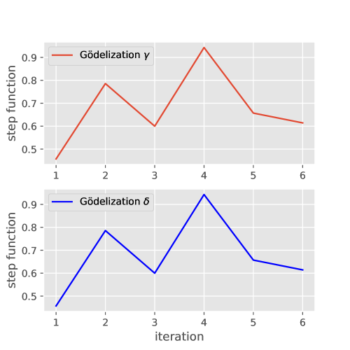
Figure 7. The macroscopic observable $f$, given by the step function (23) is invariant under Gödel recoding. The figure shows the result of ‘measuring’ $f$ to a neural automaton encoded by $\gamma$ on top and to the same machine encoded by $\delta$ below.

The step function clearly distinguishes among different states (where here by “different” we mean with different patterns of equality), but returns the same value for the states corresponding to the same pattern of equality, that is, states that differ on the Gödel encodings, as desired.

In contrast, if we use Amari’s observable Eq. (9) for the same simulation, we obtain a very different picture, showing that this observable is not invariant under Gödel recoding, as shown in Fig. 8. Obviously, this observable strongly depends on the particular Gödel encoding we have chosen.

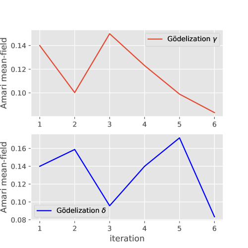
Figure 8. Amari’s mean-field observable Eq. (9) of the neural automaton under two different Gödel encodings $\gamma$ and $\delta$.

4. Discussion

In this study we have presented a way of finding particular macroscopic observables for nonlinear dynamical systems that are generated by Gödel encodings of symbolic dynamical systems, such as nonlinear dynamical automata (NDA: beim Graben et al (2000; 2004; 2008), beim Graben and Potthast (2014)) and their respective neural network implementation, namely, neural automata (NA: Carmantini et al (2017)). Specifically, we have investigated under which circumstances such observables could be invariant under any particular choice for the Gödel encoding.

When mapping symbolic dynamics to a real phase space, the numbering of the symbols is usually arbitrary. Therefore, it makes sense to ask which information of the dynamics is preserved or can be recovered from what we see in phase space under the different possible options. In this direction, we have provided a complete characterisation of the strings that are and are not distinguishable after certain Gödel encoding in terms of patterns of equality. We have proven a partition theorem for such invariants.

In the concrete case of NA constructed as in Carmantini et al (2017), which can emulate any Turing Machine, we have a dynamical system for a neural automaton. This system completely depends on the choice of the Gödel numbering for the symbols on the alphabet of the NA. Based on the invariant partition mentioned before, we were able to define a macroscopic observable that is invariant under any Gödel recoding. In fact, by the way we define this observable, the definition is based on an invariant partition according to the length of the strings on the left and right hand side of a dotted sequence compising the machine tape of the NA. This means that each choice of the length of those strings provides a sharper invariant, making strings with different patterns of equality completely distinguishable. It is also important to mention that macroscopic observables in general are not invariant under Gödel recoding. As a particular example, we computed the mean neural network activation originally suggested by Amari (1974) and later employed by Carmantini et al (2017) as a modeled “synthetic ERP” (Barrès et al 2013) in neurocomputing.

In fact, any observable that is invariant under Gödel recoding must be equally defined for points on the phase space corresponding to Gödelizations of strings sharing the same patterns of equality. This could probably provide an important constraint in the finding of other invariant macroscopic observables.

Theoretically, one could run neural automaton under all (or many) possible Gödel encodings and check which observables are preserved by the dynamics and which are not. This could provide important information about the performance of the neural network architecture that is intrinsic of the dynamical system, and not dependant on the choice of the numbering for the codification of the symbols. In practice, the computation of all the permutations of the alphabet grows with the factorial of the alphabet’s cardinality, and the computation of invariant partitions even with powers of that number for longer strings. This, of course, would present some practical constraints for large alphabets and sharp invariant observables.

Our results could be of substantial importance for any kind of related approaches in the field of computational cognitive neurodynamics. All models that rely upon the representation of symbolic mental content by means of high-dimensional activation vectors as training patterns for (deep) neural networks (Arbib 1995, LeCun et al 2015, Hertz et al 1991, Schmidhuber 2015), such as vector symbolic architectures (Gayler 2006, Schlegel et al 2021, Smolensky 1990; 2006, Mizraji 1989; 2020) in particular, are facing the problems of arbitrary symbolic encodings. As long as one is only interested in building inference machines for artificial intelligence, this does not really matter. However, when activation states of neural network simulations have to be correlated with real-word data from experiments in the domains of human or animal cognitive neuroscience and psychology, the given encoding may play a role. Thus, the investigation of invariant observables in regression analyses and statistical modeling becomes mandatory for avoiding possible confounds that could result from a particularly chosen encoding.

These results also have implications in Mathematical and Computational Neuroscience, where the aim is to explain by means of mathematical theories and computational modelling neurophysiological processes as observed in in-vitro and in-vivo experiments via instrumentation devices. Our results forces us to consider the possibility as to what extent (if any) that observations, which motivate the development of models in the literature (e.g Spiking models), are epiphenomenon? To conclude, we express the hope that our study paves the way towards a more a comprehensive research in computational cognitive neurodynamics, mathematical and computational neuroscience where the study of macroscopic observations and its invariant formulation can lead to interesting new insights.

4.1. Reproducibility

All numerical simulations that have been presented in Section 3 may be reproduced using the code available at the Github repository https://github.com/TuringMachinegun/Turing_Neural_Networks. The repository contains the code to build the architecture of a neural automaton as introduced in (Carmantini et al (2017)) together with particular examples. The code that computes the invariant partitions given by equality patterns can also be found in the repository. The code allows the user to implement various observables (e.g step function, Amari’s observable) in order to test further cases, exploit and further develop our framework.

5. Acknowledgements

SR acknowledges support from Ikerbasque (The Basque Foundation for Science), the Basque Government through the BERC 2022-2025 program and by the Ministry of Science and Innovation: BCAM Severo Ochoa accreditation CEX2021-001142-S / MICIN / AEI / 10.13039/501100011033 and through project RTI2018-093860-B-C21 funded by (AEI/FEDER, UE) and acronym MathNEURO. JUA aknowledges support from the Spanish Government, grants PID2020-117281GB-I00 and PID2019-107444GA-I00, partly with European Regional Development Fund (ERDF), and the Basque Government, grant IT1483-22.

Appendix A Proofs of lemmata and theorems

of Lemma 2.1.

The ordering $\gamma$ itself induces the isomorphism between both graphs. Namely let $g_{\gamma}:T_{\gamma}\to T$ be such that if $s=a_{i_{1}}a_{i_{2}}a_{i_{3}}\dots\in T_{\gamma}$ then

$$g_{\gamma}(s)=\gamma(a_{i_{1}})\gamma(a_{i_{2}})\gamma(a_{i_{3}})\dots$$

which clearly belongs to $T$.

We must show that it defines a bijection between vertices and that preserves incidence.
It is easy to prove that it is a bijection. Namely if $w=a_{i_{1}}a_{i_{2}}\dots a_{i_{n}}$ and $u=b_{i_{1}}\dots b_{i_{k}}$ are any two vertices of the tree $T_{\gamma}$ then $g_{\gamma}(w)=g_{\gamma}(u)$ implies that both strings must have the same length, hence $n=k$. And since $\gamma(a_{i_{j}})=\gamma(b_{i_{j}})$ and $\gamma$ is a bijection, we must have $a_{i_{j}}=b_{i_{j}}$ so that $w=u$. Moreover, for any $v=l_{1}\dots l_{n}\in T$ there is $z=a_{\gamma^{-1}(l_{1})}\dots a_{\gamma^{-1}(l_{n})}$ which is clearly mapped to $v$ through $g_{\gamma}$.

The only thing that is left to show is that $g_{\gamma}$ preserves incidence. That is, that given $w\in\mathbf{A}^{*}$ and $a\in\mathbf{A}$, then $g_{\gamma}(wa)=g_{\gamma}(w)l$ for some $l\in\{0,\dots,m-1\}$. But this is also clear from the definition of $g_{\gamma}$. ∎

of Lemma 2.2.

Let us suppose that $d(p,q)\leq\frac{1}{m^{n}}$. This means that at least the first $n$ symbols in both strings are equal. Then, if $\psi$ is a Gödel encoding defined by the asignment $\gamma:\mathbf{A}\to\mathbf{M}$ we have that

$$\psi(p)=\sum\limits_{i=1}^{\infty}\gamma(a_{i})\frac{1}{m^{i}}=\sum\limits_{i=1}^{n}\gamma(a_{i})\frac{1}{m^{i}}+\sum\limits_{i=n+1}^{\infty}\gamma(a_{i})\frac{1}{m^{i}}.$$

Let us put $r=\sum\limits_{i=1}^{n}\gamma(a_{i})\frac{1}{m^{i}}$. Now, since $\gamma(a_{i})\leq m-1$

$$r =\frac{a_{1}m^{n-1}+a_{2}d^{n-2}+\dots a_{n-1}m+a_{n}}{m^{n}}\leq$$

$$\leq\frac{m^{n}-m^{n-1}+m^{n-1}-\dots-d+d-1}{m^{n}}=\frac{m^{n-1}}{m^{n}}.$$

So $r=\frac{k}{m^{n}}$ for some $k=0,\dots,m^{n}-1$. Since $\sum\limits_{i=n+1}^{\infty}\gamma(a_{i})\frac{1}{m^{i}}<\frac{1}{m^{n+1}}$, we get that $\psi(p)\in\left[\frac{k}{m^{n}},\frac{k+1}{m^{n}}\right)$. Since $q$ is equal to $p$ on at least the first $n$ strings we will also have $\psi(q)=r+\sum\limits_{i=n+1}^{\infty}\gamma(b_{i})\frac{1}{m^{i}}$ and by the same reason it will be on the same interval.

For the other implication, if we have two real numbers $\psi(p)$ and $\psi(q)$ after encoding some infinite strings $p$ and $q$, we want to show that if they are on some interval of the type $\left[\frac{k}{m^{n}},\frac{k+1}{m^{n}}\right)$, then they have the same prefix of at least length $n$. We can always write those numbers as $\psi(p)=\frac{k}{m^{n}}+r_{1}$ and $\psi(q)=\frac{k}{m^{n}}+r_{2}$ with $r_{1},r_{2}<\frac{1}{m^{n+1}}$. If we write the number $k$ in its $m$-adic expansion, it will be uniquely determined by $l_{1},\dots,l_{n}\in\{0,\dots,m-1\}$, and each number $r_{i}$ can be writen as a series by $r_{i}=\sum\limits_{j=n+1}l_{j_{i}}\frac{1}{m^{j}}$, for $i=1,2$. Taking the inverse images of each $l_{i}$, that is $\gamma^{-1}(l_{i})=a_{i}$ we will obtain that $p=a_{1}\dots a_{n}a_{n+1}\dots$ and $q=a_{1}\dots a_{n}b_{n+1}\dots$. That is, they are at least at distance $\frac{1}{m^{n}}.$ ∎

of Theorem 2.4.

Let us first assume that given $u$ there exists some $\pi$ such that its induced automorphisms maps $w$ to $u$. The condition Eq. (13) is clear, by Lemma 2.2. Then, we can write $u=c_{1}\dots c_{n}$. Now, we know that $g_{\pi}(w)=a_{\pi(1)}a_{\pi(2)}\dots a_{\pi(n)}=c_{1}\dots c_{n}=u$. Then

$$\{j_{1},\dots,j_{k}\}\in P_{w} \iff a_{i_{j_{1}}}=\dots=a_{i_{j_{k}}}$$

$$\iff a_{\pi(i_{j_{1}})}=\dots=a_{\pi(i_{j_{k}})}$$

$$\iff c_{i_{j_{1}}}=\dots=c_{i_{j_{k}}}$$

$$\iff\{j_{1},\dots,j_{k}\}\in P_{u}.$$

To show the other direction, it suffices to define $\pi$ so that $g_{\pi}(w)=u$. That is, if $u=c_{1}\dots c_{n}$, let us define $\pi(a_{i})=c_{i}$ and let us send the $a_{j}\in\mathbf{M}$ not appearing in $w$ to the $c_{j}$-s not appearing in $u$ in a bijective way. This can be done, it is well defined by condition Eq. (14), and it defines a bijection on $\mathbf{M}$ by construction. ∎

of Theorem 2.6.

We have to show that equation (3) is satisfied. Namely, we have to show that $f(\alpha^{*}_{\pi}(\mathbf{x}))=f(\mathbf{x})$ for each $\pi\in S_{m-1}\times S_{m-1}$ and $\mathbf{x}\in X$. Note that by definition, $\alpha^{*}_{\pi}=\rho_{\pi}$ in our case. Therefore, we must show that $f(\rho_{\pi}(\mathbf{x}))=f(\mathbf{x})$ Let $\pi=(\pi_{1},\pi_{2})\in S_{m-1}\times S_{m-1}$ and $(y_{1},y_{2})\in Y$. Then, there is some $E^{(i,j)}$ for which $(x,y)\in E^{(i,j)}$. Let us denote by $\pi^{\prime}=(\pi^{\prime}_{1},\pi^{\prime}_{2})\in S_{m}\times S_{m}$ the permutation fixing $1$ and sending $\pi^{\prime}(i)=\pi(i)+1$ for $i=2,\dots,m-1$ (namely, the permutation fixing the first letter and permuting the rest as $\pi_{i}$ permutes the $m-1$ letters for $i=1,2$ respectively).

Note that since we have enlarged our alphabet with the $\sqcup$ symbol, and since both our original encoding and the one permuted by $\pi$ send this symbol to $0$, if $(y_{1},y_{2})$ is decoded as $(c_{1},\dots,c_{l})$ and $(d_{1},\dots,d_{r})$, the possible $0$s appearing at the end of each encoding (indicating that the string has smaller length than $l$ and/or $r$) will remain being $0$-s, and therefore the point will not be mapped to a point encoding longer strings.

After applying $\rho_{\pi^{\prime}}$, we will obtain $\rho_{\pi}((y_{1},y_{2}))\in E^{(i^{\prime},j^{\prime})}$ for some $i^{\prime},j^{\prime}$. However, since $\rho_{\pi^{\prime}}$ is defined through $g_{\pi^{\prime}_{1}}$ and $g_{\pi^{\prime}_{2}}$ both $E^{(i,j)}$ and $E^{(i^{\prime},j^{\prime})}$ belong to the same $P_{ij}$. That is, they have the same pattern of equality. Hence, by the definition of $f$ we obtain that $f(\mathbf{x})=f(\rho_{\pi}(\mathbf{x}))$, and we are done. ∎

References

- Amari (1974) Amari SI (1974) A method of statistical neurodynamics. Kybernetik 14:201 – 215
- Anderson et al (2004) Anderson JR, Bothell D, Byrne MD, Douglass S, Lebiere C, Qin Y (2004) An integrated theory of the mind. Psychological Review 111(4):1036 – 1060
- Arbib (1995) Arbib MA (ed) (1995) The Handbook of Brain Theory and Neural Networks. MIT Press, Cambridge (MA)
- Arbib and Caplan (1979) Arbib MA, Caplan D (1979) Neurolinguistics must be computational. Behavioral and Brain Sciences 2(03):449 – 460
- Atmanspacher and beim Graben (2007) Atmanspacher H, beim Graben P (2007) Contextual emergence of mental states from neurodynamics. Chaos and Complexity Letters 2(2/3):151 – 168
- Barrès et al (2013) Barrès V, III AS, Arbib M (2013) Synthetic event-related potentials: A computational bridge between neurolinguistic models and experiments. Neural Networks 37:66 – 92
- Boston et al (2008) Boston MF, Hale JT, Patil U, Kliegl R, Vasishth S (2008) Parsing costs as predictors of reading difficulty: An evaluation using the Potsdam Sentence Corpus. Journal of Eye Movement Research 2(1):1 – 12
- Brouwer and Crocker (2017) Brouwer H, Crocker MW (2017) On the proper treatment of the P400 and P600 in language comprehension. Frontiers in Psychology 8:1327
- Brouwer and Hoeks (2013) Brouwer H, Hoeks JCJ (2013) A time and place for language comprehension: mapping the N400 and the P600 to a minimal cortical network. Frontiers in Human Neuroscience 7(758)
- Brouwer et al (2012) Brouwer H, Fitz H, Hoeks J (2012) Getting real about Semantic Illusions: Rethinking the functional role of the P600 in language comprehension. Brain Research 1446:127 – 143
- Brouwer et al (2017) Brouwer H, Crocker MW, Venhuizen NJ, Hoeks JCJ (2017) A neurocomputational model of the N400 and the P600 in language processing. Cognitive Science 41(S6):1318 – 1352
- Brouwer et al (2021) Brouwer H, Delogu F, Venhuizen NJ, Crocker MW (2021) Neurobehavioral correlates of surprisal in language comprehension: A neurocomputational model. Frontiers in Psychology 12:110
- Carmantini et al (2017) Carmantini GS, beim Graben P, Desroches M, Rodrigues S (2017) A modular architecture for transparent computation in recurrent neural networks. Neural Networks 85:85 – 105
- Cleeremans et al (1989) Cleeremans A, Servan-Schreiber D, McClelland JL (1989) Finite state automata and simple recurrent networks. Neural Computation 1(3):372 – 381
- Crocker (1996) Crocker MW (1996) Computational Psycholinguistics, Studies in Computational Psycholinguistics, vol 20. Kluwer, Dordrecht
- Davidson and Martin (2013) Davidson DJ, Martin AE (2013) Modeling accuracy as a function of response time with the generalized linear mixed effects model. Acta Psychologica 144(1):83 – 96
- Elman (1990) Elman JL (1990) Finding structure in time. Cognitive Science 14:179 – 211
- Elman (1991) Elman JL (1991) Distributed representations, simple recurrent networks, and grammatical structure. Machine Learning 7:195 – 225
- Emch (1964) Emch G (1964) Coarse-graining in Liouville space and master equation. Helvetica Physica Acta 37:532 – 544
- Frank et al (2015) Frank SL, Otten LJ, Galli G, Vigliocco G (2015) The ERP response to the amount of information conveyed by words in sentences. Brain and Language 140:1 – 11
- Frisch et al (2004) Frisch S, beim Graben P, Schlesewsky M (2004) Parallelizing grammatical functions: P600 and P345 reflect different cost of reanalysis. International Journal of Bifurcation and Chaos 14(2):531 – 549
- Friston et al (2000) Friston KJ, Mechelli A, Turner R, Price CJ (2000) Nonlinear responses in fMRI: The balloon model, Volterra kernels, and other hemodynamics. NeuroImage 12(4):466 – 477
- Gayler (2006) Gayler RW (2006) Vector symbolic architectures are a viable alternative for Jackendoff’s challenges. Behavioral and Brain Sciences 29:78 – 79, DOI 10.1017/S0140525X06309028
- Gazzaniga et al (2002) Gazzaniga MS, Ivry RB, Mangun GR (eds) (2002) Cognitive Neuroscience. The Biology of the Mind, W. W. Norton, New York (NY)
- van Gelder (1998) van Gelder T (1998) The dynamical hypothesis in cognitive science. Behavioral and Brain Sciences 21(05):615 – 628
- beim Graben (2008) beim Graben P (2008) Foundations of neurophysics. In: Graben Pb, Zhou C, Thiel M, Kurths J (eds) Lectures in Supercomputational Neuroscience: Dynamics in Complex Brain Networks, Springer Complexity Series, Springer, Berlin, pp 3 – 48
- beim Graben and Atmanspacher (2006) beim Graben P, Atmanspacher H (2006) Complementarity in classical dynamical systems. Foundations of Physics 36(2):291 – 306
- beim Graben and Atmanspacher (2009) beim Graben P, Atmanspacher H (2009) Extending the philosophical significance of the idea of complementarity. In: Atmanspacher H, Primas H (eds) Recasting Reality. Wolfgang Pauli’s Philosophical Ideas and Contemporay Science, Springer, Berlin, pp 99 – 113
- beim Graben and Drenhaus (2012) beim Graben P, Drenhaus H (2012) Computationelle Neurolinguistik. Zeitschrift für Germanistische Linguistik 40(1):97 – 125
- beim Graben and Potthast (2009) beim Graben P, Potthast R (2009) Inverse problems in dynamic cognitive modeling. Chaos 19(1):015103
- beim Graben and Potthast (2014) beim Graben P, Potthast R (2014) Universal neural field computation. In: Coombes S, beim Graben P, Potthast R, Wright JJ (eds) Neural Fields: Theory and Applications, Springer, Berlin, pp 299 – 318
- beim Graben and Rodrigues (2013) beim Graben P, Rodrigues S (2013) A biophysical observation model for field potentials of networks of leaky integrate-and-fire neurons. Frontiers in Computational Neuroscience 6(100)
- beim Graben and Rodrigues (2014) beim Graben P, Rodrigues S (2014) On the electrodynamics of neural networks. In: Coombes S, beim Graben P, Potthast R, Wright JJ (eds) Neural Fields: Theory and Applications, Springer, Berlin, pp 269 – 296
- beim Graben et al (2000) beim Graben P, Liebscher T, Saddy JD (2000) Parsing ambiguous context-free languages by dynamical systems: Disambiguation and phase transitions in neural networks with evidence from event-related brain potentials (ERP). In: Jokinen K, Heylen D, Njiholt A (eds) Learning to Behave, Universiteit Twente, Enschede, TWLT 18, vol II: Internalising Knowledge, pp 119 – 135
- beim Graben et al (2004) beim Graben P, Jurish B, Saddy D, Frisch S (2004) Language processing by dynamical systems. International Journal of Bifurcation and Chaos 14(2):599 – 621
- beim Graben et al (2008) beim Graben P, Gerth S, Vasishth S (2008) Towards dynamical system models of language-related brain potentials. Cognitive Neurodynamics 2(3):229 – 255
- beim Graben et al (2009) beim Graben P, Barrett A, Atmanspacher H (2009) Stability criteria for the contextual emergence of macrostates in neural networks. Network: Computation in Neural Systems 20(3):178 – 196
- Graves et al (2014) Graves A, Wayne G, Danihelka I (2014) Neural Turing machines. arxiv:1410.5401 [cs.ne], Google DeepMind
- Hale et al (2015) Hale JT, Lutz DE, Luh WM, Brennan JR (2015) Modeling fMRI time courses with linguistic structure at various grain sizes. In: Proceedings of the 2015 Workshop on Cognitive Modeling and Computational Linguistics,, North American Association for Computational Lingustics, Denver (CO)
- Hale et al (2022) Hale JT, Campanelli L, Li J, Bhattasali S, Pallier C, Brennan JR (2022) Neurocomputational models of language processing. Annual Review of Linguistics 8(1):427 – 446
- Hepp (1972) Hepp K (1972) Quantum theory of measurement and macroscopic observables. Helvetica Physica Acta 45(2):237 – 248
- Hertz et al (1991) Hertz J, Krogh A, Palmer RG (1991) Introduction to the Theory of Neural Computation, Lecture Notes of the Santa Fe Institute Studies in the Science of Complexity, vol I. Perseus Books, Cambridge (MA)
- Hopcroft and Ullman (1979) Hopcroft JE, Ullman JD (1979) Introduction to Automata Theory, Languages, and Computation. Addison–Wesley, Menlo Park, California
- Huyck (2009) Huyck CR (2009) A psycholinguistic model of natural language parsing implemented in simulated neurons. Cognitive Neurodynamics 3(4):317 – 330
- Jauch (1964) Jauch JM (1964) The problem of measurement in quantum mechanics. Helvetica Physica Acta 37:293 – 316
- Jirsa et al (2002) Jirsa VK, Jantzen KJ, Fuchs A, Kelso JAS (2002) Spatiotemporal forward solution of the EEG and MEG using network modeling. IEEE Transactions on Medical Imaging 21(5):493 – 504
- Kelso (1995) Kelso JAS (1995) Dynamic Patterns. The Self–Organization of Brain and Behavior. MIT Press, Cambrigde (MA)
- Krifka (1995) Krifka M (1995) The semantics and pragmatics of polarity items. Linguistic Analysis 25:209 – 257
- LeCun et al (2015) LeCun Y, Bengio Y, Hinton G (2015) Deep learning. Nature 521(7553):436 – 444
- Lewis (1998) Lewis RL (1998) Reanalysis and limited repair parsing: Leaping off the garden path. In: Fodor JD, Ferreira F (eds) Reanalysis in Sentence Processing, Kluwer, pp 247 – 285
- Lewis (2003) Lewis RL (2003) Computational psycholinguistics. In: Encyclopedia of Cognitive Science, Macmillan Reference Ltd., London
- Lewis and Vasishth (2006) Lewis RL, Vasishth S (2006) An activation-based model of sentence processing as skilled memory retrieval. Cognitive Science 29:375 – 419
- Lind and Marcus (1995) Lind D, Marcus B (1995) An Introduction to Symbolic Dynamics and Coding. Cambridge University Press, Cambridge (UK)
- Martínez-Cañada et al (2021) Martínez-Cañada P, Ness TV, Einevoll G, Fellin T, Panzeri S (2021) Computation of the electroencephalogram (EEG) from network models of point neurons. PLoS Computational Biology 17(4):1 – 41
- Mazzoni et al (2008) Mazzoni A, Panzeri S, Logothetis NK, Brunel N (2008) Encoding of naturalistic stimuli by local field potential spectra in networks of excitatory and inhibitory neurons. PLoS Computational Biology 4(12):e1000239
- McCulloch and Pitts (1943) McCulloch WS, Pitts W (1943) A logical calculus of ideas immanent in nervous activity. Bulletin of Mathematical Biophysics 5:115 – 133
- McMillan (1953) McMillan B (1953) The basic theorems of information theory. Annals of Mathematical Statistics 24:196 – 219
- Mizraji (1989) Mizraji E (1989) Context-dependent associations in linear distributed memories. Bulletin of Mathematical Biology 51(2):195 – 205
- Mizraji (2020) Mizraji E (2020) Vector logic allows counterfactual virtualization by the square root of NOT. Logic Journal of the IGPL
- Nivre (2008) Nivre J (2008) Algorithms for deterministic incremental dependency parsing. Computational Linguistics 34(4):513 – 553
- Rabinovich et al (2012) Rabinovich M, Friston K, Varona P (eds) (2012) Principles of Brain Dynamics: Global State Interactions. MIT Press, Cambridge (MA)
- Rabinovich and Varona (2018) Rabinovich MI, Varona P (2018) Discrete sequential information coding: heteroclinic cognitive dynamics. Frontiers in Computational Neuroscience 12:73
- Rabovsky and McRae (2014) Rabovsky M, McRae K (2014) Simulating the n400 erp component as semantic network error: Insights from a feature-based connectionist attractor model of word meaning. Cognition 132(1):68 – 89
- Rabovsky et al (2018) Rabovsky M, Hansen SS, McClelland JL (2018) Modelling the N400 brain potential as change in a probabilistic representation of meaning. Nature Human Behaviour pp 1 – 13
- Ratcliff (1978) Ratcliff R (1978) A theory of memory retrieval. Psychological Review 85(2):59 – 108
- Ratcliff and McKoon (2007) Ratcliff R, McKoon G (2007) The diffusion decision model: theory and data for two-choice decision tasks. Neural Computation 20(4):873 – 922
- Schlegel et al (2021) Schlegel K, Neubert P, Protzel P (2021) A comparison of vector symbolic architectures. Artificial Intelligence Review
- Schmidhuber (2015) Schmidhuber J (2015) Deep learning in neural networks: An overview. Neural Networks 61:85 – 117
- Sewell (2002) Sewell GL (2002) Quantum Mechanics and its Emergent Macrophysics. Princeton University Press
- Smolensky (1986) Smolensky P (1986) Information processing in dynamical systems: Foundations of harmony theory. In: Rumelhart DE, McClelland JL, the PDP Research Group (eds) Parallel Distributed Processing: Explorations in the Microstructure of Cognition, vol I, MIT Press, Cambridge (MA), pp 194 – 281
- Smolensky (1990) Smolensky P (1990) Tensor product variable binding and the representation of symbolic structures in connectionist systems. Artificial Intelligence 46(1-2):159 – 216
- Smolensky (2006) Smolensky P (2006) Harmony in linguistic cognition. Cognitive Science 30:779 – 801
- Stabler (2011) Stabler EP (2011) Top-down recognizers for MCFGs and MGs. In: Proceedings of the 2nd Workshop on Cognitive Modeling and Computational Linguistics, Association for Computational Linguistics, Portland, Oregon, USA, pp 39 – 48
- Stephan et al (2004) Stephan KE, Harrison LM, Penny WD, Friston KJ (2004) Biophysical models of fMRI responses. Current Opinion in Neurobiology 14:629 – 635
- Wilson and Cowan (1972) Wilson HR, Cowan JD (1972) Excitatory and inhibitory interactions in localized populations of model neurons. Biophysical Journal 12(1):1 – 24