Neutron capture-induced silicon nuclear recoils for dark matter and CENS

Abstract

Following neutron capture in a material, there will be prompt nuclear recoils in addition to the gamma cascade. The nuclear recoils that are left behind in materials are generally below 1 keV and therefore in the range of interest for dark matter experiments and CENS studies — both as backgrounds and calibration opportunities. Here we obtain the spectrum of prompt nuclear recoils following neutron capture for silicon.

I Introduction

The residual nuclear recoils left after neutron capture have been used before to probe the details of the slowing down of atoms in material Jones and Kraner (1975); Collar et al. (2021). However, the complications of the post-capture cascades and possible in-flight decays make the expected energy of the residual nuclear recoils (NRs) nontrival to calculate. The energy of residual NRs depends on the details of the capture cascade like the levels visited and the lifetimes of levels. The work of Firestone Firestone et al. (2006) in cataloging this information from experiments in prompt neutron activation analysis (PGAA) is a key to being able to make the detailed NR energy deposition models for silicon.

Slowing-down models for the capture nuclei in their matrix are also a key component of correctly doing the modeling. We use the approximation that nuclei that are slowing down do so with a constant acceleration and we choose the acceleration to be in line with the Lindhard model Lindhard et al. (1963).

Direct dark matter search experiments are often searching for low-energy NRs very near their detector thresholds. The community has recently turned to neutron capture Amarasinghe et al. (2022); Collar et al. (2021); Villano et al. (2022a) as a means to provide very low-energy NRs near today’s best detector thresholds — below around 100 eV in recoil energy. Similar efforts exist in the CENS community Thulliez et al. (2021). In both communities, thermal neutron capture also exists as a potential background to the signal events Biffl et al. (2022). These studies show that a detailed understanding of the recoil spectrum resulting from neutron capture is needed, and we provide that here for silicon detectors.

II Postcapture Cascades

For thermal neutron captures, each nuclear deexcitation releases approximately the neutron separation energy, $S_{n}$, for the capturing isotope. For intermediate and heavy nuclei, the sequence of states that the residual nucleus passes through can be complex and have many emitted gamma rays. This is the subject of long-standing data collection and modeling efforts Firestone et al. (2006).

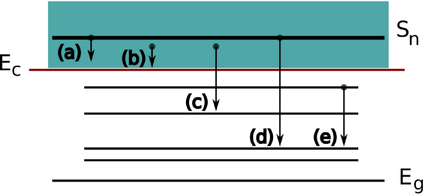
The classification of individual deexcitations coming from the cascade has become standard and is useful for relating the properties of the cascade to the nuclear structure. In addition, this classification aides in Monte Carlo codes to generate specific cascade realizations. Generally, a critical energy $E_{c}$ is chosen below the neutron separation energy such that nuclear levels below are treated individually with their appropriate properties and levels between this energy and the neutron separation energy are treated statistically. This breaks all released gamma rays into several categories as displayed in Fig. 1: (a) primary to continuum; (b) continuum to continuum; (c) continuum to discrete; (d) primary to discrete; and (e) discrete to discrete.

Figure 1: (Color online) The typical classification for capture cascade gamma rays. Horizontal lines are various energy demarcations with $S_{n}$ representing the neutron separation energy, $E_{g}$ representing the ground-state energy, and $E_{c}$ representing the (arbitrary) cut off between discrete and continuum states. Transitions are denoted by arrows and belong to one of five categories: (a) primary gammas with a final state in the continuum; (b) secondary gammas within the continuum; (c) secondary gammas from a continuum state to a discrete state; (d) primary gammas with a discrete final state; and (e) secondary gammas between two discrete states.

In our treatment of silicon here we will take $E_{c}\simeq S_{n}$, that is, we will treat all cascades as dicrete. This treatment may be difficult to implement for heavy nuclei as this approximation is most accurate for nuclei with low masses. Thus far, however, we have successfully treated 27% of germanium cascades in this fashion and are continuing to test this treatment on the remaining 73%.

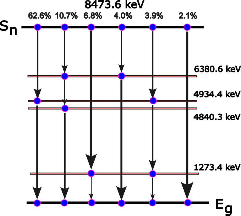
In PGAA measurements, it is easy to extract the prevalence of a specific gamma ray in the final state per 100 captures. We prefer the slightly different organization of giving the probability of a given cascade path. The key publication we use to sort out the cascade probabilities is the paper of Raman Raman et al. (1992). Figure 2 shows the cascade paths of the six most probable cascades for a natural silicon composition. The cascades shown there account for approximately 90% of the total cascades. Some of the gamma rays appear in multiple cascades so it is clear that the probability to find a specific gamma ray after capture — as is often measured — is not quite the same information as the cascade probabilities that we have compiled.

Figure 2: (Color online) A diagram of the six most prevalent cascades of natural silicon. All of the cascades start with the capture of approximately thermal neutrons on the nucleus ²⁸Si at the neutron separation energy of the final nuclear state, ²⁹Si.

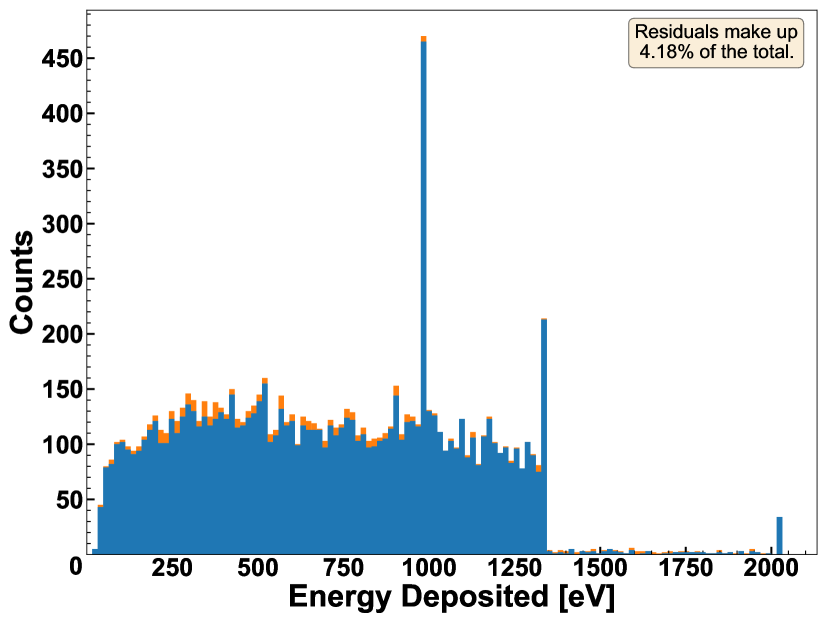
In our reorganization of this typical capture information, we have extracted the specific cascades which account for 95.63% of the total captures. This information is shown in Table 1 and is enough to construct an accurate model of the NRs left behind by capturing thermal neutrons. Figure 3 visualizes the effect the missing cascades have on the full spectrum of energy deposition. We have also gathered in the table the half-lives of each intermediate level where data are available and have otherwise used the Weisskopf estimates Weisskopf (1951).

Figure 3: (Color online) A stacked histogram of energy deposits simulated by nrCascadeSim v1.5.0 Villano et al. (2022b). On the bottom in blue (dark) are the cascades listed in Table 1. Stacked on top of them in orange (light) are the remaining cascades.

Level lifetimes are important for our modeling because even in a dense (crystalline) matrix the intermediate-state half-lives are typically short enough to allow for a “decay in flight.” In other words, it is not a good approximation to assume that the excited nucleus in each intermediate level stops before the subsequent decay. This has important implications for our kinematics calculations later. We select a specific cascade path to model so we should technically be using a level lifetime corrected for other branchings. The differences are small — probably well below 10% — because most of our highly-probable cascades involve the dominant decay branch.

Isotope	Probability (%)	Energy levels (keV)	Half-lives (fs)
28Si	62.6	4934.39	0.84
28Si	10.7	6380.58, 4840.34	0.36, 3.5
28Si	6.8	1273.37	291.0
28Si	4.0	6380.58	0.36
28Si	3.9	4934.39, 1273.37	0.84, 291.0
28Si	2.1	$\cdots$	$\cdots$
29Si	1.5	6744.10	14
30Si	1.4	3532.9, 752.20	6.9, 530
29Si	1.2	7507.8, 2235.30	24, 215
29Si	0.4	8163.20	w(E1)[0.0019]
30Si	0.4	5281.4, 752.20	w(E1)[0.0069], 530
29Si	0.3	$\cdots$	$\cdots$
30Si	0.3	4382.4, 752.20	w(E1)[0.012], 530
30Si	0.03	$\cdots$	$\cdots$

Table 1: A table displaying the probability of each cascade. This table includes only the cascades used for our model. The isotope listed is the isotope on which the neutron captures; the energy levels and half-lives are therefore for an isotope of silicon with one more neutron. A half-life entry in [brackets] preceeded by w(E1) specifies that the half-life is unknown and the Weisskopf estimate for an electric dipole transition was used Weisskopf (1951).

The possibility of “decay in flight” also makes a calculation of the slowing-down of recoiling atoms germane to our modeling. Here, we use a constant acceleration to model this slowing down, consistent with the average stopping power derived by Lindhard Lindhard et al. (1963). Lindhard used a generic Thomas-Fermi potential for all ions, and the result was a stopping power (acceleration) $S$ that depended on energy for slow nuclei between about 100 eV and 1 keV. We use the average of that curve between those energies, $S=0.1$.

To estimate a rough impact of the use of an average stopping power, we compared data generated by nrCascadeSim v1.5.0 Villano et al. (2022b) with stopping powers of $S=0.05$ and $S=0.15$ and found the average difference to be $22\%$, with the 984 eV peak differing by $97\%$. The qualitative differences between the $S=0.05$ and $S=0.15$ stopping powers are minimal; the greater stopping power results in larger peaks associated with full stops before decay, but covers the same region with similar distributions for nonpeak events. While peaks are taller for the greater stopping power, they are still noticeable in both cases. This indicates that one very sensitive measure of the average stopping power in our energy spectrum is the ratio of the tallest peak to the flat region.

III Two-Step Cascades

For cascades which emit either one or two gamma rays (one- or two-step cascades), we were able to analytically construct the distribution of total NR energies. This distribution will be what is observed in a detector that experiences a neutron capture when all the gamma rays leave without energy deposit.

For one-step cascades, a single gamma is emitted back-to-back with the NR. The gamma energy in this case is approximately the neutron separation energy, $E_{\gamma}\simeq S_{n}$. The NR energy, $T$, is given approximately by

$$T\simeq\frac{S_{n}^{2}}{2M_{A}}.$$ (1)

where $M_{A}$ is the mass of the recoiling nucleus.

The two-step cascades are considerably more complex because of the possibility of decay in flight. We work with a separation of the nuclear energy deposits into the first and second steps like: $D_{t}=D_{1}+D_{2}$. $D_{t}$ is the total deposited energy by the NRs. $D_{1}$ and $D_{2}$ are the energies deposited before the intermediate decay and after the intermediate decay respectively. The two other key variables we will use are the decay time, $t$, and the center-of-mass angle for the decay, $\beta_{\mathrm{cm}}$. The energy deposits are deterministic functions of the decay times and angles, both of which are in turn probabilistic random variables.

The decay time represents how long it takes for the (instantaneously generated) intermediate state to decay to the ground state and is exponentially distributed with the probability density function (PDF) in Eq. (2). The cosine of $\beta_{\mathrm{cm}}$ is assumed to be uniformly distributed over $(-1,1)$ in the center-of-mass frame for the decay. The possible correlation between gamma directions is mostly erased by the interaction of the excited state with the lattice. We estimate that around 8$\times$10^-4% of the time there could be a cascade that emits two gammas nearly simultaneously — in that case any correlation will remain but has not been accounted for here,

$$f(t)=\frac{\ln{2}}{t_{1/2}}\exp\left[-t\frac{\ln{2}}{t_{1/2}}\right],$$ (2)

The quantity $D_{1}$ can be expressed as a simple function of $t$, given that the recoiling nucleus slows down with a constant (negative) acceleration, $a$,

$$D_{1}(t)=T_{1}-\frac{M_{A}^{\ast}(v_{0}-at)^{2}}{2},$$ (3)

where $T_{1}$ is the total kinetic energy the intermediate state receives from the first gamma recoil, $M_{A}^{\ast}$ is the mass of the intermediate state, and $v_{0}=(2T_{1}/M_{A}^{\ast})^{1/2}$ is the initial velocity.

Modeling the process with a fixed acceleration gives a unique stopping time, $t_{s}$. The distribution of $D_{1}$ has a singular value of $T_{1}$ if $t>t_{s}$, but the PDF for $t<t_{s}$ depends on Eq. (2) with a change of variables to the $D_{1}$ of Eq. (3). The result is

$$g(D_{1}) =\begin{cases}g^{0}(D_{1})+\exp{\left[-\ln{2}\frac{t_{s}}{t_{1/2}}\right]}\delta(D_{1}-T_{1})&;D_{1}\leq T_{1}\\ 0&;D_{1}>T_{1}\end{cases}$$ (4)

$$g^{0}(D_{1}) =\frac{\ln{2}}{|a|t_{1/2}\sqrt{2M_{A}^{\ast}(T_{1}-D_{1})}}\exp{\left[-\ln{2}\frac{v_{0}-\sqrt{2(T_{1}-D_{1})/M_{A}^{\ast}}}{|a|t_{1/2}}\right]},$$

where $\delta(\cdot)$ is the Dirac delta function.

The PDF of $D_{2}$ is clearly dependent on $D_{1}$ because the value of $D_{2}$ depends on $t$ which is deterministically related to $D_{1}$. We deal with this by using the joint PDF of $D_{1}$ and $D_{2}$, $g(D_{1},D_{2})$. The PDF for $D_{2}$ can then be obtained by integrating the joint PDF over all $D_{1}$.

To obtain the joint distribution $g(D_{1},D_{2})$ we use a basic relationship from conditional probability,

$$g(D_{1},D_{2})=h(D_{2}|D_{1})g(D_{1}).$$ (5)

The PDF $h(D_{2}|D_{1})$ is the PDF of $D_{2}$ given a specific value of $D_{1}$. The function $h$ is not challenging to obtain because the only relevant random variable is $\beta_{\mathrm{cm}}$– $t$ is fixed because $D_{1}$ is fixed. We can then think of $D_{2}$ as a deterministic function of $D_{1}$ and $\beta{\mathrm{cm}}$ like $D_{2}(t(D_{1}),\beta_{\mathrm{cm}})$.

To obtain the function $h$ we note that whatever kinetic energy the final nucleus has after the intermediate decay will be the deposited energy . We calculated bounds on this kinetic energy, $T_{2}$, given the value of $\beta_{\mathrm{cm}}$,

$$\begin{split}T_{2}=\frac{\Delta^{2}}{2M_{A}}&\left[\frac{2M_{A}(T_{1}-D_{1})}{\Delta^{2}}\right.\\ &\left.+2\sqrt{\frac{2M_{A}(T_{1}-D_{1})}{\Delta^{2}}}\cos{\beta_{\mathrm{cm}}}+1\right],\end{split}$$ (6)

where $\Delta$ is the difference between the intermediate state energy and the ground state. The value of $\cos{\beta_{\mathrm{cm}}}$ is between -1 and 1, so this gives a clear minimum and maximum for this kinetic energy. An alternate form for the kinetic energy $T_{2}$ is given in Appendix A. The total energy deposited can be zero if and only if the decay is immediate and $\Delta$ is exactly halfway between the ground state and the neutron separation energy $S_{n}$. The function $h$ is then

$$h(D_{2}|D_{1})=\\ \begin{cases}\frac{1}{2\Delta}\sqrt{\frac{M_{A}}{2}\frac{1}{T_{1}-D_{1}}}&;T_{2,\mathrm{min}}\leq D_{2}\leq T_{2,\mathrm{max}}\\ 0&;\mathrm{otherwise}\end{cases}\\$$ (7)

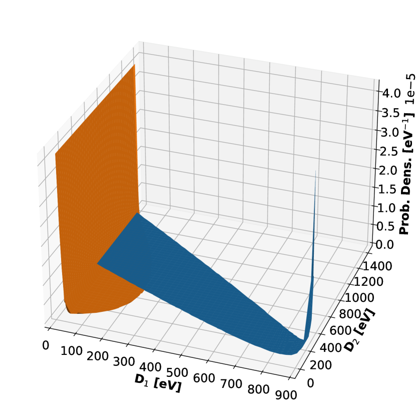
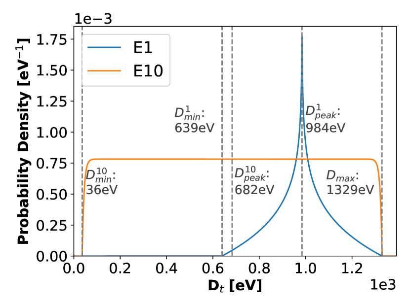
Using Eq. (7) we constructed the joint distribution from Eq. (5). The joint distribution is plotted in Fig. 4 for two cascades — one (orange) with a very fast intermediate decay and another (blue) with a slower intermediate decay. The spike shown in the slow distribution is a two-dimensional Dirac delta function that corresponds to the situation when the intermediate recoil stops before the subsequent decay. In that case the values of $D_{1}$ and $D_{2}$ are fixed and are the values you would expect from at-rest one-gamma decay of each excited nuclear state. The fast intermediate decay produces a behavior where $D_{1}$ tends to be lower and increases toward zero.

Figure 4: (Color online) The two-dimensional joint PDF from Eq. (5). $D_{1}$ and $D_{2}$ are the energies deposited from the first and second cascade step respectively. The darker (blue) surface is for a two-step cascade stopping at the first excited state of ²⁹Si; the lighter (orange) surface is for a two-step cascade stopping at the (tenth) excited state of ²⁹Si — the most likely cascade.

With the joint distribution specified, the distribution of the total energy deposit, $D_{t}$ is obtained by the following integral:

$$p(D_{t})=\int_{D_{1}}g(D_{1},D_{t}-D_{1})dD_{1}.$$ (8)

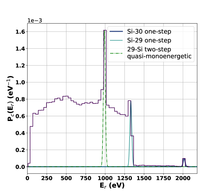
The total distribution for $D_{t}$ is plotted in Fig. 5 for both example cascades. Once again the “spike” in the slow cascade corresponds to the case where the intermediate recoil stops before the subsequent decay — that results in a fixed total energy deposited. This spike is proportional to the Dirac delta function, and so cannot be shown on the correct scale. However, it is easy to see the $D_{t}$ value for the spike and it must account for the remaining probability after removing the integral of the plotted distribution. In the fast cascade most remnants of the monoenergetic “spike” are gone and the total energy is nearly uniform between two fixed bounds.

Figure 5: (Color online) The PDF of the total deposited energy from nuclear recoils, $D_{t}$, for this two-step cascade. E1 indicates the intermediate level being the first excited state of ²⁹Si; E10 indicates the intermediate level being tenth excited state of ²⁹Si — the most likely cascade for Si.

IV Monte Carlo Approach

For cascades with more than two steps we have not worked out the analytical distributions as we have in Sec. III. For these many step cascades we use a Monte Carlo approach that allows us to include arbitrarily many steps in the sequence. The main limitation is that we compute one thermal neutron capture realization at a time so that it might be prohibitive to produce a PDF with sufficient smoothness (high statistics) for cascades with small overall likelihood. On the other hand, those cascades represent only a small change to an experimental spectrum Villano et al. (2022a).

Using the information from Table 1, these steps are followed to generate one Monte Carlo capture event:

1. Select a cascade with a probability based on the prevalence of that specific deexcitation path.

2. Randomly select a decay time for the first intermediate state based on an exponential distribution with the appropriate lifetime. This variable is $t$ from the two-step calculation.

3. Calculate the first energy deposit $D_{1}$ based on the decay time and the stopping acceleration. This is the slowing-down energy deposited in time $t$.

4. Adjust the kinetic energy of the recoil based on the kinematics of in-flight decay. This adjustment is based on the center-of-mass angle of the emitted gamma, $\beta_{\mathrm{cm}}$ from the two-step calculation.

5. Repeat steps 2–4 for each intermediate level.

The result of this procedure is a set of energy deposits $\{D_{i}\}$ with the same number of elements as gamma rays emitted. The $D_{i}$s are saved and may be summed to obtain the total deposited energy. The emitted gamma ray energies for each step are saved alongside the $D_{i}$s. These steps are implemented in our public code Villano et al. (2022b).

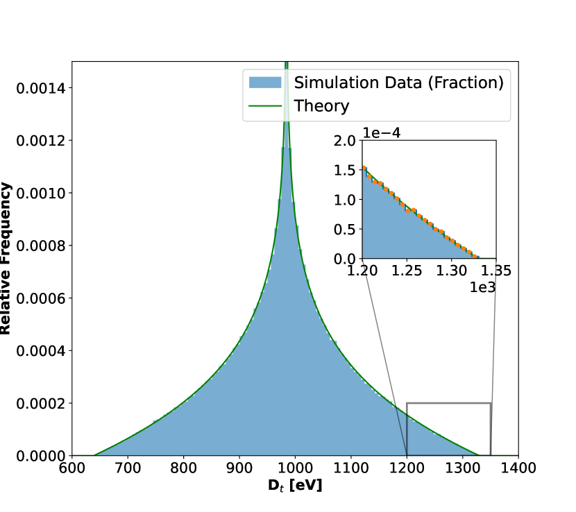
Figure 6 shows how the analytical calculation for the deposited energy of a two-step cascade compares to our Monte Carlo procedure. The two are an excellent match and the reduced $\chi^{2}$ statistic is 1.02.

Figure 6: (Color online) A comparison of the analytical PDF for the two-step cascade (see Sec. III) with that of the Monte Carlo procedure. The histogram is the PDF derived from many events generated by the Monte Carlo procedure.

The full spectrum from all the cascades in Table 1 is shown in Fig. 7 with a 10 eV nominal resolution applied. The sharpest peaks come from the direct-to-ground transitions of ²⁹Si and ³⁰Si and the 6.8% two-step transition. In the two-step transition there is a sizeable probability of having the first NR stop before the subsequent decay — it is a quasimonoenergetic transition for this reason.

Figure 7: (Color online) The complete silicon capture spectrum using the data from Table 1. 95.63% of all cascades are taken into account here. A nominal 10 eV resolution has been applied.

When we use these spectra we account for the events that will be distorted by energy deposits from the exiting gammas Villano et al. (2022a). This is sometimes done by estimating what fraction of cascades have gammas that escape (around 90% for a cylindrical silicon detector of diameter 100 mm and thickness 30 mm). Other times we use a particle transport code like Geant4 to find exactly which cascade realizations have exiting gamma interactions. When using materials that are more electron dense than silicon the fraction of interactions from exiting gammas increases. It is typically true that those events that have interactions from exiting (high-energy) gammas will be removed from the low energy range completely — they produce little contamination of the capture-induced NR “signal.”

The Geant4 particle transport code gets different results for the resulting NR spectra from the capture process with silicon, germanium, and neon Villano et al. (2022b). The results for silicon are the closest but still have significant differences that may be experimentally relevant to dark matter and CENS studies. The most recent version of Geant4 that was compared to our spectral results is v10.7.3 and comparisons are stored with our open-source code Villano et al. (2022b).

V Uses for Dark Matter and CENS

Our major goals in understanding the neutron capture induced nuclear recoil spectra are (a) to use these nuclear recoil events to enhance our understanding of low-energy nuclear recoils in solids — to provide excellent low-energy calibrations and (b) to compute the experimental backgrounds for dark matter and CENS searches.

In silicon and other materials there has not been consensus on how much ionization nuclear recoils produce at low recoil energies. Typically, our theoretical guidance in the field comes from the early Lindhard paper Lindhard et al. (1963) and associated work. On the other hand, measurements down to the 100 eV range seem like they may deviate from those predictions and be marginally consistent or inconsistent with each other Izraelevitch et al. (2017); Chavarria et al. (2016); Villano et al. (2022a).

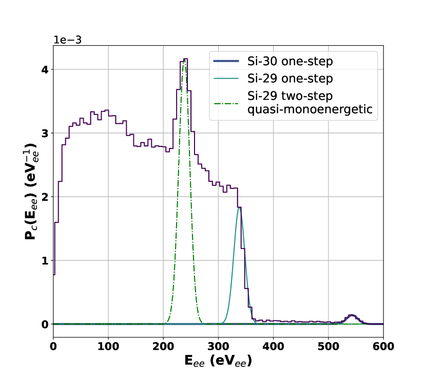
Exploring the detector response to NRs at low energies is therefore prudent and thermal neutron induced captures provide an excellent venue for this — as pointed out by the CRAB Collaboration Thulliez et al. (2021) and others working with xenon for dark matter Amarasinghe et al. (2022). The key features for thermal neutron induced captures are shown in Fig. 8. In that figure a nominal Lindhard ionization yield Lindhard et al. (1963) is applied to the result shown in Fig. 7.

Figure 8: (Color online) The NR capture spectrum corresponding to events that are resulting from neutron-capture. The three Gaussian peaks shown outline the particular cascades that have sharp signatures. The horizontal scale is in electron-equivalent energy (eV_ee) which quantifies the amount of charge produced rather than the true recoil energy of the NR (which is higher). 95.63% of all cascades are modeled using the data from Table 1. A nominal 10 eV_ee resolution has been applied.

Calibrations using thermal neutron induced captures are superior to other styles of calibrations that have been used: direct elastic neutron scattering Gerbier et al. (1990), photoneutron sources Albakry et al. (2022); Scholz et al. (2016), and ²⁵²Cf sources Agnese et al. (2018a). Figure 8 shows that the spectrum has sharp mono-energetic features that are lacking in wide-band photoneutron or ²⁵²Cf sources. The spectrum extends down well below 100 eV which is probably near the limit of elastic scattering sources. Using this technique is also feasible in situ because any neutron source will elevate the thermal neutron flux during its deployment. Finally, if there is a case where exiting gammas can be measured in coincidence, the direct-to-ground transitions provide directionally tagged nuclear recoils. This would lead to a heretofore unavailable NR directionality calibration, as pointed out in Thulliez et al. (2021).

A large enough thermal neutron flux could lead to meaningful backgrounds for low-mass dark matter searches or CENS measurements. The thermal neutron flux is typically not measured directly in many experiments because of the difficulty in doing so. One measurement that does exist for CENS is from the MINER collaboration Agnolet et al. (2017) and is several orders of magnitude higher than the accepted sea level environmental value, 4 cm^-2 hr^-1 Dirk et al. (2003). We have previously shown the effect of thermal neutrons on CENS measurements in detail Biffl et al. (2022).

The SuperCDMS Soudan thermal neutron flux can be estimated from the germanium activation lines Agnese et al. (2019) and is $\lesssim$ 7.2$\times$10^-2 cm^-2 hr^-1.

Figure 9: (Color online) Comparison of the thermal neutron capture induced NR spectrum in silicon with expected dark matter and CENS signals in line with currently available data.

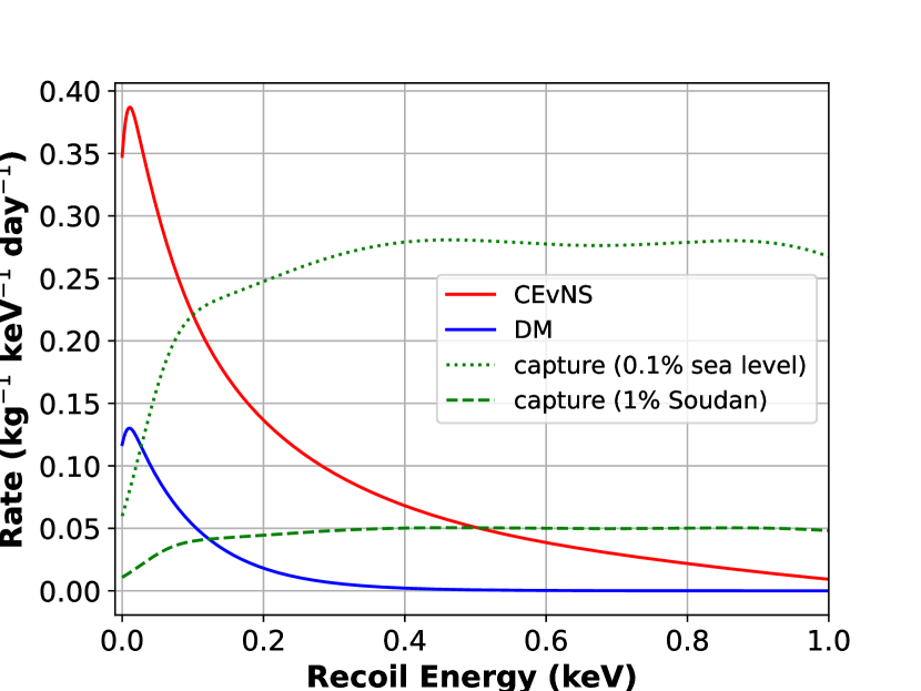
Figure 9 shows the comparison of the thermal neutron induced NR spectra at the estimated flux levels without shielding with the dark matter and CENS spectra. The capture cross section is assumed to be 0.171 barns, from 2003 measurements at Brookhaven National Lab Mughabghab (2003) (this value is also used in the EGAF (Evaluated Gamma Activation File) database Firestone et al. (2005)). This value is about 4% higher than the value given by evaluations a few years earlier at Los Alamos National Lab that are used in ENDF and the JENDL 5 database Iwamoto et al. (2023) and the cross section measurements made by Raman Raman et al. (1992).

For a CENS experiment with a 1 MW reactor at a distance of 8 m we arbitrarily compared a thermal neutron flux of 0.1% of the sea level value. We have used the Mueller spectrum for the reactor anti-neutrinos Mueller et al. (2011). The detector resolution function is assumed to have a 10 eV baseline that rises to 30 eV at a recoil energy of 25 eV. We use this form for the energy-varying resolution: $\sqrt{\sigma_{0}^{2}+AE_{r}}$; $E_{r}$ is the recoil energy and $\sigma_{0}$ and $A$ are constants.

For the dark matter comparisons in Fig. 9 we used a 1 GeV mass dark matter particle with a cross section just below the limit produced in recent SuperCDMS work Agnese et al. (2019, 2018b).

Figure 9 shows that both for dark matter searches and CENS the spectral overlap of thermal neutron capture induced NRs can interfere with measurements especially in cases where the detector baseline resolutions are larger than 10 eV — true for all but the best modern detectors.

VI Conclusion

We have carefully derived and simulated the spectrum of NRs following thermal neutron captures in silicon. The spectra do not match the contemporary Geant4 particle transport code, indicating the details of decay-in-flight and atomic slowing-down are poorly modeled.

The level of thermal neutron fluxes that may be present in underground laboratories (mostly from radiogenic sources in deep labs) is comparable to the contemporary rate limits on dark matter scattering. Furthermore, in the CENS venue the thermal neutron capture background could also play an important role due to the proximity of some experiments to neutron-generating reactors Colaresi et al. (2022); Ang et al. (2021). In both of these situations the authors recommend studies of the thermal neutron flux levels and taking the thermal neutron capture background into account during data analysis.

Appendix A Another perspective on equations

In Sec. III, we give several equations that are constructed from the perspective of simulation. Below are the derivations, from the equations in Sec. III, of equivalent forms that give a more conceptual perspective.

We use the following substitutions. Let $v_{1}=(2(T_{1}-D_{1})/M_{A}^{*})^{1/2}$ be the velocity just before the second gamma’s emission, $v_{CM}=\Delta/M_{A}$ be the velocity just after emission in the center-of-mass frame, and $E_{1}=\frac{1}{2}M_{A}^{*}v_{1}^{2}$ and $E_{C}M=\frac{1}{2}M_{A}v_{CM}^{2}$ be the associated kinetic energies.

First, we will reorganize $g^{0}(D_{1})$ from Eq. (4):

$$g^{0}(D_{1}) =\frac{v_{1}\ln 2}{v_{1}|a|t_{1/2}M_{A}^{*}\sqrt{2(T_{1}-D_{1})/M_{A}^{*}}}\exp{\left(-\ln 2\frac{v_{0}-v_{1}}{|a|t_{1/2}}\right)}$$ (9)

$$=\frac{v_{1}\ln 2}{|a|t_{1/2}M_{A}^{*}v_{1}^{2}}\exp{\left(-\ln 2\frac{v_{0}-v_{1}}{|a|t_{1/2}}\right)}$$

$$=\frac{\ln 2}{2E_{1}}\frac{v_{1}}{|a|t_{1/2}}\exp\left(-\ln 2\frac{v_{0}-v_{1}}{|a|t_{1/2}}\right).$$

Next, we reorganize $T_{2}$, given by Eq. (6):

$$T_{2} =\frac{1}{2}M_{A}\frac{\Delta^{2}}{M_{A}^{2}}\left[\frac{M_{A}^{2}M_{A}^{*}\sqrt{2(T_{1}-D_{1})/M_{A}^{*}}^{2}}{M_{A}\Delta^{2}}+2\sqrt{M_{A}M_{A}^{*}}\sqrt{\frac{2(T_{1}-D_{1})/M_{A}}{\Delta^{2}}}\cos\beta_{CM}+1\right]$$ (10)

$$=\frac{1}{2}M_{A}v_{CM}^{2}\left[\frac{M_{A}^{*}v_{1}^{2}}{M_{A}v_{CM}^{2}}+2\sqrt{\frac{M_{A}^{*}v_{1}^{2}}{M_{A}v_{CM}^{2}}}\cos\beta_{CM}+1\right]$$

$$=E_{C}M\left[\frac{E_{1}}{E_{CM}}+2\sqrt{\frac{E_{1}}{E_{CM}}}\cos\beta_{CM}+1\right]$$

This new form for $T_{2}$ makes it clear that $T_{2}$ can reach zero when $E_{1}=E_{CM}$ and $\beta=\pi$.

Finally, we reorganize $h(D_{2}|D_{1})$ for the nonzero case, given by Eq. (7):

$$h(D_{2}|D_{1}) =\frac{M_{A}}{2M_{A}\Delta}\sqrt{\frac{1/M_{A}M_{A}^{*}}{2(T_{1}-D_{1})/M_{A}^{*}}}$$ (11)

$$=\frac{2}{4M_{A}v_{CM}}\sqrt{\frac{M_{A}}{M_{A}^{*}}}\frac{1}{v_{1}}$$

$$=\frac{2}{4M_{A}v_{CM}^{2}}\sqrt{\frac{M_{A}v_{CM}^{2}}{M_{A}^{*}v_{1}^{2}}}$$

$$=\frac{1}{4E_{CM}}\sqrt{\frac{E_{CM}}{E_{1}}}$$