Nonlinear Balanced Truncation:
Part 2—Model Reduction on Manifolds

Abstract

Nonlinear balanced truncation is a model order reduction technique that reduces the dimension of nonlinear systems in a manner that accounts for either open- or closed-loop observability and controllability aspects of the system. Two computational challenges have so far prevented its deployment on large-scale systems: (a) the energy functions required for characterization of controllability and observability are solutions of high-dimensional Hamilton-Jacobi-(Bellman) equations, which have been computationally intractable and (b) the transformations to construct the reduced-order models (ROMs) are potentially ill-conditioned and the resulting ROMs are difficult to simulate on the nonlinear balanced manifolds. Part 1 of this two-part article (​​ [30]) addressed challenge (a) via a scalable tensor-based method to solve for polynomial approximations of the open- and closed-loop energy functions. This article, (Part 2), addresses challenge (b) by presenting a novel and scalable method to reduce the dimensionality of the full-order model via model reduction on polynomially-nonlinear balanced manifolds. The associated nonlinear state transformation simultaneously “diagonalizes” relevant energy functions in the new coordinates. Since this nonlinear balancing transformation can be ill-conditioned and expensive to evaluate, inspired by the linear case we develop a computationally efficient balance-and-reduce strategy, resulting in a scalable and better conditioned truncated transformation to produce balanced ROMs. The algorithm is demonstrated on a semi-discretized partial differential equation, namely Burgers equation, which illustrates that higher-degree transformations can improve the accuracy of ROM outputs.

Reduced-order modeling, balanced truncation, nonlinear manifolds, Hamilton-Jacobi-Bellman equation, nonlinear control-affine systems.

1 Introduction

Simulation of large-scale nonlinear dynamical systems can be time-consuming and resource-intensive. It is a frequent bottleneck when these simulations are used for real-time, model-based control. Reduced-order models (ROMs) provide an attractive solution to this problem by approximating dynamical systems (and their relevant system-theoretic properties) in a much lower dimensional state space; see, e.g., [3, 2, 6, 53, 48, 8] for a general overview. These ROMs then allow for the design of low-dimensional controllers and filters.

Balanced truncation model reduction, as pioneered by Moore [37] and Mullis and Roberts [38] for linear time-invariant (LTI) systems, provides an elegant approach to the model reduction problem for open-loop settings. The approach uses the controllability and observability energies of a system to determine those states that have the most relative importance. If a state requires a large amount of input energy to be reached and also has minimal effect on the output, then the reduced model would neglect that state without a significant impact on the input-output behavior of the system. Extensions of this concept to closed-loop LTI systems led to the LQG balancing [51, 28] and $\mathcal{H}_{\infty}$ balancing concepts [39]. Several variants for different formulations of the LTI system and different reduced-model outcomes exist, such as stochastic balancing [15, 25], bounded real balancing [41], positive real balancing [15, 40], and frequency-weighted balancing [18]; see also the surveys [26, 5]. The interest in balancing methods for LTI systems in the 1980s stimulated research in computational methods for solving large-scale Lyapunov or Riccati-type algebraic matrix equations that yielded low-rank solvers [9, 49] and doubling methods [35] that can solve these matrix equations for millions of states.

For nonlinear large-scale systems, the theory is largely developed, yet computationally scalable approaches and efficient ROM development remain open problems. The theoretical foundation for balanced truncation of nonlinear open-loop systems proposed by Scherpen [45] defines input and output energy functions and shows that they can be computed as solutions to Hamilton-Jacobi (HJ) partial differential equations (PDEs). Theoretical extensions of [45] to the closed-loop setting, such as Hamilton-Jacobi-Bellman (HJB) balancing [47] and $\mathcal{H}_{\infty}$ balancing [46] have also been proposed for nonlinear systems, which can be unstable. Aside from the need for computing solutions of HJ(B) equations, nonlinear balancing requires a nonlinear transformation whereas balancing for LTI systems requires a linear change of variables. While reduced models obtained through the original nonlinear balancing framework [45] were quickly shown to be non-unique [23], a slightly altered transformation suggested in [20] resolved this issue, resulting in uniquely determined reduced-order models. Krener [31] suggested a different balancing strategy that applies the balancing to each degree of the polynomial approximations of the energy functions separately. The full nonlinear balance-then-reduce approaches first compute the balancing transformation in the high-dimensional space, and subsequently reduce the model dimension, see [45, 47, 46, 21, 43]. However, in the linear case, balance-then-reduce approaches have been shown to be ill-conditioned due the need to invert small Hankel singular values [2]. In sum, the nonlinear transformation is difficult to compute—reducing the efficiency of the nonlinear ROM—and can be ill-conditioned as well. Lastly, the development of an error bound similar to the linear case (in terms of neglected Hankel singular values) remains an open problem.

Other methods for reducing the dimensionality of the FOM via balancing have been proposed that avoid the computation of the fully nonlinear energy function. Generally, these methods compute a quadratic energy function that then leads to linear subspace reduction. For instance, [24, 7] derive algebraic Gramians for the nonlinear system and propose a linear coordinate transform. The authors in [14] combined Carleman bilinearization with a balancing method to approximately balance weakly nonlinear systems. Empirical Gramians for nonlinear systems can also be used [33] and also lead to linear subspace reduction. Lastly, a method for approximating the nonlinear balanced truncation reduction map via reproducing kernel Hilbert spaces (a machine learning-based, data-driven technique) has been proposed in [11], and applied to two- and seven-dimensional ODE examples. The idea is to embed the nonlinear dynamical system into a high (or infinite) dimensional Reproducing Kernel Hilbert Space (RKHS). There, linear theory can be applied. Then, the authors learn mappings from the high dimensional RKHS to the balanced finite dimensional system and demonstrate their results on 2d and 7d ODE examples. There also exist related methods that balance different characteristics of the problem (not the aforementioned nonlinear energy functions), such as flow balancing [52], incremental balancing [10], dynamic balancing [44]. These methods are only loosely connected to the nonlinear Hankel operator and the energy functions [29]. Moreover, incremental balancing is restricted to only odd functions on the right-hand-side of the dynamical systems. Another type of balancing, called differential balancing [29], has been developed with a connection to the nonlinear Hankel operator. This method requires solving linear time-dependent matrix inequalities (extensions of Lyapunov inequalities) and is therefore focused on open-loop systems.

In this two-part article, we propose a scalable and computationally efficient nonlinear balanced truncation approach via nonlinear energy functions that works for both closed- and open-loop systems. Such a method is currently lacking for medium- and large-scale systems. In Part 1 of this article, [30], we (i) propose a unifying framework to the open- and closed-loop nonlinear balancing problem by considering Taylor-series-based approaches to solve a class of parametrized HJB equations; (ii) derive the explicit tensor structure for the coefficients of the polynomial expansion which allows our numerical methods to scale up to thousands of state variables; (iii) provide large-scale numerical examples, a scalability analysis, and open-access software for all algorithms.

There are three main contributions of this article (Part 2). First, we present a scalable Taylor-series-based strategy that is implemented in open-access software (the NLbalancing repository [1]) for computing the nonlinear state transformations and singular value functions. We then derive the nonlinearly balanced models. The nonlinear state transformation simultaneously “diagonalizes” the open- and closed-loop energy functions in the new coordinates. However, this nonlinear balancing transformation can be ill-conditioned (which also occurs in the LTI case) and is expensive to evaluate. Second, we thus develop a computationally efficient balance-and-reduce strategy that reduces the dimensional of the full-order model (FOM) via model reduction on nonlinear manifolds. The strategy addresses the ill-conditioning problem in the full nonlinear transformation and allows for efficient nonlinear ROM construction. Third, we present nonlinear balanced ROMs for a semi-discretized PDE of Burgers-type, where we investigate the impact of the degree of the nonlinear transformation on the ROM input-output quality and illustrate the behavior of the singular value functions. We highlight that the work herein does not assume a specific form of the dynamical system: the transformation merely balances two polynomial energy functions and produces a nonlinear mapping that can be applied to any nonlinear system.

This article is organized as follows. Section 2 briefly reviews background material on energy functions for nonlinear systems. Section 3 presents our first key contribution, a scalable strategy for computing the nonlinear basis transformations and the singular value functions. We also present the nonlinearly balanced models in that section. Section 4 presents our second key contribution, a modified and scalable method to obtain a balanced nonlinear ROM that addresses the ill-conditioning problem in the full nonlinear transformation and allows for more efficient nonlinear ROM evaluation. Section 5 presents numerical results for the nonlinear ROMs for the semi-discretized Burgers equation. Lastly, Section 6 offers conclusions and an outlook toward future work.

2 Energy functions for nonlinear balancing

This section briefly reviews the unifying concept of the $\mathcal{H}_{\infty}$ energy functions for nonlinear control-affine dynamical systems, see Part 1 of this article ([30]) for more details. Consider the finite-dimensional system

$$\dot{\mathbf{x}}(t) =\mathbf{f}(\mathbf{x}(t))+\mathbf{g}(\mathbf{x}(t))\mathbf{u}(t),$$ (1)

$$\mathbf{y}(t) =\mathbf{h}(\mathbf{x}(t)),$$ (2)

where $t$ denotes time, $\mathbf{x}(t)\in\mathbb{R}^{n}$ is the state, $\mathbf{u}(t)\in\mathbb{R}^{m}$ is a time-dependent input vector, $\mathbf{g}:\mathbb{R}^{n}\mapsto\mathbb{R}^{n\times m}$ encodes the actuation mechanism, $\mathbf{y}(t)\in\mathbb{R}^{p}$ is the output vector measured by the function $\mathbf{h}:\mathbb{R}^{n}\mapsto\mathbb{R}^{p}$, the nonlinear drift term is $\mathbf{f}:\mathbb{R}^{n}\mapsto\mathbb{R}^{n}$, and $\mathbf{x}=\mathbf{0}$ is an isolated equilibrium point for $\mathbf{u}=\mathbf{0}$. For the system (1)-(2), the $\mathcal{H}_{\infty}$ past energy in the state $\mathbf{x}_{0}$ is defined, for $0<\gamma$, $\gamma\neq 1$, as

$$\mathcal{E}_{\gamma}^{-}(\mathbf{x}_{0}):=\min_{\begin{subarray}{c}\mathbf{u}\in L_{2}(-\infty,0]\\ \mathbf{x}(-\infty)=\mathbf{0},\\ \mathbf{x}(0)=\mathbf{x}_{0}\end{subarray}}\ \frac{1}{2}\int\displaylimits_{-\infty}^{0}(1-\gamma^{-2})\|\mathbf{y}(t)\|^{2}+\|\mathbf{u}(t)\|^{2}{\rm{d}}t.$$ (3)

Furthermore, the $\mathcal{H}_{\infty}$ future energy in the state $\mathbf{x}_{0}$ is defined, for $0<\gamma<1$ as

$$\mathcal{E}_{\gamma}^{+}(\mathbf{x}_{0}):=\max_{\begin{subarray}{c}\mathbf{u}\in L_{2}[0,\infty)\\ \mathbf{x}(0)=\mathbf{x}_{0},\\ \mathbf{x}(\infty)=\mathbf{0}\end{subarray}}\ \frac{1}{2}\int\displaylimits_{0}^{\infty}\|\mathbf{y}(t)\|^{2}+\frac{\|\mathbf{u}(t)\|^{2}}{1-\gamma^{-2}}{\rm{d}}t,$$ (4)

and for $\gamma>1$, as

$$\mathcal{E}_{\gamma}^{+}(\mathbf{x}_{0}):=\min_{\begin{subarray}{c}\mathbf{u}\in L_{2}[0,\infty)\\ \mathbf{x}(0)=\mathbf{x}_{0},\\ \mathbf{x}(\infty)=\mathbf{0}\end{subarray}}\ \frac{1}{2}\int\displaylimits_{0}^{\infty}\|\mathbf{y}(t)\|^{2}+\frac{\|\mathbf{u}(t)\|^{2}}{1-\gamma^{-2}}{\rm{d}}t.$$ (5)

The $\mathcal{H}_{\infty}$ energy functions can be computed via HJB PDEs, see Part 1 of this paper, [30, Sec. II], for more details. For LTI systems, these energy functions are quadratic in the state and can be computed by solving $\mathcal{H}_{\infty}$ algebraic Riccati equations.

Under the assumption that the energy functions exist and are smooth, the open-loop nonlinear energy functions $\mathcal{E}_{c}(\mathbf{x})$ and $\mathcal{E}_{o}(\mathbf{x})$ (see [30, Sec 2.5] can be obtained in the limit $\gamma\rightarrow 1$ of the $\mathcal{H}_{\infty}$ energy functions $\mathcal{E}_{\gamma}^{-}(\mathbf{x})$ and $\mathcal{E}_{\gamma}^{+}(\mathbf{x})$, i.e.,

$$\lim_{\gamma\rightarrow 1}\mathcal{E}_{\gamma}^{-}(\mathbf{x})=\mathcal{E}_{c}(\mathbf{x}),\quad\lim_{\gamma\rightarrow 1}\mathcal{E}_{\gamma}^{+}(\mathbf{x})=\mathcal{E}_{o}(\mathbf{x}).$$ (6)

In this article, we assume similar to [36] that the energy functions are polynomial (or are approximated as such), which allows us scalability in our approach to the model reduction process. In particular, we assume that the past energy function is represented in the form (or is approximated as)

$$\mathcal{E}_{\gamma}^{-}(\mathbf{x})\approx\frac{1}{2}\left(\mathbf{v}_{2}^{\top}\mathbf{x}^{\leavevmode\hbox to6.15pt{\vbox to6.15pt{\text{[drawing]}}}}+\mathbf{v}_{3}^{\top}\mathbf{x}^{\leavevmode\hbox to6.15pt{\vbox to6.15pt{\text{[drawing]}}}}+\cdots+\mathbf{v}_{d}^{\top}\mathbf{x}^{\leavevmode\hbox to6.53pt{\vbox to6.53pt{\text{[drawing]}}}}\right).$$ (7)

where $\mathbf{v}_{k}\in\mathbb{R}^{n^{k}}$ and $\mathbf{x}^{\leavevmode\hbox to6.44pt{\vbox to6.44pt{\text{[drawing]}}}}$ denotes the $k$-term Kronecker product of $\mathbf{x}$ defined as

$$\mathbf{x}^{\leavevmode\hbox to6.44pt{\vbox to6.44pt{\text{[drawing]}}}}:=\underbrace{\mathbf{x}\otimes\dots\otimes\mathbf{x}}_{k\ \text{times}}{\in\mathbb{R}^{n^{k}}}.$$ (8)

We also assume the future energy function $\mathcal{E}_{\gamma}^{+}(\mathbf{x})$ has the form (or is approximated as)

$$\mathcal{E}_{\gamma}^{+}(\mathbf{x}) \approx\frac{1}{2}\left(\mathbf{w}_{2}^{\top}\mathbf{x}^{\leavevmode\hbox to6.15pt{\vbox to6.15pt{\text{[drawing]}}}}+\mathbf{w}_{3}^{\top}\mathbf{x}^{\leavevmode\hbox to6.15pt{\vbox to6.15pt{\text{[drawing]}}}}+\dots+\mathbf{w}_{d}^{\top}\mathbf{x}^{\leavevmode\hbox to6.53pt{\vbox to6.53pt{\text{[drawing]}}}}\right),$$ (9)

where $\mathbf{w}_{k}\in\mathbb{R}^{n^{k}}$. To ensure a unique representation of the coefficients in (7) and (9), we assume that the polynomial representations of the energy functions have a symmetric representation as explained next.

Definition 1 (Symmetric Coefficients)

A monomial term with real coefficients $\mathbf{w}_{d}^{\top}\mathbf{x}^{\leavevmode\hbox to6.53pt{\vbox to6.53pt{\text{[drawing]}}}}$ has symmetric coefficients if it satisfies

$$\mathbf{w}_{d}^{\top}\left(\mathbf{a}_{1}\otimes\mathbf{a}_{2}\otimes\cdots\otimes\mathbf{a}_{d}\right)=\mathbf{w}_{d}^{\top}\left(\mathbf{a}_{i_{1}}\otimes\mathbf{a}_{i_{2}}\otimes\cdots\otimes\mathbf{a}_{i_{d}}\right),$$

where the indices $\{i_{k}\}_{k=1}^{d}$ are any permutation of $1,\ldots,d$.

Note that Algorithm 1 in Part 1 of this paper is designed to ensure symmetry in the computed coefficients. This symmetry definition generalizes the definition of symmetry from matrices to tensors. For example, requiring $\mathbf{w}_{2}^{\top}(\mathbf{a}\otimes\mathbf{b})=\mathbf{w}_{2}^{\top}(\mathbf{b}\otimes\mathbf{a})$ for any $\mathbf{a}$ and $\mathbf{b}$ is equivalent to $(\mathbf{a}^{\top}\otimes\mathbf{b}^{\top})\mathbf{w}_{2}=(\mathbf{b}^{\top}\otimes\mathbf{a}^{\top})\mathbf{w}_{2}$. Hence, using $\mathbf{w}_{2}=\text{vec}(\mathbf{W}_{2})$, we have $\mathbf{b}^{\top}\mathbf{W}_{2}\mathbf{a}=\mathbf{a}^{\top}\mathbf{W}_{2}\mathbf{b}$. Since these are real scalars, this implies $\mathbf{W}_{2}=\mathbf{W}_{2}^{\top}$.

Remark 1

In [30, Sec. 3], we present scalable methods to compute the polynomial approximations (7) and (9) to the energy functions. However, one may also exploit other approaches, e.g., machine learning [11] or polynomial fitting to obtain a polynomial form of the energy functions. The methods in this paper are agnostic to how the vectors $\mathbf{v}_{i}$ and $\mathbf{w}_{i}$ are computed.

3 From energy functions to balanced models

Energy functions are at the heart of the balancing and model reduction process, both for linear and nonlinear systems. In this section, we suggest a tensor-based approach to compute two different balancing transformations that efficiently “diagonalize" these energy functions by exploiting the polynomial structure of the energy functions in (7) and (9). We compute the input-normal/output-diagonal balancing transformation in Section 3.1, the input-output balancing transformation in Section 3.2, and present the nonlinearly transformed FOM (in either input-normal/output-diagonal form or in input-output balanced form) in Section 3.3.

3.1 Input-normal/output-diagonal balancing transformation

The following theorem shows the existence of a nonlinear coordinate transformation that brings the nonlinear system (1)–(2) into the input-normal/output-diagonal form.

Theorem 1

[20, Thm. 8] Suppose the Jacobian linearization of the nonlinear system is controllable, observable, and asymptotically stable. Then there is a neighborhood $\mathcal{W}$ of the origin and a smooth coordinate transformation $\mathbf{x}=\Phi(\mathbf{z})$ on $\mathcal{W}$ with $\mathbf{z}=[z_{1},z_{2},\ldots,z_{n}]$ such that the controllability and observability energy functions have input-normal/output-diagonal form:

$$\mathcal{E}_{c}(\Phi(\mathbf{z})) =\frac{1}{2}\sum_{i=1}^{n}z_{i}^{2},$$ (10)

$$\mathcal{E}_{o}(\Phi(\mathbf{z})) =\frac{1}{2}\sum_{i=1}^{n}\xi_{i}^{2}(z_{i})z_{i}^{2}.$$ (11)

The above theorem also holds for the closed-loop balancing case (even for unstable systems under additional assumptions, see [46, Thm. 5.13]). In (11), the functions $\xi_{i}(z_{i})$ are called the singular value functions of the input-normal form. One can think of (10) as an energy function with equal contribution from each state to the controllability energy. Unlike the linear case, the singular value functions $\xi_{i}(z_{i})$ are not constant and are state-dependent. Notably, the $i$th singular value function $\xi_{i}$ only depends on the $i$th state $z_{i}$, which allows for truncation of the individual states when constructing the ROM, as we see in Section 4.

3.1.1 Taylor expansion of singular value functions and the state transformation

Under the conditions of Theorem 1, a $C^{\infty}(\mathbb{R}^{n})$ mapping $\mathbf{x}=\Phi(\mathbf{z})$ exists to transform the nonlinear system into the input-normal/output-diagonal form. Here, we assume that this transformation is analytic, so that we can write (or approximate) it as

$$\mathbf{x}=\Phi(\mathbf{z}) =\mathbf{T}_{1}\mathbf{z}+\mathbf{T}_{2}\mathbf{z}^{\leavevmode\hbox to6.15pt{\vbox to6.15pt{\text{[drawing]}}}}+\dots+\mathbf{T}_{k}\mathbf{z}^{\leavevmode\hbox to6.44pt{\vbox to6.44pt{\text{[drawing]}}}}$$

$$=:\mathbf{T}_{1}\mathbf{z}+\Phi^{h}(\mathbf{z}),$$ (12)

where $\mathbf{T}_{j}\in\mathbb{R}^{n\times n^{j}}$ are the polynomial coefficients, $\mathbf{T}_{1}$ is nonsingular, and $\mathbf{z}^{\leavevmode\hbox to6.44pt{\vbox to6.44pt{\text{[drawing]}}}}$ is, as before, the $k$-times Kronecker product of $\mathbf{z}$. This allows for scalable computation of this nonlinear transformation. To abbreviate notation in what follows we group the higher-degree terms in (12) into the term $\Phi^{h}$. We similarly expand the singular value functions of the input-normal/output-diagonal form associated with the $i$th state component as a degree $\ell$ polynomial

$$\xi_{i}(z_{i}) =\xi_{i}(0)+c_{i}^{(1)}z_{i}+c_{i}^{(2)}z_{i}^{2}+\cdots+c_{i}^{(\ell)}z_{i}^{\ell}$$

$$=:\xi_{i}(0)+\xi_{i}^{h}(z_{i}),$$ (13)

for $i=1,2,\ldots,n$. Define the coefficients of the degree $j$th terms as $\mathbf{c}_{j}=[c_{1}^{(j)},\ c_{2}^{(j)},\ldots,c_{n}^{(j)}]^{\top}$, which allows us to write the vector of singular value functions $\mathbf{\xi}(\mathbf{z})=\left[\begin{matrix}\xi_{1}(z_{1})&\xi_{2}(z_{2})&\cdots&\xi_{n}(z_{n})\end{matrix}\right]^{\top}$ of the input-normal/output-diagonal form as

$$\mathbf{\xi}(\mathbf{z})=\mathbf{\Xi}\cdot\mathbf{1}+\operatorname{diag}(\mathbf{c}_{1})\mathbf{z}+\dots+\operatorname{diag}(\mathbf{c}_{\ell})\mathbf{z}^{\ell},$$ (14)

where $\mathbf{z}^{\ell}$ denotes the componentwise power of the vector $\mathbf{z}$, the diagonal matrix $\mathbf{\Xi}={\text{diag}}(\xi_{1}^{2}(0),\ldots,\xi_{n}^{2}(0))$, and $\mathbf{1}$ is the vector of ones. The following two sections derive tensor expressions for the efficient computation of $\mathbf{T}_{i}$ and $\mathbf{c}_{i}$.

3.1.2 Computing the polynomial coefficient matrices of the input-normal/output-diagonal nonlinear transformation

This section outlines the computations required to obtain the polynomial coefficient matrices $\{\mathbf{T}_{i}\}_{i=1}^{k}$ for the nonlinear transformation (12). To begin, we rewrite (7) and (9) as

$$\mathcal{E}_{\gamma}^{-}(\mathbf{x}) =\frac{1}{2}\mathbf{x}^{\top}\mathbf{V}_{2}\mathbf{x}+\mathcal{E}_{c}^{h}(\mathbf{x}),$$ (15)

$$\mathcal{E}_{\gamma}^{+}(\mathbf{x}) =\frac{1}{2}\mathbf{x}^{\top}\mathbf{W}_{2}\mathbf{x}+\mathcal{E}_{o}^{h}(\mathbf{x}),$$ (16)

with $\mathcal{E}_{c}^{h}(\mathbf{x})=\frac{1}{2}\left(\mathbf{v}_{3}^{\top}\mathbf{x}^{\leavevmode\hbox to6.15pt{\vbox to6.15pt{\text{[drawing]}}}}+\cdots+\mathbf{v}_{d}^{\top}\mathbf{x}^{\leavevmode\hbox to6.53pt{\vbox to6.53pt{\text{[drawing]}}}}\right)$ and $\mathcal{E}_{o}^{h}(\mathbf{x})=\frac{1}{2}\left(\mathbf{w}_{3}^{\top}\mathbf{x}^{\leavevmode\hbox to6.15pt{\vbox to6.15pt{\text{[drawing]}}}}+\cdots+\mathbf{w}_{d}^{\top}\mathbf{x}^{\leavevmode\hbox to6.53pt{\vbox to6.53pt{\text{[drawing]}}}}\right)$. Note, that from [46, Thm 5.17] it follows that $\text{unvec}(\mathbf{v}_{2})=\mathbf{V}_{2}=\mathbf{Y}_{\infty}^{-1}$ and $\text{unvec}(\mathbf{w}_{2})=\mathbf{W}_{2}=\mathbf{X}_{\infty}$ are the unique symmetric positive-definite stabilizing solutions to the $\mathcal{H}_{\infty}$ filter ARE

$$\mathbf{A}\mathbf{Y}_{\infty}+\mathbf{Y}_{\infty}\mathbf{A}^{\top}+\mathbf{B}\mathbf{B}^{\top}-(1-\gamma^{-2})\mathbf{Y}_{\infty}\mathbf{C}^{\top}\mathbf{C}\mathbf{Y}_{\infty}=\mathbf{0},$$ (17)

and the $\mathcal{H}_{\infty}$ control ARE

$$\mathbf{A}^{\top}\mathbf{X}_{\infty}+\mathbf{X}_{\infty}\mathbf{A}+\mathbf{C}^{\top}\mathbf{C}-(1-\gamma^{-2})\mathbf{X}_{\infty}\mathbf{B}\mathbf{B}^{\top}\mathbf{X}_{\infty}=\mathbf{0}.$$ (18)

To obtain a balanced representation, we insert the transformation (12) into the past energy function (15) and enforce the input-diagonal structure in equation (10) to obtain

$$\mathbf{z}^{\top}\mathbf{z}= \mathbf{z}^{\top}\mathbf{T}_{1}^{\top}\mathbf{V}_{2}\mathbf{T}_{1}\mathbf{z}+2\mathbf{z}^{\top}\mathbf{T}_{1}^{\top}\mathbf{V}_{2}\Phi^{h}(\mathbf{z})$$

$$+\Phi^{h}(\mathbf{z})^{\top}\mathbf{V}_{2}\Phi^{h}(\mathbf{z})+2\mathcal{E}_{c}^{h}(\Phi(\mathbf{z})).$$ (19)

We can then proceed to compute the matrices $\{\mathbf{T}_{i}\}_{i=1}^{k}$ by matching polynomial coefficients. Similarly, inserting the transformation (12) into the future energy function (16) and enforcing diagonalization as in (11) yields

$$\sum_{i=1}^{n} z_{i}^{2}\left(\xi_{i}^{2}(0)+2\xi_{i}(0)\xi_{i}^{h}(z_{i})+\xi_{i}^{h}(z_{i})^{2}\right)$$

$$=\mathbf{z}^{\top}\mathbf{T}_{1}^{\top}\mathbf{W}_{2}\mathbf{T}_{1}\mathbf{z}+2\mathbf{z}^{\top}\mathbf{T}_{1}^{\top}\mathbf{W}_{2}\Phi^{h}(\mathbf{z})$$

$$\quad+\Phi^{h}(\mathbf{z})^{\top}\mathbf{W}_{2}\Phi^{h}(\mathbf{z})+2\mathcal{E}_{o}^{h}(\Phi(\mathbf{z})).$$ (20)

Knowing the $\{\mathbf{T}_{i}\}_{i=1}^{k}$ from the previous step, we can solve (20) for the singular value functions.

Before stating the next theorem, we introduce the notation

$$\mathcal{T}_{m,l}=\sum_{\sum{i_{j}}=l}\mathbf{T}_{i_{1}}\otimes\cdots\otimes\mathbf{T}_{i_{m}}\in\mathbb{R}^{n^{m}\times n^{l}},$$ (21)

where $i_{j}\geq 1$ for each $j=1,\ldots,m$. Thus, $\mathcal{T}_{m,l}$ denotes all unique tensor products with $m$ terms and $n^{l}$ columns. For instance, $\mathcal{T}_{2,3}=\mathbf{T}_{1}\otimes\mathbf{T}_{2}+\mathbf{T}_{2}\otimes\mathbf{T}_{1}$, or $\mathcal{T}_{3,4}=\mathbf{T}_{1}\otimes\mathbf{T}_{1}\otimes\mathbf{T}_{2}+\mathbf{T}_{1}\otimes\mathbf{T}_{2}\otimes\mathbf{T}_{1}+\mathbf{T}_{2}\otimes\mathbf{T}_{1}\otimes\mathbf{T}_{1}$, which contains three unique triple tensor products, and $\mathcal{T}_{4,4}=\mathbf{T}_{1}^{\leavevmode\hbox to6.15pt{\vbox to6.15pt{\text{[drawing]}}}}$.

Theorem 2 (Input-normal/output-diagonal transform)

Let $\mathbf{w}_{i},\mathbf{v}_{i}$ be the vectors of polynomial coefficients for the energy functions in (7) and (9). Let $\mathbf{L},\mathbf{R}$ be Cholesky factors of $\mathbf{W}_{2}={\rm unvec}(\mathbf{w}_{2})$ and $\mathbf{V}_{2}={\rm unvec}(\mathbf{v}_{2})$, i.e., $\mathbf{W}_{2}=\mathbf{L}\mathbf{L}^{\top}$ and $\mathbf{V}_{2}=\mathbf{R}\mathbf{R}^{\top}$. Compute the singular value decomposition of $\mathbf{L}^{\top}\mathbf{R}^{-\top}=\mathcal{U}\mathbf{\Xi}\mathcal{V}^{\top}$. The linear transformation $\mathbf{T}_{1}$ in (12) and its inverse $\mathbf{T}_{1}^{-1}$ are given by

$$\mathbf{T}_{1}=\mathbf{R}^{-\top}\mathcal{V}\in\mathbb{R}^{n\times n},\quad{\mathbf{T}_{1}^{-1}}=\mathbf{\Xi}^{-1}\mathcal{U}^{\top}\mathbf{L}^{\top}\in\mathbb{R}^{n\times n}$$ (22)

and they satisfy $\mathbf{T}_{1}^{\top}\mathbf{V}_{2}\mathbf{T}_{1}=\mathbf{I}$ (input-normal) and $\mathbf{T}_{1}^{\top}\mathbf{W}_{2}\mathbf{T}_{1}=\mathbf{\Xi}^{2}$ (output-diagonal). Moreover, $\mathbf{T}_{1}^{-1}\mathbf{V}_{2}^{-1}\mathbf{W}_{2}\mathbf{T}_{1}=\mathbf{\Xi}^{2}$, i.e., $\mathbf{V}_{2}^{-1}\mathbf{W}_{2}$ is similar to $\mathbf{\Sigma}^{2}$. Thus, $\mathbf{T}_{1}$ is the well-known input-normal/output-diagonal transformation for the linearized system. The higher-degree tensors of the nonlinear transformation (12) for $k\geq 2$ take the form

$$\mathbf{T}_{k} =-\frac{1}{2}\mathbf{T}_{1}{\rm{unvec}}\left(\mathbf{M}_{k}\right)^{\top}\in\mathbb{R}^{n\times n^{k}},\leavevmode\nobreak\ \mbox{where}$$ (23a)

$$\mathbf{M}_{k} =\sum_{\begin{subarray}{c}i,j>1\\ i+j=k+1\end{subarray}}{\rm{vec}}\left(\mathbf{T}_{j}^{\top}\mathbf{V}_{2}\mathbf{T}_{i}\right)+\sum_{i=3}^{k+1}\mathcal{T}_{i,k+1}^{\top}\mathbf{v}_{i}$$ (23b)

Remark 2

Throughout, we often use the fact that the symmetry of the matrix $\mathbf{V}_{2}$ leads to $\mathbf{z}^{\top}\mathbf{T}_{1}^{\top}\mathbf{V}_{2}\Phi^{h}(\mathbf{z})+\Phi^{h}(\mathbf{z})^{\top}\mathbf{V}_{2}\mathbf{T}_{1}\mathbf{z}=2\mathbf{z}^{\top}\mathbf{T}_{1}^{\top}\mathbf{V}_{2}\Phi^{h}(\mathbf{z})$ since these are scalar quantities. Likewise $(\mathbf{z}^{\leavevmode\hbox to6.44pt{\vbox to6.44pt{\text{[drawing]}}}})^{\top}\mathbf{T}_{k}^{\top}\mathbf{V}_{2}\mathbf{T}_{1}\mathbf{z}=\mathbf{z}^{\top}\mathbf{T}_{1}^{\top}\mathbf{V}_{2}\mathbf{T}_{k}\mathbf{z}^{\leavevmode\hbox to6.44pt{\vbox to6.44pt{\text{[drawing]}}}}$ leads to $\text{vec}(\mathbf{T}_{1}^{\top}\mathbf{V}_{2}\mathbf{T}_{k})^{\top}\mathbf{z}^{\leavevmode\hbox to11.78pt{\vbox to11.78pt{\text{[drawing]}}}}=\text{vec}(\mathbf{T}_{k}^{\top}\mathbf{V}_{2}\mathbf{T}_{1})^{\top}\mathbf{z}^{\leavevmode\hbox to11.78pt{\vbox to11.78pt{\text{[drawing]}}}}$. In general, $\text{vec}(\mathbf{T}_{1}^{\top}\mathbf{V}_{2}\mathbf{T}_{k})^{\top}\mathbf{b}\neq\text{vec}(\mathbf{T}_{k}^{\top}\mathbf{V}_{2}\mathbf{T}_{1})^{\top}\mathbf{b}$ for an arbitrary vector $\mathbf{b}$.

The tensors $\mathbf{T}_{i}$ for the quadratic and cubic part of the transformation have the specific form

$$\mathbf{T}_{2}= -\frac{1}{2}\mathbf{T}_{1}\ {\rm{unvec}}([\mathbf{T}_{1}^{\leavevmode\hbox to6.15pt{\vbox to6.15pt{\text{[drawing]}}}}]^{\top}\mathbf{v}_{3})^{\top}$$ (24)

$$\mathbf{T}_{3}= -\frac{1}{2}\mathbf{T}_{1}\ {\rm{unvec}}\left({\rm{vec}}(\mathbf{T}_{2}^{\top}\mathbf{V}_{2}\mathbf{T}_{2})\ldots\right.$$

$$\left.\qquad\qquad\qquad+\mathcal{T}_{3,4}^{\top}\mathbf{v}_{3}+[\mathbf{T}_{1}^{\leavevmode\hbox to6.15pt{\vbox to6.15pt{\text{[drawing]}}}}]^{\top}\mathbf{v}_{4}\right)^{\top}.$$ (25)

Proof 3.3.

We start by proving the results for the matrix $\mathbf{T}_{1}$. Comparing the quadratic terms in (19), we conclude that $\mathbf{T}_{1}^{\top}\mathbf{V}_{2}\mathbf{T}_{1}=\mathbf{I}$ and then comparing quadratic terms in (20) we obtain $\mathbf{T}_{1}^{\top}\mathbf{W}_{2}\mathbf{T}_{1}=\text{diag}(\xi_{1}^{2}(0),\ldots,\xi_{n}^{2}(0))=\mathbf{\Xi}^{2}$. Taken together these yield $\mathbf{\Xi}^{2}=\mathbf{I}^{-1}\mathbf{T}_{1}^{\top}\mathbf{W}_{2}\mathbf{T}_{1}=\mathbf{T}_{1}^{-1}\mathbf{V}_{2}^{-1}\mathbf{T}_{1}^{-\top}\mathbf{T}_{1}^{\top}\mathbf{W}_{2}\mathbf{T}_{1}=\mathbf{T}_{1}^{-1}\mathbf{V}_{2}^{-1}\mathbf{W}_{2}\mathbf{T}_{1}$. This shows that $\mathbf{V}_{2}^{-1}\mathbf{W}_{2}$ is similar to $\mathbf{\Xi}^{2}$, i.e., they both have eigenvalues $\xi_{i}^{2}(0)$. Therefore $\mathbf{T}_{1}$ is the input-normal/output-diagonal linear balancing transformation that uses the $\mathcal{H}_{\infty}$-ARE solutions, see (17)–(18), where $\mathbf{V}_{2}=\mathbf{Y}_{\infty}^{-1}$ and $\mathbf{W}_{2}=\mathbf{X}_{\infty}$.

We next determine $\mathbf{T}_{2},\ldots,\mathbf{T}_{k}$ by observing that the cubic and higher-degree terms of (19) are zero, i.e.,

$$0 =2\mathbf{z}^{\top}\mathbf{T}_{1}^{\top}\mathbf{V}_{2}\Phi^{h}(\mathbf{z})+\Phi^{h}(\mathbf{z})^{\top}\mathbf{V}_{2}\Phi^{h}(\mathbf{z})+2\mathcal{E}_{c}^{h}(\Phi(\mathbf{z})).$$ (26)

Recall that $\Phi^{h}(\mathbf{z})=\mathbf{T}_{2}\mathbf{z}^{\leavevmode\hbox to6.15pt{\vbox to6.15pt{\text{[drawing]}}}}+\dots+\mathbf{T}_{k}\mathbf{z}^{\leavevmode\hbox to6.44pt{\vbox to6.44pt{\text{[drawing]}}}}$; thus for $k\geq 3$ we match the degree $k$th terms to obtain

$$-2 \mathbf{z}^{\top}\mathbf{T}_{1}^{\top}\mathbf{V}_{2}\mathbf{T}_{k-1}\mathbf{z}^{\leavevmode\hbox to9.67pt{\vbox to9.67pt{\text{[drawing]}}}}$$

$$=\left[\Phi^{h}(\mathbf{z})^{\top}\mathbf{V}_{2}\Phi^{h}(\mathbf{z})\right]^{\{k\}}+2[\mathcal{E}_{c}^{h}(\Phi(\mathbf{z}))]^{\{k\}},$$ (27)

where $[\cdot]^{\{k\}}$ selects the degree $k$ terms of the expressions inside the bracket. Recall that the higher-degree terms in the energy functions start with cubic contributions, i.e., $\mathcal{E}_{c}^{h}(\mathbf{x})=\frac{1}{2}\left(\mathbf{v}_{3}^{\top}\mathbf{x}^{\leavevmode\hbox to6.15pt{\vbox to6.15pt{\text{[drawing]}}}}+\cdots+\mathbf{v}_{d}^{\top}\mathbf{x}^{\leavevmode\hbox to6.53pt{\vbox to6.53pt{\text{[drawing]}}}}\right)$. We next use that for a given matrix $\mathbf{M}$ we have $\mathbf{z}^{\top}\mathbf{M}\mathbf{z}=\text{vec}(\mathbf{M}^{\top})^{\top}(\mathbf{z}\otimes\mathbf{z})$, see also Remark 2. Consequently, $\mathbf{z}^{\top}\mathbf{T}_{1}^{\top}\mathbf{V}_{2}\mathbf{T}_{k-1}\mathbf{z}^{\leavevmode\hbox to9.67pt{\vbox to9.67pt{\text{[drawing]}}}}=\text{vec}(\mathbf{T}_{k-1}^{\top}\mathbf{V}_{2}\mathbf{T}_{1})^{\top}\mathbf{z}^{\leavevmode\hbox to6.44pt{\vbox to6.44pt{\text{[drawing]}}}}$. For general $k$, equation (27) can therefore be rewritten as

$$-2 \text{vec}(\mathbf{T}_{k-1}^{\top}\mathbf{V}_{2}\mathbf{T}_{1})^{\top}\mathbf{z}^{\leavevmode\hbox to6.44pt{\vbox to6.44pt{\text{[drawing]}}}}$$ (28)

$$=\sum_{\begin{subarray}{c}i,j>1\\ i+j=k\end{subarray}}[\mathbf{z}^{\leavevmode\hbox to5.61pt{\vbox to5.61pt{\text{[drawing]}}}}]^{\top}\mathbf{T}_{i}^{\top}\mathbf{V}_{2}\mathbf{T}_{j}\mathbf{z}^{\leavevmode\hbox to6.53pt{\vbox to6.53pt{\text{[drawing]}}}}+\left(\sum_{i=3}^{k}\mathbf{v}_{i}^{\top}[\Phi(\mathbf{z})]^{\leavevmode\hbox to5.61pt{\vbox to5.61pt{\text{[drawing]}}}}\right)^{\{k\}},$$

since $\mathbf{V}_{2}$ is symmetric. Expanding $\Phi(\mathbf{z})$ and using again $\mathbf{z}^{\top}\mathbf{M}\mathbf{z}=\text{vec}(\mathbf{M}^{\top})^{\top}(\mathbf{z}\otimes\mathbf{z})$ yields

$$-2 \text{vec}(\mathbf{T}_{k-1}^{\top}\mathbf{V}_{2}\mathbf{T}_{1})^{\top}\mathbf{z}^{\leavevmode\hbox to6.44pt{\vbox to6.44pt{\text{[drawing]}}}}$$

$$=\sum_{\begin{subarray}{c}i,j>1\\ i+j=k\end{subarray}}\text{vec}\left(\mathbf{T}_{j}^{\top}\mathbf{V}_{2}\mathbf{T}_{i}\right)^{\top}\mathbf{z}^{\leavevmode\hbox to6.44pt{\vbox to6.44pt{\text{[drawing]}}}}$$

$$+\left(\sum_{i=3}^{k}\mathbf{v}_{i}^{\top}[\mathbf{T}_{1}\mathbf{z}+\mathbf{T}_{2}\mathbf{z}^{\leavevmode\hbox to6.15pt{\vbox to6.15pt{\text{[drawing]}}}}+\dots+\mathbf{T}_{k}\mathbf{z}^{\leavevmode\hbox to6.44pt{\vbox to6.44pt{\text{[drawing]}}}}]^{\leavevmode\hbox to5.61pt{\vbox to5.61pt{\text{[drawing]}}}}\right)^{\{k\}}.$$ (29)

We next use $\mathbf{V}_{2}\mathbf{T}_{1}=\mathbf{T}_{1}^{-\top}$ and the definition of the unique tensor products with $i$ terms and $n^{k}$ columns, $\mathcal{T}_{i,k}$ and observe that (3.3) holds if

$$-2\text{vec}(\mathbf{T}_{k-1}^{\top}\mathbf{T}_{1}^{-\top})^{\top}$$

$$=\sum_{\begin{subarray}{c}i,j>1\\ i+j=k\end{subarray}}\text{vec}\left(\mathbf{T}_{j}^{\top}\mathbf{V}_{2}\mathbf{T}_{i}\right)^{\top}+\sum_{i=3}^{k}\mathbf{v}_{i}^{\top}\mathcal{T}_{i,k}.$$ (30)

Reindexing from $k-1$ to $k$ and reshaping (30) proves (23a)–(23b). Specifically, for $k=2$, the first sum in $\mathbf{M}_{k}$ in (23b) is zero, to produce (24). For $k=3$, equation (23b) yields (25).

The next section focuses on computing the singular value functions $\xi_{i}^{h}(z_{i})$ associated with the input-normal form, which we obtain by polynomial expansion.

3.1.3 Computing the state-dependent singular value functions

With the $\{\mathbf{v}_{i}\}_{i=2}^{d}$ and $\{\mathbf{w}_{i}\}_{i=2}^{d}$ available from the energy functions (7) and (9), and the $\{\mathbf{T}_{i}\}_{i=1}^{k}$ from Theorem 2, it remains to compute the polynomial coefficients $\{\mathbf{c}_{i}\}_{i=1}^{\ell}$ of the singular value functions defined in (13)–(14). The singular value functions are used to determine which modes to keep in the balanced ROM. To determine the singular value functions, consider the cubic and higher-degree terms of equation (20), i.e.,

$$\sum_{i=1}^{n}z_{i}^{2}\xi_{i}^{h}(z_{i})\left(2\xi_{i}(0)+\xi_{i}^{h}(z_{i})\right)$$ (31)

$$=2\mathbf{z}^{\top}\mathbf{T}_{1}^{\top}\mathbf{W}_{2}\Phi^{h}(\mathbf{z})+\Phi^{h}(\mathbf{z})^{\top}\mathbf{W}_{2}\Phi^{h}(\mathbf{z})+2\mathcal{E}_{o}^{h}(\Phi(\mathbf{z})),$$

for which we know the terms on right-hand side ($\mathbf{T}_{i}$ from Theorem 2 and $\mathbf{w}_{i}$ from (9)) as well as $\xi_{i}(0)$ in the left-hand side from Theorem 2. The following theorem shows how to compute the coefficients $\mathbf{c}_{i}$ associated with the state-dependent part of the singular value functions in (13).

Theorem 3.4.

Let $\mathbf{z}=[z_{1},z_{2},\ldots,z_{n}]^{\top}$ be the transformed state and $\mathbf{c}_{k}=[c_{1}^{(k)},\ c_{2}^{(k)},\ldots,c_{n}^{(k)}]^{\top}$ be the $n$ dimensional unknown coefficients vector for the degree $k$ terms as defined in (13) and (14). The coefficients for the terms that are linear ($k=1$) in the state can be obtained as

$$\mathbf{c}_{1}=\mathbf{\Xi}^{-1}\left({\text{vec}}(\mathbf{T}_{2}^{\top}\mathbf{W}_{2}\mathbf{T}_{1})^{\top}+\frac{1}{2}\mathbf{w}_{3}^{\top}\mathbf{T}_{1}^{\leavevmode\hbox to6.15pt{\vbox to6.15pt{\text{[drawing]}}}}\right)_{\mathcal{I}_{1}}$$ (32)

for the indices $\mathcal{I}_{1}=\{j\ |\ j=(i-1)(n^{2}+n)+i,\ i=1,\ldots,n\}$. In general, for $k\geq 1$ we obtain the explicit recursion

$$\mathbf{c}_{k}= \frac{1}{2}\mathbf{\Xi}^{-1}\left[\left(\mathbf{C}_{k}\right)_{\mathcal{I}_{k}}-\sum_{i+j=k}\mathbf{c}_{i}\odot\mathbf{c}_{j}\right]$$ (33)

where

$$\mathbf{C}_{k}=\sum_{\begin{subarray}{c}i,j\geq 1\\ i+j=k+2\end{subarray}}{\text{vec}}\left(\mathbf{T}_{j}^{\top}\mathbf{W}_{2}\mathbf{T}_{i}\right)^{\top}+\sum_{i=3}^{k+2}\left(\mathcal{T}_{i,k+2}\right)^{\top}\mathbf{w}_{i},$$ (34)

$\mathcal{I}_{k}$ is the index set $\mathcal{I}_{k}=\{j\ |\ j=(i-1)\sum_{l=1}^{k+1}n^{l}+i,\ i=1,\ldots,n\}$, and $\odot$ denotes the Hadamard product (componentwise multiplication).

Proof 3.5.

We start by matching degree $k$ polynomial terms on both sides of (31) to obtain

$$\sum_{i=1}^{n}z_{i}^{2}\left[\xi_{i}^{h}(z_{i})\left(2\xi_{i}(0)+\xi_{i}^{h}(z_{i})\right)\right]^{\{k-2\}}$$ (35a)

$$=\sum_{i=1}^{n}z_{i}^{2}\left[\left(c_{i}^{(1)}z_{i}+c_{i}^{(2)}z_{i}^{2}+\dots+c_{i}^{(\ell)}z_{i}^{\ell}\right)\right.$$ (35b)

$$\left.\qquad\cdot\left(2\xi_{i}(0)+c_{i}^{(1)}z_{i}+c_{i}^{(2)}z_{i}^{2}+\dots+c_{i}^{(\ell)}z_{i}^{\ell}\right)\right]^{\{k-2\}}$$

$$=2\mathbf{z}^{\top}\mathbf{T}_{1}^{\top}\mathbf{W}_{2}\mathbf{T}_{k-1}\mathbf{z}^{\leavevmode\hbox to9.67pt{\vbox to9.67pt{\text{[drawing]}}}}+[\Phi^{h}(\mathbf{z})^{\top}\mathbf{W}_{2}\Phi^{h}(\mathbf{z})]^{\{k\}}$$

$$\ \ \ +2[\mathcal{E}_{o}^{h}(\Phi(\mathbf{z}))]^{\{k\}}.$$ (35c)

Similar to the proof of Theorem 2, for $k\geq 3$ we obtain the system

$$\sum_{i=1}^{n}z_{i}^{2}\left[(c_{i}^{(1)}z_{i}+c_{i}^{(2)}z_{i}^{2}+\dots+c_{i}^{(k-2)}z_{i}^{(k-2)})\right.\cdot$$

$$\left.\left(2\xi_{i}(0)+c_{i}^{(1)}z_{i}+c_{i}^{(2)}z_{i}^{2}+\dots+c_{i}^{(k-3)}z_{i}^{(k-3)}\right)\right]^{\{k-2\}}$$

$$=\left(\sum_{\begin{subarray}{c}i,j\geq 1\\ i+j=k\end{subarray}}\text{vec}\left(\mathbf{T}_{j}^{\top}\mathbf{W}_{2}\mathbf{T}_{i}\right)^{\top}+\sum_{i=3}^{k}\mathbf{w}_{i}^{\top}\mathcal{T}_{i,k}\right)\mathbf{z}^{\leavevmode\hbox to6.44pt{\vbox to6.44pt{\text{[drawing]}}}},$$ (36)

where in (35b) we replaced the first $\ell$ with $k-2$ and the second $\ell$ with $k-3$, as those correspond to the highest-degree polynomials we expect to match inside the $\{k-2\}$ selection. Moreover, we exploited the symmetry of $\mathbf{W}_{2}$ and the fact that $2{\text{vec}}(\mathbf{T}_{k+1}^{\top}\mathbf{W}_{2}\mathbf{T}_{1})^{\top}\mathbf{z}^{\leavevmode\hbox to6.15pt{\vbox to6.15pt{\text{[drawing]}}}}={\text{vec}}(\mathbf{T}_{1}^{\top}\mathbf{W}_{2}\mathbf{T}_{k+1})^{\top}\mathbf{z}^{\leavevmode\hbox to6.15pt{\vbox to6.15pt{\text{[drawing]}}}}+{\text{vec}}(\mathbf{T}_{k+1}^{\top}\mathbf{W}_{2}\mathbf{T}_{1})^{\top}\mathbf{z}^{\leavevmode\hbox to6.15pt{\vbox to6.15pt{\text{[drawing]}}}}$.

Focusing on the case $k=3$ then yields an equation for the coefficients $\mathbf{c}_{1}$:

$$2\sum_{i=1}^{n}\xi_{i}(0)c_{i}^{(1)}z_{i}^{3}=\left(2\text{vec}(\mathbf{T}_{2}^{\top}\mathbf{W}_{2}\mathbf{T}_{1})^{\top}+\mathbf{w}_{3}^{\top}\mathbf{T}_{1}^{\leavevmode\hbox to6.15pt{\vbox to6.15pt{\text{[drawing]}}}}\right)\mathbf{z}^{\leavevmode\hbox to6.15pt{\vbox to6.15pt{\text{[drawing]}}}}.$$ (37)

For $i=1,2,\ldots,n$, matching the coefficients of $z_{i}^{3}$ on both sides of (37) yields (32), the formula for $\mathbf{c}_{1}$, where the index set $\mathcal{I}_{1}$ corresponds to the location of the monomials in $\mathbf{z}^{\leavevmode\hbox to6.15pt{\vbox to6.15pt{\text{[drawing]}}}}$. Next, we focus on quartic ($k=4$) terms in (36) and obtain

$$\sum_{i=1}^{n}\left(2c_{i}^{(2)}\xi_{i}(0)+(c_{i}^{(1)})^{2}\right)z_{i}^{4}$$

$$=\left(2\text{vec}(\mathbf{T}_{3}^{\top}\mathbf{W}_{2}\mathbf{T}_{1})^{\top}+{\rm{vec}}(\mathbf{T}_{2}^{\top}\mathbf{W}_{2}\mathbf{T}_{2})^{\top}\right.$$

$$\left.\quad+\mathbf{w}_{3}^{\top}\mathcal{T}_{3,4}+\mathbf{w}_{4}^{\top}\mathbf{T}_{1}^{\leavevmode\hbox to6.15pt{\vbox to6.15pt{\text{[drawing]}}}}\right)\mathbf{z}^{\leavevmode\hbox to6.15pt{\vbox to6.15pt{\text{[drawing]}}}}.$$ (38)

Again, for $i=1,2,\ldots,n$ we match the coefficients of $z_{i}$ on both sides and so for $\mathbf{c}_{2}=[c_{1}^{(2)},\ c_{2}^{(2)},\ldots,c_{n}^{(2)}]^{\top}$, we obtain the formula

$$\mathbf{c}_{2}= \frac{1}{2}\mathbf{\Xi}^{-1}\Big{[}\Big{(}2\text{vec}(\mathbf{T}_{3}^{\top}\mathbf{W}_{2}\mathbf{T}_{1})+{\rm{vec}}(\mathbf{T}_{2}^{\top}\mathbf{W}_{2}\mathbf{T}_{2})$$

$$+\mathcal{T}_{3,4}^{\top}\mathbf{w}_{3}+(\mathbf{T}_{1}^{\leavevmode\hbox to6.15pt{\vbox to6.15pt{\text{[drawing]}}}})^{\top}\mathbf{w}_{4}\Big{)}_{\mathcal{I}_{2}}-\mathbf{c}_{1}^{2}\Big{]}$$ (39)

for the indices $\mathcal{I}_{2}=\{j\ |\ j=(i-1)(n^{3}+n^{2}+n)+i,\ i=1,\ldots,n\}$, which corresponds to the location of the monomials in $\mathbf{z}^{\leavevmode\hbox to6.15pt{\vbox to6.15pt{\text{[drawing]}}}}$ and where $\mathbf{c}_{1}^{2}$ denotes the componentwise square of $\mathbf{c}_{1}$. The case $k=5$ yields

$$\sum_{i=1}^{n} \left(2c_{i}^{(1)}c_{i}^{(2)}+2\xi_{i}(0)c_{i}^{(3)}\right)z_{i}^{5}$$

$$= \Big{(}2\text{vec}(\mathbf{T}_{4}^{\top}\mathbf{W}_{2}\mathbf{T}_{1})^{\top}+2\text{vec}\left(\mathbf{T}_{2}^{\top}\mathbf{W}_{2}^{\top}\mathbf{T}_{3}\right)^{\top}$$

$$+\sum_{i=3}^{5}\mathbf{w}_{i}^{\top}\mathcal{T}_{i,k}\Big{)}\mathbf{z}^{\leavevmode\hbox to6.44pt{\vbox to6.44pt{\text{[drawing]}}}},$$ (40)

leading to the explicit expression for $\mathbf{c}_{3}$ as

$$\mathbf{c}_{3}= \frac{1}{2}\mathbf{\Xi}^{-1}\Big{[}\Big{(}2\text{vec}(\mathbf{T}_{4}^{\top}\mathbf{W}_{2}\mathbf{T}_{1})$$

$$+2\text{vec}\Big{(}\mathbf{T}_{3}^{\top}\mathbf{W}_{2}^{\top}\mathbf{T}_{2}\Big{)}$$

$$+\sum_{i=3}^{5}\mathcal{T}_{i,k}^{\top}\mathbf{w}_{i}\Big{)}_{\mathcal{I}_{3}}-2\mathbf{c}_{1}\odot\mathbf{c}_{2}\Big{]}$$ (41)

for the indices $\mathcal{I}_{3}=\{j\ |\ j=(i-1)(n^{4}+n^{3}+n^{2}+n)+i,\ i=1,\ldots,n\}$. Continuing in this fashion yields the recursion formula (33) for $\mathbf{c}_{k}$ for general $k$ after the index change $k-2\to k$.

3.1.4 Complete algorithm and implementation

A complete algorithm for the tensor-based computation of the nonlinear input-normal/output-diagonal transformation $\Phi(\mathbf{z})$ is given in Algorithm 1 and the associated singular value functions $\xi_{i}(z_{i})$ in Algorithm 2.

Algorithm 1 Computation of polynomial coefficients $\{\mathbf{T}_{i}\}_{i=1}^{k}$ in approximations to $\Phi(\mathbf{z})$ from (12).

1:Coefficients $\{\mathbf{v}_{i}\}_{i=2}^{d}$ and $\{\mathbf{w}_{i}\}_{i=2}^{d}$ from (7) and (9).

2:Coefficients $\{\mathbf{T}_{i}\}_{i=1}^{k}$ of the transformation and $\mathbf{\Xi}=\operatorname{diag}(\xi_{1}(0),\ldots,\xi_{n}(0))$

3:Compute Cholesky factors $\mathbf{V}_{2}=\mathbf{R}\mathbf{R}^{\top}$ and $\mathbf{W}_{2}=\mathbf{L}\mathbf{L}^{\top}$

4:Compute the singular value decomposition $\mathbf{L}^{\top}\mathbf{R}^{-\top}=\mathcal{U}\mathbf{\Xi}\mathcal{V}^{\top}$ and set

$$\mathbf{T}_{1}=\mathbf{R}^{-\top}\mathcal{V}$$

5:Compute the higher-degree polynomial coefficients:

$$\mathbf{T}_{2} =-\frac{1}{2}\mathbf{T}_{1}\ {\rm{unvec}}([\mathbf{T}_{1}^{\leavevmode\hbox to6.15pt{\vbox to6.15pt{\text{[drawing]}}}}]^{\top}\mathbf{v}_{3})^{\top}$$

$$\mathbf{T}_{3} =-\frac{1}{2}\mathbf{T}_{1}\ {\rm{unvec}}\left({\rm{vec}}(\mathbf{T}_{2}^{\top}\mathbf{V}_{2}\mathbf{T}_{2})+\mathcal{T}_{3,4}^{\top}\mathbf{v}_{3}+[\mathbf{T}_{1}^{\leavevmode\hbox to6.15pt{\vbox to6.15pt{\text{[drawing]}}}}]^{\top}\mathbf{v}_{4}\right)^{\top}$$

$$\mathbf{T}_{k} =-\frac{1}{2}\mathbf{T}_{1}{\rm{unvec}}\left(\sum_{\begin{subarray}{c}i,j>1\\ i+j=k+1\end{subarray}}{\rm{vec}}\left(\mathbf{T}_{j}^{\top}\mathbf{V}_{2}\mathbf{T}_{i}\right)+\sum_{i=3}^{k+1}\mathcal{T}_{i,k+1}^{\top}\mathbf{v}_{i}\right)^{\top}$$

6:Symmetrize the coefficients $\mathbf{T}_{k}$ at each step (see Remark 2).

Algorithm 2 Computation of the input-normal singular value functions $\xi_{i}(z_{i})$ from (14).

1:Coefficients $\{\mathbf{v}_{i}\}_{i=2}^{d}$ and $\{\mathbf{w}_{i}\}_{i=2}^{d}$ from (7) and (9), $\{\mathbf{T}_{i}\}_{i=1}^{k}$ and $\mathbf{\Xi}$ from Algorithm 1.

2:Coefficients of singular value functions $\{\mathbf{c}_{i}\}_{i=1}^{\ell}$.

3:Compute coefficients for the linear terms

$$\mathbf{c}_{1}=\mathbf{\Xi}^{-1}\left({\text{vec}}(\mathbf{T}_{2}^{\top}\mathbf{W}_{2}\mathbf{T}_{1})+\frac{1}{2}(\mathbf{T}_{1}^{\leavevmode\hbox to6.15pt{\vbox to6.15pt{\text{[drawing]}}}})^{\top}\mathbf{w}_{3}\right)_{\mathcal{I}_{1}}$$

for the indices ${\mathcal{I}_{1}}=\{j\ |\ j=(i-1)(n^{2}+n)+i,\ i=1,\ldots,n\}$.

4:For $m=1,2,\ldots,\ell$, compute the coefficients

$$\mathbf{c}_{m} =\frac{1}{2}\mathbf{\Xi}^{-1}\left[\left(\sum_{\begin{subarray}{c}i,j\geq 1\\ i+j=m+2\end{subarray}}{\text{vec}}\left(\mathbf{T}_{j}^{\top}\mathbf{W}_{2}^{\top}\mathbf{T}_{i}\right)\right.\right.$$

$$+\left.\left.\sum_{i=3}^{m+2}\mathcal{T}_{i,m+2}^{\top}\mathbf{w}_{i}\right)_{\mathcal{I}_{m}}-\sum_{i+j=m}\mathbf{c}_{i}\odot\mathbf{c}_{j}\right]$$

for the index set $\mathcal{I}_{m}=\{j\ |\ j=(i-1)\sum_{l=1}^{m+1}n^{l}+i,\ i=1,\ldots,n\}.$

Remark 3.6.

In the linear case the energy functions are quadratic, e.g., $\mathcal{E}_{\gamma}^{-}(\mathbf{x})=\frac{1}{2}\mathbf{v}_{2}^{\top}\mathbf{z}^{\leavevmode\hbox to6.15pt{\vbox to6.15pt{\text{[drawing]}}}}$, and hence $\mathbf{v}_{i}=\mathbf{0}$ for $i\geq 3$. We see from Algorithm 1 that $\mathbf{T}_{i}=\mathbf{0}$ for $i\geq 2$. Thus, we recover the usual linear state transformation $\Phi(\mathbf{z})=\mathbf{T}_{1}\mathbf{z}$. Moreover, we know that the singular value functions are constant, and we see from Algorithm 2 that indeed $\mathbf{c}_{i}=\mathbf{0}$ for $i\geq 1$. In sum, for the linear case, the energy functions are quadratic, the transformation linear, and the singular value functions constant. However, this cascade of degrees does not hold for the general nonlinear case. Assume the energy function is exactly cubic, i.e., $\mathcal{E}_{\gamma}^{-}(\mathbf{x})=\frac{1}{2}(\mathbf{v}_{2}^{\top}\mathbf{z}^{\leavevmode\hbox to6.15pt{\vbox to6.15pt{\text{[drawing]}}}}+\mathbf{v}_{3}^{\top}\mathbf{z}^{\leavevmode\hbox to6.15pt{\vbox to6.15pt{\text{[drawing]}}}})$. In Algorithm 1 we are still able to compute $\mathbf{T}_{k},k\geq 3$ as $\mathbf{T}_{3}\neq\mathbf{0}$ and consequently the first sum on the right-hand-side of the $\mathbf{T}_{k}$ computation is also nonzero. We similarly see that the $\mathbf{c}_{i}$ coefficients in Algorithm 2 can be nonzero. Thus the degree of the energy function has, in general, no direct impact on the degree of the transformation and singular value functions.

3.1.5 Demonstration

We demonstrate the effectiveness of using higher degree transformations to bring energy functions into input-normal/output-diagonal form. Using the example found in [30, Sec. IV.B] (modified from [29]), we consider

$$\dot{\mathbf{x}}=\mathbf{A}\mathbf{x}+\mathbf{N}(\mathbf{x}\otimes\mathbf{x})+\mathbf{B}u,\qquad y=\mathbf{C}\mathbf{x}$$ (42)

where

$$\begin{split}\mathbf{A}\mathbf{x}&=\begin{bmatrix}-x_{1}+x_{2}\\ -x_{2}\end{bmatrix},\quad\mathbf{N}(\mathbf{x}\otimes\mathbf{x})=\begin{bmatrix}-x_{2}^{2}\\ 0\end{bmatrix},\\ \mathbf{B}&=\begin{bmatrix}1\\ 1\end{bmatrix},\quad\mathbf{C}=[1\ 1].\end{split}$$ (43)

A plot of a degree 8 approximation to the past energy function, ${\cal E}_{\gamma}^{-}(\mathbf{x})$ with $\eta=0.1$ (or $\gamma=\sqrt{2}$), is provided in Fig. 1. It is clear that this function is not quadratic. To bring it into input-normal form (in which the past energy function is quadratic, see (10)), we qualitatively compare using a linear transformation $\mathbf{x}=\mathbf{T}_{1}\mathbf{z}$ (Fig. 2) and a quadratic transformation $\mathbf{x}=\mathbf{T}_{1}\mathbf{z}+\mathbf{T}_{2}\mathbf{z}^{\leavevmode\hbox to6.15pt{\vbox to6.15pt{\text{[drawing]}}}}$ (Fig. 3). While the linear state transformation does not adequately transform the energy into quadratic form, we observe a better local approximation to (10) using the quadratic state transformation. The quality of this transformation extends over the region $(-0.2,0.2)\times(-0.2,0.2)$ in the $z$-coordinates.

To quantitatively assess the ability of polynomial transformations to place the past energy function into input-normal form, i.e., to make it quadratic in the state, we tabulate the maximum error between the transformed energy function and the desired form (10) over regions of different sizes in Table 1. As expected, higher degree transformations provide a better solution to the balancing problem in regions close to the origin. We also observe the benefits of using higher degree transformations as we move closer to the origin. These transformations are developed as local approximations, yet we see improvements over the linear transformation in a larger region. Furthermore, the accuracy away from the origin can be achieved with a quadratic or cubic transformation in this example. As we move closer to the origin, the superiority of the higher degree transformations arises.

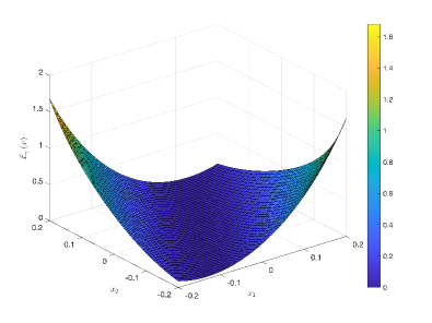
Figure 1: Past energy function $\mathcal{E}_{\gamma}^{-}$ for the model (42)–(43) in the original coordinates.

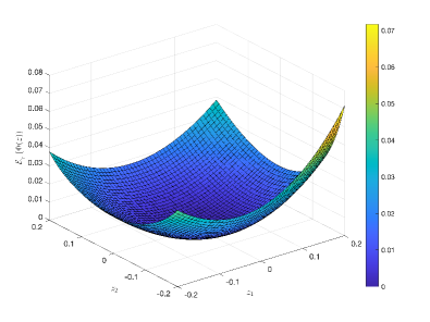
Figure 2: Past energy function $\mathcal{E}_{\gamma}^{-}$ for the model (42)–(43) using a linear state transformation, $\mathbf{x}=\mathbf{T}_{1}\mathbf{z}$.

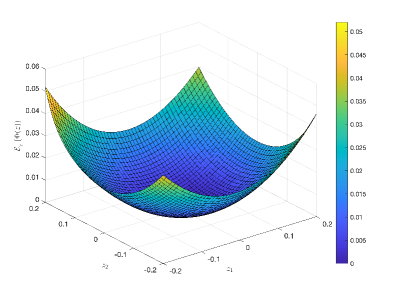
Figure 3: Past energy function $\mathcal{E}_{\gamma}^{-}$ for the model (42)–(43) using a quadratic state transformation, $\mathbf{x}=\mathbf{T}_{1}\mathbf{z}+\mathbf{T}_{2}(\mathbf{z}\otimes\mathbf{z})$.

Table 1: The effect of varying degree transformations on maximum error in the transformed past energy function $\mathcal{E}_{\gamma}^{-}$ over the domain $(-a,a)^{2}$.

degree	$a=0.2$	$a=0.05$	$a=0.01$
1	4.0566e-02	1.5498e-04	1.0886e-06
2	1.8411e-02	7.6587e-06	9.2309e-09
3	1.6217e-02	1.7734e-06	4.2417e-10
4	1.8339e-02	4.2031e-07	1.9737e-11
5	1.6364e-02	1.0820e-07	1.0743e-12
6	1.8547e-02	2.3594e-08	6.2827e-14
7	1.5997e-02	1.7912e-08	4.7472e-15
8	1.9368e-02	1.1080e-08	1.0545e-15

3.2 Input-output balancing transformation

The transformation in Section 3.1 brings the system into the input-normal/output-diagonal form, see Theorem 1. The next theorem suggests a transformation that brings the system into the widely-used input-output balanced form, where the singular values appear in both the controllability and observability energy functions.

Theorem 3.7.

[20, Thm. 9] Suppose that the Jacobian linearization of the nonlinear system is controllable, observable, and asymptotically stable. Then there is a neighborhood $\mathcal{W}$ of the origin and a smooth coordinate transformation $\mathbf{x}=\bar{\Phi}(\bar{\mathbf{z}})$ on $\mathcal{W}$ converting the controllability and observability energy functions into the form

$$\mathcal{E}_{c}(\bar{\Phi}(\bar{\mathbf{z}})) =\frac{1}{2}\sum_{i=1}^{n}\frac{\bar{z}_{i}^{2}}{{\sigma}_{i}(\bar{z}_{i})},$$ (44)

$$\mathcal{E}_{o}(\bar{\Phi}(\bar{\mathbf{z}})) =\frac{1}{2}\sum_{i=1}^{n}{\sigma}_{i}(\bar{z}_{i})\bar{z}_{i}^{2}.$$ (45)

Moreover, if $\mathcal{W}=\mathbb{R}^{n}$, then the Hankel norm of the nonlinear system is given by

$$\|\Sigma\|_{H}:=\sup_{\mathbf{u}\in L_{2}(\mathbb{R}^{+}),\mathbf{u}\neq\mathbf{0}}\frac{\|\mathcal{H}(\mathbf{u})\|}{\|\mathbf{u}\|}=\sup_{\bar{z}_{1}}{\sigma}_{1}(\bar{z}_{1}),$$ (46)

where $\mathcal{H}$ is the Hankel operator for the nonlinear system.

Such a variable transformation also exits under more technical assumptions for closed-loop system, see [46, Thm 5.13], where the past and future energy functions $\mathcal{E}_{\gamma}^{-}$ and $\mathcal{E}_{\gamma}^{+}$ are transformed into input-output form, and where the underlying system is potentially unstable. Note that since each singular value function in (44) is associated with a single state component $z_{i}$, they can be used to decide the truncation of the states, see Section 4. To obtain the transformation $\bar{\Phi}(\bar{\mathbf{z}})$, first consider the past energy function in input-normal form, i.e., $\mathcal{E}_{\gamma}^{-}(\Phi(\mathbf{z}))=\frac{1}{2}\sum_{i=1}^{n}z_{i}^{2}$ from (10). We now need to scale the individual states to obtain $\mathcal{E}_{\gamma}^{-}(\bar{\Phi}(\bar{\mathbf{z}}))=\frac{1}{2}\sum_{i=1}^{n}\frac{\bar{z}_{i}^{2}}{{\sigma}_{i}(\bar{z}_{i})}$. To do this, consider the nonlinear transformation

$$\bar{z}_{i}=z_{i}\sqrt{\xi_{i}(z_{i})}=\bar{\Phi}_{i}^{-1}(z_{i})\quad\Rightarrow\quad\bar{\Phi}_{i}(\bar{z}_{i})=z_{i}.$$ (47)

We insert this transformation into the energy function in (10) and obtain

$$\mathcal{E}_{\gamma}^{-}(\bar{\Phi}(\bar{\mathbf{z}})) =\frac{1}{2}\sum_{i=1}^{n}\frac{\bar{z}_{i}^{2}}{\xi_{i}(z_{i})}$$

$$=\frac{1}{2}\sum_{i=1}^{n}\frac{\bar{z}_{i}^{2}}{\xi_{i}(\bar{\Phi}_{i}(\bar{z}_{i}))}=\frac{1}{2}\sum_{i=1}^{n}\frac{\bar{z}_{i}^{2}}{\sigma_{i}(\bar{z}_{i})},$$ (48)

where the new input-output singular value functions are defined (see [20, Thm 11]) as

$$\sigma_{i}(\bar{z}_{i}):=\xi_{i}(\bar{\Phi}_{i}(\bar{z}_{i}))=\xi_{i}(z_{i}).$$ (49)

This implies that the singular value functions of the input-normal/output-diagonal and the input-output balancing transformations are identical. To clarify this point, let us recall the linear case. For an LTI system, let $\mathbf{Y}_{\infty}$ and $\mathbf{X}_{\infty}$ be the solutions to the the $\mathcal{H}_{\infty}$ AREs (17) and (18), respectively. Then, the input normal form would imply that $\mathbf{Y}_{\infty}=\mathbf{I}$ and $\mathbf{X}_{\infty}=\operatorname{diag}(\xi_{1}(0)^{2},\ldots,\xi_{n}(0)^{2})$. However, since the $\mathcal{H}_{\infty}$-characteristic values $\xi_{i}(0)$, which are the Hankel singular values in the limit $\gamma\rightarrow 1$ in (3)–(5), are invariant under state-space transformation, in the fully balanced coordinates (after proper scaling) one would have $\mathbf{Y}_{\infty}=\mathbf{X}_{\infty}=\operatorname{diag}(\xi_{1}(0),\ldots,\xi_{n}(0))$.

Next, we consider how the nonlinear state transformation (47) affects the future energy function of the input-normal/output-diagonal form, $\mathcal{E}_{\gamma}^{+}(\Phi(\mathbf{z}))=\frac{1}{2}\sum_{i=1}^{n}z_{i}^{2}\xi_{i}^{2}(z_{i})$. Applying the nonlinear transformation from (47), it follows that the future energy function is automatically transformed into the input-output balanced form as in Theorem 3.7:

$$\mathcal{E}_{\gamma}^{+}(\bar{\Phi}(\bar{\mathbf{z}})) =\frac{1}{2}\sum_{i=1}^{n}\bar{z}_{i}^{2}\xi_{i}(z_{i})=\frac{1}{2}\sum_{i=1}^{n}\bar{z}_{i}^{2}\xi_{i}(\bar{\Phi}(\bar{z}_{i}))$$

$$=\frac{1}{2}\sum_{i=1}^{n}\bar{z}_{i}^{2}\sigma_{i}(\bar{z}_{i}),$$ (50)

with the the singular value functions from (49).

Remark 3.8.

The connection to balanced truncation for LTI systems can be further appreciated by writing the energy functions in (44) in the form

$$\mathcal{E}_{\gamma}^{-}(\bar{\Phi}(\bar{\mathbf{z}})) =\frac{1}{2}\bar{\mathbf{z}}^{\top}\mathbf{\Sigma}(\bar{\mathbf{z}})^{-1}\bar{\mathbf{z}},$$ (51)

$$\quad\mathcal{E}_{\gamma}^{+}(\bar{\Phi}(\bar{\mathbf{z}})) =\frac{1}{2}\bar{\mathbf{z}}^{\top}\mathbf{\Sigma}(\bar{\mathbf{z}})\bar{\mathbf{z}}$$ (52)

where $\mathbf{\Sigma}(\bar{\mathbf{z}})={\rm{diag}}({\sigma}_{1}(\bar{z}_{1}),\ldots,{\sigma}_{n}(\bar{z}_{n}))$. The interpretation of this form is to consider the ‘Gramian’ in the balanced coordinates$,\mathbf{\Sigma}(\bar{\mathbf{z}})$, as state dependent, as opposed to it being constant in the LTI case.

3.3 Balanced high-dimensional model

The nonlinear transformation from Theorem 3.7 and (47) that brings the dynamical system (1)–(2) into the input-output balanced coordinate system can be summarized as

$$\begin{cases}\mathbf{x}&=\bar{\Phi}(\bar{\mathbf{z}})=\mathbf{T}_{1}\mathbf{z}+\mathbf{T}_{2}\mathbf{z}^{\leavevmode\hbox to6.15pt{\vbox to6.15pt{\text{[drawing]}}}}+\cdots+\mathbf{T}_{k}\mathbf{z}^{\leavevmode\hbox to6.44pt{\vbox to6.44pt{\text{[drawing]}}}}\\ z_{i}&=\bar{z}_{i}/\sqrt{\sigma_{i}(\bar{z}_{i})}.\end{cases}$$ (53)

Note that the transformation matrices $\mathbf{T}_{i}$ did not change, as the input-normal/output-diagonal form is already diagonalized, but the scaling has. In other words, using (49) each new state is now scaled by $\sqrt{\xi_{i}(z_{i})}$ to get the fully balanced form from Theorem 3.7. In the LTI case, $\mathbf{x}=\mathbf{T}_{1}\mathbf{z}$ from (12) yields the input-normal/output-diagonal and by an additional scaling of the state, $\bar{z}_{i}/\sqrt{\xi_{i}(0)}=z_{i}$ we obtain the transformation $\mathbf{x}=\mathbf{T}_{1}{\mathbf{z}}=\mathbf{T}_{1}\mathbf{\Sigma}^{-1/2}\bar{\mathbf{z}}$ which is the input-output balanced form in (53).

The dynamical system when transformed with the input-output balancing transformation $\mathbf{x}=\bar{\Phi}(\bar{\mathbf{z}})$ is

$$\bar{\mathbf{J}}(\bar{\mathbf{z}})\dot{\bar{\mathbf{z}}}=\mathbf{f}(\bar{\Phi}(\bar{\mathbf{z}}))+\mathbf{g}(\bar{\Phi}(\bar{\mathbf{z}}))\mathbf{u},$$ (54)

where the Jacobian $\bar{\mathbf{J}}(\bar{\mathbf{z}})\in\mathbb{R}^{n\times n}$ of the state-space transformation is given by

$$\bar{\mathbf{J}}(\bar{\mathbf{z}}):= \frac{\text{d}{\bar{\Phi}(\bar{\mathbf{z}})}}{\text{d}\bar{\mathbf{z}}}$$ (55)

$$= \mathbf{T}_{1}+2\mathbf{T}_{2}(\bar{\mathbf{z}}\otimes\mathbf{I})+3\mathbf{T}_{3}(\bar{\mathbf{z}}\otimes\bar{\mathbf{z}}\otimes\mathbf{I})+\ldots,$$

where we used the fact that since we compute $\mathbf{T}_{k}$ with symmetric coefficients, it follows that, e.g., $\mathbf{T}_{2}(\bar{\mathbf{z}}\otimes\mathbf{I})=\mathbf{T}_{2}(\mathbf{I}\otimes\bar{\mathbf{z}})$. See Definition 1 for more details on symmetric coefficients. The Jacobian can be computed explicitly without numerical approximation, as it is the derivative of a polynomial transformation. Remarkably, the Jacobian $\frac{\text{d}{\Phi(\mathbf{z}})}{\text{d}\mathbf{z}}$ of the input-normal/output-diagonal transformation (12) and the Jacobian $\frac{\text{d}{\bar{\Phi}(\bar{\mathbf{z}})}}{\text{d}\bar{\mathbf{z}}}$ of the input-output balancing transformation (53) have the same coefficient matrices $\mathbf{T}_{i}$, which significantly simplifies the ROM simulation. In the next section we revisit the standard balancing transformation that typically results in conditioning problems. We then introduce a novel approximation to simultaneously balance-and-reduce nonlinear systems in a well-conditioned and computationally efficient way.

4 Balanced truncation model reduction via nonlinear transformations

In this section, we reduce the dimensionality of the fully balanced model (54). To determine the reduced dimension $r$ of the ROM, we look for a significant gap in the $\mathcal{H}_{\infty}$ singular value functions, i.e., we look for the reduced dimension $r$ such that

$$\max_{\bar{z}_{r}}\sigma_{r}(\bar{z}_{r})\gg\max_{\bar{z}_{r+1}}\sigma_{r+1}(\bar{z}_{r+1})$$ (56)

(at a minimum we require that ‘$>$’ holds) in a neighborhood of the origin. This indicates that the state components $\bar{z}_{1},\bar{z}_{2},\ldots,\bar{z}_{r}$ are more important in terms of the past and future energy functions $\mathcal{E}_{\gamma}^{-}$ and $\mathcal{E}_{\gamma}^{+}$ than the states $\bar{z}_{r+1},\bar{z}_{r+2},\ldots,\bar{z}_{n}$. We therefore set $\bar{z}_{r+1}=\bar{z}_{r+2}=\ldots=\bar{z}_{n}=0$ in the balanced coordinates and define the reduced state vector as

$$\bar{\mathbf{z}}_{r}=\mathbf{\Psi}_{r}^{\top}\ \bar{\mathbf{z}}=[\bar{z}_{1},\bar{z}_{2},\ldots\bar{z}_{r}]^{\top},\quad\mathbf{\Psi}_{r}=\begin{bmatrix}\mathbf{I}_{r}&\mathbf{0}\end{bmatrix}^{\top}\in\mathbb{R}^{n\times r}.$$ (57)

The next Section 4.1 presents the originally-proposed balanced ROM from [45, 46]. Section 4.2 proposes a novel and numerically more efficient and better conditioned approximate strategy to compute the nonlinear ROMs corresponding to this truncation strategy. Section 4.3 suggests a different perspective of the nonlinear ROM, namely the approximation on a nonlinear balanced manifold.

4.1 Balance-then-reduce approach

The balance-then-reduce strategy suggested in [45, 46] first computes the full balancing transformation, and then truncates the resulting fully balanced system. Applying this to equation (54) yields

$$\dot{\bar{\mathbf{z}}}_{r}= \underbrace{\mathbf{\Psi}_{r}^{\top}[\bar{\mathbf{J}}([\bar{\mathbf{z}}_{r},\mathbf{0}])]^{-1}\mathbf{f}(\bar{\Phi}([\bar{\mathbf{z}}_{r},\mathbf{0}]))}_{=:\mathbf{f}_{r}(\bar{\mathbf{z}}_{r})}$$

$$+\underbrace{\mathbf{\Psi}_{r}^{\top}[\bar{\mathbf{J}}([\bar{\mathbf{z}}_{r},\mathbf{0}])]^{-1}\mathbf{g}(\bar{\Phi}([\bar{\mathbf{z}}_{r},\mathbf{0}]))}_{=:\mathbf{g}_{r}(\bar{\mathbf{z}}_{r})}\mathbf{u},$$ (58)

$$\mathbf{y}_{r}= \underbrace{\mathbf{h}(\bar{\Phi}([\bar{\mathbf{z}}_{r},\mathbf{0}]))}_{=:\mathbf{h}_{r}(\bar{\mathbf{z}}_{r})}.$$ (59)

The high-dimensional state is reconstructed as $\mathbf{x}\approx\bar{\Phi}([\bar{\mathbf{z}}_{r},\mathbf{0}])$. A goal of balanced truncation is to obtain ROMs that are balanced in the reduced coordinates and that retain properties of the FOM, such as stability. The following theorems show that obtaining such results depends on which energy functions are used for balancing. First, we consider the case of balancing the open-loop energy functions from (6).

Theorem 4.9.

[20, Thm. 10] Consider the nonlinear dynamical system (1)–(2). Suppose that

1. the open-loop controllability and observability energy functions $\mathcal{E}_{c}$ and $\mathcal{E}_{o}$ exist,

2. the matrices $\left[\frac{\partial^{2}\mathcal{E}_{c}(\mathbf{x})}{\partial x_{i}\partial x_{j}}(\mathbf{0})\right]_{i,j=1,\ldots n}$ and $\left[\frac{\partial^{2}\mathcal{E}_{o}(\mathbf{x})}{\partial x_{i}\partial x_{j}}(\mathbf{0})\right]_{i,j=1,\ldots n}$ are positive definite,

3. the eigenvalues of $\left[\frac{\partial^{2}\mathcal{E}_{c}(\mathbf{x})}{\partial x_{i}\partial x_{j}}(\mathbf{0})\right]^{-1}\left[\frac{\partial^{2}\mathcal{E}_{o}(\mathbf{x})}{\partial x_{i}\partial x_{j}}(\mathbf{0})\right]$ are distinct.

Then, with the input-output balancing transformation $\bar{\Phi}(\bar{\mathbf{z}})$, the controllability function $\mathcal{E}_{c,r}$ and observability energy function $\mathcal{E}_{o,r}$ of the balanced ROM (58)–(59) satisfy

$$\mathcal{E}_{c,r}(\bar{\mathbf{z}}_{r})=\mathcal{E}_{c}([\bar{\mathbf{z}}_{r},\mathbf{0}]),\quad\mathcal{E}_{o,r}(\bar{\mathbf{z}}_{r})=\mathcal{E}_{o}([\bar{\mathbf{z}}_{r},\mathbf{0}]).$$ (60)

Moreover, the singular value functions $\sigma_{i,r}(\bar{z}_{i})$ of the ROM similarly satisfy

$$\sigma_{i,r}(\bar{z}_{i})=\sigma_{i}(\bar{z}_{i}),$$ (61)

and the energy functions of the ROM are balanced in the sense of Theorem 3.7.

Remark 4.10.

From Theorem 4.9 we see that under suitable assumptions, the open-loop energy functions are preserved at the ROM level. This implies that the ROM inherits the local asymptotic stability of the FOM [45, Thm 5.3]. In some special cases global asymptotic stability can be guaranteed, see [45, Thm 5.4]. pp

The next theorem addresses the case when balancing is performed with the closed-loop $\mathcal{H}_{\infty}$ (past and future) energy functions (3)–(4). In this scenario, an extra condition is needed so that the ROMs remain balanced in the reduced coordinates as well.

Theorem 4.11.

[46, Thm 6.1.] Let $\check{\mathbf{z}}=[\bar{z}_{r+1},\ldots,\bar{z}_{n}]$ be the vector of state components that are truncated from the FOM. Correspondingly, let the input-output balanced system (54) be partitioned as $[\dot{\bar{\mathbf{z}}}_{r};\dot{\check{\mathbf{z}}}]^{\top}=[\mathbf{f}_{1}(\bar{\mathbf{z}});\mathbf{f}_{2}(\bar{\mathbf{z}})]^{\top}+[\mathbf{g}_{1}(\bar{\mathbf{z}});\mathbf{g}_{2}(\bar{\mathbf{z}})]^{\top}\mathbf{u}$. Suppose that the closed-loop energy functions $\mathcal{E}_{\gamma}^{-}$ and $\mathcal{E}_{\gamma}^{+}$ from  (3)–(4) exist. With the input-output balancing transformation $\bar{\Phi}(\bar{\mathbf{z}})$, the past energy function of the balanced ROM (58)–(59) satisfies

$$\mathcal{E}_{\gamma}^{-}(\bar{\mathbf{z}}_{r})=\mathcal{E}_{\gamma}^{-}([\bar{\mathbf{z}}_{r},\mathbf{0}]).$$ (62)

Assume further that

$$\frac{\partial\mathcal{E}_{\gamma}^{+}}{\partial\check{\mathbf{z}}}(\bar{\mathbf{z}}_{r},\mathbf{0})\mathbf{f}_{2}(\bar{\mathbf{z}}_{r},\mathbf{0})=0,\quad\frac{\partial\mathcal{E}_{\gamma}^{+}}{\partial\check{\mathbf{z}}}(\bar{\mathbf{z}}_{r},\mathbf{0})\mathbf{g}_{2}(\bar{\mathbf{z}}_{r},\mathbf{0})=0$$ (63)

holds; then the future energy function satisfies

$$\qquad\mathcal{E}_{\gamma}^{+}(\bar{\mathbf{z}}_{r})=\mathcal{E}_{\gamma}^{+}([\bar{\mathbf{z}}_{r},\mathbf{0}]).$$ (64)

Since the original system is not assumed stable in the $\mathcal{H}_{\infty}$ framework, an interesting property to study is whether the reduce-then-design strategy for the $\mathcal{H}_{\infty}$ suboptimal control is guaranteed to produce a suboptimal control for the $\mathcal{H}_{\infty}$-balanced ROM. For conditions when that holds true, we refer to [46, Thm 6.3].

The evaluation of the polynomials terms on the right-hand side of the ROM (58) can be simplified for the special case $\mathbf{f}(\mathbf{z})=\mathbf{A}\mathbf{z}+\mathbf{N}(\mathbf{z}\otimes\mathbf{z})$, which yields

$$\mathbf{f}(\bar{\Phi}([\bar{\mathbf{z}}_{r},\mathbf{0}]))=\sum_{i=1}^{k}[\mathbf{A}\mathbf{T}_{i}\mathbf{I}_{n\times r}^{\leavevmode\hbox to5.61pt{\vbox to5.61pt{\text{[drawing]}}}}]\bar{\mathbf{z}}_{r}^{\leavevmode\hbox to5.61pt{\vbox to5.61pt{\text{[drawing]}}}}$$

$$\qquad+\mathbf{N}\left(\sum_{i=1}^{k}[\mathbf{T}_{i}\mathbf{I}_{n\times r}^{\leavevmode\hbox to5.61pt{\vbox to5.61pt{\text{[drawing]}}}}]\bar{\mathbf{z}}_{r}^{\leavevmode\hbox to5.61pt{\vbox to5.61pt{\text{[drawing]}}}}\otimes\sum_{i=1}^{k}[\mathbf{T}_{i}\mathbf{I}_{n\times r}^{\leavevmode\hbox to5.61pt{\vbox to5.61pt{\text{[drawing]}}}}]\bar{\mathbf{z}}_{r}^{\leavevmode\hbox to5.61pt{\vbox to5.61pt{\text{[drawing]}}}}\right).$$ (65)

Nevertheless, simulating the ROM (58) is computationally expensive and will likely result in inverting an ill-conditioned matrix, which is in analogy to the linear case. In the next section, we propose a better conditioned and computationally more efficient implementation of the nonlinear ROM.

4.2 Simultaneous balancing and reduction

The computation of $\mathbf{\Psi}_{r}^{\top}[\bar{\mathbf{J}}([\bar{\mathbf{z}}_{r},\mathbf{0}])]^{-1}$ in the balanced ROM (58)–(59) requires inverting the full Jacobian followed by truncation. This has a computational and a numerical disadvantage. First, this strategy requires a high number of floating point operations to form the full $\mathbf{T}_{j}\in\mathbb{R}^{n\times n^{j}},\ j=2,\ldots,k$ as in Theorem 2. Second, computing $\mathbf{T}_{1}$ requires inversions that are often ill-conditioned for large-scale systems (the main focus of this work) since it requires inverting all the $\mathcal{H}_{\infty}$-characteristic values, including the smallest ones. In the linear case, the balance-then-reduce strategy is well known to be ill-conditioned due to small Hankel singular values, see, e.g., [2, Sec. 7.3] and a remedy is to perform simultaneous model reduction and truncation.

We suggest a new computational framework for the nonlinear case following these ideas from the linear case. Our goal is to compute the truncated versions of the linear transformations and higher-degree tensors $\{\mathbf{T}_{i}\}_{i=1}^{k}$ from Theorem 2 directly without computing the full-order quantities. We begin with deriving the form of the nonlinear ROM for the FOM (1)–(2) when a general polynomial state transformation and simultaneous reduction is applied. In other words, we are approximating the FOM (1)–(2) on a nonlinear (here: balanced) manifold such that $\mathbf{x}\approx\Phi_{r}(\bar{\mathbf{z}}_{r})$, where the mapping $\Phi_{r}$ defines a manifold. The following result applies to any polynomial state transformation.

Proposition 4.12.

Consider the nonlinear system (1)–(2). Let $\mathbf{T}_{k,r}\in\mathbb{R}^{n\times r^{k}}$ be (truncated) transformation matrices with symmetric coefficients and $\bar{\mathbf{z}}_{r}\in\mathbb{R}^{r}$ denote the reduced state. Define the embedding $\Phi_{r}:\mathbb{R}^{r}\mapsto\mathbb{R}^{n}$ via

$$\mathbf{x}\approx\Phi_{r}(\bar{\mathbf{z}}_{r}):=\mathbf{T}_{1,r}\bar{\mathbf{z}}_{r}+\mathbf{T}_{2,r}\bar{\mathbf{z}}_{r}^{\leavevmode\hbox to6.15pt{\vbox to6.15pt{\text{[drawing]}}}}+\cdots+\mathbf{T}_{k,r}\bar{\mathbf{z}}_{r}^{\leavevmode\hbox to6.44pt{\vbox to6.44pt{\text{[drawing]}}}},$$ (66)

for which the reduced Jacobian can be computed explicitly via

$$\mathbf{J}_{r}(\bar{\mathbf{z}}_{r}):= \frac{{\rm{d}}\Phi_{r}(\bar{\mathbf{z}}_{r})}{{\rm{d}}\bar{\mathbf{z}}_{r}}$$

$$= \mathbf{T}_{1,r}+2\mathbf{T}_{2,r}(\bar{\mathbf{z}}_{r}\otimes\mathbf{I})$$

$$+3\mathbf{T}_{3,r}(\bar{\mathbf{z}}_{r}\otimes\bar{\mathbf{z}}_{r}\otimes\mathbf{I})+\cdots\in\mathbb{R}^{n\times r}.$$ (67)

Thus, the nonlinear ROM for $\bar{\mathbf{z}}_{r}\in\mathbb{R}^{r}$ is

$$\dot{\bar{\mathbf{z}}}_{r} =\underbrace{\mathbf{J}_{r}(\bar{\mathbf{z}}_{r})^{\dagger}\mathbf{f}(\Phi_{r}(\bar{\mathbf{z}}_{r}))}_{=:\mathbf{f}_{r}(\bar{\mathbf{z}}_{r})}+\underbrace{\mathbf{J}_{r}(\bar{\mathbf{z}}_{r})^{\dagger}\mathbf{g}(\Phi_{r}(\bar{\mathbf{z}}_{r}))}_{=:\mathbf{g}_{r}(\bar{\mathbf{z}}_{r})}\mathbf{u}$$ (68)

$$\mathbf{y}_{r} =\underbrace{\mathbf{h}(\Phi_{r}(\bar{\mathbf{z}}_{r}))}_{=:\mathbf{h}_{r}(\bar{\mathbf{z}}_{r})}.$$ (69)

where $[\cdot]^{\dagger}$ denotes the Moore-Penrose pseudoinverse.

Proof 4.13.

Given $\Phi_{r}(\bar{\mathbf{z}}_{r})$ in (66) and using the symmetry arguments as in (55) (which result from our symmetrized computation of the $\mathbf{T}_{i,r}$), we can directly verify the polynomial form of the Jacobian following (55) with $\bar{\mathbf{z}}_{r}$ instead of $\bar{\mathbf{z}}$, thus obtaining (4.12). With this reduced Jacobian defined, the model (54) becomes

$$\mathbf{J}_{r}(\bar{\mathbf{z}}_{r})\dot{\mathbf{z}}_{r}=\mathbf{f}(\Phi_{r}(\bar{\mathbf{z}}_{r}))+\mathbf{g}(\Phi_{r}(\bar{\mathbf{z}}_{r}))\mathbf{u}\in\mathbb{R}^{n}.$$ (70)

We left-multiply the last equation with the pseudo-inverse of the Jacobian to get the ROM (68)–(69).

The version of the ROM formulated in Proposition 4.12 resolves the ill-conditioning issue since it no longer requires inverting the full Jacobian. Now, what is needed is a strategy that could compute the coefficient matrices, $\mathbf{T}_{i,r}\in\mathbb{R}^{n\times r^{i}}$ of the nonlinear embedding $\Phi_{r}$ without needing to construct full coefficient matrices, $\mathbf{T}_{i}\in\mathbb{R}^{n\times n^{i}}$. Following Theorem 2 and Algorithm 1 and motivated by the linear balanced truncation framework, in the next result we propose a new strategy to compute the matrices $\mathbf{T}_{i,r}$ of the nonlinear balancing transformation (66). Before stating this result, we point out that the ROM computation in (68) still requires evaluating the full $\mathbf{f}(\cdot)$ and $\mathbf{g}(\cdot)$ as nonlinear functions acting on vectors of dimension $n$. We revisit and resolve this issue—known as the lifting bottleneck—in Remark 4.17.

Proposition 4.14.

(Truncated (approximate) balanced transformation) Let $\mathbf{v}_{i},\mathbf{w}_{i}$ be the vectors of polynomial coefficients for the energy functions from (7), (9). Let $\mathbf{R},\mathbf{L}$ be their Cholesky factors, i.e., $\mathbf{V}_{2}=\mathbf{R}\mathbf{R}^{\top}$ and $\mathbf{W}_{2}=\mathbf{L}\mathbf{L}^{\top}$. Let $\mathbf{L}^{\top}\mathbf{R}^{-\top}=\mathcal{U}\mathbf{\Xi}\mathcal{V}^{\top}$ be the singular value decomposition and define

$$\mathcal{U}_{r}=\mathcal{U}(:,1:r),\leavevmode\nobreak\ \leavevmode\nobreak\ \mathbf{\Xi}_{r}=\mathbf{\Xi}(1:r,1:r),\leavevmode\nobreak\ \leavevmode\nobreak\ \mathcal{V}_{r}=\mathcal{V}(:,1:r).$$

Then, the coefficient matrices of the nonlinear embedding $\Phi_{r}:\mathbb{R}^{r}\mapsto\mathbb{R}^{n}$ in (66) are

$$\mathbf{T}_{1,r} =\mathbf{R}^{-\top}\mathcal{V}_{r}\in\mathbb{R}^{n\times r},$$ (71)

$$\mathbf{T}_{1,r}^{\dagger} =\mathbf{\Xi}_{r}^{-1}\mathcal{U}_{r}^{\top}\mathbf{L}^{\top}\in\mathbb{R}^{r\times n},\ \text{(left inverse)}$$ (72)

$$\mathbf{T}_{2,r} =-\frac{1}{2}\mathbf{T}_{1,r}\ {\text{unvec}}\left([\mathbf{T}_{1,r}^{\leavevmode\hbox to6.15pt{\vbox to6.15pt{\text{[drawing]}}}}]^{\top}\mathbf{v}_{3}\right)^{\top}\in\mathbb{R}^{n\times r^{2}},$$ (73)

and more generally, for $2\leq k$,

$$\mathbf{T}_{k,r} =-\frac{1}{2}\mathbf{T}_{1,r}{\text{unvec}}(\mathbf{M}_{k,r})^{\top}\in\mathbb{R}^{n\times r^{k}},\leavevmode\nobreak\ \mbox{where}$$ (74a)

$$\mathbf{M}_{k,r} =\sum_{\begin{subarray}{c}i,j>1\\ i+j=k+1\end{subarray}}{\text{vec}}\left(\mathbf{T}_{j,r}^{\top}\mathbf{V}_{2}\mathbf{T}_{i,r}\right)+\sum_{i=3}^{k+1}\mathcal{T}_{i,k+1}^{\top}\mathbf{v}_{i}.$$ (74b)

We highlight that due to the way we compute $\mathbf{T}_{i,r}$ above, the embedding, and hence Jacobian, is better conditioned and faster to evaluate than in the balance-then-reduce strategy in Section 4.1. The next theorem shows that the linear part of the transformation diagonalizes the product of the Gramians, as in the linear case.

Proposition 4.15.

The approximate balancing transformation (66) with $\mathbf{T}_{i,r}$ from Proposition 4.14 satisfies

$$\mathbf{\Xi}_{r}^{2}={\text{diag}}(\xi_{1}^{2}(0),\ldots,\xi_{r}^{2}(0))=\mathbf{T}_{1,r}^{\dagger}\mathbf{V}_{2}^{-1}\mathbf{W}_{2}\mathbf{T}_{1,r}.$$ (75)

Proof 4.16.

Given the definitions of Proposition 4.14 we directly compute

$$\mathbf{T}_{1,r}^{\dagger}\mathbf{V}_{2}^{-1}\mathbf{W}_{2}\mathbf{T}_{1,r}$$

$$=\mathbf{\Xi}_{r}^{-1}\mathcal{U}_{r}^{\top}\mathbf{L}^{\top}\mathbf{R}^{-\top}\mathbf{R}^{-1}\mathbf{L}\mathbf{L}^{\top}\mathbf{R}^{-\top}\mathcal{V}_{r}$$

$$=\mathbf{\Xi}_{r}^{-1}\mathcal{U}_{r}^{\top}\mathcal{U}_{r}\mathbf{\Xi}_{r}\mathcal{V}_{r}^{\top}\mathcal{V}_{r}\mathbf{\Xi}_{r}\mathcal{U}_{r}^{\top}\mathcal{U}_{r}\mathbf{\Xi}_{r}\mathcal{V}_{r}^{\top}\mathcal{V}_{r}$$

$$=\mathbf{\Xi}_{r}^{-1}\mathbf{\Xi}_{r}^{3}=\mathbf{\Xi}_{r}^{2}$$

With a numerically well-conditioned ROM (68)–(69) and a computationally efficient way to compute the nonlinear balanced manifold, see Proposition 4.14, we summarize the steps to arrive at a simultaneously balanced-and-reduced ROM in Algorithm 3.

Algorithm 3 Computation of nonlinear input-output $\mathcal{H}_{\infty}$-balanced ROM.

1:Constant $\gamma>\gamma_{0}\geq 0$, $\gamma\neq 1$; polynomial degrees $d>k>\ell$; reduced model order $r$

2:Input-output nonlinear $\mathcal{H}_{\infty}$-balanced ROM (68)–(69).

3:Obtain a polynomial representation (or approximation) of the past and future energy functions $\mathcal{E}_{\gamma}^{-}(\mathbf{x})$ and $\mathcal{E}_{\gamma}^{+}(\mathbf{x})$, i.e., coefficients $\left\{\mathbf{v}_{i}\right\}_{i=2}^{d}$ and $\left\{\mathbf{w}_{i}\right\}_{i=2}^{d}$ in (7), (9) (e.g., through Part 1 of this paper[30])

4:Compute the truncated polynomial coefficient matrices $\left\{\mathbf{T}_{i,r}\right\}_{i=1}^{k}$ for $\mathbf{x}\approx\Phi_{r}(\bar{\mathbf{z}}_{r})$ from (66) following Proposition 4.14.

5:Symmetrize the coefficients $\left\{\mathbf{T}_{i,r}\right\}_{i=1}^{r}$ (see Remark 2)

6:Assemble the nonlinear ROM functions $\mathbf{f}_{r}(\bar{\mathbf{z}}_{r}),\mathbf{g}_{r}(\bar{\mathbf{z}}_{r}),\mathbf{h}_{r}(\bar{\mathbf{z}}_{r})$ as in  (68)–(69) with the explicit Jacobian in (4.12).

Algorithm 3 requires a choice of ROM dimension $r$. This can be done by plotting all state-dependent singular value functions from (13), whose coefficients are obtained via Algorithm 2, and deciding on an ordering of the functions in magnitude. However, this procedure increases the (offline) cost of the algorithm, as all $\mathbf{c}_{i}$ and $\mathbf{T}_{i}$, for $i=1,2,\ldots,n$ are required. To reduce the offline cost, it may be enough in some cases to only consider the constant terms $\xi_{i}(0)$ in the singular value functions to make a truncation decision based on their decay, as is done in balanced truncation for LTI systems.

Remark 4.17.

Algorithm 3 helps to resolve the computational complexity and numerical ill-conditioning issues of the balance-then-reduce strategy using the simultaneous (approximate) balancing-and-reduce strategy. However, as stated earlier, we point out that the ROM computation in (68)-(69) still requires evaluating the full $\mathbf{f}(\cdot)$ and $\mathbf{g}(\cdot)$ as nonlinear functions acting on vectors of dimension $n$. This is a common issue in nonlinear model reduction not specific to nonlinear balanced truncation. If the inputs and outputs are linear, then $\mathbf{g}_{r}(\bar{\mathbf{z}}_{r})=\mathbf{J}_{r}(\bar{\mathbf{z}}_{r})^{\dagger}\mathbf{B}$ and $\mathbf{h}_{r}(\bar{\mathbf{z}}_{r})=\mathbf{C}\Phi_{r}(\bar{\mathbf{z}}_{r})$ where all products of $\mathbf{C}$ and $\mathbf{T}_{k,r}$ can be precomputed. However, still the ROM in (68) requires evaluating the full nonlinearity. This could be circumvented by a hyper-reduction procedure, e.g., DEIM [13] and its variants [16, 17]. Only when the, inputs, outputs and dynamics are linear, then $\Phi(\bar{\mathbf{z}}_{r})=\mathbf{T}_{1,r}\bar{\mathbf{z}}_{r}$ and $\mathbf{J}_{r}(\bar{\mathbf{z}}_{r})=\mathbf{T}_{1,r}^{\dagger}$, so the linear ROM becomes

$$\dot{\bar{\mathbf{z}}}_{r}=\mathbf{T}_{1,r}^{\dagger}\mathbf{A}\mathbf{T}_{1,r}\bar{\mathbf{z}}_{r}+\mathbf{T}_{1,r}^{\dagger}\mathbf{B}\mathbf{u},\quad\mathbf{y}_{r}=\mathbf{C}\mathbf{T}_{1,r}\bar{\mathbf{z}}_{r},$$ (76)

where everything can be precomputed and the ROM can be simulated without any reference to the full dimension $n$.

4.3 Nonlinear balanced manifold ROMs

The described nonlinear balanced truncation approach performs model reduction on an $r$-dimensional polynomially-nonlinear manifold with specific structure. Nonlinear balanced truncation first performs a nonlinear balancing transformation $\mathbf{x}=\bar{\Phi}(\mathbf{z})$, which is followed by truncation. Thus, $\mathbf{x}\approx\Phi_{r}(\bar{\mathbf{z}}_{r}):=\mathbf{T}_{1,r}\bar{\mathbf{z}}_{r}+\mathbf{T}_{2,r}\bar{\mathbf{z}}_{r}^{\leavevmode\hbox to6.15pt{\vbox to6.15pt{\text{[drawing]}}}}+\cdots+\mathbf{T}_{k,r}\bar{\mathbf{z}}_{r}^{\leavevmode\hbox to6.44pt{\vbox to6.44pt{\text{[drawing]}}}}$ as in (66), which defines the nonlinear balancing manifold

$$\mathcal{M}:=\left\{\Phi_{r}(\bar{\mathbf{z}}_{r})\ :\ \bar{\mathbf{z}}_{r}\in\mathbb{R}^{r}\right\}\subseteq\mathbb{R}^{n}.$$ (77)

Figure 4 illustrates that the system evolves on this balanced nonlinear manifold (the $\bar{z}_{i}$-coordinates) of the original state space (the $x_{i}$-coordinates) such that the past and future energy (or controllability/observability energy) of a reduced state can be assessed via the well-known balanced form as outlined in Theorem 3.7. This fact then allows for truncation of individual states, as each state has associated energies. In the $\mathcal{H}_{\infty}$-balancing case, the retained ROM states are easy to filter and easy control. In the open-loop case, the retained states are easy to reach and easy to observe.

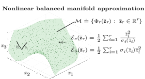
Figure 4: The input-output balanced ROM evolves on a nonlinear manifold, $\mathcal{M}$, such that the controllability/observability (or past/future) energy of a state can be measured in the well-known form that involves the singular value functions $\sigma_{i}(\bar{z}_{i})$.

Nonlinear manifold ROMs have become popular recently, as they address the challenges that linear subspace ROMs can face due to slow decay of the Kolmogorov $n$-width, see the survey article [42]. For instance, the authors in [34, 19] use a fully nonlinear autoencoder approach to define the nonlinear manifold ROM $\mathbf{x}\approx\psi(\bar{\mathbf{z}}_{r})$, while the work in [27, 22, 4] uses quadratic manifolds of the kind $\mathbf{x}\approx\mathbf{V}\bar{\mathbf{z}}_{r}+\bar{\mathbf{V}}(\bar{\mathbf{z}}_{r}\otimes\bar{\mathbf{z}}_{r})$. While these nonlinear manifold approaches improve the state-approximation error, they do not take into account the system-theoretic (observability/controllability) energies in the reduction, in turn neglecting the full dynamics of the input-to-output map.

5 Numerical Results: Burgers Equation

We present a proof-of-concept example that tests the effectiveness of the algorithms presented in Sections 3 and 4. The finite-dimensional model is generated from finite element discretizations of a PDE. The PDE of Burgers type is chosen for its quadratic nonlinear terms. This test problem has a long history in the study of control for distributed parameter systems, e.g. [50], including the development of effective computational methods, e.g. [12], and reduced-order models, e.g. [32]. Consider the controlled Burgers equation

$$\omega_{t}(\xi,t) =\epsilon\omega_{\xi\xi}(\xi,t)-\frac{1}{2}\left(\omega^{2}(\xi,t)\right)_{\xi}+\sum_{j=1}^{m}b_{j}^{m}(\xi)u_{j}(t),$$ (78)

$$y_{i}(t) =\int_{\chi_{[(i-1)/p,i/p]}}\omega(\xi,t)\text{d}\xi,\qquad i=1,\ldots,p,$$ (79)

with zero Dirichlet boundary conditions. Control inputs are described using the characteristic function $\chi$ as $b_{j}^{m}(\xi)=\chi_{[(j-1)/m,j/m]}(\xi)$ and the outputs are spatial averages of the solution over $p$ equally-spaced subdomains. We discretize the state equation with $n+1$ linear finite elements leading to an $n$-dimensional state vector. The discretized system has the form

$$\widetilde{\bf E}\dot{\boldsymbol{\omega}} =\widetilde{\bf A}{\boldsymbol{\omega}}+\widetilde{\bf N}_{2}\left({\boldsymbol{\omega}}\otimes{\boldsymbol{\omega}}\right)+\widetilde{\bf B}{\bf u}$$ (80)

$${\bf y} =\widetilde{\bf C}{\boldsymbol{\omega}},$$ (81)

where ${\boldsymbol{\omega}}(t)$ are the coefficients of the finite element approximation to $\omega(x,t)$. To place this in the form (1)–(2) where the mass matrix is the identity, we introduce the change of variables ${\bf x}=\widetilde{\bf E}^{1/2}{\boldsymbol{\omega}}$ where $\widetilde{\bf E}^{1/2}$ is a matrix square root of the finite element mass matrix. Then defining $\mathbf{A}=\widetilde{\bf E}^{-1/2}\widetilde{\mathbf{A}}\widetilde{\bf E}^{-1/2}$, $\mathbf{B}=\widetilde{\bf E}^{-1/2}\widetilde{\bf B}$, ${\bf C}=\widetilde{\bf C}\widetilde{\bf E}^{-1/2}$, ${\bf N}_{2}=\widetilde{\bf N}_{2}(\widetilde{\bf E}^{-1/2}\otimes\widetilde{\bf E}^{-1/2})$ leads to a system in the required form.

5.1 Singular value functions

In the first experiment, we use the values $\epsilon=0.05$, $n=16$, $m=4$, $p=4$, and $\gamma=3$, and we compute the quartic approximations to the past and future energy functions as described in Part 1 of this paper, [30], to find the coefficients in (7) and (9). Using these coefficients, we compute the cubic transformation tensors $\mathbf{T}_{1},\mathbf{T}_{2},\mathbf{T}_{3}$ using Algorithm 1. Finally, we compute quadratic approximations to the singular value functions as in Algorithm 2. The first eight of these are plotted in Figure 5. For this problem, we observe that the first four singular value functions are significantly larger in magnitude than the remainder. Moreover, the ranks of the singular value functions change across the variable range. We observe interesting behavior in the fifth singular value function, with a quadratic approximation that rapidly goes negative in a small region around zero. Although not plotted here for space, the cases with $p=1$ and $p=2$ outputs are different. In the $p=1$ case, the singular value functions do not cross in the same parameter interval; there is an order of magnitude separation of $\xi_{1}$, $\xi_{2}$, and $\xi_{3}$; there are nearly two orders of magnitude between $\xi_{5}$ and $\xi_{6}$. For the case $p=2$, there is a strong separation of the singular value functions near 0, but $\xi_{1}$ and $\xi_{2}$ do cross at about $|z|\approx 0.1$. We investigate the quality of ROMs with growing dimension in the next section and correlate the results with the qualitative behavior of the singular value functions.

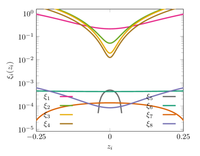
Figure 5: Quadratic approximations to the first eight singular value functions for the Burgers example.

5.2 Output behavior

We simulate the outputs for the system described above. We present results for different ROM-dimensions $r$ and different degree $k$ nonlinear transformations. We simulate the ROMs from $t=0$ to $t=10$ and report the relative error for each output, $e_{i}$, defined using

$$e_{i}=\frac{\left(\int_{0}^{10}\left|y_{i}(t)-y_{i,r}(t)\right|^{2}\ {\rm d}t\right)^{1/2}}{\left(\int_{0}^{10}\left|y_{i}(t)\right|^{2}\ {\rm d}t\right)^{1/2}},\ i=1,\ldots,p,$$

where $y_{i,r}$ is the $i$th output of the ROM of order $r$. For all of our tests, $m>1$ and we use the inputs

$$u_{i}(t)=\left\{\begin{array}[]{cl}0.002\tan^{-1}(t)+0.001\sin(t),&i=1\\ 0,&\mbox{otherwise}\end{array}\right..$$

Table 2: Relative errors ($e_{1}$) for the $m=4$ and $p=1$ case.

$r$	$k=1$	$k=3$	$k=5$
1	0.0714831	0.0714814	0.0713882
2	0.0036861	0.0036778	0.0031076
3	0.0026888	0.0026784	0.0026665
4	0.0024333	0.0024288	0.0024238
5	0.0024095	0.0024032	0.0023853

In Table 2, we present the performance of the ROMs for increasing model order and degree of the nonlinear transformation. As expected, we see the general trend of a decreasing error with increasing the reduced dimension and the degree of the transformation. We do not include in Table 2 the results past $r=5$ as the relative error does not improve further using any degree of the transformations as expected from the singular value function behavior in Figure 5.

In the next experiment, we consider a problem where the linear portion of the model is more significant $\epsilon=0.1$ and we take two model outputs $p=2$ (with the same number of inputs $m=4$). The results of these experiments are presented in Table 3.

Table 3: Relative errors ($e_{1}$ and $e_{2}$) for the $m=4$ and $p=2$ case.

$r$		$k=1$	$k=3$	$k=5$
1	$e_{1}$	0.361839	0.361834	0.361626
	$e_{2}$	0.710212	0.710226	0.710790
2	$e_{1}$	0.043155	0.043149	0.043112
	$e_{2}$	0.111431	0.111421	0.111301
3	$e_{1}$	0.004940	0.004941	0.004861
	$e_{2}$	0.009017	0.009017	0.008764
4	$e_{1}$	0.003625	0.003623	0.003628
	$e_{2}$	0.020935	0.020940	0.020898
5	$e_{1}$	0.004086	0.004087	0.004091
	$e_{2}$	0.018565	0.018553	0.018534

We again see the same trends as the $\epsilon=0.05$ example with improvements in reduced model dimension and transformation degree. We see the most dramatic improvements with reduced model order with much milder improvements in transformation dimension. The relative error for each output does not monotonically improve with model order (compare $e_{1}$ for $r=4$ and $r=5$), but overall, the models are generally better ($e_{2}$ has more a significant improvement from $r=4$ to $r=5$ in this case).

6 Conclusions and future directions

We presented a novel and scalable approach for nonlinear balanced truncation of medium to large-scale nonlinear control-affine systems. The approach assumes that system energy functions (e.g., controllability and observability) functions are given in polynomial form. We derive scalable tensor-based formulas for the polynomially-nonlinear state transformation that simultaneously “diagonalizes” these relevant energy functions in the new coordinates. Since this nonlinear balancing transformation can be ill-conditioned and expensive to evaluate, inspired by the linear case we developed a computationally efficient balance-and-reduce strategy. This resulted in further improved scalability and a better conditioned truncated transformation. We derived closed-form expressions for the resulting ROMs. We highlight that the work in this paper does not make assumptions on the dynamical systems model form, only on the form of the energy functions (polynomial). Hence the work in this paper applies to general nonlinear systems of control-affine form.

There are several interesting future research directions to pursue. First, the $\mathcal{H}_{\infty}$ and HJB balancing methods automatically (as a byproduct) give controllers for nonlinear systems, see Part 1 of this paper [30, Sec. 2] and [43], [46]. We plan to evaluate the performance of these controllers on nonlinear systems. Second, the evaluation of the nonlinear term and the Jacobian evaluation can be further accelerated by considering empirical interpolation techniques. Third, the singular value functions are state-dependent, and cross in state space, necessitating the development of local ROMs.

7 Acknowledgements

We thank Nick Corbin for assisting in the production of Fig. 4 and for valuable comments on drafts of this manuscript.

References

- [1] NLbalancing repository. github.com/jborggaard/NLbalancing.
- [2] A. C. Antoulas. Approximation of Large-Scale Dynamical Systems. Advances in Design and Control. Society for Industrial and Applied Mathematics, Philadelphia, PA, USA, 2005.
- [3] A. C. Antoulas, C. Beattie, and S. Gugercin. Interpolatory methods for model reduction. Computational Science and Engineering 21. SIAM, Philadelphia, 2020.
- [4] J. Barnett and C. Farhat. Quadratic approximation manifold for mitigating the kolmogorov barrier in nonlinear projection-based model order reduction. Journal of Computational Physics, page 111348, 2022.
- [5] P. Benner and T. Breiten. Chapter 6: Model Order Reduction Based on System Balancing, pages 261–295. SIAM, 2017.
- [6] P. Benner, A. Cohen, M. Ohlberger, and K. Willcox, editors. Model Reduction and Approximation: Theory and Algorithms. Computational Science & Engineering. SIAM Publications, Philadelphia, PA, 2017.
- [7] P. Benner and P. Goyal. Balanced truncation model order reduction for quadratic-bilinear control systems. arXiv:1705.00160, 2017.
- [8] P. Benner, S. Gugercin, and K. Willcox. A survey of projection-based model reduction methods for parametric dynamical systems. SIAM Review, 57(4):483–531, 2015.
- [9] P. Benner and J. Saak. Numerical solution of large and sparse continuous time algebraic matrix Riccati and Lyapunov equations: a state of the art survey. GAMM-Mitteilungen, 36(1):32–52, 2013.
- [10] B. Besselink, N. van de Wouw, J. M. Scherpen, and H. Nijmeijer. Model reduction for nonlinear systems by incremental balanced truncation. IEEE Transactions on Automatic Control, 59(10):2739–2753, 2014.
- [11] J. Bouvrie and B. Hamzi. Kernel methods for the approximation of nonlinear systems. SIAM Journal on Control and Optimization, 55(4):2460–2492, 2017.
- [12] J. A. Burns and S. Kang. A control problem for Burgers equation with bounded input/output. Technical report, ICASE, 1990.
- [13] S. Chaturantabut and D. C. Sorensen. Nonlinear model reduction via discrete empirical interpolation. SIAM Journal on Scientific Computing, 32(5):2737–2764, 2010.
- [14] M. Condon and R. Ivanov. Nonlinear systems–algebraic Gramians and model reduction. COMPEL-The international journal for computation and mathematics in electrical and electronic engineering, 24(1):202–219, 2005.
- [15] U. Desai and D. Pal. A transformation approach to stochastic model reduction. IEEE Transactions on Automatic Control, 29(12):1097–1100, 1984.
- [16] Z. Drmac and S. Gugercin. A new selection operator for the Discrete Empirical Interpolation Method – improved a priori error bound and extensions. SIAM Journal on Scientific Computing, 38(2):A631–A648, 2016.
- [17] Z. Drmac and A. Saibaba. The discrete empirical interpolation method: Canonical structure and formulation in weighted inner product spaces. SIAM Journal on Matrix Analysis and Applications, 39(3):1152–1180, 2018.
- [18] D. F. Enns. Model reduction with balanced realizations: An error bound and a frequency weighted generalization. In The 23rd IEEE conference on decision and control, pages 127–132. IEEE, 1984.
- [19] S. Fresca, L. Dede, and A. Manzoni. A comprehensive deep learning-based approach to reduced order modeling of nonlinear time-dependent parametrized PDEs. Journal of Scientific Computing, 87(2):1–36, 2021.
- [20] K. Fujimoto and J. M. Scherpen. Balanced realization and model order reduction for nonlinear systems based on singular value analysis. SIAM Journal on Control and Optimization, 48(7):4591–4623, 2010.
- [21] K. Fujimoto and D. Tsubakino. Computation of nonlinear balanced realization and model reduction based on Taylor series expansion. Systems & Control Letters, 57(4):283–289, 2008.
- [22] R. Geelen, S. Wright, and K. Willcox. Operator inference for non-intrusive model reduction with quadratic manifolds. Computer Methods in Applied Mechanics and Engineering, 403:115717, 2023.
- [23] W. S. Gray and J. M. Scherpen. On the nonuniqueness of singular value functions and balanced nonlinear realizations. Systems & Control Letters, 44(3):219–232, 2001.
- [24] W. S. Gray and E. I. Verriest. Algebraically defined Gramians for nonlinear systems. In Decision and Control, 2006 45th IEEE Conference on, pages 3730–3735. IEEE, 2006.
- [25] M. Green. Balanced stochastic realizations. Linear Algebra and its Applications, 98:211–247, 1988.
- [26] S. Gugercin and A. C. Antoulas. A survey of model reduction by balanced truncation and some new results. International Journal of Control, 77(8):748–766, 2004.
- [27] S. Jain, P. Tiso, J. B. Rutzmoser, and D. J. Rixen. A quadratic manifold for model order reduction of nonlinear structural dynamics. Computers & Structures, 188:80–94, 2017.
- [28] E. Jonckheere and L. Silverman. A new set of invariants for linear systems–application to reduced order compensator design. IEEE Transactions on Automatic Control, 28(10):953–964, 1983.
- [29] Y. Kawano and J. M. Scherpen. Model reduction by differential balancing based on nonlinear hankel operators. IEEE Transactions on Automatic Control, 62(7):3293–3308, 2016.
- [30] B. Kramer, S. Gugercin, J. Borggaard, and L. Balicki. Nonlinear balanced truncation: Part 1–computing energy functions. arXiv:2209.07645, 2022.
- [31] A. J. Krener. Reduced order modeling of nonlinear control systems. In Analysis and Design of Nonlinear Control Systems, pages 41–62. Springer, 2008.
- [32] K. Kunisch and S. Volkwein. Control of burgers equation by a reduced order approach using proper orthogonal decomposition. Journal on Optimization Theory and Applications, 102:345–71, 1999.
- [33] S. Lall, J. E. Marsden, and S. Glavaski. A subspace approach to balanced truncation for model reduction of nonlinear control systems. International Journal of Robust and Nonlinear Control: IFAC-Affiliated Journal, 12(6):519–535, 2002.
- [34] K. Lee and K. T. Carlberg. Model reduction of dynamical systems on nonlinear manifolds using deep convolutional autoencoders. Journal of Computational Physics, 404:108973, 2020.
- [35] T. Li, E. K.-w. Chu, W.-W. Lin, and P. C.-Y. Weng. Solving large-scale continuous-time algebraic Riccati equations by doubling. Journal of Computational and Applied Mathematics, 237(1):373–383, 2013.
- [36] D. L. Lukes. Optimal regulation of nonlinear dynamical systems. SIAM Journal on Control, 7(1):75–100, 1969.
- [37] B. Moore. Principal component analysis in linear systems: Controllability, observability, and model reduction. IEEE Transactions on Automatic Control, 26(1):17–32, 1981.
- [38] C. Mullis and R. Roberts. Synthesis of minimum roundoff noise fixed point digital filters. IEEE Transactions on Circuits and Systems, 23(9):551–562, 1976.
- [39] D. Mustafa and K. Glover. Controller reduction by H∞-balanced truncation. IEEE Transactions on Automatic Control, 36(6):668–682, 1991.
- [40] R. Ober. Balanced parametrization of classes of linear systems. SIAM Journal on Control and Optimization, 29(6):1251–1287, 1991.
- [41] P. C. Opdenacker and E. A. Jonckheere. A contraction mapping preserving balanced reduction scheme and its infinity norm error bounds. IEEE Transactions on Circuits and Systems, 35(2):184–189, 1988.
- [42] B. Peherstorfer. Breaking the Kolmogorov barrier with nonlinear model reduction. Notices of the American Mathematical Society, 69(5), 2022.
- [43] S. Sahyoun, J. Dong, and S. M. Djouadi. Reduced order modeling for fluid flows based on nonlinear balanced truncation. In 2013 American Control Conference, pages 1284–1289. IEEE, 2013.
- [44] M. Sassano and A. Astolfi. Dynamic generalized controllability and observability functions with applications to model reduction and sensor deployment. Automatica, 50(5):1349–1359, 2014.
- [45] J. M. Scherpen. Balancing for nonlinear systems. Systems & Control Letters, 21(2):143–153, 1993.
- [46] J. M. Scherpen. balancing for nonlinear systems. International Journal of Robust and Nonlinear Control, 6(7):645–668, 1996.
- [47] J. M. A. Scherpen and A. Van der Schaft. Normalized coprime factorizations and balancing for unstable nonlinear systems. International Journal of Control, 60(6):1193–1222, 1994.
- [48] W. H. Schilders, H. A. van der Vorst, and J. Rommes, editors. Model Order Reduction: Theory, Research Aspects and Applications, Berlin, 2008. Springer.
- [49] V. Simoncini. Computational methods for linear matrix equations. SIAM Review, 58(3):377–441, 2016.
- [50] L. Thevenet, J.-M. Buchot, and J.-P. Raymond. Nonlinear feedback stabilization of a two-dimensional Burgers equation. ESAIM: Control, Optimisation and Calculus of Variations, 16(4):929–955, 2009.
- [51] E. I. Verriest. Suboptimal LQG-design via balanced realizations. In 1981 20th IEEE Conference on Decision and Control including the Symposium on Adaptive Processes, pages 686–687. IEEE, 1981.
- [52] E. I. Verriest and W. S. Gray. Flow balancing nonlinear systems. In Proc. 2000 Int. Symp. Math. Th. Netw. Syst, 2000.
- [53] K. Zhou, J. Doyle, and K. Glover. Robust and Optimal Control. Prentice Hall, Upper Saddle River, NJ, 1996.