Sample Complexity of Probability Divergences under Group Symmetry

Abstract

We rigorously quantify the improvement in the sample complexity of variational divergence estimations for group-invariant distributions. In the cases of the Wasserstein-1 metric and the Lipschitz-regularized $\alpha$-divergences, the reduction of sample complexity is proportional to an ambient-dimension-dependent power of the group size. For the maximum mean discrepancy (MMD), the improvement of sample complexity is more nuanced, as it depends on not only the group size but also the choice of kernel. Numerical simulations verify our theories.

1 Introduction

Probability divergences provide means to measure the discrepancy between two probability distributions. They have broad applications in a variety of inference tasks, such as independence testing (Zhang et al., 2018; Kinney & Atwal, 2014), independent component analysis (Hyvarinen et al., 2002), and generative modeling (Goodfellow et al., 2014; Nowozin et al., 2016; Arjovsky et al., 2017; Gulrajani et al., 2017; Tolstikhin et al., 2018; Nietert et al., 2021).

A key task within the above applications is the computation and estimation of the divergences from finite data, which is known to be a difficult problem (Paninski, 2003; Gao et al., 2015). Empirical estimators based on the variational representations for the probability divergences are generally favored and widely used due to their scalability to both the data size and the ambient space dimension (Belghazi et al., 2018; Birrell et al., 2022b; Nguyen et al., 2007, 2010; Ruderman et al., 2012; Sreekumar & Goldfeld, 2022; Birrell et al., 2021, 2022d; Sriperumbudur et al., 2012; Gretton et al., 2006, 2007, 2012; Genevay et al., 2019).

Figure 1: The distribution of the whole-slide prostate cancer images (LYSTO data set (Ciompi et al., 2019)) is rotation-invariant, i.e., an image and its rotated copies are equiprobable.

Empirical computation of the probability divergences and theoretical analysis on their sample complexity are typically studied without any a priori structural assumption on the probability measures. Many distributions in real life, however, are known to have intrinsic structures, such as group symmetry. For example, the distribution of the medical images collected without preferred orientation should be rotation-invariant, i.e., an image is supposed to have the same likelihood as its rotated copies; see Figure 1. Such structural information could be leveraged to improve the accuracy and/or sample-efficiency for divergence estimation.

Indeed, the recent work by Birrell et al. (2022c) shows that one can develop an improved variational representation for divergences between group-invariant distributions. The key idea is to reduce the test function space in the variational formula to its subset of group-invariant functions, which effectively acts as an unbiased regularization. When used in a generative adversarial network (GAN) for group-invariant distribution learning, Birrell et al. (2022c) empirically show that divergence estimation/optimization based on their proposed variational representation under group symmetry leads to significantly improved sample generation, especially in the small data regime.

The purpose of this work is to rigorously quantify the performance gain of divergence estimation under group symmetry. More specifically, we analyze the reduction in sample complexity of divergence estimation in terms of the (finite) group size. We focus, in particular, on three types of probability divergences: the Wasserstein-1 metric, the maximum mean discrepancy (MMD), and the family of Lipschitz-regularized $\alpha$-divergences; see Section 3.1 for the exact definition. Our main results show that the reduction of samples needed for guaranteed fidelity in statistical estimation of divergences is proportional to a dimension-dependent power of the group size; see Theorem 4.1 for the Wasserstein-1 metric and Theorem 4.8 for the Lipschitz-regularized $\alpha$-divergences respectively. In the case of MMD, the reduction in sample complexity due to the group invariance is more nuanced and depends on the properties of the kernel; see Theorem 4.10. As a byproduct, we also establish the consistency and sample complexity for the Lipschitz-regularized $\alpha$-divergences without group symmetry, which, to the best of our knowledge, is missing in the previous literature.

2 Related work

Empirical estimation of probability divergences. Probability divergences have been widely used, including in generative adversarial networks (GANs) (Arjovsky et al., 2017; Goodfellow et al., 2014; Nowozin et al., 2016; Birrell et al., 2022c; Gulrajani et al., 2017), uncertainty quantification (Chowdhary & Dupuis, 2013; Dupuis et al., 2016), independence determination through mutual information estimation (Belghazi et al., 2018), bounding risk in probably approximately correct (PAC) learning (Catoni et al., 2008; McAllester, 1999; Shawe-Taylor & Williamson, 1997), statistical mechanics and interacting particles (Kipnis & Landim, 1999), large deviations (Dupuis & Ellis, 2011), and parameter estimation (Broniatowski & Keziou, 2009).

A growing body of literature has been dedicated to the empirical estimation of divergences from finite data. Earlier works based on density estimation are known to work best for low dimensions (Kandasamy et al., 2015; Póczos et al., 2011). Recent research has shown that statistical estimators based on the variational representations of probability divergences scale better with dimensions; such studies include the KL-divergences (Belghazi et al., 2018), the more general $f$-divergences (Birrell et al., 2022b; Nguyen et al., 2007, 2010; Ruderman et al., 2012; Sreekumar & Goldfeld, 2022), Rényi divergences (Birrell et al., 2021, 2022d), integral probability metrics (IPMs) (Sriperumbudur et al., 2012; Gretton et al., 2006, 2007, 2012), and Sinkhorn divergences (Genevay et al., 2019). Such estimators are typically constructed to compare an arbitrary pair of probability measures without any a priori structural assumption, and are hence sub-optimal in estimating divergences between distributions with known structures, such as group symmetry.

Group-invariant distributions. Recent development in group-equivariant machine learning (Cohen & Welling, 2016; Cohen et al., 2019; Weiler & Cesa, 2019) has sparked a flurry of research in neural generative models for group-invariant distributions. Most of the works focus only on the guaranteed generation, through, e.g., an equivariant normalizing-flow, of the group-invariant distributions (Biloš & Günnemann, 2021; Boyda et al., 2021; Garcia Satorras et al., 2021; Köhler et al., 2019; Liu et al., 2019; Rezende et al., 2019); the divergence computation between the generated distribution and the ground-truth target, a crucial step in the optimization pipeline, however, does not leverage their group-invariant structure. Equivariant GANs for group-invariant distribution learning have also been proposed by modifying the inner loop of discriminator update through either data-augmentation (Zhao et al., 2020) or constrained optimization within a subspace of group-invariant discriminators (Dey et al., 2021); the theoretical justification of such procedures, as well as the resulting performance gain, have been explained by Birrell et al. (2022c) as an improved estimation of variational divergences under group symmetry via an unbiased regularization. The exact quantification of the improvement, in terms of reduction in sample complexity, is however still missing; this is the main focus of this work.

3 Background and motivation

3.1 Variational divergences and probability metrics

Let $\mathcal{X}$ be a measurable space, and $\mathcal{P}(\mathcal{X})$ be the set of probability measures on $\mathcal{X}$. A map $D:\mathcal{P}(\mathcal{X})\times\mathcal{P}(\mathcal{X})\to[0,\infty]$ is called a divergence on $\mathcal{P}(\mathcal{X})$ if

$$D(P,Q)=0\iff P=Q\in\mathcal{P}(\mathcal{X}),$$ (1)

hence providing a notion of “distance” between probability measures. Many probability divergences of interest can be formulated using a variational representation

$$D(P,Q)=\sup_{\gamma\in\Gamma}H(\gamma;P,Q),$$ (2)

where $\Gamma\subset\mathcal{M}(\mathcal{X})$ is a space of test functions, $\mathcal{M}(\mathcal{X})$ is the set of measurable functions on $\mathcal{X}$, and $H:\mathcal{M}(\mathcal{X})\times\mathcal{P}(\mathcal{X})\times\mathcal{P}(\mathcal{X})\to[-\infty,\infty]$ is some objective functional. Through suitable choices of $H(\gamma;P,Q)$ and $\Gamma$, formula (2) includes many divergences and probability metrics. Below we list two specific classes of examples.

(a) $\Gamma$-Integral Probability Metrics ($\Gamma$-IPMs). Given $\Gamma\subset\mathcal{M}_{b}(\mathcal{X})$, the space of bounded measurable functions on $\mathcal{X}$, the $\Gamma$-IPM between $P$ and $Q$ is defined as

$$D^{\Gamma}(P,Q)\coloneqq\sup_{\gamma\in\Gamma}\left\{E_{P}[\gamma]-E_{Q}[\gamma]\right\}.$$ (3)

Some prominent examples of the $\Gamma$-IPMs include the Wasserstein-1 metric, the total variation metric, the Dudley metric, and the maximum mean discrepancy (MMD) (Müller, 1997; Sriperumbudur et al., 2012). Our work, in particular, focuses on the following two specific IPMs.

• The Wasserstein-1 metric, $W(P,Q)\coloneqq D^{\text{Lip}_{L}(\mathcal{X})}(P,Q)$, i.e.,

  $$W(P,Q)\coloneqq\sup_{\gamma\in\text{Lip}_{L}(\mathcal{X})}\{E_{P}[\gamma]-E_{Q}[\gamma]\},$$ (4)

  where $\text{Lip}_{L}(\mathcal{X})$ is the space of $L$-Lipschitz functions on $\mathcal{\mathcal{X}}$. We note that the normalizing factor $L^{-1}$ has been omitted from the formula.

• The maximum mean discrepancy, $\text{MMD}(P,Q)\coloneqq D^{B_{\mathcal{H}}}(P,Q)$, i.e.,

  $$\text{MMD}(P,Q)\coloneqq\sup_{\gamma\in B_{\mathcal{H}}}\{E_{P}[\gamma]-E_{Q}[\gamma]\},$$ (5)

  where $B_{\mathcal{H}}$ is the unit ball of some reproducing kernel Hilbert space (RKHS) $\mathcal{H}$ on $\mathcal{X}$.

(b) $(f,\Gamma)$-divergences. Let $f:[0,\infty)\to\mathbb{R}$ be convex and lower semi-continuous, with $f(1)=0$ and $f$ strictly convex at $x=1$. Given $\Gamma\subset\mathcal{M}_{b}(\mathcal{X})$ that is closed under the shift transformations $\gamma\mapsto\gamma+\nu,\nu\in\mathbb{R}$, the $(f,\Gamma)$-divergence introduced by Birrell et al. (2022a) is defined as

$$D_{f}^{\Gamma}(P\|Q)=\sup_{\gamma\in\Gamma}\{E_{P}[\gamma]-E_{Q}[f^{*}(\gamma)]\},$$ (6)

where $f^{*}$ denotes the Legendre transform of $f$. Formula (6) includes, as a special case when $\Gamma=\mathcal{M}_{b}(\mathcal{X})$, the widely known class of $f$-divergences, with notable examples such as the Kullback-Leibler (KL) divergence (Kullback & Leibler, 1951), the total variation distance, the Jensen-Shannon divergence, the $\chi^{2}$-divergence, the Hellinger distance, and more generally the family of $\alpha$-divergences (Nowozin et al., 2016). Of particular interest to us is the class of the Lipschitz-regularized $\alpha$-divergences,

$$D_{f_{\alpha}}^{\Gamma}(P\|Q),~{}~{}\Gamma=\text{Lip}_{L}(\mathcal{X}),~{}f_{\alpha}(x)=\frac{x^{\alpha}-1}{\alpha(\alpha-1)},$$ (7)

where $\alpha>0$ and $\alpha\neq 1$ is a positive parameter.

An important observation that will be useful in one of our results, Theorem 4.8, is that $D_{f_{\alpha}}^{\Gamma}$ admits an equivalent representation, which writes

$$D_{f_{\alpha}}^{\Gamma}(P\|Q)=\sup_{\gamma\in\Gamma,\nu\in\mathbb{R}}\{E_{P}[\gamma+\nu]-E_{Q}[f_{\alpha}^{*}(\gamma+\nu)]\}$$ (8)

due to the invariance of $\Gamma=\text{Lip}_{L}(\mathcal{X})$ under the shift map $\gamma\mapsto\gamma+\nu$ for $\nu\in\mathbb{R}$.

3.2 Empirical estimation of variational divergences

Given i.i.d. samples $X=\{x_{1},x_{2},\cdots,x_{m}\}$ and $Y=\{y_{1},y_{2},\cdots,y_{n}\}$, respectively, from two unknown probability measures $P,Q\in\mathcal{P}(\mathcal{X})$, it is often of interest—in applications such as two-sample testing (Bickel, 1969; Gretton et al., 2006, 2012; Cheng & Xie, 2021) and independence testing (Gretton et al., 2007, 2012; Zhang et al., 2018; Kinney & Atwal, 2014)—to estimate the divergence between $P$ and $Q$ (Sriperumbudur et al., 2012; Birrell et al., 2021; Nguyen et al., 2007, 2010). For variational divergences $D^{\Gamma}(P,Q)$ and $D^{\Gamma}_{f}(P\|Q)$ in the form of (3) and (6), their empirical estimators can naturally be given by

$$D^{\Gamma}(P_{m},Q_{n})=\sup_{\gamma\in\Gamma}\left\{\sum_{i=1}^{m}\frac{\gamma(x_{i})}{m}-\sum_{i=1}^{n}\frac{\gamma(y_{i})}{n}\right\},$$ (9)

$$D^{\Gamma}_{f}(P_{m}\|Q_{n})=\sup_{\gamma\in\Gamma}\left\{\sum_{i=1}^{m}\frac{\gamma(x_{i})}{m}-\sum_{i=1}^{n}\frac{f^{*}(\gamma(y_{i}))}{n}\right\}$$ (10)

where $P_{m}=\frac{1}{m}\sum_{i=1}^{m}\delta_{x_{i}}$ and $Q_{n}=\frac{1}{n}\sum_{j=1}^{n}\delta_{y_{j}}$ represent the empirical distributions of $P$ and $Q$, respectively.

The consistency and sample complexity of the empirical estimators $W(P_{m},Q_{n})$ and $\text{MMD}(P_{m},Q_{n})$ in the form of (9) for, respectively, the Wasserstein-1 metric (4) and MMD (5) between two general distributions $P,Q\in\mathcal{P}(\mathcal{X})$ have been well studied (Sriperumbudur et al., 2012; Gretton et al., 2012). However, for probability measures with special structures, such as group symmetry, one can potentially obtain a divergence estimator with substantially improved sample complexity as empirically observed by Birrell et al. (2022c). We provide, in the following section, a brief review of group-invariant distributions and the improved variational representations for probability divergences under group symmetry, which serves as a motivation and foundation for our theoretical analysis in Section 4.

3.3 Variational divergences under group symmetry

A group is a set $\Sigma$ equipped with a group product satisfying the axioms of associativity, identity, and invertibility. Given a group $\Sigma$ and a set $\mathcal{X}$, a map $\theta:\Sigma\times\mathcal{X}\to\mathcal{X}$ is called a group action on $\mathcal{X}$ if $\theta_{\sigma}\coloneqq\theta(\sigma,\cdot):\mathcal{X}\to\mathcal{X}$ is an automorphism on $\mathcal{X}$ for all $\sigma\in\Sigma$, and $\theta_{\sigma_{2}}\circ\theta_{\sigma_{1}}=\theta_{\sigma_{2}\cdot\sigma_{1}}$, $\forall\sigma_{1},\sigma_{2}\in\Sigma$. By convention, we will abbreviate $\theta(\sigma,x)$ as $\sigma x$ throughout the paper.

A function $\gamma:\mathcal{X}\to\mathbb{R}$ is called $\Sigma$-invariant if $\gamma\circ\theta_{\sigma}=\gamma,\forall\sigma\in\Sigma$. Let $\Gamma$ be a set of measurable functions $\gamma:\mathcal{X}\to\mathbb{R}$; its subset, $\Gamma_{\Sigma}$, of $\Sigma$-invariant functions is defined as

$$\Gamma_{\Sigma}\coloneqq\{\gamma\in\Gamma:\gamma\circ\theta_{\sigma}=\gamma,\forall\sigma\in\Sigma\}.$$ (11)

On the other hand, a probability measure $P\in\mathcal{P}(\mathcal{X})$ is called $\Sigma$-invariant if $P=(\theta_{\sigma})_{*}P,\forall\sigma\in\Sigma$, where $(\theta_{\sigma})_{*}P\coloneqq P\circ(\theta_{\sigma})^{-1}$ is the push-forward measure of $P$ under $\theta_{\sigma}$. We denote the set of all $\Sigma$-invariant distributions on $\mathcal{X}$ as $\mathcal{P}_{\Sigma}(\mathcal{X})\coloneqq\{P\in\mathcal{P}(\mathcal{X}):P~{}\text{is}~{}\Sigma\text{-invariant}\}$.

Finally, for a compact Hausdorff topological group $\Sigma$ (Folland, 1999), we define two symmetrization operators, $S_{\Sigma}:\mathcal{M}_{b}(\mathcal{X})\to\mathcal{M}_{b}(\mathcal{X})$ and $S^{\Sigma}:\mathcal{P}(\mathcal{X})\to\mathcal{P}(\mathcal{X})$, on functions and probability measures, respectively, as follows

$$S_{\Sigma}[\gamma](x)\coloneqq\int_{\Sigma}\gamma(\sigma x)\mu_{\Sigma}(d\sigma),~{}\forall\gamma\in\mathcal{M}_{b}(\mathcal{X})$$ (12)

$$E_{S^{\Sigma}[P]}\gamma\coloneqq E_{P}S_{\Sigma}[\gamma],~{}\forall P\in\mathcal{P}(\mathcal{X}),\forall\gamma\in\mathcal{M}_{b}(\mathcal{X})$$ (13)

where $\mu_{\Sigma}$ is the unique Haar probability measure on $\Sigma$. The operators $S_{\Sigma}[\gamma]$ and $S^{\Sigma}[P]$ can be intuitively understood, respectively, as “averaging” the function $\gamma$ or “‘spreading” the probability mass $P$ across the group orbits in $\mathcal{X}$; one can easily verify that they are projection operators onto the corresponding invariant subsets $\Gamma_{\Sigma}\subset\Gamma$ and $\mathcal{P}_{\Sigma}(\mathcal{X})\subset\mathcal{P}(\mathcal{X})$ (Birrell et al., 2022c).

The main result by Birrel et al. (2022c), which we summarize in Result 3.1, is that for $\Sigma$-invariant distributions, the function space $\Gamma$ in the variational formulae (3) and (6) can be reduced to its invariant subset $\Gamma_{\Sigma}\subset\Gamma$.

Result 3.1 (paraphrased from (Birrell et al., 2022c)).

If $S_{\Sigma}[\Gamma]\subset\Gamma$ and $P,Q\in\mathcal{P}(X)$, then

$$D^{\Gamma}(S^{\Sigma}[P],S^{\Sigma}[Q])=D^{\Gamma_{\Sigma}}(P,Q),$$ (14)

$$D_{f}^{\Gamma}(S^{\Sigma}[P]\|S^{\Sigma}[Q])=D^{\Gamma_{\Sigma}}_{f}(P\|Q),$$ (15)

where $D^{\Gamma}(P,Q)$ and $D_{f}^{\Gamma}(P\|Q)$ are given by (3) and (6). In particular, if $P,Q\in\mathcal{P}_{\Sigma}(\mathcal{X})$ are $\Sigma$-invariant, then

$$D^{\Gamma}(P,Q)=D^{\Gamma_{\Sigma}}(P,Q),\quad D_{f}^{\Gamma}(P\|Q)=D^{\Gamma_{\Sigma}}_{f}(P\|Q).$$

Result 3.1 motivates a potentially more sample-efficient way to estimate the divergences $D^{\Gamma}(P,Q)$ and $D_{f}^{\Gamma}(P\|Q)$ between $\Sigma$-invariant distributions $P,Q\in\mathcal{P}(\mathcal{X})$ using

$$D^{\Gamma_{\Sigma}}(P_{m},Q_{n})=\sup_{\gamma\in\Gamma_{\Sigma}}\left\{\sum_{i=1}^{m}\frac{\gamma(x_{i})}{m}-\sum_{i=1}^{n}\frac{\gamma(y_{i})}{n}\right\},$$ (16)

$$D^{\Gamma_{\Sigma}}_{f}(P_{m}\|Q_{n})=\sup_{\gamma\in\Gamma_{\Sigma}}\left\{\sum_{i=1}^{m}\frac{\gamma(x_{i})}{m}-\sum_{i=1}^{n}\frac{f^{*}(\gamma(y_{i}))}{n}\right\}.$$ (17)

Compared to Eq. (9) and (10), the estimators (16) and (17) have the benefit of optimizing over a reduced space $\Gamma_{\Sigma}\subset\Gamma$ of test functions, effectively acting as an unbiased regularization, and their efficacy has been empirically observed by Birrell et al. (2022c) in neural generation of group-invariant distributions with substantially improved data-efficiency. However, the theoretical understanding of the performance gain is still lacking.

The purpose of this work is to rigorously quantify the improvement in sample complexity of the divergence estimations (16) and (17) for group-invariant distributions. To contextualize the idea, we will focus our analysis on three specific types of probability divergences, the Wasserstein-1 metric (4), the MMD (5), and the Lipschitz-regularized $\alpha$ divergence (6)(7) between $\Sigma$-invariant $P,Q\in\mathcal{P}_{\Sigma}(\mathcal{X})$,

$$W(P,Q)=W^{\Sigma}(P,Q)\approx W^{\Sigma}(P_{m},Q_{n}),$$ (18)

$$\text{MMD}(P,Q)=\text{MMD}^{\Sigma}(P,Q)\approx\text{MMD}^{\Sigma}(P_{m},Q_{n})$$ (19)

$$D^{\Gamma}_{f_{\alpha}}(P\|Q)=D_{f_{\alpha}}^{\Gamma_{\Sigma}}(P\|Q)\approx D^{\Gamma_{\Sigma}}_{f_{\alpha}}(P_{m}\|Q_{n}),$$ (20)

where

$$W^{\Sigma}(P,Q)\coloneqq D^{[\text{Lip}_{L}(\mathcal{X})]_{\Sigma}}(P,Q),$$ (21)

$$\text{MMD}^{\Sigma}(P,Q)\coloneqq D^{[B_{\mathcal{H}}]_{\Sigma}}(P,Q),$$ (22)

and the definition of $D_{f_{\alpha}}^{\Gamma_{\Sigma}}(P\|Q)$ is given by Equations (6), (7) and (11).

3.4 Further notations and assumptions

For the rest of the paper, we assume the measurable space $\mathcal{X}\subset\mathbb{R}^{d}$ is a bounded subset of $\mathbb{R}^{d}$ equipped with the Euclidean metric $\|\cdot\|_{2}$ and the group $\Sigma$ acting on $\mathcal{X}$ is assumed to be finite, i.e., $|\Sigma|<\infty$, where $|\Sigma|$ is the cardinality of $\Sigma$. The Haar measure $\mu_{\Sigma}$ is thus a uniform probability measure over $\Sigma$, and the symmetrization $S_{\Sigma}[\gamma]$ [Eq. (12)] is an average of $\gamma$ over the group orbit. We next introduce the concept of fundamental domain in the following definition.

Definition 3.1.

A subset $\mathcal{X}_{0}\subset\mathcal{X}$ is called a fundamental domain of $\mathcal{X}$ under the $\Sigma$-action if for each $x\in\mathcal{X}$, there exists a unique $x_{0}\in\mathcal{X}_{0}$ such that $x=\sigma x_{0}$ for some $\sigma\in\Sigma$.

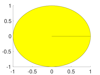
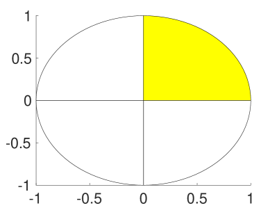
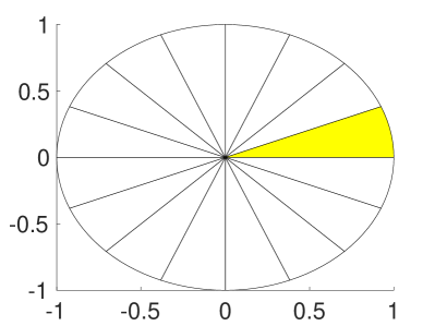
Figure 2: The unit disk $\mathcal{X}\subset\mathbb{R}^{2}$ with the action of the (discrete) rotation groups $\Sigma=C_{n}$, $n=1,4,16,64$. The fundamental domain $\mathcal{X}_{0}$ for each $C_{n}$ is filled with yellow color.

Figure 2 displays an example where $\mathcal{X}$ is the unit disk in $\mathbb{R}^{2}$, and $\Sigma=C_{n},n=1,4,16,64,$ are the discrete rotation groups acting on $\mathcal{X}$; the fundamental domain $\mathcal{X}_{0}$ for each $\Sigma=C_{n}$ is filled with yellow color. We note that the choice of the fundamental domain $\mathcal{X}_{0}$ is not unique. We will slightly abuse the notation $\mathcal{X}=\Sigma\times\mathcal{X}_{0}$ to denote $\mathcal{X}_{0}$ being a fundamental domain of $\mathcal{X}$ under the $\Sigma$-action. We define $T_{0}:\mathcal{X}\to\mathcal{X}_{0}$

$$T_{0}(x)\coloneqq y\in\mathcal{X}_{0},~{}\text{if}~{}y=\sigma x~{}\text{for some}~{}\sigma\in\Sigma,$$ (23)

i.e., $T_{0}$ maps $x\in\mathcal{X}$ to its unique orbit representative in $\mathcal{X}_{0}$. In addition, we denote by $P_{\mathcal{X}_{0}}\in\mathcal{P}(\mathcal{X}_{0})$ the distribution on the fundamental domain $\mathcal{X}_{0}$ induced by a $\Sigma$-invariant distribution $P\in\mathcal{P}_{\Sigma}(\mathcal{X})$ on $\mathcal{X}$; that is,

$$P_{\mathcal{X}_{0}}=(T_{0})_{\sharp}P.$$ (24)

The diameter of $\mathcal{X}\subset\mathbb{R}^{d}$ is defined as

$$\text{diam}(\mathcal{X})=\sup_{x,y\in\mathcal{X}}\|x-y\|_{2}.$$ (25)

Finally, part of our results in Section 4 relies heavily on the concept of covering numbers which we define below.

Definition 3.2 (Covering number).

Let $(\mathcal{X},\rho)$ be a metric space. A subset $S\subset\mathcal{X}$ is called a $\delta$-cover of $\mathcal{X}$ if for any $x\in\mathcal{X}$ there is an $s\in S$ such that $\rho(s,x)\leq\delta$. The $\delta$-covering number of $\mathcal{X}$ is defined as

$$\mathcal{N}(\mathcal{X},\delta,\rho):=\min\left\{\left|S\right|:S\text{ is a }\delta\text{-cover of }\mathcal{X}\right\}.$$

When $\rho(x,y)=\|x-y\|_{2}$ is the Euclidean metric in $\mathbb{R}^{d}$, we abbreviate $\mathcal{N}(\mathcal{X},\delta,\rho)$ as $\mathcal{N}(\mathcal{X},\delta)$.

4 Sample complexity under group invariance

In this section, we outline our main results for the sample complexity of divergence estimation under group invariance. In particular, we focus on three cases: the Wasserstein-1 metric (18), the MMD (19) and the $(f_{\alpha},\Gamma)$-divergence (20). While the convergence rate in the bounds for the Wasserstein-1 metric and the $(f_{\alpha},\Gamma)$-divergence depends on the dimension of the ambient space, that for the MMD case does not. In all the numerical experiments, for simplicity, we choose $X=\{x_{1},x_{2},\cdots,x_{m}\}$ and $Y=\{y_{1},y_{2},\cdots,y_{n}\}$ to sample from the same $\Sigma$-invariant distribution $P=Q$ for easy visualization and clear benchmark.

4.1 Wasserstein-1 metric, $W(P,Q)$

In this section, we set $\Gamma=\text{Lip}_{L}(\mathcal{X})$ to be the set of $L$-Lipschitz functions on $\mathcal{X}$; see Eq. (4). We further assume that the $\Sigma$-actions on $\mathcal{X}$ is $1$-Lipschitz, i.e., $\|\sigma x-\sigma y\|_{2}\leq\|x-y\|_{2},\forall\sigma\in\Sigma,\forall x,y\in\mathcal{X}$, so that $S_{\Sigma}[\Gamma]\subset\Gamma$ (see Lemma A.3 for a proof). Due to Result 3.1, we have $W(P,Q)=W^{\Sigma}(P,Q)$ for $\Sigma$-invariant probability measures $P,Q\in\mathcal{P}_{\Sigma}(\mathcal{X})$.

To convey the main message, we provide a summary of our result in Theorem 4.1 for the sample complexity under group invariance for the Wasserstein-1 metric. The detailed statement and the technical assumption of the theorem as well as its proof are deferred to Section A.1. Readers are referred to Section 3 for the notations.

Theorem 4.1.

Let $\mathcal{X}=\Sigma\times\mathcal{X}_{0}$ be a subset of $\mathbb{R}^{d}$ equipped with the Euclidean distance. Suppose $P,Q\in\mathcal{P}_{\Sigma}(\mathcal{X})$ are $\Sigma$-invariant distributions on $\mathcal{X}$. If the number $m,n$ of samples drawn from $P$ and $Q$ are sufficiently large, then we have with high probability,

1) when $d\geq 2$, for any $s>0$ ,

$$\left|W(P,Q)-W^{\Sigma}(P_{m},Q_{n})\right|$$

$$\quad\leq C\left[\left(\frac{1}{\left|\Sigma\right|m}\right)^{\frac{1}{d+s}}+\left(\frac{1}{\left|\Sigma\right|n}\right)^{\frac{1}{d+s}}\right],$$ (26)

where $C>0$ depends only on $d,s$ and $\mathcal{X}$, and is independent of $m$ and $n$;

2) for $d=1$, we have

$$\left|W(P,Q)-W^{\Sigma}(P_{m},Q_{n})\right|$$

$$\quad\leq C\cdot\text{diam}(\mathcal{X}_{0})\left(\frac{1}{\sqrt{m}}+\frac{1}{\sqrt{n}}\right),$$ (27)

where $C>0$ is an absolute constant independent of $\mathcal{X},\mathcal{X}_{0},m$ and $n$.

Remark 4.2.

In the case for $d\geq 2$, the $s>0$ in Theorem 4.1 means the rate can be arbitrarily close to $-\frac{1}{d}$. If we further assume that $\mathcal{X}_{0}$ is connected, then the bound can be improved to $\left|W(P,Q)-W^{\Sigma}(P_{m},Q_{n})\right|\leq C\left[\left(\frac{1}{\left|\Sigma\right|m}\right)^{\frac{1}{2}}\ln m+\left(\frac{1}{\left|\Sigma\right|n}\right)^{\frac{1}{2}}\ln n\right]$ for $d=2$, and $\left|W(P,Q)-W^{\Sigma}(P_{m},Q_{n})\right|\leq C\left[\left(\frac{1}{\left|\Sigma\right|m}\right)^{\frac{1}{d}}+\left(\frac{1}{\left|\Sigma\right|n}\right)^{\frac{1}{d}}\right]$ for $d\geq 3$, without the dependence of $s$, which matches the rate in (Fournier & Guillin, 2015). See Remark A.7 after Lemma A.6 in the Appendix.

Sketch of the proof. Using the group invariance and the map $T_{0}$ defined in (23), we can transform the i.i.d. samples on $\mathcal{X}$ to i.i.d. samples on $\mathcal{X}_{0}$, which are effectively sampled from $P_{\mathcal{X}_{0}}$ and $Q_{\mathcal{X}_{0}}$ [cf. Eq. (24)]. Hence the supremum after applying the triangle inequality to the error (26) can be taken over $L$-Lipschitz functions defined on the fundamental domain $\mathcal{X}_{0}$, i.e., $\text{Lip}_{L}(\mathcal{X}_{0})$, instead of over the original space $\text{Lip}_{L}(\mathcal{X})$. We further demonstrate in Lemma A.4 that the supremum can be taken over an even smaller function space

$$\mathcal{F}_{0}=\{\gamma\in\text{Lip}_{L}(\mathcal{X}_{0}):\left\lVert\gamma\right\rVert_{\infty}\leq M\}\subset\text{Lip}_{L}(\mathcal{X}_{0}),$$ (28)

with some uniformly bounded $L^{\infty}$-norm $M$ due to the translation-invariance of $\gamma$ in definition (4). Using Dudley’s entropy integral (Bartlett et al., 2017), the error can be bounded in terms of the metric entropy of $\mathcal{F}_{0}$ with $m$ i.i.d. samples,

$$\inf_{\alpha>0}\left\{8\alpha+\frac{24}{\sqrt{m}}\int_{\alpha}^{M}\sqrt{\ln\mathcal{N}(\mathcal{F}_{0},\delta,\left\lVert\cdot\right\rVert_{\infty})}\mathop{}\!\mathrm{d}{\delta}\right\}.$$ (29)

For $d\geq 2$, we establish the relations between the metric entropy, $\ln\mathcal{N}(\mathcal{F}_{0},\delta,\left\lVert\cdot\right\rVert_{\infty})$, of $\mathcal{F}_{0}$ and the covering numbers of $\mathcal{X}_{0}$ and $\mathcal{X}$ via Lemma A.6 and Lemma A.8:

$$\ln\mathcal{N}(\mathcal{F}_{0},\delta,\left\lVert\cdot\right\rVert_{\infty}) \leq\mathcal{N}(\mathcal{X}_{0},\frac{c_{2}\delta}{L})\ln(\frac{c_{1}M}{\delta}),$$ (30)

$$\frac{\mathcal{N}(\mathcal{X}_{0},\delta)}{\mathcal{N}(\mathcal{X},\delta)} \leq\frac{1}{\left|\Sigma\right|},~{}\text{for small enough}~{}\delta,$$ (31)

which yields a factor in terms of the group size $\left|\Sigma\right|$ in Eq. (26). The dominant term of the bound based on the singularity of the entropy integral at $\alpha=0$ is shown in Eq. (26). For $d=1$, the entropy integral is not singular at the origin, and we bound the covering number of $\mathcal{F}_{0}$ by $\text{diam}(\mathcal{X}_{0})$ instead. The probability bound is from the application of the McDiarmid’s inequality.

Remark 4.3.

Even though we present in Theorem 4.1 only the dominant terms showing the rate of convergence for the estimator, our result for sample complexity is actually non-asymptotic. See Theorem A.2 in Section A.1 for a complete description of the result.

Remark 4.4.

When $|\Sigma|=1$, i.e., no group symmetry is leveraged in the divergence estimation, our result reduces to the case considered in, e.g., (Sriperumbudur et al., 2012), for general distributions $P,Q\in\mathcal{P}_{\Sigma}(\mathcal{X})=\mathcal{P}(\mathcal{X})$.

Remark 4.5.

The factor $\text{diam}(\mathcal{X}_{0})$ in the case for $d=1$ is not necessarily directly related to the group size $\left|\Sigma\right|$. We refer to Example 4.6 below and its explanation in Remark A.10 for cases where we can achieve a factor of $\left|\Sigma\right|^{-1}$ in the rate.

Example 4.6.

Let $\mathcal{X}=[0,1)$ and $\Gamma=\text{Lip}_{L}\left([0,1)\right)$, i.e., $d=1$. We consider the $\Sigma$-actions on $\mathcal{X}$ generated by the translation $x\mapsto(x+\frac{1}{r})\mod 1$, where $r=1,4,16,64,256$, so that $|\Sigma|=r$ is the group size. We draw samples $x_{i}\sim P=Q\in\mathcal{P}_{\Sigma}(\mathcal{X})$ on $\mathcal{X}$ in the following way: $x_{i}=r^{-1}\xi^{1/3}_{i}+\eta_{i}$, where $\xi_{i}$ are i.i.d. uniformly distributed random variables on $[0,1)$ and $\eta_{i}$ take values over $\{0,\frac{1}{r},\dots,\frac{r-1}{r}\}$ with equal probabilities. One can easily verify that $P=Q$ are indeed $\Sigma$-invariant. The numerical results for the empirical estimation of $W(P,Q)=0$ using $W^{\Sigma}(P_{n},Q_{n})$ with different group size $|\Sigma|=r$, $r=1,4,16,64,256$, are shown in the left panel of Figure 3. One can clearly observe a significant improvement of the estimator as the group size $|\Sigma|$ increases. Furthermore, the right panel of Figure 3 displays the ratios between the adjacent curves, all of which converge to 4, which is the ratio between the consecutive group size. This matches our calculation in Remark A.10; see also Remark 4.5.

Example 4.7.

We let $\mathcal{X}=\mathbb{R}^{2}$, i.e., $d=2$. The probability distributions $P=Q$ are the mixture of 8 Gaussians centered at $\left(\cos(\frac{2\pi r}{8}),\sin(\frac{2\pi r}{8})\right)$, $r=0,1,\dots,7$, with the same covariance. The distribution has $C_{8}$-rotation symmetry, but we pretend that it is only $C_{1},C_{2}$ and $C_{4}$; that is, the $\Sigma$ used in the empirical estimation $W^{\Sigma}(P_{m},Q_{n})$ does not reflect the entire invariance structure. Even though in this case the domain $\mathcal{X}$ is unbounded, which is beyond our theoretical assumptions, we can still see in Figure 4 that as we increase the group size $|\Sigma|$ in the computation of $W^{\Sigma}(P_{m},Q_{n})$, fewer samples are needed to reach the same accuracy level in the approximation. The ratios between adjacent curves in this case are slightly above the predicted value $\sqrt{2}\approx 1.414$ according to our theory (see Remark 4.2), suggesting that the complexity bound could be further improved. For instance, in (Sriperumbudur et al., 2012), a logarithmic correction term can be revealed for $d=2$ after a more thorough analysis.

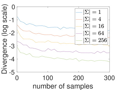
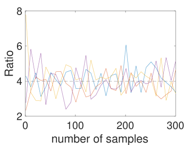
Figure 3: Left: the Wasserstein-1 distance with different group sizes on $[0,1)$, averaged over 10 replicas. Right: the ratio of the average of the Wasserstein-1 distance between different group sizes: $\left|\Sigma\right|=1$ over $\left|\Sigma\right|=4$ (blue), $\left|\Sigma\right|=4$ over $\left|\Sigma\right|=16$ (red), $\left|\Sigma\right|=16$ over $\left|\Sigma\right|=64$ (orange), $\left|\Sigma\right|=64$ over $\left|\Sigma\right|=256$ (purple). The black horizontal dashed line refers to the ratio equal to 4, which is the value theoretically predicted in Theorem 4.1 for $d=1$. See Example 4.6 and Remark A.10 for the detail.

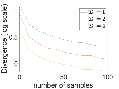
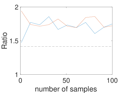
Figure 4: Left: The Wasserstein-1 distance assuming different group sizes in $\mathbb{R}^{2}$, averaged over 10 replicas. Right: the ratio of the average of the Wasserstein-1 distance between different group sizes: $\left|\Sigma\right|=1$ over $\left|\Sigma\right|=2$ (blue), $\left|\Sigma\right|=2$ over $\left|\Sigma\right|=4$ (red). The black horizontal dashed line refers to the ratio equal to $\sqrt{2}$, which is the value theoretically predicted in Theorem 4.1 for $d=2$. The ratios are slightly above the reference line, suggesting that the complexity bound could be further improved. See Example 4.7 and Remark 4.2 for the detail.

4.2 Lipschitz-regularized $\alpha$-divergence, $D_{f_{\alpha}}^{\Gamma}(P\|Q)$

The Lipschitz-regularized $\alpha$-divergence is used in the symmetry-preserving GANs (Birrell et al., 2022c), where it allowed them to systematically include symmetries and gave a vastly improved performance on real data sets. The space $\Gamma$ in this section is always set to $\Gamma=\text{Lip}_{L}(\mathcal{X})$; see Eq. (7). We only consider $\alpha>1$, as the case when $0<\alpha<1$ can be derived in a similar manner. For $\alpha>1$, the Legendre transform of $f_{\alpha}$, which is defined in (7), is

$$f_{\alpha}^{*}(y)=\left(\alpha^{-1}(\alpha-1)^{\frac{\alpha}{\alpha-1}}y^{\frac{\alpha}{\alpha-1}}+\frac{1}{\alpha(\alpha-1)}\right)\mathbf{1}_{y>0}.$$

We provide a theorem for the sample complexity for the $(f_{\alpha},\Gamma)$-divergence under group invariance, whose detailed statement and proof can be found in Section A.2. We note that this is a new sample complexity result for the $(f_{\alpha},\Gamma)$-divergence even without the group structure, which is still missing in the literature.

Theorem 4.8.

Let $\mathcal{X}=\Sigma\times\mathcal{X}_{0}$ be a subset of $\mathbb{R}^{d}$ equipped with the Euclidean distance. Let $f_{\alpha}(x)=\frac{x^{\alpha}-1}{\alpha(\alpha-1)}$, $\alpha>1$ and $\Gamma=\text{Lip}_{L}(\mathcal{X})$. Suppose $P$ and $Q$ are $\Sigma$-invariant distributions on $\mathcal{X}$. If the number of samples $m,n$ drawn from $P$ and $Q$ are sufficiently large, we have with high probability,

1) when $d\geq 2$, for any $s>0$ ,

$$\left|D_{f_{\alpha}}^{\Gamma}(P\|Q)-D_{f_{\alpha}}^{\Gamma_{\Sigma}}(P_{m}\|Q_{n})\right|$$

$$\leq C_{1}\left(\frac{1}{\left|\Sigma\right|m}\right)^{\frac{1}{d+s}}+C_{2}\left(\frac{1}{\left|\Sigma\right|n}\right)^{\frac{1}{d+s}},$$ (32)

where $C_{1}$ depends only on $d,s$ and $\mathcal{X}$; $C_{2}$ depends only on $d,s$, $\mathcal{X}$ and $\alpha$; both $C_{1}$ and $C_{2}$ are independent of $m$ and $n$;

2) for $d=1$, we have

$$\left|D_{f_{\alpha}}^{\Gamma}(P\|Q)-D_{f_{\alpha}}^{\Gamma_{\Sigma}}(P_{m}\|Q_{n})\right|$$

$$\quad\leq\text{diam}(\mathcal{X}_{0})\left(\frac{C_{1}}{\sqrt{m}}+\frac{C_{2}}{\sqrt{n}}\right),$$ (33)

where $C_{1}$ and $C_{2}$ are independent of $\mathcal{X}_{0}$, $m$ and $n$; $C_{2}$ depends on $\alpha$.

Sketch of the proof. The idea is similar to the proof of Theorem 4.1. The only difference is that we need to tackle the $f_{\alpha}^{*}(\gamma)$ term separately, since it is not translation-invariant in $\gamma$. Using the equivalent form (8), we can obtain a different Lipschitz constant associated with $f_{\alpha}^{*}$, as well as a different $L^{\infty}$ bound $M$ than that in Eq. (28) by Lemma A.12. This results in the $\alpha$ dependence for $C_{2}$.

4.3 Maximum mean discrepancy, $\text{MMD}(P,Q)$

Though one can utilize the results on the covering number of the unit ball of a reproducing kernel Hilbert space, e.g. (Zhou, 2002; Kühn, 2011), to derive the sample complexity bounds that depend on the dimension $d$, we provide a dimension-independent bound as in (Gretton et al., 2012) without the use of the covering numbers. In the MMD case, we let $B_{\mathcal{H}}$ represent the unit ball in some reproducing kernel Hilbert space (RKHS) $\mathcal{H}$ on $\mathcal{X}$; see Eq. (5). In addition, we make the following assumptions for the kernel $k(x,y)$.

Assumption 4.9.

The kernel $k(x,y)$ for $\mathcal{H}$ satisfies

• $k(x,y)\geq 0$ and $k(\sigma(x),\sigma(y))=k(x,y),\forall{\sigma}\in\Sigma,x,y\in\mathcal{X}$;

• Let $K:=\max_{x,y\in\mathcal{X}}k(x,y)$, then $k(x,y)=K$ if and only if $x=y$;

• There exists $c_{\Sigma,k}\in(0,1)$ such that for any $\sigma\in\Sigma$ and $\sigma$ is not the identity element and $x\in\mathcal{X}_{0}$, we have $k(\sigma x,x)\leq c_{\Sigma,k}K$.

Intuitively, the third condition in 4.9 suggests uniform decay of the kernel on the group orbits. See Remark 4.12 and Example 4.13 for more details and a related example.

From Lemma C.1 in (Birrell et al., 2022c), we know $S_{\Sigma}[\Gamma]\subset\Gamma$ by the first assumption. Below is an abbreviated result for the sample complexity for the MMD, whose detailed statement and proof can be found in Section A.3.

Theorem 4.10.

Let $\mathcal{X}=\Sigma\times\mathcal{X}_{0}$ be a subset of $\mathbb{R}^{d}$. $\mathcal{H}$ is a RKHS on $\mathcal{X}$ whose kernel satisfies 4.9. Suppose $P$ and $Q$ are $\Sigma$-invariant distributions on $\mathcal{X}$. Then for $m,n$ sufficiently large, we have with high probability,

$$\left|\text{MMD}(P,Q)-\text{MMD}^{\Sigma}(P_{m},Q_{n})\right|$$

$$\quad<O\left(C_{\Sigma,k}\left(\frac{1}{\sqrt{m}}+\frac{1}{\sqrt{n}}\right)\right),$$ (34)

where $C_{\Sigma,k}=\sqrt{\frac{1+c_{\Sigma,k}(\left|\Sigma\right|-1)}{\left|\Sigma\right|}}$, and $c_{\Sigma,k}$ is the constant in 4.9.

Sketch of the proof. Based on Result 3.1, we use the equality $\text{MMD}^{\Sigma}(P_{m},Q_{n})=\text{MMD}(S^{\Sigma}[P_{m}],S^{\Sigma}[Q_{n}])$ to expand the divergence over all the orbit elements. The error bound is controlled in terms of the Rademacher average, whose supremum is attained at some known witness function due to the structure of the RKHS using Lemma A.14. Since the Rademacher average is estimated without covering numbers, the rate is independent of the dimension $d$. Then we use the decay of the kernel to obtain the bound.

Remark 4.11.

When $\left|\Sigma\right|=1$, the proof is reduced to that in (Sriperumbudur et al., 2012).

Remark 4.12.

Unlike the cases for the Wasserstein metric and the Lipschitz-regularized $\alpha$-divergence in Theorem 4.1 and Theorem 4.8, the improvement of the sample complexity under group symmetry for MMD (measured by $C_{\Sigma,k}$ in Theorem 4.10) depends on not only the group size $|\Sigma|$ but also the kernel $k(x,y)$. For a fixed $\mathcal{X}$ and kernel $k(x,y)$, simply increasing the group size $\left|\Sigma\right|$ does not necessarily lead to a reduced sample complexity beyond a certain threshold; see the first four subfigures in Figure 5. However, we show in Example 4.13 below that, by adaptively picking a suitable kernel $k$ depending on the group size $\left|\Sigma\right|$, one can obtain an improvement in sample complexity by $C_{\Sigma,k}\approx\frac{1}{\sqrt{\left|\Sigma\right|}}$ for arbitrarily large $\left|\Sigma\right|$.

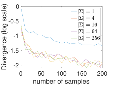
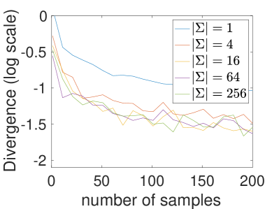
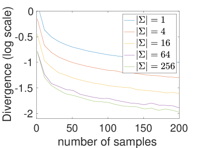
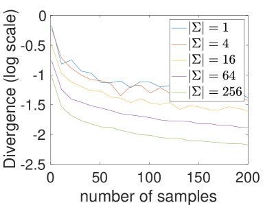
Figure 5: MMD simulations with Gaussian kernels $k_{s}(x,y)=e^{-\frac{\left\lVert x-y\right\rVert_{2}^{2}}{2s^{2}}}$. From left to right, top to bottom: $s=\frac{2\pi}{1\times 6}$, $s=\frac{2\pi}{4\times 6}$, $s=\frac{2\pi}{16\times 6}$, $s=\frac{2\pi}{64\times 6}$, $s=\frac{2\pi}{6\left|\Sigma\right|}$. The first four subfigures (top two rows) show that the Gaussian kernel with a fixed bandwidth $s>0$ satisfies the third condition in 4.9 up to a group size of $\left|\Sigma\right|=l,l=1,4,16,64$, and thus an improvement of sample complexity of order $C_{\Sigma,k}\approx\left|\Sigma\right|^{-1/2}$ persists till $\left|\Sigma\right|=l$; when $\left|\Sigma\right|>l$, no further reduction in sample complexity can be observed. The last subfigure demonstrates that with an adaptive bandwidth $s$ inversely scaled with $\left|\Sigma\right|$, nonstop improvement of the sample complexity can be achieved as the group size $\left|\Sigma\right|$ increases. See Example 4.13 for the detail and explanations.

Example 4.13.

Let $\mathcal{X}=\{(r\cos\theta,r\sin\theta)\in\mathbb{R}^{2}:r\in[0,1],\theta\in[0,2\pi)\}$ be the unit disk centered at the origin, and let $k_{s}(x,y)=e^{-\frac{\left\lVert x-y\right\rVert_{2}^{2}}{2s^{2}}}$, $x,y\in\mathcal{X}$, be the Gaussian kernel. Consider the group actions generated by a rotation (with respect to the origin) of $\frac{2\pi}{l}$, $l=1,4,16,64,256$, so that $|\Sigma|=l$ is the group size. The fundamental domain $\mathcal{X}_{0}$ under the $\Sigma$-action is $\mathcal{X}_{0}=[0,1]\times[0,\frac{2\pi}{l})$ (see Figure 2 for a visual illustration). We draw samples $x_{i}\sim P=Q\in\mathcal{P}_{\Sigma}(\mathcal{X})$ in the following way,

$$x_{i}=\sqrt{\xi}_{i}\left(\cos\left[\frac{2\pi}{l}\theta^{1/3}_{i}+\eta_{i}\frac{2\pi}{l}\right],\sin\left[\frac{2\pi}{l}\theta^{1/3}_{i}+\eta_{i}\frac{2\pi}{l}\right]\right)$$

where $\xi_{i}$ and $\theta_{i}$ are i.i.d. uniformly distributed random variables on $[0,1)$ and $\eta_{i}$ take values over $\{0,\frac{1}{l},\dots,\frac{l-1}{l}\}$ with equal probabilities. We select the kernel bandwidth $s>0$ in different ways:

• Fixed $s$ with changing group size $\left|\Sigma\right|=l$. We intuitively follow the “three-sigma rule” in the argument direction to pick different $s$. Since the angle of each sector is $\frac{2\pi}{l}$, we select $s=\frac{2\pi}{6l}$, $l=1,4,16,64$. Smaller bandwidth $s$ corresponds to faster decay of the kernel $k_{s}(x,y)$, such that for a fixed bandwidth $s=\frac{2\pi}{6l}$, the third condition in 4.9 is satisfied with a small $c_{k}$ for any group $\Sigma$ such that $\left|\Sigma\right|\leq l$, i.e., $C_{\Sigma,k}\approx\left|\Sigma\right|^{-1/2}$. On the other hand, it is difficult to observe the improvement by further increasing the group size $\left|\Sigma\right|$ beyond $\left|\Sigma\right|>l$, since the third condition in 4.9 is not satisfied with any uniformly small $c$. See the top two rows in Figure 5 for the results for $s=\frac{2\pi}{l\times 6}$, $l=1,4,16,64$. Notice that the sample complexity improvement stops right at $|\Sigma|=l$, perfectly matching our theoretical result Theorem 4.10.

• $s$ inversely scales with $\left|\Sigma\right|$, i.e., $s=\frac{2\pi}{6\left|\Sigma\right|}$. Unlike the fixed $s$ discusses previously, with these adaptive selections of kernels, we can observe nonstop improvement of the sample complexity as the group size $\left|\Sigma\right|$ increases; see the last row of Figure 5. This numerical result is explained by the third condition in 4.9; that is, in order to continuously observe the benefit from the increasing group size $\left|\Sigma\right|$, we need to have a faster decay in the kernel $k_{s}$ (i.e., smaller $s$) so that $c_{\Sigma,k_{s}}$ is uniformly small for all $\left|\Sigma\right|$.

Remark 4.14.

The bound provided in Theorem 4.10 for the MMD case is almost sharp in the sense that, by a direct calculation, one can obtain that

$$\frac{E_{\mathcal{X}}\text{MMD}^{\Sigma}(P,P_{n})^{2}}{E_{\mathcal{X}}\text{MMD}(P,P_{n})^{2}}\approx C_{\Sigma,k}^{2},$$

if the kernel bandwidth $s\propto\frac{\sqrt{2c_{\Sigma,k}}\pi}{\left|\Sigma\right|}$.

5 Conclusion and future work

We provide rigorous analysis to quantify the reduction in sample complexity for variational divergence estimations between group-invariant distributions. We obtain a reduction on the error bound by a power of the group size. The exponent on the group size depends on the ambient dimension for the Wasserstein-1 metric and the Lipschitz-regularized $\alpha$-divergence; that exponent, however, is independent of the ambient dimension for the MMD with a proper choice of the kernel.

This work also motivates some possible future directions. For the Wasserstein-1 metric in $\mathbb{R}^{2}$, one could potentially derive a sharper bound in terms of the group size. For the MMD with Gaussian kernels, it is worth investigating how to choose the bandwidth to make as much use of the group structure as possible. Further applications of the theories on machine learning, such as neural generative models or neural estimations of divergence under symmetry, are also expected.

Appendix A Theorems and Proofs

In this section, we provide detailed statements of the theorems introduced in the main text as well as their proofs.

A.1 Wasserstein-1 metric

Assumption A.1.

Let $\mathcal{X}=\Sigma\times\mathcal{X}_{0}\subset\mathbb{R}^{d}$. Assume that there exists some $\delta_{0}>0$ such that

1. $\left\lVert\sigma(x)-\sigma^{\prime}(x^{\prime})\right\rVert_{2}>2\delta_{0}$, $\forall x,x^{\prime}\in\mathcal{X}_{0},\sigma\neq\sigma^{\prime}\in\Sigma$; and

2. $\left\lVert\sigma(x)-\sigma(x^{\prime})\right\rVert_{2}\geq\left\lVert x-x^{\prime}\right\rVert_{2}$, $\forall x,x^{\prime}\in\mathcal{X}_{0},\sigma\in\Sigma$,

where $\|\cdot\|_{2}$ is the Euclidean norm on $\mathbb{R}^{d}$.

Example 4.6 provides a simple example when this assumption holds.

Theorem A.2.

Let $\mathcal{X}=\Sigma\times\mathcal{X}_{0}$ be a subset of $\mathbb{R}^{d}$ satisfying the conditions in Assumption A.1. Suppose $P$ and $Q$ are $\Sigma$-invariant probability measures on $\mathcal{X}$.

1) If $d\geq 2$, then for any $s>0,\epsilon>0$ and $m,n$ sufficiently large, we have with probability at least $1-\epsilon$,

$$\left|W(P,Q)-W^{\Sigma}(P_{m},Q_{n})\right| \leq\left(8+\frac{24}{(\frac{d+s}{2}-1)}\right)\left[\left(\frac{9D_{\mathcal{X},L}^{2}}{\left|\Sigma\right|m}\right)^{\frac{1}{d+s}}+\left(\frac{9D_{\mathcal{X},L}^{2}}{\left|\Sigma\right|n}\right)^{\frac{1}{d+s}}\right]$$

$$\quad+\bar{D}_{\mathcal{X}_{0},L}\left(\frac{24}{\sqrt{m}}+\frac{24}{\sqrt{n}}\right)+L\cdot\text{diam}(\mathcal{X}_{0})\sqrt{\frac{2(m+n)}{mn}\ln\frac{1}{\epsilon}},$$

where $D_{\mathcal{X},L}$ depends only on $\mathcal{X}$ and $L$; $\bar{D}_{\mathcal{X}_{0},L}$ depends only on $\mathcal{X}_{0}$ and $L$, and is increasing in $\mathcal{X}_{0}$, i.e., $\bar{D}_{A_{1},L}\leq\bar{D}_{A_{2},L}$ for $A_{1}\subset A_{2}$;
2) If $d=1$, then for any $\epsilon>0$ and $m,n$ sufficiently large, we have with probability at least $1-\epsilon$,

$$\left|W(P,Q)-W^{\Sigma}(P_{m},Q_{n})\right| \leq cL\cdot\text{diam}(\mathcal{X}_{0})\left(\frac{1}{\sqrt{m}}+\frac{1}{\sqrt{n}}\right)+L\cdot\text{diam}(\mathcal{X}_{0})\sqrt{\frac{2(m+n)}{mn}\ln\frac{1}{\epsilon}},$$

where $c>0$ is an absolute constant independent of $\mathcal{X}$ and $\mathcal{X}_{0}$.

Before proving this theorem, we have the following lemmas.

Lemma A.3.

Suppose the $\Sigma$-actions on $\mathcal{X}$ are $1$-Lipschitz, i.e., $\left\lVert\sigma x-\sigma y\right\rVert_{2}\leq\left\lVert x-y\right\rVert_{2}$ for any $x,y\in\mathcal{X}$ and $\sigma\in\Sigma$, then we have $S_{\Sigma}[\Gamma]\subset\Gamma$, where $\Gamma=\text{Lip}_{L}(\mathcal{X})$.

Proof.

For any $x,y\in\mathcal{X}$ and $f\in\Gamma$, we have

$$\left|S_{\Sigma}(f)(x)-S_{\Sigma}(f)(y)\right| =\left|\frac{1}{\left|\Sigma\right|}\sum_{\sigma\in\Sigma}f\left(\sigma x\right)-\frac{1}{\left|\Sigma\right|}\sum_{\sigma\in\Sigma}f\left(\sigma y\right)\right|$$

$$\leq\frac{1}{\left|\Sigma\right|}\sum_{\sigma\in\Sigma}\left|f\left(\sigma x\right)-f\left(\sigma y\right)\right|$$

$$\leq\frac{1}{\left|\Sigma\right|}\sum_{\sigma\in\Sigma}L\left\lVert\sigma x-\sigma y\right\rVert_{2}$$

$$\leq\frac{1}{\left|\Sigma\right|}\sum_{\sigma\in\Sigma}L\left\lVert x-y\right\rVert_{2}$$

$$=L\left\lVert x-y\right\rVert_{2}.$$

Therefore, we have $S_{\Sigma}(f)\in\Gamma$. ∎

Lemma A.4.

For any $\gamma\in\text{Lip}_{L}(\mathcal{X}_{0})$, there exists $\nu\in\mathbb{R}$, such that $\left\lVert\gamma+\nu\right\rVert_{\infty}\leq L\cdot\text{diam}(\mathcal{X}_{0})$.

Proof.

Suppose $\gamma\in\text{Lip}_{L}(\mathcal{X}_{0})$ and $\left\lVert\gamma(x)\right\rVert_{\infty}>L\cdot\text{diam}(\mathcal{X}_{0})$. Without loss of generality, we can assume $\sup_{x\in\mathcal{X}_{0}}\gamma(x)>L\cdot\text{diam}(\mathcal{X}_{0})$. Since $\gamma$ is $L$-Lipschitz on $\mathcal{X}_{0}$, we have $\sup_{x\in\mathcal{X}_{0}}\gamma(x)-\inf_{x\in\mathcal{X}_{0}}\gamma(x)\leq L\cdot\text{diam}(\mathcal{X}_{0})$, so that

$$\inf_{x\in\mathcal{X}_{0}}\gamma(x)\geq\sup_{x\in\mathcal{X}_{0}}\gamma(x)-L\cdot\text{diam}(\mathcal{X}_{0})>0.$$

Hence we can select $\nu=-\frac{\inf_{x\in\mathcal{X}_{0}}\gamma(x)}{2}$, so that $\left\lVert\gamma+\nu\right\rVert_{\infty}<\left\lVert\gamma\right\rVert_{\infty}$. ∎

We provide a variant of the Dudley’s entropy integral as well as its proof for completeness.

Lemma A.5.

Suppose $\mathcal{F}$ is a family of functions mapping the metric space $(\mathcal{X},\rho)$ to $[-M,M]$ for some $M>0$. Also assume that $0\in\mathcal{F}$ and $\mathcal{F}=-\mathcal{F}$. Let $\xi=\{\xi_{1},\dots,\xi_{m}\}$ be a set of independent random variables that take values on $\{-1,1\}$ with equal probabilities, $i=1,\dots,m$. $x_{1},x_{2},\dots,x_{m}\in\mathcal{X}$. Then we have

$$E_{\xi}\sup_{f\in\mathcal{F}}\left|\frac{1}{m}\sum_{i=1}^{m}\xi_{i}f(x_{i})\right|\leq\inf_{\alpha>0}4\alpha+\frac{12}{\sqrt{m}}\int_{\alpha}^{M}\sqrt{\ln\mathcal{N(\mathcal{F},\delta,\left\lVert\cdot\right\rVert_{\infty})}}\mathop{}\!\mathrm{d}{\delta}.$$

The proof of Lemma A.5 is standard using the dyadic path., e.g. see the proof of Lemma A.5. in (Bartlett et al., 2017).

Proof.

Let $N$ be an arbitrary positive integer and $\delta_{k}=M2^{-(k-1)}$, $k=1,\dots,N$. Let $V_{k}$ be the cover achieving $\mathcal{N}(\mathcal{F},\delta_{k},\left\lVert\cdot\right\rVert_{\infty})$ and denote $\left|V_{k}\right|=\mathcal{N}(\mathcal{F},\delta_{k},\left\lVert\cdot\right\rVert_{\infty})$. For any $f\in\mathcal{F}$, let $\pi_{k}(f)\in V_{k}$, such that $\left\lVert f-\pi_{k}(f)\right\rVert_{\infty}\leq\delta_{k}$. We have

$$E_{\xi}\sup_{f\in\mathcal{F}}\left|\frac{1}{m}\sum_{i=1}^{m}\xi_{i}f(x_{i})\right|$$

$$\leq E_{\xi}\sup_{f\in\mathcal{F}}\left|\frac{1}{m}\sum_{i=1}^{m}\xi_{i}\left(f(x_{i})-\pi_{N}(f)(x_{i})\right)\right|+\sum_{j=1}^{N-1}E_{\xi}\sup_{f\in\mathcal{F}}\left|\frac{1}{m}\sum_{i=1}^{m}\xi_{i}\left(\pi_{j+1}(f)(x_{i})-\pi_{j}(f)(x_{i})\right)\right|$$

$$\quad+E_{\xi}\sup_{f\in\mathcal{F}}\left|\frac{1}{m}\sum_{i=1}^{m}\xi_{i}\pi_{1}(f)(x_{i})\right|.$$

The first on the right hand side is bounded by $\delta_{N}$. Note that we can choose $V_{1}=\{0\}$, so that $\pi_{1}(f)$ is the zero function. For each $j$, let $W_{j}=\{\pi_{j+1}(f)-\pi_{j}(f):f\in\mathcal{F}\}$. We have $\left|W_{j}\right|\leq\left|V_{j+1}\right|\left|V_{j}\right|\leq\left|V_{j+1}\right|^{2}$. Then we have

$$\sum_{j=1}^{N-1}E_{\xi}\sup_{f\in\mathcal{F}}\left|\frac{1}{m}\sum_{i=1}^{m}\xi_{i}\left(\pi_{j+1}(f)(x_{i})-\pi_{j}(f)(x_{i})\right)\right|=\sum_{j=1}^{N-1}E_{\xi}\sup_{w\in W_{j}}\left|\frac{1}{m}\sum_{i=1}^{m}\xi_{i}w(x_{i})\right|.$$

In addition, we have

$$\sup_{w\in W_{j}}\sqrt{\sum_{i=1}^{m}w(x_{i})^{2}}$$

$$=\sup_{f\in\mathcal{F}}\sqrt{\sum_{i=1}^{m}\left(\pi_{j+1}(f)(x_{i})-\pi_{j}(f)(x_{i})\right)^{2}}$$

$$\leq\sup_{f\in\mathcal{F}}\sqrt{\sum_{i=1}^{m}\left(\pi_{j+1}(f)(x_{i})-f(x_{i})\right)^{2}}+\sup_{f\in\mathcal{F}}\sqrt{\sum_{i=1}^{m}\left(f(x_{i})-\pi_{j}(f)(x_{i})\right)^{2}}$$

$$\leq\sqrt{m\cdot\delta_{j+1}^{2}}+\sqrt{m\cdot\delta_{j}^{2}}$$

$$=\sqrt{m}(\delta_{j+1}+\delta_{j})$$

$$=3\sqrt{m}\delta_{j+1}.$$

By the Massart finite class lemma (see, e.g. (Mohri et al., 2018)), we have

$$E_{\xi}\sup_{w\in W_{j}}\left|\frac{1}{m}\sum_{i=1}^{m}\xi_{i}w(x_{i})\right|\leq\frac{3\sqrt{m}\delta_{j+1}\sqrt{2\ln\left|W_{j}\right|}}{m}\leq\frac{6\delta_{j+1}\sqrt{\ln\left|V_{j+1}\right|}}{\sqrt{m}}.$$

Therefore,

$$E_{\xi}\sup_{f\in\mathcal{F}}\left|\frac{1}{m}\sum_{i=1}^{m}\xi_{i}f(x_{i})\right| \leq\delta_{N}+\frac{6}{\sqrt{m}}\sum_{j=1}^{N-1}\delta_{j+1}\sqrt{\ln\mathcal{N}(\mathcal{F},\delta_{j+1},\left\lVert\cdot\right\rVert_{\infty})}$$

$$\leq\delta_{N}+\frac{12}{\sqrt{m}}\sum_{j=1}^{N}(\delta_{j}-\delta_{j+1})\sqrt{\ln\mathcal{N}(\mathcal{F},\delta_{j},\left\lVert\cdot\right\rVert_{\infty})}$$

$$\leq\delta_{N}+\frac{12}{\sqrt{m}}\int_{\delta_{N+1}}^{M}\sqrt{\ln\mathcal{N}(\mathcal{F},\delta,\left\lVert\cdot\right\rVert_{\infty})}\mathop{}\!\mathrm{d}{\delta}.$$

Finally, select any $\alpha\in(0,M)$ and let $N$ be the largest integer with $\delta_{N+1}>\alpha$, (implying $\delta_{N+2}\leq\alpha$ and $\delta_{N}=4\delta_{N+2}\leq 4\alpha$), so that

$$\delta_{N}+\frac{12}{\sqrt{m}}\int_{\delta_{N+1}}^{M}\sqrt{\ln\mathcal{N}(\mathcal{F},\delta_{j},\left\lVert\cdot\right\rVert_{\infty})}\mathop{}\!\mathrm{d}{\delta}\leq 4\alpha+\frac{12}{\sqrt{m}}\int_{\alpha}^{M}\sqrt{\ln\mathcal{N}(\mathcal{F},\delta,\left\lVert\cdot\right\rVert_{\infty})}\mathop{}\!\mathrm{d}{\delta}.$$

∎

We can easily extend Lemma 6 in (Gottlieb et al., 2017) to the following lemma by meshing on the range $[-M,M]$ rather than $[0,1]$.

Lemma A.6.

Let $\mathcal{F}$ be the family of $L$-Lipschitz functions mapping the metric space $(\mathcal{X},\left\lVert\cdot\right\rVert_{2})$ to $[-M,M]$ for some $M>0$. Then we have

$$\mathcal{N}(\mathcal{F},\delta,\left\lVert\cdot\right\rVert_{\infty})\leq(\frac{c_{1}M}{\delta})^{\mathcal{N}(\mathcal{X},\frac{c_{2}\delta}{L})},$$

where $c_{1}\geq 1$ and $c_{2}\leq 1$ are some absolute constants not depending on $\mathcal{X}$, $M$, and $\delta$.

Remark A.7.

If $\mathcal{X}$ is connected, then the bound can be improved to $\mathcal{N}(\mathcal{F},\delta,\left\lVert\cdot\right\rVert_{\infty})\leq e^{\mathcal{N}(\mathcal{X},\frac{c_{2}\delta}{L})}$ by the result in (Kolmogorov, 1961).

Lemma A.8 (Theorem 3 in (Sokolic et al., 2017)).

Assume that $\mathcal{X}=\Sigma\times\mathcal{X}_{0}$. If for some $\delta>0$ we have
1) $\left\lVert\sigma(x)-\sigma^{\prime}(x^{\prime})\right\rVert_{2}>2\delta$, $\forall x,x^{\prime}\in\mathcal{X}_{0},\sigma\neq\sigma^{\prime}\in\Sigma$; and
2) $\left\lVert\sigma(x)-\sigma(x^{\prime})\right\rVert_{2}\geq\left\lVert x-x^{\prime}\right\rVert_{2}$, $\forall x,x^{\prime}\in\mathcal{X}_{0},\sigma\in\Sigma$,
then we have

$$\frac{\mathcal{N}(\mathcal{X}_{0},\delta)}{\mathcal{N}(\mathcal{X},\delta)}\leq\frac{1}{\left|\Sigma\right|}.$$

In addition, we provide the following lemma for the scaling of covering numbers.

Lemma A.9.

Let $\mathcal{X}$ be a subset of $\mathbb{R}^{d}$ and $\bar{\delta}>0$. Then there exists a constant $C_{d,\bar{\delta}}$ that depends on $d$ and $\bar{\delta}$ such that for $\delta\in(0,1)$ we have

$$\mathcal{N}(\mathcal{X},\delta)\leq C_{d,\bar{\delta}}\cdot\frac{\mathcal{N}(\mathcal{X},\bar{\delta})}{\delta^{d}}.$$

Proof.

Let $N:=\mathcal{N}(\mathcal{X},\bar{\delta})$. Then $\mathcal{X}$ can be covered by $N$ balls with radius $\bar{\delta}$. From Proposition 4.2.12 in (Vershynin, 2018), we know that each ball with radius $\bar{\delta}$ can be covered by $\frac{(\bar{\delta}+\delta/2)^{d}}{(\delta/2)^{d}}$ balls with radius $\delta$. This implies that $\mathcal{X}$ can be covered by $N\cdot\frac{(\bar{\delta}+\delta/2)^{d}}{(\delta/2)^{d}}$ balls with radius $\delta$, so that $\mathcal{N}^{\text{ext}}(\mathcal{X},\delta)\leq N\cdot\frac{(\bar{\delta}+\delta/2)^{d}}{(\delta/2)^{d}}$, where $\mathcal{N}^{\text{ext}}(\mathcal{X},\delta)$ is the exterior covering number of $\mathcal{X}$ with radius $\delta$. Therefore, $\mathcal{N}(\mathcal{X},\delta)\leq\mathcal{N}^{\text{ext}}(\mathcal{X},\delta/2)\leq N\cdot\frac{(\bar{\delta}+\delta/4)^{d}}{(\delta/4)^{d}}=N\cdot(\frac{4\bar{\delta}}{\delta}+1)^{d}\leq N\cdot\frac{(4\bar{\delta}+1)^{d}}{\delta^{d}}$. ∎

Proof of Theorem A.2.

$$\left|W(P,Q)-W^{\Sigma}(P_{m},Q_{n})\right|$$

$$=\left|\sup_{\gamma\in\Gamma_{\Sigma}}\left\{E_{P}[\gamma]-E_{Q}[\gamma]\right\}-\sup_{\gamma\in\Gamma_{\Sigma}}\left\{E_{P_{m}}[\gamma]-E_{Q_{n}}[\gamma]\right\}\right|$$

$$\leq\sup_{\gamma\in\Gamma_{\Sigma}}\left|E_{P}[\gamma]-\frac{1}{m}\sum_{i=1}^{m}\gamma(x_{i})-\left(E_{Q}[\gamma]-\frac{1}{n}\sum_{i=1}^{n}\gamma(y_{i})\right)\right|$$

$$=\sup_{\gamma\in\Gamma_{\Sigma}}\left|E_{P}[\gamma]-\frac{1}{m}\sum_{i=1}^{m}\gamma\left(T_{0}(x_{i})\right)-\left(E_{Q}[\gamma]-\frac{1}{n}\sum_{i=1}^{n}\gamma\left(T_{0}(y_{i})\right)\right)\right|$$

$$\stackrel{{\scriptstyle\text{$(a)$}}}{{\leq}}\sup_{\gamma\in\text{Lip}_{L}(\mathcal{X}_{0})}\left|E_{P_{\mathcal{X}_{0}}}[\gamma]-\frac{1}{m}\sum_{i=1}^{m}\gamma\left(T_{0}(x_{i})\right)-\left(E_{Q_{\mathcal{X}_{0}}}[\gamma]-\frac{1}{n}\sum_{i=1}^{n}\gamma\left(T_{0}(y_{i})\right)\right)\right|$$ (35)

$$:=f(x_{1},\dots,x_{m},y_{1},\dots,y_{n}),$$

where inequality $(a)$ is due to the fact that $E_{P}[\gamma]=E_{P_{\mathcal{X}_{0}}}[\gamma|_{\mathcal{X}_{0}}]$ and $E_{Q}[\gamma]=E_{Q_{\mathcal{X}_{0}}}[\gamma|_{\mathcal{X}_{0}}]$ since $P$ and $Q$ are both $\Sigma$-invariant and $\gamma\in\Gamma_{\Sigma}$, and the fact that if $\gamma\in\Gamma_{\Sigma}$, then $\gamma|_{\mathcal{X}_{0}}\in\text{Lip}_{L}(\mathcal{X}_{0})$, where $\gamma|_{\mathcal{X}_{0}}$ is the restriction of $\gamma$ on $\mathcal{X}_{0}$.

Note that the quantity inside the absolute value in (A.1) will not change if we replace $\gamma$ by $\gamma+\nu$ and we still have $\gamma+\nu\in\text{Lip}_{L}(\mathcal{X}_{0})$ for any $\nu\in\mathbb{R}$. Therefore, by Lemma A.4, the supremum in (A.1) can be taken over $\gamma\in\text{Lip}_{L}(\mathcal{X}_{0})$, where $\left\lVert\gamma\right\rVert_{\infty}\leq L\cdot\text{diam}(\mathcal{X}_{0})$. The denominator in the exponent when applying the McDiarmid’s inequality is thus equal to

$$m\left(\frac{2L\cdot\text{diam}(\mathcal{X}_{0})}{m}\right)^{2}+n\left(\frac{2L\cdot\text{diam}(\mathcal{X}_{0})}{n}\right)^{2}=4L^{2}\cdot\text{diam}(\mathcal{X}_{0})^{2}\frac{m+n}{mn}.$$ (36)

Denoting by $X^{\prime}=\{x^{\prime}_{1},x^{\prime}_{2},\dots,x^{\prime}_{m}\}$ and $Y^{\prime}=\{y^{\prime}_{1},y^{\prime}_{2},\dots,y^{\prime}_{n}\}$ the i.i.d. samples drawn from $P_{\mathcal{X}_{0}}$ and $Q_{\mathcal{X}_{0}}$. Also note that $T_{0}(x_{1}),\dots,T_{0}(x_{m})$ and $T_{0}(y_{1}),\dots,T_{0}(y_{n})$ can be viewed as i.i.d. samples on $\mathcal{X}_{0}$ drawn from $P_{\mathcal{X}_{0}}$ and $Q_{\mathcal{X}_{0}}$ respectively, such that the expectation

$$E_{X,Y}f(x_{1},x_{2},\dots,x_{m},y_{1},y_{2},\dots,y_{n})$$

$$=E_{X,Y}\sup_{\gamma\in\text{Lip}_{L}(\mathcal{X}_{0})}\left|E_{P_{\mathcal{X}_{0}}}[\gamma]-\frac{1}{m}\sum_{i=1}^{m}\gamma(T_{0}(x_{i}))-\left(E_{Q_{\mathcal{X}_{0}}}[\gamma]-\frac{1}{n}\sum_{i=1}^{n}\gamma(T_{0}(y_{i}))\right)\right|$$

can be replaced by the equivalent quantity

$$E_{X,Y}\sup_{\gamma\in\text{Lip}_{L}(\mathcal{X}_{0})}\left|E_{P_{\mathcal{X}_{0}}}[\gamma]-\frac{1}{m}\sum_{i=1}^{m}\gamma(x_{i})-\left(E_{Q_{\mathcal{X}_{0}}}[\gamma]-\frac{1}{n}\sum_{i=1}^{n}\gamma(y_{i})\right)\right|,$$

where $X=\{x_{1},x_{2},\dots,x_{m}\}$ and $Y=\{y_{1},y_{2},\dots,y_{n}\}$ are are i.i.d. samples on $\mathcal{X}_{0}$ drawn from $P_{\mathcal{X}_{0}}$ and $Q_{\mathcal{X}_{0}}$ respectively. Then we have

$$E_{X,Y}\sup_{\gamma\in\text{Lip}_{L}(\mathcal{X}_{0})}\left|E_{P_{\mathcal{X}_{0}}}[\gamma]-\frac{1}{m}\sum_{i=1}^{m}\gamma(x_{i})-\left(E_{Q_{\mathcal{X}_{0}}}[\gamma]-\frac{1}{n}\sum_{i=1}^{n}\gamma(y_{i})\right)\right|$$

$$=E_{X,Y}\sup_{\gamma\in\text{Lip}_{L}(\mathcal{X}_{0})}\left|E_{X^{\prime}}\left(\frac{1}{m}\sum_{i=1}^{m}\gamma(x^{\prime}_{i})\right)-\frac{1}{m}\sum_{i=1}^{m}\gamma(x_{i})-E_{Y^{\prime}}\left(\frac{1}{n}\sum_{i=1}^{n}\gamma(y^{\prime}_{i})\right)+\frac{1}{n}\sum_{i=1}^{n}\gamma(y_{i})\right|$$

$$\leq E_{X,Y,X^{\prime},Y^{\prime}}\sup_{\gamma\in\text{Lip}_{L}(\mathcal{X}_{0})}\left|\frac{1}{m}\sum_{i=1}^{m}\gamma(x^{\prime}_{i})-\frac{1}{m}\sum_{i=1}^{m}\gamma(x_{i})-\frac{1}{n}\sum_{i=1}^{n}\gamma(y^{\prime}_{i})+\frac{1}{n}\sum_{i=1}^{n}\gamma(y_{i})\right|$$

$$=E_{X,Y,X^{\prime},Y^{\prime},\xi,\xi^{\prime}}\sup_{\gamma\in\text{Lip}_{L}(\mathcal{X}_{0})}\left|\frac{1}{m}\sum_{i=1}^{m}\xi_{i}\left(\gamma(x^{\prime}_{i})-\gamma(x_{i})\right)-\frac{1}{n}\sum_{i=1}^{n}\xi^{\prime}_{i}\left(\gamma(y^{\prime}_{i})-\gamma(y_{i})\right)\right|$$

$$\leq E_{X,X^{\prime},\xi}\sup_{\gamma\in\text{Lip}_{L}(\mathcal{X}_{0})}\left|\frac{1}{m}\sum_{i=1}^{m}\xi_{i}\left(\gamma(x^{\prime}_{i})-\gamma(x_{i})\right)\right|+E_{Y,Y^{\prime},\xi^{\prime}}\sup_{\gamma\in\text{Lip}_{L}(\mathcal{X}_{0})}\left|\frac{1}{n}\sum_{i=1}^{n}\xi^{\prime}_{i}\left(\gamma(y^{\prime}_{i})-\gamma(y_{i})\right)\right|$$

$$\leq\inf_{\alpha>0}8\alpha+\frac{24}{\sqrt{m}}\int_{\alpha}^{M}\sqrt{\ln\mathcal{N}(\mathcal{F}_{0},\delta,\left\lVert\cdot\right\rVert_{\infty})}\mathop{}\!\mathrm{d}{\delta}+\inf_{\alpha>0}8\alpha+\frac{24}{\sqrt{n}}\int_{\alpha}^{M}\sqrt{\ln\mathcal{N}(\mathcal{F}_{0},\delta,\left\lVert\cdot\right\rVert_{\infty})}\mathop{}\!\mathrm{d}{\delta},$$

where $\mathcal{F}_{0}=\{\gamma\in\text{Lip}_{L}(\mathcal{X}_{0}):\left\lVert\gamma\right\rVert_{\infty}\leq M\}$ and $M=L\cdot\text{diam}(\mathcal{X}_{0})$ by Lemma A.4.

For $d\geq 2$, from Lemma A.6, we have $\ln\mathcal{N}(\mathcal{F}_{0},\delta,\left\lVert\cdot\right\rVert_{\infty})\leq\mathcal{N}(\mathcal{X}_{0},\frac{c_{2}\delta}{L})\ln(\frac{c_{1}M}{\delta})$. We fix a $\bar{\delta}>0$ such that $\mathcal{N}(\mathcal{X},\frac{c_{2}\bar{\delta}}{L})=1$, and select $\delta^{*}$ such that $\frac{c_{2}\delta^{*}}{L}\leq 1$ and $\frac{c_{2}\delta^{*}}{L}\leq\delta_{0}$; that is, $\delta^{*}\leq\min\left(\frac{L}{c_{2}},\frac{L\delta_{0}}{c_{2}}\right)$, so that by Lemma A.8 and A.9, we have

$$\mathcal{N}(\mathcal{X}_{0},\frac{c_{2}\delta}{L})\ln(\frac{c_{1}M}{\delta})\leq\frac{\mathcal{N}(\mathcal{X},\frac{c_{2}\delta}{L})}{\left|\Sigma\right|}\ln(\frac{c_{1}M}{\delta})\leq\frac{C_{d,\bar{\delta}}L^{d}}{\left|\Sigma\right|c_{2}^{d}\delta^{d}}\ln(\frac{c_{1}M}{\delta}),$$

when $\delta<\delta^{*}$. Therefore, for sufficiently small $\alpha$, we have

$$\int_{\alpha}^{M}\sqrt{\ln\mathcal{N}(\mathcal{F}_{0},\delta,\left\lVert\cdot\right\rVert_{\infty})}\mathop{}\!\mathrm{d}{\delta}$$

$$=\int_{\alpha}^{\delta^{*}}\sqrt{\ln\mathcal{N}(\mathcal{F}_{0},\delta,\left\lVert\cdot\right\rVert_{\infty})}\mathop{}\!\mathrm{d}{\delta}+\int_{\delta^{*}}^{M}\sqrt{\ln\mathcal{N}(\mathcal{F}_{0},\delta,\left\lVert\cdot\right\rVert_{\infty})}\mathop{}\!\mathrm{d}{\delta}$$

$$\leq\int_{\alpha}^{\delta^{*}}\sqrt{\frac{C_{d,\bar{\delta}}L^{d}}{\left|\Sigma\right|c_{2}^{d}\delta^{d}}\ln(\frac{c_{1}M}{\delta})}\mathop{}\!\mathrm{d}{\delta}+\int_{\delta^{*}}^{M}\sqrt{\ln\mathcal{N}(\mathcal{F}_{0},\delta,\left\lVert\cdot\right\rVert_{\infty})}\mathop{}\!\mathrm{d}{\delta}.$$ (37)

For any $s>0$, we can choose $\delta^{*}$ to be sufficiently small, such that we have $\ln(\frac{c_{1}M}{\delta})\leq\frac{1}{\delta^{s}}$ when $\delta\leq\delta^{*}$. Therefore, if we let $D_{\mathcal{X},L}=\sqrt{\frac{C_{d,\bar{\delta}}L^{d}}{c_{2}^{d}}}$, we will have

$$\int_{\alpha}^{\delta^{*}}\sqrt{\frac{C_{d,\bar{\delta}}L^{d}}{\left|\Sigma\right|c_{2}^{d}\delta^{d}}\ln(\frac{c_{1}M}{\delta})}\mathop{}\!\mathrm{d}{\delta} \leq D_{\mathcal{X},L}\int_{\alpha}^{\delta^{*}}\sqrt{\frac{1}{\left|\Sigma\right|\delta^{d+s}}}\mathop{}\!\mathrm{d}{\delta}$$

$$\leq D_{\mathcal{X},L}\int_{\alpha}^{\infty}\sqrt{\frac{1}{\left|\Sigma\right|\delta^{d+s}}}\mathop{}\!\mathrm{d}{\delta}$$

$$=\frac{D_{\mathcal{X},L}}{\sqrt{\left|\Sigma\right|}}\cdot\frac{\alpha^{1-\frac{d+s}{2}}}{\frac{d+s}{2}-1}.$$

Notice that the second integral in (A.1) is bounded while the first integral diverges as $\alpha$ tends to zero, so we can optimize the majorizing terms

$$8\alpha+\frac{24}{\sqrt{m}}\cdot\frac{D_{\mathcal{X},L}}{\sqrt{\left|\Sigma\right|}}\cdot\frac{\alpha^{1-\frac{d+s}{2}}}{\frac{d+s}{2}-1}$$

with respect to $\alpha$, to obtain

$$\alpha=(\frac{9}{m})^{\frac{1}{d+s}}\cdot(\frac{D_{\mathcal{X},L}^{2}}{\left|\Sigma\right|})^{\frac{1}{d+s}},$$

so that

$$\inf_{\alpha>0}8\alpha+\frac{24}{\sqrt{m}}\int_{\alpha}^{M}\sqrt{\ln\mathcal{N}(\mathcal{F}_{0},\delta,\left\lVert\cdot\right\rVert_{\infty})}\mathop{}\!\mathrm{d}{\delta}$$

$$\leq 8(\frac{9}{m})^{\frac{1}{d+s}}\cdot(\frac{D_{\mathcal{X},L}^{2}}{\left|\Sigma\right|})^{\frac{1}{d+s}}+\frac{24}{(\frac{d+s}{2}-1)}(\frac{9}{m})^{\frac{1}{d+s}}\cdot(\frac{D_{\mathcal{X},L}^{2}}{\left|\Sigma\right|})^{\frac{1}{d+s}}+\frac{24}{\sqrt{m}}\int_{\delta^{*}}^{M}\sqrt{\ln\mathcal{N}(\mathcal{F}_{0},\delta,\left\lVert\cdot\right\rVert_{\infty})}\mathop{}\!\mathrm{d}{\delta}.$$

Therefore, for sufficiently large $m$ and $n$, we have

$$E_{X,Y}\sup_{\gamma\in\text{Lip}_{L}(\mathcal{X}_{0})}\left|E_{P_{\mathcal{X}_{0}}}[\gamma]-\frac{1}{m}\sum_{i=1}^{m}\gamma(x_{i})-\left(E_{Q_{\mathcal{X}_{0}}}[\gamma]-\frac{1}{n}\sum_{i=1}^{n}\gamma(y_{i})\right)\right|$$

$$\leq\left(8+\frac{24}{(\frac{d+s}{2}-1)}\right)\left[\left(\frac{9D_{\mathcal{X},L}^{2}}{\left|\Sigma\right|m}\right)^{\frac{1}{d+s}}+\left(\frac{9D_{\mathcal{X},L}^{2}}{\left|\Sigma\right|n}\right)^{\frac{1}{d+s}}\right]$$

$$\quad+\left(\frac{24}{\sqrt{m}}+\frac{24}{\sqrt{n}}\right)\int_{\delta^{*}}^{M}\sqrt{\ln\mathcal{N}(\mathcal{F}_{0},\delta,\left\lVert\cdot\right\rVert_{\infty})}\mathop{}\!\mathrm{d}{\delta}.$$

For $d=1$, the first integral in (A.1) in the one-dimensional case does not have a singularity at $\alpha=0$. On the other hand, replacing the interval $[0,1]$ by an interval of length $\text{diam}(\mathcal{X}_{0})$ in Lemma 5.16 in (Van Handel, 2014), there exists a constant $c>0$ such that

$$\mathcal{N}(\mathcal{F}_{0},\delta,\left\lVert\cdot\right\rVert_{\infty})\leq e^{\frac{cL\cdot\text{diam}(\mathcal{X}_{0})}{\delta}}\,\,\,\text{for}\,\,\delta<M=L\cdot\text{diam}(\mathcal{X}_{0}).$$

Therefore, we have

$$8\alpha+\frac{24}{\sqrt{m}}\int_{\alpha}^{M}\sqrt{\ln\mathcal{N}(\mathcal{F}_{0},\delta,\left\lVert\cdot\right\rVert_{\infty})}\mathop{}\!\mathrm{d}{\delta}\leq 8\alpha+\frac{24}{\sqrt{m}}\int_{\alpha}^{M}\sqrt{\frac{cL\cdot\text{diam}(\mathcal{X}_{0})}{\delta}}\mathop{}\!\mathrm{d}{\delta},$$

whose minimum is achieved at $\alpha=\frac{9cL\cdot\text{diam}(\mathcal{X}_{0})}{m}$. This implies that

$$\inf_{\alpha>0}8\alpha+\frac{24}{\sqrt{m}}\int_{\alpha}^{M}\sqrt{\ln\mathcal{N}(\mathcal{F}_{0},\delta,\left\lVert\cdot\right\rVert_{\infty})}\mathop{}\!\mathrm{d}{\delta} \leq\frac{72cL\cdot\text{diam}(\mathcal{X}_{0})}{m}+\frac{48L\sqrt{c}\cdot\text{diam}(\mathcal{X}_{0})}{\sqrt{m}}-\frac{144cL\cdot\text{diam}(\mathcal{X}_{0})}{m}$$

$$=\frac{48L\sqrt{c}\cdot\text{diam}(\mathcal{X}_{0})}{\sqrt{m}}-\frac{72cL\cdot\text{diam}(\mathcal{X}_{0})}{m}.$$

Hence, we have

$$E_{X,Y}\sup_{\gamma\in\text{Lip}_{L}(\mathcal{X}_{0})}\left|E_{P_{\mathcal{X}_{0}}}[\gamma]-\frac{1}{m}\sum_{i=1}^{m}\gamma(x_{i})-\left(E_{Q_{\mathcal{X}_{0}}}[\gamma]-\frac{1}{n}\sum_{i=1}^{n}\gamma(y_{i})\right)\right|$$

$$\quad\leq\frac{48L\sqrt{c}\cdot\text{diam}(\mathcal{X}_{0})}{\sqrt{m}}-\frac{72cL\cdot\text{diam}(\mathcal{X}_{0})}{m}+\frac{48L\sqrt{c}\cdot\text{diam}(\mathcal{X}_{0})}{\sqrt{n}}-\frac{72cL\cdot\text{diam}(\mathcal{X}_{0})}{n}.$$

Finally, by a simple change of variable for the probability provided in (36), we prove the theorem. ∎

Remark A.10.

Though we do not directly observe the effect under the group invariance in the case when $d=1$ in Theorem A.2, the upper bound can be improved in some special cases. Here we analyze Example 4.6 as an example. Replacing the interval $[0,1]$ by $\mathcal{X}_{0}=[0,\frac{1}{\left|\Sigma\right|})$ in Lemma 5.16 in (Van Handel, 2014), there exists a constant $c>0$ such that

$$\mathcal{N}(\mathcal{F}_{0},\delta,\left\lVert\cdot\right\rVert_{\infty})\leq e^{\frac{cL}{\left|\Sigma\right|\delta}}\,\,\,\text{for}\,\,\delta<M=L\cdot\text{diam}(\mathcal{X}_{0}).$$

Therefore, we have

$$8\alpha+\frac{24}{\sqrt{m}}\int_{\alpha}^{M}\sqrt{\ln\mathcal{N}(\mathcal{F}_{0},\delta,\left\lVert\cdot\right\rVert_{\infty})}\mathop{}\!\mathrm{d}{\delta}=8\alpha+\frac{24}{\sqrt{m}}\int_{\alpha}^{M}\sqrt{\frac{cL}{\left|\Sigma\right|\delta}}\mathop{}\!\mathrm{d}{\delta},$$

whose minimum is achieved at $\alpha=\frac{9cL}{m\left|\Sigma\right|}$. This implies that

$$\inf_{\alpha>0}8\alpha+\frac{24}{\sqrt{m}}\int_{\alpha}^{M}\sqrt{\ln\mathcal{N}(\mathcal{F}_{0},\delta,\left\lVert\cdot\right\rVert_{\infty})}\mathop{}\!\mathrm{d}{\delta}=\frac{72cL}{\left|\Sigma\right|m}+\frac{48L\sqrt{c}}{\left|\Sigma\right|\sqrt{m}}-\frac{144cL}{\left|\Sigma\right|m}=\frac{48L\sqrt{c}}{\left|\Sigma\right|\sqrt{m}}-\frac{72cL}{\left|\Sigma\right|m}.$$

Hence, we have

$$E_{X,Y}\sup_{\gamma\in\text{Lip}_{L}(\mathcal{X}_{0})}\left|E_{P_{\mathcal{X}_{0}}}[\gamma]-\frac{1}{m}\sum_{i=1}^{m}\gamma(x_{i})-\left(E_{Q_{\mathcal{X}_{0}}}[\gamma]-\frac{1}{n}\sum_{i=1}^{n}\gamma(y_{i})\right)\right|\leq\frac{48L\sqrt{c}}{\left|\Sigma\right|\sqrt{m}}-\frac{72cL}{\left|\Sigma\right|m}+\frac{48L\sqrt{c}}{\left|\Sigma\right|\sqrt{n}}-\frac{72cL}{\left|\Sigma\right|n}.$$

This matches the numerical result in Figure 3 where the ratio curves are around $4$, since our group sizes are $\left|\Sigma\right|=1,4,16,64,256$, increasing by a factor of $4$,

A.2 $(f_{\alpha},\Gamma)$-divergence

We assume A.1 also holds in this case.

Theorem A.11.

Let $\mathcal{X}=\Sigma\times\mathcal{X}_{0}$ be a subset of $\mathbb{R}^{d}$ equipped with the Euclidean distance, $f(x)=f_{\alpha}(x)=\frac{x^{\alpha}-1}{\alpha(\alpha-1)}$, $\alpha>1$ and $\Gamma=\text{Lip}_{L}(\mathcal{X})$. Suppose $P$ and $Q$ are $\Sigma$-invariant distributions on $\mathcal{X}$. We have

1) if $d\geq 2$, then for any $s>0$ and $m,n$ sufficiently large, we have with probability at least $1-\epsilon$,

$$\left|D_{f_{\alpha}}^{\Gamma}(P\|Q)-D_{f_{\alpha}}^{\Gamma_{\Sigma}}(P_{m}\|Q_{n})\right| \leq\left(8+\frac{24}{(\frac{d+s}{2}-1)}\right)\left[\left(\frac{9D_{\mathcal{X},L}^{2}}{\left|\Sigma\right|m}\right)^{\frac{1}{d+s}}+\left(\frac{9D_{\mathcal{X},L^{\prime}}^{2}}{\left|\Sigma\right|n}\right)^{\frac{1}{d+s}}\right]$$

$$\quad+\frac{24\bar{D}_{\mathcal{X}_{0},L}}{\sqrt{m}}+\frac{24\bar{D}_{\mathcal{X}_{0},L^{\prime}}}{\sqrt{n}}$$

$$\quad+\sqrt{\frac{2(M_{1}^{2}m+M_{0}^{2}n)}{mn}\ln\frac{1}{\epsilon}},$$

where $D_{\mathcal{X},L}$ depends only on $\mathcal{X}$ and $L$, and $D_{\mathcal{X},L^{\prime}}$ depends only on $\mathcal{X}$, $L$ and $\alpha$; $\bar{D}_{\mathcal{X}_{0},L}$ depends only on $\mathcal{X}_{0}$ and $L$, and $\bar{D}_{\mathcal{X}_{0},L^{\prime}}$ depends only on $\mathcal{X}_{0}$ and $L$ and $\alpha$, and both are increasing in $\mathcal{X}_{0}$; $M_{0}$ and $M_{1}$ both only depend on $\mathcal{X}$, $L$ and $\alpha$;

2) if $d=1$, for any $\epsilon>0$ and $m,n$ sufficiently large, we have with probability at least $1-\epsilon$,

$$\left|D_{f_{\alpha}}^{\Gamma}(P\|Q)-D_{f_{\alpha}}^{\Gamma_{\Sigma}}(P_{m}\|Q_{n})\right| \leq\frac{48L\sqrt{c}\cdot\text{diam}(\mathcal{X}_{0})}{\sqrt{m}}-\frac{72cL\cdot\text{diam}(\mathcal{X}_{0})}{m}+\frac{48L^{\prime}\sqrt{c}\cdot\text{diam}(\mathcal{X}_{0})}{\sqrt{n}}-\frac{72cL^{\prime}\cdot\text{diam}(\mathcal{X}_{0})}{n}$$

$$\quad+\sqrt{\frac{2(M_{1}^{2}m+M_{0}^{2}n)}{mn}\ln\frac{1}{\epsilon}},$$

where $c>0$ is an absolute constant independent of $\mathcal{X}_{0}$; $L^{\prime}$ depends only on $\mathcal{X}$, $L$ and $\alpha$; $M_{0}$ and $M_{1}$ both only depend on $\mathcal{X}$, $L$ and $\alpha$.

Before proving this theorem, we first provide the following lemma.

Lemma A.12.

$D_{f_{\alpha}}^{\Gamma}(P\|Q)=D_{f_{\alpha}}^{\mathcal{F}}(P\|Q)$, where

$$\mathcal{F}=\left\{\gamma\in\text{Lip}_{L}(\mathcal{X}):\left\lVert\gamma\right\rVert_{\infty}\leq(\alpha-1)^{-1}+L\cdot\text{diam}(\mathcal{X})\right\},$$

and $P$ and $Q$ are probability distributions on $\mathcal{X}$ that are not necessarily $\Sigma$-invariant.

Proof.

For any fixed $\gamma\in\Gamma$, let $h(\nu)=E_{P}[\gamma+\nu]-E_{Q}[f_{\alpha}^{*}(\gamma+\nu)]$. We know that $\sup_{x\in\mathcal{X}}\gamma(x)-\inf_{x\in\mathcal{X}}\gamma(x)\leq L\cdot\text{diam}(\mathcal{X})$, so interchanging the integration with differentiation is allowed by the dominated convergence theorem: $h^{\prime}(\nu)=1-E_{Q}[f_{\alpha}^{*\prime}(\gamma+\nu)]$, where

$$f_{\alpha}^{*\prime}(y)=(\alpha-1)^{\frac{1}{\alpha-1}}y^{\frac{1}{\alpha-1}}\mathbf{1}_{y>0}.$$

If $\inf_{x\in\mathcal{X}}\gamma(x)>(\alpha-1)^{-1}$, then $h^{\prime}(0)<0$. So there exists some $\nu_{0}<0$ such that $E_{P}[\gamma+\nu_{0}]-E_{Q}[f_{\alpha}^{*}(\gamma+\nu_{0})]=h(\nu_{0})>h(0)=E_{P}[\gamma]-E_{Q}[f_{\alpha}^{*}(\gamma)]$. This indicates the supremum in $D_{f}^{\Gamma}(P\|Q)$ is attained only if $\sup_{x\in\mathcal{X}}\gamma(x)\leq(\alpha-1)^{-1}+L\cdot\text{diam}(\mathcal{X})$. On the other hand, if $\sup_{x\in\mathcal{X}}\gamma(x)<0$, then there exists $\nu_{0}>0$ that satisfies $\sup_{x\in\mathcal{X}}\gamma(x)+\nu_{0}<0$ such that $E_{P}[\gamma+\nu_{0}]-E_{Q}[f_{\alpha}^{*}(\gamma+\nu_{0})]=E_{P}[\gamma]+\nu_{0}>E_{P}[\gamma]=E_{P}[\gamma]-E_{Q}[f_{\alpha}^{*}(\gamma)]$. This indicates that the supremum in $D_{f}^{\Gamma}(P\|Q)$ is attained only if $\inf_{x\in\mathcal{X}}\gamma(x)\geq-L\cdot\text{diam}(\mathcal{X})$. Therefore, we have that the supremum in $D_{f}^{\Gamma}(P\|Q)$ is attained only if $\left\lVert\gamma\right\rVert_{\infty}\leq(\alpha-1)^{-1}+L\cdot\text{diam}(\mathcal{X})$. ∎

Proof of Theorem A.11.

Similar to the beginning of the proof of Theorem A.2, we have by Lemma A.12 that

$$\left|D_{f_{\alpha}}^{\Gamma}(P\|Q)-D_{f_{\alpha}}^{\Gamma_{\Sigma}}(P_{m},Q_{n})\right|$$

$$=\left|\sup_{\begin{subarray}{c}\gamma\in\Gamma_{\Sigma}\\ \left\lVert\gamma\right\rVert_{\infty}\leq M_{0}\end{subarray}}\left\{E_{P}[\gamma]-E_{Q}[f_{\alpha}^{*}(\gamma)]\right\}-\sup_{\begin{subarray}{c}\gamma\in\Gamma_{\Sigma}\\ \left\lVert\gamma\right\rVert_{\infty}\leq M_{0}\end{subarray}}\left\{E_{P_{m}}[\gamma]-E_{Q_{n}}[f_{\alpha}^{*}(\gamma)]\right\}\right|$$

$$\leq\sup_{\begin{subarray}{c}\gamma\in\Gamma_{\Sigma}\\ \left\lVert\gamma\right\rVert_{\infty}\leq M_{0}\end{subarray}}\left|E_{P}[\gamma]-\frac{1}{m}\sum_{i=1}^{m}\gamma(x_{i})-\left(E_{Q}[f_{\alpha}^{*}(\gamma)]-\frac{1}{n}\sum_{i=1}^{n}f_{\alpha}^{*}\left(\gamma(y_{i})\right)\right)\right|$$

$$=\sup_{\begin{subarray}{c}\gamma\in\Gamma_{\Sigma}\\ \left\lVert\gamma\right\rVert_{\infty}\leq M_{0}\end{subarray}}\left|E_{P}[\gamma]-\frac{1}{m}\sum_{i=1}^{m}\gamma\left(T_{0}(x_{i})\right)-\left(E_{Q}[f_{\alpha}^{*}(\gamma)]-\frac{1}{n}\sum_{i=1}^{n}f_{\alpha}^{*}\left(\gamma(T_{0}(y_{i}))\right)\right)\right|$$

$$\leq\sup_{\begin{subarray}{c}\gamma\in\text{Lip}_{L}(\mathcal{X}_{0})\\ \left\lVert\gamma\right\rVert_{\infty}\leq M_{0}\end{subarray}}\left|E_{P_{\mathcal{X}_{0}}}[\gamma]-\frac{1}{m}\sum_{i=1}^{m}\gamma(T_{0}(x_{i}))-\left(E_{Q_{\mathcal{X}_{0}}}[f_{\alpha}^{*}(\gamma)]-\frac{1}{n}\sum_{i=1}^{n}f_{\alpha}^{*}\left(\gamma(T_{0}(y_{i}))\right)\right)\right|$$

$$:=g(x_{1},\dots,x_{m},y_{1},\dots,y_{n}),$$

where $T_{0}$ is the same as defined in (23). The denominator in the exponent when applying the McDiarmid’s inequality is thus equal to

$$m\left(\frac{2M_{0}}{m}\right)^{2}+n\left(\frac{2M_{1}}{n}\right)^{2}=\frac{4M_{0}^{2}}{m}+\frac{4M_{1}^{2}}{n},$$

where $M_{0}=(\alpha-1)^{-1}+L\cdot\text{diam}(\mathcal{X})$, $M_{1}=f_{\alpha}^{*}(M_{0})$, since for any $\gamma$ such that $\left\lVert\gamma\right\rVert_{\infty}\leq M_{0}$, we have $\left\lVert f_{\alpha}^{*}\circ\gamma\right\rVert_{\infty}\leq M_{1}$. Denoting by $X^{\prime}=\{x^{\prime}_{1},x^{\prime}_{2},\dots,x^{\prime}_{m}\}$ and $Y^{\prime}=\{y^{\prime}_{1},y^{\prime}_{2},\dots,y^{\prime}_{n}\}$ the i.i.d. samples drawn from $P_{\mathcal{X}_{0}}$ and $Q_{\mathcal{X}_{0}}$. Also note that $T_{0}(x_{1}),\dots,T_{0}(x_{m})$ and $T_{0}(y_{1}),\dots,T_{0}(y_{n})$ can be viewed as i.i.d. samples on $\mathcal{X}_{0}$ drawn from $P_{\mathcal{X}_{0}}$ and $Q_{\mathcal{X}_{0}}$ respectively, such that the expectation

$$E_{X,Y}g(x_{1},x_{2},\dots,x_{m},y_{1},y_{2},\dots,y_{n})$$

$$=E_{X,Y}\sup_{\begin{subarray}{c}\gamma\in\text{Lip}_{L}(\mathcal{X}_{0})\\ \left\lVert\gamma\right\rVert_{\infty}\leq M_{0}\end{subarray}}\left|E_{P_{\mathcal{X}_{0}}}[\gamma]-\frac{1}{m}\sum_{i=1}^{m}\gamma(T_{0}(x_{i}))-\left(E_{Q_{\mathcal{X}_{0}}}[f_{\alpha}^{*}(\gamma)]-\frac{1}{n}\sum_{i=1}^{n}f_{\alpha}^{*}\left(\gamma(T_{0}(y_{i}))\right)\right)\right|$$

can be replaced by the equivalent quantity

$$E_{X,Y}\sup_{\begin{subarray}{c}\gamma\in\text{Lip}_{L}(\mathcal{X}_{0})\\ \left\lVert\gamma\right\rVert_{\infty}\leq M_{0}\end{subarray}}\left|E_{P_{\mathcal{X}_{0}}}[\gamma]-\frac{1}{m}\sum_{i=1}^{m}\gamma(x_{i})-\left(E_{Q_{\mathcal{X}_{0}}}[f_{\alpha}^{*}(\gamma)]-\frac{1}{n}\sum_{i=1}^{n}f_{\alpha}^{*}\left(\gamma(y_{i})\right)\right)\right|,$$

where $X=\{x_{1},x_{2},\dots,x_{m}\}$ and $Y=\{y_{1},y_{2},\dots,y_{n}\}$ are are i.i.d. samples on $\mathcal{X}_{0}$ drawn from $P_{\mathcal{X}_{0}}$ and $Q_{\mathcal{X}_{0}}$ respectively. Then we have

$$E_{X,Y}\sup_{\begin{subarray}{c}\gamma\in\text{Lip}_{L}(\mathcal{X}_{0})\\ \left\lVert\gamma\right\rVert_{\infty}\leq M_{0}\end{subarray}}\left|E_{P_{\mathcal{X}_{0}}}[\gamma]-\frac{1}{m}\sum_{i=1}^{m}\gamma(x_{i})-\left(E_{Q_{\mathcal{X}_{0}}}[f_{\alpha}^{*}(\gamma)]-\frac{1}{n}\sum_{i=1}^{n}f_{\alpha}^{*}\left(\gamma(y_{i})\right)\right)\right|$$

$$=E_{X,Y}\sup_{\begin{subarray}{c}\gamma\in\text{Lip}_{L}(\mathcal{X}_{0})\\ \left\lVert\gamma\right\rVert_{\infty}\leq M_{0}\end{subarray}}\left|E_{X^{\prime}}\left(\frac{1}{m}\sum_{i=1}^{m}\gamma(x^{\prime}_{i})\right)-\frac{1}{m}\sum_{i=1}^{m}\gamma(x_{i})-E_{Y^{\prime}}\left(\frac{1}{n}\sum_{i=1}^{n}f_{\alpha}^{*}\left(\gamma(y_{i}^{\prime})\right)\right)+\frac{1}{n}\sum_{i=1}^{n}f_{\alpha}^{*}\left(\gamma(y_{i})\right)\right|$$

$$\leq E_{X,Y,X^{\prime},Y^{\prime}}\sup_{\begin{subarray}{c}\gamma\in\text{Lip}_{L}(\mathcal{X}_{0})\\ \left\lVert\gamma\right\rVert_{\infty}\leq M_{0}\end{subarray}}\left|\frac{1}{m}\sum_{i=1}^{m}\gamma(x^{\prime}_{i})-\frac{1}{m}\sum_{i=1}^{m}\gamma(x_{i})-\frac{1}{n}\sum_{i=1}^{n}f_{\alpha}^{*}\left(\gamma(y_{i}^{\prime})\right)+\frac{1}{n}\sum_{i=1}^{n}f_{\alpha}^{*}\left(\gamma(y_{i})\right)\right|$$

$$=E_{X,Y,X^{\prime},Y^{\prime},\xi,\xi^{\prime}}\sup_{\begin{subarray}{c}\gamma\in\text{Lip}_{L}(\mathcal{X}_{0})\\ \left\lVert\gamma\right\rVert_{\infty}\leq M_{0}\end{subarray}}\left|\frac{1}{m}\sum_{i=1}^{m}\xi_{i}\left(\gamma(x^{\prime}_{i})-\gamma(x_{i})\right)-\frac{1}{n}\sum_{i=1}^{n}\xi^{\prime}_{i}\left(f_{\alpha}^{*}\left(\gamma(y_{i}^{\prime})\right)-f_{\alpha}^{*}\left(\gamma(y_{i})\right)\right)\right|$$

$$\leq E_{X,X^{\prime},\xi}\sup_{\begin{subarray}{c}\gamma\in\text{Lip}_{L}(\mathcal{X}_{0})\\ \left\lVert\gamma\right\rVert_{\infty}\leq M_{0}\end{subarray}}\left|\frac{1}{m}\sum_{i=1}^{m}\xi_{i}\left(\gamma(x^{\prime}_{i})-\gamma(x_{i})\right)\right|+E_{Y,Y^{\prime},\xi^{\prime}}\sup_{\begin{subarray}{c}\gamma\in\text{Lip}_{L}(\mathcal{X}_{0})\\ \left\lVert\gamma\right\rVert_{\infty}\leq M_{0}\end{subarray}}\left|\frac{1}{n}\sum_{i=1}^{n}\xi^{\prime}_{i}\left(f_{\alpha}^{*}\left(\gamma(y_{i}^{\prime})\right)-f_{\alpha}^{*}\left(\gamma(y_{i})\right)\right)\right|$$

$$\leq\inf_{\alpha>0}8\alpha+\frac{24}{\sqrt{m}}\int_{\alpha}^{M_{0}}\sqrt{\ln\mathcal{N}(\mathcal{F}_{0},\delta,\left\lVert\cdot\right\rVert_{\infty})}\mathop{}\!\mathrm{d}{\delta}+\inf_{\alpha>0}8\alpha+\frac{24}{\sqrt{n}}\int_{\alpha}^{M_{1}}\sqrt{\ln\mathcal{N}(\mathcal{F}_{1},\delta,\left\lVert\cdot\right\rVert_{\infty})}\mathop{}\!\mathrm{d}{\delta},$$

where $\mathcal{F}_{0}=\left\{\gamma\in\text{Lip}_{L}(\mathcal{X}_{0}):\left\lVert\gamma\right\rVert_{\infty}\leq M_{0}\right\}$ and $\mathcal{F}_{1}=\left\{\gamma\in\text{Lip}_{L^{\prime}}(\mathcal{X}_{0}):\left\lVert\gamma\right\rVert_{\infty}\leq M_{1}\right\}$, since for any $\gamma\in\mathcal{F}_{0}$, $\left\lVert f_{\alpha}^{*}\circ\gamma\right\rVert_{\infty}\leq M_{1}$ and $\left|\frac{\mathop{}\!\mathrm{d}}{\mathop{}\!\mathrm{d}{y}}f_{\alpha}^{*}(y)\right|\leq(\alpha-1)^{\frac{1}{\alpha-1}}(M_{0})^{\frac{1}{\alpha-1}}$ for $\left|y\right|\leq M_{0}$ such that $f_{\alpha}^{*}\circ\gamma$ is $L^{\prime}$-Lipschitz, where $M_{1}=f_{\alpha}^{*}(M_{0})$ and $L^{\prime}=L(\alpha-1)^{\frac{1}{\alpha-1}}(M_{0})^{\frac{1}{\alpha-1}}$. Then the rest of the proof follows from the proof of Theorem A.2. ∎

A.3 MMD

We assume the kernel $k(x,y)$ satisfies 4.9. Furthermore, let $\phi(x)$ be the evaluation functional at $x$ in $\mathcal{H}$: $\langle\phi(x),\phi(y)\rangle_{\mathcal{H}}=k(x,y),\forall x,y\in\mathcal{H}$.

Theorem A.13.

Let $\mathcal{X}=\Sigma\times\mathcal{X}_{0}$ be a subset of $\mathbb{R}^{d}(d\geq 1)$ and $\mathcal{H}$ be a RKHS on $\mathcal{X}$ whose kernel satisfies 4.9. Suppose $P$ and $Q$ are $\Sigma$-invariant distributions on $\mathcal{X}$. Then for $m,n$ sufficiently large and any $\epsilon>0$ we have with probability at least $1-\epsilon$,

$$\left|\text{MMD}(P,Q)-\text{MMD}^{\Sigma}(P_{m},Q_{n})\right| <2K^{\frac{1}{2}}\left[1+c(\left|\Sigma\right|-1)\right]^{\frac{1}{2}}\left(\frac{1}{\sqrt{\left|\Sigma\right|m}}+\frac{1}{\sqrt{\left|\Sigma\right|n}}\right)$$

$$\quad+\sqrt{\frac{2K(1+c(\left|\Sigma\right|-1))\ln(\frac{1}{\epsilon})}{\left|\Sigma\right|}}\sqrt{\frac{1}{m}+\frac{1}{n}},$$

where $K$ and $c$ are the constants in 4.9.

Before proving the theorem, we provide the following lemma.

Lemma A.14.

Suppose the kernel in an RKHS satisfies Assumption 4.9, and $\xi=\{\xi_{1},\dots,\xi_{m}\}$ is a set of independent random variables, each of which takes values on $\{-1,1\}$ with equal probabilities. Then we have

$$E_{\xi}\sup_{\left\lVert\gamma\right\rVert_{\mathcal{H}}\leq 1}\left|\frac{1}{m\left|\Sigma\right|}\sum_{i=1}^{m}\xi_{i}\sum_{j=1}^{\left|\Sigma\right|}\gamma(\sigma_{j}x_{i})\right|\leq\frac{\left(1+c(\left|\Sigma\right|-1)\right)K^{\frac{1}{2}}}{\sqrt{\left|\Sigma\right|m}}.$$

Proof.

Since the witness function to attain the supremum is explicit, we can write

$$E_{\xi}\sup_{\left\lVert\gamma\right\rVert_{\mathcal{H}}\leq 1}\left|\frac{1}{m\left|\Sigma\right|}\sum_{i=1}^{m}\xi_{i}\sum_{j=1}^{\left|\Sigma\right|}\gamma(\sigma_{j}x_{i})\right| =E_{\xi}\left\lVert\frac{1}{m\left|\Sigma\right|}\sum_{i=1}^{m}\xi_{i}\sum_{j=1}^{\left|\Sigma\right|}\phi(\sigma_{j}x_{i})\right\rVert_{\mathcal{H}}$$

$$=\frac{1}{m\left|\Sigma\right|}E_{\xi}\left[\sum_{i,i^{\prime}=1}^{m}\xi_{i}\xi_{i^{\prime}}\sum_{j,j^{\prime}=1}^{\left|\Sigma\right|}k(\sigma_{j}x_{i},\sigma_{j^{\prime}}x_{i^{\prime}})]\right]^{\frac{1}{2}}$$

$$\leq\frac{1}{m\left|\Sigma\right|}\left[E_{\xi}\sum_{i,i^{\prime}=1}^{m}\xi_{i}\xi_{i^{\prime}}\sum_{j,j^{\prime}=1}^{\left|\Sigma\right|}k(\sigma_{j}x_{i},\sigma_{j^{\prime}}x_{i^{\prime}})]\right]^{\frac{1}{2}}$$

$$=\frac{1}{m\left|\Sigma\right|}\left[E_{\xi}\sum_{i=1}^{m}(\xi_{i})^{2}\sum_{j,j^{\prime}=1}^{\left|\Sigma\right|}k(\sigma_{j}x_{i},\sigma_{j^{\prime}}x_{i})]\right]^{\frac{1}{2}}$$

$$\leq\frac{1}{m\left|\Sigma\right|}\left[m\cdot\left(\left|\Sigma\right|K+c(\left|\Sigma\right|^{2}-\left|\Sigma\right|)K\right)\right]^{\frac{1}{2}}$$

$$=\frac{K^{\frac{1}{2}}\left[1+c(\left|\Sigma\right|-1)\right]^{\frac{1}{2}}}{\sqrt{\left|\Sigma\right|m}}.$$

∎

Proof of Theorem A.13.

The proof below is a generalization of the proof of Theorem 7 in (Gretton et al., 2012), which does not need the notion of covering numbers due to the structure of RKHS.

$$\left|\text{MMD}(P,Q)-\text{MMD}^{\Sigma}(P_{m},Q_{n})\right|$$

$$=\left|\text{MMD}(P,Q)-\text{MMD}(S^{\Sigma}[P_{m}],S^{\Sigma}[Q_{n}])\right|$$

$$=\left|\sup_{\left\lVert\gamma\right\rVert_{\mathcal{H}}\leq 1}\{E_{P}[\gamma]-E_{Q}[\gamma]\}-\sup_{\left\lVert\gamma\right\rVert_{\mathcal{H}}\leq 1}\{E_{S^{\Sigma}[P_{m}]}[\gamma]-E_{S^{\Sigma}[Q_{n}]}[\gamma]\}\right|$$

$$=\left|\sup_{\left\lVert\gamma\right\rVert_{\mathcal{H}}\leq 1}\{E_{P}[\gamma]-E_{Q}[\gamma]\}-\sup_{\left\lVert\gamma\right\rVert_{\mathcal{H}}\leq 1}\{\frac{1}{m\left|\Sigma\right|}\sum_{i=1}^{m}\sum_{j=1}^{\left|\Sigma\right|}\gamma(\sigma_{j}x_{i})-\frac{1}{n\left|\Sigma\right|}\sum_{i=1}^{n}\sum_{j=1}^{\left|\Sigma\right|}\gamma(\sigma_{j}y_{i})\}\right|$$

$$\leq\sup_{\left\lVert\gamma\right\rVert_{\mathcal{H}}\leq 1}\left|E_{P}[\gamma]-E_{Q}[\gamma]-\frac{1}{m\left|\Sigma\right|}\sum_{i=1}^{m}\sum_{j=1}^{\left|\Sigma\right|}\gamma(\sigma_{j}x_{i})+\frac{1}{n\left|\Sigma\right|}\sum_{i=1}^{n}\sum_{j=1}^{\left|\Sigma\right|}\gamma(\sigma_{j}y_{i})\right|$$

$$:=f(x_{1},x_{2},\dots,x_{m},y_{1},y_{2},\dots,y_{n}).$$

Now we estimate the upper bound of the difference of $f$ if we change one of $x_{i}$’s.

$$\left|f(x_{1},\dots,x_{i},\dots,y_{1},\dots,y_{n})-f(x_{1},\dots,\tilde{x}_{i},\dots,y_{1},\dots,y_{n})\right|$$

$$\leq\sup_{\left\lVert\gamma\right\rVert_{\mathcal{H}}\leq 1}\left|\frac{1}{m\left|\Sigma\right|}\sum_{j=1}^{\left|\Sigma\right|}\gamma(\sigma_{j}x_{i})-\gamma(\sigma_{j}\tilde{x}_{i})\right|$$

$$=\frac{1}{m\left|\Sigma\right|}\left\lVert\sum_{j=1}^{\left|\Sigma\right|}\phi(\sigma_{j}x_{i})-\phi(\sigma_{j}\tilde{x}_{i})\right\rVert_{\mathcal{H}}$$ (38)

$$\leq\frac{1}{m\left|\Sigma\right|}\left(\left\lVert\sum_{j=1}^{\left|\Sigma\right|}\phi(\sigma_{j}x_{i})\right\rVert_{\mathcal{H}}+\left\lVert\sum_{j=1}^{\left|\Sigma\right|}\phi(\sigma_{j}\tilde{x}_{i})\right\rVert_{\mathcal{H}}\right).$$

To bound $\left\lVert\sum_{j=1}^{\left|\Sigma\right|}\phi(\sigma_{j}x_{i})\right\rVert_{\mathcal{H}}$, we have

$$\left\lVert\sum_{j=1}^{\left|\Sigma\right|}\phi(\sigma_{j}x_{i})\right\rVert_{\mathcal{H}} =\left[\sum_{j=1}^{\left|\Sigma\right|}k(\sigma_{j}x_{i},\sigma_{j}x_{i})+\sum_{j\neq l}k(\sigma_{j}x_{i},\sigma_{l}x_{i})\right]^{\frac{1}{2}}$$

$$=\left[\sum_{j=1}^{\left|\Sigma\right|}k(\sigma_{j}x_{i},\sigma_{j}x_{i})+\sum_{\sigma_{j}\neq id}k(\sigma_{j}x_{i},x_{i})\right]^{\frac{1}{2}}$$

$$\leq\left[\left|\Sigma\right|\cdot K+\left(\left|\Sigma\right|^{2}-\left|\Sigma\right|\right)\cdot cK\right]^{\frac{1}{2}}.$$

The upper bound of the difference of $f$ if we change one of $y_{i}$’s can be derived in the same way. To apply the McDiarmid’s inequality, the denominator in the exponent is thus

$$m\cdot\frac{4\left[\left|\Sigma\right|\cdot K+\left(\left|\Sigma\right|^{2}-\left|\Sigma\right|\right)\cdot cK\right]}{m^{2}\left|\Sigma\right|^{2}}+n\cdot\frac{4\left[\left|\Sigma\right|\cdot K+\left(\left|\Sigma\right|^{2}-\left|\Sigma\right|\right)\cdot cK\right]}{n^{2}\left|\Sigma\right|^{2}}$$

$$\leq 4K(\frac{1}{m}+\frac{1}{n})\cdot\frac{1+c(\left|\Sigma\right|-1)}{\left|\Sigma\right|}.$$

Moreover, we can extend inequality (16) in (Gretton et al., 2012) to take into account the group invariance. Denoting by $X^{\prime}=\{x^{\prime}_{1},x^{\prime}_{2},\dots,x^{\prime}_{m}\}$ and $Y^{\prime}=\{y^{\prime}_{1},y^{\prime}_{2},\dots,y^{\prime}_{n}\}$ the i.i.d. samples drawn from $P$ and $Q$, and $\xi=\{\xi_{1},\dots,\xi_{m}\}$, $\xi^{\prime}=\{\xi^{\prime}_{1},\dots,\xi^{\prime}_{n}\}$ sets of independent random variables, each of which takes values on $\{-1,1\}$ with equal probabilities, we have

$$E_{X,Y}f(x_{1},x_{2},\dots,x_{m},y_{1},y_{2},\dots,y_{n})$$

$$=E_{X,Y}\sup_{\left\lVert\gamma\right\rVert_{\mathcal{H}}\leq 1}\left|E_{P}[\gamma]-E_{Q}[\gamma]-\frac{1}{m\left|\Sigma\right|}\sum_{i=1}^{m}\sum_{j=1}^{\left|\Sigma\right|}\gamma(\sigma_{j}x_{i})+\frac{1}{n\left|\Sigma\right|}\sum_{i=1}^{n}\sum_{j=1}^{\left|\Sigma\right|}\gamma(\sigma_{j}y_{i})\right|$$

$$=E_{X,Y}\sup_{\left\lVert\gamma\right\rVert_{\mathcal{H}}\leq 1}\Biggl{|}E_{X^{\prime}}\left(\frac{1}{m\left|\Sigma\right|}\sum_{i=1}^{m}\sum_{j=1}^{\left|\Sigma\right|}\gamma(\sigma_{j}x^{\prime}_{i})\right)-E_{Y^{\prime}}\left(\frac{1}{n\left|\Sigma\right|}\sum_{i=1}^{n}\sum_{j=1}^{\left|\Sigma\right|}\gamma(\sigma_{j}y^{\prime}_{i})\right)-\frac{1}{m\left|\Sigma\right|}\sum_{i=1}^{m}\sum_{j=1}^{\left|\Sigma\right|}\gamma(\sigma_{j}x_{i})$$

$$+\frac{1}{n\left|\Sigma\right|}\sum_{i=1}^{n}\sum_{j=1}^{\left|\Sigma\right|}\gamma(\sigma_{j}y_{i})\Biggr{|}$$

$$\leq E_{X,Y,X^{\prime},Y^{\prime}}\sup_{\left\lVert\gamma\right\rVert_{\mathcal{H}}\leq 1}\left|\frac{1}{m\left|\Sigma\right|}\sum_{i=1}^{m}\sum_{j=1}^{\left|\Sigma\right|}\left(\gamma(\sigma_{j}x^{\prime}_{i})-\gamma(\sigma_{j}x_{i})\right)-\frac{1}{n\left|\Sigma\right|}\sum_{i=1}^{n}\sum_{j=1}^{\left|\Sigma\right|}\left(\gamma(\sigma_{j}y^{\prime}_{i})-\gamma(\sigma_{j}y_{i})\right)\right|$$

$$=E_{X,Y,X^{\prime},Y^{\prime},\xi,\xi^{\prime}}\sup_{\left\lVert\gamma\right\rVert_{\mathcal{H}}\leq 1}\left|\frac{1}{m\left|\Sigma\right|}\sum_{i=1}^{m}\xi_{i}\sum_{j=1}^{\left|\Sigma\right|}\left(\gamma(\sigma_{j}x^{\prime}_{i})-\gamma(\sigma_{j}x_{i})\right)-\frac{1}{n\left|\Sigma\right|}\sum_{i=1}^{n}\xi^{\prime}_{i}\sum_{j=1}^{\left|\Sigma\right|}\left(\gamma(\sigma_{j}y^{\prime}_{i})-\gamma(\sigma_{j}y_{i})\right)\right|$$

$$\leq E_{X,X^{\prime},\xi}\sup_{\left\lVert\gamma\right\rVert_{\mathcal{H}}\leq 1}\left|\frac{1}{m\left|\Sigma\right|}\sum_{i=1}^{m}\xi_{i}\sum_{j=1}^{\left|\Sigma\right|}\left(\gamma(\sigma_{j}x^{\prime}_{i})-\gamma(\sigma_{j}x_{i})\right)\right|+E_{Y,Y^{\prime},\xi^{\prime}}\sup_{\left\lVert\gamma\right\rVert_{\mathcal{H}}\leq 1}\left|\frac{1}{n\left|\Sigma\right|}\sum_{i=1}^{n}\xi^{\prime}_{i}\sum_{j=1}^{\left|\Sigma\right|}\left(\gamma(\sigma_{j}y^{\prime}_{i})-\gamma(\sigma_{j}y_{i})\right)\right|$$

$$\leq 2\left[\frac{K^{\frac{1}{2}}\left[1+c(\left|\Sigma\right|-1)\right]^{\frac{1}{2}}}{\sqrt{\left|\Sigma\right|m}}+\frac{K^{\frac{1}{2}}\left[1+c(\left|\Sigma\right|-1)\right]^{\frac{1}{2}}}{\sqrt{\left|\Sigma\right|n}}\right],$$

where the last inequality is due to Lemma A.14. Therefore, by the McDiarmid’s theorem, we have

$$\mathbb{P}\left(\left|\text{MMD}(P,Q)-\text{MMD}^{\Sigma}(P_{m},Q_{n})\right|-2K^{\frac{1}{2}}\left[1+c(\left|\Sigma\right|-1)\right]^{\frac{1}{2}}\left(\frac{1}{\sqrt{\left|\Sigma\right|m}}+\frac{1}{\sqrt{\left|\Sigma\right|n}}\right)>\epsilon\right)$$

$$\qquad\leq\exp\left(-\frac{\epsilon^{2}mn\left|\Sigma\right|}{2K(m+n)(1+c(\left|\Sigma\right|-1))}\right).$$

By a change of variable, we have with probability at least $1-\epsilon$,

$$\left|\text{MMD}(P,Q)-\text{MMD}^{\Sigma}(P_{m},Q_{n})\right| <2K^{\frac{1}{2}}\left[1+c(\left|\Sigma\right|-1)\right]^{\frac{1}{2}}\left(\frac{1}{\sqrt{\left|\Sigma\right|m}}+\frac{1}{\sqrt{\left|\Sigma\right|n}}\right)$$

$$\quad+\sqrt{\frac{2K(1+c(\left|\Sigma\right|-1))\ln(\frac{1}{\epsilon})}{\left|\Sigma\right|}}\sqrt{\frac{1}{m}+\frac{1}{n}}.$$

∎

References

- Arjovsky et al. (2017) Arjovsky, M., Chintala, S., and Bottou, L. Wasserstein generative adversarial networks. In International conference on machine learning, pp. 214–223. PMLR, 2017.
- Bartlett et al. (2017) Bartlett, P. L., Foster, D. J., and Telgarsky, M. J. Spectrally-normalized margin bounds for neural networks. Advances in neural information processing systems, 30, 2017.
- Belghazi et al. (2018) Belghazi, M. I., Baratin, A., Rajeshwar, S., Ozair, S., Bengio, Y., Courville, A., and Hjelm, D. Mutual information neural estimation. In Dy, J. and Krause, A. (eds.), Proceedings of the 35th International Conference on Machine Learning, volume 80 of Proceedings of Machine Learning Research, pp. 531–540, Stockholmsmässan, Stockholm Sweden, 10–15 Jul 2018. PMLR. URL http://proceedings.mlr.press/v80/belghazi18a.html.
- Bickel (1969) Bickel, P. J. A distribution free version of the smirnov two sample test in the p-variate case. The Annals of Mathematical Statistics, 40(1):1–23, 1969.
- Biloš & Günnemann (2021) Biloš, M. and Günnemann, S. Scalable normalizing flows for permutation invariant densities. In International Conference on Machine Learning, pp. 957–967. PMLR, 2021.
- Birrell et al. (2021) Birrell, J., Dupuis, P., Katsoulakis, M. A., Rey-Bellet, L., and Wang, J. Variational representations and neural network estimation of Rényi divergences. SIAM Journal on Mathematics of Data Science, 3(4):1093–1116, 2021.
- Birrell et al. (2022a) Birrell, J., Dupuis, P., Katsoulakis, M. A., Pantazis, Y., and Rey-Bellet, L. -Divergences: Interpolating between -Divergences and Integral Probability Metrics. Journal of Machine Learning Research, 23(39):1–70, 2022a.
- Birrell et al. (2022b) Birrell, J., Katsoulakis, M. A., and Pantazis, Y. Optimizing variational representations of divergences and accelerating their statistical estimation. IEEE Transactions on Information Theory, 2022b.
- Birrell et al. (2022c) Birrell, J., Katsoulakis, M. A., Rey-Bellet, L., and Zhu, W. Structure-preserving GANs. Proceedings of the 39th International Conference on Machine Learning, PMLR 162, pp. 1982–2020, 2022c.
- Birrell et al. (2022d) Birrell, J., Pantazis, Y., Dupuis, P., Katsoulakis, M. A., and Rey-Bellet, L. Function-space regularized Rényi divergences. arXiv preprint arXiv:2210.04974, 2022d.
- Boyda et al. (2021) Boyda, D., Kanwar, G., Racanière, S., Rezende, D. J., Albergo, M. S., Cranmer, K., Hackett, D. C., and Shanahan, P. E. Sampling using su (n) gauge equivariant flows. Physical Review D, 103(7):074504, 2021.
- Broniatowski & Keziou (2009) Broniatowski, M. and Keziou, A. Parametric estimation and tests through divergences and the duality technique. Journal of Multivariate Analysis, 100(1):16 – 36, 2009. ISSN 0047-259X. doi: https://doi.org/10.1016/j.jmva.2008.03.011. URL http://www.sciencedirect.com/science/article/pii/S0047259X08001036.
- Catoni et al. (2008) Catoni, O., Euclid, P., Library, C. U., and Press, D. U. PAC-Bayesian Supervised Classification: The Thermodynamics of Statistical Learning. Lecture notes-monograph series. Cornell University Library, 2008. URL https://books.google.gr/books?id=-EtrnQAACAAJ.
- Cheng & Xie (2021) Cheng, X. and Xie, Y. Kernel two-sample tests for manifold data. arXiv preprint arXiv:2105.03425, 2021.
- Chowdhary & Dupuis (2013) Chowdhary, K. and Dupuis, P. Distinguishing and integrating aleatoric and epistemic variation in uncertainty quantification. ESAIM: Mathematical Modelling and Numerical Analysis, 47(3):635–662, 2013. doi: 10.1051/m2an/2012038.
- Ciompi et al. (2019) Ciompi, F., Jiao, Y., and van der Laak, J. Lymphocyte assessment hackathon (LYSTO), October 2019. URL https://doi.org/10.5281/zenodo.3513571.
- Cohen & Welling (2016) Cohen, T. and Welling, M. Group equivariant convolutional networks. In Balcan, M. F. and Weinberger, K. Q. (eds.), Proceedings of The 33rd International Conference on Machine Learning, volume 48 of Proceedings of Machine Learning Research, pp. 2990–2999, New York, New York, USA, 20–22 Jun 2016. PMLR. URL https://proceedings.mlr.press/v48/cohenc16.html.
- Cohen et al. (2019) Cohen, T. S., Geiger, M., and Weiler, M. A general theory of equivariant CNNs on homogeneous spaces. In Wallach, H., Larochelle, H., Beygelzimer, A., d'Alché-Buc, F., Fox, E., and Garnett, R. (eds.), Advances in Neural Information Processing Systems, volume 32. Curran Associates, Inc., 2019. URL https://proceedings.neurips.cc/paper/2019/file/b9cfe8b6042cf759dc4c0cccb27a6737-Paper.pdf.
- Dey et al. (2021) Dey, N., Chen, A., and Ghafurian, S. Group equivariant generative adversarial networks. In International Conference on Learning Representations, 2021. URL https://openreview.net/forum?id=rgFNuJHHXv.
- Dupuis & Ellis (2011) Dupuis, P. and Ellis, R. S. A weak convergence approach to the theory of large deviations, volume 902. John Wiley & Sons, 2011.
- Dupuis et al. (2016) Dupuis, P., Katsoulakis, M. A., Pantazis, Y., and Plechac, P. Path-space information bounds for uncertainty quantification and sensitivity analysis of stochastic dynamics. SIAM/ASA Journal on Uncertainty Quantification, 4(1):80–111, 2016. doi: 10.1137/15M1025645.
- Folland (1999) Folland, G. B. Real analysis: modern techniques and their applications, volume 40. John Wiley & Sons, 1999.
- Fournier & Guillin (2015) Fournier, N. and Guillin, A. On the rate of convergence in wasserstein distance of the empirical measure. Probability theory and related fields, 162(3-4):707–738, 2015.
- Gao et al. (2015) Gao, S., Ver Steeg, G., and Galstyan, A. Efficient estimation of mutual information for strongly dependent variables. In Artificial intelligence and statistics, pp. 277–286. PMLR, 2015.
- Garcia Satorras et al. (2021) Garcia Satorras, V., Hoogeboom, E., Fuchs, F., Posner, I., and Welling, M. E (n) equivariant normalizing flows. Advances in Neural Information Processing Systems, 34, 2021.
- Genevay et al. (2019) Genevay, A., Chizat, L., Bach, F., Cuturi, M., and Peyré, G. Sample complexity of sinkhorn divergences. In The 22nd international conference on artificial intelligence and statistics, pp. 1574–1583. PMLR, 2019.
- Goodfellow et al. (2014) Goodfellow, I., Pouget-Abadie, J., Mirza, M., Xu, B., Warde-Farley, D., Ozair, S., Courville, A., and Bengio, Y. Generative adversarial nets. Advances in neural information processing systems, 27, 2014.
- Gottlieb et al. (2017) Gottlieb, L.-A., Kontorovich, A., and Krauthgamer, R. Efficient regression in metric spaces via approximate lipschitz extension. IEEE Transactions on Information Theory, 63(8):4838–4849, 2017.
- Gretton et al. (2006) Gretton, A., Borgwardt, K., Rasch, M., Schölkopf, B., and Smola, A. A kernel method for the two-sample-problem. Advances in neural information processing systems, 19, 2006.
- Gretton et al. (2007) Gretton, A., Fukumizu, K., Teo, C., Song, L., Schölkopf, B., and Smola, A. A kernel statistical test of independence. Advances in neural information processing systems, 20, 2007.
- Gretton et al. (2012) Gretton, A., Borgwardt, K. M., Rasch, M. J., Schölkopf, B., and Smola, A. A kernel two-sample test. The Journal of Machine Learning Research, 13(1):723–773, 2012.
- Gulrajani et al. (2017) Gulrajani, I., Ahmed, F., Arjovsky, M., Dumoulin, V., and Courville, A. C. Improved training of Wasserstein GANs. In Guyon, I., Luxburg, U. V., Bengio, S., Wallach, H., Fergus, R., Vishwanathan, S., and Garnett, R. (eds.), Advances in Neural Information Processing Systems, volume 30. Curran Associates, Inc., 2017. URL https://proceedings.neurips.cc/paper/2017/file/892c3b1c6dccd52936e27cbd0ff683d6-Paper.pdf.
- Hyvarinen et al. (2002) Hyvarinen, A., Karhunen, J., and Oja, E. Independent component analysis. Studies in informatics and control, 11(2):205–207, 2002.
- Kandasamy et al. (2015) Kandasamy, K., Krishnamurthy, A., Poczos, B., Wasserman, L., et al. Nonparametric von mises estimators for entropies, divergences and mutual informations. Advances in Neural Information Processing Systems, 28, 2015.
- Kinney & Atwal (2014) Kinney, J. B. and Atwal, G. S. Equitability, mutual information, and the maximal information coefficient. Proceedings of the National Academy of Sciences, 111(9):3354–3359, 2014.
- Kipnis & Landim (1999) Kipnis, C. and Landim, C. Scaling Limits of Interacting Particle Systems. Springer-Verlag, 1999.
- Köhler et al. (2019) Köhler, J., Klein, L., and Noé, F. Equivariant flows: sampling configurations for multi-body systems with symmetric energies. arXiv preprint arXiv:1910.00753, 2019.
- Kolmogorov (1961) Kolmogorov, A. N. -entropy and -capacity of sets in function spaces. American Mathematical Society Translations, 17(2):277–364, 1961.
- Kühn (2011) Kühn, T. Covering numbers of gaussian reproducing kernel hilbert spaces. Journal of Complexity, 27(5):489–499, 2011.
- Kullback & Leibler (1951) Kullback, S. and Leibler, R. A. On information and sufficiency. The annals of mathematical statistics, 22(1):79–86, 1951.
- Liu et al. (2019) Liu, J., Kumar, A., Ba, J., Kiros, J., and Swersky, K. Graph normalizing flows. Advances in Neural Information Processing Systems, 32, 2019.
- McAllester (1999) McAllester, D. A. Pac-bayesian model averaging. In Proceedings of the Twelfth Annual Conference on Computational Learning Theory, COLT ’99, pp. 164–170, New York, NY, USA, 1999. Association for Computing Machinery. ISBN 1581131674. doi: 10.1145/307400.307435. URL https://doi.org/10.1145/307400.307435.
- Mohri et al. (2018) Mohri, M., Rostamizadeh, A., and Talwalkar, A. Foundations of machine learning. MIT press, 2018.
- Müller (1997) Müller, A. Integral probability metrics and their generating classes of functions. Advances in Applied Probability, 29(2):429–443, 1997.
- Nguyen et al. (2007) Nguyen, X., Wainwright, M. J., and Jordan, M. I. Nonparametric estimation of the likelihood ratio and divergence functionals. In 2007 IEEE International Symposium on Information Theory, pp. 2016–2020. IEEE, 2007.
- Nguyen et al. (2010) Nguyen, X., Wainwright, M. J., and Jordan, M. I. Estimating divergence functionals and the likelihood ratio by convex risk minimization. IEEE Transactions on Information Theory, 56(11):5847–5861, 2010.
- Nietert et al. (2021) Nietert, S., Goldfeld, Z., and Kato, K. Smooth -wasserstein distance: Structure, empirical approximation, and statistical applications. In International Conference on Machine Learning, pp. 8172–8183. PMLR, 2021.
- Nowozin et al. (2016) Nowozin, S., Cseke, B., and Tomioka, R. f-gan: Training generative neural samplers using variational divergence minimization. Advances in neural information processing systems, 29, 2016.
- Paninski (2003) Paninski, L. Estimation of entropy and mutual information. Neural computation, 15(6):1191–1253, 2003.
- Póczos et al. (2011) Póczos, B., Xiong, L., and Schneider, J. Nonparametric divergence estimation with applications to machine learning on distributions. In Proceedings of the Twenty-Seventh Conference on Uncertainty in Artificial Intelligence, pp. 599–608, 2011.
- Rezende et al. (2019) Rezende, D. J., Racanière, S., Higgins, I., and Toth, P. Equivariant hamiltonian flows. arXiv preprint arXiv:1909.13739, 2019.
- Ruderman et al. (2012) Ruderman, A., Reid, M. D., García-García, D., and Petterson, J. Tighter variational representations of f-divergences via restriction to probability measures. In Proceedings of the 29th International Coference on International Conference on Machine Learning, ICML’12, pp. 1155–1162, Madison, WI, USA, 2012. Omnipress. ISBN 9781450312851.
- Shawe-Taylor & Williamson (1997) Shawe-Taylor, J. and Williamson, R. C. A PAC analysis of a Bayesian estimator. In Proceedings of the Tenth Annual Conference on Computational Learning Theory, COLT ’97, pp. 2–9, New York, NY, USA, 1997. Association for Computing Machinery. ISBN 0897918916. doi: 10.1145/267460.267466. URL https://doi.org/10.1145/267460.267466.
- Sokolic et al. (2017) Sokolic, J., Giryes, R., Sapiro, G., and Rodrigues, M. Generalization error of invariant classifiers. In Artificial Intelligence and Statistics, pp. 1094–1103. PMLR, 2017.
- Sreekumar & Goldfeld (2022) Sreekumar, S. and Goldfeld, Z. Neural estimation of statistical divergences. Journal of Machine Learning Research, 23(126):1–75, 2022.
- Sriperumbudur et al. (2012) Sriperumbudur, B. K., Fukumizu, K., Gretton, A., Schölkopf, B., and Lanckriet, G. R. On the empirical estimation of integral probability metrics. Electronic Journal of Statistics, 6:1550–1599, 2012.
- Tolstikhin et al. (2018) Tolstikhin, I., Bousquet, O., Gelly, S., and Schoelkopf, B. Wasserstein auto-encoders. In International Conference on Learning Representations, 2018. URL https://openreview.net/forum?id=HkL7n1-0b.
- Van Handel (2014) Van Handel, R. Probability in high dimension. Technical report, PRINCETON UNIV NJ, 2014.
- Vershynin (2018) Vershynin, R. High-dimensional probability: An introduction with applications in data science, volume 47. Cambridge university press, 2018.
- Weiler & Cesa (2019) Weiler, M. and Cesa, G. General E(2)-equivariant steerable CNNs. In Wallach, H., Larochelle, H., Beygelzimer, A., d'Alché-Buc, F., Fox, E., and Garnett, R. (eds.), Advances in Neural Information Processing Systems, volume 32. Curran Associates, Inc., 2019. URL https://proceedings.neurips.cc/paper/2019/file/45d6637b718d0f24a237069fe41b0db4-Paper.pdf.
- Zhang et al. (2018) Zhang, Q., Filippi, S., Gretton, A., and Sejdinovic, D. Large-scale kernel methods for independence testing. Statistics and Computing, 28(1):113–130, 2018.
- Zhao et al. (2020) Zhao, S., Liu, Z., Lin, J., Zhu, J.-Y., and Han, S. Differentiable augmentation for data-efficient gan training. Advances in Neural Information Processing Systems, 33:7559–7570, 2020.
- Zhou (2002) Zhou, D.-X. The covering number in learning theory. Journal of Complexity, 18(3):739–767, 2002.