On the Optimal Spoofing Attack and Countermeasure in Satellite Navigation Systems

Abstract

The threat of signal spoofing attacks against global navigation satellite system (GNSS) has grown in recent years and has motivated the study of anti-spoofing techniques. However, defense methods have been designed only against specific attacks. This paper introduces a general model of the spoofing attack framework in GNSS, from which optimal attack and defense strategies are derived. We consider a scenario with a legitimate receiver (Bob) testing if the received signals come from multiple legitimate space vehicles (Alice) or from an attack device (Eve). We first derive the optimal attack strategy against a Gaussian transmission from Alice, by minimizing an outer bound on the achievable error probability region of the spoofing detection test. Then, framing the spoofing and its detection as an adversarial game, we show that the Gaussian transmission and the corresponding optimal attack constitute a Nash equilibrium. Lastly, we consider the case of practical modulation schemes for Alice and derive the generalized likelihood ratio test. Numerical results validate the analytical derivations and show that the bound on the achievable error region is representative of the actual performance.

I Introduction

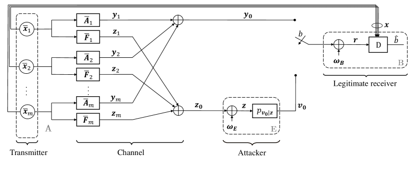
Figure 1: Anti-spoofing authentication model.

A growing number of location based services rely on global navigation satellite systems (GNSSs) for positioning and timing, but the widespread adoption of GNSSs has also increased the incentive to mount attacks against them [1]. In particular, the spoofing attack refers to the transmission of counterfeit GNSS-like signals with the intent to produce a wrong position computation at the receiver [2, 1, 3]. One of the simplest spoofing techniques is meaconing, i.e., the re-transmission of the signal received by the spoofer towards the victim, so that the latter computes the ranging estimate based on the signals seen from the spoofer location. Advanced versions of this attack selectively forge delayed versions of the ranging signals, allowing the spoofer to induce an arbitrary position estimate at the victim. When dealing with ranging signals protected by cryptography, the secure code estimation and replay (SCER) attack [4, 5] can be used to estimate the message signature and then reconstruct the signal in real-time based on the estimation. Another replay attack type, called distance-decreasing attack [6], modifies the receiver’s position by decreasing the pseudo-range estimation, attempting to decode a received symbol before the end of its duration.

In the last decade, the GNSS community has investigated anti-spoofing techniques both operating at data level and at ranging code level. Securing the range estimation means authenticating the source and protecting the integrity of the received signal, which requires to act at the physical layer. Therefore, in this paper, we focus on physical-layer authentication, which exploits the communication medium and does not rely on a higher layer encryption.

Spreading code encryption (SCE) is the most reliable option to limit access to GNSS signals as it makes the spreading code fully unpredictable for the attacker, therefore limiting its capabilities to perform a successful signal generation attack [7]. Moreover, when using SCE, a SCER attack has limited success in estimating each spreading code chip from the noisy received signal, since the chip period is typically several orders of magnitude lower than the message symbol period [8]. Some SCE solutions are the P(Y) code for GPS and the commercial authentication service (CAS) for Galileo. CAS is currently under development, but is expected to be established by 2024: in particular, a proposal known as assisted CAS (ACAS), recently presented in [9, 10], provides a SCE method where the encryption key is derived from the unpredictable signature in the Galileo open service navigation message authentication (OS-NMA) [11, 12].

A modification of the SCE approach for civilian signals is proposed in [13], where a spreading code authentication (SCA) technique, which makes use of signal watermarking, is outlined. A similar SCA technique was also presented in [14], where short sequences of spread spectrum security codes (SSSCs) are used to modify the spreading code. This design approach has evolved in [15], and has been applied in [16, 17], where the scheme called chips-message robust authentication (CHIMERA) is introduced, aiming at jointly authenticating both the navigation data and the spreading code of GPS signals for civil usage. Another solution for the joint authentication of navigation data and spreading code chips, referred to as spreading code and navigation data based authentication proposal (SNAP), can be found in [18] and a similar approach was also proposed in [7]. Other examples of SCA techniques for open GNSS signals, each employing different methods for generating and placing the watermarked chips, were introduced in [19, 20, 21]. However, existing anti-spoofing mechanisms in the literature are designed as a particular solution without any optimality criterion and their performance is evaluated against some specific attacks, which may not represent the worst case scenario for the design mechanism.

A first unified general model for the design, description, evaluation, and comparison of SCA techniques was presented in [22], where an optimal compromise is achieved between security and the number of random bits in the watermark. However, the security is only evaluated in terms of conditional guessing probability for the watermarked code given the public one, thereby neglecting the effects of channel transmission, noise, and possible SCER attacks. On the other hand, in [23] a signal authentication method based on physical layer secrecy is presented, in which the navigation signal is transmitted along with a synchronous and orthogonal authentication signal, which is in turn encoded for secrecy and corrupted by artificial noise (AN). A general security result follows from the impossibility for a spoofer to decode the authentication signal without knowledge of the AN, which is later disclosed for verification.

However, a totally general framework for deriving a wide class of solutions, optimizing their parameters, and evaluating their security against a broad set of attacks is still lacking, to the best of our knowledge, and is the aim of the present work.

This paper makes the following contributions. First, we describe a general model to characterize the spoofing attack in GNSS, considering the presence of multiple space vehicles (SVs), a victim receiver, and an attacker. We describe the optimal attack strategy that minimizes the Kullback-Leibler (K-L) divergence between the received signal distribution in nominal and attack conditions, while still introducing the desired shifts on the satellites’ signals. Indeed, the K-L divergence gives an outer bound to the detection error tradeoff (DET) curve (determined by false alarm and missed detection probabilities), which in turn is the appropriate metric to assess the capabilities of the victim receiver in detecting the attack. Therefore, the proposed optimization procedure provides an optimal attack abstracting from the particular detection process and whose efficacy can be assessed beforehand.

For a general class of attack strategies, we derive a closed form expression for the K-L divergence, and a lower bound that only depends on the GNSS scenario and channel physical parameters, regardless of the specific detection strategy adopted by the victim. Then, framing the spoofing and its detection as an adversarial game, we prove that the set of strategies comprised of a Gaussian transmission and the optimal attack is a Nash equilibrium for the game. Moreover, we discuss the K-L divergence obtained at the equilibrium points. Lastly, we consider the case of practical modulation schemes for Alice and derive the generalized likelihood ratio test. Finally, simulation results for the attack-defense scheme are presented, considering both likelihood ratio test (LRT) and generalized likelihood ratio test (GLRT) attack detection mechanisms, to validate the analytical derivations and show that the bound on the achievable error region given by the K-L divergence is representative of the actual performance.

The rest of this paper is organized as follows. Section II presents the general GNSS spoofing model in details, together with performance metrics. In Section III the optimal attack strategy is derived, then analytical results are presented. Defense strategies at both the transmitter and the receiver are discussed in Section IV. Then, numerical results are presented in Section V, employing two transmission modulations: Gaussian signaling and finite-cardinality signaling. Lastly, Section VI draws the conclusions of the paper.

Notation

Vectors and matrices are denoted by lower and upper case boldface letters, respectively. Symbol $\mathbold{A}^{\mathrm{H}}$ denotes the complex conjugate transpose of matrix $\mathbold{A}$, while $\mathbold{A}^{\dagger}$ denotes the Moore-Penrose pseudo inverse of $\mathbold{A}$. Symbol $\mathbold{I}_{n}$, denotes the identity matrix of size $n\times n$, $|\mathbold{A}|$ and $\|\mathbold{A}\|_{F}$ stand for the determinant and the Frobenius norm of $\mathbold{A}$, respectively. Given two random variables $x$ and $y$, $p_{x}$ represents the probability density function (pdf) of $x$, $p_{x|y}$ represents the conditional pdf of $x$ given $y$, and $p_{xy}$ represents the joint pdf of $x$ and $y$. If $\mathbold{a}\in\mathbb{C}^{n}$ and $\mathbold{b}\in\mathbb{C}^{m}$ are random vectors, $\mathbold{K_{ab}}=\mathbb{E}[\mathbold{ab}^{\mathrm{H}}]$ denotes their $n\times m$ covariance matrix. Finally, $\log$ denotes the natural logarithm.

II System Model

We consider a constellation of $m$ SVs (Alice, block $\rm{A}$ in Fig. 1) transmitting signals to a receiver (Bob, block $\rm{B}$ in Fig. 1). By estimating the relative delay among signals received from the $m$ SVs and by knowing the position of the SVs, Bob estimates its position through ranging techniques [24]. A third device (Eve, block $\rm{E}$ in Fig. 1) both receives the signals from the SVs and transmits them to Bob. The aim of Bob is to authenticate the received signal, i.e., to determine whether it comes from the constellation of SVs or from Eve. In turn, Eve aims at transmitting a signal that can be confused as authentic by Bob but has different delays among SV signals, to induce a different position estimation. A reliable and asynchronous side communication channel (which cannot be used for position estimation) enables the transmission of authenticated data from Alice to Bob for the verification of the GNSS signal, while Eve cannot access it to build the attack. A possible way to implement this channel is through delayed authentication techniques [25]. In this paper, we investigate how Alice can transmit its signals (on both the main and the side channel) and how Bob can perform the verification step of the authentication procedure. Also, we study possible attack strategies by Eve.

II-A Transmission Procedure

The $i$-th SV, $i\in\{1,2,...,m\}$, broadcasts a radio signal represented by its discrete-time complex baseband equivalent vector $\bar{\mathbold{x}}_{i}\in\mathbb{C}^{n}$, with $\bar{\mathbold{x}}_{i}$ independent from $\bar{\mathbold{x}}_{j}$ if $i\neq j$. We define the transmitted word $\mathbold{x}$ as the concatenation of the signals transmitted by all SVs: $\mathbold{x}=[\bar{\mathbold{x}}_{1},\bar{\mathbold{x}}_{2},...,\bar{\mathbold{x}}_{m}]\,\in\mathbb{C}^{mn}$; word $\mathbold{x}$ is also delivered to Bob over the side channel. It is important to note that the side information provided to the receiver can also be a compressed lossless version of the transmitted word $\mathbold{x}$. Two delays are associated to each signal $\bar{\mathbold{x}}_{i}$, namely $\tau_{\mathrm{B},i}$ and $\tau_{\mathrm{E},i}$, indicating the propagation time of $\bar{\mathbold{x}}_{i}$ from the $i$-th SV to Bob and to Eve, respectively. Without loss of generality we assume $\min_{i}\{\tau_{\mathrm{B},i}\}=\min_{i}\{\tau_{\mathrm{E},i}\}=0$, so that vectors $\mathbold{\tau}_{\mathrm{B}}=[\tau_{\mathrm{B},1},\tau_{\mathrm{B},2},...,\tau_{\mathrm{B},m}]$ and $\mathbold{\tau}_{\mathrm{E}}=[\tau_{\mathrm{E},1},\tau_{\mathrm{E},2},...,\tau_{\mathrm{E},m}]$ collect the relative delays between the signals coming from the $m$ satellites. Moreover, we define $\delta_{\mathrm{B}}=\max_{i}\{\tau_{\mathrm{B},i}\}$ and $\delta_{\mathrm{E}}=\max_{i}\{\tau_{\mathrm{E},i}\}$.

Signal $\bar{\mathbold{x}}_{i}$, $i\in\{1,2,...,m\}$, is transmitted through two linear channels $\mathbold{y}_{i}=\bar{\mathbold{A}_{i}}\bar{\mathbold{x}_{i}}$ and $\mathbold{z}_{i}=\bar{\mathbold{F}_{i}}\bar{\mathbold{x}_{i}}$, providing the useful signals received by Bob and Eve, respectively. Matrices $\bar{\mathbold{A}}_{i}$ and $\bar{\mathbold{F}}_{i}$ are determined by relative delays between signals, the fading environment, fluctuations in atmospheric parameters, signal distortion, and channel gains. Moreover, $\bar{\mathbold{A}}_{i}$ and $\bar{\mathbold{F}}_{i}$ include proper padding to guarantee that each channel output vector has the same size. We denote the concatenation of matrices $\bar{\mathbold{A}}_{i}$ and $\bar{\mathbold{F}}_{i}$, for $i=1,...,m$, as $\mathbold{A}=[\bar{\mathbold{A}}_{1},\bar{\mathbold{A}}_{2},...,\bar{\mathbold{A}}_{m}]\in\mathbb{C}^{(n+\delta_{\mathrm{B}})\times(mn)}$ and $\mathbold{F}=[\bar{\mathbold{F}}_{1},\bar{\mathbold{F}}_{2},...,\bar{\mathbold{F}}_{m}]\in\mathbb{C}^{(n+\delta_{\mathrm{E}})\times(mn)}$.

In nominal conditions, Bob receives the sum of the signals coming from the $m$ satellites,

$$\mathbold{y}_{0}=\sum_{i=1}^{m}\mathbold{y}_{i}=\mathbold{Ax}\,.$$ (1)

The same holds for Eve, who obtains

$$\mathbold{z}_{0}=\sum_{i=1}^{m}\mathbold{z}_{i}=\mathbold{Fx}\,.$$ (2)

Furthermore, $\mathbold{y}_{0}$ and $\mathbold{z}_{0}$ are corrupted by additive white Gaussian noise (AWGN), represented by two circularly symmetric complex Gaussian random vectors with independent entries $\mathbold{\omega}_{\mathrm{B}}\sim\mathcal{CN}(\mathbold{0},\mathbold{K}_{\mathrm{B}})$ and $\mathbold{\omega_{\mathrm{E}}}\sim\mathcal{CN}(\mathbold{0},\mathbold{K}_{\mathrm{E}})$, where $\mathbold{K}_{\mathrm{B}}=2\sigma^{2}_{\mathrm{B}}\mathbold{I}_{n+\delta_{\mathrm{B}}}$, $\mathbold{K}_{\mathrm{E}}=2\sigma^{2}_{\mathrm{E}}\mathbold{I}_{n+\delta_{\mathrm{E}}}$, and $\sigma^{2}_{\mathrm{B}}$, $\sigma^{2}_{\mathrm{E}}$ are the variances of each component (real or imaginary) of the complex noise at Bob’s and Eve’s receiver, respectively. Then, the signals received in nominal conditions by Bob and Eve are, respectively,

$$\mathbold{y}=\mathbold{y}_{0}+\mathbold{\omega_{\mathrm{B}}}\,,\;\;\;\mathbold{z}=\mathbold{z}_{0}+\mathbold{\omega_{\mathrm{E}}}\,.$$ (3)

II-B Attack Strategy

The goal of Eve is to falsify the propagation times thus introducing the forged relative delays $\mathbold{\tau}_{\mathrm{f}}=[\tau_{\mathrm{f},1},\tau_{\mathrm{f},2},...,\tau_{\mathrm{f},m}]$ corresponding to a possibly different position than the actual receiver location. We assume that: (i) Eve does not know $\mathbold{x}$ but only knows $\mathbold{z}$, which is a noisy and reduced-size version of $\mathbold{x}$; (ii) Eve knows the joint distributions of $\mathbold{x}$, $\mathbold{y}$, and $\mathbold{z}$; (iii) Eve knows the channels matrices of links $\rm{A}\rightarrow\rm{B}$, $\rm{A}\rightarrow\rm{E}$, and $\rm{E}\rightarrow\rm{B}$, and the corresponding noise statistics. We remark that the attacker cannot process each satellite signal separately: such processing would in fact require the knowledge of each word $\bar{\mathbold{x}}_{i}$, $i=1,\ldots,m$.

We assume that Eve can directly design the vector $\mathbold{v_{0}}$ received by Bob when under attack, apart from the receiver noise. Thus, when under attack the signal received by Bob is

$$\mathbold{v}=\mathbold{v_{0}}+\mathbold{\omega_{\mathrm{B}}}\,.$$ (4)

where $\mathbold{v}$, $\mathbold{v}_{0}\in\mathbb{C}^{n+\delta_{\mathrm{f}}}$, with $\delta_{\mathrm{f}}=\max\mathbold{\tau}_{\mathbold}{f}$.

Eve’s spoofing strategy can exploit the information carried by her observations $\mathbold{z}$ and, for the sake of generality, we consider that Eve adopts a probabilistic strategy, characterized by the conditional pdf $p_{\mathbold{v_{0}}|\mathbold{z}}$. Moreover, we assume that Eve knows the statistics of the noise at Bob, so that the attack strategy can be described by the pdf $p_{\mathbold}{v|z}$. Since the observation $\mathbold{z}$ encloses all the information Eve can exploit to deceive Bob, we conclude that the forging strategy $\mathbold{v}$ is conditionally independent of the transmitted word $\mathbold{x}$, given $\mathbold{z}$.

Let the received signal by Bob be

$$\mathbold{r}=\begin{cases}\mathbold{y}&\mbox{if Bob is locked on the legitimate signal }(b=0)\\ \mathbold{v}&\mbox{if Bob is locked on the spoofing signal }(b=1)\,,\end{cases}$$ (5)

where the binary variable $b$ in (5) indicates the legitimate/attack state. We assume that Eve is able to completely cancel the signal $\mathbold{y}_{0}$ at Bob, thus considering the worst case scenario where Bob acquires and locks onto the spoofed signal $\mathbold{v}$ [26]. Therefore, Eve aims at preventing Bob from distinguishing between $\mathbold{v}$ and the legitimate $\mathbold{y}$ that would be obtained with $\mathbold{\tau}_{\mathrm{B}}=\mathbold{\tau}_{\mathrm{f}}$.

II-C Authentication Procedure

The goal of the legitimate receiver Bob is to figure out if the signal $\mathbold{r}$ he receives corresponds to the authentic signal $\mathbold{y}$, or to a signal $\mathbold{v}$ that has been forged by Eve. In making this decision, Bob can make use of his knowledge of $\mathbold{x}$, which has been disclosed by Alice through the side channel. We remark that the message transmitted through the side channel can be a lossless compressed version of $\mathbold{x}$. To detect the spoofing attack, Bob performs an authentication test, wherein, given $\mathbold{x}$ and the observation $\mathbold{r}$, Bob chooses between the two hypotheses:

$$\mathcal{H}_{0} :\mathbold{r}=\mathbold{y}\,,\mbox{ the message is from Alice},$$ (6)

$$\mathcal{H}_{1} :\mathbold{r}=\mathbold{v}\,,\mbox{ the message was forged}.$$ (7)

In Fig. 1, the correct verification is achieved when $\hat{b}=b$. The authentication procedure is summarized in block $D$, which has the received signal $\mathbold{r}$ as input and outputs the Boolean value $\hat{b}$.

It is worth noting that the model in Fig. 1 includes previous models from the literature, as particular cases. In the scheme proposed in [15, 16, 17], only one satellite has been considered, which can be cast into our model by taking $m=1$. In these solutions, a small part of the spreading code is superimposed with a secret, cryptographically generated sequence, which can be subsequently reproduced by the receivers when they become aware of the key, while navigation message data are protected by digitally signing most or all the data. So, word $\mathbold{x}$ is the signal obtained by the superposition of the signed navigation data with the signed version of the spreading code, followed by a binary phase-shift keying (BPSK) modulation. Then, with a delay with respect to $\mathbold{x}$, the key is broadcast as side information, so that the receiver is able to reconstruct $\mathbold{x}$. A similar approach can be adopted to describe Galileo OS-NMA [12, 11], possibly combined with CAS [10] or ACAS features [9]. The model in [22] can be cast into this frame by restricting $\mathbold{x}$ to be a binary watermarking sequence, and the attacker to have complete ignorance on it, thus, removing his observation $\mathbold{z}$. In the authentication scheme of [23], $\mathbold{x}$ is the superposition of the transmitted authentication message and the AN component. Then, the authentication message and the AN are transmitted to the legitimate receiver through an authenticated channel.

All the parameters presented in this Section are summarized in Table I.

TABLE I: System parameters, $i\in{1,2,...,m}$

Symbol	Definition
$m$	Number of satellites
$n$	Length of the discrete time signal $\mathbold{x}_{i}$
$\mathbold{x}_{i}$	Discrete time signal transmitted by the $i$-th SV
$\mathbold{x}$	Transmitted word
$\tau_{\mathrm{B},i}$	Propagation time of $\mathbold{x}_{i}$ from the $i$-th SV to B
$\tau_{\mathrm{E},i}$	Propagation time of $\mathbold{x}_{i}$ from the $i$-th SV to E
$\tau_{\mathrm{f},i}$	False propagation time related to $\mathbold{x}_{i}$
$\mathbold{\tau_{\mathrm{B}}}$	Vector of propagation times from A to B
$\mathbold{\tau_{\mathrm{E}}}$	Vector of propagation times from A to E
$\mathbold{\tau_{\mathrm{f}}}$	Vector of false propagation times introduced by E
$\delta_{\mathrm{B}}$	Largest propagation time of signals traveling from A to B
$\delta_{\mathrm{E}}$	Largest propagation time of signals traveling from A to E
$\delta_{\mathrm{f}}$	Largest propagation time of signals traveling from E to B
$\mathbold{A}$	A$\rightarrow$ B channel matrix
$\mathbold{F}$	A$\rightarrow$ E channel matrix
$\mathbold{\omega_{\mathrm{B}}}$	AWGN in the channel A$\rightarrow$ B and E$\rightarrow$ B
$\mathbold{\omega_{\mathrm{E}}}$	AWGN in the channel A$\rightarrow$ E
$\sigma^{2}_{\mathrm{B}}$	Noise variance per component channel A$\rightarrow$ B
$\sigma^{2}_{\mathrm{E}}$	Noise variance per component channel A$\rightarrow$ E
$\mathbold{K}_{\mathrm{B}}$	Covariance matrix of $\mathbold{\omega_{\mathrm{B}}}$
$\mathbold{K}_{\mathrm{E}}$	Covariance matrix of $\mathbold{\omega_{\mathrm{E}}}$
$\mathbold{y}$	Received signal through the AWGN channel A$\rightarrow$ B
$\mathbold{z}$	Received signal through the AWGN channel A$\rightarrow$ E
$\mathbold{v_{0}}$	Signal generated by E
$\mathbold{v}$	Received signal through the AWGN channel E$\rightarrow$ B
$\mathbold{r}$	Signal received by B
$\hat{b}$	Decision made by the receiver B
$b$	Correct value for $\hat{b}$

II-D Performance Metric

The performance of an authentication system is assessed by: a) the type-I (false alarm) error probability $p_{\mathrm{FA}}$, i.e., the probability that Bob discards a message as forged by Eve while it is coming from Alice; b) the type-II (missed detection) error probability $p_{\mathrm{MD}}$, i.e., the probability that Bob accepts a message coming from Eve as legitimate. The LRT is the optimal detection method that minimizes the false alarm probability for a fixed missed detection given $p_{\mathbold}{x}$, and $p_{\mathbold}{v|z}$ [27]. However, in general, the analytical derivation of these pdf is hardly feasible. Therefore, theoretical bounds on the achievable error probability region are useful to establish the effectiveness of practical schemes.

A first bound on the achievable error region, which is the set of achievable points in the $(p_{\mathrm{FA}},p_{\mathrm{MD}})$ plane, for a given attack strategy is given by the K-L divergence. In fact, from [28] and [29] we have

$$\mathbb{D}(p_{\hat{b}|\mathcal{H}_{1}}\|p_{\hat{b}|\mathcal{H}_{0}})\leq\mathbb{D}(p_{\mathbold{rx}|\mathcal{H}_{1}}\|p_{\mathbold{rx}|\mathcal{H}_{0}})=\mathbb{D}(p_{\mathbold{xv}}\|p_{\mathbold{xy}}).$$ (8)

In (8) we have considered the joint pdf $p_{\mathbold}{rx}$ since we suppose that, at the time of verification, the legitimate receiver knows $\mathbold{x}$, and the decision $\hat{b}$ is taken based on both inputs. Therefore, defining the function

$$h(p_{\mathrm{MD}},p_{\mathrm{FA}})\triangleq p_{\mathrm{MD}}\log\frac{p_{\mathrm{MD}}}{1-p_{\mathrm{FA}}}+(1-p_{\mathrm{MD}})\log\frac{1-p_{\mathrm{MD}}}{p_{\mathrm{FA}}}\,,$$ (9)

with $p_{\mathrm{FA}},p_{\mathrm{MD}}\in[0,1]$, and observing that $p_{\hat{b}|\mathcal{H}_{0}}(1)=p_{\mathrm{FA}}$, $p_{\hat{b}|\mathcal{H}_{0}}(0)=1-p_{\mathrm{FA}}$, $p_{\hat{b}|\mathcal{H}_{1}}(1)=1-p_{\mathrm{MD}}$ and $p_{\hat{b}|\mathcal{H}_{1}}(0)=p_{\mathrm{MD}}$, (8) can be rewritten as

$$h(p_{\mathrm{MD}},p_{\mathrm{FA}})\leq\mathbb{D}(p_{\mathbold{xv}}\|p_{\mathbold{xy}}).$$ (10)

This limits the region of achievable $(p_{\mathrm{FA}},p_{\mathrm{MD}})$ values, depending on $\mathbb{D}(p_{\mathbold{xv}}\|p_{\mathbold{xy}})$, for any decision mechanism choice. 

On one hand, the aim of the attacker Eve is to narrow the achievable region, by making the value of $\mathbb{D}(p_{\mathbold{xv}}\|p_{\mathbold{xy}})$ as small as possible, operating on the attack strategy $p_{\mathbold}{v|z}$. On the other hand, Alice aims at enlarging the achievable region, by properly choosing the distribution of the transmitted word $\mathbold{x}$ in order to increase $\mathbb{D}(p_{\mathbold{xv}}\|p_{\mathbold{xy}})$. Therefore, the defense strategy is defined by the pdf $p_{\mathbold}{x}$.

The metric $\mathbb{D}(p_{\mathbold{xv}}\|p_{\mathbold{xy}})$ can be expressed in terms of attack and defense strategies as

$$\mathbb{D}(p_{\mathbold{xv}}\|p_{\mathbold{xy}})=\iint p_{\mathbold}{x}(a)p_{\mathbold}{v|x}(b|a)\log\frac{p_{\mathbold}{v|x}(b|a)}{p_{\mathbold}{y|x}(b|a)}\mbox{d}a\,\mbox{d}b\\ =\iint p_{\mathbold}{x}(a)\int p_{\mathbold}{v|z}(b|c)p_{\mathbold}{z|x}(c|a)\,\mbox{d}c\\ \;\;\;\;\cdot\log\frac{\int p_{\mathbold}{v|z}(b|c)p_{\mathbold}{z|x}(c|a)\mbox{d}c}{p_{\mathbold}{y|x}(b|a)}\,\mbox{d}a\,\mbox{d}b\,.$$ (11)

Highlighting the contribution of attack and defense strategies, let us define

$$f(p_{\mathbold}{x},p_{\mathbold}{v|z})\triangleq\mathbb{D}(p_{\mathbold{xv}}\|p_{\mathbold{xy}})\,,$$ (12)

with fixed channels $p_{\mathbold}{y|x}$ and $p_{\mathbold}{z|x}$. So, the task that we will address in this paper from the point of view of the defense can be defined as the following maximin problem:

$$\max_{p_{\mathbold}{x}}\,\min_{p_{\mathbold{v}|\mathbold{z}}}f(p_{\mathbold}{x},p_{\mathbold}{v|z}).$$ (13)

An important difference that distinguishes attack and defense strategies is that Eve knows the value of $\mathbold{\tau_{\mathrm{E}}}$ and the victim position exactly, whereas Alice’s defense strategy must be robust and symmetrical with respect to all potential receiver and channel realizations, described by matrices $\mathbold{A}$ and $\mathbold{F}$.

In Section III we will first address the inner minimization in (13), considering the model presented in Section II and assuming that $\mathbold{x}$ is Gaussian distributed. Then, after discussing the achievable K-L divergence values, the maximization task in (13) will be finally investigated in Section IV.

III Attack Strategy

We now focus on the attack strategy optimization, i.e., from (13), we aim at deriving the conditional pdf $p_{\mathbold}{v|z}$ such that

$$p_{\mathbold{v}|\mathbold{z}}^{\star}=\operatorname*{arg\,min}_{p_{\mathbold{v}|\mathbold{z}}}f(p_{\mathbold}{x},p_{\mathbold}{v|z})\,.$$ (14)

We assume that $\mathbold{x}$ is a zero mean Gaussian random vector, so $p_{\mathbold}{x}\sim\mathcal{N}(0,\mathbold{K_{x}})$ and the optimality of this choice will be proven in Section IV-A. Under this assumption, as proved in [30], there exists an optimal attack $p_{\mathbold}{v|z}^{\star}$ minimizing the divergence in (12).

Theorem 1.

Given the zero mean, jointly Gaussian random vectors $\mathbold{x}$,$\mathbold{y}$, and $\mathbold{z}$, the optimal attack $p_{\mathbold}{v|z}^{\star}$ minimizing the divergence in (12), with fixed channels $p_{\mathbold}{y|x}$ and $p_{\mathbold}{z|x}$, under the constraint that the random vectors $\mathbold{v}$ and $\mathbold{x}$ are conditionally independent given $\mathbold{z}$, belongs to the class

$$\mathcal{C}=\left\{p_{\mathbold}{v|z}\sim\mathcal{N}(\mathbold{Gz},\,\mathbold{CC^{\mathrm{H}}}+{\mathbold{K_{\mathrm{B}}}})\right\}\,,$$ (15)

and can therefore be written as a linear transformation of $\mathbold{z}$, plus independent additive white complex Gaussian noise, i.e.,

$$\mathbold{v}=\mathbold{Gz}+\mathbold{C\omega_{\mathrm{c}}}+\mathbold{\omega_{\mathrm{B}}},$$ (16)

where $\mathbold{G}\in\mathbb{C}^{(n+\delta_{\mathrm{f}})\times(n+\delta_{\mathrm{E}})}$, $\mathbold{C}\in\mathbb{C}^{(n+\delta_{\mathrm{f}})\times(n+\delta_{\mathrm{f}})}$.

Proof.

See [30, Theorem 2]. ∎

In particular, the pdf $p_{\mathbold{v}|\mathbold{z}}^{\star}$ that solves (14) is computed by optimizing over $\mathbold{G}$ and $\mathbold{C}$, so (14) becomes

$$(\mathbold{G^{\star}},\mathbold{C^{\star}})=\operatorname*{arg\,min}_{\mathbold}{G,C}f(p_{\mathbold}{x},p_{\mathbold}{v|z})\,.$$ (17)

The variance and covariance matrices of the signals defined so far are given by

$$\mathbold{K_{xy}} =\mathbold{K_{x}A}^{\mathrm{H}}\,,$$ (18a)

$$\mathbold{K_{y}} =\mathbold{AK_{x}A}^{\mathrm{H}}+\mathbold{K_{\mathrm{B}}}\,,$$ (18b)

$$\mathbold{K_{xz}} =\mathbold{K_{x}F}^{\mathrm{H}}\,,$$ (18c)

$$\mathbold{K_{z}} =\mathbold{FK_{x}F}^{\mathrm{H}}+\mathbold{K_{\mathrm{E}}}\,,$$ (18d)

$$\mathbold{K_{xv}} =\mathbold{K_{x}F}^{\mathrm{H}}\mathbold{G}^{\mathrm{H}}\,,$$ (18e)

$$\mathbold{K_{v}} =\mathbold{GFK_{x}F}^{\mathrm{H}}\mathbold{G}^{\mathrm{H}}+\mathbold{GK_{\mathrm{E}}G}^{\mathrm{H}}+\mathbold{CC}^{\mathrm{H}}+{\mathbold{K_{\mathrm{B}}}}\,,$$ (18f)

Considering (18) and following the derivations of [30], the optimal matrices are

$$\mathbold{G^{\star}}=\mathbold{AK_{x}F}^{\mathrm{H}}(\mathbold{FK_{x}F}^{\mathrm{H}})^{\dagger}\,,\\$$ (19)

and $\mathbold{C}^{\star}\in\mathbb{C}^{(n+\delta_{\mathrm{f}})\times(n+\delta_{\mathrm{f}})}$ is the square root of the covariance matrix $\mathbold{K_{v_{0}|z}}$ of the signal $\mathbold{v}_{0}$ given $\mathbold{z}$. As outlined in [30], $\mathbold{C}^{\star}$ is obtained is obtained either with a closed form expression or through an iterative process.

III-A K-L Divergence for Attacks in $\mathcal{C}$

In this Section, we will derive an analytical expression for $f(p_{\mathbold}{x},p_{\mathbold}{v|z})$ when $p_{\mathbold}{x}$ is a generic pdf with covariance matrix $\mathbold{K_{x}}$. Under the assumption that $p_{\mathbold}{v|z}\in\mathcal{C}$, defining $\mathbold{B}\triangleq\mathbold{GF}$ and $\mathbold{\eta}\triangleq\mathbold{G\omega_{\mathrm{E}}}+\mathbold{C\omega_{\mathrm{c}}}+{\mathbold{\omega_{\mathrm{B}}}}$, $\mathbold{v}$ can be written as (see (16))

$$\mathbold{v}=\mathbold{Bx}+\mathbold{\eta}\,,$$ (20)

with

$$\mathbold{\eta}\sim\mathcal{N}(\mathbold{0},\mathbold{K_{\eta}})\;,\;\;\mathbold{K_{\eta}}=\mathbold{GK_{\mathrm{E}}G}^{\mathrm{H}}+\mathbold{CC}^{\mathrm{H}}+{\mathbold{K_{\mathrm{B}}}}\,.$$ (21)

Considering the definition of $\mathbold{v}$ given in (20), the metric $f(p_{\mathbold}{x},p_{\mathbold}{v|z})$ can be computed for a generic distribution $p_{\mathbold}{x}$ and $p_{\mathbold}{v|z}\in\mathcal{C}$ as

$$\begin{split}f(p_{\mathbold}{x}&,p_{\mathbold}{v|z})=\,\mathbb{E}\left[\log\frac{p_{\mathbold{xv}}(\mathbold{x,v})}{p_{\mathbold{xy}}(\mathbold{x,v})}\right]=\mathbb{E}\left[\log\frac{p_{\mathbold{v|x}}(\mathbold{v|x})}{p_{\mathbold{y|x}}(\mathbold{v|x})}\right]\\ =&\,\mathbb{E}\left[\log\frac{p_{\mathbold{\eta}}(\mathbold{v-Bx})}{p_{\mathbold{\omega_{\mathrm{B}}}}(\mathbold{v-Ax})}\right]=\,\mathbb{E}\left[\log\frac{p_{\mathbold{\eta}}(\mathbold{\eta})}{p_{\mathbold{\omega_{\mathrm{B}}}}(\mathbold{\eta}-\mathbold{(A-B)x})}\right]\\ =&\,\mathbb{E}\left[\log\frac{p_{\mathbold{\eta}}(\mathbold{\eta})}{p_{\mathbold{\omega_{\mathrm{B}}}}(\mathbold{\eta})}\right]+\,\mathbb{E}\left[\log\frac{p_{\mathbold{\omega_{\mathrm{B}}}}(\mathbold{\eta})}{p_{\mathbold{\omega_{\mathrm{B}}}}(\mathbold{\eta-(A-B)x})}\right]\\ =&\,\mathbb{D}(p_{\mathbold}{\eta}\|p_{\mathbold}{{\omega_{\mathrm{B}}}})+\mathbb{E}\left[((\mathbold{A-B})x)^{\mathrm{H}}\mathbold{K_{\mathrm{B}}}^{-1}(\mathbold{A-B})x\right]\\ =&\,\frac{1}{2}\log\frac{|\mathbold{K_{\mathrm{B}}}|}{|\mathbold{K_{\eta}}|}+\frac{1}{2}\operatorname{tr}(\mathbold{K_{\eta}K_{\mathrm{B}}}^{-1})-\frac{(n+\delta_{\mathrm{f}})}{2}\\ &+\frac{1}{2}\left[\operatorname{tr}\left((\mathbold{B-A})\mathbold{K_{x}}(\mathbold{B-A})^{\mathrm{H}}\mathbold{K_{\mathrm{B}}}^{-1}\right)\right]\\ =&\,\frac{1}{2}\left[\sum_{i=1}^{n+\delta_{\mathrm{f}}}\left(\frac{\lambda_{i}}{\sigma^{2}_{\mathrm{B}}}-\log\left(\frac{\lambda_{i}}{\sigma^{2}_{\mathrm{B}}}\right)\right)-(n+\delta_{\mathrm{f}})\right]\\ &+\frac{1}{2\sigma^{2}_{\mathrm{B}}}\operatorname{tr}\left((\mathbold{B-A})\mathbold{K_{x}}(\mathbold{B-A})^{\mathrm{H}}\right)\,,\end{split}$$ (22)

where $\lambda_{i}$, $i\in\{1,2,...,n+\delta_{\mathrm{f}}\}$, are the eigenvalues of $\mathbold{K_{\eta}}$. We remark that (22) holds for any distribution $p_{\mathbold}{x}$, as long as the attack pdf $p_{\mathbold}{v|z}$ is taken from $\mathcal{C}$.

For convenience, we analyze the two terms of (22) separately

$$t_{1} =\frac{1}{2}\left[\sum_{i=1}^{n+\delta_{\mathrm{f}}}\left(\frac{\lambda_{i}}{\sigma^{2}_{\mathrm{B}}}-\log\left(\frac{\lambda_{i}}{\sigma^{2}_{\mathrm{B}}}\right)\right)-(n+\delta_{\mathrm{f}})\right],$$ (23)

$$t_{2} =\frac{1}{2\sigma^{2}_{\mathrm{B}}}\operatorname{tr}\left((\mathbold{B-A})\mathbold{K_{x}}(\mathbold{B-A})^{\mathrm{H}}\right)\,.$$ (24)

Since $c-1\geq\log c,\;\forall c\in\mathbb{R}^{+}$, we can state that each term of the sum in $t_{1}$ is non-negative. Moreover, $t_{1}=0$ if and only if $\lambda_{i}/\sigma^{2}_{\mathrm{B}}=1,\;\forall i\in\{1,2,...,n+\delta_{\mathrm{f}}\}$, i.e., if and only if the attacker manages to construct $\mathbold{K_{\eta}}=\mathbold{K_{\mathrm{B}}}$. On the other hand, the term $t_{2}$ in (22) is independent of the attacker noise $\mathbold{\omega_{\mathrm{E}}}$, because it does not depend on $\mathbold{K_{\eta}}$, while it depends on the covariance matrix $\mathbold{K_{x}}$, the legitimate receiver noise power $\sigma^{2}_{\mathrm{B}}$ in the nominal case, and the difference $\mathbold{A}-\mathbold{B}$, where $\mathbold{A}$ and $\mathbold{B}$ are the authentic and the forged channel matrix, respectively. Therefore, the following inequality holds

$$f(p_{\mathbold}{x},p_{\mathbold}{v|z})\geq t_{2}\,,\,\;\forall p_{\mathbold}{v|z}\in\mathcal{C}\,.$$ (25)

III-B K-L Divergence Under Optimal Attack

From (22) and (25), we observe that, for a generic $p_{\mathbold}{x}$ with covariance matrix $\mathbold{K_{x}}$, once the values of $\mathbold{A}$, $\mathbold{K_{x}}$, and $\sigma^{2}_{\mathrm{B}}$ are fixed, the lower bound for the K-L divergence can be expressed as a function of $\mathbold{B}$ as

$$\mathbb{D}_{min}(\mathbold{B})\triangleq\frac{1}{2\sigma^{2}_{\mathrm{B}}}\operatorname{tr}\left((\mathbold{B-A})\mathbold{K_{x}}(\mathbold{B-A})^{\mathrm{H}}\right)\,.$$ (26)

In particular. when the attacker succeeds in constructing $\mathbold{K_{\eta}}=\mathbold{K_{\mathrm{B}}}$, then $t_{1}=0$, and

$$f(p_{\mathbold}{x},p_{\mathbold}{v|z}^{\star})=\mathbb{D}_{min}(\mathbold{B}^{\star})\,.$$ (27)

A worth noting consideration is that, for a fixed $\mathbold{K_{x}}$, $p_{\mathbold{v}|\mathbold{z}}^{\star}$ achieves the minimum K-L divergence among all the possible attack strategies $p_{\mathbold}{v|z}\in\mathcal{C}$, regardless of the shape of $p_{\mathbold}{x}$, thus

$$f(p_{\mathbold}{x},p_{\mathbold}{v|z})\geq f(p_{\mathbold}{x},p_{\mathbold}{v|z}^{\star})\,,\;\;\forall\;p_{\mathbold{v}|\mathbold{z}}\in\mathcal{C}.$$ (28)

In particular, when $\mathbold{K_{x}}=M_{x}\mathbold{I}_{mn}$ (as further discussed in Section IV-A), $\mathbb{D}_{min}(\mathbold{B})$ can be written as

$$\mathbb{D}_{min}(\mathbold{B})=\frac{M_{x}}{2\sigma^{2}_{\mathrm{B}}}\;\|\mathbold{A}-\mathbold{B}\|_{F}^{2}\,=\,\frac{mn}{2}\,k\,\Lambda_{\mathrm{AB}}\,,$$ (29)

where

$$k=\frac{\|\mathbold{A}-\mathbold{B}\|_{F}^{2}}{\|\mathbold{A}\|^{2}_{F}}$$ (30)

represents a diversity index between $\mathbold{A}$ and $\mathbold{B}$, and

$$\Lambda_{\mathrm{AB}}=\frac{M_{x}}{\sigma^{2}_{\mathrm{B}}}\,\frac{\|\mathbold{A}\|^{2}_{F}}{mn}\,,$$ (31)

represents the average received signal to noise ratio (SNR) at Bob. It is worth noting that the attacker can always choose $\mathbold{G}$ in such a way that $k\leq 1$ (trivially setting $\mathbold{G}=0$ we have $k=1$). Moreover, in (31), the term

$$\frac{\|\mathbold{A}\|_{F}^{2}}{mn}=\frac{1}{m}\sum^{m}_{i=1}\frac{1}{n}\|\mathbold{A}\|_{F}^{2}$$ (32)

represents the average energy of the $m$ impulsive responses of the legitimate channels. Therefore, (29) describes $\mathbb{D}_{min}(\mathbold{B})$ in terms of the total length of the $m$ transmitted signals ($mn$), a measure of the difference between the channel matrices ($k$), where $\mathbold{A}$ is the matrix of the legitimate channel and $\mathbold{B}$ is the matrix of the forged channel, the SNR of the legitimate channel $A\rightarrow B$ ($\Lambda_{\mathrm{AB}}$).

III-C Limiting Scenarios

We now discuss some limiting scenarios, in which the considered spoofing attack achieves complete indistinguishability from the legitimate signal and hence cannot be detected:

S1:

$\mathbold{A}=\mathbold{F}$, that is the case wherein Eve performs a meaconing attack, inducing her own position onto Bob;

S2:

$m=1$, so both Eve and Bob receive the signal from only one satellite, and there is not sufficient diversity;

S3:

the channel $\rm{A}\rightarrow\rm{B}$ is stochastically degraded with respect to the channel $\rm{A}\rightarrow\rm{E}$.

In the following analysis, we assume that the attacker Eve makes use of the optimal attacking strategy ${p_{\mathbold{v|z}}^{\star}}$.

In scenario S1, where $\mathbold{A}=\mathbold{F}$, we have that $\delta_{\mathrm{E}}=\delta_{\mathrm{B}}=\delta_{\mathrm{f}}=\delta$. From (19), Eve gets $\mathbold{G}^{\star}=\mathbold{I_{n+\delta}}$ so that $\mathbold{B}^{\star}=\mathbold{G^{\star}F}=\mathbold{F}$, and $\mathbold{B}^{\star}=\mathbold{F}=\mathbold{A}$, which implies $\mathbb{D}_{min}(\mathbold{B}^{\star})=0$. Thus, the meaconing attack cannot be detected in this model.

In scenario S2 we are supposing $m=1$. This implies that $\delta_{\mathrm{E}}=\delta_{\mathrm{B}}=\delta_{\mathrm{f}}=0$, so $\mathbold{A}$ and $\mathbold{F}$ are left invertible. Therefore, when $\mathbold{G^{\star}}$ is computed as in (19), Eve will get $\mathbold{B^{\star}}=\mathbold{G^{\star}F}=\mathbold{A}$, which implies $\mathbb{D}_{min}(\mathbold{B}^{\star})=0$. Therefore, to have $\mathbb{D}_{min}(\mathbold{B^{\star}})>0$, Bob has to combine signals from $m>1$ satellites. However, this is also a necessary condition for the GNSS receiver to calculate the position, velocity, and time (PVT) solution.

In scenario S3 we have that the channel $\rm{A}\rightarrow\rm{B}$, represented by the conditional pdf $p_{\mathbold}{y|x}$, can be decomposed as the cascade of $p_{\mathbold}{z|x}$ and some properly chosen $p_{\mathbold}{y|z^{\prime}}$. Therefore, in this case Eve can choose $p_{\mathbold}{v|z}=p_{\mathbold}{y|z^{\prime}}$ to obtain $p_{\mathbold}{y|x}=p_{\mathbold}{v|x}$. Moreover, we have $\mathbold{y}=\mathbold{G^{\prime}z^{\prime}}+\mathbold{C^{\prime}\omega_{\mathrm{c}}}$, and Eve chooses $\mathbold{G^{\star}}=\mathbold{G^{\prime}}$ and $\mathbold{C^{\star}}=\mathbold{C^{\prime}}$, so that $\mathbold{B^{\star}}=\mathbold{A}$ and $\mathbb{D}_{min}(\mathbold{B}^{\star})=0$. Therefore, in this case, the attack goes undetected.

The more general, and more realistic, spoofing scenario occurs when $m>1$, $\mathbold{A}\neq\mathbold{F}$ and $\sigma_{\mathrm{E}}^{2}>0$. Moreover, the hypothesis in scenario S3 is very pessimistic. Therefore, in a realistic scenario, with the additional assumption that $\ker(A)\nsubseteq\ker(F)$, it is always assured that $\mathbb{D}_{min}(\mathbold{B})>0$.

IV Defense Strategy Design

The transmission and the attack detection strategies together determine the defense strategy. Therefore, in this Section, we investigate how Alice designs the transmitted signal and how Bob performs the verification step of the authentication procedure.

IV-A Gaussian Transmission

The optimal transmission strategy $p_{\mathbold}{x}^{\star}$, is given by the maximin solution of (13). We start by identifying the optimal distribution for a constrained covariance matrix, introducing the following theorem.

Theorem 2.

Given a covariance matrix $\mathbold{K_{x}}$, let us define $p_{\mathbold}{x}^{\star}\sim\mathcal{N}(0,\mathbold{K_{x}})$. If the transmission distribution $p_{\mathbold}{x}$ is to be chosen among all those with zero mean and covariance $\mathbold{K_{x}}$, the pair of strategies $(p_{\mathbold}{x}^{\star},p_{\mathbold}{v|z}^{\star})$ constitutes a saddle point of the function $f(p_{\mathbold}{x},p_{\mathbold}{v|z})$.

Proof.

For any attack strategy $p_{\mathbold}{v|z}\in\mathcal{C}$, we can compute $f(p_{\mathbold}{x},p_{\mathbold}{v|z})$ for a generic distribution $p_{\mathbold}{x}$ from (22). We note that, when $p_{\mathbold}{v|z}\in\mathcal{C}$, the K-L divergence depends on $p_{\mathbold{x}}$ only through the covariance matrix $\mathbold{K_{x}}$. Consequently, if $p_{\mathbold}{v|z}\in\mathcal{C}$, once matrices $\mathbold{A}$, $\mathbold{B}$, and $\mathbold{K_{x}}$ are set, then $f(p_{\mathbold}{x},p_{\mathbold}{v|z})$ is constant for each probability distribution $p_{\mathbold}{x}$ chosen by Alice. Therefore, we conclude that the set of strategies ($p_{\mathbold}{x}^{\star},p_{\mathbold}{v|z}^{\star}$) constitutes a saddle point for $f(p_{\mathbold}{x},p_{\mathbold}{v|z})$, since neither the attacker nor the defender can gain by an unilateral change of strategy if the strategy of the other remains unchanged. In particular

$$f(p_{\mathbold}{x},p_{\mathbold}{v|z}^{\star}) =f(p_{\mathbold}{x}^{\star},p_{\mathbold}{v|z}^{\star})\,,\,\;\forall\,p_{\mathbold}{x}\,,$$ (33)

$$f(p_{\mathbold}{x}^{\star},p_{\mathbold}{v|z}) >f(p_{\mathbold}{x}^{\star},p_{\mathbold}{v|z}^{\star})\,,\,\;\forall\,p_{\mathbold}{v|z}\,,$$ (34)

where (33) follows from (22), when the covariance matrix $\mathbold{K_{x}}$ is fixed, while (34) holds for the optimality of $p_{\mathbold}{v|z}^{\star}$ when the transmission distribution is $p_{\mathbold}{x}^{\star}$, as stated in Theorem 1. ∎

The maximin problem in (13) can be seen as a zero-sum game with two players, where $p_{\mathbold}{x}$ and $p_{\mathbold}{v|z}$ are mixed strategies, while $f(p_{\mathbold}{x},p_{\mathbold}{v|z})$ and $-f(p_{\mathbold}{x},p_{\mathbold}{v|z})$ are the average payoffs for the defender and the attacker, respectively. In this case, the set of strategies ($p_{\mathbold}{x}^{\star},p_{\mathbold}{v|z}^{\star}$), constitutes one Nash equilibrium of the game. We remark that there may be many Nash equilibria, however, for the properties of zero-sum games, they all have the same average payoff [31].

From Theorem 2, we conclude that the optimal defense strategy $p_{\mathbold}{x}^{\star}$ solving (13) must be a zero mean Gaussian distribution. Furthermore, Alice can choose the covariance matrix $\mathbold{K_{x}}$ of $p_{\mathbold}{x}^{\star}$ so that $f(p_{\mathbold}{x}^{\star},p_{\mathbold}{v|z}^{\star})$ is maximized while ensuring the constraint on the transmitted power $M_{x}$: $\operatorname{tr}(\mathbold{K_{x}})\leq mn\,M_{x}$. Given the symmetry of the problem and the transmitter’s lack of knowledge of the channel and, consequently, of the matrices $\mathbold{A}$ and $\mathbold{F}$, a reasonable choice for $\mathbold{K_{x}}$ is $\mathbold{K_{x}}=M_{x}\,\mathbold{I}_{mn}$.

From the theory of binary hypothesis testing, we know that if both the statistics of the legitimate and spoofed signal are known (i.e., if the victim is aware of the particular attack strategy adopted by the spoofer) the test yielding the minimum $p_{\mathrm{MD}}$ for any given constraint on $p_{\mathrm{FA}}$, is the LRT, also known as Neyman-Pearson criterion [27, 28]. Under the assumption that the attack strategy belongs to class $\mathcal{C}$, the detection problem reduces to the test

$$L^{\prime}=(\mathbold{r}-\mathbold{Ax})^{\mathrm{H}}\mathbold{K_{\mathrm{B}}}^{-1}(\mathbold{r}-\mathbold{Ax})\\ -(\mathbold{r}-\mathbold{Bx})^{\mathrm{H}}\mathbold{K_{\eta}}^{-1}(\mathbold{r}-\mathbold{Bx})\underset{H_{0}}{\overset{H_{1}}{\gtrless}}\theta\,.$$ (35)

When both Eve and Alice play the Nash equilibrium strategies derived in Sections III and IV-A, Bob will use the LRT since it is aware of the attack strategy distribution.

IV-B Transmission Strategies With Practical Modulation Schemes

In Section IV-A we derived that the optimal defense strategy solving (13) must be a zero mean Gaussian distribution. However, in practice this is not feasible and hence we analyze the case wherein $\mathbold{x}$ has symbols from a finite-set, e.g., a QAM constellation.

In (22) we showed that, when $p_{\mathbold}{v|z}\in\mathcal{C}$, the value of $f(p_{\mathbold}{x},p_{\mathbold}{v|z})$ depends on $p_{\mathbold{x}}$ only through the covariance matrix $\mathbold{K_{x}}$. This implies that

$$f(p_{\mathbold}{x},p_{\mathbold}{v|z})=f(p_{\mathbold}{x}^{\star},p_{\mathbold}{v|z})\,,\;\;\forall\;p_{\mathbold}{v|z}\in\mathcal{C}\,,$$ (36)

where $p_{\mathbold}{x}$ is a generic distribution of the signal $\mathbold{x}$, with the same covariance matrix $\mathbold{K_{x}}$ of $p_{\mathbold}{x}^{\star}\sim\mathcal{N}(\mathbold{0,K_{x}})$. Therefore, when the attack belongs to the class $\mathcal{C}$, we may conclude that the performance in terms of divergence is the same with either Gaussian or finite-cardinality modulation. Moreover, from (33) and (34) we have

$$f(p_{\mathbold}{x},p_{\mathbold}{v|z}^{\star})=f(p_{\mathbold}{x}^{\star},p_{\mathbold}{v|z}^{\star})\leq f(p_{\mathbold}{x}^{\star},p_{\mathbold}{v|z})\,,\;\;\forall\;p_{\mathbold}{v|z}\,.$$ (37)

On the other hand, $p_{\mathbold}{v|z}^{\star}$ is the optimal attack strategy only when the transmitted signal $\mathbold{x}$ is a Gaussian codeword of length $mn$. This implies that, for a non Gaussian $p_{\mathbold}{x}$, an attack strategy $p_{\mathbold}{v|z}^{o}\notin\mathcal{C}$ may exist, that achieves

$$f(p_{\mathbold}{x},p_{\mathbold}{v|z}^{o})\leq f(p_{\mathbold}{x},p_{\mathbold}{v|z}^{\star})\,.$$ (38)

Therefore, from (36)–(38) we can derive the following relation

$$f(p_{\mathbold}{x},p_{\mathbold}{v|z}^{o})\leq f(p_{\mathbold}{x},p_{\mathbold}{v|z}^{\star})\\ =f(p_{\mathbold}{x}^{\star},p_{\mathbold}{v|z}^{\star})\leq f(p_{\mathbold}{x}^{\star},p_{\mathbold}{v|z}^{o})\,.$$ (39)

When the signal $\mathbold{x}$ has symbols from a finite set, the transmission strategy differs from $p_{\mathbold}{x}^{\star}$, and the optimal attack strategy distribution $p_{\mathbold}{v|z}^{o}$ is not known. Hence, the receiver only knows the statistics of the authentic signal, and cannot make assumptions on the attack strategy chosen by $\rm{E}$ nor has information on the channels $\rm{A}\rightarrow\rm{E}$ and $\rm{E}\rightarrow\rm{B}$. In this case, the LRT detection method no longer applies, and a possible solution is to use the GLRT [27, 32], i.e., the detection problem is given by

$$G^{\prime}=(\mathbold{r}-\mathbold{Ax})^{\mathrm{H}}\mathbold{K_{\mathrm{B}}}^{-1}(\mathbold{r}-\mathbold{Ax})\underset{H_{0}}{\overset{H_{1}}{\gtrless}}\theta\,.$$ (40)

V Numerical Results

In this Section we will illustrate the performance obtained for both LRT and GLRT, when either Gaussian or finite-cardinality signaling are used, under the following scenario:

• channel matrices $\mathbold{A}$ and $\mathbold{F}$ take into account only the delays, that is the propagation times of each signal $\bar{\mathbold{x}}_{i}$ from the $i$-th SV to Eve and Bob, therefore we neglect other possible channel phenomena;

• the attack strategy $p_{\mathbold}{v|z}^{\star}$ is that described in Section III.

Moreover, in a typical GNSS spoofing scenario, the power of the spoofing signal $\mathbold{v_{0}}$ at the receiver is typically larger than that of the legitimate signal; thus, the SNR on the attack signal will be significantly larger than with the authentic one. Assuming that an automatic gain control (AGC) at Bob’s front-end can scale the received signal to nearly constant amplitude, the receiver noise variance will be correspondingly reduced, in the attack case, allowing the spoofer some margin to shape $\mathbold{K_{\eta}}=\mathbold{K_{\mathrm{B}}}$. Similarly to (31), we define the received spoofer SNR as

$$\Lambda_{\mathrm{AE}}=\frac{M_{x}}{\sigma^{2}_{\mathrm{E}}}\,\frac{\|\mathbold{F}\|^{2}_{F}}{mn}\,,$$ (41)

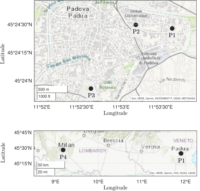
Figure 2: Map of the considered positions. Three are located in Padua, Italy: DEI (P1), Paolotti street (P2), and square of Prato della Valle (P3). One located in Milan, Italy: Duomo square (P4).

TABLE II: Considered positions and their coordinates

	LLH coordinates	Landmark
P1	$45.4077^{\circ}$ N, $11.8941^{\circ}$ E, 12 m	DEI, Padua, Italy
P2	$45.4079^{\circ}$ N, $11.8860^{\circ}$ E, 12 m	via Paolotti, Padua, Italy
P3	$45.3980^{\circ}$ N, $11.8766^{\circ}$ E, 12 m	Prato della Valle, Padua, Italy
P4	$45.4641^{\circ}$ N, $9.1903^{\circ}$ E, 120 m	Duomo square, Milan, Italy

TABLE III: Distances between Eve and target position

Eve position	Target position	Distance
P1	P2	607  m
P1	P3	1.7   Km
P1	P4	211 Km

In the analyzed scenarios, we will take into account the delay vector $\mathbold{\tau_{\mathrm{f}}}$ associated with the position of our department (DEI) (P1), located in Padua, Italy, and the delay vector $\mathbold{\tau_{\mathrm{E}}}$ associated to three different positions, two of which located in Padua, Italy, namely a house in Paolotti street (P2), and the square of Prato della Valle (P3), and the Duomo square (P4), located in Milan, Italy. Figure 2 illustrates the four positions. Delays’ measurements have been collected the 14th December 2022, at 12.00 AM. Table II outlines each considered position with their coordinates, while Table III summarizes the distances between target and Eve’s positions.

V-A Gaussian Signaling

In this Section performance is evaluated when the transmitted signal $\mathbold{x}$ is a Gaussian codeword of length $n$, considering a LRT detection method.

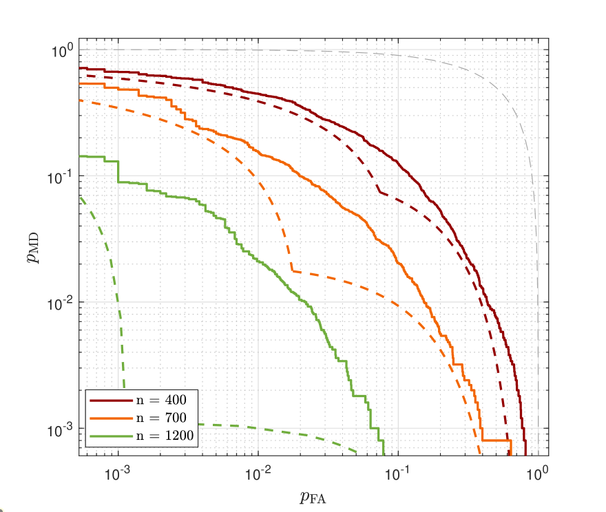
Figure 3: DET curves for the LRT detection method (solid lines) and K-L divergence bounds (dashed lines) for different values of $n$, when $p_{\mathbold}{x}$ is Gaussian distributed, $M_{x}=1$, $m=5$, $\mathbold{\tau_{\mathrm{f}}}$ associated to P1, $\mathbold{\tau_{\mathrm{E}}}$ associated to P2, $\Lambda_{\mathrm{AB}}=-25$ dB, and $\Lambda_{\mathrm{AE}}=-10$ dB. The gray dashed line represents the trivial limit case in which the decision is taken tossing a biased coin.

Fig. 3 shows the DET curves for the LRT detection method (solid lines) and the performance bounds (dashed lines) derived from the K-L divergence for different values of $n$, considering the signals coming from $m=5$ SVs, $M_{x}=1$, $\Lambda_{\mathrm{AB}}=-25$ dB, $\Lambda_{\mathrm{AE}}=-10$ dB, when $\mathbold{\tau_{\mathrm{E}}}$ and $\mathbold{\tau_{\mathrm{f}}}$ collect the delays associated to P1 and P2, respectively. The bound follows the same trend of (29), thus it is representative of the actual performance. The bound is tight for $n=400$, while the gap between it and the actual performance grows as the value of $n$ rises. Indeed, as $n$ decreases, the DET curves move quickly towards the gray dashed line, which represents the trivial limit case, in which the decision is taken without looking at the signal but tossing a biased coin. Thus, the obtained value of $p_{\mathrm{MD}}$ for given values of $p_{\mathrm{FA}}$ can be reduced by increasing the value of $n$, as Fig. 3 shows. When $n=1200$, the value of $p_{\mathrm{MD}}$ decreases by approximately one order of magnitude with respect to the case with $n=400$. Moreover, we note that the bounds given by the K-L divergence are symmetric, as proven in Appendix A.

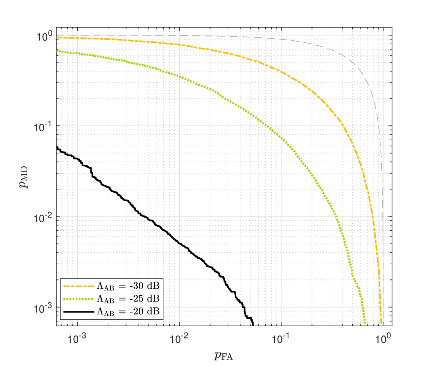
(a)

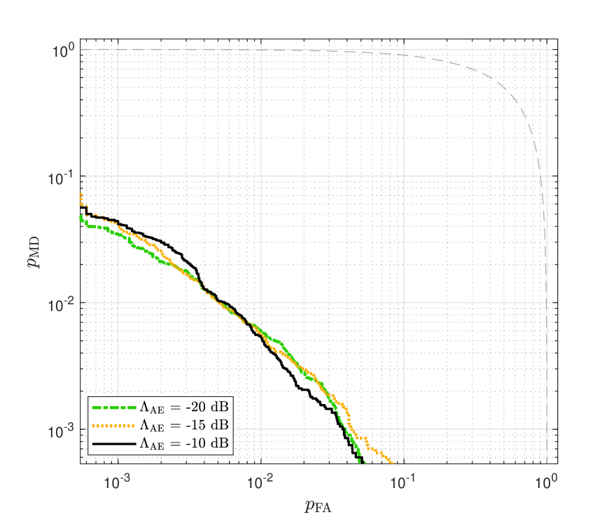
(b)

Figure 4: DET curves for the LRT detection method for different values of (a) $\Lambda_{\mathrm{AB}}$ and (b) $\Lambda_{\mathrm{AE}}$, when $p_{\mathbold}{x}$ is Gaussian distributed, $M_{x}=1$, $m=5$, $n=500$, $\mathbold{\tau_{\mathrm{f}}}$ associated to P1, and $\mathbold{\tau_{\mathrm{E}}}$ associated to P2. In (a) $\Lambda_{\mathrm{AE}}=-10$ dB, and (b) $\Lambda_{\mathrm{AB}}=-20$ dB.

Fig. 4 shows the DET curves of the LRT detection method for different values of (a) $\Lambda_{\mathrm{AB}}$ and (b) $\Lambda_{\mathrm{AE}}$, considering the signals coming from $m=5$ SVs, $M_{x}=1$, in (a) $\Lambda_{\mathrm{AE}}=-10$ dB, in (b) $\Lambda_{\mathrm{AB}}=-20$ dB, when $\mathbold{\tau_{\mathrm{E}}}$ and $\mathbold{\tau_{\mathrm{f}}}$ collect the delays associated to P1 and P2, respectively. It can be seen that the curves follow the behavior of (29); in fact, the curves rise when $\Lambda_{\mathrm{AB}}$ decreases, while remaining unchanged for different values of $\Lambda_{\mathrm{AE}}$. As a result, the performance of the LRT verification mechanism is independent of the attacker’s SNR, as long as $\Lambda_{\mathrm{AE}}>\Lambda_{\mathrm{AB}}$.

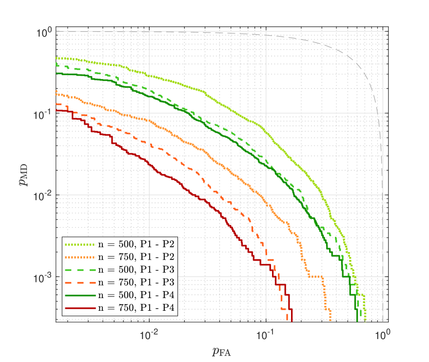
Figure 5: DET curves for the LRT detection method for different values of $n$ and position pairs, when $p_{\mathbold}{x}$ is Gaussian distributed, $M_{x}=1$, $m=5$, $\Lambda_{\mathrm{AB}}=-25$ dB, and $\Lambda_{\mathrm{AE}}=-10$ dB.

Fig. 5 shows the DET curves for the LRT detection method for different values of $n$ and position pairs, illustrated in Fig. 2, when $M_{x}=1$, $m=5$, $\Lambda_{\mathrm{AB}}=-25$ dB, and $\Lambda_{\mathrm{AE}}=-10$ dB. In each tested scenario, the delays vector $\mathbold{\tau_{\mathrm{f}}}$ is associated to P1, while the vector $\mathbold{\tau_{\mathrm{E}}}$ is associated with three different positions, i.e., (from the closest to P1 to furthest): P2, P3, and P4. We can see that the curves move away from perfect distinguishability (the lower left corner) when the distance between the position associated with $\mathbold{\tau_{\mathrm{E}}}$ and $\mathbold{\tau_{\mathrm{f}}}$ decreases. Therefore, the attack performance degrades as the attack’s target position moves farther away from the attacker’s actual position. Finally, we note that, as for Fig. 3, the defense performance improves (i.e., the curves move towards the bottom left corner) as $n$ increases.

V-B Practical Modulation Schemes

As discussed in Section IV-B, switching from Gaussian signaling to finite-cardinality signaling does not affect the performance of the verification mechanism, when the attack strategy belongs to $\mathcal{C}$. This behavior will be demonstrated in this paragraph through simulation results. In the following, a BPSK modulation will be considered (i.e., having cardinality $M=2$).

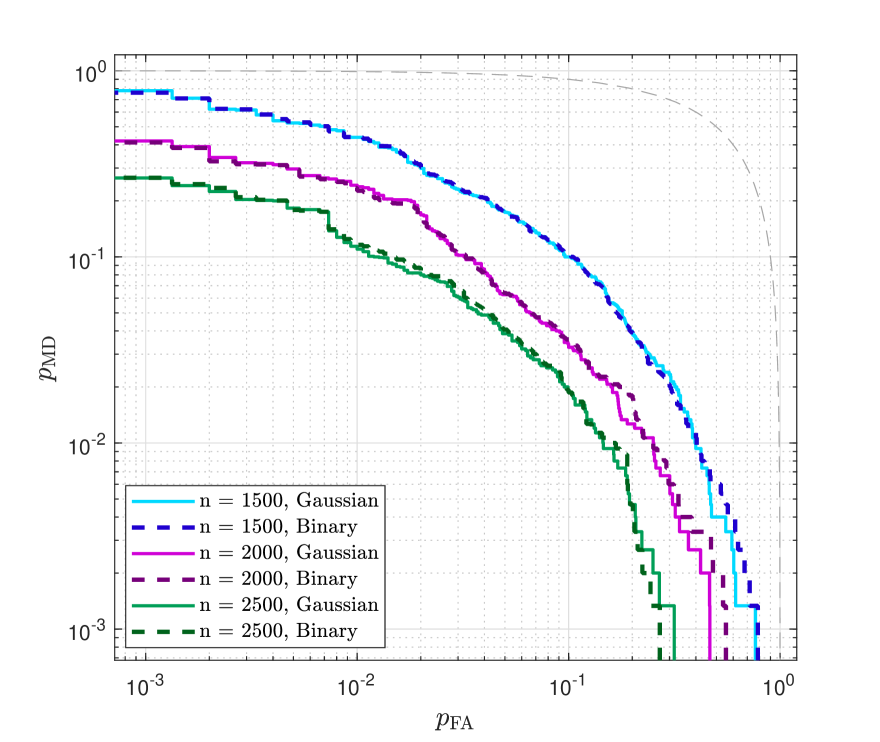
Figure 6: DET curves for the GLRT detection method for different values of $n$, when $p_{\mathbold}{x}$ is Gaussian distributed (solid lines) and when $p_{\mathbold}{x}$ is a Binary distribution (dashed lines), $M_{x}=1$, $m=9$, $\mathbold{\tau_{\mathrm{f}}}$ associated to P1, $\mathbold{\tau_{\mathrm{E}}}$ associated to P4, $\Lambda_{\mathrm{AB}}=-20$ dB, and $\Lambda_{\mathrm{AE}}=-10$ dB.

Fig. 6 shows the DET curves for the GLRT detection method for different values of $n$, when $p_{\mathbold}{x}$ is Gaussian distributed (solid lines) and $p_{\mathbold}{x}$ is a Binary distribution (dashed lines), $M_{x}=1$, $m=9$, $\mathbold{\tau_{\mathrm{f}}}$ and $\mathbold{\tau_{\mathrm{E}}}$ collect the delays associated to P1 and P4, respectively. These results have been obtained for $\Lambda_{\mathrm{AB}}=-20$ dB and $\Lambda_{\mathrm{AE}}=-10$ dB, so we are in the low-SNR regime. As can be seen, the curves obtained with Gaussian and binary signaling are very close, confirming the results of Section IV-B. Moreover, it is seen that GLRT is effective in detecting spoofing, even without any prior knowledge of the spoofer strategy. For practically meaningful values for $p_{\mathrm{FA}}$ and $p_{\mathrm{MD}}$, we should consider longer signals, so a higher value of $n$ with respect to the LRT case. Clearly, by observing more samples before taking a decision, the decision will be more accurate, but this requires to buffer and process more data. Furthermore, this leads to a longer time to authenticate (TTA). Thus, the observation period must be chosen as a trade-off between the computational resources of the device, the desired TTA, and the desired performance in terms of DET.

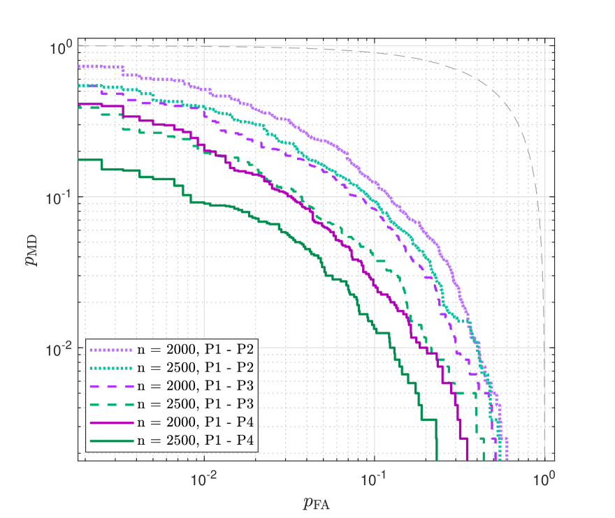
Figure 7: DET curves for the GLRT detection method for different values of $n$ and position pairs, when $p_{\mathbold}{x}$ is Gaussian distributed, $M_{x}=1$, $m=9$, $\Lambda_{\mathrm{AB}}=-20$ dB, and $\Lambda_{\mathrm{AE}}=-10$ dB.

Fig. 7 shows the DET curves for the GLRT detection method for different values of $n$ and position pairs, when $p_{\mathbold}{x}$ is Gaussian distributed, $M_{x}=1$, $m=9$, $\Lambda_{\mathrm{AB}}=-20$ dB, and $\Lambda_{\mathrm{AE}}=-10$ dB. In each tested scenario, the delay vector $\mathbold{\tau_{\mathrm{f}}}$ is associated to P1, while vector $\mathbold{\tau_{\mathrm{E}}}$ is associated with P2, P3, and P4. As for the LRT case, the attack performance improves when the distance between the position associated with $\mathbold{\tau_{\mathrm{E}}}$ and $\mathbold{\tau_{\mathrm{f}}}$ decreases. Therefore, also for the GLRT, the missed detection probability decreases, for a fixed false alarm probability, as the attack’s target position moves farther away from the attacker’s actual position.

VI Conclusion

In this paper we have proposed a general model to characterize the spoofing detection problem in GNSSs when the spoofer can observe the legitimate signal, abstracting from the specific modulation formats and cryptographic mechanisms. We have shown that effective detection can be achieved by relying only on the combination of signals from multiple SVs and on the diversity between the attacker position and the intended forged position. We have also investigated a class of attack strategies based on the statistics of the transmitted and received signals, which are shown to be optimal to minimize the K-L divergence metric. The optimal attack strategy turned out to be a proper linear transformation of the signal received at the attacker position, combined with an appropriately tuned independent additive white Gaussian noise. We have derived a lower bound on the K-L divergence, which depends only on the total length of the transmitted signals, on the SNR of the legitimate channel, and on the difference between the forged and the legitimate channel matrices. Moreover, we have discussed the results obtained in relation to different modulation schemes; we have shown that when the attack strategy is the optimal one, with Gaussian or finite-cardinality signaling we get the same performance in terms of K-L divergence. Then, we found a Nash equilibrium of the attack-defense scheme deriving the optimal defense strategy against the above-mentioned attack, which, in turn, is described by a Gaussian distribution. Finally, the performance of the detection schemes against the proposed attack has been analyzed through numerical simulations considering two verification mechanisms: LRT and GLRT.

Appendix A Symmetry of the K-L divergence

In this Appendix we provide a proof of the symmetry of the K-L divergence when the attacker uses the optimal attack strategy $p_{\mathbold}{v|z}^{\star}$, presented in Section III, and $\mathbold{K_{\eta}}=\mathbold{K_{\mathrm{B}}}$, that is

$$\mathbb{D}(p_{\mathbold{xv}^{\star}}\|p_{\mathbold{xy}})=\mathbb{D}(p_{\mathbold{xy}}\|p_{\mathbold{xv}^{\star}})\,.$$ (42)

For any $p_{\mathbold}{v|z}\in\mathcal{C}$, $\mathbb{D}(p_{\mathbold{xy}}\|p_{\mathbold{xv}})$ can be computed following the same procedure as in (22), therefore we get

$$\begin{split}\mathbb{D}&(p_{\mathbold{xy}}\|p_{\mathbold{xv}})=\frac{1}{2}\bigg{[}\log\frac{|\mathbold{K_{\eta}}|}{|\mathbold{K_{\mathrm{B}}}|}+\operatorname{tr}(\mathbold{K_{\mathrm{B}}K_{\eta}}^{-1})\\ &+\operatorname{tr}\bigg{(}(\mathbold{A-B})\mathbold{K_{x}}(\mathbold{A-B})^{\mathrm{H}}\mathbold{K_{\mathrm{B}}}^{-1}\bigg{)}-(n+\delta_{\mathrm{f}})\bigg{]}\\ =&\,\frac{1}{2}\left[\sum_{i=1}^{n+\delta_{\mathrm{f}}}\left(\frac{\sigma^{2}_{\mathrm{B}}}{\lambda_{i}}-\log\left(\frac{\sigma^{2}_{\mathrm{B}}}{\lambda_{i}}\right)\right)-(n+\delta_{\mathrm{f}})\right]\\ &+\frac{1}{2\sigma^{2}_{\mathrm{B}}}\operatorname{tr}\left((\mathbold{A-B})\mathbold{K_{x}}(\mathbold{A-B})^{\mathrm{H}}\right)\end{split}$$ (43)

When the attack strategy is $p_{\mathbold}{v|z}^{\star}$ and $\mathbold{K_{\eta}}=\mathbold{K_{\mathrm{B}}}$, we have that $\lambda_{i}=\sigma^{2}_{\mathrm{B}},\forall i\in\{1,2,...,n+\delta_{\mathrm{f}}\}$. Therefore, we obtain

$$\mathbb{D}(p_{\mathbold{xy}}\|p_{\mathbold{xv^{\star}}})=\frac{1}{2\sigma^{2}_{\mathrm{B}}}\operatorname{tr}\left((\mathbold{A-B^{\star}})\mathbold{K_{x}}(\mathbold{A-B^{\star}})^{\mathrm{H}}\right)\\ =\mathbb{D}_{min}(\mathbold{B}^{\star})=\mathbb{D}(p_{\mathbold{xv^{\star}}}\|p_{\mathbold{xy}})\,.$$ (44)

References

- [1] Z. Wu, Y. Zhang, Y. Yang, C. Liang, and R. Liu, “Spoofing and anti-spoofing technologies of global navigation satellite system: A survey,” IEEE Access, vol. 8, pp. 165 444–165 496, Sept. 2020.
- [2] D. Margaria, B. Motella, M. Anghileri, J. Floch, I. Fernandez-Hernandez, and M. Paonni, “Signal structure-based authentication for civil GNSSs: Recent solutions and perspectives,” IEEE Signal Processing Magazine, vol. 34, no. 5, pp. 27–37, 2017.
- [3] M. L. Psiaki and T. E. Humphreys, “GNSS spoofing and detection,” in Proceedings of the IEEE, vol. 104, no. 6, 2016, pp. 1258–1270.
- [4] T. E. Humphreys, “Detection strategy for cryptographic GNSS anti-spoofing,” IEEE Transactions on Aerospace and Electronic Systems, vol. 49, no. 2, pp. 1073–1090, Apr. 2013.
- [5] G. Caparra, N. Laurenti, R. Ioannides, and C. Massimo, “Improving Secure Code Estimate-Replay attacks and their detection on GNSS signals,” in Proceedings of ESA Workshop on Satellite Navigation Technologies and European Workshop on GNSS Signals and Signal Processing (NAVITEC), 2014.
- [6] K. Zhang and P. Papadimitratos, “On the effects of distance-decreasing attacks on cryptographically protected GNSS signals,” in Proceedings of the International Technical Meeting of The Institute of Navigation, 2019, p. 363–372.
- [7] J. T. Curran and M. Paonni, “Securing GNSS: An end-to-end feasibility analysis for the Galileo open-service,” in Proceedings of the 27th International Technical Meeting of the Satellite Division of The Institute of Navigation (ION GNSS+ 2014), Tampa, Florida, USA, 2014, pp. 2828–2842.
- [8] G. Caparra and J. T. Curran, “On the achievable equivalent security of GNSS ranging code encryption,” in Proceedings of IEEE/ION Position, Location and Navigation Symposium (PLANS), 2018, pp. 956–966.
- [9] R. Terris-Gallego, I. Fernandez-Hernandez, J. A. López-Salcedo, and G. Seco-Granados, “Guidelines for Galileo assisted commercial authentication service implementation,” in Proceedings of the International Conference on Localization and GNSS (ICL-GNSS), 2022, pp. 01–07.
- [10] I. Fernandez-Hernandez, S. Cancela, R. Terris-Gallego, G. Seco-Granados, J. A. López-Salcedo, C. O’Driscoll, J. Winkel, A. d. Chiara, C. Sarto, V. Rijmen, D. Blonski, and J. de Blas, “Semi-assisted signal authentication based on Galileo ACAS,” arXiv, June 2022.
- [11] I. Fernández-Hernández, V. Rijmen, G. Seco-Granados, J. Simon, I. Rodríguez, and J. D. Calle, “A navigation message authentication proposal for the Galileo open service,” NAVIGATION: Journal of the Institute of Navigation, vol. 63, no. 1, pp. 85–102, Mar. 2016.
- [12] I. F. Hernández, T. Ashur, V. Rijmen, C. Sarto, S. Cancela, and D. Calle, “Toward an operational navigation message authentication service: Proposal and justification of additional OSNMA protocol features,” in Proceedings of European Navigation Conference (ENC), 2019, pp. 1–6.
- [13] M. G. Kuhn, “An asymmetric security mechanism for navigation signals,” Information Hiding, pp. 239–252, 2005.
- [14] L. Scott, “Anti-spoofing & authenticated signal architectures for civil navigation systems,” in Proceedings of the Institute of Navigation GPS/GNSS Conference, 2003, p. 1543–1552.
- [15] ——, “Proving location using GPS location signatures: Why it is needed and a way to do it,” in Proceedings of the 26th International Technical Meeting of the Satellite Division of The Institute of Navigation (ION GNSS+ 2013), Nashville, TN, USA, 2013, pp. 2880–2892.
- [16] A. G. T. I. Air Force Research Laboratory, Space Vehicles Directorate, Chips Message Robust Authentication (CHIMERA) Enhancement for the L1C Signal : Space Segment/User Segment Interface. Interface specification IS-AGT-100, April 2019.
- [17] J. M. Anderson, K. L. Carroll, N. P. DeVilbiss, J. T. Gillis, J. C. Hinks, J. J. O’Hanlon, Brady W.and Rushanan, L. Scott, and R. A. Yazdi, “Chips-message robust authentication (CHIMERA) for GPS civilian signals,” in Proceedings of the 30th International Technical Meeting of the Satellite Division of The Institute of Navigation (ION GNSS+ 2017), September 2017, pp. 2388–2416.
- [18] B. Motella, D. Margaria, and M. Paonni, “An authentication concept for the Galileo open service,” in Proceedings of IEEE/ION Position, Location and Navigation Symposium (PLANS), 2018, pp. 967–977.
- [19] S. Wang, H. Liu, Z. Tang, and B. Ye, “Binary phase hopping based spreading code authentication technique,” Satellite Navigation, vol. 2, no. 4, Feb. 2021.
- [20] O. Pozzobon, L. Canzian, M. Danieletto, and A. D. Chiara, “Anti-spoofing and open GNSS signal authentication with signal authentication sequences,” in Proceedings of ESA Workshop on Satellite Navigation Technologies and European Workshop on GNSS Signals and Signal Processing (NAVITEC), 2010, pp. 1–6.
- [21] O. Pozzobon, G. Gamba, M. Canale, and S. Fantinato, “Supersonic GNSS authentication codes,” in Proceedings of the 27th International Technical Meeting of the Satellite Division of The Institute of Navigation (ION GNSS+ 2014), Tampa, Florida, USA, 2014, pp. 2862–2869.
- [22] N. Laurenti and A. Poltronieri, “Optimal compromise among security, availability and resources in the design of sequences for GNSS spreading code authentication,” in Proceedings of International Conference on Localization and GNSS (ICL-GNSS), 2020, pp. 1–6.
- [23] F. Formaggio and S. Tomasin, “Authentication of satellite navigation signals by wiretap coding and artificial noise,” EURASIP Journal on Wireless Communications and Networking, no. 98, Apr. 2019.
- [24] E. D. Kaplan and C. J. Hegarty, Understanding GPS, Principles and Applications - Second edition. Artech House, 2005.
- [25] I. Fernández-Hernández, T. Ashur, and V. Rijmen, “Analysis and recommendations for MAC and key lengths in delayed disclosure GNSS authentication protocols,” IEEE Transactions on Aerospace and Electronic Systems, vol. 57, no. 3, pp. 1827–1839, 2021.
- [26] T. E. Humphreys, B. M. Ledvina, M. L. Psiaki, B. W. O’Hanlon, and P. M. Kintner Jr, “Assessing the spoofing threat,” GPS World, vol. 20, no. 1, pp. 28–38, 2009.
- [27] S. M. Kay, Fundamentals of Statistical Signal Processing - Volume 2: Detection Theory. USA: Prentice-Hall, Inc., 1993.
- [28] U. M. Maurer, “Authentication theory and hypothesis testing,” IEEE Transactions on Information Theory, vol. 46, no. 4, p. 1350–1356, July 2000.
- [29] C. Cachin, “An information-theoretic model for steganography,” Proceeding of the 2nd International Workshop Information Hiding (IH), vol. LNCS-1525, pp. 306–318, 1998.
- [30] A. Ferrante, N. Laurenti, C. Masiero, M. Pavon, and S. Tomasin, “On the error region for channel estimation-based physical layer authentication over Rayleigh fading,” IEEE Transactions on Information Forensics and Security, vol. 10, no. 5, pp. 941–952, May 2015.
- [31] J. Von Neumann and O. Morgenstern, Theory of Games and Economic Behavior, 2nd rev. Princeton university press, 1947.
- [32] O. Zeitouni, J. Ziv, and N. Merhav, “When is the generalized likelihood ratio test optimal?” IEEE Transactions on Information Theory, vol. 38, no. 5, pp. 1597–1602, Sept. 1992.