Trade-off between predictive performance and FDR control for high-dimensional Gaussian model selection

Abstract

In the context of the high-dimensional Gaussian linear regression for ordered variables, we study the variable selection procedure via the minimization of the penalized least-squares criterion. We focus on model selection where the penalty function depends on an unknown multiplicative constant commonly calibrated for prediction. We propose a new proper calibration of this hyperparameter to simultaneously control predictive risk and false discovery rate. We obtain non-asymptotic theoretical bounds on the False Discovery Rate with respect to the hyperparameter and we provide an algorithm to calibrate it. It is based on completely observable quantities in view of applications. Our algorithm is validated by an extensive simulation study and is compared with some existing variable selection procedures. Finally, we propose a study to generalize our approach in complete variable selection.

Keywords Ordered variable selection  $\cdot$ Prediction  $\cdot$ FDR  $\cdot$ High-dimension  $\cdot$ Gaussian regression  $\cdot$ Hyperparameter calibration

1 Introduction.

1.1 The issue.

We consider the following high-dimensional univariate Gaussian linear regression model:

$$Y=X\beta^{*}+\varepsilon.$$ (1.1)

The random response vector $Y=\Big{(}(Y_{i})_{\{1\leq i\leq n\}}\Big{)}^{T}\in\mathbb{R}^{n}$ is regressed on $p$ deterministic vectors: $X_{1}=\Big{(}(x_{i1})_{\{1\leq i\leq n\}}\Big{)}^{T},\cdots,X_{p}=\Big{(}(x_{ip})_{\{1\leq i\leq n\}}\Big{)}^{T}$. The design matrix of size $n\times p$ is denoted by $X=\left(X_{1},\cdots,X_{p}\right)$. The noise $\varepsilon=\Big{(}(\varepsilon_{i})_{\{1\leq i\leq n\}}\Big{)}^{T}$ is assumed to be Gaussian: $\varepsilon\sim\mathcal{N}(0,\sigma^{2}I_{n})$ with $\sigma^{2}>0$. In the high-dimensional context, additional assumptions of regularity are required and we assume that $\beta^{*}$ is sparse, meaning that only a few coefficients are non-zero. In the following, a variable $X_{j}$ corresponding to a non-zero coefficient $\beta^{*}_{j}$ is called an active variable. Otherwise the variable is said to be non active.
In this paper, we are interested in variable selection. We refer the reader to [1] and references therein. To the best of our knowledge, some variable selection procedures focus on the prediction of the response variable $Y$ through a control of the predictive risk. Others focus on limiting the number of selected non active variables through a control of the False Discovery Rate. There also exists procedures where several cost functions are considered simultaneously. In the line of the latter, our goal is to identify a set of variables from a model selection procedure by limiting the selection of non active variables while maintaining accurately prediction performances.

1.2 Related works.

In a variable selection procedure, a cost function has to be defined. The predictive risk (PR) and the False Discovery Rate (FDR) are the common used cost functions.

The penalized methods to control the predictive risk.

The penalization procedure balances goodness of fit and sparsity: the smaller the penalty function, the better the fitting to the data but the higher the number of selected variables. In high-dimension, the most popular method is the Lasso criterion [2] where the estimator $\hat{\beta}_{\lambda}$ of $\beta^{*}$ is the solution of:

$$\hat{\beta}_{\lambda}=\underset{\beta\in\mathbb{R}^{p}}{\arg\min}\Big{\{}||Y-X\beta||_{2}^{2}+\lambda|\beta|_{1}\Big{\}},$$ (1.2)

where $|\cdot|_{1}$ and $||\cdot||_{2}$ design the $\ell_{1}$-norm and the euclidean norm of a vector respectively. The main challenge is to calibrate the hyperparameter $\lambda>0$. If $\lambda$ is chosen to be proportional to $\sigma\sqrt{\frac{\log(p)}{n}}$, then the predictive risk is bounded [3, 4]. However, the noise being usually unknown, the choice of $\lambda$ remains tricky. Therefore, an alternative is to solve the Lasso criterion for a $\lambda$ within a reasonable interval by using subsamples [5] or resamples [6]. The selected variables are then defined as the variables with the highest selection frequencies. Such alternative is no longer sensitive to the choice of $\lambda$ but the main challenge lies in the threshold on the frequency defining the selected variables.
In this paper, we consider a model selection procedure composed of three steps. The first step consists in solving the Lasso criterion on a relevant grid $\Lambda$. Each $\lambda\in\Lambda$ defines a variable subset to get a collection $\mathcal{M}$ of relevant subsets of variables with a wide range of sizes. In the second step, the least-squares estimator onto each variable subset of $\mathcal{M}$ is calculated leading to a collection of estimators $\left(\hat{\beta}_{m}\right)_{m\in\mathcal{M}}$. Lastly, the following penalized least-squares minimization is solved to select the best $m$ of $\mathcal{M}$:

$$\hat{m}=\underset{m\in\mathcal{M}}{\arg\min}\Big{\{}||Y-X\hat{\beta}_{m}||_{2}^{2}+\text{pen}(D_{m})\Big{\}},$$ (1.3)

where $D_{m}$ is the dimension of the model $m$ and the function pen is a penalty function increasing with $D_{m}$.
Selecting $\hat{m}$ from $\mathcal{M}$ by minimizing (1.3) corresponds to selecting $\hat{\lambda}$ from $\Lambda$ by minimizing (1.2). Hence, the main challenge is the definition of pen that makes the best trade-off between goodness of fit and sparsity within $\mathcal{M}$. Among the most famous methods for model selection, we can cite $V-$fold cross-validation [7, 8], AIC [9], Cp-Mallows [10], BIC [11] and eBIC [12]. For these penalty functions, the predictive risk is bounded when $\sigma^{2}$ is known and when the sample size $n$ tends to infinity. When $n$ is fixed, relatively small, and possibly smaller than the dimension $p$, a non-asymptotic point of view is preferable to get properties for all couples of $(n,p)$. In this direction, [13] propose some penalty functions depending on the collection complexity such that $\hat{m}$ guarantees non-asymptotic optimal control of the predictive risk. If the model collection is nested with a known variance, $\text{pen}(D_{m})=2\sigma^{2}D_{m}$ allows to achieve an optimal non-asymptotic control of the predictive risk [9]. If the model collection is fixed and large (for instance with an exponential growth with $D_{m}$) and if the variance is unknown, this optimal control is obtained with the data-driven penalties [13, 14]. Lastly, if the model collection is data-dependent and if the variance $\sigma^{2}$ is unknown, the LinSelect penalty [15, 16] guarantees an optimal control of the predictive risk.

The multiple testing methods to control the False Discovery Rate.

In the multiple testing procedure, the $p$ tests $H_{0}=\{\beta^{*}_{j}=0\}$ versus $H_{1}=\{\beta^{*}_{j}\neq 0\}$ are performed independently to get a list of $p$-values. Variables associated with a $p$-value smaller than a threshold are selected and the challenge is to find this threshold to obtain an upper bound on a function of the number of selected non active variables. First methods control the Family-Wise Error (FWER) which is the probability of selecting at least one non active variable [17, 18]. However, these methods tend to be conservative leading to a tiny set of selected variables. An alternative consists in controlling the FDR which is the expectation of the proportion of non active variables among the selected ones. The authors of [19] first provide a threshold assuming independence of the $p$-values. This hypothesis is then relaxed in [20, 21, 22, 23].
Instead of considering the $p$-values, the knockoff filter method [24] consists in introducing copies of $X_{j}$ built to be non active variables to calibrate a threshold on test statistics.

The simultaneous control of several cost functions.

Controlling PR or FDR is commonly performed independently in the literature and yield different sets of selected variables. For a PR control, selected variables aim at correctly predicting a new observation of $Y$, without guaranteeing that the set of selected variables does not contain non active variables. Conversely, when the cost function is the FDR, the number of non active variables is controlled at the price that some active variables are not selected.
Therefore, recent works have been proposed to combine prediction and FDR approaches to select all active variables without selecting non active ones. For instance, [25] propose a multi-step algorithm where a threshold procedure is applied to some Lasso estimators computed for specific values of $\lambda$. In addition to prediction performances, a consistency property on the selected variable set is satisfied under some conditions on $X$. Another idea is the post-selection inference [26, 27] where the principle is to test the relevance of each selected variable by a model selection procedure. Valid confidence intervals are provided from conditional hypothesis tests for each model of the collection in addition to a PR control. Their work has been generalized by [28, 29, 30] and a review can be found in [31].
In a completely different direction, [32, 33] propose to control the False Negative Rate (FNR) in addition to the FDR. A good FNR control ensures that most of the active variables are selected. So, minimizing a weighted sum of FDR and FNR provide a set of variables close to the set of active variables. However, improving FDR control deteriorates FNR control and vice versa. Hence, optimal controls of both criteria are impossible to achieve.
Some other papers propose to combine the FDR with the PR. Additional motivation to consider the PR is its behavior between the learning phase and the over-fitting phase. In the learning phase, the addition of a variable in the selected set drastically reduces the PR, whereas in the over-fitting phase, it increases proportionally to the noise level. Firstly, in the standard multivariate normal mean problem with a known variance, [34] propose a penalty function in the model selection procedure built from a multiple testing procedure. They obtain simultaneously sharp asymptotic bounds of the FDR and the PR. Then, [35] propose the Sorted $\ell_{1}$ penalized estimator (SLOPE) which is the minimizer of the Lasso criterion (1.2) where $\lambda$ is replaced by a $p$-vector built from a multiple testing procedure. For the orthogonal design, their approach achieves a non-asymptotic control of the FDR and satisfies a minimum value of the total mean squared error with minimax convergence rate [36]. This asymptotic convergence of the FDR has been generalized under a wide range of hypotheses, for instance, for a random design in [37].

Ordered variable selection.

The ordered variable framework has attracted much attention recently, especially to overcome the high-dimensional problem. In literature, a large class of methods exists dealing with variables having a natural ranking: [38] for the regression framework, [39] with the nested lasso penalty and [40] for covariance matrix estimation. This assumption allows for drastically reducing the estimation complexity. We develop the theory of our paper under this assumption. Time series, climatology and spatial data are typical examples where it makes sense to assume a natural order of variables and justify our model setting.
However, in most applications, no canonical ranking of the variables is available and having a natural order on variables becomes a strong assumption. In this case, alternatives consist in proposing a candidate order from random procedures and applying theoretical statistical methods on the random variable ranking. Several approaches have been implemented in the literature to provide the random orders. The most used ones are based either on a regularization path which is built with the Lasso type equation solving [2] or on a decision tree [41]. However, these approaches suffer from instability in that a small modification of the initial sample could radically change the variable order [42]. To circumvent this instability problem, one solution is to add a sampling procedure like the bootstrap [43]. We adopt this point of view in this article to generalize our theoretical results in complete variable selection.

1.3 Main contributions.

The originality of this paper is to obtain a control of the FDR in addition to the PR control in model selection through a convenient calibration of the penalty.
We assume variables are ranked according to their importance for the response variable $Y$; $X_{1}$ being the most important one, $X_{2}$ being the second one, $\cdots$, and $X_{p}$ being the least important one. In Gaussian linear regression, the order is given by the partial correlation between $Y$ and each $X_{j}$. A natural model collection is the one containing the nested models respecting the variable order. This framework sounds restrictive but allows to derive theoretical expressions of the FDR in the considered model selection procedure. According to [13], all the penalty functions defined by:

$$\text{pen}(D_{m})=K\sigma^{2}D_{m},\quad\forall m\in\mathcal{M},$$ (1.4)

provide a non-asymptotic control of the PR for $K>1$ when variables are ranked.

Theoretical bounds on the FDR in model selection: Although the model selection procedure is built for a PR control, we obtain non-asymptotic lower and upper bounds on the FDR with respect to $K>0$ when $\sigma^{2}$ is known. We show that these bounds only involve some evaluations of cumulative functions of the standard Gaussian and of some chi-squared variables. Whatever the noise level, FDR is always strictly positive. When $K$ tends to infinity, the FDR converges to $0$ with an exponential rate. So, a low value of the FDR is satisfying as soon as the value of $K$ is not too large.

Calibration of the hyperparameter $K$: The obtained theoretical bounds depend on the parameters $\beta^{*}$ and $\sigma^{2}$. We replace them with estimators to obtain completely data-dependent bounds on the FDR. Then, we propose a calibration of the hyperparameter $K$ to control a trade-off between FDR and PR. Our algorithm is validated on an extensive simulation study and is compared with some existing variable selection procedures.

Towards a complete variable selection: From a practical point of view, a crucial assumption of this work is the knowledge of the variable ranking. We provide some alternatives to apply our approach in complete variable selection. They consist in estimating the variable order to build random model collections.

1.4 Outline of the paper.

The rest of the paper is organized as follows. Section 2 introduces the Gaussian linear regression model and some notations. Section 3 contains theoretical results. Since an increase of the hyperparameter $K$ leads to a decrease of the FDR, it motivates the study of the FDR function in model selection with respect to $K$. As the FDR has an intractable expression, bounds are obtained when the variable order and the variance are known. We establish an exponential convergence rate of the FDR function when $K$ tends to infinity. The special case of orthogonal design matrix is studied to illustrate the main results. In Section 4, an algorithm is proposed to calibrate the hyperparameter $K$ in the penalty function to get a convenient trade-off between FDR and PR controls. It is based on simultaneous evaluations of the prediction performance and the FDR of the models, which are calculated from properly chosen estimators of $\sigma^{2}$ and $\beta^{*}$. We then present a study to generalize our procedure in complete variable selection and we compare our algorithm with some existing variable selection procedures. Section 5 contains conclusions and perspectives. In Section 6, proofs of all the theoretical results are provided. Lastly, validations of the chosen estimators of $\sigma^{2}$ and $\beta^{*}$, of our algorithm to calibrate $K$ and of the considered alternatives to go towards the complete variable selection are proposed in Section 7 through an extensive simulation study with different parameters.

2 Model and notations.

Let us consider the Gaussian linear regression model given in (1.1). We define $q=\min(n,p)$ and assume that $\left(X_{1},\cdots,X_{q}\right)$ is a family of linearly independent vectors. We consider the deterministic and nested model collection of linear spaces:

$$\mathcal{M}=\Big{\{}m_{0}=\{0\},m_{1}=\text{Span}(X_{1}),\cdots,m_{q}=\text{Span}(X_{1},X_{2},\cdots,X_{q})\Big{\}}.$$ (2.1)

By construction, the true model $m^{*}=\text{Span}\big{(}X_{j},\ j\ \text{s.t.}\ \beta^{*}_{j}\neq 0\big{)}$ belongs to $\mathcal{M}$.
For each $m\in\mathcal{M}$, $D_{m}$ is the dimension of $m$ and $\hat{\beta}_{m}$ is the least-squares estimator onto $m$:

$$\hat{\beta}_{m}=\underset{\{\beta,X\beta\in m\}}{\arg\min}\Big{\{}||Y-X\beta||_{2}^{2}\Big{\}}.$$

With the definition of $q$ and properties on the family $\left(X_{1},\cdots,X_{q}\right)$, $\hat{\beta}_{m}$ is unique for each $m\in\mathcal{M}$.
For all $K>0$, we define the function $\text{crit}_{K}$ on $\mathcal{M}$ as:

$$\text{crit}_{K}(m)=||Y-X\hat{\beta}_{m}||_{2}^{2}+K\sigma^{2}D_{m},$$

and the selected model $\hat{m}(K)$ by:

$$\hat{m}(K)=\underset{m\in\mathcal{M}}{\arg\min}\Big{\{}\text{crit}_{K}(m)\Big{\}}.$$ (2.2)

We define $\text{PR}(m)$ the predictive risk associated to the model $m\in\mathcal{M}$ by:

$$\text{PR}(m)=\mathbb{E}\Big{[}||Y-X\hat{\beta}_{m}||_{2}^{2}\Big{]},$$ (2.3)

where $\mathbb{E}$ designs the expectation under the distribution of $Y$ satisfying (1.1). We define successively $FP(m)$ the number of variables contained in $m$ but not in $m^{*}$, the false discovery proportion by:

$$\text{FDP}(m)=\frac{\text{FP}(m)}{\max(D_{m},1)};$$

and the False Discovery Rate by:

$$\text{FDR}(m)=\mathbb{E}\Big{[}\text{FDP}(m)\Big{]},$$

where $\mathbb{E}$ still designs the expectation under the distribution of Y satisfying (1.1), so that $\text{FDR}(m)$ is deterministic even in the case where $m$ is random.

Finally, the notation $\langle.,.\rangle$ designs the canonical scalar product in $\mathbb{R}^{n}$, $\Pi_{\mathcal{X}}$ denotes the orthogonal projection function onto the space $\mathcal{X}$, $\Phi$ designs the standard Gaussian cumulative distribution function and $F_{\chi^{2}(k)}$ is the cumulative distribution function of a chi-squared variable with $k$ degrees of freedom. By convention, an intersection or an union from indices $k$ to $\ell$ with $k>\ell$ are the intersection or the union over an empty set. In the same way, the set $\{k,\cdots,\ell\}$ is empty if $k>\ell$.

3 The main results.

In this section, the variance $\sigma^{2}$ is supposed to be known. We first present intuitions that lead to study $\text{FDR}(\hat{m}(K))$ in model selection. Non-asymptotic bounds on $\text{FDR}(\hat{m}(K))$ are obtained in Theorem 3.2, as well as asymptotic behaviors when $K$ tends to infinity in Corollary 3.4. Finally, the particular case where $X$ is the orthogonal design matrix is studied to illustrate the main results.

3.1 Intuitions.

According to [13], the penalty function (1.4) satisfies a non-asymptotic control of the PR if and only if $K>1$. The constant $K=2$ allows to achieve the optimal asymptotic control of the PR. Hence, $2$ is commonly chosen in practice but other values of $K$ close to $2$ can give equivalent even better non-asymptotic prediction performances. In this direction, we propose to calibrate the hyperparameter $K$ among those leading to prediction performances close to or better than for $K=2$ while satisfying a control of the FDR. The calibration is based on both $\text{PR}(\hat{m}(K))$ and $\text{FDR}(\hat{m}(K))$ functions with respect to $K$.

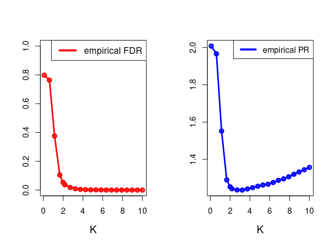
Figure 1: Curves of the empirical $\text{FDR}\big{(}\hat{m}(K)\big{)}$ and $\text{PR}\big{(}\hat{m}(K)\big{)}$ for the toy data set described in Subsection 7.1.

In Figure 1, we propose an illustration of our intuitions by plotting the empirical estimators of $\text{PR}(\hat{m}(K))$ and $\text{FDR}(\hat{m}(K))$ on a regular grid of positive $K$. Graphs are obtained from the toy data set described in Section 7. We observe that for all $K\in[2,3]$, the empirical $\text{PR}(\hat{m}(K))$ values are kept low while the $\text{FDR}(\hat{m}(K))$ function decreases with $K$. Hence, in this example, the choice $K=3$ is more judicious than $K=2$ since it ensures a stronger control of the FDR while satisfying similar prediction performances. While FDR decreases with $K$, PR increases from a certain value of $K\geq 2$. Hence, to control PR and FDR simultaneously, the constant $K$ must not be too far from $2$.
Increasing the constant $K$ to limit the non active variable selection is known for the asymptotic point of view. Indeed, AIC and Cp-Mallows penalties [9, 10], where $K$ equals $2$, give asymptotically the best set of variables for prediction performances; while BIC penalty [11], where $K$ is fixed to $\log(n)$, exactly recovers asymptotically the set of active variables. Obtaining the asymptotic properties of AIC, Cp-Mallows and BIC penalties simultaneously is impossible [44], but it suggests that a value of $K\in[2,\log(n)]$ would get reasonable (but not necessarily optimal) values for both PR and FDR in a non-asymptotic framework. In this way, we propose to study the function $\text{FDR}\big{(}\hat{m}(K)\big{)}$ in the model selection procedure (2.2) where the penalty function is (1.4) in the ordered variable setting.

3.2 Bounds on the FDR in model selection.

3.2.1 FDR expression in model selection for ordered variables.

Let us assume that $K>0$ and $\text{crit}_{K}$ is injective on $\mathcal{M}$. If $D_{m}^{*}=q$, $\text{FDR}(\hat{m}(K))=~{}0$. Otherwise, the $\text{FDR}(\hat{m}(K))$ is expressed within the model selection procedure as:

$$\text{FDR}(\hat{m}(K))=\underset{r=D_{m^{*}}+1}{\overset{q}{\sum}}\frac{r-D_{m^{*}}}{r}\mathbb{P}\left(\left\{\underset{\underset{\ell\neq r}{\ell=0}}{\overset{q}{\cap}}\{\text{crit}_{K}(m_{r})<\text{crit}_{K}(m_{\ell})\}\right\}\right).$$ (3.1)

A detailed proof of (3.1) can be found in Subsection 6.1.

By using the decomposition

$$\left\{\underset{\ell=0}{\overset{r-1}{\cap}}\{\text{crit}_{K}(m_{r})<\text{crit}_{K}(m_{\ell})\}\right\}\bigcap\left\{\underset{\ell=r+1}{\overset{q}{\cap}}\{\text{crit}_{K}(m_{r})<\text{crit}_{K}(m_{\ell})\}\right\}$$

of the term $\underset{\underset{\ell\neq r}{\ell=0}}{\overset{q}{\cap}}\{\text{crit}_{K}(m_{r})<\text{crit}_{K}(m_{\ell})\},$ we obtain the following proposition:

Proposition 3.1.

Let us consider the ordered variable framework and the model collection (2.1) where $q=\min(n,p)$, $m^{*}\in\mathcal{M}$ and $D_{m}^{*}<q$. Let us assume that $\text{crit}_{K}$ is injective on $\mathcal{M}$. We consider $\left(u_{1},\cdots,u_{n}\right)$ an orthonormal basis of $\mathbb{R}^{n}$ such that $\text{Span}(X_{1},\cdots,X_{j})=\text{Span}(u_{1},\cdots,u_{j}),\ \forall j\in\{1,\cdots,q\}$.
Then, $\forall K>0$,

$$\text{FDR}(\hat{m}(K))=\underset{r=D_{m^{*}}+1}{\overset{q}{\sum}}\frac{r-D_{m^{*}}}{r}\ P_{r}(K)\ Q_{r}(K,\beta^{*},\sigma^{2}),$$ (3.2)

where for each $r\in\{D_{m^{*}}+1,\cdots,q\}$,

$$P_{r}(K)=\mathbb{P}\bigg{(}\underset{\ell=r+1}{\overset{q}{\cap}}\Big{\{}\underset{k=r+1}{\overset{\ell}{\sum}}Z_{k}^{2}<K(\ell-r)\Big{\}}\bigg{)},$$ (3.3)

$\text{where}\ \ Z_{k}\overset{i.i.d.}{\sim}\mathcal{N}(0,1),\ \ \forall k\in\{r+1,\cdots,q\}$,

$$\text{and}\ Q_{r}(K,\beta^{*},\sigma^{2})=\mathbb{P}\bigg{(}\underset{\ell=0}{\overset{r-1}{\cap}}\Big{\{}\underset{k=\ell+1}{\overset{r}{\sum}}\langle Y,u_{k}\rangle^{2}>K\sigma^{2}(r-\ell)\Big{\}}\bigg{)}.$$

Proof of Proposition 3.1 can be found in Subsection 6.1.

3.2.2 General bounds.

In (3.2), the $P_{r}(K)$ terms do not depend on data. Conversely, the $Q_{r}(K,\beta^{*},\sigma^{2})$ terms depend on the data. Thus, to understand the behavior of the FDR function with respect to $\hat{m}(K)$, we propose to bound the $Q_{r}(K,\beta^{*},\sigma^{2})$ terms in the following theorem:

Theorem 3.2.

Let us consider the ordered variable framework and the model collection (2.1) where $q=\min(n,p)$. Let us suppose that $m^{*}\in\mathcal{M}$ and $D_{m}^{*}<q$. The notation $\Phi$ stands for the standard gaussian cumulative distribution function and $F_{\chi^{2}(k)}$ is the cumulative distribution function of a chi-squared variable with $k$ degrees of freedom. Let us assume that $\forall K>0,\text{crit}_{K}$ is injective on $\mathcal{M}$. We consider $\left(u_{1},\cdots,u_{n}\right)$ an orthonormal basis of $\mathbb{R}^{n}$ such that $\text{Span}(X_{1},\cdots,X_{j})=\text{Span}(u_{1},\cdots,u_{j}),\ \forall j\in\{1,\cdots,q\}$.
Then, $\forall K>0$, $\hat{m}(K)$ satisfies:

$$b(K,\beta^{*},\sigma^{2})\leq\text{FDR}(\hat{m}(K))\leq B(K,\beta^{*},\sigma^{2}),$$ (3.4)

where $\Big{[}K\mapsto b(K,\beta^{*},\sigma^{2})\Big{]}$ and $\Big{[}K\mapsto B(K,\beta^{*},\sigma^{2})\Big{]}$ are two real-valued functions on $\mathbb{R}^{+}$ defined by:

$$b(K,\beta^{*},\sigma^{2})=\sum\limits_{r=D_{m^{*}}+1}^{q}\Bigg{(}\frac{r-D_{m^{*}}}{r}P_{r}(K)\ \underline{f}_{r}(K,\beta^{*},\sigma^{2})\Bigg{)},$$

$$B(K,\beta^{*},\sigma^{2})=\sum\limits_{r=D_{m^{*}}+1}^{q}\Bigg{(}\frac{r-D_{m^{*}}}{r}P_{r}(K)\ \overline{f}_{r}(K,\beta^{*},\sigma^{2})\Bigg{)},$$ (3.5)

where for all $K>0$, $P_{r}(K)$ is defined in (3.3) and

1. $\text{for each}\ r\in\{D_{m^{*}}+1,\cdots,q\}\ \text{and for all}\ \ell\in\{1,\cdots,r\},\ \underline{f}_{\ell}(\cdot,\beta^{*},\sigma^{2})$  is defined by:

   $$\underline{f}_{1}(K,\beta^{*},\sigma^{2}) =G_{1}$$

   $$\underline{f}_{\ell}(K,\beta^{*},\sigma^{2}) =G_{\ell}+H_{\ell}\ \underline{f}_{\ell-1}(K,\beta^{*},\sigma^{2}),\quad\forall\ell\in\{2,\cdots,r\},$$

   $\hskip 5.69046pt\text{with for}\ \ \ell\in\{1,\cdots,D_{m^{*}}\}$:

   $$G_{\ell}=2-\bigg{(}\Phi\big{(}\sqrt{\ell K}-\frac{\langle X\beta^{*},u_{\ell}\rangle}{\sigma}\big{)}+\Phi\big{(}\sqrt{\ell K}+\frac{\langle X\beta^{*},u_{\ell}\rangle}{\sigma}\big{)}\bigg{)},$$

           for $\ell\in\{2,\cdots,D_{m^{*}}\}$:

   $$H_{\ell}=\Phi\Big{(}\sqrt{\ell K}-\frac{\langle X\beta^{*},u_{\ell}\rangle}{\sigma}\Big{)}+\Phi\Big{(}\sqrt{\ell K}+\frac{\langle X\beta^{*},u_{\ell}\rangle}{\sigma}\Big{)}$$

   $$\quad\quad\quad-\bigg{(}\Phi\Big{(}\sqrt{K}-\frac{\langle X\beta^{*},u_{\ell}\rangle}{\sigma}\Big{)}+\Phi\Big{(}\sqrt{K}+\frac{\langle X\beta^{*},u_{\ell}\rangle}{\sigma}\Big{)}\bigg{)},$$

   $\hskip 25.6073pt\text{for}\ \ \ell\in\{D_{m^{*}}+1,\cdots,r\}:$

   $$G_{\ell}=2\bigg{(}1-\Phi\big{(}\sqrt{\ell K}\big{)}\bigg{)}$$

   $$H_{\ell}=2\bigg{(}\Phi\big{(}\sqrt{\ell K}\big{)}-\Phi\big{(}\sqrt{K}\big{)}\bigg{)},$$

2. $\forall r\in\{D_{m^{*}}+1,\cdots,q\},\ \overline{f}_{r}(\cdot,\beta^{*},\sigma^{2})$ is defined by:

   $$\overline{f}_{r}(K,\beta^{*},\sigma^{2}) =1-\max\Bigg{(}\underset{\ell\in\{1,\cdots,r-D_{m^{*}}\}}{\max}\Big{(}F_{\chi^{2}(\ell)}(\ell K)\Big{)},$$

   $$\hskip 5.69046pt\underset{\ell\in\{r-D_{m^{*}}+1,\cdots,r\}}{\max}\bigg{(}F_{\chi^{2}(\ell)}\Big{(}\frac{\ell K}{2}-\underset{k=r-\ell+1}{\overset{D_{m^{*}}}{\sum}}\frac{\langle X\beta^{*},u_{k}\rangle^{2}}{\sigma^{2}}\Big{)}\bigg{)}\Bigg{)}.$$

Proof of Theorem 3.2 can be found in Subsection 6.2.
Hence, although the model selection procedure is built for prediction performances, bounds on the FDR are derived with respect to $\hat{m}(K)$. Terms $\underline{f}_{r}(K,\beta^{*},\sigma^{2})$ and $\overline{f}_{r}(K,\beta^{*},\sigma^{2})$ only involve some evaluations of cumulative distribution functions of the standard Gaussian and chi-squared variables. So, they have a fully explicit form which makes easier the understanding of the behavior of the FDR in model selection. However, they depend on the unknown parameters $\beta^{*}$ and $\sigma^{2}$ for which estimations are proposed in Section 4.1.2

3.2.3 Strictly positive FDR.

The following corollary gives a lower bound on the FDR independent from $\sigma^{2}$.

Corollary 3.3.

Under the assumptions and definitions of Theorem 3.2, $\forall K>0$:

$$\text{FDR}(\hat{m}(K))\geq\sum\limits_{r=D_{m^{*}}+1}^{q}\Bigg{(}\frac{r-D_{m^{*}}}{r}P_{r}(K)\ \frac{2\sqrt{2}}{\sqrt{\pi}\Big{(}\sqrt{rK}+\sqrt{rK+4}\Big{)}}e^{-\frac{rK}{2}}\Bigg{)}\ >0.$$

Proof of Corollary 3.3 can be found in Subsection 6.3.
From Corollary 3.3, $\text{FDR}(\hat{m}(K))>0$ for all $K>0$ and whatever $\sigma^{2}$. This may be counter-intuitive, especially in the noiseless setting. When $\sigma^{2}=0$, $Y~{}=~{}X\beta^{*}$ and the minimization in (2.2) is reduced to the least-squares criterion minimization. So, in this particular noiseless case, $\hat{\beta}_{m^{*}}=\beta^{*}$ and the associated least-squares criterion is zero. However, the probability of having a zero value of the least squares for $m\in\mathcal{M}$ such that $m^{*}\subset m$ is non-zero and for such $m$, $\text{FDP}(\hat{m})>0$ as well as $\text{FDR}(\hat{m})>0$, by taking the expectation.

3.2.4 Asymptotic analysis.

The following corollary gives the asymptotic behavior of the FDR function in model selection when $K$ tends to infinity.

Corollary 3.4.

Under the assumptions and the definitions of Theorem 3.2, the $\text{FDR}(\hat{m}(K))$ function tends to $0$ when $K$ tends to infinity and satisfies $\forall\eta>0$,

$$\text{FDR}(\hat{m}(K))=\underset{K\longrightarrow+\infty}{o}\Big{(}e^{-K(\frac{1}{2}-\eta)}\Big{)}.\\$$ (3.6)

Furthermore, $\ \forall\eta>0,\ \exists C_{\eta}>0,\ \exists L_{\eta}>0,\ \forall K>L_{\eta},$ we have:

$$\text{FDR}(\hat{m}(K))\geq C_{\eta}e^{-K\Big{(}\frac{D_{m^{*}}+1+2\eta}{2}\Big{)}}.$$ (3.7)

So, $\forall\varepsilon>0,$

$$-\frac{D_{m^{*}}}{2}-\frac{1}{2}-\varepsilon\ \leq\ \underset{K\longrightarrow+\infty}{\lim\inf}\frac{1}{K}\log\Big{(}\text{FDR}(\hat{m}(K))\Big{)}$$

$$\underset{K\longrightarrow+\infty}{\lim\sup}\frac{1}{K}\log\Big{(}\text{FDR}(\hat{m}(K))\Big{)}\ \leq\ -\frac{1}{2}+\varepsilon.$$ (3.8)

Proof of Corollary 3.4 can be found in Subsection 6.4.
From Equation (3.6), $\text{FDR}(\hat{m}(K))$ tends to $0$ when $K$ tends to $+\infty$ with at least an exponential convergence rate and Equation (3.7) suggests that the exponential convergence rate is optimal.

Remark 3.5.

With no signal ($\beta^{*}=0$ and $D_{m^{*}}=0$), the asymptotic bounds in (3.8) are $-\frac{1}{2}-\varepsilon$ and $-\frac{1}{2}+\varepsilon$ and consequently:

$$\log\Big{(}\text{FDR}(\hat{m}(K))\Big{)}\underset{K\rightarrow+\infty}{\sim}-\frac{1}{2}K.$$

Remark 3.6.

The asymptotic upper and lower bounds (3.6) and (3.7) are satisfied whatever the value of $\sigma^{2}>0$. It is possible to obtain the following sharpest asymptotic upper bound: $\ \forall\tilde{\eta}>0,$

$$\text{FDR}(\hat{m}(K))=o\bigg{(}e^{-\Big{(}K\frac{(D_{m^{*}}+1-\tilde{\eta})}{4}-\frac{1}{2\sigma^{2}}\underset{k=1}{\overset{D_{m^{*}}}{\sum}}\langle X\beta^{*},u_{k}\rangle^{2}\Big{)}}\bigg{)}$$ (3.9)

in the asymptotic regime where $K\longrightarrow+\infty$ and $\sigma\longrightarrow 0\ \text{with}\ \frac{1}{\sigma}=\underset{\sigma\longrightarrow 0}{o}(\sqrt{K})$. The reader can find the proof in Subsection 6.4.

3.3 Illustrations of the main result in the orthogonal case.

We propose to analyze the particular case where the design matrix $X$ is orthogonal since it leads to simplified forms for the FDR bounds easy to implement.

Corollary 3.7 (Application on the orthogonal case).

Under assumptions of Theorem 3.2 and by assuming that $\left(X_{1},\cdots,X_{q}\right)$ are orthonormal for $\langle.,.\rangle$, then:
$\forall K>0,\text{FDR}(\hat{m}(K))$ satisfies the same inequalities as (3.4) where:
for $\ell\in\{1,\cdots,D_{m^{*}}\}:$

$$G_{\ell}=2-\bigg{(}\Phi\Big{(}\sqrt{\ell K}-\frac{\beta^{*}_{\ell}}{\sigma}\Big{)}+\Phi\Big{(}\sqrt{\ell K}+\frac{\beta^{*}_{\ell}}{\sigma}\Big{)}\bigg{)},$$

for $\ell\in\{2,\cdots,D_{m^{*}}\}:$

$$H_{\ell}=\Phi\Big{(}\sqrt{\ell K}-\frac{\beta^{*}_{\ell}}{\sigma}\Big{)}+\Phi\Big{(}\sqrt{\ell K}+\frac{\beta^{*}_{\ell}}{\sigma}\Big{)}-\bigg{(}\Phi\Big{(}\sqrt{K}-\frac{\beta^{*}_{\ell}}{\sigma}\Big{)}+\Phi\Big{(}\sqrt{K}+\frac{\beta^{*}_{\ell}}{\sigma}\Big{)}\bigg{)},$$

for all $r\in\{D_{m^{*}}+1,\cdots,q\}:$

$$\overline{f}_{r}(K,\beta^{*},\sigma^{2})=1-\max\Bigg{(} \underset{\ell\in\{1,\cdots,r-D_{m^{*}}\}}{\max}\Big{(}F_{\chi^{2}(\ell)}(\ell K)\Big{)},$$

$$\underset{\ell\in\{r-D_{m^{*}}+1,\cdots,r\}}{\max}\bigg{(}F_{\chi^{2}(\ell)}\Big{(}\frac{\ell K}{2}-\underset{k=r-\ell+1}{\overset{D_{m^{*}}}{\sum}}\frac{\beta^{*2}_{k}}{\sigma^{2}}\Big{)}\bigg{)}\Bigg{)},$$

and all other terms are the same as those defined in Theorem 3.2.

Proof of Corollary 3.7 can be found in Subsection 6.5.

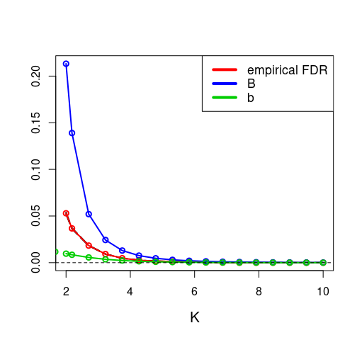
Figure 2: Left: curves of the empirical $\text{FDR}(\hat{m}(K))$ (red) and of the terms $b(K,\beta^{*},\sigma^{2})$ (green) and $B(K,\beta^{*},\sigma^{2})$ (blue) for the orthogonal design matrix $X$ for the toy data set described in Subsection 7.1. Right: curves are plotted only for $K\geq 2$.

In Figure 2, we plot the empirical estimation of the $\text{FDR}(\hat{m}(K))$ with the functions $b(K,\beta^{*},\sigma^{2})$ and $B(K,\beta^{*},\sigma^{2})$ on a grid of positive $K$ (left) and for $K\geq 2$ (right). Graphs are obtained from the toy data set described in Section 7 where $X$ is orthogonal. The left figure is devoted to illustrate Corollary 3.7. The FDR values are well smaller than the upper bound values and larger than the lower bound ones. From the right figure and in accord with Corollary 3.4, the empirical $\text{FDR}(\hat{m}(K))$ values tend to $0$ when $K$ increases and the convergence rate seems to be exponential. Moreover, the curves of $b(K,\beta^{*},\sigma^{2})$ and $B(K,\beta^{*},\sigma^{2})$ frame the empirical FDR and the difference between the three functions becomes quickly negligible for $K$ larger than $2$.

4 Trade-off between the PR and the FDR controls.

While bounds $b(K,\beta^{*},\sigma^{2})$ and $B(K,\beta^{*},\sigma^{2})$ are easily understandable and fully implementable, they depend on $\beta^{*}$, $\sigma^{2}$ and $D_{m}^{*}$, unknown in practice. For a practical use, we propose to replace the theoretical bounds on the FDR as well as the theoretical expression of the PR with observable quantities (Subsection 4.1). Then, we propose an algorithm to calibrate the hyperparameter $K$ from the data set such that both PR and FDR are controlled (Subsection 4.2).

As variables are not usually naturally ranked, we propose to test the robustness of our algorithm to variable order and we study some alternatives to generalize our method to complete variable selection. Results are provided in Subsection 4.3. Lastly, our algorithm is compared with some existing variable selection procedures in Subsection 4.4, in terms of both PR and FDR.

4.1 Estimation of the theoretical terms.

When $n$ is fixed, empirical approaches are not adapted. An alternative is to replace the theoretical terms by observable quantities.

4.1.1 Estimation of the PR.

Commonly, the predictive risk is evaluated with the mean squared error on a validation set independent from the training set used to estimate the parameters (see Formula (7.1) for the definition). However, it requires separating the dataset in two parts which increases the estimation errors. Here, we propose to use the entire dataset to both apply the model selection procedure and evaluate the predictive risk. Intuitively, the response vector $Y$ is replaced with $X\hat{\beta}_{\hat{m}(2)}$ which provides good prediction performances [13]. Moreover, by re-expressing the PR, it is straightforward to show that for all $K>0$ and $K^{{}^{\prime}}>0$:

$$\mathbb{E}[||Y-X\hat{\beta}_{\hat{m}(K)}||_{2}^{2}] -\mathbb{E}[||Y-X\hat{\beta}_{\hat{m}(K^{{}^{\prime}})}||_{2}^{2}]$$

$$=\mathbb{E}[||X\hat{\beta}_{\hat{m}(2)}-X\hat{\beta}_{\hat{m}(K)}||_{2}^{2}]-\mathbb{E}[||X\hat{\beta}_{\hat{m}(2)}-X\hat{\beta}_{\hat{m}(K^{{}^{\prime}})}||_{2}^{2}]$$

$$\hskip 28.45274pt-2\mathbb{E}[\langle X\hat{\beta}_{\hat{m}(2)}-Y,X\hat{\beta}_{\hat{m}(K^{{}^{\prime}})}-X\hat{\beta}_{\hat{m}(K)}\rangle].$$ (4.1)

According to [45], the constant $2$ provides the optimal asymptotic control of (2.3), so $||Y-X\hat{\beta}_{\hat{m}(2)}||_{2}$ is close to $0$. Moreover, $X\hat{\beta}_{\hat{m}(2)}$ is close to $\Pi_{\text{Im}(X)}(Y)$, so $X\hat{\beta}_{\hat{m}(2)}-Y$ almost belongs to the subspace $\text{Im}(X)^{\perp}$. In addition, $X\hat{\beta}_{\hat{m}(K)}$ and $X\hat{\beta}_{\hat{m}(K^{{}^{\prime}})}$ belongs to $\text{Im}(X)$, so the last term in (4.1) is close to $0$ and is negligible compared to the two others. So, for all $K>0$ and $K^{{}^{\prime}}>0$, $\mathbb{E}[||Y-X\hat{\beta}_{\hat{m}(K)}||_{2}^{2}]-\mathbb{E}[||Y-X\hat{\beta}_{\hat{m}(K^{{}^{\prime}})}||_{2}^{2}]$ equals $\mathbb{E}[||X\hat{\beta}_{\hat{m}(2)}-X\hat{\beta}_{\hat{m}(K)}||_{2}^{2}]-\mathbb{E}[||X\hat{\beta}_{\hat{m}(2)}-X\hat{\beta}_{\hat{m}(K^{{}^{\prime}})}||_{2}^{2}]$ up to an additive negligible term. Hence, the constant $K$ minimizing $\mathbb{E}[||X\hat{\beta}_{\hat{m}(2)}-X\hat{\beta}_{\hat{m}(K)}||_{2}^{2}]$ and the one minimizing $\mathbb{E}[||Y-X\hat{\beta}_{\hat{m}(K)}||_{2}^{2}]$ are almost equal. Therefore, to evaluate the prediction performances of $\hat{m}(K)$, we propose to compare prediction performances of the estimates $X\hat{\beta}_{\hat{m}(K)}$ and $X\hat{\beta}_{\hat{m}(2)}$. We introduce the following term that we call estimated difference in predictions:

$$\widehat{\text{diff-PR}}(\hat{m}(K))=\frac{1}{n}\underset{i=1}{\overset{n}{\sum}}\Big{(}\big{(}X\hat{\beta}_{\hat{m}(2)}\big{)}_{i}-\big{(}X\hat{\beta}_{\hat{m}(K)}\big{)}_{i}\Big{)}^{2}.$$ (4.2)

For the rest of the paper, the empirical version of (4.2) is calculated averaging over $100$ independent data sets and is denoted diff-PR. If this difference is significantly smaller than the noise level $\sigma^{2}$, the model $\hat{m}(K)$ has performances similar to those satisfied by $\hat{m}(2)$.

4.1.2 Estimation of the FDR.

The functions $b(\cdot,\beta^{*},\sigma^{2})$ and $B(\cdot,\beta^{*},\sigma^{2})$ are explicit and easily implementable but depend on $\beta^{*}$, $\sigma^{2}$ and $D_{m}^{*}$, which are unknown.
We propose:

1. to apply the slope heuristic method [13] to get an estimator $\hat{\sigma}^{2}$ of $\sigma^{2}$,

2. to replace $\beta^{*}$ by the estimator $\hat{\beta}_{\hat{m}(4)}$,

3. to replace $D_{m^{*}}$ by the number of non zero in $\hat{\beta}_{\hat{m}(4)}$.

Justifications are provided in Subsection 7.2.

4.2 A data-dependent calibration of $K$ in model selection procedure.

We propose a completely data-driven calibration of the hyperparameter $K$ using the functions $K\longrightarrow B(\cdot,\hat{\beta}_{\hat{m}(4)},\hat{\sigma}^{2})$ and $K\longrightarrow\widehat{\text{diff-PR}}(\hat{m}(K))$ to obtain a low value of both PR and FDR.
We propose the following algorithm:

1. Choose $\alpha$ the threshold for the FDR control and $\gamma$ the threshold for the estimated risk estimated difference in predictions (4.2).

2. Compute $I_{1}=\Big{\{}K\geq 2,\ B(K,\hat{\beta}_{\hat{m}(4)},\hat{\sigma}^{2})\ \in\ ]0,\alpha[\Big{\}}$.

3. Compute $I_{2}=\Big{\{}K\geq 2,\ \widehat{\text{diff-PR}}(\hat{m}(K))<\gamma\times\hat{\sigma}^{2}\Big{\}}$.

4. If $I_{1}\cap I_{2}\neq\emptyset$, return $\min\Big{\{}K,\ K\in I_{1}\cap I_{2}\Big{\}}$ ;

Otherwise, return $\min\Big{\{}K,K\ \in I_{1}\Big{\}}$ or take a larger value of either $\alpha$ or $\gamma$.

Algorithm 1 Algorithm to calibrate $K$

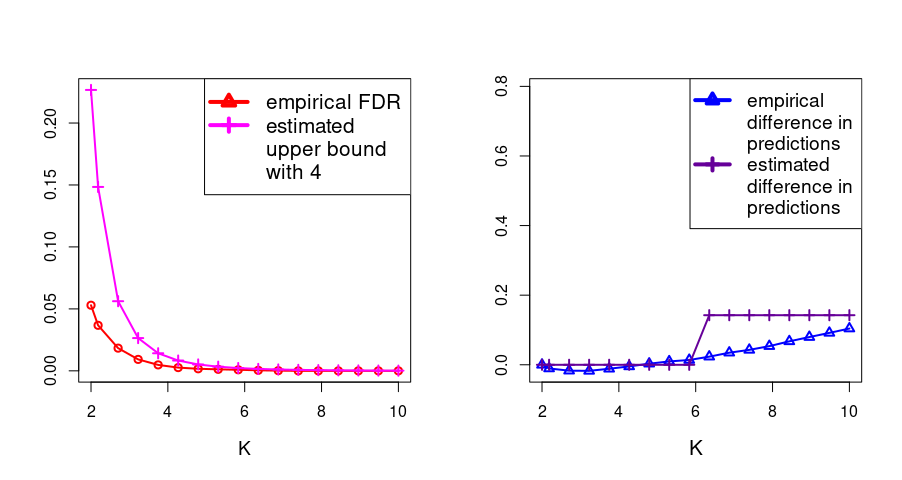
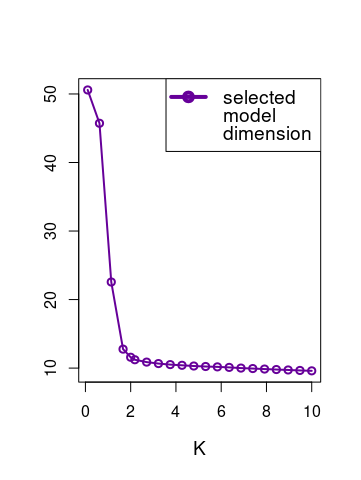
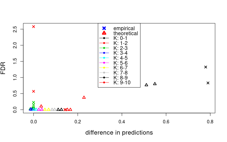
Figure 3: Top: Curves of the empirical functions $\text{FDR}\big{(}\hat{m}(K)\big{)}$ (red) and diff-PR$\big{(}\hat{m}(K)\big{)}$ (blue), of the $B(K,\hat{\beta}_{\hat{m}(4)},\hat{\sigma}^{2})$ functions (pink) and of $\widehat{\text{diff-PR}}\big{(}\hat{m}(K)\big{)}$ (violet) for $K\geq 2$ for the toy data set. Bottom: Curves of the $D_{\hat{m}(K)}$ as function of $K$ (left) and values of the empirical $\text{FDR}\big{(}\hat{m}(K)\big{)}$ and $B(K,\hat{\beta}_{\hat{m}(4)},\hat{\sigma}^{2})$ as functions of diff-PR$\big{(}\hat{m}(K)\big{)}$ and $\widehat{\text{diff-PR}}\big{(}\hat{m}(K)\big{)}$ (right) for all $K>0$ and for the toy data set.

Curves of Figure 3 are generated from the toy data set and from the simulation protocol described in Subsection 7.1. For this example, we choose $\alpha=0.05$ and $\gamma=0.1$ The interpolation of the points on the graph at bottom right of Figure 3 could be interpreted as a ROC curve parameterized by $\hat{m}(K)$. It shows that there exists some constants $K$ for which a trade-off between both theoretical FDR and PR and both empirical FDR and PR can be achieved: here for a value of $K$ between $2$ and $6$. These values correspond to a selected model dimension close to $D_{m^{*}}$ (Figure 3 at the bottom left). By applying our algorithm on this example, we get $I_{1}=[3.3,10]$ and $I_{2}=[2,5.8]$ and so, our proposed algorithm returns $K=3.3$. The evaluation of the prediction performances provided by the selected model $\hat{m}(3.3)$ is equal to $1.14$ and we get $B(3.3,\hat{\beta}_{\hat{m}(4)},\hat{\sigma}^{2})=0.03$. This constant $K=3.3$ corresponds to a low value of both empirical predictive risk and FDR functions. Indeed, the empirical predictive risk of $\hat{m}(3.3)$ is equal to $1.24$ and the empirical FDR of $\hat{m}(3.3)$ is equal to $0.01$. To compare with the usual choice $K=2$, the empirical predictive risk of $\hat{m}(2)$ is equal to $1.25$ and the empirical FDR of $\hat{m}(2)$ is equal to $0.05$. Hence, our proposed algorithm allows to maintain the prediction performances from $\hat{m}(2)$, reinforce the control of the FDR criterion and so gain a convenient trade-off between PR and FDR.

In Subsection 7.4, the algorithm 1 is applied to several data sets generated from various sets of parameters and described in Table 3. Each time, the hyperparameter $K$ is strictly larger than the commonly used constant $2$ and provides a low value of FDR while maintaining the prediction performances given by $\hat{m}(2)$.

4.3 Towards the complete variable selection

For most applications, no canonical order of variables is available and our algorithm cannot be applied directly. We propose to generate candidate orders from random procedures to use our method in complete variable selection.
More precisely, we first study the robustness to variable order of our method (Subsection 4.3.1) and provide some procedures to construct variable orders in practice (Subsection 4.3.2). Our algorithm 1 is then applied from the generated rankings in Subsection 4.4.

4.3.1 Robustness to variable order

We propose numerical experiments where the assumption of ordered variables is not fulfilled. The goal is to test the robustness to variable order of our algorithm by measuring how this impacts its performances. We consider the toy data set where the size of the true model is $D_{m^{*}}=10$ and we consider three collections which are the results of a random permutation of the nested model collection (2.1) on respectively the first ten, the first twelve and the first fifteen variables. Hence, active variables remain first in the first collection; perturbations may introduce non active variables among the first ten variables in the second collection, while in the third collection, some active variables can be pushed far into the collection.

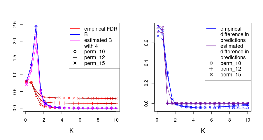
Figure 4: Curves of the empirical functions $\text{FDR}\big{(}\hat{m}(K)\big{)}$ (red) and diff-PR$\big{(}\hat{m}(K)\big{)}$ (blue), of the $B(K,\beta^{*},\sigma^{2})$ functions (blue), the $B(K,\hat{\beta}_{\hat{m}(4)},\hat{\sigma}^{2})$ functions (pink) and $\widehat{\text{diff-PR}}\big{(}\hat{m}(K)\big{)}$ (violet) for the toy data set and for the three perturbed collections.

To test the robustness to variable order of our algorithm, Figure 4 shows how the empirical FDR behaves in relation to its estimated upper bound as well as the empirical and estimated differences in predictions for the three perturbed collections. We observe that when the permutation concerns only the active variables (on the nested model collection (2.1)), values of the empirical FDR are smaller than the values of $B(K,\beta^{*},\sigma^{2})$ and $B(K,\hat{\beta}_{\hat{m}(4)},\hat{\sigma}^{2})$ which are close. For prediction, the diff-PR function has the same behavior than for the nested model collection (2.1).
When the permutation concerns the first twelve and the first fifteen variables, the empirical FDR is higher than $B(K,\beta^{*},\sigma^{2})$ and $B(K,\hat{\beta}_{\hat{m}(4)},\hat{\sigma}^{2})$ as soon as $K\geq 2$ and with an increasing deviation when the error on estimated variable order increases. Moreover, we observe that the rate of the empirical FDR decay is much slower and values are high whatever the value of $K$: above $0.13$ and $0.28$ for respectively the second and third perturbed model collection. For prediction, the diff-PR function is stable for $K\geq 2$.
Hence, permutations among only the active variables have no effect on FDR and PR. However, as soon as a non active variable is ranked before an active variable, the theoretical guarantees of Theorem 3.2 no longer hold and empirical FDR can be high whatever the value of $K$. To tackle this problem, one solution consists in combining our algorithm with a method discriminating active and non-active variables. We consider this direction for the rest of this section.

4.3.2 Random variable order

We consider four strategies to estimate variable orders. The Bolasso procedure [6] consists in solving the Lasso equation (1.2), through the LARS algorithm [46], on several resamples and for different values of $\lambda$. Variables are ranked according to their occurrence frequency in the models averaged over the $\lambda$’s and the resamples. The random forests [43] are aggregation of several binary decision trees. The tree predictors are generated on bootstrap resamples and on a subset of variables randomly chosen. Here, we combine the random forest with the recursive feature elimination (RFE) algorithm [47] whose efficiency has been proved especially for correlated variables [48]. Variables are ordered according to their importance defined by the random forest. The Sorted $\ell_{1}$ penalized estimator (SLOPE) [35] is obtained by solving the Lasso equation (1.2) with $\lambda$ a $p$-vector calculated from a multiple testing procedure. Lastly, the knockoff method [24] consists in building a non active copy $\tilde{X}_{j}$ of each $X_{j}$ and solving the Lasso equation (1.2) for several values of $\lambda$ on the augmented matrix composed on the $X_{j}$ and $\tilde{X}_{j}$ variables. Variables are then sorted according to the values of

$$W_{j}=\max\left(Z_{j},\tilde{Z}_{j}\right)\times\text{sign}\left(Z_{j}-\tilde{Z}_{j}\right),$$

where $Z_{j}$ and $\tilde{Z}_{j}$ correspond to the largest $\lambda$ for which $X_{j}$ and $\tilde{X}_{j}$ are respectively selected. For each strategy, a random model collection, on which model selection can be applied is defined from the estimated variable order. Bolasso and random forest both provide a variable order from a prediction point of view, whereas SLOPE and the knockoff method provide a variable order by considering both PR and FDR controls.

To quantify the ability to discriminate between active and non active variables, we calculate the proportion of active variables in models of size $5$, $10$, $15$ and $20$ of each random collection. Results are presented in Table 1 where each value is the average over $100$ independent iterations. With Bolasso, random forests and SLOPE, $50$ resamples for the construction of random collections are considered.

	Bolasso	SLOPE	random forests	the knockoff method
$D_{m}$ = 5	0.99	0.99	0.98	1.00
$D_{m}$ = 10	0.83	0.83	0.82	0.85
$D_{m}$ = 15	0.92	0.92	0.90	0.90
$D_{m}$ = 20	0.95	0.95	0.93	0.92

Table 1: Proportion of active variables in models of size $5$, $10$, $15$ and $20$ for random collections built with Bolasso, SLOPE, random forest and the knockoff method. Each value is the average over $100$ independent iterations.

The collection built by the knockoff method is the collection containing the fewest non active variables in the models of size $5$ and $10$. For models of size $15$ and $20$, Bolasso and SLOPE are slightly better and the proportion of active variables is always larger than $0.9$. We observe with the model of size $20$ that there are active variables far away in the collections, which is undesirable. In the following, we consider now the random collections built with the knockoff method and Bolasso (since Bolasso is slightly better than SLOPE on scenarios described in Table 3 (see Subsection 7.3)).

4.4 Comparison with other variable selection methods

Performances of Algorithm 1 are compared with three variable selection procedures. The LinSelect penalty [16] is a model selection criterion introduced in a non-asymptotic setting to take into account of the randomness of the model collection. The penalty function provides a sharp oracle inequality. The $V$-fold cross-validation [49, 50, 51] is the most popular, adaptive and simple variable selection method. The final selected model is the one with the best prediction performance accuracy over the data sets obtained by splitting the initial data set into a training set and a validation set. The last method is the knockoff method where the final variable subset is composed by $X_{j}$ such that $W_{j}\geq T$ where $T$ is defined to satisfy a given control of FDR. LinSelect and $V$-fold cross-validation aim at providing a control of PR while the knockoff method aims at providing a control of FDR.

We consider the $50$-fold cross-validation and evaluate PR and FDR of our algorithm and of the three variable selection procedures on the nested model collection (2.1) where the active variables are properly ranked before the non active variables and on random collections built with Bolasso and with the knockoff method.

	$D_{\hat{m}}$	PR($\hat{m}$)	FDR($\hat{m}$)
nested model collection
LinSelect	8.86	1.35	0.01
$50$-fold CV	26.42	2.29	0.45
Knockoff
Our algorithm	9.37	1.25	0.00
Bolasso collection
LinSelect	10.17	1.93	0.07
$50$-fold CV	22.10	2.77	0.37
Knockoff
Our algorithm	13.96	1.59	0.25
the knockoffs collection
LinSelect	8.86	1.81	0.03
$50$-fold CV	20.85	2.45	0.35
Knockoff	0.00	14.10	0.00
Our algorithm	13.33	1.65	0.18

Table 2: Results of the dimension, PR and FDR of the selected models obtained by LinSelect, the $50$-fold CV, the knockoff method and our algorithm, applied on the nested model collection (2.1) and on random collections built with Bolasso and the knockoff method. Each value is the average over $100$ independent iterations. PR and FDR of each selected model are the empirical quantities. Input parameters of our algorithm are fixed to $\gamma=0.1$ and $\alpha=0.05$. Note that the knockoff variable selection method is adapted for only the knockoff random model collection.

Table 2 shows the performances of the four variable selection procedures. As the knockoff method is a procedure for both collection generation and variable selection, the knockoff collection is only used with the knockoff variable selection method. On the nested model collection (2.1), our algorithm provides the smallest values in both FDR and PR and the average of the selected model sizes is the closest to the true model size. LinSelect behaves in a similar way while the $50$-fold cross validation selects a model located in the over-fitting area providing a high value of both PR and FDR. On random model collections, performances are deteriorated for all methods, as expected, and are slightly better on model collections built with the knockoff method than with Bolasso. Our algorithm provides the smallest PR but LinSelect provides the smallest FDR. While LinSelect is designed to control the PR theoretically, we remark that it is apparently also a relevant candidate to control FDR and to achieve a trade-off between both PR and FDR. The $50$-fold cross validation method provides poor results while the knockoff method selects the empty set of variable. The size of the model selected by our algorithm is larger when the collections are random and provides high values of FDR. These results show that a meticulous choice of $\gamma$ and $\alpha$ is important to improve our algorithm performances.

The robustness of our algorithm to variable order, the construction of random model collections and performances of the four variable selection procedures are studied on several data sets generated from various sets of parameters and described in Table 3. Results are presented in Subsection 7.3 and Subsection 7.4 and the conclusions remain the same.

5 Conclusions.

The variable selection procedure in a high-dimensional Gaussian linear regression with sparsity assumption is commonly used to identify a set of variables with prediction performances or with as few non active variables as possible. For prediction performances, the PR is usually controlled via a penalized least-squares minimization; to avoid the selection of non active variables, the FDR is usually controlled via a multiple testing approach. Controlling the PR tends to select too many variables, including non active ones, whereas controlling the FDR tends to select too few variables, leaving out some active ones.

This work shows that a convenient trade-off between PR and FDR can be achieved in ordered variable selection. The originality of this paper is to obtain this trade-off through a proper calibration of the hyperparameter $K$ in the penalty of the model selection (1.4). Firstly, theoretical results lead to non-asymptotic lower and upper bounds on the $\text{FDR}\big{(}\hat{m}(K)\big{)}$ function when $\sigma^{2}$ is known. Asymptotic behaviors suggest that bounds are optimal. Secondly, the proposed methodology provides an algorithm to calibrate the hyperparameter $K$ in the penalty function when $\sigma^{2}$ is unknown. This algorithm is based on completely data-driven terms: the estimated difference in predictions and the estimated upper bound on the FDR where the choices of estimators $\hat{\sigma}^{2}$ and $\hat{\beta}_{\hat{m}(4)}$ are derived from an extensive simulation study. The hyperparameter $K$ is calibrated from the dataset to ensure $\widehat{\text{diff-PR}}(\hat{m}(K))<\gamma\times\hat{\sigma}^{2}$ under the constraint $B(K,\hat{\beta}_{\hat{m}(4)},\hat{\sigma}^{2})<\alpha$. Our algorithm is validated on an extensive simulation study and allows to obtain a selected model ensuring a small value of both theoretical PR and FDR. The calibrated hyperparameter $K$ is strictly larger than the commonly used constant $K=2$. Moreover, PR and FDR values of the selected model with our algorithm are the smallest values compared with the existing variable selection procedures considered in the paper. Lastly, we propose a preliminary response to construct a random model collection to extend our work in complete variable selection. The performances of our algorithm deteriorate as soon as a non active variable is ranked before an active one, but combined with procedures with high ability to discriminate between active and non active variables, our algorithm is competitive with some existing variable selection procedures.

If $D_{\hat{m}(K)}=q$ for one $K>1$, the lower and upper bounds equal $0$. This means that a distinction between $D_{m^{*}}=q$ and $D_{m^{*}}<q$ is not possible without additional arguments. This is a limitation of our work.

The main perspective of our work is to generalize our theoretical results to complete variable selection. The ordered variable assumption is the key ingredient of our proofs and appears in the second line of the proof where the ratio is fixed, allowing randomness only on $\hat{m}$ that we control thanks to the ordered model selection theory. Hence, relaxing this assumption requires new technical arguments and this is a real challenge for future work. Moreover, in complete variable selection, the penalty function (1.4) has to include a logarithm term to take into account that all possible models should be explored but this is very time consuming due to the combinatorial computation explosion. In this case, two hyperparameters have to be calibrated. Another way to generalize our work in complete variable selection is to detect the value of $K$ from which the theoretical FDR is larger than the theoretical upper bound on the FDR and quantify the gap between the theoretical upper bound and the FDR.

One way to improve the performances of our algorithm can be a meticulous choice of the algorithm input parameters $\alpha$ and $\gamma$, which are arbitrarily fixed in our work.
Achieving a trade-off between FDR and PR is not trivial and investigating alternatives in this direction can be considered as perspectives. In particular, satisfying some trade-offs between PR and FDR for each model of the generated collection can be judicious in processing our variable selection then.
A possible opening is to study the potential characteristics of the hyperparameter $K$ provided by our algorithm in a theoretical point of view (dependence in $\beta^{*}$ and $\sigma^{2}$). Another possible extension is to study the false negative rate (FNR) function in the model selection procedure, similarly and in addition to the FDR one. This can provide a more powerful method, similarly to [32, 33].
Finally, another generalization is to extend our theoretical results to unknown variance, random model collections or to non-fixed designs, which are more general frameworks adapted to some application points of view. These extensions are much more intricate.

6 Proofs of theoretical results.

This section contains proofs of all the theoretical results of this paper.

6.1 FDR expression in model selection.

Proof of Formula 3.1.
If $D_{m}^{*}=q$, then $\text{FP}(m)=0$ for all $m\in\mathcal{M}$ and $\text{FDR}(m)=0$ for all $m\in\mathcal{M}$.
Let us now suppose that $D_{m}^{*}<q$. The FDP expression within the model selection procedure is:

$$\forall K>0,\quad\quad\text{FDP}(\hat{m}(K)) =\frac{\text{FP}(\hat{m}(K))}{\max(D_{\hat{m}(K)},1)}$$

$$\underset{\textit{(*)}}{=}\quad\frac{D_{\hat{m}(K)}-D_{m^{*}}}{D_{\hat{m}(K)}}\mathds{1}_{\{D_{\hat{m}(K)}>D_{m^{*}}\}}$$

$$=\underset{r=1}{\overset{q}{\sum}}\frac{r-D_{m^{*}}}{r}\mathds{1}_{\{r>D_{m^{*}}\}}\mathds{1}_{\{D_{\hat{m}(K)}=r\}}$$

$$\underset{\textit{(**)}}{=}\underset{r=D_{m^{*}}+1}{\overset{q}{\sum}}\frac{r-D_{m^{*}}}{r}\mathds{1}_{\left\{\hat{m}(K)=m_{r}\right\}}$$

$$\underset{\textit{(***)}}{=}\underset{r=D_{m^{*}}+1}{\overset{q}{\sum}}\frac{r-D_{m^{*}}}{r}\mathds{1}_{\left\{\underset{\underset{\ell\neq r}{\ell=0}}{\overset{q}{\cap}}\{\text{crit}_{K}(m_{r})<\text{crit}_{K}(m_{\ell})\}\right\}}.$$

(*) and (**) are due to the fact that models $\left(m\right)_{m\in\mathcal{M}}$ are nested and $m^{*}\in\mathcal{M}$. (***) is obtained since the $\text{crit}_{K}$ function is injective on $\mathcal{M}$. Finally, by taking the expectation, we obtain the FDR expression (3.1). ∎

Proof of Proposition 3.1.
Before proving Proposition 3.1, let us cite and prove two lemmas.

Lemma 6.1.

For $r\in\{D_{m^{*}}+1,\cdots,q\}$ and for all $\ell\in\{0,\cdots,r-1\}$:

$$||Y-X\hat{\beta}_{m_{r}}||_{2}^{2}-||Y-X\hat{\beta}_{m_{\ell}}||_{2}^{2}=-\underset{k=\ell+1}{\overset{r}{\sum}}\langle Y,u_{k}\rangle^{2}.$$

Lemma 6.2.

For $r\in\{D_{m^{*}}+1,\cdots,q\}$ and for all $\ell\in\{r+1,\cdots,q\}$:

$$||Y-X\hat{\beta}_{m_{r}}||_{2}^{2}-||Y-X\hat{\beta}_{m_{\ell}}||_{2}^{2}=\underset{k=r+1}{\overset{\ell}{\sum}}\langle Y,u_{k}\rangle^{2}.$$

Proof of Lemma 6.1.
For $r\in\{D_{m^{*}}+1,\cdots,q\}$ and $\ell\in\{0,\cdots,r-1\}$:

$$||Y-X\hat{\beta}_{m_{r}}||_{2}^{2}-||Y-X\hat{\beta}_{m_{\ell}}||_{2}^{2}=||X\hat{\beta}_{m_{r}}||_{2}^{2}-||X\hat{\beta}_{m_{\ell}}||_{2}^{2}+2\langle Y,X\hat{\beta}_{m_{\ell}}-X\hat{\beta}_{m_{r}}\rangle$$

$$=||X\hat{\beta}_{m_{r}}||_{2}^{2}-||X\hat{\beta}_{m_{\ell}}||_{2}^{2}+2\langle Y-X\hat{\beta}_{m_{r}},X\hat{\beta}_{m_{\ell}}\rangle$$

$$\hskip 85.35826pt-2\langle Y-X\hat{\beta}_{m_{r}},X\hat{\beta}_{m_{r}}\rangle+2\langle X\hat{\beta}_{m_{r}},X\hat{\beta}_{m_{\ell}}\rangle-2||X\hat{\beta}_{m_{r}}||_{2}^{2}$$

$$=-||X\hat{\beta}_{m_{r}}||_{2}^{2}-||X\hat{\beta}_{m_{\ell}}||_{2}^{2}+2\langle X\hat{\beta}_{m_{r}},X\hat{\beta}_{m_{\ell}}\rangle=-||X\hat{\beta}_{m_{r}}-X\hat{\beta}_{m_{\ell}}||_{2}^{2}.$$

The last line is due to the fact that $Y-X\hat{\beta}_{m_{r}}\in(m_{r})^{\perp}\subset(m_{\ell})^{\perp}$ since $m_{\ell}\subset m_{r}$ and $X\hat{\beta}_{m_{r}}$ is the projection of $Y$ onto $m_{r}$.
Then,

$$||X\hat{\beta}_{m_{r}}-X\hat{\beta}_{m_{\ell}}||_{2}^{2} =||\Pi_{m_{r}}(Y)-\Pi_{m_{\ell}}(Y)||_{2}^{2}$$

$$=||\Pi_{\text{Span}(X_{1},\cdots,X_{r})}(Y)-\Pi_{\text{Span}(X_{1},\cdots,X_{\ell})}(Y)||_{2}^{2}$$

$$\underset{\textit{(*)}}{=}||\Pi_{\text{Span}(u_{1},\cdots,u_{r})}(Y)-\Pi_{\text{Span}(u_{1},\cdots,u_{\ell})}(Y)||_{2}^{2}$$

$$=||\Pi_{\text{Span}(u_{\ell+1},\cdots,u_{r})}(Y)||_{2}^{2}$$

$$=||\underset{k=\ell+1}{\overset{r}{\sum}}\langle Y,u_{k}\rangle u_{k}||_{2}^{2}$$

$$\underset{\textit{(**)}}{=}\underset{k=\ell+1}{\overset{r}{\sum}}\langle Y,u_{k}\rangle^{2}.$$

(*) come from the definition of $\left(u_{1},\cdots,u_{n}\right)$ and (**) is obtained by Parseval’s identity.
∎

Proof of Lemma 6.2.
For $r\in\{D_{m^{*}}+1,\cdots,q\}$ and $l\in\{r+1,\cdots,q\}$:

$$||Y-X\hat{\beta}_{m_{r}}||_{2}^{2}-||Y-X\hat{\beta}_{m_{\ell}}||_{2}^{2} =||X\hat{\beta}_{m_{r}}||_{2}^{2}-||X\hat{\beta}_{m_{\ell}}||_{2}^{2}+2\langle Y,X\hat{\beta}_{m_{\ell}}-X\hat{\beta}_{m_{r}}\rangle$$

$$=||X\hat{\beta}_{m_{r}}||_{2}^{2}-||X\hat{\beta}_{m_{\ell}}||_{2}^{2}+2\langle Y-X\hat{\beta}_{m_{\ell}},X\hat{\beta}_{m_{\ell}}\rangle$$

$$\quad\quad-2\langle Y-X\hat{\beta}_{m_{\ell}},X\hat{\beta}_{m_{r}}\rangle+2||X\hat{\beta}_{m_{\ell}}||_{2}^{2}$$

$$\quad\quad-2\langle X\hat{\beta}_{m_{\ell}},X\hat{\beta}_{m_{r}}\rangle$$

$$\underset{\textit{(*)}}{=}||X\hat{\beta}_{m_{r}}||_{2}^{2}+||X\hat{\beta}_{m_{\ell}}||_{2}^{2}-2\langle X\hat{\beta}_{m_{\ell}},X\hat{\beta}_{m_{r}}\rangle$$

$$=||X\hat{\beta}_{m_{\ell}}-X\hat{\beta}_{m_{r}}||_{2}^{2}.$$

(*) is due to the fact that $Y-X\hat{\beta}_{m_{\ell}}\in(m_{\ell})^{\perp}\subset(m_{r})^{\perp}$ since $m_{r}\subset m_{\ell}$, and $X\hat{\beta}_{m_{\ell}}$ is the projection of $Y$ onto $m_{\ell}$.
Then,

$$||X\hat{\beta}_{m_{\ell}}-X\hat{\beta}_{m_{r}}||_{2}^{2} =||\Pi_{m_{\ell}}(Y)-\Pi_{m_{r}}(Y)||_{2}^{2}$$

$$=||\Pi_{\text{Span}(X_{1},\cdots,X_{\ell})}(Y)-\Pi_{\text{Span}(X_{1},\cdots,X_{r})}(Y)||_{2}^{2}$$

$$\underset{\textit{(*)}}{=}||\Pi_{\text{Span}(u_{1},\cdots,u_{\ell})}(Y)-\Pi_{\text{Span}(u_{1},\cdots,u_{r})}(Y)||_{2}^{2}$$

$$=||\Pi_{\text{Span}(u_{r+1},\cdots,u_{\ell})}(Y)||_{2}^{2}$$

$$=||\underset{k=r+1}{\overset{\ell}{\sum}}\langle Y,u_{k}\rangle u_{k}||_{2}^{2}$$

$$\underset{\textit{(**)}}{=}\underset{k=r+1}{\overset{\ell}{\sum}}\langle Y,u_{k}\rangle^{2}.$$

(*) come from the definition of $\left(u_{1},\cdots,u_{n}\right)$ and (**) is obtained by Parseval’s identity.
∎

Proof of Proposition 3.1.
Starting from (3.1), we decompose the event $\left\{\underset{\underset{\ell\neq r}{\ell=0}}{\overset{q}{\cap}}\{\text{crit}_{K}(m_{r})<\text{crit}_{K}(m_{\ell})\}\right\}$ by the intersection of these two events
$\left\{\underset{\ell=0}{\overset{r-1}{\cap}}\{\text{crit}_{K}(m_{r})<\text{crit}_{K}(m_{\ell})\}\right\}$ and $\left\{\underset{\ell=r+1}{\overset{q}{\cap}}\{\text{crit}_{K}(m_{r})<\text{crit}_{K}(m_{\ell})\}\right\}$.
By using the definition of the $\text{crit}_{K}$ function, we have for $r\in\{D_{m^{*}}+1,\cdots,q\}$ and $\ell\in\{0,\cdots,r-1,r+1,\cdots,q\}$:

$$\Big{\{}\text{crit}_{K}(m_{r})<\text{crit}_{K}(m_{\ell})\Big{\}} =\Big{\{}||Y-X\hat{\beta}_{m_{r}}||_{2}^{2}+K\sigma^{2}r<||Y-X\hat{\beta}_{m_{\ell}}||_{2}^{2}+K\sigma^{2}\ell\Big{\}}$$

$$=\Big{\{}||Y-X\hat{\beta}_{m_{r}}||_{2}^{2}-||Y-X\hat{\beta}_{m_{\ell}}||_{2}^{2}<K\sigma^{2}(\ell-r)\Big{\}}.$$

So, by applying Lemma 6.1, $\ell\in\{0,\cdots,r-1\}$:

$$\Big{\{}\text{crit}_{K}(m_{r})<\text{crit}_{K}(m_{\ell})\Big{\}}=\Big{\{}\underset{k=\ell+1}{\overset{r}{\sum}}\langle Y,u_{k}\rangle^{2}>K\sigma^{2}(r-\ell)\Big{\}},$$

and by applying Lemma 6.2, $\ell\in\{r+1,\cdots,q\}$:

$$\Big{\{}\text{crit}_{K}(m_{r})<\text{crit}_{K}(m_{\ell})\Big{\}}=\Big{\{}\underset{k=r+1}{\overset{\ell}{\sum}}\langle Y,u_{k}\rangle^{2}<K\sigma^{2}(\ell-r)\Big{\}}.$$

In this way, $\left\{\underset{\underset{\ell\neq r}{\ell=0}}{\overset{q}{\cap}}\{\text{crit}_{K}(m_{r})<\text{crit}_{K}(m_{\ell})\}\right\}$ is decomposed by two events:

$$\left\{\underset{\ell=0}{\overset{r-1}{\cap}}\left\{\underset{k=\ell+1}{\overset{r}{\sum}}\langle Y,u_{k}\rangle^{2}>K\sigma^{2}(r-\ell)\right\}\right\}\cap\left\{\underset{\ell=r+1}{\overset{q}{\cap}}\left\{\underset{k=r+1}{\overset{\ell}{\sum}}\langle Y,u_{k}\rangle^{2}<K\sigma^{2}(\ell-r)\right\}\right\}.$$

Let us define $U$ the $n\times n$ matrix such that $u_{k}$ is the $k-$th column of $U$. Since $\varepsilon\sim\mathcal{N}(0,\sigma^{2}I_{n})$ and $\left(u_{1},\cdots,u_{n}\right)$ is an orthonormal basis of $\mathbb{R}^{n}$, we get $U^{T}\varepsilon=\Big{(}\langle\varepsilon,u_{1}\rangle,\cdots,\langle\varepsilon,u_{n}\rangle\Big{)}^{T}\sim\mathcal{N}(0,\sigma^{2}UI_{n}U^{T})=\mathcal{N}(0,\sigma^{2}I_{n})$. Hence, random variables $\left(\langle Y,u_{i}\rangle\right)_{i\in\{1,\cdots,n\}}$ are independent with $\langle Y,u_{i}\rangle\sim\mathcal{N}\big{(}\langle X\beta^{*},u_{i}\rangle,\sigma^{2}\big{)}$ for all $i$ in $\{1,\cdots,n\}$. Since the first event of the previous decomposition depends only on random variables $\langle Y,u_{i}\rangle$ for $i\in\{1,\cdots,r-1\}$ whereas the second one depends only on random variables $\langle Y,u_{i}\rangle$ for $i\in\{r+1,\cdots,q\}$, the two events are independent. Hence, from (3.1), we obtain for all $K>0$:

$$\text{FDR}(\hat{m}(K))=\underset{r=D_{m^{*}}+1}{\overset{q}{\sum}}\frac{r-D_{m^{*}}}{r} \mathbb{P}\left(\underset{\ell=0}{\overset{r-1}{\cap}}\left\{\underset{k=\ell+1}{\overset{r}{\sum}}\langle Y,u_{k}\rangle^{2}>K\sigma^{2}(r-\ell)\right\}\right)$$

$$\times\ \mathbb{P}\left(\underset{\ell=r+1}{\overset{q}{\cap}}\left\{\underset{k=r+1}{\overset{\ell}{\sum}}\langle Y,u_{k}\rangle^{2}<K\sigma^{2}(\ell-r)\right\}\right).$$

Moreover, since $\langle X\beta^{*},u_{k}\rangle=0,\forall k>D_{m^{*}}$ and since $r\geq D_{m^{*}}+1$, we have:

$$\underset{k=\ell+1}{\overset{r}{\sum}}\langle Y,u_{k}\rangle^{2}=\underset{k=\ell+1}{\overset{r}{\sum}}\langle\varepsilon,u_{k}\rangle^{2}.$$

So, for all $K>0$ and for each $r\in\{D_{m^{*}}+1,\cdots,q\}$:

$$\mathbb{P}\left(\underset{\ell=r+1}{\overset{q}{\cap}}\left\{\underset{k=r+1}{\overset{\ell}{\sum}}\langle Y,u_{k}\rangle^{2}<K\sigma^{2}(\ell-r)\right\}\right) =\mathbb{P}\bigg{(}\underset{\ell=r+1}{\overset{q}{\cap}}\Big{\{}\underset{k=r+1}{\overset{\ell}{\sum}}\tilde{Z_{k}}^{2}<K\sigma^{2}(\ell-r)\Big{\}}\bigg{)},$$

$$\text{where}\ \ \tilde{Z_{k}}\overset{i.i.d.}{\sim}\mathcal{N}(0,\sigma^{2})$$

$$\mathbb{P}\left(\underset{\ell=r+1}{\overset{q}{\cap}}\left\{\underset{k=r+1}{\overset{\ell}{\sum}}\langle Y,u_{k}\rangle^{2}<K\sigma^{2}(\ell-r)\right\}\right) =\mathbb{P}\bigg{(}\underset{\ell=r+1}{\overset{q}{\cap}}\Big{\{}\underset{k=r+1}{\overset{\ell}{\sum}}Z_{k}^{2}<K(\ell-r)\Big{\}}\bigg{)},$$

$$\text{where}\ \ Z_{k}\overset{i.i.d.}{\sim}\mathcal{N}(0,1).$$

Hence, for all $K>0$ and for each $r\in\{D_{m^{*}}+1,\cdots,q\}$,
$\mathbb{P}\left(\underset{\ell=r+1}{\overset{q}{\cap}}\left\{\underset{k=r+1}{\overset{\ell}{\sum}}\langle Y,u_{k}\rangle^{2}<K\sigma^{2}(\ell-r)\right\}\right)$ does not depend on the data and we deduce the Formula (3.2) with:

$$P_{r}(K) =\mathbb{P}\bigg{(}\underset{\ell=r+1}{\overset{q}{\cap}}\Big{\{}\underset{k=r+1}{\overset{\ell}{\sum}}Z_{k}^{2}<K(\ell-r)\Big{\}}\bigg{)},$$

$$Q_{r}(K,\beta^{*},\sigma^{2}) =\mathbb{P}\bigg{(}\underset{\ell=0}{\overset{r-1}{\cap}}\Big{\{}\underset{k=\ell+1}{\overset{r}{\sum}}\langle Y,u_{k}\rangle^{2}>K\sigma^{2}(r-\ell)\Big{\}}\bigg{)},$$

where $Z_{k}\overset{i.i.d.}{\sim}\mathcal{N}(0,1),\ \forall k\in\{r+1,\cdots,q\}$. ∎

6.2 General bounds.

Proof of Theorem 3.2.
We start from (3.2).

- bounds on the $Q_{r}$ terms.
For all $K>0$ and for each $r\in\{D_{m^{*}}+1,\cdots,q\}$, we recall that:

$$Q_{r}(K,\beta^{*},\sigma^{2})=\mathbb{P}\left(\underset{\ell=0}{\overset{r-1}{\cap}}\left\{\underset{k=\ell+1}{\overset{r}{\sum}}\langle Y,u_{k}\rangle^{2}>K\sigma^{2}(r-\ell)\right\}\right),$$

and since $\langle X\beta^{*},u_{k}\rangle=0,\forall k>D_{m^{*}}$, we have:

$$Q_{r}(K,\beta^{*},\sigma^{2})$$

$$=\mathbb{P}\left(\underset{\ell=0}{\overset{r-1}{\cap}}\left\{\underset{k=\ell+1}{\overset{r}{\sum}}\Big{(}\langle\varepsilon,u_{k}\rangle^{2}\mathds{1}_{k>D_{m^{*}}}+\langle Y,u_{k}\rangle^{2}\mathds{1}_{k\leq D_{m^{*}}}\Big{)}>K\sigma^{2}(r-\ell)\right\}\right)$$

$$=\mathbb{P}\bigg{(}\Big{\{}\langle\varepsilon,u_{r}\rangle^{2}>K\sigma^{2}\Big{\}}\cap\cdots\cap\Big{\{}\langle\varepsilon,u_{r}\rangle^{2}+\cdots+\langle\varepsilon,u_{D_{m^{*}}+1}\rangle^{2}>K\sigma^{2}(r-D_{m^{*}})\Big{\}}$$

$$\cap\Big{\{}\langle\varepsilon,u_{r}\rangle^{2}+\cdots+\langle\varepsilon,u_{D_{m^{*}}+1}\rangle^{2}+\langle Y,u_{D_{m^{*}}}\rangle^{2}>K\sigma^{2}(r-D_{m^{*}}+1)\Big{\}}\cap\cdots$$

$$\cap\Big{\{}\langle\varepsilon,u_{r}\rangle^{2}+\cdots+\langle\varepsilon,u_{D_{m^{*}}+1}\rangle^{2}+\langle Y,u_{D_{m^{*}}}\rangle^{2}+\cdots+\langle Y,u_{1}\rangle^{2}>K\sigma^{2}r\Big{\}}\bigg{)}$$

$$=\mathbb{P}\Bigg{(}\Big{\{}c_{r}>K\sigma^{2}\Big{\}}\cap\Big{\{}c_{r}+c_{r-1}>2K\sigma^{2}\Big{\}}\cap\cdots\cap\Big{\{}c_{r}+c_{r-1}+\cdots+c_{1}>rK\sigma^{2}\Big{\}}\Bigg{)}$$ (6.1)

where $c_{\ell}=\langle Y,u_{\ell}\rangle^{2}$ for $\ell\in\{1,\cdots D_{m^{*}}\}$ and $c_{\ell}=\langle\varepsilon,u_{\ell}\rangle^{2}$ for $\ell\in\{D_{m^{*}}+1,\cdots,r\}$.

Lower bound on $Q_{r}(K,\beta^{*},\sigma^{2})$ for $r\in\{D_{m^{*}}+1,\cdots,q\}$:

Lemma 6.3.

Let us consider an integer $s>1$, $K>0$ and $c_{1},\cdots,c_{s}$ $s$ non-negative random independent quantities. We define by $E_{\ell}$ the event $\{c_{\ell}>\ell K\sigma^{2}\}$ for $\ell\in\{1,\cdots,s\}$ and by $F_{\ell}$ the event $\{K\sigma^{2}<c_{\ell}\leq\ell K\sigma^{2}\}$ for $\ell\in\{2,\cdots,s\}$.
Then:

$$\Big{\{}c_{s}>K\sigma^{2}\Big{\}}\cap\Big{\{}c_{s}+c_{s-1}>2K\sigma^{2}\Big{\}}\cap\cdots\cap\Big{\{}c_{s}+c_{s-1}+\cdots+c_{1}>sK\sigma^{2}\Big{\}}$$

$$\supseteq E_{s}\sqcup\Bigg{(}F_{s}\sqcap\bigg{(}E_{s-1}\sqcup\Big{(}F_{s-1}\sqcap\big{(}E_{s-2}\sqcup\cdots\sqcup(F_{3}\sqcap(E_{2}\sqcup(F_{2}\sqcap E_{1})))\big{)}\Big{)}\bigg{)}\Bigg{)},$$

where $\cap$ and $\sqcap$ design respectively any intersection and a disjoint intersection of events, as well as $\cup$ and $\sqcup$ designing respectively any union and a disjoint union of events.

Proof.

We prove Lemma 6.3 by a recurrence on $s\geq 1$.
For $s=1$, both sets correspond to $E_{1}$, so the inclusion is obvious. Let $s\geq 1$ and suppose that the inclusion is true for $s$. With the definitions of $E_{s+1}$ and $F_{s+1}$, we obtain:

$$\Big{\{}c_{s+1}>K\sigma^{2}\Big{\}}\cap\Big{\{}c_{s+1}+c_{s}>2K\sigma^{2}\Big{\}}\cap\cdots\cap\Big{\{}c_{s+1}+c_{s}+\cdots+c_{1}>(s+1)K\sigma^{2}\Big{\}}$$

$$=\Bigg{(}E_{s+1}\sqcup F_{s+1}\Bigg{)}$$

$$\cap\Bigg{(}\Big{\{}c_{s+1}+c_{s}>2K\sigma^{2}\Big{\}}\cap\cdots\cap\Big{\{}c_{s+1}+c_{s}+\cdots+c_{1}>(s+1)K\sigma^{2}\Big{\}}\Bigg{)}$$

$$=\Bigg{(}E_{s+1}\cap\bigg{(}\Big{\{}c_{s+1}+c_{s}>2K\sigma^{2}\Big{\}}\cap\cdots\cap\Big{\{}c_{s+1}+c_{s}+\cdots+c_{1}>(s+1)K\sigma^{2}\Big{\}}\bigg{)}\Bigg{)}$$

$$\sqcup\Bigg{(}F_{s+1}\cap\bigg{(}\Big{\{}c_{s+1}+c_{s}>2K\sigma^{2}\Big{\}}\cap\cdots\cap\Big{\{}c_{s+1}+c_{s}+\cdots+c_{1}>(s+1)K\sigma^{2}\Big{\}}\bigg{)}\Bigg{)}$$

$$\underset{\textit{(*)}}{=}E_{s+1}$$

$$\sqcup\Bigg{(}F_{s+1}\cap\bigg{(}\Big{\{}c_{s+1}+c_{s}>2K\sigma^{2}\Big{\}}\cap\cdots\cap\Big{\{}c_{s+1}+c_{s}+\cdots+c_{1}>(s+1)K\sigma^{2}\Big{\}}\bigg{)}\Bigg{)}$$

$$\underset{\textit{(**)}}{\supseteq}E_{s+1}\sqcup\Bigg{(}F_{s+1}$$

$$\cap\bigg{(}\Big{\{}c_{s}>K\sigma^{2}\Big{\}}\cap\Big{\{}c_{s}+c_{s-1}>2K\sigma^{2}\Big{\}}\cap\cdots\cap\{c_{s}+c_{s-1}+\cdots+c_{1}>sK\sigma^{2}\}\bigg{)}\Bigg{)}$$

$$\underset{\textit{(***)}}{\supseteq}E_{s+1}\sqcup\Bigg{(}F_{s+1}\cap\bigg{(}E_{s}\sqcup\Big{(}F_{s}\sqcap\big{(}E_{s-1}\sqcup\cdots\sqcup\left(F_{3}\sqcap(E_{3}\sqcup(F_{2}\sqcap E_{1}))\right)\big{)}\Big{)}\bigg{)}\Bigg{)}$$

$$\underset{\textit{(****)}}{\supseteq}E_{s+1}\sqcup\Bigg{(}F_{s+1}\sqcap\bigg{(}E_{s}\sqcup\Big{(}F_{s}\sqcap\big{(}E_{s-1}\sqcup\cdots\sqcup\left(F_{3}\sqcap(E_{3}\sqcup(F_{2}\sqcap E_{1}))\right)\big{)}\Big{)}\bigg{)}\Bigg{)}.$$

(*) is true since $c_{i}$ are non-negative for all $i\in\{1,\cdots,s+1\}$ providing that $E_{s+1}\subset\bigg{(}\Big{\{}c_{s+1}+c_{s}>2K\sigma^{2}\Big{\}}\cap\cdots\cap\Big{\{}c_{s+1}+c_{s}+\cdots+c_{1}>(s+1)K\sigma^{2}\Big{\}}\bigg{)}$, (**) comes from the inclusion $\Big{\{}c_{s+1}>K\sigma^{2}\Big{\}}\subset F_{s+1}$. We obtain (***) by applying the recurrence assumption at the step $s$. Independence of $c_{1},\cdots,c_{s+1}$ provides the independence between $F_{s+1}$ and $\bigg{(}E_{s}\sqcup\Big{(}F_{s}\sqcap\big{(}E_{s-1}\sqcup\cdots\sqcup\left(F_{3}\sqcap(E_{3}\sqcup(F_{2}\sqcap E_{1}))\right)\big{)}\Big{)}\bigg{)}$ which gets (****).
Thus, the property is true for $s+1$, which proves lemma. ∎

By applying Lemma 6.3 on Formula (6.1) with $s=r$, we obtain:

$$Q_{r}(K,\beta^{*},\sigma^{2})\geq\mathbb{P}(E_{r})$$

$$\quad+\mathbb{P}(F_{r})\Bigg{(}\mathbb{P}(E_{r-1})+\mathbb{P}(F_{r-1})\bigg{(}\mathbb{P}(E_{r-2})+\cdots+\mathbb{P}(F_{3})\Big{(}\mathbb{P}(E_{2})+\mathbb{P}(F_{2})\mathbb{P}(E_{1})\Big{)}\bigg{)}\Bigg{)}.$$

By using that $\langle Y,u_{\ell}\rangle\sim\mathcal{N}(\langle X\beta^{*},u_{\ell}\rangle,\sigma^{2})$ for $\ell\in\{1,\cdots,D_{m^{*}}\}$ and $\langle\varepsilon,u_{\ell}\rangle\in\mathcal{N}(0,\sigma^{2})$ for $\ell\in\{1,\cdots,r\}$, we get:
For $\ \ell\in\{1,\cdots,D_{m^{*}}\}:$

$$\mathbb{P}(E_{\ell}) =\mathbb{P}\bigg{(}\Big{\{}\langle Y,u_{\ell}\rangle^{2}>\ell K\sigma^{2}\Big{\}}\bigg{)}$$

$$=2-\bigg{(}\Phi\Big{(}\sqrt{\ell K}-\frac{\langle X\beta^{*},u_{\ell}\rangle}{\sigma}\Big{)}+\Phi\Big{(}\sqrt{\ell K}+\frac{\langle X\beta^{*},u_{\ell}\rangle}{\sigma}\Big{)}\bigg{)}$$

$$=G_{\ell}.$$

For $\ \ell\in\{2,\cdots,D_{m^{*}}\}:$

$$\mathbb{P}(F_{\ell}) =\mathbb{P}\bigg{(}\Big{\{}K\sigma^{2}<\langle Y,u_{\ell}\rangle^{2}\leq\ell K\sigma^{2}\Big{\}}\bigg{)}$$

$$=\Phi\Big{(}\sqrt{\ell K}-\frac{\langle X\beta^{*},u_{\ell}\rangle}{\sigma}\Big{)}+\Phi\Big{(}\sqrt{\ell K}+\frac{\langle X\beta^{*},u_{\ell}\rangle}{\sigma}\Big{)}$$

$$\quad\quad-\bigg{(}\Phi\Big{(}\sqrt{K}-\frac{\langle X\beta^{*},u_{\ell}\rangle}{\sigma}\Big{)}+\Phi\Big{(}\sqrt{K}+\frac{\langle X\beta^{*},u_{\ell}\rangle}{\sigma}\Big{)}\bigg{)}$$

$$=H_{\ell}.$$

For $\ \ell\in\{D_{m^{*}}+1,\cdots,r\}:$

$$\mathbb{P}(E_{\ell}) =\mathbb{P}\bigg{(}\Big{\{}\langle\varepsilon,u_{\ell}\rangle^{2}>\ell K\sigma^{2}\Big{\}}\bigg{)}$$

$$=2\bigg{(}1-\Phi\big{(}\sqrt{\ell K}\big{)}\bigg{)}$$

$$=G_{\ell},$$

$$\mathbb{P}(F_{\ell}) =\mathbb{P}\bigg{(}\Big{\{}K\sigma^{2}<\langle\varepsilon,u_{\ell}\rangle^{2}\leq\ell K\sigma^{2}\Big{\}}\bigg{)}$$

$$=2\bigg{(}\Phi\big{(}\sqrt{\ell K}\big{)}-\Phi\big{(}\sqrt{K}\big{)}\bigg{)}$$

$$=H_{\ell}.$$

Hence, a lower bound on $Q_{r}(K,\beta^{*},\sigma^{2})$ is obtained for all $K>0$:

$$\underline{f}_{r}(K,\beta^{*},\sigma^{2})\leq Q_{r}(K,\beta^{*},\sigma^{2})$$ (6.2)

with:

$$\underline{f}_{r}(K,\beta^{*},\sigma^{2}) =G_{r}+H_{r}\ \underline{f}_{r-1}(K,\beta^{*},\sigma^{2})$$

$$\text{and}\quad\underline{f}_{1}(K,\beta^{*},\sigma^{2})=G_{1}.$$ (6.3)

Upper bound on $Q_{r}(K,\beta^{*},\sigma^{2})$ for $r\in\{D_{m^{*}}+1,\cdots,q\}$:
By using definitions of Lemma 6.3 and formula (6.1), we get:

$$Q_{r}(K,\beta^{*},\sigma^{2}) \leq\min\Bigg{(}\mathbb{P}\bigg{(}\Big{\{}c_{r}>K\sigma^{2}\Big{\}}\bigg{)},\mathbb{P}\bigg{(}\Big{\{}c_{r}+c_{r-1}>2K\sigma^{2}\Big{\}}\bigg{)},\cdots,$$

$$\quad\quad\quad\quad\mathbb{P}\bigg{(}\Big{\{}c_{r}+c_{r-1}+\cdots+c_{1}>rK\sigma^{2}\Big{\}}\bigg{)}\Bigg{)}.$$ (6.4)

Since $\langle\varepsilon,u_{i}\rangle_{i\in\{D_{m^{*}}+1,\cdots,r\}}\overset{\text{i.i.d.}}{\sim}\mathcal{N}\big{(}0,\sigma^{2}\big{)}$, we have $\text{for all}\ j\in\{D_{m^{*}}+1,\cdots,r\}$:

$$\mathbb{P}\bigg{(}\Big{\{}c_{r}+\cdots+c_{j}>(r-j+1)K\sigma^{2}\Big{\}}\bigg{)}=1-F_{\chi^{2}(r-j+1)}\Big{(}(r-j+1)K\Big{)}.$$ (6.5)

For all $j\in\{1,\cdots,D_{m^{*}}\}$,

$$\mathbb{P}\bigg{(}\Big{\{}c_{r}+\cdots+c_{j}>(r-j+1)K\sigma^{2}\Big{\}}\bigg{)}$$

$$=\mathbb{P}\bigg{(}\Big{\{}c_{r}+\cdots+c_{D_{m^{*}}+1}+c_{D_{m^{*}}}+\cdots+c_{j}>(r-j+1)K\sigma^{2}\Big{\}}\bigg{)}$$

$$=\mathbb{P}\bigg{(}\Big{\{}c_{r}+\cdots+c_{D_{m^{*}}+1}+\big{(}\langle X\beta^{*},u_{D_{m^{*}}}\rangle+\langle\varepsilon,u_{D_{m^{*}}}\rangle\big{)}^{2}+\cdots$$

$$\hskip 113.81102pt+\big{(}\langle X\beta^{*},u_{j}\rangle+\langle\varepsilon,u_{j}\rangle\big{)}^{2}>(r-j+1)K\sigma^{2}\Big{\}}\bigg{)}$$

$$\underset{\textit{(**)}}{\leq}\mathbb{P}\bigg{(}\Big{\{}c_{r}+\cdots+c_{D_{m^{*}}+1}+2\langle X\beta^{*},u_{D_{m^{*}}}\rangle^{2}+2\langle\varepsilon,u_{D_{m^{*}}}\rangle^{2}+\cdots$$

$$\hskip 113.81102pt+2\langle X\beta^{*},u_{j}\rangle^{2}+2\langle\varepsilon,u_{j}\rangle^{2}>(r-j+1)K\sigma^{2}\Big{\}}\bigg{)}$$

$$\leq\mathbb{P}\bigg{(}\Big{\{}2c_{r}+\cdots+2c_{D_{m^{*}}+1}+2\langle\varepsilon,u_{D_{m^{*}}}\rangle^{2}+\cdots+2\langle\varepsilon,u_{j}\rangle^{2}>(r-j+1)K\sigma^{2}$$

$$\hskip 113.81102pt-2\langle X\beta^{*},u_{D_{m^{*}}}\rangle^{2}-\cdots-2\langle X\beta^{*},u_{j}\rangle^{2}\Big{\}}\bigg{)}$$

$$\underset{\textit{(***)}}{=}\mathbb{P}\bigg{(}\Big{\{}2\sigma^{2}Z_{r}^{2}+\cdots+2\sigma^{2}Z_{D_{m^{*}}+1}^{2}+2\sigma^{2}Z_{D_{m^{*}}}^{2}+\cdots+2\sigma^{2}Z_{j}^{2}$$

$$\hskip 85.35826pt>(r-j+1)K\sigma^{2}-2\langle X\beta^{*},u_{D_{m^{*}}}\rangle^{2}-\cdots-2\langle X\beta^{*},u_{j}\rangle^{2}\Big{\}}\bigg{)},$$

$$\hskip 56.9055pt\text{where}\ (Z_{\ell})_{\ell\in\{j,\cdots,r\}}\overset{i.i.d}{\sim}\mathcal{N}(0,1).$$

$$=\mathbb{P}\bigg{(}\Big{\{}Z_{r}^{2}+\cdots+Z_{D_{m^{*}}+1}^{2}+Z_{D_{m^{*}}}^{2}+\cdots+Z_{j}^{2}$$

$$\hskip 85.35826pt>\frac{(r-j+1)K}{2}-\frac{\langle X\beta^{*},u_{D_{m^{*}}}\rangle^{2}}{\sigma^{2}}-\cdots-\frac{\langle X\beta^{*},u_{j}\rangle^{2}}{\sigma^{2}}\Big{\}}\bigg{)}$$

$$=\mathbb{P}\bigg{(}\Big{\{}X>\frac{(r-j+1)K}{2}-\frac{\langle X\beta^{*},u_{D_{m^{*}}}\rangle^{2}}{\sigma^{2}}-\cdots-\frac{\langle X\beta^{*},u_{j}\rangle^{2}}{\sigma^{2}}\Big{\}}\bigg{)},$$

$$\hskip 56.9055pt\text{for}\ X\sim\chi^{2}(r-j+1)$$

$$=1-F_{\chi^{2}(r-j+1)}\bigg{(}\frac{(r-j+1)K}{2}-\frac{\langle X\beta^{*},u_{D_{m^{*}}}\rangle^{2}}{\sigma^{2}}-\cdots-\frac{\langle X\beta^{*},u_{j}\rangle^{2}}{\sigma^{2}}\bigg{)}.$$ (6.6)

(**) provides from $(a+b)^{2}\leq 2(a^{2}+b^{2}),\ \forall(a,b)\in\mathbb{R}$ and (***) is true since $\langle\varepsilon,u_{i}\rangle_{i\in\{1,\cdots,r\}}\overset{\text{i.i.d.}}{\sim}\mathcal{N}\big{(}0,\sigma^{2}\big{)}$.

So, from (6.4), (6.5) and  (6.6), we deduce that for all $K>0$ and for each $r\in\{D_{m^{*}}+1,\cdots,q\}$:

$$Q_{r}(K,\beta^{*},\sigma^{2})\leq$$

$$\quad\quad\min\Bigg{(}1-F_{\chi^{2}(1)}(K),\cdots,1-F_{\chi^{2}(r-D_{m^{*}})}\big{(}(r-D_{m^{*}})K\big{)},$$

$$\quad\quad 1-F_{\chi^{2}(r-D_{m^{*}}+1)}\bigg{(}\frac{(r-D_{m^{*}}+1)K}{2}-\frac{\langle X\beta^{*},u_{D_{m^{*}}}\rangle^{2}}{\sigma^{2}}\bigg{)},$$

$$\quad\quad 1-F_{\chi^{2}(r-D_{m^{*}}+2)}\bigg{(}\frac{(r-D_{m^{*}}+2)K}{2}-\frac{\langle X\beta^{*},u_{D_{m^{*}}}\rangle^{2}}{\sigma^{2}}-\frac{\langle X\beta^{*},u_{D_{m^{*}-1}}\rangle^{2}}{\sigma^{2}}\bigg{)},$$

$$\quad\quad\cdots,$$

$$\quad\quad 1-F_{\chi^{2}(r)}\bigg{(}\frac{rK}{2}-\frac{\langle X\beta^{*},u_{D_{m^{*}}}\rangle^{2}}{\sigma^{2}}-\frac{\langle X\beta^{*},u_{D_{m^{*}-1}}\rangle^{2}}{\sigma^{2}}-\cdots-\frac{\langle X\beta^{*},u_{1}\rangle^{2}}{\sigma^{2}}\bigg{)}\Bigg{)}.$$

Hence, an upper bound on $Q_{r}(K,\beta^{*},\sigma^{2})$ is obtained for all $K>0$:

$$Q_{r}(K,\beta^{*},\sigma^{2})\leq\overline{f}_{r}(K,\beta^{*},\sigma^{2}))$$ (6.7)

with:

$$\overline{f}_{r}(K,\beta^{*},\sigma^{2})=1-\max\Bigg{(} \underset{\ell\in\{1,\cdots,r-D_{m^{*}}\}}{\max}\Big{(}F_{\chi^{2}(\ell)}(\ell K)\Big{)},$$

$$\underset{\ell\in\{r-D_{m^{*}}+1,\cdots,r\}}{\max}\bigg{(}F_{\chi^{2}(\ell)}\Big{(}\frac{\ell K}{2}-\underset{k=r-\ell+1}{\overset{D_{m^{*}}}{\sum}}\frac{\langle X\beta^{*},u_{k}\rangle^{2}}{\sigma^{2}}\Big{)}\bigg{)}\Bigg{)}.$$ (6.8)

- bounds on the FDR.
By combining (3.2), (6.2), (6.3), (6.7), (6.8) and (3.3), we obtain:

$$\sum\limits_{r=D_{m^{*}}+1}^{q}\Bigg{(}\frac{r-D_{m^{*}}}{r}P_{r}(K)\underline{f}_{r}(K,\beta^{*},\sigma^{2})\Bigg{)}\leq\text{FDR}(\hat{m}(K))$$

and

$$\text{FDR}(\hat{m}(K))\leq\sum\limits_{r=D_{m^{*}}+1}^{q}\Bigg{(}\frac{r-D_{m^{*}}}{r}P_{r}(K)\overline{f}_{r}(K,\beta^{*},\sigma^{2})\Bigg{)},$$

which allows us to obtain Theorem 3.2 with $\forall K>0$,

$$b(K,\beta^{*},\sigma^{2})=\sum\limits_{r=D_{m^{*}}+1}^{q}\Bigg{(}\frac{r-D_{m^{*}}}{r}P_{r}(K)\underline{f}_{r}(K,\beta^{*},\sigma^{2})\Bigg{)}$$

and

$$B(K,\beta^{*},\sigma^{2})=\sum\limits_{r=D_{m^{*}}+1}^{q}\Bigg{(}\frac{r-D_{m^{*}}}{r}P_{r}(K)\overline{f}_{r}(K,\beta^{*},\sigma^{2})\Bigg{)}.$$

∎

6.3 Strictly positive FDR.

Proof of Corollary 3.3.
From Theorem 3.2, we have $\forall K>0$,

$$\text{FDR}(\hat{m}(K))\geq\sum\limits_{r=D_{m^{*}}+1}^{q}\Bigg{(}\frac{r-D_{m^{*}}}{r}P_{r}(K)\ \underline{f}_{r}(K,\beta^{*},\sigma^{2})\Bigg{)}.$$ (6.9)

For the rest of the proof, we use the following Lemma:

Lemma 6.4 (Frank R. Kschischang [52]).

The complementary error function, $\text{erfc}(x)$, is defined, for $x\geq 0$, as:

$$\text{erfc}(x)=2\Big{(}1-F_{\mathcal{N}(0,\frac{1}{2})}(x)\Big{)}$$

where $F_{\mathcal{N}(0,\frac{1}{2})}$ designs the cumulative function of the centered Gaussian with the variance equals $\frac{1}{2}$.
Then,

$$\forall x\geq 0,\quad\quad\frac{2e^{-x^{2}}}{\sqrt{\pi}\big{(}x+\sqrt{x^{2}+2}\big{)}}\leq\text{erfc}(x)\leq\frac{e^{-x^{2}}}{\sqrt{\pi}x}.$$

We remark that for all $x\geq 0$, $1-\Phi(x)=\frac{1}{2}\text{erfc}\big{(}\frac{x}{\sqrt{2}}\big{)}$. Then, for each $r\in\{D_{m^{*}}+1,\cdots,q\}$,

$$\underline{f}_{r}(K,\beta^{*},\sigma^{2}) =G_{r}+H_{r}\Big{(}G_{r-1}+H_{r-1}\big{(}G_{r-2}+\cdots+H_{2}G_{1}\big{)}\Big{)}$$

$$\geq G_{r}$$

$$=2\bigg{(}1-\Phi\big{(}\sqrt{rK}\big{)}\bigg{)}$$

$$=\text{ercf}\Big{(}\sqrt{\frac{rK}{2}}\Big{)}$$

$$\underset{\textit{(**)}}{\geq}\frac{2}{\sqrt{\pi}\Big{(}\sqrt{\frac{rK}{2}}+\sqrt{\frac{rK}{2}+2}\Big{)}}e^{-\frac{rK}{2}}$$

$$=\frac{2\sqrt{2}}{\sqrt{\pi}\Big{(}\sqrt{rK}+\sqrt{rK+4}\Big{)}}e^{-\frac{rK}{2}}.$$ (6.10)

(**) is provided by Lemma 6.4. So, from (6.9) and (6.10), we obtain:

$$\forall K>0,\ \ \text{FDR}(\hat{m}(K))\geq\sum\limits_{r=D_{m^{*}}+1}^{q}\Bigg{(}\frac{r-D_{m^{*}}}{r}P_{r}(K)\frac{2\sqrt{2}}{\sqrt{\pi}\Big{(}\sqrt{rK}+\sqrt{rK+4}\Big{)}}e^{-\frac{rK}{2}}\Bigg{)}.$$

This lower bound is strictly positive and since the $P_{r}(K)$ terms are all strictly positive too, we deduce that the FDR function is a strictly positive function. ∎

6.4 Asymptotic analysis.

Proof of Corollary 3.4.
For all $r\in\{D_{m^{*}}+1,\cdots,q\}$ and by using the definitions from Theorem 3.2,
for $\ \ell\in\{1,\cdots,D_{m^{*}}\}:$

$$G_{\ell}=2-\bigg{(}\Phi\Big{(}\sqrt{\ell K}-\frac{\langle X\beta^{*},u_{\ell}\rangle}{\sigma}\rangle\Big{)}+\Phi\Big{(}\sqrt{\ell K}+\frac{\langle X\beta^{*},u_{\ell}\rangle}{\sigma}\Big{)}\bigg{)}$$

$$\quad\quad\quad\quad\quad\underset{K\longrightarrow+\infty}{\longrightarrow}0;$$

for $\ \ell\in\{2,\cdots,D_{m^{*}}\}:$

$$H_{\ell}=\Phi\Big{(}\sqrt{\ell K}-\frac{\langle X\beta^{*},u_{\ell}\rangle}{\sigma}\Big{)}+\Phi\Big{(}\sqrt{\ell K}+\frac{\langle X\beta^{*},u_{\ell}\rangle}{\sigma}\Big{)}-$$

$$\quad\quad\quad\quad\bigg{(}\Phi\Big{(}\sqrt{K}-\frac{\langle X\beta^{*},u_{\ell}\rangle}{\sigma}\Big{)}+\Phi\Big{(}\sqrt{K}+\frac{\langle X\beta^{*},u_{\ell}\rangle}{\sigma}\Big{)}\bigg{)}$$

$$\quad\quad\quad\quad\quad\underset{K\longrightarrow+\infty}{\longrightarrow}0;$$

and for $\ \ell\in\{D_{m^{*}}+1,\cdots,r\}:$

$$G_{\ell}=2\bigg{(}1-\Phi\big{(}\sqrt{\ell K}\big{)}\bigg{)}\underset{K\longrightarrow+\infty}{\longrightarrow}0,$$

$$H_{\ell}=2\bigg{(}\Phi\big{(}\sqrt{\ell K}\big{)}-\Phi\big{(}\sqrt{K}\big{)}\bigg{)}\underset{K\longrightarrow+\infty}{\longrightarrow}0;$$

which provides that $\underline{f}_{r}(K,\beta^{*},\sigma^{2})\underset{K\longrightarrow+\infty}{\longrightarrow}0$.
Moreover, $\overline{f}_{r}(K,\beta^{*},\sigma^{2}))\underset{K\longrightarrow+\infty}{\longrightarrow}0$. So, $Q_{r}(K,\beta^{*},\sigma^{2})\underset{K\longrightarrow+\infty}{\longrightarrow}0$. In the same way, $P_{r}(K)\underset{K\longrightarrow+\infty}{\longrightarrow}1$. So, $P_{r}(K)Q_{r}(K,\beta^{*},\sigma^{2})\underset{K\longrightarrow+\infty}{\longrightarrow}0$.
Finally, for each $r\in\{D_{m^{*}}+1,\cdots,q\}$, we deduce from (3.2) that

$$\text{FDR}(\hat{m}(K))\underset{K\longrightarrow+\infty}{\longrightarrow}0.$$

For each $r\in\{D_{m^{*}}+1,\cdots,q\}$ $P_{r}(K)\underset{K\longrightarrow+\infty}{\longrightarrow}1$, we deduce that for all $C_{1}\in]0,1[$, there exists $\tilde{L}_{C_{1}}>0$ such that $\forall K>\tilde{L}_{C_{1}}$ and $\forall r\in\{D_{m^{*}}+1,\cdots,q\}$, we have $C_{1}\leq P_{r}(K)$. For the following, we fix $C_{1}\in]0,1[$.
By using (6.2), (6.7) and $P_{r}(K)\leq 1$ for each $r\in\{D_{m^{*}}+1,\cdots,q\}$, we deduce that:

$$\forall K>\tilde{L}_{C_{1}},\quad\quad\text{FDR}(\hat{m}(K))\geq C_{1}\sum\limits_{r=D_{m^{*}}+1}^{q}\Bigg{(}\frac{r-D_{m^{*}}}{r}\underline{f}_{r}(K,\beta^{*},\sigma^{2})\Bigg{)}$$ (6.11)

and

$$\forall K>0,\quad\quad\text{FDR}(\hat{m}(K))\leq\sum\limits_{r=D_{m^{*}}+1}^{q}\Bigg{(}\frac{r-D_{m^{*}}}{r}\overline{f}_{r}(K,\beta^{*},\sigma^{2}))\Bigg{)}.$$ (6.12)

- Upper bound on $\overline{f}_{r}$:
For each $r\in\{D_{m^{*}}+1,\cdots,q\}$ and for all $K>0$:

$$\overline{f}_{r}(K,\beta^{*},\sigma^{2})) =1-\max\Bigg{(}\underset{\ell\in\{1,\cdots,r-D_{m^{*}}\}}{\max}\Big{(}F_{\chi^{2}(\ell)}(\ell K)\Big{)},$$

$$\hskip 28.45274pt\underset{\ell\in\{r-D_{m^{*}}+1,\cdots,r\}}{\max}\bigg{(}F_{\chi^{2}(\ell)}\Big{(}\frac{\ell K}{2}-\underset{k=r-\ell+1}{\overset{D_{m^{*}}}{\sum}}\frac{\langle X\beta^{*},u_{k}\rangle^{2}}{\sigma^{2}}\Big{)}\bigg{)}\Bigg{)}$$

$$=\min\Bigg{(}\underset{\ell\in\{1,\cdots,r-D_{m^{*}}\}}{\min}\Big{(}\mathbb{P}\big{(}X_{\ell}>\ell K\big{)}\Big{)},$$

$$\hskip 11.38092pt\underset{\ell\in\{r-D_{m^{*}}+1,\cdots,r\}}{\min}\bigg{(}\mathbb{P}\big{(}Y_{\ell}>\frac{\ell K}{2}-\underset{k=r-\ell+1}{\overset{D_{m^{*}}}{\sum}}\frac{\langle X\beta^{*},u_{k}\rangle^{2}}{\sigma^{2}}\big{)}\bigg{)}\Bigg{)},$$

$$\hskip 51.21504pt\text{with}\ X_{\ell}\sim\chi^{2}(\ell)\ \text{and}\ Y_{\ell}\sim\chi^{2}(\ell)$$

$$=\min\Bigg{(}\underset{\ell\in\{1,\cdots,r-D_{m^{*}}\}}{\min}\Big{(}\mathbb{P}\big{(}X_{\ell}-\ell>\ell K-\ell\big{)}\Big{)},$$

$$\hskip 11.38092pt\underset{\ell\in\{r-D_{m^{*}}+1,\cdots,r\}}{\min}\bigg{(}\mathbb{P}\Big{(}Y_{\ell}-\ell>\frac{\ell(K-2)}{2}-\underset{k=r-\ell+1}{\overset{D_{m^{*}}}{\sum}}\frac{\langle X\beta^{*},u_{k}\rangle^{2}}{\sigma^{2}}\Big{)}\bigg{)}\Bigg{)},$$

$$\hskip 51.21504pt\text{with}\ X_{\ell}\sim\chi^{2}(\ell)\ \text{and}\ Y_{\ell}\sim\chi^{2}(\ell).$$ (6.13)

So, for each $r\in\{D_{m^{*}}+1,\cdots,q\}$ and for all $K>0$:

$$\overline{f}_{r}(K,\beta^{*},\sigma^{2}))\leq\underset{\ell\in\{1,\cdots,r-D_{m^{*}}\}}{\min}\Big{(}\mathbb{P}\big{(}X_{\ell}-\ell>\ell K-\ell\big{)}\Big{)},\quad\quad\text{with}\ X_{\ell}\sim\chi^{2}(\ell).$$

By the exponential inequality of [53] for $X\sim\chi^{2}(\ell)$ and $\ell\in\mathbb{N}^{*}$:

$$\forall x\geq 0,\quad\mathbb{P}\Big{(}X-\ell>2\sqrt{\ell x}+2x\Big{)}\leq e^{-x}.$$ (6.14)

We apply (6.14) for each $\ell=1,\cdots,(r-D_{m^{*}})$ with $x=\frac{\ell}{4}\Big{(}1-\sqrt{2K-1}\Big{)}^{2}$ which is one solution of $\ 2\sqrt{\ell x}+2x=\ell K-\ell\$ when $K>1$. We obtain for all $K>1$:

$$\underset{\ell\in\{1,\cdots,r-D_{m^{*}}\}}{\min}\Big{(}\mathbb{P}\big{(}X_{\ell}-\ell>\ell K-\ell\big{)}\Big{)} \leq\underset{\ell=1,\cdots,(r-D_{m^{*}})}{\min}\bigg{(}e^{-\frac{\ell}{4}\big{(}1-\sqrt{2K-1}\big{)}^{2}}\bigg{)}$$

$$\leq e^{\frac{(r-D_{m^{*}})\sqrt{2K-1}}{2}}e^{-\frac{(r-D_{m^{*}})K}{2}}.$$ (6.15)

So, from (6.12) and (6.15), we obtain for each $r\in\{D_{m^{*}}+1,\cdots,q\}$ and for all $K>1$:

$$\text{FDR}(\hat{m}(K)) \leq\sum\limits_{r=D_{m^{*}}+1}^{q}\Bigg{(}\frac{r-D_{m^{*}}}{r}e^{\frac{(r-D_{m^{*}})\sqrt{2K-1}}{2}}e^{-\frac{(r-D_{m^{*}})K}{2}}\Bigg{)}$$

$$\leq e^{-\frac{K}{2}}\sum\limits_{r=D_{m^{*}}+1}^{q}\Bigg{(}\frac{r-D_{m^{*}}}{r}e^{\frac{(r-D_{m^{*}})\sqrt{2K-1}}{2}}\Bigg{)}.$$

For all $\eta>0$ and $r\in\{D_{m^{*}}+1,\cdots,q\}$, $e^{\frac{(r-D_{m^{*}})\sqrt{2K-1}}{2}}=\underset{K\longrightarrow+\infty}{o}\Big{(}e^{\eta K}\Big{)}$.
Hence, $\forall\eta>0$

$$\text{FDR}(\hat{m}(K))=\underset{K\longrightarrow+\infty}{o}\Big{(}e^{-K(\frac{1}{2}-\eta)}\Big{)},$$

which allows to obtain (3.6).

Proof of Remark 3.6:
The inequalities (6.11) and (6.12) are also true when $K\longrightarrow+\infty$ and $\sigma\longrightarrow 0\ \text{with}\ \frac{1}{\sigma}=\underset{\sigma\longrightarrow 0}{o}(\sqrt{K})$. To obtain the finest asymptotic upper bound (3.9), we start from the equation (6.13) and we consider the second term. Similar to previously, we apply (6.14) for each $\ell=r-D_{m^{*}}+1,\cdots,r$ with

$$x=\frac{\ell}{4}\Bigg{(}1-\sqrt{K-1-\frac{2}{\ell}\underset{k=r-\ell+1}{\overset{D_{m^{*}}}{\sum}}\frac{\langle X\beta^{*},u_{k}\rangle^{2}}{\sigma^{2}}}\Bigg{)}^{2},$$

which is one solution of

$$2\sqrt{\ell x}+2x=\frac{\ell(K-2)}{2}-\underset{k=r-\ell+1}{\overset{D_{m^{*}}}{\sum}}\frac{\langle X\beta^{*},u_{k}\rangle^{2}}{\sigma^{2}}$$

when $\ \sigma^{2}(K-1)>\frac{2}{r-D_{m^{*}}+1}\underset{k=1}{\overset{D_{m^{*}}}{\sum}}\langle X\beta^{*},u_{k}\rangle^{2}+2$. This condition is valid since $\sigma\longrightarrow 0$ with $\frac{1}{\sigma}=\underset{\sigma\longrightarrow 0}{o}(\sqrt{K})$ leading to $\frac{1}{\sigma^{2}}=\underset{\sigma\longrightarrow 0}{o}(K)$ and so $\sigma^{2}(K-1)\longrightarrow+\infty$ when $K\longrightarrow+\infty$. We obtain for all $K>0$ such that $\sigma^{2}(K-1)>\frac{2}{r-D_{m^{*}}+1}\underset{k=1}{\overset{D_{m^{*}}}{\sum}}\langle X\beta^{*},u_{k}\rangle^{2}+2$:

$$\underset{\ell\in\{r-D_{m^{*}}+1,\cdots,r\}}{\min} \bigg{(}\mathbb{P}\big{(}Y_{\ell}-\ell>\frac{\ell(K-2)}{2}-\underset{k=r-\ell+1}{\overset{D_{m^{*}}}{\sum}}\frac{\langle X\beta^{*},u_{k}\rangle^{2}}{\sigma^{2}}\big{)}\bigg{)}\Bigg{)}$$

$$\leq\underset{\ell\in\{r-D_{m^{*}}+1,\cdots,r\}}{\min}\bigg{(}e^{-\frac{\ell}{4}\Bigg{(}1-\sqrt{K-1-\frac{2}{\ell}\underset{k=r-\ell+1}{\overset{D_{m^{*}}}{\sum}}\frac{\langle X\beta^{*},u_{k}\rangle^{2}}{\sigma^{2}}}\Bigg{)}^{2}}\bigg{)}$$

$$\leq e^{\frac{1}{2}\underset{k=1}{\overset{D_{m^{*}}}{\sum}}\frac{\langle X\beta^{*},u_{k}\rangle^{2}}{\sigma^{2}}}e^{\frac{r}{2}\sqrt{K-1-\frac{2}{r}\underset{k=1}{\overset{D_{m^{*}}}{\sum}}\frac{\langle X\beta^{*},u_{k}\rangle^{2}}{\sigma^{2}}}}e^{-\frac{rK}{4}}.$$ (6.16)

(*) come from the fact that a minimum into a set is smaller than any value in the set. We choose the value corresponding for $\ell=0$.
So, from (6.12), (6.15) and (6.16), we obtain for each $r\in\{D_{m^{*}}+1,\cdots,q\}$ and for all $K>1$ respecting $\ \sigma^{2}(K-1)>\frac{2}{r-D_{m^{*}}+1}\underset{k=1}{\overset{D_{m^{*}}}{\sum}}\langle X\beta^{*},u_{k}\rangle^{2}+2$:

$$\text{FDR}(\hat{m}(K)) \leq\sum\limits_{r=D_{m^{*}}+1}^{q}\Bigg{(}\frac{r-D_{m^{*}}}{r}\min\bigg{(}e^{\frac{(r-D_{m^{*}})\sqrt{2K-1}}{2}}e^{-\frac{(r-D_{m^{*}})K}{2}},$$

$$\hskip 56.9055pte^{\frac{1}{2}\underset{k=1}{\overset{D_{m^{*}}}{\sum}}\frac{\langle X\beta^{*},u_{k}\rangle^{2}}{\sigma^{2}}}e^{\frac{r}{2}\sqrt{K-1-\frac{2}{r}\underset{k=1}{\overset{D_{m^{*}}}{\sum}}\frac{\langle X\beta^{*},u_{k}\rangle^{2}}{\sigma^{2}}}}e^{-\frac{rK}{4}}\bigg{)}\Bigg{)}$$

$$=\min\Bigg{(}\sum\limits_{r=D_{m^{*}}+1}^{q}\bigg{(}\frac{r-D_{m^{*}}}{r}e^{\frac{(r-D_{m^{*}})\sqrt{2K-1}}{2}}e^{-\frac{(r-D_{m^{*}})K}{2}}\bigg{)},$$

$$\sum\limits_{r=D_{m^{*}}+1}^{q}\bigg{(}\frac{r-D_{m^{*}}}{r}e^{\frac{1}{2}\underset{k=1}{\overset{D_{m^{*}}}{\sum}}\frac{\langle X\beta^{*},u_{k}\rangle^{2}}{\sigma^{2}}}e^{\frac{r}{2}\sqrt{K-1-\frac{2}{r}\underset{k=1}{\overset{D_{m^{*}}}{\sum}}\frac{\langle X\beta^{*},u_{k}\rangle^{2}}{\sigma^{2}}}}e^{-\frac{rK}{4}}\bigg{)}\Bigg{)}$$

$$\leq\min\Bigg{(}e^{-\frac{K}{2}}\sum\limits_{r=D_{m^{*}}+1}^{q}\Bigg{(}\frac{r-D_{m^{*}}}{r}e^{\frac{(r-D_{m^{*}})\sqrt{2K-1}}{2}}\Bigg{)},$$

$$\sum\limits_{r=D_{m^{*}}+1}^{q}\bigg{(} \frac{r-D_{m^{*}}}{r}e^{\frac{r}{2}\sqrt{K-1-\frac{2}{r}\underset{k=1}{\overset{D_{m^{*}}}{\sum}}\frac{\langle X\beta^{*},u_{k}\rangle^{2}}{\sigma^{2}}}}\bigg{)}\ \ e^{-\big{(}\frac{(D_{m^{*}}+1)K}{4}-\frac{1}{2\sigma^{2}}\underset{k=1}{\overset{D_{m^{*}}}{\sum}}\langle X\beta^{*},u_{k}\rangle^{2}\big{)}}\Bigg{)}.$$ (6.17)

For all $\eta>0$ and $r\in\{D_{m^{*}}+1,\cdots,q\}$, $e^{\frac{(r-D_{m^{*}})\sqrt{2K-1}}{2}}=\underset{K\longrightarrow+\infty}{o}\Big{(}e^{\eta K}\Big{)}$, independently of the value of $\sigma^{2}$. Hence, the first term in (6.17) is $o\Big{(}e^{-K(\frac{1}{2}-\eta)}\Big{)},\forall\eta>0$ when $K\longrightarrow+\infty$ and $\sigma\longrightarrow 0\ \text{with}\ \frac{1}{\sigma}=\underset{\sigma\longrightarrow 0}{o}(\sqrt{K})$.
For all $r\in\{D_{m^{*}}+1,\cdots,q\}$, $e^{\frac{r}{2}\sqrt{K-1-\frac{2}{r}\underset{k=1}{\overset{D_{m^{*}}}{\sum}}\frac{\langle X\beta^{*},u_{k}\rangle^{2}}{\sigma^{2}}}}\leq e^{\frac{r}{2}\sqrt{K}}$. Moreover, for all $\tilde{\eta}>0$ and $r\in\{D_{m^{*}}+1,\cdots,q\}$, $e^{\frac{r}{2}\sqrt{K}}=\underset{K\longrightarrow+\infty}{o}\Big{(}e^{\tilde{\eta}K}\Big{)}$, independently of the value of $\sigma^{2}$. Hence, the second term in (6.17) is $o\bigg{(}e^{-\Big{(}K\frac{(D_{m^{*}}+1-\tilde{\eta})}{4}-\frac{1}{2\sigma^{2}}\underset{k=1}{\overset{D_{m^{*}}}{\sum}}\langle X\beta^{*},u_{k}\rangle^{2}\Big{)}}\bigg{)}$, $\forall\tilde{\eta}>0$ when $K\longrightarrow+\infty$ and $\sigma\longrightarrow 0\ \text{with}\ \frac{1}{\sigma}=\underset{\sigma\longrightarrow 0}{o}(\sqrt{K})$.
Hence,

$$\text{FDR}(\hat{m}(K)) \leq\min\Bigg{(}o\Big{(}e^{-K(\frac{1}{2}-\eta)}\Big{)},o\bigg{(}e^{-\Big{(}K\frac{(D_{m^{*}}+1-\tilde{\eta})}{4}-\frac{1}{2\sigma^{2}}\underset{k=1}{\overset{D_{m^{*}}}{\sum}}\langle X\beta^{*},u_{k}\rangle^{2}\Big{)}}\bigg{)}\Bigg{)}$$

$$=o\bigg{(}e^{-\Big{(}K\frac{(D_{m^{*}}+1-\tilde{\eta})}{4}-\frac{1}{2\sigma^{2}}\underset{k=1}{\overset{D_{m^{*}}}{\sum}}\langle X\beta^{*},u_{k}\rangle^{2}\Big{)}}\bigg{)}.$$

$\forall(\eta,\tilde{\eta})>0$ when $K\longrightarrow+\infty$ and $\sigma\longrightarrow 0\ \text{with}\ \frac{1}{\sigma}=\underset{\sigma\longrightarrow 0}{o}(\sqrt{K})$; which allows us to obtain (3.9).

- Lower bound on $\underline{f}_{r}$:
From (6.10) and (6.11), we obtain:

$$\forall K>\tilde{L}_{C_{1}},\ \text{FDR}(\hat{m}(K)) \geq C_{1}\sum\limits_{r=D_{m^{*}}+1}^{q}\Bigg{(}\frac{r-D_{m^{*}}}{r}\frac{2\sqrt{2}}{\sqrt{\pi}\Big{(}\sqrt{rK}+\sqrt{rK+4}\Big{)}}e^{-\frac{rK}{2}}\Bigg{)}$$

$$\geq C_{1}\frac{2\sqrt{2}}{\sqrt{\pi}\Big{(}\sqrt{qK}+\sqrt{qK+4}\Big{)}}\frac{1}{D_{m^{*}}+1}\sum\limits_{r=D_{m^{*}}+1}^{q}\Bigg{(}e^{-\frac{rK}{2}}\Bigg{)}$$

$$\underset{\textit{(*)}}{\geq}C_{1}\frac{2\sqrt{2}}{\sqrt{\pi}\Big{(}\sqrt{qK}+\sqrt{qK+4}\Big{)}}\frac{1}{D_{m^{*}}+1}e^{-\frac{(D_{m^{*}}+1)K}{2}}$$

$$=\frac{2\sqrt{2}C_{1}}{\sqrt{\pi}(D_{m^{*}}+1)}\frac{1}{\sqrt{qK}+\sqrt{qK+4}}e^{-K\frac{(D_{m^{*}}+1)}{2}}.$$

(*) is true since each term in the sum is positive, so, the sum is larger than one of them.
For all $\eta>0$, $\exists\tilde{C}_{\eta}>0$, $\exists\tilde{L}_{\eta}>0$ such that $\forall K>\tilde{L}_{\eta}$, we have $\tilde{C}_{\eta}e^{-\eta K}\leq\frac{1}{\sqrt{qK}+\sqrt{qK+4}}$.
So,

$$\forall\eta>0,\ \exists\tilde{C}_{\eta}>0,\ \exists\tilde{L}_{\eta}>0,\ \forall K>\max\Big{(}\tilde{L}_{C_{1}},\tilde{L}_{\eta}\Big{)},$$

$$\text{FDR}(\hat{m}(K))\geq\frac{2\sqrt{2}C_{1}}{\sqrt{\pi}(D_{m^{*}}+1)}\tilde{C}_{\eta}e^{-K\Big{(}\frac{D_{m^{*}}+1+2\eta}{2}\Big{)}},$$

which gives (3.7) with $C_{\eta}=\frac{2\sqrt{2}C_{1}}{\sqrt{\pi}(D_{m^{*}}+1)}\tilde{C}_{\eta}$ and $L_{\eta}=\max\Big{(}\tilde{L}_{C_{1}},\tilde{L}_{\eta}\Big{)}$.

Formula (3.8) automatically follows from (3.6) and (3.7). ∎

6.5 General bounds.

Proof of Corollary 3.7.
By taking $u_{j}=X_{j},\ \forall j\in\{1,\cdots,q\}$, then $\left(X_{1},\cdots,X_{q},u_{q+1},\cdots,u_{n}\right)$ is an orthonormal basis of $\mathbb{R}^{n}$. Consequently, $\forall j\in\{1,\cdots,q\},\ \langle X\beta^{*},u_{j}\rangle=\langle X\beta^{*},X_{j}\rangle=\beta^{*}_{j}$, which concludes the proof.
∎

7 Extensive simulation study to justify the observable estimations.

This section is a complement to Section 4 and presents an extensive simulation study.

7.1 Description of the simulation protocol

Description of the data simulation.

Given values of $n$ and $p$, we simulate $Y\sim\mathcal{N}(\beta^{*},I_{n})$ where $\beta^{*}$ is a vector satisfying $\beta^{*}_{j}\geq\beta^{*}_{j+1}$ for all $j\in\{1,\cdots,D_{m^{*}-1}\}$ to get ordered active variables. We consider four scenarios, described in Table 3, where values of $D_{m^{*}}$, $\beta^{*}$, $n$ and $\sigma^{2}$ vary and where the number of variables $p$ is always equal to $50$.

Scenario with $p=50$	Active variable number	Non-zero coefficient amplitude in $\beta^{*}$	Number of observations	Noise amplitude
(i) Sparsity	$D_{m^{*}}\in\newline \{1,10,20\}$	$\beta^{*}_{D_{m^{*}}}=2$, $\forall j\in\{1,\cdots,D_{m^{*}}-1\}$ $\beta^{*}_{j}\sim\text{Unif}(\beta^{*}_{j+1}+0.5,\beta^{*}_{j+1}+1.5)$	$n=50$	$\sigma^{2}=1$
(ii) Complexity	$D_{m^{*}}=10$	$\beta^{*}_{10}=2$ with $\forall j\in\{1,\cdots,9\}$ $\beta^{*}_{j}\sim\text{Unif}(\beta^{*}_{j+1}+0.5,\beta^{*}_{j+1}+1.5)$ $\beta^{*}_{10}=\frac{2}{10}$ with $\forall j\in\{1,\cdots,9\}$, $\beta^{*}_{j}\sim\text{Unif}(\beta^{*}_{j+1}+0.05,\beta^{*}_{j+1}+0.15)$ $\beta^{*}_{10}=2$ with $\forall j\in\{1,\cdots,9\}$ $\beta^{*}_{j}\sim\text{Unif}(\beta^{*}_{j+1}+0.05,\beta^{*}_{j+1}+0.15)$	$n=50$	$\sigma^{2}=1$
(iii) High- dimension	$D_{m^{*}}=10$	$\beta^{*}_{D_{m^{*}}}=2$, $\forall j\in\{1,\cdots,9\}$ $\beta^{*}_{j}\sim\text{Unif}(\beta^{*}_{j+1}+0.5,\beta^{*}_{j+1}+1.5)$	$n\in\newline \{30,50,300\}$	$\sigma^{2}=1$
(iv) Noise	$D_{m^{*}}=10$	$\beta^{*}_{D_{m^{*}}}=2$, $\forall j\in\{1,\cdots,9\}$ $\beta^{*}_{j}\sim\text{Unif}(\beta^{*}_{j+1}+0.5,\beta^{*}_{j+1}+1.5)$	$n=50$	$\sigma^{2}\in\newline \{0.1,1,4\}$

Table 3: Description of the four scenarios.

The scenario (i) allows us to evaluate the impact of the sparsity of the parameter $\beta^{*}$. The scenario (ii) allows us to evaluate how the values of the non-zero coefficients in $\beta^{*}$ complicate the identification of the active variables. In particular, the non-zero coefficients are close and, in the second configuration, some of them are smaller than the noise level $\sigma$. The scenario (iii) allows us to evaluate the behavior of our method in a high-dimensional context through the variation of the number of observations $n$, either smaller, equal or larger than the number of variables $p$. The last scenario (iv) allows us to evaluate the impact of the noise amplitude through different values of $\sigma^{2}$.
Note that for a fair comparison, the datasets where $n=30$ in scenario (iii) are inlcuded in those where $n=50$ which are included in those where $n=300$. Moreover, for the sake of reproducibility, the seed of the random number generator is identically fixed for each scenario.

The toy data set.

We call the toy data set the data set where $n=p=50$, $D_{m^{*}}=10$, $\beta^{*}_{10}=2$ and $\forall j\in\{1,\cdots,9\}$, $\beta^{*}_{j}\sim\text{Unif}(\beta^{*}_{j+1}+0.5,\beta^{*}_{j+1}+1.5)$. It corresponds to the reference data set in all scenarios.

Empirical estimations.

For the empirical estimations, we simulate $\mathcal{D}$ a set of $1000$ data sets for each scenario. For each $d\in\mathcal{D}$ and for all $K>0$, the selected model $\hat{m}^{d}(K)$ is obtained from $(Y^{d},X^{d})$. Since $m^{*}$ is known, the quantity $\text{FDP}(\hat{m}^{d}(K))$ is calculable for each $d\in\mathcal{D}$ and the empirical estimator of $\text{FDR}(\hat{m}(K))$ is the average of the $\text{FDP}(\hat{m}^{d}(K))$. Concerning PR, we simulate $\tilde{\mathcal{D}}$ a new set of $1000$ data sets for each scenario. New $\tilde{Y}^{d}$ are generated on $\tilde{\mathcal{D}}$, from the model (1.1), and by using the $X^{d}$ on $\mathcal{D}$ to respect the fixed design assumption. The selected models $\hat{m}^{d}(K)$ and the $\hat{\beta}^{d}_{\hat{m}(K)}$ estimators are extracted by solving (2.2) from the training sets $(Y^{d},X^{d})$ on $\mathcal{D}$. The PR is evaluated from the validation sets $(\tilde{Y}^{d},X^{d})$ on $\mathcal{\tilde{D}}$ by the mean squared error:

$$\text{MSE}(\hat{m}^{d}(K))=\frac{1}{n}\underset{i=1}{\overset{n}{\sum}}\Big{(}\tilde{Y}^{d}_{i}-\underset{j=1}{\overset{p}{\sum}}x^{d}_{ij}\hat{\beta}_{\hat{m}^{d}(K)_{j}}\Big{)}^{2}.$$ (7.1)

The empirical estimator of $\text{PR}(\hat{m}(K))$ is the average of the $\text{MSE}(\hat{m}^{d}(K))$.
To validate the quality of the empirical estimations, the central limit theorem is applied to get the $95\%$ asymptotic confidence intervals:

$$\Big{[}\text{FDR}(\hat{m}(K))-1.96\frac{\hat{\sigma}}{\sqrt{1000}},\text{FDR}(\hat{m}(K))+1.96\frac{\hat{\sigma}}{\sqrt{1000}}\Big{]}$$

and

$$\Big{[}\text{PR}(\hat{m}(K))-1.96\frac{\hat{\sigma}}{\sqrt{1000}},\text{PR}(\hat{m}(K))+1.96\frac{\hat{\sigma}}{\sqrt{1000}}\Big{]},$$

where $\hat{\sigma}$ is the unbiased empirical estimator of the standard deviation $\sigma$. Since their width do not exceed $0.011$ and $0.07$ for respectively the FDR and the PR, they are tight, meaning that the empirical estimations are close to the theoretical quantities $\text{FDR}(\hat{m}(K))$ and $\text{PR}(\hat{m}(K))$.

7.2 Estimation of the theoretical FDR

This subsection completes Subsection 4.1. We present the slope heuristic principle and an analyse of the $\hat{\sigma}^{2}$, obtained by the slope heuristics, is processed. Then, a large simulation study is performed to justify the choice of $\hat{\beta}_{\hat{m}(4)}$ to estimate $\beta^{*}$ in the upper bound of the FDR.

The FDR bounds of Theorem 3.2 depend on the $P_{r}$, the $\underline{f}_{r}(K,\beta^{*},\sigma^{2})$ and the $\overline{f}_{r}(K,\beta^{*},\sigma^{2})$ quantities. Concerning the $P_{r}$ quantities, they do not depend on the data as soon as $r$ is given. They can be estimated once and for all without any dataset. For each $1\leq r\leq q$, $P_{r}$ is estimated by generating $5000$ independent standard Gaussian vectors $\Big{(}Z_{k}\Big{)}_{k\in\{r+1,\cdots,q\}}$ and by counting for each vector the number of times that $Z_{k}^{2}<K(\ell-r)$ for each $\ell\in\{r+1,\cdots,q\}$.
Concerning the $\underline{f}_{r}(K,\beta^{*},\sigma^{2})$ and $\overline{f}_{r}(K,\beta^{*},\sigma^{2})$ quantities, they depend on $\beta^{*}$ and $\sigma^{2}$, both unknown.

The slope heuristic to estimate $\sigma^{2}$.

The slope heuristic principle, introduced in [13], is that when $D_{m}$ is large enough, the empirical least squares values $\frac{1}{n}||Y-X\hat{\beta}_{m}||^{2}_{2}$ are almost equal to $-\frac{1}{2n}K\sigma^{2}D_{m}$ plus an additive constant independent of $n$ and $m$. Hence, it is possible to estimate $\sigma^{2}$ from the dataset by the multiplicative coefficient of the affine behavior between the empirical least squares and $-\frac{K}{2n}D_{m}$ for $D_{m}$ large enough. We use the function capushe of the R package capushe (version 1.1.1) [14] with parameters set to the default values.

Some substitutes of $\beta^{*}$.

According to [13], $\hat{\beta}_{\hat{m}(K)}$ is a good estimator of $\beta^{*}$ in a predictive point of view when $K$ is equal or close to $2$. We propose to test the estimators $\hat{\beta}_{\hat{m}(\tilde{K})}$ for $\tilde{K}\in\{1,1.5,2,2.5,3,3.5,4,4.5,5,\log(n)\}$ to replace $\beta^{*}$ in the lower and upper bounds $b(K,\beta^{*},\sigma^{2})$ and $B(K,\beta^{*},\sigma^{2})$.
To determine the best constant $\tilde{K}$ among $\{1,1.5,2,2.5,3,3.5,4,4.5,5,\log(n)\}$, we evaluate all $b(K,\hat{\beta}_{\hat{m}(\tilde{K})},\hat{\sigma}^{2})$ and $B(K,\hat{\beta}_{\hat{m}(\tilde{K})},\hat{\sigma}^{2})$ on the sets $\mathcal{D}$ from the four scenarios described in Subsection 7.1. To take into account the randomness of $b(K,\hat{\beta}_{\hat{m}(\tilde{K})},\hat{\sigma}^{2})$ and $B(K,\hat{\beta}_{\hat{m}(\tilde{K})},\hat{\sigma}^{2})$, the model collection generation and model selection given by (2.2) are processed on a new data set independent of $\mathcal{D}$ for the four scenarios.
To evaluate the error by replacing $b(K,\beta^{*},\sigma^{2})$ and $B(K,\beta^{*},\sigma^{2})$ with their estimation $b(K,\hat{\beta}_{\hat{m}(\tilde{K})},\hat{\sigma}^{2})$ and $B(K,\hat{\beta}_{\hat{m}(\tilde{K})},\hat{\sigma}^{2})$, we propose to evaluate the relative changes defined by: $\forall K>0$,

$$\frac{b(K,\hat{\beta}_{\hat{m}(\tilde{K})},\hat{\sigma}^{2})-b(K,\beta^{*},\sigma^{2})}{b(K,\beta^{*},\sigma^{2})}$$

for the lower bound and by:

$$\frac{B(K,\hat{\beta}_{\hat{m}(\tilde{K})},\hat{\sigma}^{2})-B(K,\beta^{*},\sigma^{2})}{B(K,\beta^{*},\sigma^{2})}$$

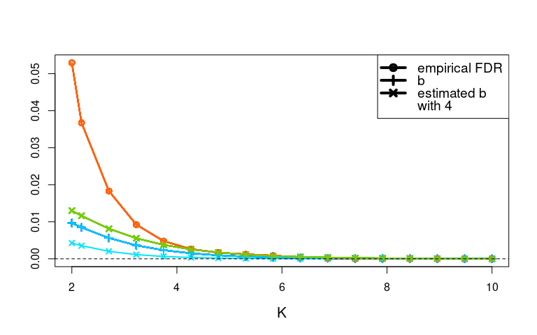
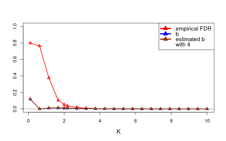
Figure 5: Top: Comparison of the empirical FDR, the function $b(K,\beta^{*},\sigma^{2})$ for the orthogonal design matrix $X$ and the function $b(K,\hat{\beta}_{\hat{m}(\tilde{K})},\hat{\sigma}^{2})$ with respectively $\hat{\beta}_{\hat{m}(1)}$, $\hat{\beta}_{\hat{m}(1.5)}$, $\hat{\beta}_{\hat{m}(2)}$, $\hat{\beta}_{\hat{m}(2.5)}$, $\hat{\beta}_{\hat{m}(3)}$, $\hat{\beta}_{\hat{m}(3.5)}$, $\hat{\beta}_{\hat{m}(4)}$, $\hat{\beta}_{\hat{m}(4.5)}$, $\hat{\beta}_{\hat{m}(5)}$ and $\hat{\beta}_{\hat{m}(\log(n))}$. The curves for $\tilde{K}\geq 2$ are indistinguishable. The terms $b(K,\hat{\beta}_{\hat{m}(\tilde{K})},\hat{\sigma}^{2})$ are calculating from only one dataset, independent of those used for the empirical estimations; for a better readability, we plot curves only for $K\geq 2$. Bottom: Same comparison and estimation only with $\tilde{K}=4$.

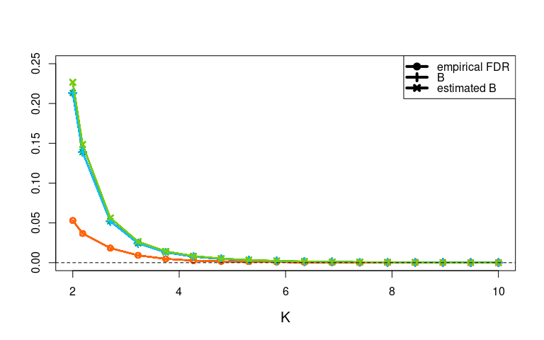
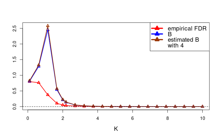
Figure 6: Top: Comparison of the empirical FDR, the function $B(K,\beta^{*},\sigma^{2})$ for the orthogonal design matrix $X$ and the function $B(K,\hat{\beta}_{\hat{m}(\tilde{K})},\hat{\sigma}^{2})$ with respectively $\hat{\beta}_{\hat{m}(1)}$, $\hat{\beta}_{\hat{m}(1.5)}$, $\hat{\beta}_{\hat{m}(2)}$, $\hat{\beta}_{\hat{m}(2.5)}$, $\hat{\beta}_{\hat{m}(3)}$, $\hat{\beta}_{\hat{m}(3.5)}$, $\hat{\beta}_{\hat{m}(4)}$, $\hat{\beta}_{\hat{m}(4.5)}$, $\hat{\beta}_{\hat{m}(5)}$ and $\hat{\beta}_{\hat{m}(\log(n))}$. The curves for $\tilde{K}\geq 2$ are indistinguishable. The terms $B(K,\hat{\beta}_{\hat{m}(\tilde{K})},\hat{\sigma}^{2})$ are calculating from only one dataset, independent of those used for the empirical estimations; for a better readability, we plot curves only for $K\geq 2$. Bottom: Same comparison and estimation only with $\tilde{K}=4$.

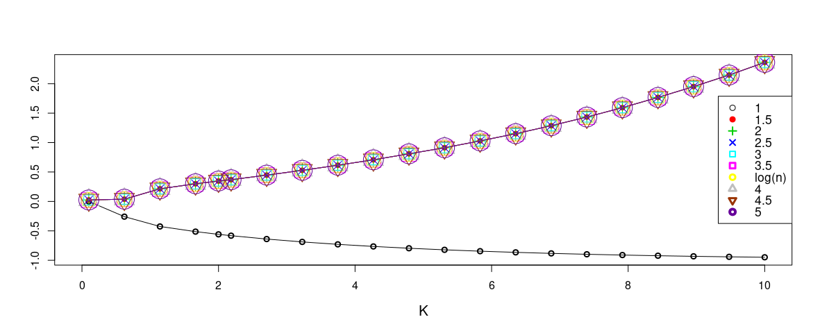
Figure 7: Curves of the relative change values between the function $b(K,\beta^{*},\sigma^{2})$ and the functions $b(K,\hat{\beta}_{\hat{m}(\tilde{K})},\hat{\sigma}^{2})$ with respectively $\hat{\beta}_{\hat{m}(1)}$, $\hat{\beta}_{\hat{m}(1.5)}$, $\hat{\beta}_{\hat{m}(2)}$, $\hat{\beta}_{\hat{m}(2.5)}$, $\hat{\beta}_{\hat{m}(3)}$, $\hat{\beta}_{\hat{m}(3.5)}$, $\hat{\beta}_{\hat{m}(4)}$, $\hat{\beta}_{\hat{m}(4.5)}$, $\hat{\beta}_{\hat{m}(5)}$ and $\hat{\beta}_{\hat{m}(\log(n))}$, where estimators are calculated from only one dataset.

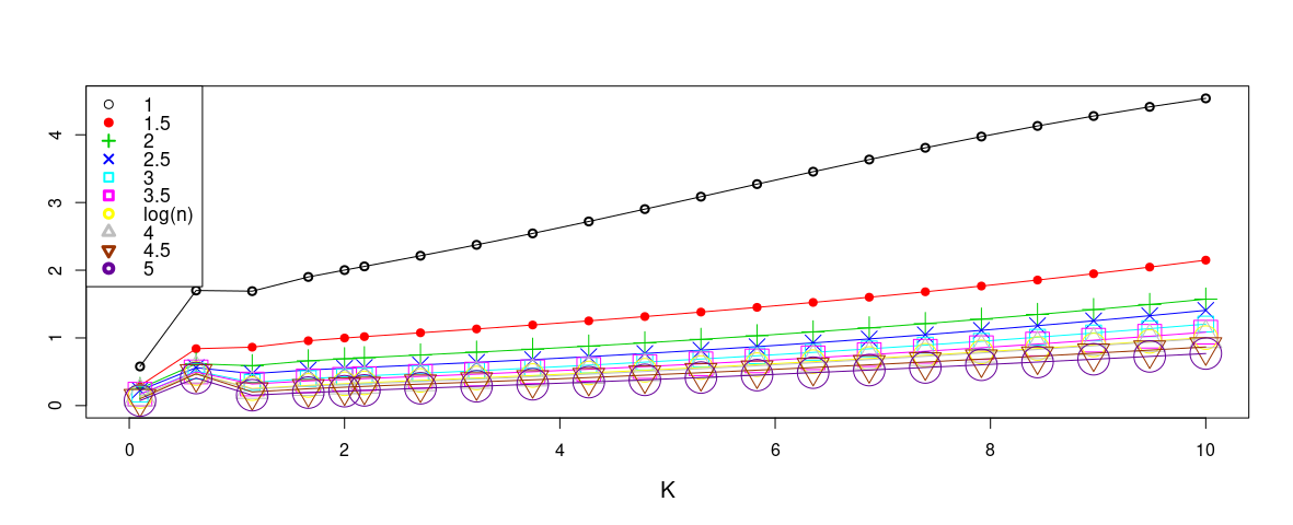
Figure 8: Curves of the relative standard deviation (standard deviation normalized by the mean) of the functions $b(K,\hat{\beta}_{\hat{m}(\tilde{K})},\hat{\sigma}^{2})$ obtained from $100$ data sets. With each one, $\hat{\beta}_{\hat{m}(1)},\hat{\beta}_{\hat{m}(1.5)},\hat{\beta}_{\hat{m}(2)},\hat{\beta}_{\hat{m}(2.5)},\hat{\beta}_{\hat{m}(3)},\hat{\beta}_{\hat{m}(3.5)},\hat{\beta}_{\hat{m}(4)},\hat{\beta}_{\hat{m}(4.5)},\hat{\beta}_{\hat{m}(5)}$ and $\hat{\beta}_{\hat{m}(\log(n))}$ are calculated given $b(K,\hat{\beta}_{\hat{m}(\tilde{K})},\hat{\sigma}^{2})$, variance of the $100$ $b(K,\hat{\beta}_{\hat{m}(\tilde{K})},\hat{\sigma}^{2})$ functions and then the relative standard deviation with respect to $K$.

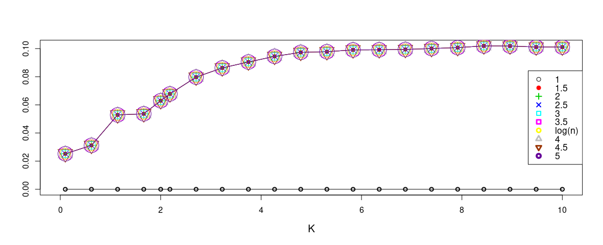
Figure 9: Curves of the relative change values between the function $B(K,\beta^{*},\sigma^{2})$ and the functions $B(K,\hat{\beta}_{\hat{m}(\tilde{K})},\hat{\sigma}^{2})$ with respectively $\hat{\beta}_{\hat{m}(1)}$, $\hat{\beta}_{\hat{m}(1.5)}$, $\hat{\beta}_{\hat{m}(2)}$, $\hat{\beta}_{\hat{m}(2.5)}$, $\hat{\beta}_{\hat{m}(3)}$, $\hat{\beta}_{\hat{m}(3.5)}$, $\hat{\beta}_{\hat{m}(4)}$, $\hat{\beta}_{\hat{m}(4.5)}$, $\hat{\beta}_{\hat{m}(5)}$ and $\hat{\beta}_{\hat{m}(\log(n))}$, where estimators are calculated from only one dataset.

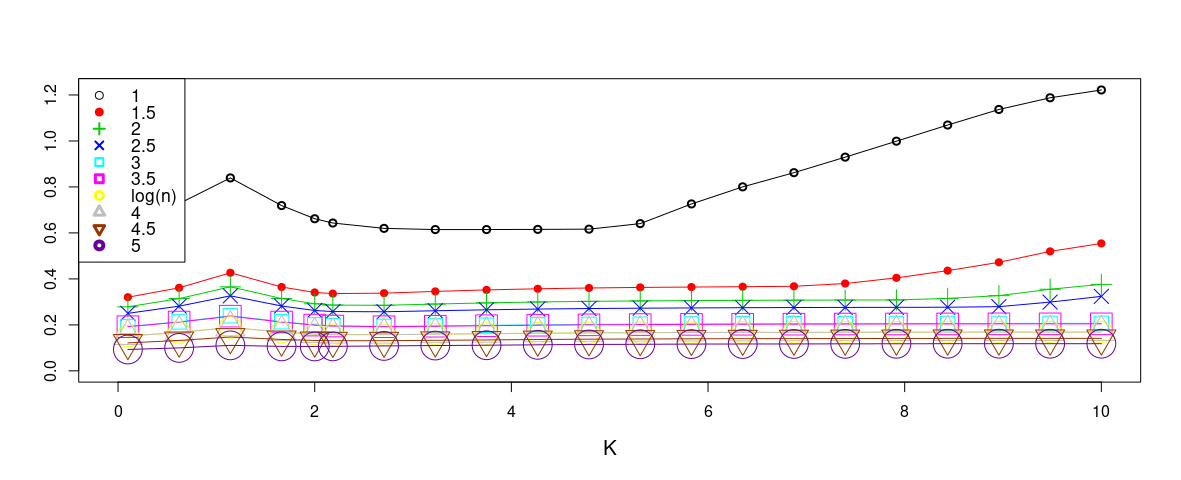
Figure 10: Curves of the relative standard deviation (standard deviation normalized by the mean) of the functions $B(K,\hat{\beta}_{\hat{m}(\tilde{K})},\hat{\sigma}^{2})$ obtained from $100$ data sets. With each one, $\hat{\beta}_{\hat{m}(1)},\hat{\beta}_{\hat{m}(1.5)},\hat{\beta}_{\hat{m}(2)},\hat{\beta}_{\hat{m}(2.5)},\hat{\beta}_{\hat{m}(3)},\hat{\beta}_{\hat{m}(3.5)},\hat{\beta}_{\hat{m}(4)},\hat{\beta}_{\hat{m}(4.5)},\hat{\beta}_{\hat{m}(5)}$ and $\hat{\beta}_{\hat{m}(\log(n))}$ are calculated given $B(K,\hat{\beta}_{\hat{m}(\tilde{K})},\hat{\sigma}^{2})$, variance of the $100$ $B(K,\hat{\beta}_{\hat{m}(\tilde{K})},\hat{\sigma}^{2})$ functions and then the relative standard deviation with respect to $K$.

for the upper bound. To ensure that $B(K,\hat{\beta}_{\hat{m}(\tilde{K})},\hat{\sigma}^{2})$ values are larger than the $B(K,\beta^{*},\sigma^{2})$ values and so larger than the FDR ones, positive relative change values and as close to $0$ as possible are expected. Concerning the lower bounds, negative relative change values are expected to ensure that $b(K,\hat{\beta}_{\hat{m}(\tilde{K})},\hat{\sigma}^{2})$ values are smaller than $B(K,\beta^{*},\sigma^{2})$ values and so smaller than the FDR ones. To take into account randomness of the $b(K,\hat{\beta}_{\hat{m}(\tilde{K})},\hat{\sigma}^{2})$ and $B(K,\hat{\beta}_{\hat{m}(\tilde{K})},\hat{\sigma}^{2})$ terms, we evaluate for all $K$ the relative standard deviation, defined by the standard deviation divided by the mean, by calculated the variance of bounds $b(K,\hat{\beta}_{\hat{m}(\tilde{K})},\hat{\sigma}^{2})$ and $B(K,\hat{\beta}_{\hat{m}(\tilde{K})},\hat{\sigma}^{2})$ evaluated on $100$ new data sets generated independently of $\mathcal{D}$. The relative standard deviation values are expected to be as close to $0$ as possible.
Figures 5-10 are plotted from the toy data set. In Figures 5 and 6, the empirical estimation of the $\text{FDR}\big{(}\hat{m}(K)\big{)}$ and the quantities $b(K,\beta^{*},\sigma^{2})$, $B(K,\beta^{*},\sigma^{2})$, $b(K,\hat{\beta}_{\hat{m}(\tilde{K})},\hat{\sigma}^{2})$ and $B(K,\hat{\beta}_{\hat{m}(\tilde{K})},\hat{\sigma}^{2})$ are plotted on a grid of positive $K$. Relative changes and relative standard deviations for the lower bounds $b(K,\hat{\beta}_{\hat{m}(\tilde{K})},\hat{\sigma}^{2})$ are plotted in Figures 7 and 8. Relative changes and relative standard deviations for the upper bounds $B(K,\hat{\beta}_{\hat{m}(\tilde{K})},\hat{\sigma}^{2})$ are plotted in Figures 9 and 10. The graphs of all others $\mathcal{D}$ of the $4$ scenarios described in Subsection 7.1 are provided in the supplementary material available in .

The lower bounds:

For $\tilde{K}>1$, the relative change values are positive until achieving more than $2$ for large $K$ (Figure 7) and the estimated lower bounds curves can be larger than the theoretical one. The relative standard deviation functions increase quickly whatever the value of $\tilde{K}$ suggesting that fluctuations around the mean are not negligible (Figure 8).

The upper bounds:

For $\tilde{K}>1$, the relative change functions are always positive and do not exceed $0.11$ meaning that the $B(K,\hat{\beta}_{\hat{m}(\tilde{K})},\hat{\sigma}^{2})$ curves are close to $B(K,\beta^{*},\sigma^{2})$ for all $K>0$ (Figure 9). For data sets $\mathcal{D}$ other than the toy data set (Figures are available in Supplementary material ), the relative change values are always small but can be negative. However, it happens very rarely for $\tilde{K}\geq 4$ and in this case, values are low enough (smaller than $-0.02\%$) to ensure that the empirical FDR estimation curves do not exceed the $B(K,\hat{\beta}_{\hat{m}(\tilde{K})},\hat{\sigma}^{2})$ terms. Concerning the relative standard deviation functions (Figures 10), the larger $\tilde{K}$, the smaller the values, except for the scenario (ii) with the third configuration where values increase after $\tilde{K}\geq 4.5$. For $\tilde{K}\geq 3.5$, the relative standard deviation values are around $0.2$ for all the scenarios except for scenario (ii) with the second configuration (can achieve $0.8$) and with the third configuration (can achieve $1$). Thus, for a value of $\tilde{K}\in\{3.5,\log(n),4,4.5,5\}$ and eventually except for the two extreme scenarios, fluctuations around the mean are small, meaning that the upper bound estimations are stable.

To conclude, we drop the lower bound to implement our data-driven algorithm for hyperparameter calibration since $b(K,\hat{\beta}_{\hat{m}(\tilde{K})},\hat{\sigma}^{2})$ functions can be larger than the theoretical FDR one. To control the FDR, only an upper bound control is sufficient. The best results for $B(K,\hat{\beta}_{\hat{m}(\tilde{K})},\hat{\sigma}^{2})$ are obtained with the hyperparameter $\tilde{K}=4$, where the relative change values are almost always positive, small enough to guarantee that the $B(K,\hat{\beta}_{\hat{m}(4)},\hat{\sigma}^{2})$ are larger than the theoretical FDR, and the relative standard deviation values are the smallest ones whatever the scenarios. So, the estimator used in our algorithm to replace $\beta^{*}$ in the upper bound of the FDR is $\hat{\beta}_{\hat{m}(4)}$. A natural estimator of $D_{m^{*}}$ is $D_{\hat{m}(4)}$. The value of the hyperparameter $\tilde{K}=4$ is not surprising since the value of $D_{\hat{m}}$ has to be small enough in (3.5) to get an upper bound $B(K,\hat{\beta}_{\hat{m}(\tilde{K})},\hat{\sigma}^{2})$ larger than the theoretical upper one. So, the penalization function has to be large enough in (2.2).

7.3 The complete variable selection

This subsection completes Subsection 4.3 about the assessment of our approach in complete variable selection by considering scenarios described in Table 3. Figures and tables are provided in the supplementary material available in .

Figures 29-31 (available in Supplementary material ) show similar results about the robustness to variable order. This confirms that being able to discriminate between active and non active variables is crucial. For scenario (ii), $B(K,\hat{\beta}_{\hat{m}(4)},\hat{\sigma}^{2})$ values begin to diverge from those of $B(K,\beta^{*},\sigma^{2})$ for the second and the third configurations where the coefficients of $\beta^{*}$ are close to each other. Concerning the second configuration, $B(K,\hat{\beta}_{\hat{m}(4)},\hat{\sigma}^{2})$ and $B(K,\beta^{*},\sigma^{2})$ values are both larger than the empirical FDR ones which is expected. When permutations of the first twelve and fifteen variables are processed, FDR values are, in most cases, even higher along the collections than for the toy data set, especially for scenario (ii) configuration (iii) and for scenario (iv) with $\sigma^{2}=4$ for which distinction between variables is more difficult; the PR values increase faster than for the toy data set. A meticulous study on the choice of the parameters $\gamma$ and $\alpha$ is required to get low values of both PR and FDR.
Table 1 (available in Supplementary material ) show the proportion of active variables in models of size $5$, $10$, $15$ and $20$ for random collection built with Bolasso, SLOPE, random forest and the knockoff method. Among the random model collections, the knockoff method provides the highest values for all scenarios except scenario (iv) with $\sigma^{2}=0.1$ and some models of size $20$ where Bolasso is the best method. Results deteriorate for specific scenarios: around $0.8$ for scenario (iv) with $\sigma^{2}=4$, $0.6$ for scenario (ii) with the third configuration and $0.8$ for scenario (ii) with the second configuration for which the discrimination between active and non active variables is naturally less obvious.

7.4 Application of algorithm 1

This subsection completes Subsection 4.2 and Subsection 4.4 by comparing Algorithm 1 and the three variable selection methods (presented below) on scenarios described in Table 3 and from the different considered model collections.
With the nested model collection (2.1) and with $\alpha=0.05$ and $\gamma=0.1$, algorithm 1 provides $K=2.8$ for scenario (i) with $D_{m}^{*}=20$ and $K=3.3$ for all others except for scenario (i) with $D_{m}^{*}=1$, for scenario (ii) with the second and the third configurations and for scenario (iv) with $\sigma^{2}=4$. Concerning these last four scenarios, the intersection of $I_{1}$ and $I_{2}$ is empty. The minimum of $I_{1}$ equals $4.8$ for scenario (i) with $D_{m}^{*}=1$ and for scenario (ii) with the second configuration, and equals $3.3$ for scenario (ii) with the third configuration and for scenario (iv) with $\sigma^{2}=4$. To get a non-empty intersection, $\gamma$ or $\alpha$ has to be higher. In all these examples, we observe that the value of $K$ provided by taking $\min(I_{1}\cap I_{2})$ coincides with $\min(I_{1})$, so increasing the value of $\gamma$ does not change $K$. However, increasing the value of $\alpha$ provides smaller values for $K$. When $\alpha=0.1$ and $\gamma=0.1$, the intersection of $I_{1}$ and $I_{2}$ is empty and the obtained values of $K$ from $\min(I_{1})$ are $3.8$ for scenario (i) with $D_{m}^{*}=1$ and for scenario (ii) with the second configuration and $2.8$ for scenario (ii) with the third configuration and for scenario (iv) with $\sigma^{2}=4$. Hence, these four cases are typical examples where the choice of $K$ depends strongly on the chosen balance between PR and FDR. In all cases, we always notice that whatever the given balance, the $K$ provided from algorithm 1 coincides with the one given by the trade-off between the two empirical quantities of PR and FDR.
When we compare our algorithm application with the three considered existing variable selection methods (see Tables 2-4 (available in Supplementary material )), all observations mentioned in Subsection 4.4 remain valid over the different scenarios

8 Acknowledgments

This research is supported in part by a public grant as part of the Investissement d’avenir project, reference ANR-11-LABX-0056-LMH, LabEx LMH. IPS2 benefits from the support of the LabEx Saclay Plant Sciences-SPS (ANR-17-EUR-0007).
The authors warmly thank and are grateful to Pascal Massart (Laboratoire de Mathématiques d’Orsay, Université Paris-Saclay) for helpful discussions and valuable comments. The authors would like to sincerely thank the Editor and the two anonymous referees for their valuable comments, suggestions and feedbacks which improved the paper.

9 Supplementary data

All the R scripts are available at https://github.com/PerrineLacroix/Trade_off_FDR_PR.

The graphs for the bounds $B(K,\hat{\beta}_{\hat{m}(\tilde{K})},\hat{\sigma}^{2})$ applied on the $4$ scenarios described in Subsection 7.1, as well as the study of the robustness of variable orders, of the construction of random model collections and of the comparison of our algorithm with other variable selection procedures, are provided in the supplementary material available in https://github.com/PerrineLacroix/Trade_off_FDR_PR. It is complementary to Subsections 7.2, 7.3 and 7.4.

References

- [1] Trevor Hastie, Robert Tibshirani, Jerome H Friedman, and Jerome H Friedman. The elements of statistical learning: data mining, inference, and prediction, volume 2. Springer, 2009.
- [2] R. Tibshirani. Regression shrinkage and selection via the lasso. Journal of the Royal Statistical Society: Series B (Methodological), 58(1):267–288, 1996.
- [3] Florentina Bunea, Alexandre B Tsybakov, and Marten H Wegkamp. Aggregation for gaussian regression. The Annals of Statistics, 35(4):1674–1697, 2007.
- [4] Florentina Bunea, Alexandre Tsybakov, and Marten Wegkamp. Sparsity oracle inequalities for the lasso. Electronic Journal of Statistics, 1:169–194, 2007.
- [5] N. Meinshausen and P. Bühlmann. Stability selection. Journal of the Royal Statistical Society: Series B (Statistical Methodology), 72(4):417–473, 2010.
- [6] F. Bach. Bolasso: model consistent lasso estimation through the bootstrap. In Proceedings of the 25th international conference on Machine learning, pages 33–40, 2008.
- [7] Seymour Geisser. The predictive sample reuse method with applications. Journal of the American statistical Association, 70(350):320–328, 1975.
- [8] Sylvain Arlot and Alain Celisse. A survey of cross-validation procedures for model selection. Statistics surveys, 4:40–79, 2010.
- [9] H Akaike. Information theory and an extension of maximum likelihood principle. In Proc. 2nd Int. Symp. on Information Theory, pages 267–281, 1973.
- [10] Colin L Mallows. Some comments on cp. Technometrics, 42(1):87–94, 2000.
- [11] G. Schwarz. Estimating the dimension of a model. The annals of statistics, 6(2):461–464, 1978.
- [12] J. Chen and Z. Chen. Extended bayesian information criteria for model selection with large model spaces. Biometrika, 95(3):759–771, 2008.
- [13] L. Birgé and P. Massart. Minimal penalties for gaussian model selection. Probability theory and related fields, 138(1-2):33–73, 2007.
- [14] J.P. Baudry, C. Maugis, and B. Michel. Slope heuristics: overview and implementation. Statistics and Computing, 22(2):455–470, 2012.
- [15] Y. Baraud, C. Giraud, S. Huet, et al. Gaussian model selection with an unknown variance. The Annals of Statistics, 37(2):630–672, 2009.
- [16] C. Giraud, S. Huet, N. Verzelen, et al. High-dimensional regression with unknown variance. Statistical Science, 27(4):500–518, 2012.
- [17] C Bonferroni. Teoria statistica delle classi e calcolo delle probabilita. Pubblicazioni del R Istituto Superiore di Scienze Economiche e Commericiali di Firenze, 8:3–62, 1936.
- [18] R John Simes. An improved bonferroni procedure for multiple tests of significance. Biometrika, 73(3):751–754, 1986.
- [19] Y. Benjamini and Y. Hochberg. Controlling the false discovery rate: a practical and powerful approach to multiple testing. Journal of the Royal statistical society: series B (Methodological), 57(1):289–300, 1995.
- [20] Yoav Benjamini and Daniel Yekutieli. The control of the false discovery rate in multiple testing under dependency. Annals of statistics, pages 1165–1188, 2001.
- [21] J. Storey, J. Taylor, and D. Siegmund. Strong control, conservative point estimation and simultaneous conservative consistency of false discovery rates: a unified approach. Journal of the Royal Statistical Society: Series B (Statistical Methodology), 66(1):187–205, 2004.
- [22] J. Romano, A. Shaikh, and M. Wolf. Control of the false discovery rate under dependence using the bootstrap and subsampling. Test, 17(3):417–442, 2008.
- [23] D. Leung and W. Sun. Zap: -value adaptive procedures for false discovery rate control with side information. arXiv preprint arXiv:2108.12623, 2021.
- [24] R. Barber, E. Candès, et al. Controlling the false discovery rate via knockoffs. The Annals of Statistics, 43(5):2055–2085, 2015.
- [25] Shuheng Zhou. Thresholding procedures for high dimensional variable selection and statistical estimation. Advances in Neural Information Processing Systems, 22:2304–2312, 2009.
- [26] Richard Berk, Lawrence Brown, Andreas Buja, Kai Zhang, and Linda Zhao. Valid post-selection inference. The Annals of Statistics, pages 802–837, 2013.
- [27] J. Lee, D. Sun, Y. Sun, and J. Taylor. Exact post-selection inference, with application to the lasso. The Annals of Statistics, 44(3):907–927, 2016.
- [28] S. Hyun, M. G’sell, and R. Tibshirani. Exact post-selection inference for the generalized lasso path. Electronic Journal of Statistics, 12(1):1053–1097, 2018.
- [29] Y. Chen, S. Jewell, and D. Witten. More powerful selective inference for the graph fused lasso, 2021.
- [30] V. Duy and I. Takeuchi. More powerful conditional selective inference for generalized lasso by parametric programming. arXiv preprint arXiv:2105.04920, 2021.
- [31] Dongliang Zhang, Abbas Khalili, and Masoud Asgharian. Post-model-selection inference in linear regression models: An integrated review. Statistics Surveys, 16:86–136, 2022.
- [32] C. Genovese and L. Wasserman. Operating characteristics and extensions of the false discovery rate procedure. Journal of the Royal Statistical Society: Series B (Statistical Methodology), 64(3):499–517, 2002.
- [33] C. Genovese, L. Wasserman, et al. A stochastic process approach to false discovery control. The Annals of Statistics, 32(3):1035–1061, 2004.
- [34] F. Abramovich, Y. Benjamini, D. Donoho, I. Johnstone, et al. Adapting to unknown sparsity by controlling the false discovery rate. The Annals of Statistics, 34(2):584–653, 2006.
- [35] M. Bogdan, E. Berg, W. Su, and E. Candes. Statistical estimation and testing via the sorted l1 norm. arXiv preprint arXiv:1310.1969, 2013.
- [36] Weijie Su and Emmanuel Candes. Slope is adaptive to unknown sparsity and asymptotically minimax. 2016.
- [37] Michał Kos and Małgorzata Bogdan. On the asymptotic properties of slope. Sankhya A, 82(2):499–532, 2020.
- [38] Peter J Bickel and Elizaveta Levina. Regularized estimation of large covariance matrices. 2008.
- [39] Elizaveta Levina, Adam Rothman, and Ji Zhu. Sparse estimation of large covariance matrices via a nested lasso penalty. 2008.
- [40] Jianhua Z Huang, Naiping Liu, Mohsen Pourahmadi, and Linxu Liu. Covariance matrix selection and estimation via penalised normal likelihood. Biometrika, 93(1):85–98, 2006.
- [41] Bin Li, J Friedman, R Olshen, and C Stone. Classification and regression trees (cart). Biometrics, 40(3):358–361, 1984.
- [42] Alexandros Kalousis, Julien Prados, and Melanie Hilario. Stability of feature selection algorithms: a study on high-dimensional spaces. Knowledge and information systems, 12:95–116, 2007.
- [43] Leo Breiman. Random forests. Machine learning, 45:5–32, 2001.
- [44] Y. Yang. Can the strengths of aic and bic be shared? a conflict between model indentification and regression estimation. Biometrika, 92(4):937–950, 2005.
- [45] L. Birgé and P. Massart. Gaussian model selection. Journal of the European Mathematical Society, 3(3):203–268, 2001.
- [46] B. Efron, T. Hastie, I. Johnstone, and R. Tibshirani. Least angle regression. The Annals of statistics, 32(2):407–499, 2004.
- [47] Isabelle Guyon, Jason Weston, Stephen Barnhill, and Vladimir Vapnik. Gene selection for cancer classification using support vector machines. Machine learning, 46:389–422, 2002.
- [48] Baptiste Gregorutti, Bertrand Michel, and Philippe Saint-Pierre. Correlation and variable importance in random forests. Statistics and Computing, 27:659–678, 2017.
- [49] David M Allen. The relationship between variable selection and data agumentation and a method for prediction. technometrics, 16(1):125–127, 1974.
- [50] Mervyn Stone. Cross-validatory choice and assessment of statistical predictions. Journal of the royal statistical society: Series B (Methodological), 36(2):111–133, 1974.
- [51] Jun Shao. Linear model selection by cross-validation. Journal of the American statistical Association, 88(422):486–494, 1993.
- [52] Frank R Kschischang. The complementary error function. Online, April, 2017.
- [53] Beatrice Laurent and Pascal Massart. Adaptive estimation of a quadratic functional by model selection. Annals of Statistics, pages 1302–1338, 2000.