Signatures of two- and three-dimensional semimetals from circular dichroism
Abstract
Topological invariants are crucial quantities for classifying materials with topological phases. Hence, their connections with experimentally measurable quantities are extremely important. In this context, circular dichroism (CD) provides a protocol to detect the Chern number of the lowest energy Bloch band (LBB) of a semimetal. This hinges on the unequal depletion rates of the Bloch electrons from a filled LBB, under the action of a time-periodic circular drive, depending on the chirality of the polarization. According to the dimensionality of the system (i.e., whether it is two- or three-dimensional), the integrated differential rate for depletion has to be formulated a bit differently in order to relate it to . Our aim is to capture the nature of the CD response for semimetals with anisotropic band dispersions. We show that while the quantization of the CD response for the three-dimensional cases is strongly sensitive to anisotropy, the two-dimensional counterparts show a perfectly quantized response.
I Introduction
A Berry phase is a geometrical phase angle that describes how a global phase accumulates over the course of a cycle, as some complex vector is transported around a closed loop in a complex vector space [1, 2, 3]. Berry phases manifest themselves in a rich variety of physical contexts including classical optics, atomic and molecular physics, nuclear physics, photonics, and condensed-matter physics. The Berry connection is the local gauge field (analogous to the vector potential) associated with the Berry phase, whose exterior derivative gives us the Berry curvature (BC). The BC turns out to be the imaginary part of the quantum geometric tensor [4]. The integral of the BC over a closed manifold is quantized in units of , and is referred to as the Chern number.
In solid state physics, the Berry phase enters into the quantum-mechanical band theory of electrons in crystals, and the complex vector in question is a Bloch wavevector, such that the closed path lies in the space of wavevectors within the Brillouin zone. As a result, the Chern number is defined entirely in terms of the momentum space wave functions, and has emerged as an important tool to classify topological phases of matter.
Over the past few years, the impact of BC on various transport phenomena has attracted tremendous interest. Some examples include anomalous Hall effect [5], Magnus Hall effect [6, 7, 8], negative magnetoresistance [9, 10], nonlinear Hall effect [11], planar Hall effect [12, 13, 14], circular photogalvanic effect [15, 16, 17], circular dichroism [18, 19, 20, 21], and second-order photoconductivities in terms of geometrical quantities [22].
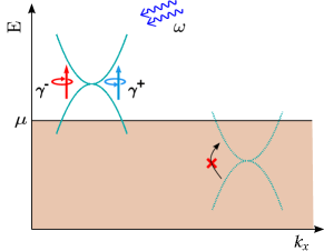
In recent times, several techniques [23, 24, 25] across diverse platforms have been proposed to detect the Chern numbers of the Bloch bands. Among them, “circular dichroism” (CD) is a response under a circular time-periodic perturbation [19, 20, 26] (for example, by shining circularly polarized light). The phenomenon hinges on the fact that the depletion rate of the filled bands in a topological phase, under the effects of an external drive, depends on the orientation (handedness) of the circular shake. The chiral nature of the system causes it to have unequal depletion rates depending on whether the drive is left- or right-handed.111This chirality is in analogy with the chiral Majorana quasiparticles that appear at the edges of topological nanowires [27, 28, 29, 30, 31, 32]. In the context of the semimetals, the sign of the topological charge (or in turn, the chirality) can be related to the chiral edge states observed in various experiments [33]. This central idea behind the CD response is depicted schematically in Fig. 1. Circular drives, confined to a two-dimensionsional (2d) plane, can be realized through circular shaking in ultracold atoms trapped in optical lattices [34], using piezo-electric actuators [35] — this activates transitions involving momentum components (of the Bloch states) confined to that particular 2d plane. In fact, this technique has been implemented to measure the Chern numbers of systems like the two-band Haldane model [19] and topological floquet bands [26]. Furthermore, a similar technique with linear shaking has been proposed [36] to probe the quantum metric tensor in periodically driven systems.
In 2d systems, the net depletion rate integrated over the momenta and frequency domain yields a quantized observable dubbed as the “differential integrated rate” (DIR), and is proportional to the Chern number of the lowest energy Bloch band [19]. The quantized response has been demonstrated in a variety of systems like 2d topological insulators, transition metal dichalcogenides [37], 2d quantum magnets [38], as well as amorphous systems [39].
In our earlier paper [21], we have formulated the CD response for three-dimensional (3d) systems. The prescription involves computing the product of the net depletion rate and the difference of band velocities, which is then integrated over the 3d Brillouin zone. We call this quantity the 3d DIR, which is found to be quantized for topological semimetals having isotropic dispersions. However, the quantization is found to be strongly affected if anisotropies are included. With this backdrop, we compute the CD responses for both 2d and 3d anisotropic semimetals. Specifically, we consider multi-Weyl [40] and semi-Dirac [41, 42] semimetals that feature anisotropic dispersions. Although band-touching nodes always come in pairs due to the Nielsen-Ninomiya theorem [43], with each pair featuring opposite chiralities, here we consider a single isolated node for computing the CD. This is because if the inversion and mirror symmetries are broken, conjugate nodes with opposite chiralities appear at different energies [44], in which case we can Pauli-block the one at lower energies by adjusting the Fermi level (cf. Fig. 1).
II Circular drive and differential integrated rates in 2d and 3d
Let us consider a circularly polarized time-periodic drive described by the Hamiltonian , where is the amplitude, is the frequency, and denote the mutually perpendicular position vector operators defining the plane of polarization of the applied drive, and the subscript “” refers to the handedness of the circular polarization. A non-interacting Hamiltonian (describing the semimetal in question) is subjected to this perturbation, such that the total Hamiltonian is given by
| (1) |
It is convenient to use a unitary transformation to bring the Hamiltonian to a translation-invariant form [19, 36]. In addition, we assume small driving amplitudes [where is the reduced Planck’s constant], because the drive is treated as a perturbation. Incorporating these ingredients, the final Hamiltonian takes the form:
| (2) |
to leading order in .
For a two-band Hamiltonian, at the initial time , we consider having a system with the lower energy Bloch band (with eigenvalue and eigenstate ) filled. Then on switching on the periodic drive starting from , transitions of the Bloch electrons to the upper band (with eigenvalue and eigenstate ) are activated. This leads to a “depletion rate” of the occupied Bloch band — a pivotal quantity of the CD protocol. Using the Fermi’s golden rule [45], the depletion rate for sufficiently long time scales is given by
| (3) |
where is the optical matrix element. Here, represents the energy difference between the higher and the lower energy bands. Henceforth, we abbreviate the lowest energy Bloch band as LBB.
Clearly, the presence of the delta function in our analytical expression forces the photon energy to precisely match with the band energy difference . But in practice, the transitions of course take place within a short energy window. Thus we adopt the definition of the delta function as a limit of a Lorentzian: , and approximate this as a Lorentzian with a small width in our numerics.222Specifically, we have set in obtaining all the plots. The 2d differential integrated rate (or DIR) is obtained by integrating the net depletion rate over the -space and frequency, and takes the form [19, 20, 26]:
| (4) | ||||
| (5) |
The above expression shows that the 2d DIR is quantized in units of , being proportional to the LBB Chern number .
In order to compute the 3d DIR [21], we need to consider the fact that the normal to the plane of the circular drive can be oriented along one of the three mutually perpendicular Cartesian coordinate axes. Hence, we multiply the net depletion rate (for the polarization of the drive confined to the -plane) with the component of in the perpendicular direction, where is the difference of the band velocities. Additionally, the integration is done over the 3d momnetum space only, which renders the integrated rate as a function of as shown below:
| (6) |
Here, the Levi-Civita symbol denotes cyclic permutation. For semimetals having isotropic dispersions, the 3d DIR has been shown to take the simple form [21]:
| (7) |
Hence, is always quantized [in units of ] for an isotropic two-band model.
For a generic multiband system (here more than two bands might be present), the 3d DIR formula for an isotropic system can be expressed as [21]
| (8) |
using the Stoke’s theorem, with denoting an infinitesimal area vector of the surface integral over the surface . Here, we have used the index to label all the bands in the system (with denoting the first higher energy band above the LBB, with the latter labelled as ), and have considered the situation when the LBB is filled at time . We note that the second term is relevant only in a system with more than two bands (as in the summation there), and hence it drops out for a two-band system [thus reducing to the expression in Eq. (7)].
III Numerical results
In this section, we compute the CD response for various 2d and 3d semimetals having two bands crossing at nodal points or closed nodal curves. The continuum Hamiltonians representing the semimetals are only approximations of actual lattice Hamiltonians in the low-energy limits. Hence, the momentum variables appearing in the integrals require a physical cutoff. In our numerics, we define an isotropic momentum cutoff , upto which the continuum approximation remains to a reasonable approximation. For the frequency integrals, we have set the upper limit to . In addition, we have chosen natural units (i.e., we have set ) for simplicity.
In all our examples, we consider a single node (and set its chirality to have the positive value), without any loss of generality, as it is a valid approximation for materials with well-resolved nodes in momentum space (e.g., in [46]). For the two-band models that we consider in this section, we can rewrite the Hamiltonian as , where denotes the vector comprising the three coefficients appearing against the three Pauli matrices. using this form, the Berry curvature of the LBB is simply given by the formula
| (9) |
III.1 Semi-Dirac semimetal
Semi-Dirac semimetals are 2d systems having a quadratic dispersion in one direction and a linear dispersion along the orthogonal direction [41, 42, 47, 48, 49]. Promising candidates for such semi-Dirac systems include multilayered / nanostructures [41, 42, 47], organic salts [50, 51], and deformed graphene [52, 53, 54, 55]. The low-energy continuum model Hamiltonian describing a semi-Dirac material is captured by [47, 54, 55, 48]
| (10) |
where is the quasiparticle mass along the -direction, is the Dirac velocity along the -direction, and the parameter has the dimensions of energy. We scale our Hamiltonian by (where is a momentum scale) such that energy is measured in units of , mass is measured in units of , and each momentum component is measured in units of . The system is in a (i) gapped (i.e., trivially insulating) state for ; (ii) gapless semi-Dirac phase at ; and (iii) semimetal phase for with two gapless Dirac nodes located at . We set in all our computations.
To , we add momentum-dependent symmetry-breaking terms of the form [48]
| (11) |
where has the dimensions of energy and has the units of velocity. With this additional term, the full Hamiltonian is
| (12) |
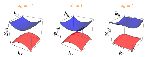
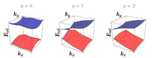
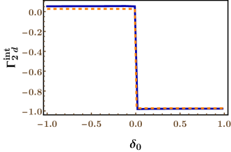
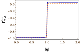
The additional terms and break the particle-hole and time-reversal symmetries, respectively. In the , the system remains in the gapped state, which is a trivial insulator (i.e., with zero Chern number). However, the regime hosts topological insulators with different Chern numbers, as the gap closes at , on tuning the value of . In particular, gives a nontrivial topological phase with , whereas corresponds to a trivial phase with . These features are demonstrated in Fig. 2. Henceforth, we set for the sake of simplicity.
From Eq. (12), can be obtained directly from the Berry curvature of the LBB, which reads
| (13) |
for and . The 2d DIR, computed numerically using Eq. (4), is plotted in Fig. 2. It is seen to coincide with the value of , as expected. A momentum cutoff value of has been used to obtain converging values in the integrals.
III.2 Multi-Weyl semimetals
In this subsection, we compute the 3d DIR for 3d nodal-point semimetals. We choose to focus on multi-Weyl semimetals [40] to understand the role of anisotropy in CD responses, as these two-band systems feature a mix of linear and higher-order dispersions, depending on the direction. They are generalizations of the Weyl semimetals (WSMs), featuring linear-in-momentum isotropic dispersions, to higher-order-in-momentum dispersions in certain directions. For the sake of comparison, we also investigate the corresponding behaviour of their isotropic counterparts, which have the same higher-order dispersion in all directions.
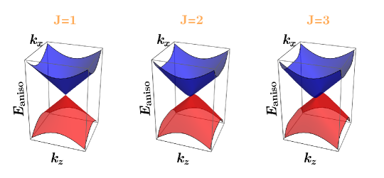
The low-energy continuum model of a multi-WSM is given by
| (14) |
where and . The velocities and describe the Fermi velocities along the -plane and along the -axis, respectively, and is a material-dependent parameter with the dimensions of momentum. We set for the sake of simplicity. The topological charge of a positive chirality multi-Weyl node is described by the integer , with the case simply capturing the WSM. The eigenvalues of the Hamiltonian are given by , revealing quadratic and cubic dispersions in the -plane, for a double-WSM (with ) and a triple-WSM (with ), respectively. We note that a WSM-like linear dispersion persists along the -direction. Several first-principle calculations predict the existence of double-WSM in [56], while certain transition-metal monochalcogenides have been proposed as examples of triple-WSM behaviour [57].
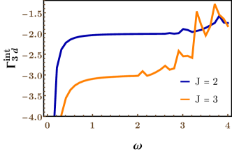
We scale our Hamiltonian by such that mass and energy are measured in units of , and each momentum component is measured in units of . We compare the 3d DIR results [computed using Eq. (II)] with the values of (computed from the BC), noting that
| (15) |
This gives . The 3d DIR response for is shown as a function of drive frequency in Fig. 3(a). A momentum cutoff value of has been used to obtain converging values in the integrals. As expected from Eq. (7), the WSM exhibits a quantized response [cf. the case in Fig. 3(c)]. Due to anisotropy, such perfect quantization does not exist for throughout the frequency domain — the response is quantized for a limited frequency range, and as the frequency increases beyond a critical value, the response decays from the quantized plateau to eventually become zero. We note that the rate of decay is faster for higher value of . This can be understood if we consider the fact that quantization of DIR is highly sensitive to the magnitude of anisotropy. With increasing driving frequency, photons probe the higher and higher energy ranges, where the effects of anisotropy are greater. And these effects grow more rapidly with the increasing power of momentum in the nonlinearly dispersing directions. This, in turn, destroys the quantization faster.
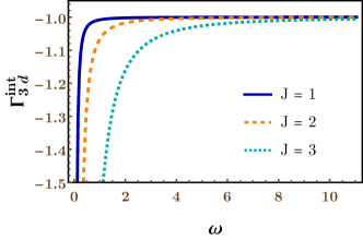
We now compare the response seen for the multi-WSMs with that of the corresponding isotropic cases, which have the same higher power-law dependence on as seen for the multi-WSMs on in the -plane. Hence, we consider the Hamiltonian [58]
| (16) |
with energy eigenvalues . Here, and are again material-dependent parameters and we scale the Hamiltonian by the factor as before. Irrespective of the value of , for these isotropic systems, since . The 3d DIR response is shown as a function of the drive frequency in Fig. 3(c), which indeed shows saturation to the value of in units of . However, we note that the value of , at which saturation is reached, increases with increasing nonlinearity of the dispersion.
IV Summary and outlook
In this paper, we have investigated circular dichroism for nodal-point semimetals harbouring nontrivial topological charges. The response is initiated by a circular periodic drive, which causes transitions from a filled band to higher energy bands. The circularly dichroic response is caused by unequal transition rates connected with the chiral nature of the systems.
We would like to emphasize that the 3d DIR response [21] (applicable for 3d systems) is different from the 2d DIR formula [19] (apllicable for 2d systems). For computing , the net transition rate is computed for each 2d projection of the 3d system, which is confined to the -plane. With denoting the direction perpendicular to this 2d plane under consideration, we then multiply with the band velocity difference , and integrate it over the entire 3d Brillouin zone to get the differential current along the direction. This is followed by a summation over the three mutually perpendicular directions. This complicated expression happens to overlap with the expression of the Chern number of the LBB, at leading order, only for systems with isotropic dispersions [21]. We also note that is a function of (i.e., integration over is not performed while deriving it). On the other hand, is obtained by integrating over a frequency interval.
For 3d systems with isotropic dispersions (both linear and nonlinear), the 3d DIR exhibits a quantized response in terms of the LBB Chern number. This robust quantization persists throughout the frequency domain, and is absent for anisotropic multi-WSMS (with ), which feature quadratic (for ) and cubic (for ) dispersions in the plane perpendicular to the -axis (in our choice of coordinate system). Instead, the multi-WSMs show a small quantized plateau followed by a non-quantized response, which decays to zero as increases.
For the 2d semimetals, the 2d DIR response does not depend on anisotropy. The analytical expression in fact shows that it is always proportional to the Chern number of the filled band, and this is what we find in our numerical results as well.
Our CD computations complement earlier studies of DIR on various systems [19, 21]. The DIR response also supplements other techniques, involving time-periodic drives, to characterize topological phases [22, 59, 60, 14]. In future, it will be worthwhile to study the CD response in the presence of interactions and/or impurities [61, 62, 63, 64, 65]. The presence of very strong interactions may induce many-body effects like (i) destroying the quantization of topological charges like Chern numbers [16, 17]; (ii) emergence of strongly correlated phases [66, 67, 61, 62, 63, 64], where the quasiparticle picture breaks down.
Acknowledgments
We thank Soustav Bose and Sajid Sekh for participating in the preliminary stages of this work.
References
- Pancharatnam [1956] S. Pancharatnam, Generalized theory of interference, and its applications, Proceedings of the Indian Academy of Sciences - Section A 44, 247 (1956).
- Berry [1984] M. V. Berry, Quantal phase factors accompanying adiabatic changes, Proceedings of the Royal Society of London. A. Mathematical and Physical Sciences 392, 45 (1984).
- Wilczek and Shapere [1989] F. Wilczek and A. Shapere, Geometric Phases in Physics (World Scientific, 1989) pp. 7–28.
- Vanderbilt [2018] D. Vanderbilt, Berry Phases in Electronic Structure Theory: Electric Polarization, Orbital Magnetization and Topological Insulators (Cambridge University Press, 2018).
- Nagaosa et al. [2010] N. Nagaosa, J. Sinova, S. Onoda, A. H. MacDonald, and N. P. Ong, Anomalous Hall effect, Rev. Mod. Phys. 82, 1539 (2010).
- Papaj and Fu [2019] M. Papaj and L. Fu, Magnus Hall effect, Phys. Rev. Lett. 123, 216802 (2019).
- Mandal et al. [2020] D. Mandal, K. Das, and A. Agarwal, Magnus Nernst and thermal Hall effect, Phys. Rev. B 102, 205414 (2020).
- Sekh, Sajid and Mandal, Ipsita [2022] Sekh, Sajid and Mandal, Ipsita, Magnus Hall effect in three-dimensional topological semimetals, Eur. Phys. J. Plus 137, 736 (2022).
- Li et al. [2017] Y. Li, Z. Wang, P. Li, X. Yang, Z. Shen, F. Sheng, X. Li, Y. Lu, Y. Zheng, and Z.-A. Xu, Negative magnetoresistance in Weyl semimetals NbAs and NbP: Intrinsic chiral anomaly and extrinsic effects, Frontiers of Physics 12, 127205 (2017).
- Dai et al. [2017] X. Dai, Z. Z. Du, and H.-Z. Lu, Negative magnetoresistance without chiral anomaly in topological insulators, Phys. Rev. Lett. 119, 166601 (2017).
- He and Weng [2021] Z. He and H. Weng, Giant nonlinear Hall effect in twisted bilayer WTe2, npj Quantum Materials 6, 101 (2021).
- Nandy et al. [2017] S. Nandy, G. Sharma, A. Taraphder, and S. Tewari, Chiral anomaly as the origin of the planar Hall effect in Weyl semimetals, Phys. Rev. Lett. 119, 176804 (2017).
- Nag and Nandy [2020] T. Nag and S. Nandy, Magneto-transport phenomena of type-I multi-Weyl semimetals in co-planar setups, Journal of Physics: Condensed Matter 33, 075504 (2020).
- Yadav et al. [2022] S. Yadav, S. Fazzini, and I. Mandal, Magneto-transport signatures in periodically-driven Weyl and multi-Weyl semimetals, Physica E Low-Dimensional Systems and Nanostructures 144, 115444 (2022).
- de Juan et al. [2017] F. de Juan, A. G. Grushin, T. Morimoto, and J. E. Moore, Quantized circular photogalvanic effect in Weyl semimetals, Nature Communications 8, 15995 (2017).
- Avdoshkin et al. [2020] A. Avdoshkin, V. Kozii, and J. E. Moore, Interactions remove the quantization of the chiral photocurrent at Weyl points, Phys. Rev. Lett. 124, 196603 (2020).
- Mandal [2020] I. Mandal, Effect of interactions on the quantization of the chiral photocurrent for double-Weyl semimetals, Symmetry 12, 919 (2020).
- Roy Karmakar et al. [2021] A. Roy Karmakar, S. Nandy, G. P. Das, and K. Saha, Probing mirror anomaly and classes of Dirac semimetals with circular dichroism, Phys. Rev. Res. 3, 013230 (2021).
- Tran et al. [2017] D. T. Tran, A. Dauphin, A. G. Grushin, P. Zoller, and N. Goldman, Probing topology by “heating”: Quantized circular dichroism in ultracold atoms, Science Advances 3, e1701207 (2017).
- Midtgaard et al. [2020] J. M. Midtgaard, Z. Wu, N. Goldman, and G. M. Bruun, Detecting chiral pairing and topological superfluidity using circular dichroism, Phys. Rev. Research 2, 033385 (2020).
- Sekh and Mandal [2022] S. Sekh and I. Mandal, Circular dichroism as a probe for topology in three-dimensional semimetals, Phys. Rev. B 105, 235403 (2022).
- Hsu et al. [2023] H.-C. Hsu, J.-S. You, J. Ahn, and G.-Y. Guo, Nonlinear photoconductivities and quantum geometry of chiral multifold fermions, Phys. Rev. B 107, 155434 (2023).
- Dai et al. [2016] X. Dai, H.-Z. Lu, S.-Q. Shen, and H. Yao, Detecting monopole charge in Weyl semimetals via quantum interference transport, Phys. Rev. B 93, 161110 (2016).
- Kourtis [2016] S. Kourtis, Bulk spectroscopic measurement of the topological charge of Weyl nodes with resonant x rays, Phys. Rev. B 94, 125132 (2016).
- Bjerngaard et al. [2020] M. Bjerngaard, B. Galilo, and A. M. Turner, Neutron scattering off Weyl semimetals, Phys. Rev. B 102, 035122 (2020).
- Asteria et al. [2019] L. Asteria, D. T. Tran, T. Ozawa, M. Tarnowski, B. S. Rem, N. Fläschner, K. Sengstock, N. Goldman, and C. Weitenberg, Measuring quantized circular dichroism in ultracold topological matter, Nature Physics 15, 449 (2019).
- Kitaev [2001] A. Y. Kitaev, 6. QUANTUM COMPUTING: Unpaired Majorana fermions in quantum wires, Physics Uspekhi 44, 131 (2001).
- Niu et al. [2012] Y. Niu, S. B. Chung, C.-H. Hsu, I. Mandal, S. Raghu, and S. Chakravarty, Majorana zero modes in a quantum Ising chain with longer-ranged interactions, Phys. Rev. B 85, 035110 (2012).
- Mandal and Tewari [2016] I. Mandal and S. Tewari, Exceptional point description of one-dimensional chiral topological superconductors/superfluids in BDI class, Physica E Low-Dimensional Systems and Nanostructures 79, 180 (2016).
- Mandal [2015] I. Mandal, Exceptional points for chiral Majorana fermions in arbitrary dimensions, EPL (Europhysics Letters) 110, 67005 (2015).
- Mandal [2016] I. Mandal, Counting Majorana bound states using complex momenta, Condensed Matter Physics 19, 33703 (2016).
- Barman Ray et al. [2021] A. Barman Ray, J. D. Sau, and I. Mandal, Symmetry-breaking signatures of multiple Majorana zero modes in one-dimensional spin-triplet superconductors, Phys. Rev. B 104, 104513 (2021).
- Howard et al. [2021] S. Howard, L. Jiao, Z. Wang, N. Morali, R. Batabyal, P. Kumar-Nag, N. Avraham, H. Beidenkopf, P. Vir, E. Liu, C. Shekhar, C. Felser, T. Hughes, and V. Madhavan, Evidence for one-dimensional chiral edge states in a magnetic Weyl semimetal Co3Sn2S2, Nature Communications 12, 4269 (2021).
- Eckardt [2017] A. Eckardt, Atomic quantum gases in periodically driven optical lattices, Rev. Mod. Phys. 89, 011004 (2017).
- Jotzu et al. [2014] G. Jotzu, M. Messer, R. Desbuquois, M. Lebrat, T. Uehlinger, D. Greif, and T. Esslinger, Experimental realization of the topological Haldane model with ultracold fermions, Nature 515, 237 (2014).
- Ozawa and Goldman [2018] T. Ozawa and N. Goldman, Extracting the quantum metric tensor through periodic driving, Phys. Rev. B 97, 201117 (2018).
- Shan [2022] W.-Y. Shan, Anomalous circular phonon dichroism in transition metal dichalcogenides, Phys. Rev. B 105, L121302 (2022).
- Viñas Boström et al. [2023] E. Viñas Boström, T. S. Parvini, J. W. McIver, A. Rubio, S. V. Kusminskiy, and M. A. Sentef, Direct optical probe of magnon topology in two-dimensional quantum magnets, Phys. Rev. Lett. 130, 026701 (2023).
- Marsal et al. [2020] Q. Marsal, D. Varjas, and A. G. Grushin, Topological Weaire–Thorpe models of amorphous matter, Proceedings of the National Academy of Sciences 117, 30260 (2020).
- Fang et al. [2012] C. Fang, M. J. Gilbert, X. Dai, and B. A. Bernevig, Multi-Weyl topological semimetals stabilized by point group symmetry, Phys. Rev. Lett. 108, 266802 (2012).
- Pardo and Pickett [2009] V. Pardo and W. E. Pickett, Half-metallic semi-Dirac-point generated by quantum confinement in TiO2/VO2 nanostructures, Phys. Rev. Lett. 102, 166803 (2009).
- Pardo and Pickett [2010] V. Pardo and W. E. Pickett, Metal-insulator transition through a semi-Dirac point in oxide nanostructures: VO2 (001) layers confined within TiO2, Phys. Rev. B 81, 035111 (2010).
- Nielsen and Ninomiya [1981] H. Nielsen and M. Ninomiya, A no-go theorem for regularizing chiral fermions, Physics Letters B 105, 219 (1981).
- Zyuzin et al. [2012] A. A. Zyuzin, S. Wu, and A. A. Burkov, Weyl semimetal with broken time reversal and inversion symmetries, Phys. Rev. B 85, 165110 (2012).
- Sakurai and Napolitano [2017] J. J. Sakurai and J. Napolitano, Modern Quantum Mechanics, 2nd ed. (Cambridge University Press, 2017).
- Chang et al. [2016] G. Chang, S.-Y. Xu, D. S. Sanchez, S.-M. Huang, C.-C. Lee, T.-R. Chang, G. Bian, H. Zheng, I. Belopolski, N. Alidoust, H.-T. Jeng, A. Bansil, H. Lin, and M. Z. Hasan, A strongly robust type II Weyl fermion semimetal state in Ta3S2, Science Advances 2, e1600295 (2016).
- Banerjee et al. [2009] S. Banerjee, R. R. P. Singh, V. Pardo, and W. E. Pickett, Tight-binding modeling and low-energy behavior of the semi-Dirac point, Phys. Rev. Lett. 103, 016402 (2009).
- Sriluckshmy et al. [2018] P. V. Sriluckshmy, K. Saha, and R. Moessner, Interplay between topology and disorder in a two-dimensional semi-Dirac material, Phys. Rev. B 97, 024204 (2018).
- Mandal and Saha [2020] I. Mandal and K. Saha, Thermopower in an anisotropic two-dimensional Weyl semimetal, Phys. Rev. B 101, 045101 (2020).
- Kobayashi et al. [2011] A. Kobayashi, Y. Suzumura, F. Piéchon, and G. Montambaux, Emergence of dirac electron pair in the charge-ordered state of the organic conductor -(bedt-ttf)2i3, Phys. Rev. B 84, 075450 (2011).
- Suzumura et al. [2013] Y. Suzumura, T. Morinari, and F. Piéchon, Mechanism of Dirac point in type organic conductor under pressure, Journal of the Physical Society of Japan 82, 023708 (2013).
- Hasegawa et al. [2006] Y. Hasegawa, R. Konno, H. Nakano, and M. Kohmoto, Zero modes of tight-binding electrons on the honeycomb lattice, Phys. Rev. B 74, 033413 (2006).
- Adroguer et al. [2016] P. Adroguer, D. Carpentier, G. Montambaux, and E. Orignac, Diffusion of Dirac fermions across a topological merging transition in two dimensions, Phys. Rev. B 93, 125113 (2016).
- Montambaux et al. [2009a] G. Montambaux, F. Piéchon, J.-N. Fuchs, and M. O. Goerbig, Merging of Dirac points in a two-dimensional crystal, Phys. Rev. B 80, 153412 (2009a).
- Montambaux et al. [2009b] G. Montambaux, F. Piéchon, J.-N. Fuchs, and M. O. Goerbig, A universal Hamiltonian for motion and merging of Dirac points in a two-dimensional crystal, The European Physical Journal B 72, 509 (2009b).
- Singh et al. [2018] B. Singh, G. Chang, T.-R. Chang, S.-M. Huang, C. Su, M.-C. Lin, H. Lin, and A. Bansil, Scientific Reports 8, 10540 (2018).
- Liu and Zunger [2017] Q. Liu and A. Zunger, Predicted realization of cubic Dirac fermion in quasi-one-dimensional transition-metal monochalcogenides, Phys. Rev. X 7, 021019 (2017).
- Ahn et al. [2016] S. Ahn, E. H. Hwang, and H. Min, Collective modes in multi-Weyl semimetals, Scientific Reports 6, 34023 (2016).
- Bera and Mandal [2021] S. Bera and I. Mandal, Floquet scattering of quadratic band-touching semimetals through a time-periodic potential well, Journal of Physics Condensed Matter 33, 295502 (2021).
- Bera et al. [2023] S. Bera, S. Sekh, and I. Mandal, Floquet transmission in Weyl/multi-Weyl and nodal-line semimetals through a time-periodic potential well, Ann. Phys. (Berlin) 535, 2200460 (2023).
- Nandkishore and Parameswaran [2017] R. M. Nandkishore and S. A. Parameswaran, Disorder-driven destruction of a non-Fermi liquid semimetal studied by renormalization group analysis, Phys. Rev. B 95, 205106 (2017).
- Mandal and Nandkishore [2018] I. Mandal and R. M. Nandkishore, Interplay of Coulomb interactions and disorder in three-dimensional quadratic band crossings without time-reversal symmetry and with unequal masses for conduction and valence bands, Phys. Rev. B 97, 125121 (2018).
- [63] I. Mandal, Fate of superconductivity in three-dimensional disordered Luttinger semimetals, .
- Mandal [2021] I. Mandal, Robust marginal Fermi liquid in birefringent semimetals, Physics Letters A 418, 127707 (2021).
- Mandal and Ziegler [2021] I. Mandal and K. Ziegler, Robust quantum transport at particle-hole symmetry, EPL (Europhysics Letters) 135, 17001 (2021).
- Mandal and Gemsheim [2019] I. Mandal and S. Gemsheim, Emergence of topological Mott insulators in proximity of quadratic band touching points, Condensed Matter Physics 22, 13701 (2019).
- Moon et al. [2013] E.-G. Moon, C. Xu, Y. B. Kim, and L. Balents, Non-Fermi-liquid and topological states with strong spin-orbit coupling, Phys. Rev. Lett. 111, 206401 (2013).