Theory of intermediate twinning and spontaneous polarization in the phase transformations of ferroelectric potassium sodium niobate

Abstract

Potassium sodium niobate is considered a prominent material system as a substitute for toxic lead-containing ferroelectric materials. It exhibits first-order phase transformations and ferroelectricity with potential applications ranging from energy conversion to innovative cooling technologies, hereby addressing urgent societal challenges. However, a major obstacle in the application of potassium sodium niobate is its multi-scale heterogeneity and the lack of understanding of its phase transition pathway and microstructure. This can be seen from the findings of Pop-Ghe 2021 et al. [1] which also reveal the occurrence of intermediate twinning during the phase transition. Here we show that intermediate twinning is a consequence of energy minimization. We employ a geometrically nonlinear electroelastic energy function for potassium sodium niobate, including the cubic-tetragonal-orthorhombic transformations and ferroelectricity. The construction of the minimizers is based on compatibility conditions which ensure continuous deformations and pole-free interfaces. These minimizers agree with the experimental observations, including laminates between the tetragonal variants under the cubic to tetragonal transformation, crossing twins under the tetragonal to orthorhombic transformation, intermediate twinning and spontaneous polarization. This shows how the full nonlinear electroelastic model provides a powerful tool in understanding, exploring and tailoring the electromechanical properties of complex ferroelectric ceramics.

1 Introduction

Ferroelectric crystals have numerous applications such as piezoelectric actuators, solid-state cooling [2, 3, 4], energy storage and energy conversion [5, 6, 7]. A material that exhibits superior piezoelectric and electromechanical properties is Pb(Zr,Ti)O₃ (PZT). Besides the exceptional ferroelectric behavior, this lead-containing state-of-the-art ferroelectric material arises critical environmental issues. The K_0.5Na_0.5NbO₃ (KNN) ceramic [8] is of increased interest, since Saito’s study revealed high piezoelectric coefficient on textured KNN [9], this lead-free material is considered one of the most promising candidates in line to replace the toxic PZT [10, 11]. KNN is a complex ferroelectric ceramic, as it crystallizes in a perovskite structure like barium titanate or lead-zirconate titanate, but exhibits multi-scale heterogeneities [12, 13] unlike the preceding examples [14]. These multi-scale heterogeneities include a shared A-site correlated to abnormal grain growth in this compound [15], as well as different diffusion velocities and vapor pressures [16, 17] and poor sinterability [18]. Abnormal grain growth is of special importance in this context, since it suppresses the potential to accurately apply design strategies for material optimization due to the induced anisotropies. In [1] during the fabrication process excess of alkali metals have been incorporated suppressing inhomogeneous grain size distribution. This fatigue-optimized KNN system, called KNN_ex, exhibits two phase transitions between an orthorhombic and tetragonal, and tetragonal to cubic phases at $\sim$ 210 °C and $\sim$ 400 °C respectively, the latter transition also marking the ferroelectric to paraelectric transition. Adding to the complexity of the material, an unexplained intermediate twinning state has been discovered in KNN_ex occurring in between the orthorhombic to tetragonal phase transformation, herein further challenging the need for thorough understanding of phase transitions dynamics in ferroelectric ceramics.

Here we study the theoretical understanding of phase transitions, intermediate twinning [1] and spontaneous polarization directions [19, 20] for KNN_ex. We employ a nonlinear electrostrictive model based on the theory of magnetostriction [21] for single crystals where finite strains are allowed. The transition from magnetostriction to electrostriction has been already performed in [22], for the ferroelectric-conductor system subjected to a dead load, where external mechanical and electrical work have been incorporated to the transformed theory of magnetostriction [21]. Examples of applications for this electroelastic model include ceramic materials, e.g. in [23, 24, 25] domain switching and the electromechanical response have been explored for barium titanate. In our case spontaneous polarization occurs due to thermal induced displacive phase transitions, which means directly replacing magnetization by polarization to the magnetoelastic energy of [21] the employed electroelastic energy is obtained. The elastic response follows geometrically nonlinear elasticity [26, 27, 28, 29] and the electrical part is based on the theory of micromagnetics developed by Brown [30]. Hence, the macroscopic to the atomistic scale is related through two distinct assumptions for the deformation and spontaneous polarization respectively. The classical Cauchy-Born hypothesis is adopted, which provides the link between the atomistic and continuous deformations, i.e. the lattice vectors deform exactly as the assigned macroscopic deformation. It’s validity is ensured by restricting the deformation in the Ericksen-Pittery neighborhood [31, 32, 27] which excludes plastic deformations and slips but includes elastic deformations and phase transitions. Furthermore, it is assumed the electric dipole field oscillates in a much larger scale than the scale of the lattice [33]. Then, the macroscopic polarization is derived as a volume average of the dipole field, where the volume lies between these two scales [34]. Therefore, the theoretical analysis for magnetic, [21, 35] and electric,[22], domains formation is inherited to the current setting.

We show that experimental observed states minimize the electrostatic energy which is a multi-well function. Elements of the wells are of the form $(\nabla{\bf y},{\bf p})$, ${\bf y}$ and ${\bf p}$ denote deformation and spontaneous polarization respectively. Here strains correspond to variants of the present phase. Assuming that spontaneous polarization directions emerge along the stretch directions a direct relation between ${\bf p}$ and $\nabla{\bf y}$ arises. Then, from X-ray diffraction measurement the explicit values of the energy wells are provided. To this end, it is shown why these observed deformations of KNN_ex [1] and polarization directions [19, 20] minimize or consist a part of minimizing sequences of the electrostatic energy. Compatibility conditions ensuring deformation continuity with discontinuous deformation gradient with divergence free polarization jump at the discontinuity interface appear to be crucial for our analysis. The most striking feature of the theory is the prediction of the interfaces between variants in the very geometrically restrictive orthorhombic phase as well as potential $180\degree domains$ formation in the same phase, figures 5 & 8 .

In section 2 some evidence about the elastic response for KNN_ex is presented with the observed cubic, tetragonal, orthorhombic phases and intermediate twining. Furthermore, some preliminary results and the definition of the electroelastic are given. In section 3 predictions of the model and comparison with experimental data are demonstrated.

2 Experiment and Model

2.1 Fatigue-improved KNN

The KNN_ex bulk samples providing the experimental basis of this work exhibit a homogeneous grain size distribution [1] and optimized fatigue behavior. Preparation was executed according to the conventional solid-state route [36, 37], incorporating excess alkali metals, an optimized fabrication route [38] and the aforementioned design strategy. Differential scanning calorimetry measurements are presented in figure 1 verifying the reliable and reproducible material property improvement through engineered reversibility. Figure 1a demonstrates the predicted stabilisation of the phase transition temperature upon repeated cycling at accelerated degeneration conditions (cf. Methods section) for exemplary KNN and fatigue-optimized KNN_ex transitioning from tetragonal to cubic (T-C).

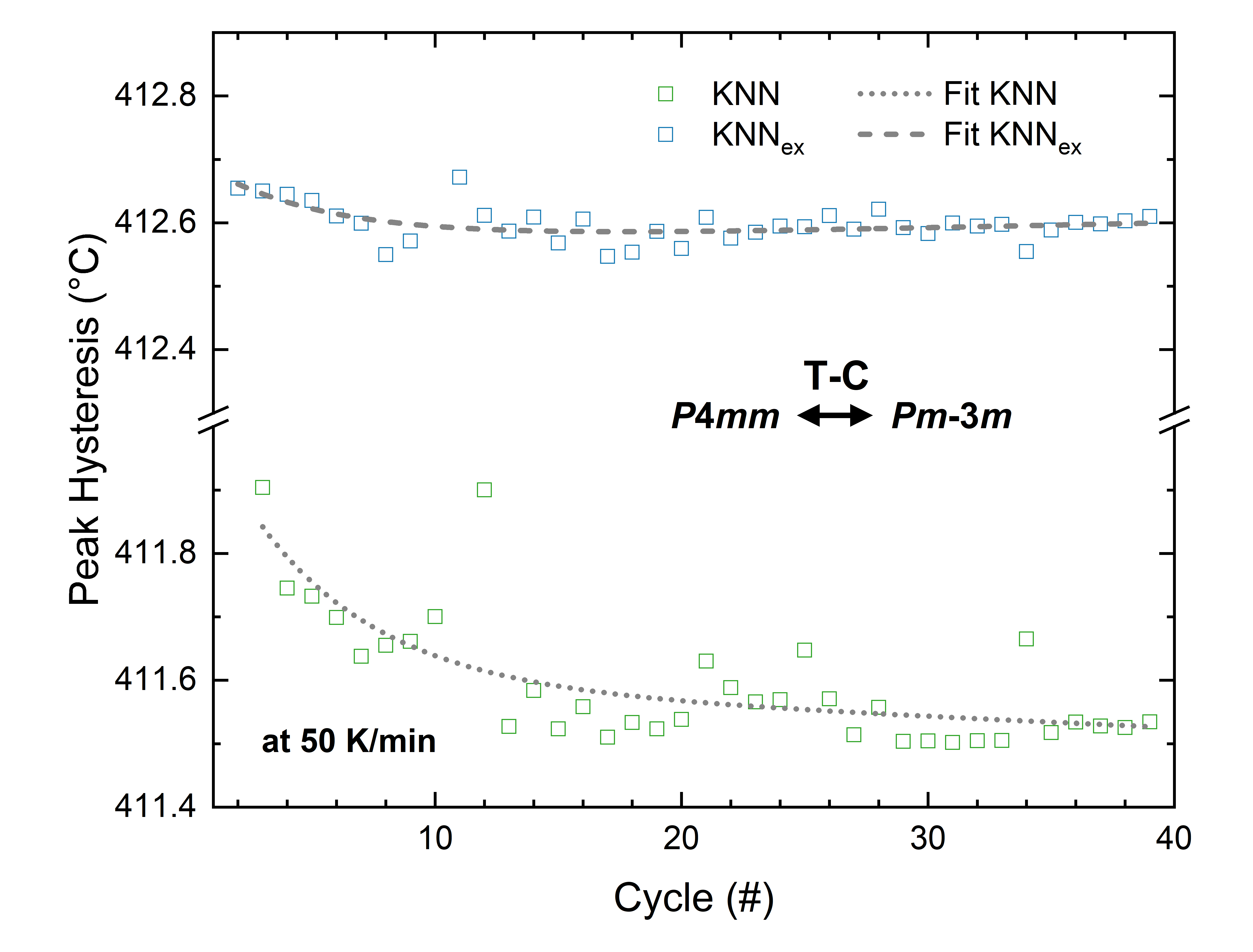
(a)

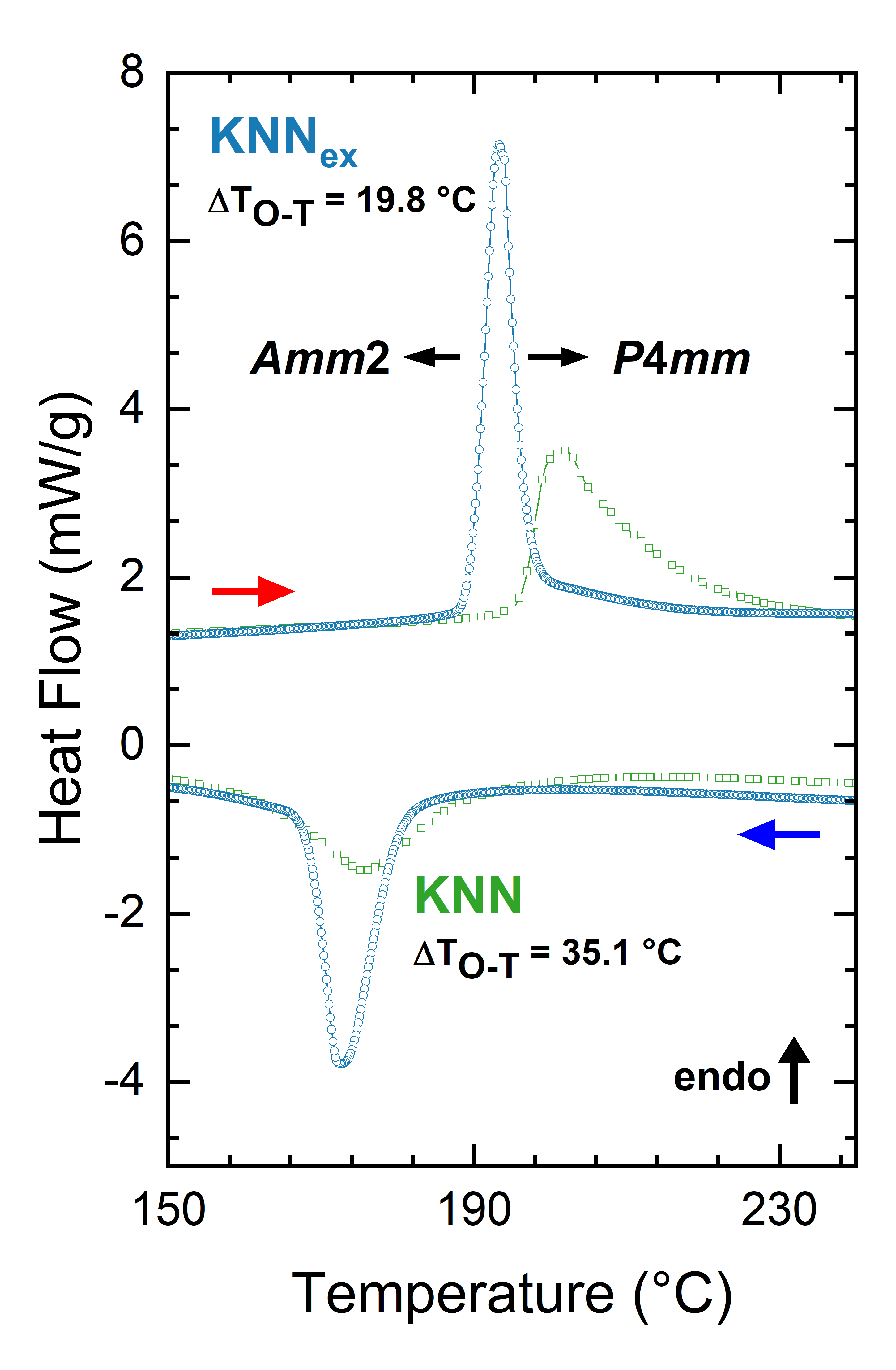
(b)

(c)

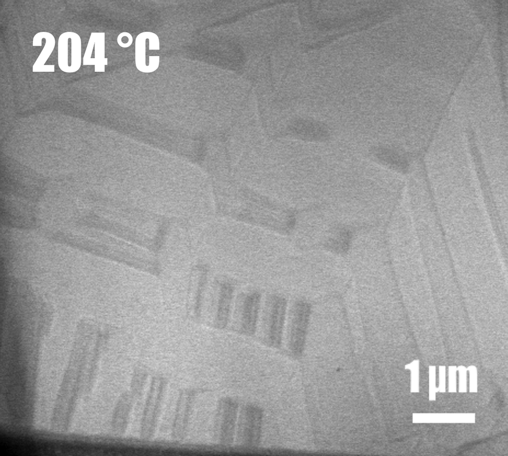
(d)

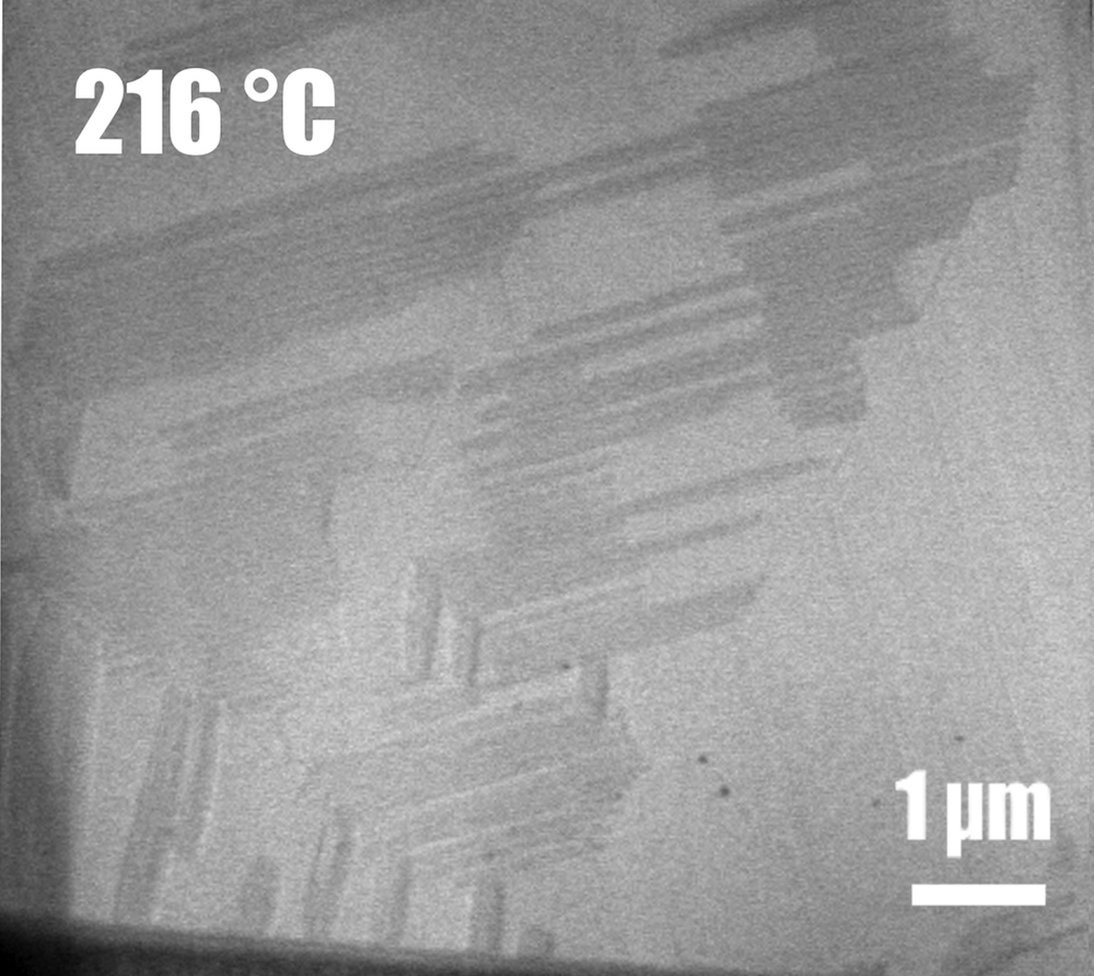
(e)

Figure 1: Upper panel: Differential scanning calorimetry results for LABEL:sub@fig:cycling1: the tetragonal to cubic transition and LABEL:sub@fig:cycling2: the orthorhombic to tetragonal transition in exemplary KNN and KNN_exKNN_ex samples, where $\lambda_{2,KNN}=0.9974$ and $\lambda_{2,KNNex}=0.9977$ respectively. Unit cell schematics and corresponding space groups are given in the insets, respectively. Lower panel: Intermediate twinning as discovered in [1]. Transmission electron microscopy results showing the LABEL:sub@fig:177: pure orthorhombic phase with orthorhombic twinning at 177 °C, LABEL:sub@fig:204: intermediate twinning formed within the orthorhombic variants during the O-T transition and LABEL:sub@fig:216: consumption of the intermediate twins by regular tetragonal variants with completion of the phase transition. Partially adapted from [1].

The presented data shows a clear qualitative difference of temperature variation, where the fatigue-optimized KNN_ex exhibits a significantly tuned phase transition temperature as indicated by the individual two-phase exponential association qualitative fitting functions. In detail, the optimized samples show a standard deviation of $\sigma$ = 0.02872 °C of the T-C transition temperature, while the ordinarily fabricated samples exhibit $\sigma$ = 0.10359 °C, translating to 0.007 % and 0.025 % deviation with regard to the median transition temperatures respectively. Specifically, the first cycles are affected by a training-like effect in KNN, which is essentially neglectable for KNN_ex. Since slower standard heating rates of 10 K $\cdot$ min^-1 were incorporated into these measurements, phase transition temperature shifts are to be seen for the 12th cycle and the 11th cycle for both samples. Each of these is induced by the application of a slower heating rate in the preceding cycle [39]. Taking this into consideration, the phase transition temperature stability is even more pronounced in the fatigue-optimized sample, resulting in standard deviations of 0.06 % (KNN_ex) and 0.31 % (KNN). As for the discovered intermediate twinning state, figure 1b provides details on an exemplary orthorhombic to tetragonal (O-T) transition in KNN_ex, verifying a strong improvement in KNN_ex in terms of sharpness of the transition and amount of released latent heat, which is given by the area under the heat flow signal during the phase transition. From an application perspective, one of the most important improvements is given by the 44 % decrease of hysteresis width from $\Delta T_{KNN}=35.1\>\degree C$ to $\Delta T_{KNNex}=19.8\>\degree C$, with hysteresis width being the main source of loss. Notably, this property improvement is in general more apparent in the O-T transition, exhibiting larger decrease in hysteresis width and significant sharpening of peak shape as compared to 14 % decrease in the T-C transition [1]. Therefore the O-T transition and its intermediate twinning state seem particularly important. Corresponding in-situ transmission electron microscopy results of the O-T transition in KNN_ex demonstrated that the intermediate twinning emerges with the beginning of the phase transition and vanishes completely following the tetragonal to cubic transition. To determine whether the transition path, including the intermediate twinning state, is a consequence of compatibility this experimental data is compared with the proposed model considering energy minimization, as well as depolarization energy. Hence it is worth mentioning that the default directions for spontaneous polarization in the orthorhombic KNN configuration are the $\langle 110\rangle$ directions [19], while in the tetragonal phase the elongation of the unit cell conditions preferred $\langle 100\rangle$ directions for the spontaneous polarization direction [20].

2.2 The electroelastic energy

We employ the nonlinear theory of electrostrictition [22] where in our setting the adopted model is derived directly from the nonlinear theory of magnetostriction [40, 35], by replacing magnetization with polarization. The total energy of the electrostatic configuration is given by

$$E({\bf y},{\bf p},\theta)=\int_{\Omega}W(\nabla{\bf y}({\bf x}),{\bf p}({\bf y}({\bf x})),\theta)d{\bf x}+\frac{1}{2}\int_{\mathbb{R}^{3}}|\nabla_{\bf y}\phi({\bf y})|^{2}d{\bf y},$$ (1)

where ${\bf y}:\Omega\rightarrow\mathbb{R}^{3}$ is the deformation, ${\bf p}:{\bf y}(\Omega)\rightarrow\mathbb{R}^{3}$ is the polarization, $\theta$ denotes the temperature, $W$ is the macroscopic free energy per unit volume and $\phi:{\bf y}(\Omega)\rightarrow\mathbb{R}$ is the electric potential obtained by the unique solution, [41], of the Maxwell’s equation

$$\nabla_{\bf y}\cdot\left(\nabla_{\bf y}\phi({\bf y})+{\bf p}({\bf y})\right)=0,\quad\text{with }\phi({\bf z})\rightarrow 0\text{ as }|{\bf z}|\rightarrow+\infty.$$ (2)

The exchange energy $\nabla{\bf p}\cdot{\bf A}{\bf p}$ with ${\bf A}\in\mathbb{R}^{3\times 3}$ has been neglected in equation (1), under the assumption that domains are much larger than the transition layer between two distinct polarization states [42], giving rise to minimizing sequences [41, 21]. Here the anisotropy energy $W$ models the tendency of the deformations and polarization at the preferred states and $\phi$ is the depolarization field due to the polarization distribution in the material.

In the presented setting the link between the atomistic and the macroscopic deformations is provided by the Cauchy-Born hypothesis where the lattice vectors exhibit locally the same deformation as a macroscopic homogeneous deformation. The validity of the Cauchy-Born hypothesis is ensured by restricting the deformations over a neighborhood of the lattice vectors the Ericksen-Pitteri neighborhood ${\cal N}$, see [31, 32, 27]. Specifically, let the parent lattice $\{{\bf e}_{i}\}\in{\cal N}$, then the produced lattice $\{{\bf F}{\bf e}_{i}\}$ should also belong to the Ericksen-Pitteri neighborhood ${\cal N}$, where ${\bf F}$ is a homogeneous deformation gradient. Additional properties of ${\cal N}$ allow elastic deformations and phase transitions but exclude plastic deformations and slips.

Passing to the continuum scale the anisotropic macroscopic free energy per unit volume $W$ is obtained, where the principles of frame indifference and material symmetry are inherited by the atomistic description of the free energy

$$W({\bf F},{\bf p},\theta) =W({\bf R}{\bf F},{\bf R}{\bf p},\theta),\quad\text{for all }{\bf R}\in SO(3)\text{ (Frane indifference)},$$ (3)

$$W({\bf F},{\bf p},\theta) =W({\bf F}{\bf Q},{\bf p},\theta),\quad\text{for all }{\bf Q}\in{\cal P}({\bf e}_{i})\text{ (Material Symmetry)},$$

here ${\cal P}({\bf e}_{i})$ denotes the point group of the lattice $\{{\bf e}_{i}\}$. Furthermore, it is assumed that there exists a critical temperature $\theta_{c}$ such that the free energy density $W$ is minimized for $({\bf F},{\bf p})=(\mathbf{1},{\bf p}_{1})$, the parent phase, when $\theta\geq\theta_{c}$ and is minimized for $({\bf F},{\bf p})=({\bf U},{\bf p}_{U})$, the produced phase, when $\theta\leq\theta_{c}$. It should be noted if $({\bf U}_{1},{\bf p}_{1})$ is a minimizer of $W$ then due to frame indifference and material symmetry $({\bf R}{\bf U}_{1}\bf Q,{\bf R}{\bf p}_{1})$ is also a minimizer, for all ${\bf R}\in SO(3)$ and ${\bf Q}\in{\cal P}({\bf U}_{1}{\bf e}_{i})$ where $\{{\bf e}_{i}\}$ denotes the parent lattice. The set containing all the minimizers at temperature $\theta$ is defined as

$${\cal M}_{\theta}=\cup_{i=1}^{n}SO(3)\{{\bf U}_{i}(\theta),\pm{\bf p}_{i}(\theta)\},$$ (4)

where ${\bf U}_{i}(\theta)={\bf Q}_{i}^{T}{\bf U}_{1}(\theta){\bf Q}_{i}$, for $i=1,..,n$ and ${\bf Q}_{i}\in{\cal P}({\bf U}_{1}(\theta){\bf e}_{i})$, denote the n distinct variants of the phase at temperature $\theta$. Without loss of generality we assume $W({\bf A},{\bf p}_{A},\theta)=0$ if $({\bf A},{\bf p}_{A})\in{\cal M}_{\theta}$. The energy wells of ${\cal M}_{\theta}$ can be generalized to satisfy the saturation hypothesis $|\det{\bf F}({\bf x}){\bf p}({\bf y}({\bf x}))|=g(\theta)$, [21], for some $g:\mathbb{R}\rightarrow\mathbb{R}^{+}$.

2.3 Minimization of the total energy

Describing the total energy $E({\bf y},{\bf p},\theta)$ from eq. (1) energy minimizing states are studied. Under higher to lower symmetry phase transformations a temperature $\theta_{c}$ exists where the macroscopic free energy $W$ is equi-minimized by the two phases. Coexistance of the phases has been observed in KNN_ex [1]. For the adopted theory, a deformations that minimizes the nonlinear elastic energy $W$ should be $1-1$ and continuous with discontinuous deformation gradient, and the deformation gradient values should belong to the energy wells of ${\cal M}_{\theta}$, eq. (4). Deformations with this property should satisfy the Hadamard jump condition. Specializing the condition, let a region be divided by a plane with normal ${\bf n}$. Deforming the regions, assume the deformation gradient takes the values ${\bf R}{\bf B}\not\in SO(3)$ and ${\bf A}$ on either sides of the planar interface, for some ${\bf R}\in SO(3)$. Then, the deformation ${\bf y}$ is continuous ($\in W^{1,\infty}(\Omega)^{3}$) if and only if the twinning equation

$${\bf R}{\bf B}-\bf{A}={\bf a}\otimes{\bf n},$$ (5)

holds for some ${\bf a}\in\mathbb{R}^{3},a\neq 0$ and $|{\bf n}|=1$, ${\bf a}\otimes{\bf n}$ is a $3\times 3$ matrix with components $({\bf a}\otimes{\bf n})_{ij}=a_{i}n_{j}$, i.e. ${\bf A}$ and ${\bf B}$ must be rank-one connected. Ball and James [26] provided necessary and sufficient conditions for the solution of eq. (5) stating their explicit forms. Specifically, they proved that if the middle eigenvalue of the matrix ${\bf C}={\bf F}^{T}{\bf F}$ is one, where ${\bf F}={\bf B}{\bf A}^{-1}$, then there exists two solutions of (5) denoted by ${\bf R}^{\pm},{\bf a}^{\pm},{\bf n}^{\pm}$. We will call this kind of deformations compatible.

For the same region let ${\bf p}_{A},{\bf p}_{B}$ denote the polarization vectors in the deformed configuration of the phases ${\bf A},{\bf B}$ respectively. The depolarization energy is minimized when $\nabla\phi=\mathbf{0}$, but from eq. (2) this occurs when $\nabla\cdot{\bf p}=0$ for the interior points of the deformed body and when the polarization vector is perpendicular to the normal of $\partial{\bf y}(\Omega)$. Assuming that $\nabla\cdot{\bf p}_{A}=0,\nabla\cdot{\bf p}_{B}=0$ the extra compatibility conditions

$$({\bf p}_{A}-{\bf p}_{B})\cdot{\bf m}=0,\quad\text{where }{\bf m}=\frac{{\bf A}^{-T}{\bf n}}{|{\bf A}^{-T}{\bf n}|}=\frac{{\bf B}^{-T}{\bf n}}{|{\bf B}^{-T}{\bf n}|},$$ (6)

${\bf m}$ is the unit normal of the planar interface in the deformed configuration, ensure divergence free polarization at this plane implying pole-free interfaces, see [21, 22]. When interfaces are formed between different variants of the same phase, these conditions are simplified due to the following lemma:

Lemma 1 (Lemma 6.1 from [21].).

Suppose ${\bf A}$ and ${\bf B}$ are symmetric matrices with $\det{\bf A}=\det{\bf B}$ such that

$${\bf R}{\bf B}-{\bf A}={\bf a}\otimes{\bf n},\text{ for some }{\bf R}\in SO(3),{\bf a},{\bf n}\in\mathbb{R}^{3}.$$ (7)

If ${\bf A}{\bf p}_{A}=\alpha{\bf p}_{A}$ and ${\bf B}{\bf p}_{B}=\alpha{\bf p}_{B}$ for some $\alpha\in\mathbb{R}$, then

$$\left({\bf R}{\bf p}_{B}-{\bf p}_{A}\right)\cdot{\bf m}=0\iff\left({\bf p}_{B}-{\bf p}_{A}\right)\cdot{\bf n}=0,$$ (8)

${\bf m}={\bf A}^{-1}{\bf n}$ is the normal in the deformed configuration.

Based on the compatibility conditions (5) and (8) appropriate deformations and polarization vectors $({\bf y},{\bf p})$, or sequences $({\bf y}_{k},{\bf p}_{k})$, minimizing the total energy will be constructed.

3 Results and Discussion

3.1 Energy minimizing deformations

On the basis of its analogies with martensitic transformations, the phase transitions in KNN_ex can be modeled via sequential energy minimizers of the proposed macroscopic total electroelastic energy, herein potentially predicting the orientation of the interfaces in the orthorhombic phase with high accuracy. In the following, ${\bf e}_{i}$ will denote the lattice vectors defining the unit cell for the cubic phase and polarization is ignored in the first part for simplicity, i.e. it is assumed that ${\bf p}=\bf 0$ in every phase. In martensitic transformations it is common that the martensite phase is not rank-one connected to the higher symmetry austenite phase, which means even if both phases are minimizers there is no continuous deformation satisfying the compatibility conditions (5). Instead the transformation occurs via a more complicated interface known as a classical austenite-martensite interface. Here, a simple laminate between two martensitic variants is formed and a transition layer between the simple laminate and the austenite phase emerges [26, 27, 43, 28, 44]. Let the laminate contain the variants ${\bf U}_{1}$ and ${\bf U}_{2}$ with volume fraction $\lambda$ and $1-\lambda$ respectively, $\lambda\in(0,1)$, the laminate corresponds to the macroscopic deformation gradient

$${\bf A}_{\lambda}=\lambda{\bf R}{\bf U}_{2}+(1-\lambda){\bf U}_{1},\text{ when }{\bf R}{\bf U}_{2}-{\bf U}_{1}={\bf a}\otimes{\bf n}.$$ (9)

Ball and James [26, 27] presented conditions for the existence of laminates between two variants and provided explicit values for $\lambda^{*}$ such that ${\bf A}_{\lambda^{*}}$ and ${\bf A}_{1-\lambda^{*}}$ are rank one connected to $\bf 1$ (the austenite). Then, one can construct a sequence of deformations ${\bf y}_{k}$ in the martensitic region such that as $k\rightarrow+\infty$, ${\bf y}_{k}\buildrel\ast\over{\rightharpoonup}{\bf y}$ in $W^{1,\infty}(\Omega)^{3}$ and ${\bf y}({\bf x})={\bf A}_{\lambda}{\bf x}$, which implies that the energy of the transition layer goes to zero and the macroscopic deformation gradient is ${\bf A}_{\lambda}$, for $\lambda=\lambda*$ or $1-\lambda^{*}$. We show this kind of sequences are also possible for the cubic to tetragonal transition in KNN_ex.

Table 1: Tetragonal variants under cubic to tetragonal transformations.

$$\scriptscriptstyle U_{1}=\begin{pmatrix}\gamma_{t}&0&0\\ 0&\alpha_{t}&0\\ 0&0&\alpha_{t}\end{pmatrix},\quad U_{2}=\begin{pmatrix}\alpha_{t}&0&0\\ 0&\gamma_{t}&0\\ 0&0&\alpha_{t}\end{pmatrix},\quad U_{3}=\begin{pmatrix}\alpha_{t}&0&0\\ 0&\alpha_{t}&0\\ 0&0&\gamma_{t}\end{pmatrix}$$

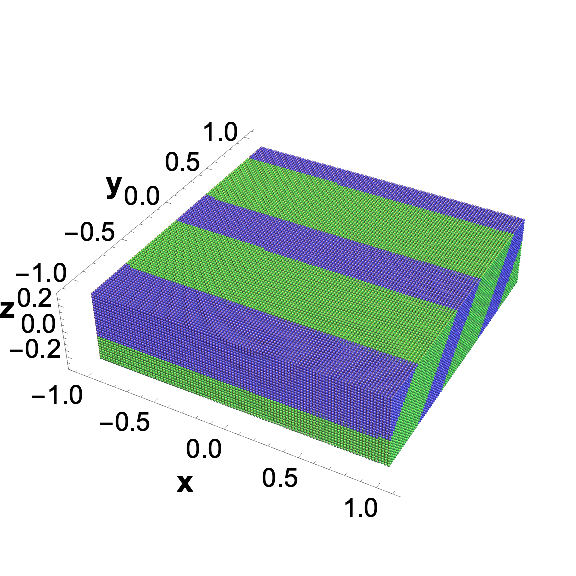
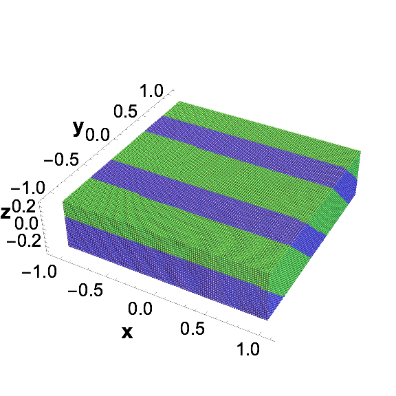
Figure 2: Cubic to tetragonal transformations. Two distinct laminates (green regions) compatible to the cubic phase (blue region). The simple laminate ${\bf A}^{+}_{\lambda}=\lambda{\bf a}^{+}\otimes{\bf n}^{+}+{\bf U}_{1}$ has two interfaces to $\bf{1}$ for $\lambda=\lambda^{*}$ (two figures on the left) and two interfaces for $\lambda=1-\lambda^{*}$ (two figures on the right). $\lambda^{*}\approx 0.335047$. Four different interfaces occur by choosing ${\bf n}^{-}$, see equations (S1), (S4), (S5).

The obtained tetragonal variants are not rank-one connected to the cubic phase using the measured lattice parameters for KNN_ex [1], see table S1 herein. It is implied that the middle eigenvalue $\lambda_{2}\neq 1$, since $\alpha_{t}=3.96/3.98$ and $\gamma_{t}=4.02/3.96$. Instead, the macroscopic deformation (9₁) is compatible to $\bf 1$ due to the conditions specified by Ball and James [26]

$$\alpha_{t}<1<\gamma_{t}\quad\text{and}\quad\frac{1}{\alpha_{t}^{2}}+\frac{1}{\gamma_{t}^{2}}<2.$$ (10)

Figure 2 shows the macroscopically compatible, computed deformation choosing the tetragonal variants ${\bf U}_{1}$ and ${\bf U}_{2}$ from table 1. Therefore, at the Curie temperature there exist a sequence of deformations such that

$$\lim_{k\rightarrow+\infty}E[{\bf y}_{k},\bf{0}]=\lim_{k\rightarrow+\infty}\int_{\Omega}\phi({\bf y}_{k},\bf{0})d{\bf x}=0,$$ (11)

When ${\bf A}_{\lambda}$ is compatible to $\bf 1$ for every $\lambda\in[0,1]$, also known as supercompatibility [45, 46], there is no transition layer, therefore its energy contribution vanishes. This means a wide range of interface angles is energetically preferable facilitating the transformation from one phase to the other. Therefore, supercompatibility conditions, as in the austenite-martensite transitions, is a suggestive mechanism for hysteresis and fatigue reduction in single crystals. Note that for polycrystals extra care is needed, e.g. in [47] irreversibility can occur through the boundary contact of different grains.

In the pure orthorhombic phase (figure 1) more complicated microstructures appear, parallelogram regions meet along a line. We assume these microstructures involve four orthorhombic variants as in the shape memory alloys, where this four fold structure is common and is known as a simple crossing twin or a parallelogram microstructure [40, 43, 48]. Even if the kinematic constraints for the formation of crossing twins are severe we show the microstructure is a consequence of energy minimization through compatible deformations.

Figure 3: The four fold structure formed from a crossing twin in the reference configuration.

Let four distinct orthorhombic variants form a crossing twin (figure 3). From the twinning equation (5) two variants sharing the interface with normal ${\bf n}_{i}$ should be compatible. These rank one-connections do not suffice for a continuous deformations because it should be compatible also at the corners, i.e. the line where the four variants meet. Then, geometric compatibility requires the following

$${\bf R}_{1}{\bf F}_{2}-{\bf F}_{1}={\bf a}_{1}\otimes{\bf n}_{1},\quad{\bf R}_{2}{\bf F}_{3}-{\bf F}_{2}={\bf a}_{2}\otimes{\bf n}_{2}$$ (12)

$${\bf R}_{3}{\bf F}_{4}-{\bf F}_{3}={\bf a}_{3}\otimes{\bf n}_{3},\quad{\bf R}_{4}{\bf F}_{1}-{\bf F}_{4}={\bf a}_{4}\otimes{\bf n}_{4}$$

$${\bf R}_{1}{\bf R}_{2}{\bf R}_{3}{\bf R}_{4}=\bf{1},\text{ with }{\bf R}_{i}\in SO(3),\quad{\bf n}_{1},{\bf n}_{2},{\bf n}_{3},{\bf n}_{4}\text{ coplanar,}$$

where ${\bf R}_{4}=({\bf R}_{1}{\bf R}_{2}{\bf R}_{3})^{T}$. The additional conditions are that the rotations add up to identity and the normal vectors of the interfaces should be coplanar. The former requirement prevents dislocations at the corners while the latter imposes that all four interfaces meet along a line. The majority of the martensitic transformations involve type I and type II twins [28]. These are twins between variants ${\bf A}$ and ${\bf B}$ that are related by a $180\degree$ rotation ${\bf Q}_{\pi}({\bf v})\in{\cal P}({\bf e}_{i})\setminus{\cal P}({\bf A}{\bf e}_{i})$, where ${\bf A}$ is a martensitic variant, ${\bf Q}_{\pi}({\bf v})$ denote $180\degree$ rotation about the axis ${\bf v}$ and ${\bf B}={\bf Q}_{\bf v}(\pi){\bf A}{\bf Q}_{\bf v}(\pi)$. For this type of twins sufficient conditions under which the crossing twins microstructures are compatible have been proved.

Theorem 1 (Theorem 2 in [48]).

Let ${\bf Q}_{1}={\bf Q}_{\pi}({\bf v}_{1})$ and ${\bf Q}_{2}={\bf Q}_{\pi}({\bf v}_{2})$ for ${\bf v}_{1}\cdot{\bf v}_{2}=0$, if

$${\bf F}_{2}={\bf Q}_{1}{\bf F}_{1}{\bf Q}_{1},{\bf F}_{3}={\bf Q}_{2}{\bf F}_{2}{\bf Q}_{2},{\bf F}_{4}={\bf Q}_{2}{\bf F}_{1}{\bf Q}_{2}$$ (13)

then the crossing twins equation (12) has a solution and ${\bf R}_{i},{\bf a}_{i},{\bf n}_{i}$ are given explicitly.

Assuming that type I and type II twins are involved, applying the above theorem we obtain the crossing twin microstructure for cubic to orthorhombic transformations. Let ${\bf V}_{i}$, $i=1,...,6$ denote the orthorhombic variants as shown in table 2. Fixing an orthorhombic variant we would like to find $180\degree$ rotations from the set ${\cal P}({\bf e}_{i})\setminus{\cal P}({\bf V}_{1}{\bf e}_{i})$ such that eq. (13) holds. Setting ${\bf F}_{1}={\bf V}_{5}$, ${\bf Q}_{1}={\bf Q}_{\pi}({\bf e}_{1})$, ${\bf Q}_{2}={\bf Q}_{\pi}({\bf e}_{2}+{\bf e}_{3})$, eq. (13) is satisfied for ${\bf F}_{2}={\bf V}_{6}$, ${\bf F}_{3}={\bf V}_{3}$ and ${\bf F}_{4}={\bf V}_{4}$, ${\bf R}_{i},{\bf a}_{i}$ and ${\bf n}_{i}$ are computed from [48, Theorem 2]. Note that one can choose ${\bf Q}_{1}={\bf Q}_{\pi}({\bf e}_{2}+{\bf e}_{3})$, ${\bf Q}_{2}={\bf Q}_{\pi}({\bf e}_{1})$ resulting in a different crossing twin. We have chosen the former rotations due to better agreemet with experiments. Let $\Omega$ describe the cubic phase (reference configuration), we define the deformation ${\bf y}({\bf x})={\bf B}({\bf x}){\bf x}$, ${\bf x}\in\Omega$, where

$${\bf B}(x)=\begin{cases}{\bf V}_{5},&\text{if }{\bf x}\cdot{\bf n}_{1}\geq 0\text{ and }{\bf x}\cdot{\bf n}_{4}<0,\\ {\bf R}_{1}{\bf V}_{6},&\text{if }{\bf x}\cdot{\bf n}_{2}\geq 0\text{ and }{\bf x}\cdot{\bf n}_{1}<0,\\ {\bf R}_{1}{\bf R}_{2}{\bf V}_{3},&\text{if }{\bf x}\cdot{\bf n}_{3}\geq 0\text{ and }{\bf x}\cdot{\bf n}_{2}<0,\\ {\bf R}_{1}{\bf R}_{2}{\bf R}_{3}{\bf V}_{4},&\text{if }{\bf x}\cdot{\bf n}_{4}\geq 0\text{ and }{\bf x}\cdot{\bf n}_{3}<0.\end{cases}$$ (14)

For this deformation the twins with interfaces between ${\bf V}_{5},{\bf V}_{6}$ and ${\bf V}_{3},{\bf V}_{4}$ are compound twins and for interfaces between ${\bf V}_{4},{\bf V}_{5}$ and ${\bf V}_{3},{\bf V}_{6}$ are of type $II$, see also [48]. Deformation ${\bf y}$ is continuous, piecewise homogeneous and minimizes the elastic energy i.e. $(\nabla{\bf y},\bf{0})\in{\cal M}_{\theta_{o}}$, $\theta_{o}=187\degree$ (orthorhombic phase in figure 1). In figures 4a and 4b the reference state (cubic) and the deformed configuration of orthorhombic crossing twins are illustrated. More complicated microstructures are formed in figure 4c(S1a) and extended through isometry groups (SM:Extending energy minimizing deformations), figure 4d(S1b), [49, 50]. Here the reference configuration and the deformation are extended using a translation along the direction ${\bf n}_{1}$ and repeating the procedure a second extension is performed along direction $({\bf n}_{1}\times{\bf n}_{2})\times{\bf n}_{1}$. The most striking feature of this model concerns the angles formed between the interfaces of the crossing twins. Images obtained from scanning transmission electron microscopy (STEM) artificially colored emphasize the interfaces between the orthorhombic variants. Plotting the theoretical predicted interfaces a great agreement between theory and experiment is observed (figure 5). Here we should comment that we modeled the narrow bands of figure 5a as alternating orthorhombic variants. These narrow bands can also indicate the formation of $180\degree$ domains, as it will be shown in the sequel that these domains minimize the electrostatic energy in the interior of the body. Therefore, we propose two distinct underlying mechanism for the formation of narrow bands which in the presence of small strains are indistinguishable and both minimize the total electroelastic energy. One can ask which one of the two phenomena appears? The requirement of the very restrictive state, the set of compatibility conditions (12), during the formation of the crossing twins proposes that $180\degree$ domains are most likely present.

Table 2: Orthorhombic variants under cubic to orthorhombic transformations.

$$V_{1}=\begin{pmatrix}\gamma_{o}&0&0\\ 0&\frac{\alpha_{o}+\beta_{o}}{2}&\frac{\alpha_{o}-\beta_{o}}{2}\\ 0&\frac{\alpha_{o}-\beta_{o}}{2}&\frac{\alpha_{o}+\beta_{o}}{2}\end{pmatrix},V_{2}=\begin{pmatrix}\gamma_{o}&0&0\\ 0&\frac{\alpha_{o}+\beta_{o}}{2}&\frac{\beta_{o}-\alpha_{o}}{2}\\ 0&\frac{\beta_{o}-\alpha_{o}}{2}&\frac{\alpha_{o}+\beta_{o}}{2}\end{pmatrix},V_{3}=\begin{pmatrix}\frac{\alpha_{o}+\beta_{o}}{2}&0&\frac{\alpha_{o}-\beta_{o}}{2}\\ 0&\gamma_{o}&0\\ \frac{\alpha_{o}-\beta_{o}}{2}&0&\frac{\alpha_{o}+\beta_{o}}{2}\end{pmatrix}$$

$$V_{4}=\begin{pmatrix}\frac{\alpha_{o}+\beta_{o}}{2}&0&\frac{\beta_{o}-\alpha_{o}}{2}\\ 0&\gamma_{o}&0\\ \frac{\beta_{o}-\alpha_{o}}{2}&0&\frac{\alpha_{o}+\beta_{o}}{2}\end{pmatrix},V_{5}=\begin{pmatrix}\frac{\alpha_{o}+\beta_{o}}{2}&\frac{\beta_{o}-\alpha_{o}}{2}&0\\ \frac{\beta_{o}-\alpha_{o}}{2}&\frac{\alpha_{o}+\beta_{o}}{2}&0\\ 0&0&\gamma_{o}\end{pmatrix},V_{6}=\begin{pmatrix}\frac{\alpha_{o}+\beta_{o}}{2}&\frac{\beta_{o}-\alpha_{o}}{2}&0\\ \frac{\beta_{o}-\alpha_{o}}{2}&\frac{\alpha_{o}+\beta_{o}}{2}&0\\ 0&0&\gamma_{o}\end{pmatrix}$$

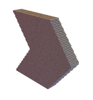
(a)

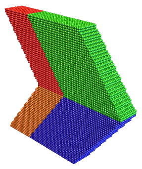
(b)

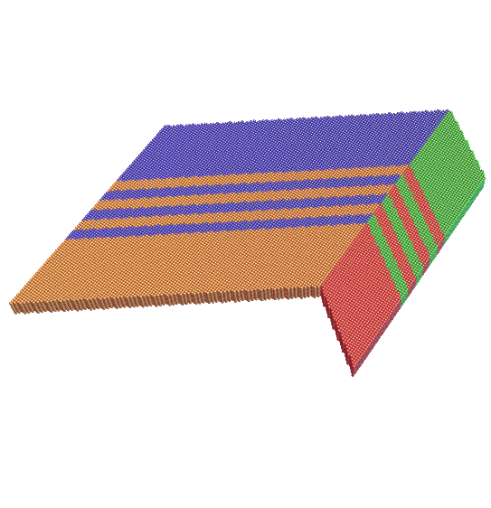
(c)

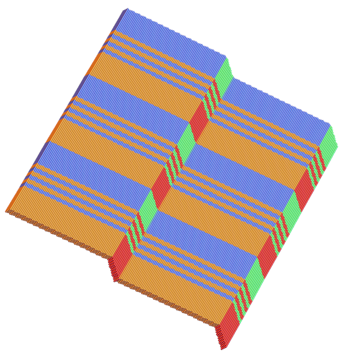
(d)

Figure 4: Formation of orthorhombic crossing twins. LABEL:sub@fig:orthorhombic_ref: Cubic reference configuration. LABEL:sub@fig:orthorhombic_def: Orthorhombic deformed configuration. The variants ${\bf V}_{3},{\bf V}_{4},{\bf V}_{5}$ and ${\bf V}_{6}$ correspond to orange, red, green and blue coloring respectively. Consequently, the orthorhombic crossing twins in the C-T transition can be constructed. First, the microstructure of LABEL:sub@fig:orthorhombic_def2: is created and subsequently extended through isometry groups in LABEL:sub@fig:orthorhombic_def2_ext.

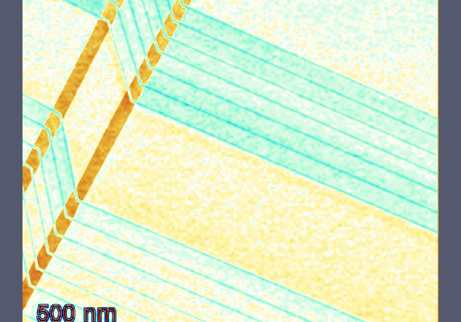
(a)

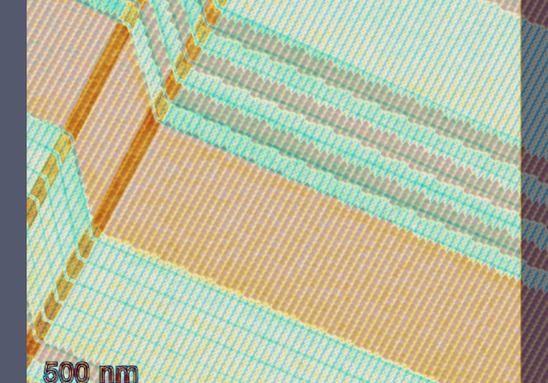
(b)

Figure 5: Comparing experimental observed and theoretical predicted interfaces between orthorhombic variants. LABEL:sub@fig:exp_crossing_bands :Artificial colored STEM image of the orthorhombic phase distinguishing different orthorhombic variants, reproduced from [1]. LABEL:sub@fig:crossing_bandscomp: Experimental image is superposed with the theoretical computed crossing twin from Figure 4c. The theoretical interfaces coincide with the experimental observation.

It remains to examine why the intermediate twinning between orthorhombic and tetragonal phase emerge, figure 1, where tetragonal twins grow within an orthorhombic variant. If a laminate between two tetragonan variants is compatible to the initial orthorhombic phase then intermediate twinning is energetically favorable according to the adopted theory. Choosing the tetragonal variants ${\bf U}_{1},{\bf U}_{2}$ (table 1), solutions of the twinning equations

$${\bf Q}{\bf A}^{\pm}_{\mu}-{\bf V}_{i}={\bf b}_{i}\otimes{\bf m}_{i},\text{ }i=1,...,6\text{ for some }\mu\in[0,1],$$ (15)

$$\text{where}\quad{\bf A}^{\pm}_{\mu}=\mu{\bf R}^{\pm}{\bf U}_{2}+(1-\mu){\bf U}_{1}=\mu{\bf a}^{\pm}\otimes{\bf n}^{\pm}+{\bf U}_{1},$$ (16)

are examined (${\bf a}^{\pm},{\bf n}^{\pm}$ are provided by eqs. (S1) ). Solutions of eq. (15) exist when the middle eigenvalue of ${\bf C}_{i,\mu}^{\pm}=\left({\bf F}_{i,\mu}^{\pm}\right)^{T}{\bf F}_{i,\mu}^{\pm}$ is $1$, where ${\bf F}_{i,\mu}^{\pm}={\bf A}^{\pm}_{\mu}{\bf V}_{i}^{-1}$. Plotting the eigenvalues of ${\bf C}_{i,\mu}^{+}$ (${\bf C}_{i,\mu}^{-}$) in figure 6 (S2), it is shown that there exists at least one value of $\mu$ such that the laminate between ${\bf U}_{1}$ and ${\bf U}_{2}$ is compatible with every orthorhombic variant. At the transition temperature $\theta_{OT}=202\degree$, the set of minimizers is ${\cal M}_{\theta_{OT}}=\left(\cup_{k=1}^{6}SO(3)\{{\bf V}_{k},\bf{0}\}\right)\cup\left(\cup_{i=1}^{3}SO(3)\{{\bf U}_{i},\bf{0}\}\right),$ which means for every orthorhombic variant there exists sequences of deformations ${\bf y}_{k}$ involving tetragonal variants such that the total potential energy is minimized as $k\rightarrow+\infty$. Therefore, the formation of intermediate twinning can be interpreted as an energetically preferred state.

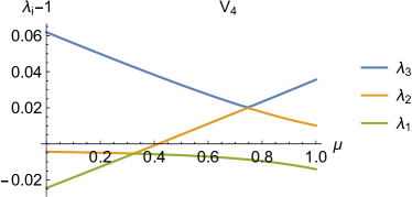
Figure 6: Eigenvalues $\lambda_{i}$ of ${\bf C}_{i,\mu}^{+}$ over volume fraction $\mu$ of a laminate between the tatragonal variants ${\bf U}_{1},{\bf U}_{2}$. Let $\mu^{*}$ be the fraction such that $\lambda_{1}\leq\lambda_{2}=1\leq\lambda_{3}$, then the laminate with volume fraction $\mu^{*}$ is compatible with the orthorhombic variant ${\bf V}_{i}$.

3.2 Incorporating polarization in energy minimization

In the adopted nonlinear theory of electrostrictition domains are identified as energy minimizing states, [22]. In this nonlinear theory these states are based on compatibility conditions that minimize the depolarization energy, as in the development of magnetic domains presented in [21, 35]. In the greater number of cases in ferromagnetism easy axes are related to the eigenvectors (stretch directions) of the martensite variants, [35]. In the following it is assumed that polarization emerge along stretch directions. According to [19] default directions for spontaneous polarization in the orthorhombic KNN configuration are the $\langle 110\rangle_{c}$. These equivalent crystallographic directions correspond to the eigenvectors with eigenvalues $\alpha_{o}$ and $\beta_{o}$ for every orthorhombic variant ${\bf V}_{i}$ (table 2). For KNN_ex, $\alpha_{o}\simeq 0.9899$ and $\beta_{o}\simeq 1.002$. Let us choose $\beta_{o}$, the justification for this preference is left for later. From the aforementioned observations it is natural to assume that ${\bf p}_{5}=p_{s}\hat{{\bf p}}_{5}$, where $\hat{{\bf p}}_{5}=\frac{-{\bf e}_{1}+{\bf e}_{2}}{\sqrt{2}}$, for the energy well $SO(3)\{{\bf V}_{5},\pm{\bf p}_{5}\}$. Every orthorhombic variant ${\bf V}_{i}$ can be obtained through the relation ${\bf V}_{i}={\bf R}_{i}{\bf V}_{5}{\bf R}_{i}^{T}$, ${\bf R}_{i}\in{\cal P}({\bf V}_{5}{\bf e}_{i})$. Together with ${\bf V}_{5}{\bf p}_{5}=\beta_{o}{\bf p}_{5}$ it is deduced that ${\bf p}_{i}={\bf R}_{i}{\bf p}_{5}$ and ${\bf V}_{i}{\bf p}_{i}=\beta_{0}{\bf p}_{i}$. Consequently, our assumption that polarization occurs along the direction with stretch $\beta_{0}$ is consistent for every variant. For convenience, the unit polarization vectors for the variants ${\bf V}_{5},{\bf V}_{6},{\bf V}_{3}$ and ${\bf V}_{4}$ involved in the crossing twin of figure 4, are given explicitly

$$\hat{{\bf p}}_{5}=\frac{-{\bf e}_{1}+{\bf e}_{2}}{\sqrt{2}},\text{ }\hat{{\bf p}}_{6}=\frac{{\bf e}_{1}+{\bf e}_{2}}{\sqrt{2}},\text{ }\hat{{\bf p}}_{3}=\frac{-{\bf e}_{1}+{\bf e}_{3}}{\sqrt{2}},\text{ }\hat{{\bf p}}_{4}=\frac{{\bf e}_{1}+{\bf e}_{3}}{\sqrt{2}}.$$ (17)

Here it is implied ${\bf p}_{i}=p_{s}\hat{{\bf p}}_{i}$, where $p_{s}$ accounts for saturation. In the orthorhombic phase, $\theta_{o}=187\degree$, energy wells are described by the set ${\cal M}_{\theta_{o}}=$$\cup_{i=1}^{6}SO(3)\{{\bf V}_{i},$ $\pm{\bf p}_{i}\}$. Not let $\{\nabla{\bf y}({\bf x}),{\bf p}({\bf x})\}\in{\cal M}_{\theta_{o}}$ for all ${\bf x}\in\Omega$, $\Omega$ is the reference configuration (cubic state). Then under the formation of the crossing twin, the only contribution to the total energy of the electrostatic configuration is due to the depolarization energy, specifically the total energy is

$$E[{\bf y},{\bf p},\theta]=\frac{1}{2}\int_{\mathbb{R}^{3}}|\nabla\phi({\bf z})|^{2}d{\bf z}.$$ (18)

The depolarization energy vanishes when $\Div{\bf p}=0$, and it is divergence free if the polarization jump conditions (eq. (8)) are satisfied at the interfaces between the variants. Surprisingly, choosing sings with order $\pm{\bf p}_{5},\mp{\bf p}_{6},\pm{\bf p}_{3},\mp{\bf p}_{4}$, condition (8) holds. Hence, depolarization energy is minimized in the interior of the body. To validate this observation one needs to notice first that the specific deformation of eq. (14) implies

$${\bf n}_{1}=-{\bf n}_{3}={\bf e}_{1},\text{ }{\bf n}_{4}\cdot{\bf e}_{3}={\bf n}_{2}\cdot{\bf e}_{2},\text{ }{\bf n}_{4}\cdot{\bf e}_{2}={\bf n}_{2}\cdot{\bf e}_{3},\text{ }{\bf n}_{2}\cdot{\bf e}_{3}=-{\bf n}_{2}\cdot{\bf e}_{2},$$ (19)

where conditions (12) hold for every ${\bf n}_{i}$. Then for every interface between two orthorhombic variants condition (8) is satisfied, namely

$$({\bf p}_{5}+{\bf p}_{6})\cdot{\bf n}_{1}=({\bf p}_{6}+{\bf p}_{3})\cdot{\bf n}_{2}=({\bf p}_{3}+{\bf p}_{4})\cdot{\bf n}_{3}=({\bf p}_{4}+{\bf p}_{5})\cdot{\bf n}_{4}=0.$$ (20)

Note that the above equations do not imply that depolarization energy is zero due to possible contributions of $\Div{\bf p}_{i}$ at the boundary of the grain.

Now let the narrow bands in figure 5a represent $180\degree$ domains within a variant, for example the crossing twin microstructure with their respective polarization vectors are illustrated in figure 7. But why are these $180\degree$ domains energetically preferable? First, one can notice that $\Div{\bf p}=0$ still holds in the interior of each variant, i.e. there is no contribution to the depolarization energy from the bulk. Furthermore, the formation of these domains can be considered as a part of a sequence minimizing the total energy. For simplicity, assume the homogeneous deformations ${\bf y}({\bf x})={\bf F}{\bf x}$ is performed on $\Omega$ and let $\{{\bf F},\pm{\bf p}\}\in{\cal M}_{\theta}$. Let ${\bf m}$ be normal to ${\bf p}$ with $|{\bf m}|=1$ and ${\bf p}_{k}$ the sequence depicted in figure 8. It has been shown, [21, Proposition 5.1], that as $k\rightarrow\infty$ the depolarization energy goes to zeros. This can be considered as a macroscopic zero polarization that cancels energy contributions from the boundary. This is a possible mechanics for domains formation of this kind and suggests that different geometries should affect domains structure. We must note that these structures are not predicted choosing eigenvectors that correspond to the eigenvalue $\alpha_{o}$.

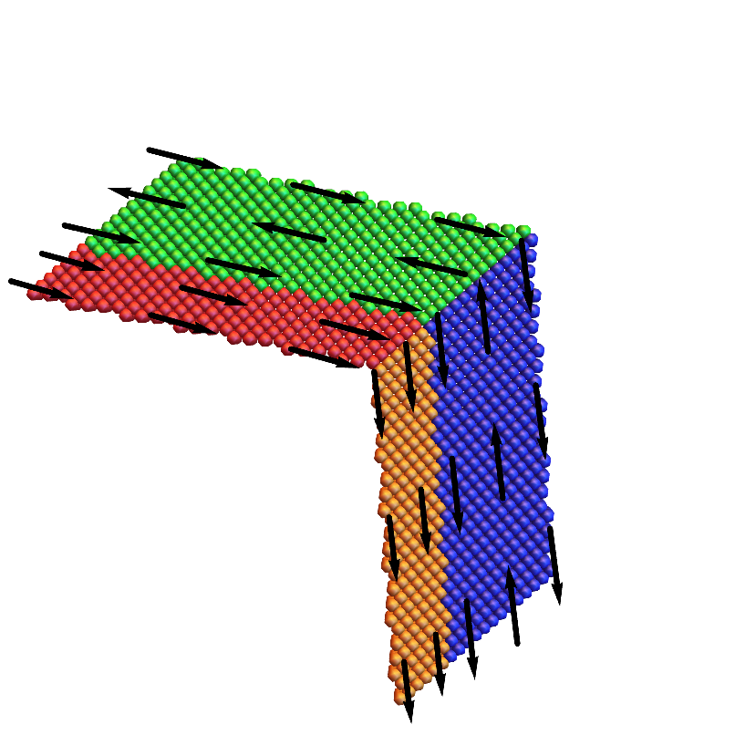
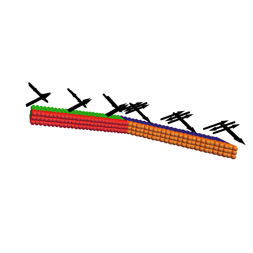
Figure 7: Different angles of spontaneous polarization in top of variants ${\bf V}_{5}$, ${\bf V}_{6}$, ${\bf V}_{3}$ and ${\bf V}_{4}$ (green, blue, orange and red). Here $180\degree$ domains are formed within ${\bf V}_{5}$ and ${\bf V}_{6}$ variants, proposing an underlying mechanics for the formations of the observed narrow bands of figure 5a. We have chosen the compatible polarizaion vectors ${\bf p}_{5}=p_{s}\hat{{\bf p}}_{5}$, ${\bf p}_{6}=-p_{s}\hat{{\bf p}}_{6}$, ${\bf p}_{3}=p_{s}\hat{{\bf p}}_{3}$ and ${\bf p}_{4}=-p_{s}\hat{{\bf p}}_{4}$, $\hat{{\bf p}}_{i}$ is given from equation (17).

Figure 8: A sequence ${\bf p}_{k}$ forming $180\degree$ domains along ${\bf m}$, where ${\bf m}$ is normal to the polarization vector ${\bf p}$. The region is subdivided into $2k$ subregions representing domains.

In the tetragonal phase the elongation of the unit cell conditions preferred $\langle 100\rangle_{c}$ directions for the spontaneous polarization direction [20]. Then each tetragonal variant is related by the polarization direction through

$${\bf U}_{i}=\alpha_{t}\mathbf{1}+(\gamma_{t}-\alpha_{t})\hat{{\bf p}}_{i}\otimes\hat{{\bf p}}_{i},\quad\text{where }\hat{{\bf p}}_{i}={\bf e}_{i}\quad\text{and }{\bf p}_{i}=p_{s}\hat{{\bf p}}_{i}.$$ (21)

For the measured lattice parameters (table S1) two distinct tetragonal variants are rank-one connected. In pure tetragonal phase the energy wells are described by ${\cal M}_{\theta_{T}}=\cup_{i=1}^{3}SO(3)\{{\bf U}_{i},\pm{\bf p}_{i}\}$. As before, if ${\bf U}_{j}={\bf R}{\bf U}_{k}{\bf R}^{T}$ then ${\bf p}_{j}={\bf R}{\bf p}_{k}$, ${\bf R}\in{\cal P}({\bf U}_{k}{\bf e}_{i})$ and condition (8) is satisfied. For instance take the twin formed from ${\bf U}_{1}$ and ${\bf U}_{2}$. The two possible interfaces have normals ${\bf n}^{\pm}=(1,\pm 1,0)$, resulting to $({\bf p}_{2}-{\bf p}_{1})\cdot{\bf n}^{+}=0$ and $({\bf p}_{2}+{\bf p}_{1})\cdot{\bf n}^{-}=0$, which implies there is no depolarization energy in the interior of the twin. Then, following the proof of [21, Theorem5.2] there exists a minimizing sequence $\{{\bf y}_{k},{\bf p}^{k}\}$ such that the total electroelastic energy is minimized as $k\rightarrow+\infty$. A sequence with these properties can be seen in [21, Figure 1], which is a sequence of $180\degree$ domains within each tetragonal variant appearing similar to the aforementioned orthorhombic case, figure 7. Similarly for any other choice of two tetragonal variants. Therefore, the experimentaly observed directions of spontaneous polarization in both the orthorhombic and tetragonal phase, [19, 20], can be interpreted as energy minimizing directions through the adopted nonlinear setting. In the absence of any other comparable experimental data we avoid to present more details about these sequences.

4 Conclusion

Within this work, we employ a full nonlinear electroelastic energy for modeling the recently observed intermediate twinning, first order phase transitions and spontaneous polarization in KNN_ex. The nonlinear theory has been developed in the framework of electrostricion and geometrically nonlinear elasticity. We shown that cubic to tetragonal and tetragonal to orthorhombic phase transitions are energetically favorable through minimizing sequences $\{{\bf y}_{k}\}$, where the total potential energy is minimized as $k\rightarrow+\infty$. These sequences correspond to simple or complex laminates among variants of the involved phase and $k\rightarrow+\infty$ represents fine phase mixtures. Intermediate twinning is interpreted as a laminate of this type, but departing from common practice, the laminate contains the higher symmetry tetragonal variants and it is compatible to a lower symmetry orthorhombic variant. The most striking agreement between theory and experiments occurs in the pure orthorhombic phase where crossing twins arise. Four interfaces separating four distinct orthorhombic variants intersect along a line. The agreement between theoretical predicted and experimentally observed angles is remarkable. With respect to the spontaneous polarization assuming that the polarization directions coincide with a stretch directions of the correlated phase the depolarization energy is minimized. Despite complex stoichiometries and transition paths in KNN_ex, the phase transition and domain dynamics obey energy minimization at all times and can thus be manipulated along the set of presented criteria. We believe that the nonlinear electroelastic theory can serve as a powerful tool in understanding, exploring and tailoring the electromechanical properties of complex ferroelectric ceramics.

Materials and methods

The $K_{0.5}Na_{0.5}NbO_{3}$ (KNN) and KNN plus excess alkali metals (KNNex) bulk samples providing the basis for the applied model have been fabricated by solid-state route, where the detailed procedure is available elsewhere [38]. In specific, KNNex samples exhibit homogeneous grain growth and have thus been chosen for comparison of the experimental results with the developed model. KNNex describes samples fabricated along improved process parameters yielding suppressed abnormal grain growth and fatigue optimization with the criteria of compatibility, since the suppression of multi-scale heterogeneities allows for the accurate application of a model. Herein, KNNex describes $K_{0.5}Na_{0.5}NbO_{3}$ samples with an alkali metal (A-site) excess of 5 mole-% potassium and 15 mole-% sodium in comparison to conventional equimolar KNN samples without any intentional deviation on the A-site. The first set of data was measured with a NETZSCH DSC 204 F1 Phoenix differential scanning calorimeter (DSC), the second set was measured with a TA Instruments Q1000. Samples were cycled at a standard rate of 10 K $\cdot$ min¹ for the first and second cycle, as well as at elevated degeneration conditions of 50 K $\cdot$ min¹ for the following cycles. The tangent method was used for the determination of the thermal hysteresis $\Delta T$ using the equation $\Delta T=1/2((A_{s}+A_{f})-(M_{s}+M_{f}))$. Herein, $A_{s},A_{f},M_{s}$ and $M_{f}$ represent the respective austenitic (high-symmetry) and martensitic (low-symmetry) start and finish temperatures. With regard to reproducibility the stability of the experimental DSC parameters is verified in a preceding experiment, particularly for the heating cycle. The detailed transmission electron microscopy (TEM) results are part of a different experiment [1], and serve as an experimental verification to the developed model.

Funding

This work’s support by a Vannevar Fellowship is gratefully acknowledged.

Declaration of competing interest

The authors declare that they have no known competing financial interests or personal relationships that could have appeared to influence the work reported in this paper.

Data availability

The data that support the findings of this study are available from the corresponding author upon reasonable request.

5 Supplementary material

5.1 Cubic to tetragonal transformations

A compatible laminate (between two tetragonal variants) to the cubic phase is constructed. We have chosen ${\bf U}_{1}$ and ${\bf U}_{2}$ from table 1 as the tetragonal variants contained in the simple laminate ${\bf A}_{\lambda}$. The twinning equation ${\bf R}{\bf U}_{2}-{\bf U}_{1}$ is solved through [26, Proposition 4], which has the solutions $({\bf R}^{+},{\bf a}^{+},{\bf n}^{+})$ and $({\bf R}^{-},{\bf a}^{-},{\bf n}^{-})$, where

$${\bf n}^{\pm}=\frac{1}{\sqrt{2}}(1,\pm 1,0),\quad{\bf a}^{\pm}=\frac{\sqrt{2}(a_{t}-c_{t})}{a_{t}^{2}+c_{t}^{2}}(\pm c_{t},a_{t},0),$$ (S1)

Note that ${\bf R}^{\pm}=\left({\bf U}_{1}+{\bf a}^{\pm}\otimes{\bf n}^{\pm}\right){\bf U}_{2}^{-1}$. The laminates

$${\bf A}_{\lambda}^{\pm}=\lambda{\bf R}^{\pm}{\bf U}_{2}+(1-\lambda){\bf U}_{1}$$ (S2)

are compatible to the cubic phase, see [26], for $\lambda=\lambda^{*}$ or $\lambda=1-\lambda*$ where

$$\lambda^{*}=\frac{1}{2}\left(1-\sqrt{1+\frac{2}{\delta^{\pm}}}\right),\quad\text{and}\quad\delta^{\pm}={\bf a}^{\pm}\cdot{\bf U}_{1}({\bf U}_{1}-\bf{1})^{-1}{\bf n}^{\pm}.$$ (S3)

Note there are four solutions resulting from the combinations

$$({\bf R}^{+},{\bf a}^{+},{\bf n}^{+},\lambda^{*}),\quad({\bf R}^{+},{\bf a}^{+},{\bf n}^{+},1-\lambda^{*}),$$ (S4)

$$({\bf R}^{-},{\bf a}^{-},{\bf n}^{-},\lambda^{*}),\quad({\bf R}^{-},{\bf a}^{-},{\bf n}^{-},1-\lambda^{*}).$$

A choice from (S4), e.g. take ${\bf A}_{\lambda^{*}}^{\pm}$ solves

$${\bf R}_{i}{\bf A}_{\lambda^{*}}^{\pm}-\mathbf{1}={\bf b}_{i}\otimes{\bf m}_{i},\quad i=1\text{ or }2,$$ (S5)

which has two solutions, which means there are $8$ possible laminates between ${\bf U}_{1}$ and ${\bf U}_{2}$ compatible with the cubic phase. Including also ${\bf U}_{3}$, there are overall 24 possible cubic to tetragonal interfaces. For figure 2 we have chosen the laminate produced from $({\bf R}^{+},{\bf a}^{+},{\bf n}^{+},\lambda^{*})$.

5.2 Extending energy minimizing deformations

Here given a zero energy deformation ${\bf y}$ defined on $\Omega$, we extend both the domain $\Omega$ and the deformations ${\bf y}$ in a way such that the total energy for the extended deformation remains zero (minimum). We follow the method of objective structures [49, 50], an example is the isometry group where elements of orthogonal transformations with translations are employed. The elements belong to the set $\{({\bf R}|{\bf c})\}$, for ${\bf R}\in O(3)$ and ${\bf c}\in\mathbb{R}^{3}$. If this set is equipped with the composition $({\bf R}_{1}|{\bf c}_{1})({\bf R}_{2}|{\bf c}_{2})=({\bf R}_{1}{\bf R}_{2}|{\bf c}_{1}+{\bf R}_{1}{\bf c}_{2})$, the identity $(\bf I,0)$ and the inverse of $({\bf R}|{\bf c})$ to be $({\bf R}^{T},-{\bf R}^{T}{\bf c})$ then isometries form a group. For our examples, the reference configuration is extended from $\Omega$ to $\Omega_{E}$ through the translation $t({\bf x})={\bf x}+{\bf w}$, ${\bf w}$ is the translation vector and $|{\bf w}|$ equals the the width of $\Omega$ along the translation direction. The extended domain is

$$\Omega_{E}=\cup_{i=0}^{n}t^{i}(\Omega),\text{ where }t^{k}({\bf x})=t(t(\dots\text{k-times}({\bf x})\dots)).$$ (S6)

Similartly, from the second isometry $h({\bf x})={\bf x}+{\bf c}$ the definition of ${\bf y}:\Omega\rightarrow\mathbb{R}^{3}$ it is extended to $\Omega_{E}$ through

$${\bf y}_{E}({\bf x})=h^{i}\left({\bf y}\left(t^{-i}({\bf x})\right)\right),\text{ for all }{\bf x}\in t^{-i}({\bf x})\Rightarrow\text{ for all }{\bf x}\in\Omega_{E},$$ (S7)

where ${\bf c}$ ensures the continuity of the deformations. If ${\bf y}$ is a zero energy deformation in $\Omega$ then ${\bf y}_{E}$ will be a zero energy deformation in $\Omega_{E}$ because the free energy function $\phi$ is invariant under translations.

Table S1: Lattice parameters from X-ray diffraction measurements for KNN_ex [1]. Distance unit: Å.

Orthorhombic	Tetragonal	Cubic
$a_{o}=3.94$	$a_{t}=3.96$	$a_{c}=3.98$
$b_{o}=5.64$
$c_{0}=5.67$	$c_{t}=4.02$

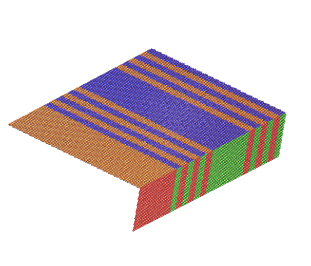
(a)

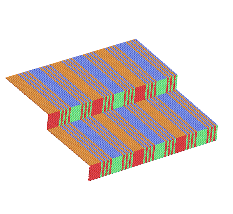
(b)

Figure S1: The orthorhombic crossing twin under cubic to orthorhombic transformation is constructed. variants ${\bf V}_{3},{\bf V}_{4},{\bf V}_{5}$ and ${\bf V}_{6}$ correspond to orange, red, green and blue colors. First microstructure of LABEL:sub@fig:orthorhombic_def3 is created and is extended through isometry groups to LABEL:sub@fig:orthorhombic_def3_ext.

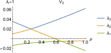
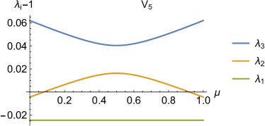
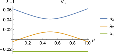
Figure S2: Eigenvalues $\lambda_{i}$ of ${\bf C}_{i,\mu}^{-}$ over volume fraction $\mu$ of a laminate between the tatragonal variants ${\bf U}_{1},{\bf U}_{2}$. Let $\mu^{*}$ be the fraction such that $\lambda_{1}\leq\lambda_{2}=1\leq\lambda_{3}$, then the laminate with volume fraction $\mu^{*}$ is compatible with the orthorhombic variant ${\bf V}_{i}$.

References

-
[1]
P. Pop-Ghe, M. Amundsen, C. Zamponi, A. Gunnæs, E. Quandt,
Direct observation of
intermediate twinning in the phase transformations of ferroelectric potassium
sodium niobate, Ceramics International 47 (14) (2021) 20579–20585.
doi:10.1016/j.ceramint.2021.04.067.
URL https://doi.org/10.1016/j.ceramint.2021.04.067 - [2] A. Kitanovski, U. Plaznik, U. Tomc, A. Poredo??, Present and future caloric refrigeration and heat-pump technologies, International Journal of Refrigeration 57 (2015) 288–298. doi:10.1016/j.ijrefrig.2015.06.008.
- [3] S. Fähler, U. K. Rößler, O. Kastner, J. Eckert, G. Eggeler, H. Emmerich, P. Entel, S. Müller, E. Quandt, K. Albe, Caloric effects in ferroic materials: New concepts for cooling, Advanced Engineering Materials 14 (1-2) (2012) 10–19. doi:10.1002/adem.201100178.
- [4] S. Fähler, V. K. Pecharsky, Caloric effects in ferroic materials, MRS Bulletindoi:10.1557/mrs.2018.66.
-
[5]
V. Srivastava, Y. Song, K. Bhatti, R. D. James,
The Direct Conversion of Heat
to Electricity Using Multiferroic Alloys, Advanced Energy Materials 1 (1)
(2011) 97–104.
doi:https://doi.org/10.1002/aenm.201000048.
URL https://doi.org/10.1002/aenm.201000048 -
[6]
Y. Song, K. P. Bhatti, V. Srivastava, C. Leighton, R. D. James,
Thermodynamics of energy
conversion via first order phase transformation in low hysteresis magnetic
materials, Energy & Environmental Science 6 (4) (2013) 1315–1327.
doi:10.1039/C3EE24021E.
URL http://dx.doi.org/10.1039/C3EE24021E - [7] A. Bucsek, W. Nunn, B. Jalan, R. D. James, Direct Conversion of Heat to Electricity Using First-Order Phase Transformations in Ferroelectrics, Physical Review Applied 12 (3) (2019) 034043. doi:10.1103/PhysRevApplied.12.034043.
- [8] Y. Zhang, J. F. Li, Review of chemical modification on potassium sodium niobate lead-free piezoelectrics, Journal of Materials Chemistry C 7 (15) (2019) 4284–4303. doi:10.1039/c9tc00476a.
- [9] Y. Saito, H. Takao, T. Tani, T. Nonoyama, K. Takatori, T. Homma, T. Nagaya, M. Nakamura, Lead-free piezoceramics, Nature 432 (2004) 84–87. doi:10.1038/nature03028.
-
[10]
T. Zheng, J. Wu, D. Xiao, J. Zhu,
Giant d33 in
nonstoichiometric (K,Na)NbO3-based lead-free ceramics, Scripta Materialia
94 (2015) 25–27.
doi:10.1016/j.scriptamat.2014.09.008.
URL http://dx.doi.org/10.1016/j.scriptamat.2014.09.008 - [11] S. Zhang, B. Malič, J.-F. Li, J. Rödel, Lead-free ferroelectric materials: Prospective applications (2021).
- [12] B. Malič, J. Koruza, J. Hreščak, J. Bernard, K. Wang, J. G. Fisher, A. Benčan, Sintering of lead-free piezoelectric sodium potassium niobate ceramics, Materials 8 (12) (2015) 8117–8146. doi:10.3390/ma8125449.
- [13] J. G. Fisher, D. Rout, K. S. Moon, S. J. L. Kang, Structural changes in potassium sodium niobate ceramics sintered in different atmospheres, Journal of Alloys and Compounds 479 (1-2) (2009) 467–472. doi:10.1016/j.jallcom.2008.12.100.
-
[14]
R. E. Cohen, Origin of
ferroelectricity in perovskite oxides, Nature 358 (6382) (1992) 136–138.
doi:10.1038/358136a0.
URL http://www.nature.com/doifinder/10.1038/358136a0 - [15] H. C. Thong, Z. Xu, C. Zhao, L. Y. Lou, S. Chen, S. Q. Zuo, J. F. Li, K. Wang, Abnormal grain growth in (K, Na)NbO3-based lead-free piezoceramic powders, Journal of the American Ceramic Society 102 (2) (2018) 836–844. doi:10.1111/jace.16070.
- [16] B. Malič, D. Jenko, J. Holc, M. Hrovat, M. Kosec, Synthesis of Sodium Potassium Niobate: A Diffusion Couples Study, Journal of the American Ceramic Society 91 (6) (2008) 1916–1922. doi:10.1111/j.1551-2916.2008.02376.x.
- [17] M. G. Karpman, G. V. Shcherbedinskii, G. N. Dubinin, G. P. Benediktova, Diffusion of alkali metals in molybdenum and niobium, Metal Science and Heat Treatment 9 (1967) 202–204. doi:10.1007/BF00653143.
-
[18]
K. Wang, B.-P. Zhang, J.-F. Li, L.-M. Zhang,
Lead-free Na0.5K0.5NbO3
piezoelectric ceramics fabricated by spark plasma sintering: Annealing effect
on electrical properties, Journal of Electroceramics 21 (1) (2008)
251–254.
doi:10.1007/s10832-007-9137-z.
URL https://doi.org/10.1007/s10832-007-9137-z -
[19]
X. Huo, S. Zhang, G. Liu, R. Zhang, J. Luo, R. Sahul, W. Cao, T. R. Shrout,
Elastic, dielectric and
piezoelectric characterization of single domain PIN-PMN-PT: Mn crystals,
Journal of Applied Physics 112 (12) (2012) 124113.
doi:10.1063/1.4772617.
URL https://doi.org/10.1063/1.4772617 - [20] P. Marton, I. Rychetsky, J. Hlinka, Domain walls of ferroelectric BaTiO3 within the Ginzburg-Landau-Devonshire phenomenological model, Physical Review B - Condensed Matter and Materials Physics 81 (14) (2010) 144125. arXiv:1001.1376, doi:10.1103/PhysRevB.81.144125.
- [21] R. D. James, D. Kinderlehrer, Theory of magnetostriction with applications to tbxdy1-xfe2, Philosophical Magazine B 68 (2) (1993) 237–274.
- [22] Y. Shu, K. Bhattacharya, Domain patterns and macroscopic behaviour of ferroelectric materials, Philosophical Magazine B 81 (12) (2001) 2021–2054.
- [23] E. Burcsu, G. Ravichandran, K. Bhattacharya, Large strain electrostrictive actuation in barium titanate, Applied Physics Letters 77 (11) (2000) 1698–1700.
- [24] K. Bhattacharya, G. Ravichandran, Ferroelectric perovskites for electromechanical actuation, Acta Materialia 51 (19) (2003) 5941–5960.
- [25] E. Burcsu, G. Ravichandran, K. Bhattacharya, Large electrostrictive actuation of barium titanate single crystals, Journal of the Mechanics and Physics of Solids 52 (4) (2004) 823–846.
- [26] J. Ball, R. James, Fine phase mixtures as minimizers of energy, Archive for Rational Mechanics and Analysis 100 (1) (1987) 13–52.
- [27] J. M. Ball, R. D. James, Proposed experimental tests of a theory of fine microstructure and the two-well problem, Philosophical Transactions of the Royal Society A: Mathematical, Physical and Engineering Sciences 338 (1650) (1992) 389–450. doi:10.1098/rsta.1992.0013.
- [28] K. Bhattacharya, et al., Microstructure of martensite: why it forms and how it gives rise to the shape-memory effect, Vol. 2, Oxford University Press, 2003.
- [29] M. Pitteri, G. Zanzotto, Continuum models for phase transitions and twinning in crystals, Chapman and Hall/CRC, 2002.
- [30] W. F. Brown, Micromagnetics, John Wiley and Sons, 1963.
-
[31]
J. L. Ericksen, Some phase
transitions in crystals, Archive for Rational Mechanics and Analysis 73 (2)
(1980) 99–124.
doi:10.1007/BF00258233.
URL https://doi.org/10.1007/BF00258233 - [32] M. Pitteri, Reconciliation of local and global symmetries of crystals, Journal of Elasticity 14 (2) (1984) 175–190.
- [33] R. D. James, S. Müller, Internal variables and fine-scale oscillations in micromagnetics, Continuum Mechanics and Thermodynamics 6 (4) (1994) 291–336.
- [34] H. A. Lorentz, The theory of electrons and its applications to the phenomena of light and radiant heat, Vol. 29, GE Stechert & Company, 1916.
- [35] R. D. James, M. Wuttig, Magnetostriction of martensite, Philosophical magazine A 77 (5) (1998) 1273–1299.
- [36] L. Egerton, D. M. Dillon, Piezoelectric and Dielectric Properties of Ceramics in the System Potassium—Sodium Niobate, Journal of the American Ceramic Society 42 (9) (1959) 438–442. doi:10.1111/j.1151-2916.1959.tb12971.x.
-
[37]
N. Zhang, T. Zheng, J. Wu,
Lead-Free (K,Na)NbO3-Based
Materials: Preparation Techniques and Piezoelectricity, ACS Omega 5 (7)
(2020) 3099–3107.
doi:10.1021/acsomega.9b03658.
URL https://doi.org/10.1021/acsomega.9b03658 -
[38]
P. Pop-Ghe, N. Stock, E. Quandt,
Suppression of abnormal
grain growth in K0.5Na0.5NbO3: phase transitions and compatibility,
Scientific Reports 9 (1) (2019) 1–10.
doi:10.1038/s41598-019-56389-9.
URL http://dx.doi.org/10.1038/s41598-019-56389-9 - [39] R. M. R. Saeed, J. P. Schlegel, C. H. Castaño, R. I. Sawafta, Uncertainty of Thermal Characterization of Phase Change Material by Differential Scanning Calorimetry Analysis, International Journal of Engineering Research and Technology 5 (1).
- [40] C.-H. Chu, Hysteresis and microstructures: a study of biaxial loading on compound twins of copper-aluminum-nickel single crystals, Ph.D. thesis, University of Minnesota (1993).
- [41] R. D. James, D. Kinderlehrer, Frustration in ferromagnetic materials, Continuum Mechanics and Thermodynamics 2 (3) (1990) 215–239.
- [42] A. De Simone, Energy minimizers for large ferromagnetic bodies, Archive for rational mechanics and analysis 125 (2) (1993) 99–143.
- [43] C. Chu, R. D. James, Analysis of Microstructures in Cu-14.0%Al-3.9%Ni by Energy Minimization, Journal De Physique IV 5 (C8) (1995) 143–149. doi:10.1051/jp4:199581.
- [44] H. Seiner, P. Plucinsky, V. Dabade, B. Benešová, R. D. James, Branching of twins in shape memory alloys revisited, Journal of the Mechanics and Physics of Solids 141 (2020) 103961.
- [45] R. James, Z. Zhang, A way to search for multiferroic materials with “unlikely” combinations of physical properties, in: Magnetism and structure in functional materials, Springer, 2005, pp. 159–175.
-
[46]
X. Chen, V. Srivastava, V. Dabade, R. D. James,
Study of the cofactor
conditions: Conditions of supercompatibility between phases, Journal of the
Mechanics and Physics of Solids 61 (12) (2013) 2566–2587.
arXiv:1307.5930,
doi:10.1016/j.jmps.2013.08.004.
URL http://dx.doi.org/10.1016/j.jmps.2013.08.004 - [47] H. Gu, J. Rohmer, J. Jetter, A. Lotnyk, L. Kienle, E. Quandt, R. D. James, Exploding and weeping ceramics, Nature 599 (7885) (2021) 416–420.
- [48] K. Bhattacharya, Kinematics of crossing twins, CIMNE, 1997.
- [49] Y. Ganor, T. Dumitrică, F. Feng, R. D. James, Zig-zag twins and helical phase transformations, Philosophical Transactions of the Royal Society A: Mathematical, Physical and Engineering Sciences 374 (2066) (2016) 20150208.
- [50] R. D. James, Objective structures, Journal of the Mechanics and Physics of Solids 54 (11) (2006) 2354–2390.