Abstract

Byzantine machine learning (ML) aims to ensure the resilience of distributed learning algorithms to misbehaving (or Byzantine) machines. Although this problem received significant attention, prior works often assume the data held by the machines to be homogeneous, which is seldom true in practical settings. Data heterogeneity makes Byzantine ML considerably more challenging, since a Byzantine machine can hardly be distinguished from a non-Byzantine outlier. A few solutions have been proposed to tackle this issue, but these provide suboptimal probabilistic guarantees and fare poorly in practice.

This paper closes the theoretical gap, achieving optimality and inducing good empirical results. In fact, we show how to automatically adapt existing solutions for (homogeneous) Byzantine ML to the heterogeneous setting through a powerful mechanism, we call nearest neighbor mixing (NNM), which boosts any standard robust distributed gradient descent variant to yield optimal Byzantine resilience under heterogeneity. We obtain similar guarantees (in expectation) by plugging NNM in the distributed stochastic heavy ball method, a practical substitute to distributed gradient descent. We obtain empirical results that significantly outperform state-of-the-art Byzantine ML solutions.

1 Introduction

Distributed machine learning (ML), i.e., distributing the training process amongst several machines (or workers), has been pivotal to the development of large complex models with high accuracy guarantees [1, 28, 24]. In the now standard master-worker architecture, distributed ML essentially consists in the workers sharing their local actions with the help of a master machine (a.k.a., server) to compute an accurate global model. Despite its rising popularity, distributed ML is arguably very fragile and not yet ready for real-world deployment. In particular, a handful of misbehaving (a.k.a., Byzantine [30]) workers can highly compromise the efficacy of standard distributed ML algorithms such as distributed gradient descent (D-GD) [6], by sending erroneous information to the server, e.g., see [5, 47]. Such behaviors can be caused by software and hardware bugs, by poisoned data or by malicious players controlling part of the system. Besides, this vulnerability can lead to severe societal repercussions if the resulting ML models are deployed in sensitive data-oriented applications such as medicine.

The problem of Byzantine resilience in distributed ML (or Byzantine ML) has received significant attention in recent years [7, 11, 48, 3, 13, 25, 26, 17]. It consists in designing a distributed algorithm that delivers an accurate model despite the presence of a subset of Byzantine workers. The standard approach (in a master-worker architecture) consists in having the server compute a robust aggregation to merge the information sent by the workers, to discard outliers. Most prior works relies however upon the strong assumption of homogeneity; i.e, the data sampled by the workers during the training process are assumed to be identically distributed. This assumption, although justifiable in a centralized setting [8], is impractical in a distributed environment [24]. Indeed, as each worker only holds a small part of the entire training dataset, the data samples at the workers are usually heterogeneous and need not be an accurate representation of the entire population. These differences in the workers’ data samples can camouflage disruptive deviations of Byzantine machines from the prescribed algorithm, making the problem of Byzantine ML under heterogeneity significantly more challenging than its homogeneous counterpart [13, 26].

Recent works have shown that heterogeneity in workers’ data inevitably prevents any distributed ML algorithm from delivering an arbitrarily accurate model in the presence of Byzantine workers [10, 34]. More specifically, in the context of smooth loss functions, a Byzantine ML solution can only deliver an approximate stationary point with an error lower bounded by the fraction of Byzantine workers times the maximal dispersion in workers’ gradients (stemming from data heterogeneity) [26]. Despite a few attempts [20, 13, 26], no solution has so far matched the above lower bound deterministically, i.e., achieved optimal Byzantine resilience. The best solutions so far [26] are randomized and could only match the lower bound in expectation (see Section 2).

Main result.

We close the theoretical gap and reach optimal Byzantine resilience under heterogeneity. Specifically, we show how to automatically adapt existing solutions for homogeneous Byzantine ML to the heterogeneous setting, while ensuring optimality. We do so through nearest neighbor mixing (NNM), a pre-aggregation method that averages each input with a subset of their nearest neighbors. We show that enhancing D-GD using a composition of NNM and a standard robust aggregation directly yields the first Byzantine ML solution to achieve optimal resilience under heterogeneity. Our guarantee holds as long as less than half of the workers are Byzantine, which is optimal.

Technical contributions.

To prove our guarantees, we introduce a novel robustness criterion called $(f,\kappa)$-robustness. This notion quantifies the ability of an aggregation rule to estimate the average of honest workers’ inputs despite $f$ out of $n$ workers being Byzantine. Crucially, our criterion characterizes a class of aggregations rules (for which $\kappa=\mathcal{O}\left(f/n\right)$) that grant optimal Byzantine resilience to D-GD under heterogeneity. While many notable aggregation rules (e.g., geometric median [43], coordinate-wise median [48], and Krum [7]) satisfy $(f,\kappa)$-robustness, they fall short of optimal robustness, as their $\kappa$ is in $\Theta{\left(1\right)}$. Our main technical contribution is showing that NNM overcomes this shortcoming. Particularly, we prove that NNM deterministically reduces the variance of the honest inputs by a factor $\mathcal{O}{(f/n)}$, while sufficiently limiting their drift from the true average. Consequently, we show that composing a $(f,\mathcal{O}(1))$-robust aggregation with NNM enables the larger class of $(f,\mathcal{O}(1))$-robust aggregation rules to confer optimal Byzantine resilience to D-GD.

Empirical evaluation.

Although we prove D-GD enhanced by NNM to be optimal, workers still need to compute the full gradient of their local loss function at every step, and risk getting stuck at saddle points [12, 8]. We go one step further and show that applying NNM to a stochastic variant of D-GD, namely the distributed stochastic heavy ball method (D-SHB) [39], matches the lower bound in expectation. We empirically show that the resulting scheme significantly improves over the state-of-the-art when tested on standard classification tasks such as MNIST and CIFAR-10. In short, our approach enables a modular practice of Byzantine resilient ML under heterogeneity, by first patching existing solutions with NNM and then deploying them with D-SHB.

Paper outline.

Section 2 formally presents the problem of Byzantine ML and discusses the related work. Section 3 introduces the analysis framework for robust variants of D-GD. Section 4 presents NNM, our solution to render existing methods optimal. Section 5 presents a practical stochastic extension of our approach. Section 6 presents our experimental results. We defer all proofs to Appendix 8-13.

2 Background & Related Work

We consider a master-worker distributed architecture with $n$ workers $w_{1},\dots,w_{n}$ and a central server. The workers hold local datasets $\mathcal{D}_{1},\dots,\mathcal{D}_{n}$, composed each of $m$ data points from an input space $\mathcal{Z}$. Specifically, for any $i\in[n]$, $\mathcal{D}_{i}\coloneqq\{z_{1}^{(i)},\dots,z_{m}^{(i)}\}\subset\mathcal{Z}^{m}$. For a given model parameterized by vector $\theta\in\mathbb{R}^{d}$, each worker $w_{i}$ has a loss function

$$\mathcal{L}_{i}{(\theta)}\coloneqq\frac{1}{m}\sum_{k=1}^{m}\ell(\theta,z_{k}^{(i)}),$$

where $\ell:\mathbb{R}^{d}\times\mathcal{Z}\rightarrow\mathbb{R}$ is a point-wise loss function, which we assume to be differentiable with respect to $\theta$. Furthermore, we assume each loss function $\mathcal{L}_{i}$ to be $L$-smooth; i.e., for all $\theta,\theta^{\prime}\in\mathbb{R}^{d}$,

$$\left\lVert{\nabla\mathcal{L}_{i}(\theta{})-\nabla\mathcal{L}_{i}(\theta{}^{\prime})}\right\rVert\leq L\left\lVert{\theta{}-\theta{}^{\prime}}\right\rVert.$$

Objective in a Byzantine-free setting.

When all the workers are honest, i.e., they follow the prescribed algorithm correctly, the goal of the server is to compute a stationary point of the global loss function $\mathcal{L}(\theta)\coloneqq\frac{1}{n}\sum_{i=1}^{n}\mathcal{L}_{i}{(\theta)}$. Specifically, the server seeks to compute a stationary point ${{\theta}}^{*}$, i.e. $\nabla\mathcal{L}({{\theta}}^{*})=0$, where $\nabla{\mathcal{L}}$ denotes the gradient of $\mathcal{L}$. Assuming that $\mathcal{L}$ admits a stationary point, this goal can be achieved using the classical distributed (stochastic) gradient descent (D-GD/SGD) method [6], up to an approximation error. In this method, the server maintains a model which is updated iteratively upon averaging the (stochastic) gradients computed by the workers on their loss functions.

Objective with Byzantine workers.

We consider an adversarial setting where $f$ workers, of a priori unknown identities, are Byzantine [30]. These workers need not follow the prescribed protocol and may send arbitrary messages to the server. Here, the goal of the server is finding a stationary point of the average loss function of the honest (i.e., non-Byzantine) workers. We formally define Byzantine resilience in this context as follows.

Definition 1 ($(f,\varepsilon)$-Byzantine resilience).

A learning algorithm is said $(f,\,\varepsilon)$-Byzantine resilient if, despite the presence of $f$ Byzantine workers, it outputs $\hat{\theta}$ such that

$$\left\lVert{\nabla\mathcal{L}_{\mathcal{H}}(\hat{\theta})}\right\rVert^{2}\leq\varepsilon,$$

where $\mathcal{H}$ denotes the set of indices of honest workers and $\mathcal{L}_{\mathcal{H}}{(\theta{})}\coloneqq\frac{1}{\left\lvert{\mathcal{H}}\right\rvert}\sum_{i\in\mathcal{H}}\mathcal{L}_{i}(\theta{})$.

In words, a $(f,\varepsilon)$-Byzantine resilient algorithm finds an $\varepsilon$-approximate stationary point for the honest empirical loss even in the presence of $f$ Byzantine workers. Note that $(f,\varepsilon)$-Byzantine resilience is impossible in general (for any $\varepsilon$) when $f\geq\nicefrac{{n}}{{2}}$, see [34]. Therefore, throughout the paper, we assume that $f<\nicefrac{{n}}{{2}}$.

Standard Byzantine ML solutions.

A typical strategy to obtain $(f,\varepsilon)$-Byzantine resilience is to enhance the D-GD (or D-SGD) method by replacing the simple averaging of the workers’ gradients at the server by a robust aggregation rule. Basically, such a scheme aims to mitigate the negative impact of Byzantine gradients by accurately estimating the average of honest workers’ gradients. Prominent aggregation rules include Krum [7], geometric median (GM) [43, 38, 2], coordinate-wise median (CWMed) [48], coordinate-wise trimmed mean (CWTM) [48], and minimum diameter averaging (MDA) [40, 13]. Recent studies have also explored the idea of using the history of workers’ gradients to strengthen the resilience guarantees of these solutions, e.g., by using distributed momentum [26, 17] or by tracking the history of the workers’ gradients [3].

Nevertheless, all these works rely heavily on the assumption that the honest workers have homogeneous data, i.e., there exists a ground-truth distribution $\mathcal{D}$ such that $D_{i}\sim\mathcal{D}^{m}$ for all $i\in\mathcal{H}$. Crucially, the robustness of these methods deteriorates drastically when this assumption is violated [26].

The challenge of heterogeneity in Byzantine ML.

The data across the honest workers is arguably heterogeneous in real-world distributed settings. In the context of non-convex optimization, data heterogeneity can be modeled as stated per the following assumption [27, 26].

Assumption 1 (Bounded heterogeneity).

There exists a real value $G$ such that for all $\theta{}\in\mathbb{R}^{d}$,

$$\frac{1}{\left\lvert{\mathcal{H}}\right\rvert}\sum_{i\in\mathcal{H}}\left\lVert{\nabla\mathcal{L}_{i}(\theta{})-\nabla\mathcal{L}_{\mathcal{H}}(\theta{})}\right\rVert^{2}\leq G^{2}.$$

Such heterogeneity makes the problem of Byzantine ML much more challenging, as the server can confuse incorrect gradients (from a Byzantine worker) with correct gradients from an honest worker holding outlier data points. Indeed, recent works show that there exists a lower bound on the error of any distributed algorithm in the presence of Byzantine workers [13, 26]. Specifically, we have the following result, owing to Theorem III in [26].

Proposition 1.

If a learning algorithm $\mathcal{A}$ is $(f,\varepsilon)$-Byzantine resilient for every collection of smooth loss functions $\mathcal{L}_{1},\ldots,\mathcal{L}_{n}$ satisfying Assumption 1, then $\varepsilon=\Omega\left(\nicefrac{{f}}{{n}}\,G^{2}\right)$.

Brittleness of existing solutions for heterogeneity.

Only a handful of prior works have studied Byzantine ML under heterogeneity. The problem was first formally addressed in [32] by proposing RSA, a variant of D-SGD built upon $\ell_{p}$ regularization. However, the analysis of RSA relies on the assumption of strong convexity, which is rarely satisfied in modern-day ML. A subsequent work [20] introduced a novel aggregation rule, namely comparative gradient elimination (CGE). While this work provides some valuable insight on the general problem of heterogeneous Byzantine ML (notably on the need for redundancy), CGE fails to guarantee convergence even in the homogeneous setting (see [17]). The work [13] considers a peer-to-peer setting with asynchronous communication and heterogeneous data. However, the proposed algorithm is only analyzed asymptotically and provides suboptimal probabilistic robustness. In this peer-to-peer setting, another work used a nearest neighbor scheme similar to ours [16], with honest nodes using their own honest vectors as pivots. However, in our master-worker setting, their technique cannot be used as the server does not have access to any reliable vector.

The closest relevant work to ours is [26], which also proposes a pre-aggregation step called Bucketing, which is reminiscent of the median-of-means estimator [36, 23, 4, 44]. Essentially, Bucketing consists in randomly partitioning the inputs into buckets, and then feeding the average of the inputs of each bucket to the robust aggregation rule. The randomness of the partition process reduces the empirical variance of the honest inputs in expectation, but it highly compromises the worst-case robustness of the scheme (see Appendix 10 for a detailed explanation). Furthermore, our experiments expose the inability of these methods to defend against state-of-the-art Byzantine attacks [47, 5, 3, 26].

3 Robust Distributed Gradient Descent

In this section, we introduce a general framework for analyzing the convergence of robust variants of D-GD (or robust D-GD). We use this framework later in Section 4 to showcase the benefits of our proposed pre-aggregation step NNM. We start by presenting the skeleton of robust D-GD in Section 3.1 below. Then, we present the convergence analysis of robust D-GD in Section 3.2 upon introducing the notion of $(f,\kappa)$-robustness.

3.1 Description of Robust D-GD

Aggregation	GM	CWTM	CWMed	Krum	Lower bound
$\kappa$	$\left(1+\frac{f}{n-2f}\right)^{2}$	$\frac{f}{n-2f}\left(1+\frac{f}{n-2f}\right)$	$\left(1+\frac{f}{n-2f}\right)^{2}$	$1+\frac{f}{n-2f}$	$\frac{f}{n-2f}$

Table 1: Robustness coefficient $\kappa$ for different $(f,\kappa)$-robust aggregation rules, ignoring numerical constants. The exact robustness coefficients are deferred to Appendix 8.1. Note also that our analysis is tight and significantly improves over previous works [17, 26], e.g., eliminating the dependence on dimension for CWMed and CWTM.

Robust D-GD, summarized below in Algorithm 1, is an iterative algorithm that proceeds in $T$ steps.

Input: Initial model $\theta_{0}$, robust aggregation $F$, learning rate $\gamma$, and number of steps $T$.

for $t=1\dots T$ do

       Server broadcasts $\theta_{t-1}$ to all workers;

       for every honest worker, $\mathbf{i}$ in parallel do

            

            Compute and send gradient $g_{t}^{(i)}=\nabla{\mathcal{L}_{i}{(\theta_{t-1})}}$;

            

      

      Server aggregates the gradients: $R_{t}=F{(g_{t}^{(1)},\ldots,g_{t}^{(n)})}$;

      

      Server updates the model: $\theta_{t}=\theta_{t-1}-\gamma R_{t}$;

      

Server finds $\tau\in\operatorname*{arg\,min}\limits_{1\leq t\leq T}\left\lVert{R_{t}}\right\rVert$  and sets $\hat{\theta}=\theta_{\tau-1}$.

return $\hat{\theta}$;

Algorithm 1 Robust D-GD

Essentially, the server starts by initializing a parameter vector $\theta_{0}$. At each step $t\in[T]$, the server broadcasts the model $\theta_{t-1}$ to all the workers. After receiving $\theta_{t-1}$, each honest worker sends back the gradient $g_{t}^{(i)}=\nabla{\mathcal{L}_{i}{(\theta_{t-1})}}$, computed by evaluating $\theta_{t-1}$ on their local dataset $\mathcal{D}_{i}$. While the honest workers follow the algorithm correctly, a Byzantine worker $w_{i}$ may send any arbitrary value for $g_{t}^{(i)}$. Upon receiving the gradients from all the workers, the server aggregates them using a robust aggregation rule $F\colon\mathbb{R}^{d\times n}\to\mathbb{R}^{d}$. Specifically, the server computes

$$R_{t}=F{\left(g_{t}^{(1)},\ldots,g_{t}^{(n)}\right)}.$$

Finally, the server updates the model to $\theta_{t}=\theta_{t-1}-\gamma R_{t},$ where $\gamma>0$ is referred to as the learning rate. After $T$ steps, the server outputs the model $\theta_{t}$ for which the associated aggregate $R_{t}$ has the smallest norm. That is, the algorithm outputs $\hat{\theta}=\theta_{\tau-1},\text{ where }\tau\in\operatorname*{arg\,min}\limits_{1\leq t\leq T}\left\lVert{R_{t}}\right\rVert.$

3.2 Analysis of Robust D-GD

At the core of robust D-GD lies the aggregation rule $F$. To tightly analyze the utility of $F$, we introduce the notion of $(f,\kappa)$-robustness which unifies previous robustness criteria and is sufficiently fine-grained to obtain tight convergence guarantees. In words, $(f,\kappa)$-robustness ensures that the error of an aggregation rule, in estimating the average of the honest inputs, is uniformly bounded by $\kappa$ times the variance of honest inputs. Formally, it is defined as follows.

Definition 2 ($(f,\kappa)$-robustness).

Let $f<\nicefrac{{n}}{{2}}$ and $\kappa\geq 0$. An aggregation rule $F$ is said to be $(f,\kappa)$-robust if for any vectors $x_{1},\ldots,\,x_{n}\in\mathbb{R}^{d}$, and any set $S\subseteq[n]$ of size $n-f$,

$$\left\lVert{F(x_{1},\ldots,\,x_{n})-\overline{x}_{S}}\right\rVert^{2}\leq\frac{\kappa}{\left\lvert{S}\right\rvert}\sum_{i\in S}\left\lVert{x_{i}-\overline{x}_{S}}\right\rVert^{2}$$

where $\overline{x}_{S}=\frac{1}{\left\lvert{S}\right\rvert}\sum_{i\in S}x_{i}$. We refer to $\kappa$ as the robustness coefficient.

Our criterion unifies the existing robustness definitions including $(f,\lambda)$-resilient averaging [17] and $(\delta_{max},c)$-ARAgg [26]. Specifically, when $\kappa=\mathcal{O}{(\nicefrac{{f}}{{n}})}$, our definition implies both $(f,\lambda)$-resilient averaging and $(\delta_{max},c)$-ARAgg. We prove this claim in Appendix 8.3. Furthermore, $(f,\kappa)$-robustness allows us to devise a general convergence analysis for robust D-GD when up to $f$ workers are Byzantine, under the standard heterogeneity assumption. We present our general convergence analysis of robust D-GD in Theorem 1 below, assuming $F$ to be $(f,\kappa)$-robust. Recall that $\mathcal{H}$ denotes the set of indices for honest workers.

Theorem 1.

Let Assumption 1 hold and recall that $\mathcal{L}_{\mathcal{H}}$ is $L$-smooth. Consider Algorithm 1 with $T\geq 1$ and learning rate $\gamma=\nicefrac{{1}}{{L}}$. If $F$ is $(f,\kappa)$-robust then

$$\left\lVert{\nabla{\mathcal{L}_{\mathcal{H}}{(\hat{\theta})}}}\right\rVert^{2}\leq 4\kappa G^{2}+\frac{4L(\mathcal{L}_{\mathcal{H}}{(\theta_{0})}-\mathcal{L}^{*})}{T},$$

where $\mathcal{L}^{*}\coloneqq\inf_{\theta\in\mathbb{R}^{d}}\mathcal{L}_{\mathcal{H}}(\theta)$.

According to Theorem 1, the asymptotic error for robust D-GD (when $T\to\infty$) is optimal, i.e., it matches the lower bound from Proposition 1 if $F$ is $(f,\kappa)$-robust with $\kappa=\mathcal{O}\left(\nicefrac{{f}}{{n}}\right)$. In the homogeneous case, i.e., when $G=0$, robust D-GD can asymptotically reach a stationary point of the average honest loss function despite the presence of $f$ Byzantine workers, as long as $F$ is $(f,\kappa)$-robust with a bounded $\kappa$. Note that the convergence rate of $\nicefrac{{1}}{{T}}$ is standard for smooth non-convex loss functions when analyzing first-order methods such as gradient descent [19].

Suboptimality of existing aggregations.

Several existing aggregation rules such as CWTM, Krum, GM, and CWMed can be shown to be $(f,\kappa)$-robust. The robustness coefficients $\kappa$ for these rules are listed in Table 1, and the formal derivations are deferred to Appendix 8.1. Note also that for any $f<\nicefrac{{n}}{{2}}$, an aggregation rule cannot be $(f,\kappa)$-robust for $\kappa<\frac{f}{n-2f}$ (see Appendix 8.2 for details). This lower bound means that, in general, a robust aggregation rule cannot provide an estimate that is arbitrarily close to the average of honest inputs. This also indicates that the values in Table 1 for Krum, GM, and CWMed are suboptimal, as they do not match the lower bound. We show in the next section that NNM solves this issue by boosting the robustness of these aggregation rules and provides optimal convergence for robust D-GD.

4 Fixing by Nearest Neighbor Mixing

In this section, we present a principled way of fixing the suboptimality of existing solutions in terms of Byzantine resilience. Specifically, we introduce a pre-aggregation algorithm called nearest neighbor mixing (NNM), and prove optimal Byzantine robustness when it is embedded in D-GD. We describe the NNM procedure in Section 4.1 and demonstrate in Section 4.2 that NNM amplifies robustness when applied prior to an aggregation rule.

4.1 Description of NNM

Given a set of $n$ input vectors $x_{1},\ldots,x_{n}\in\mathbb{R}^{d}$, NNM replaces every vector with the average of its $n-f$ nearest neighbors (including itself). Formally, NNM outputs $(y_{1},\ldots,y_{n})=\text{NNM}{(x_{1},\ldots,x_{n})}$ where for each $i\in[n]$,

$$y_{i}=\frac{1}{n-f}\sum_{j=1}^{n-f}x_{i:j}\;;$$ (1)

where $x_{i:j}$ is the $j^{th}$ nearest vector to $x_{i}$ in $(x_{1},\ldots,x_{n})$. Intuitively, in the context of robust D-GD, applying NNM mixes the gradients artificially, hence making every mixed gradient a better representation of $\nabla\mathcal{L}_{\mathcal{H}}(\theta_{t-1})$. The overall procedure for NNM can be found in Algorithm 2.

Input: number of inputs $n$, number of Byzantine inputs $f<\nicefrac{{n}}{{2}}$, vectors $x_{1},\ldots,x_{n}\in\mathbb{R}^{d}$.

for $i=1\ldots n$ do

       Sort inputs to get $(x_{i:1},\dots,x_{i:n})$ such that

$$\|x_{i:1}-x_{i}\|\leq\ldots\leq\|x_{i:n}-x_{i}\|;$$

Average the $n-f$ nearest neighbors of $x_{i}$, i.e.,

$$y_{i}=\frac{1}{n-f}\sum_{j=1}^{n-f}x_{i:j}\;;$$

return $y_{1},\ldots,y_{n}$;

Algorithm 2 Nearest Neighbor Mixing (NNM)

Remark 1.

The computational cost of NNM is $\mathcal{O}{\left(dn^{2}\right)}$ in the worst case, which is due to the search of the $n-f$ nearest neighbors of each input. Faster algorithms for approximate nearest neighbor search [21, 35] could be used for efficiency. Nevertheless, we argue that the cost of NNM is comparable to (or even smaller than) several aggregation rules including Krum [7], Multi-Krum [7], and MDA [40, 14]. Below, we list the cost of prominent aggregation rules: Krum and Multi-Krum: $\mathcal{O}{(dn^{2})}$, CWMed [48] and MeaMed [46]: $\mathcal{O}{(dn)}$, CWTM [48]: $\mathcal{O}{(dn\log{n})}$, $\epsilon$-approximate GM [2]: $\mathcal{O}{(dn+d\epsilon^{-2})}$, MDA: $\mathcal{O}{(dn^{2}+{n\choose f}n^{2})}$. Finally, unlike spectral methods [42], we stress that our algorithm preserves linear dependency in d, which may be extremely large in modern-day ML (i.e., $d\gg n$).

4.2 Analysis of NNM

We now present in Lemma 1 the robustness amplification that NNM brings to a $(f,\kappa)$-robust aggregation rule. We then show in Corollary 1 how it leads to optimal Byzantine resilience guarantees under heterogeneity.

Lemma 1.

Let $f<\nicefrac{{n}}{{2}}$ and $F\colon\mathbb{R}^{d\times n}\to\mathbb{R}^{d}$. If $F$ is $(f,\kappa)$-robust, then $F\circ\text{NNM}$ is $(f,\kappa^{\prime})$-robust with

$$\kappa^{\prime}\leq\frac{8f}{n-f}(\kappa+1).$$

Essentially, Lemma 1 means that the composition of NNM with any $(f,\kappa)$-robust aggregation rule improves the order of magnitude of the robustness coefficient to $\mathcal{O}{\left(\nicefrac{{f}}{{n}}(\kappa+1)\right)}$. Specifically, this means that if $F$ has a robustness coefficient $\kappa=\mathcal{O}{(1)}$, NNM renders the new robustness coefficient optimal. We believe that the condition $\kappa=\mathcal{O}\left(1\right)$ is general enough to hold for any standard robust aggregation rule. In fact, assuming that there exists $\nu>0$ such that $n\geq(2+\nu)f$, all the aforementioned aggregation rules are $(f,\kappa)$-robust with $\kappa=\mathcal{O}\left(1\right)$. Thus, from a theoretical point of view, any aggregation rule from Table 1 becomes a good candidate in Algorithm 1 when combined with NNM. Then, as stated in Corollary 1 below, we obtain optimal Byzantine resilience under heterogeneity.

Corollary 1.

Let Assumption 1 hold and recall that $\mathcal{L}_{\mathcal{H}}$ is $L$-smooth. Consider Algorithm 1 with $\gamma=\nicefrac{{1}}{{L}}$ and aggregation $F\circ\text{NNM}$. If $F$ is $(f,\kappa)$-robust with $\kappa=\mathcal{O}(1)$, then Algorithm 1 is $(f,\varepsilon)$-Byzantine resilient with

$$\varepsilon=\mathcal{O}{\left(\nicefrac{{f}}{{n}}G^{2}+\nicefrac{{1}}{{T}}\right)}.$$

Remark 2.

Note that CWTM achieves an order-optimal robustness coefficient $\kappa=\mathcal{O}{(\nicefrac{{f}}{{n}})}$ without the use of NNM, whenever $n\geq(2+\nu)f$ for some constant $\nu>0$. However, using NNM prior to CWTM significantly improves its empirical performance (see Section 6). We believe that an average-case analysis, instead of our worst-case approach, could capture this improvement in theory.

5 Stochastic Extension

Despite its optimality, our solution for robust D-GD is computationally demanding, as it requires the honest workers to compute each gradient on the whole dataset. In practice, it is more common to consider stochastic variants of D-GD, where workers compute gradients on random mini-batches of datasets. To accommodate this, we show that NNM can also be used to enhance the performance of robust variants of distributed stochastic heavy ball (D-SHB) that has been recently proven to perform well in Byzantine ML in the homogeneous setting [15, 25, 17].

5.1 Description of Robust D-SHB

Similarly to robust D-GD, the algorithm proceeds in $T$ iterations as follows. At every step $t\in[T]$, the server holds a model $\theta_{t-1}$ and each honest worker holds a local momentum $m_{t-1}^{(i)}$. The server broadcasts the current model $\theta_{t-1}$ to all the workers for them to update their local momentum. To do so, each honest worker samples a mini-batch of data $S_{t}^{(i)}$ at random from $D_{i}$ and computes a stochastic estimate $g_{t}^{(i)}$ of its gradient $\nabla\mathcal{L}_{i}(\theta_{t-1})$, defined as

$$g_{t}^{(i)}=\frac{1}{|S_{t}^{(i)}|}\sum_{z\in S_{t}^{(i)}}\nabla\ell{\left(\theta_{t-1},z\right)}.\vspace{-5pt}$$ (2)

Then, each honest worker updates and sends to the server its local momentum

$$m_{t}^{(i)}=\beta m_{t-1}^{(i)}+(1-\beta)g_{t}^{(i)},$$ (3)

where $\beta\in(0,1)$ is the momentum parameter and is shared by all the honest users. Similarly to D-SGD, the server computes an aggregate of the momentums it receives as $R_{t}=F{(m_{t}^{(1)},\ldots,m_{t}^{(n)})}.$ Finally, the server updates the model to $\theta_{t}=\theta_{t-1}-\gamma R_{t},$ where $\gamma>0$ is the learning rate. After the $T$ iterations, the server outputs $\hat{\theta}$ by sampling uniformly from $(\theta_{0},\ldots,\theta_{T-1})$. The overall procedure for robust D-SHB is summarized in Algorithm 3.

Input: Initial model $\theta_{0}$, initial momentum $m_{0}^{(i)}=0$ for honest workers, robust aggregation $F$, learning rate $\gamma$, momentum coefficient $\beta$, and number of steps $T$.

for $t=1\dots T$ do

       Server broadcasts $\theta_{t-1}$ to all workers;

       for every honest worker $\mathbf{i}$, in parallel do

            

            Compute a stochastic gradient $g_{t}^{(i)}$ as per (2) ;

             Update local momentum $m_{t}^{(i)}$ as per (3) ;

             Send $m_{t}^{(i)}$ to the server ;

            

      

      Server aggregates the momentums: $R_{t}=F{(m_{t}^{(1)},\ldots,m_{t}^{(n)})}$;

      

      Server updates the model: $\theta_{t}=\theta_{t-1}-\gamma R_{t}$;

      

Sample $\hat{\theta}$ uniformly from $(\theta_{0},\ldots,\theta_{T-1})$;

return $\hat{\theta}$;

Algorithm 3 Robust D-SHB

5.2 Analysis of Robust D-SHB with NNM

We now provide convergence guarantees for robust D-SHB with NNM. To do so, we make an additional (standard) assumption on the variance of the stochastic gradients.

Assumption 2 (Bounded variance).

For each honest worker $w_{i},i\in\mathcal{H}$, and all $\theta{}\in\mathbb{R}^{d}$, it holds that

$$\frac{1}{m}\sum_{z\in\mathcal{D}_{i}}\left\lVert{\nabla_{\theta{}}{\ell{(\theta,z)}}-\nabla\mathcal{L}_{i}\left(\theta{}\right)}\right\rVert^{2}\leq\sigma^{2}.$$

We now present in Theorem 2 the extension of our results to D-SHB. Essentially, we analyze Algorithm 3 upon assuming a constant learning rate, that assumptions 1 and 2 hold, and that $\mathcal{L}_{\mathcal{H}}$ is $L$-smooth. For convenience, we introduce the following numerical constants before stating the theorem:

$$a_{1}\coloneqq 36,a_{2}\coloneqq 6\sqrt{\mathcal{L}_{\mathcal{H}}({{\theta}_{0}})-\mathcal{L}^{*}},a_{3}\coloneqq 1728L,$$

$$a_{4}\coloneqq 288L,a_{5}\coloneqq 6L\,a_{2}^{2},\text{ and }\mathcal{L}^{*}=\inf_{{{\theta}}\in\mathbb{R}^{d}}\mathcal{L}_{\mathcal{H}}({{\theta}}).$$

Theorem 2.

Let assumption 1 and 2 hold and recall that $\mathcal{L}_{\mathcal{H}}$ is $L$-smooth. Let $F$ be a $(f,\kappa)$-robust aggregation rule. Consider Algorithm 3 with momentum coefficient $\beta=\sqrt{1-24\gamma L}$, and learning rate

$$\gamma=\min{\left\{\frac{1}{24L},~{}\frac{a_{2}}{2a_{\kappa}\sigma\sqrt{T}}\right\}},$$

with $a_{\kappa}^{2}\coloneqq a_{3}\kappa+\frac{a_{4}}{n-f}$. For all $T\geq 1$, we have

$$\mathop{{}\mathbb{E}}\left[{\left\lVert{\nabla\mathcal{L}_{\mathcal{H}}(\hat{{{\theta}}})}\right\rVert^{2}}\right]\leq a_{1}\kappa G^{2}+\frac{a_{2}a_{\kappa}\sigma}{\sqrt{T}}+\frac{a_{5}}{T}+\frac{a_{2}a_{4}\sigma}{na_{\kappa}T^{\nicefrac{{3}}{{2}}}},$$

where the expectation is over the algorithm’s randomness.

Tight probabilistic guarantee.

The non-vanishing error in Theorem 2 is in $\mathcal{O}{(\kappa G^{2})}$. Hence, this error is tight when $\kappa=\mathcal{O}(\nicefrac{{f}}{{n}})$. However, the main difference with robust D-GD (Theorem 1) is that the inequality only holds in expectation, and therefore may not verify $(f,\varepsilon)$-Byzantine resilience. Nevertheless, this result is consistent with the state-of-the-art convergence guarantees [26] (Theorem II). Note that a subtle difference remains between our result and the one from [26]. The randomness of our result in Theorem 2 only depends on the random subsampling of data and the final choice of the model. These are natural sources of randomness that are usually considered when studying stochastic gradient descent [8]. On the other hand, the results from [26] also incorporate an additional (exogenous) randomness introduced by the shuffling operation of Bucketing. This source of randomness cannot be canceled even if true gradients are computed by the workers, and it may amplify the uncertainty in the computations (see Section 6 and Appendix 10 for more details). As a result, we believe the probabilistic convergence guarantees from Theorem 2 to be strictly stronger than those obtained in [26].

Once again, using Lemma 1, we can show that the tight (probabilistic) resilience guarantee implied by Theorem 2 holds for the larger class of $(f,\kappa)$-robust aggregation rules with $\kappa=\mathcal{O}{(1)}$. We formalize this in Corollary 2 below.

Corollary 2.

Let Assumption 1 hold and recall that $\mathcal{L}_{\mathcal{H}}$ is $L$-smooth. Consider Algorithm 3 with aggregation $F\circ\text{NNM}$, under the same setting as Theorem 2. If $F$ is $(f,\kappa)$-robust with $\kappa=\mathcal{O}(1)$, then we have

$$\mathop{{}\mathbb{E}}\left[{\left\lVert{\nabla\mathcal{L}_{\mathcal{H}}(\hat{{{\theta}}})}\right\rVert^{2}}\right]=\mathcal{O}{\left(\nicefrac{{f}}{{n}}G^{2}+\nicefrac{{1}}{{\sqrt{T}}}\right)},$$

where the expectation is over the algorithm’s randomness.

6 Experimental Evaluation

In this section, we investigate the practical performances of NNM. We report on a comprehensive set of experiments evaluating our solution against the state-of-the-art on three benchmark image classification tasks and under five different Byzantine attacks.

	Aggregation	ALIE	FOE	LF	SF	Mimic	Worst Case
	Krum	$10.19\pm 00.61$	$10.28\pm 00.57$	12.76 $\pm$ 06.25	51.17 $\pm$ 06.14	86.78 $\pm$ 07.04	$\displaystyle 10.19\pm 00.61$
	Bucketing + Krum	$44.78\pm 06.18$	$36.10\pm 15.70$	56.21 $\pm$ 19.49	47.54 $\pm$ 11.74	94.92 $\pm$ 03.93	$\displaystyle 36.10\pm 15.70$
	NNM + Krum	78.30 $\pm$ 07.78	70.07 $\pm$ 04.39	93.07 $\pm$ 05.24	82.44 $\pm$ 02.86	97.69 $\pm$ 00.77	$\displaystyle 70.07\pm 04.39$
	GM	92.01 $\pm$ 04.35	65.61 $\pm$ 12.17	93.94 $\pm$ 03.70	57.86 $\pm$ 10.42	96.85 $\pm$ 01.57	$\displaystyle 57.86\pm 10.42$
	Bucketing + GM	39.83 $\pm$ 11.35	44.73 $\pm$ 16.47	96.22 $\pm$ 02.83	91.30 $\pm$ 03.91	97.68 $\pm$ 00.91	$\displaystyle 39.83\pm 11.35$
	NNM + GM	81.26 $\pm$ 08.91	75.27 $\pm$ 02.69	94.23 $\pm$ 03.20	86.33 $\pm$ 03.73	97.17 $\pm$ 01.09	$\displaystyle 75.27\pm 02.69$
	CWMed	68.74 $\pm$ 06.99	19.48 $\pm$ 10.97	33.34 $\pm$ 17.02	27.96 $\pm$ 09.97	64.01 $\pm$ 12.77	$\displaystyle 19.48\pm 10.97$
	Bucketing + CWMed	55.86 $\pm$ 10.00	42.80 $\pm$ 21.25	70.16 $\pm$ 11.65	50.96 $\pm$ 16.52	94.43 $\pm$ 03.48	$\displaystyle 42.80\pm 21.25$
	NNM + CWMed	80.52 $\pm$ 07.45	75.20 $\pm$ 08.80	93.42 $\pm$ 02.98	85.10 $\pm$ 06.05	97.38 $\pm$ 00.70	$\displaystyle 75.20\pm 08.80$
	CWTM	76.16 $\pm$ 07.68	69.96 $\pm$ 16.57	36.87 $\pm$ 21.43	27.45 $\pm$ 08.83	89.83 $\pm$ 02.83	$\displaystyle 27.45\pm 08.83$
	Bucketing + CWTM	55.86 $\pm$ 10.00	42.80 $\pm$ 21.25	70.16 $\pm$ 11.65	50.96 $\pm$ 16.52	94.43 $\pm$ 03.48	$\displaystyle 42.80\pm 21.25$
	NNM + CWTM	79.04 $\pm$ 09.19	79.91 $\pm$ 03.94	94.75 $\pm$ 02.22	84.78 $\pm$ 05.78	96.02 $\pm$ 03.25	$\displaystyle 79.04\pm 09.19$

Table 2: Maximum test accuracies ($\%$) across $T=800$ learning steps on MNIST, under extreme heterogeneity ($\alpha=0.1$) and five Byzantine attacks. There are $f=4$ Byzantine workers among $n=17$. The baseline accuracy (D-SHB) is $98.03\pm 0.70\%$. In each of the four horizontal blocks and under each attack, we highlight in bold the best accuracy. For every method, we also show the worst-case accuracy across attacks, and highlight the best and worst one in each block.

6.1 Experimental Setup

Datasets, models, and hyperparameters.

We consider three image classification datasets, namely MNIST [31], Fashion-MNIST [45], and CIFAR-10 [29]; and we implement NNM on top of robust D-SHB. Due to space limitation, we only present results on MNIST and CIFAR-10, and defer the remaining results to Appendix 15, including experiments on D-GD with NNM.

On MNIST, we train a convolutional neural network (CNN) for $T=800$ steps using a batch size $b=25$, with a decaying learning rate starting at 0.75, and a momentum parameter $\beta=0.9$. On CIFAR-10, we use a CNN with $b=50$, $T=2000$, $\gamma=0.25$ that decays at step 1500, and $\beta=0.9$. Furthermore, we implement our solution with four aggregation rules namely Krum, CWTM, CWMed, and GM, and compare its performance against the Bucketing [26] method and vanilla aggregation rules. As a benchmark, we also implement vanilla D-SHB (i.e., robust D-SHB with $F=$ average) in a setting where there are no faults ($f=0$).

Heterogeneity.

We simulate heterogeneity in honest workers’ data by sampling from the original dataset using a Dirichlet distribution of parameter $\alpha$ (as done in [22]). We consider three heterogeneity regimes: extreme ($\alpha=0.1$), moderate ($\alpha=1$), and low ($\alpha=10$). A pictorial representation of the resulting heterogeneity as a function of $\alpha$ can be found in Appendix 14. We run our algorithm on MNIST and Fashion-MNIST over the whole spectrum of heterogeneity defined above. However, as CIFAR-10 is considerably more challenging, we restrict the heterogeneity to $\alpha\in\{1,10\}$.

Distributed system and Byzantine attacks.

We consider a distributed system of $n=17$ workers, among which $f<\nicefrac{{n}}{{2}}$ can be Byzantine. We vary $f\in\{4,6,8\}$ on the MNIST dataset, and $f\in\{2,3,4\}$ on CIFAR-10. The Byzantine workers execute five state-of-the-art gradient attacks, namely Fall of Empires (FOE) [47], A Little is Enough (ALIE) [5], Sign Flipping (SF) [3], Label Flipping [3], and Mimic [26]. Note that for ALIE and FOE, we design optimized versions of the attacks, as done in [42]. We explain this further in Appendix 14.

Reproducibility and reusability.

All experiments are run with five seeds from 1 to 5 for reproducibility purposes. The code will also be made available for reusability. Additional details on the setup can be found in Appendix 14.

6.2 Empirical Results on MNIST

In Table 2, we carefully examine the performance of NNM on MNIST under extreme heterogeneity ($\alpha=0.1$), in comparison with Bucketing and vanilla aggregation rules. For every block (i.e., every aggregation rule) and under every attack, we highlight in bold the algorithm resulting in the highest accuracy in the considered scenario.

NNM improves robustness.

We clearly see that our algorithm boosts the resilience of aggregation rules in Byzantine settings, and provides the most consistent behavior across attacks. In fact, for Krum, CWMed, and CWTM (i.e., blocks 1, 3, and 4 in Table 2), NNM outputs the maximal accuracy under all attacks. The two other techniques (Bucketing and vanilla) showcase much weaker performances and are sometimes on par with a random classifier (e.g., 10.19% under ALIE and 10.28% under FOE for vanilla Krum).

The case of GM is less evident since the other techniques can outperform our method in some settings (e.g., ALIE, SF). However, a crucial observation is that there always exists at least one attack that considerably deteriorates the performance of Bucketing+GM and vanilla GM, whereas NNM+GM consistently yields desirable accuracies in all attack scenarios. Indeed, the minimum accuracy across attacks achieved by NNM+GM is 75.27%, which is considerably better than Bucketing+GM and vanilla GM with 39.83% and 57.86% minimum accuracies, respectively. Moreover, although vanilla GM scores the highest under ALIE, it showcases low accuracies of 65.61% and 57.86% under FOE and SF, respectively. Bucketing+GM also fails considerably under ALIE and FOE with accuracies far below 50%. Finally, even though Bucketing+GM scores the highest under LF and Mimic, NNM+GM is also excellent under these two attacks with accuracies greater than 96%.

Worst-case performance.

We show in the last column of Table 2 the worst-case performance (across attacks) of every aggregation technique (i.e., every row), and rank them within each block from worst (in red) to best (in green). We argue that this is a critical metric to correctly evaluate Byzantine resilience, as the same algorithm can simultaneously greatly defend against some attacks but perform poorly against others. Accordingly, we see from the last column that our method always displays the “best” worst case. In fact, the lowest accuracy NNM yields across attacks and aggregation rules is 70.07% with Krum. Furthermore, the worst case performances of the other techniques are much worse than ours, yielding values as low as 10.19% with Krum and 39.83% with Bucketing+GM.

Additionally, the worst case performance of Bucketing is almost equally poor for all aggregation rules (36.1%, 39.83%, and 42.80%). However, all worst case accuracies of NNM are within the range 70-79%. This highly suggests the unreliability of Bucketing, due to its subpar worst case behavior independently of the aggregation rule used.

6.3 Empirical Results on CIFAR-10

In Figure 1, we plot the performance of NNM and Bucketing on CIFAR-10 during $T=2000$ steps of learning, with GM, CWMed, CWTM, and Krum as base aggregation rules. We consider two heterogeneity levels ($\alpha=1$ in row 1, and $\alpha=10$ in row 2), with two Byzantine workers executing the ALIE and LF attacks.

Figure 1: Experiments on CIFAR-10 with $f=2$ Byzantine workers among $n=17$. The Byzantine workers execute the ALIE (column 1) and LF (column 2) attacks. $1^{\text{st}}$ row: moderate heterogeneity ($\alpha=1$). $2^{\text{nd}}$ row: low heterogeneity ($\alpha=10$).

Heterogeneity impairs learning.

Our first observation is that stronger heterogeneity regimes hinder the learning, as expected. As can be seen in Figure 1, increasing $\alpha$ from 1 to 10 significantly improves all NNM aggregations (especially under ALIE), whereas Bucketing+CWMed still stagnates at 10% and Bucketing+GM barely reaches 30%.

Empirical superiority of NNM.

Under ALIE, we clearly see that NNM greatly outperforms Bucketing in both heterogeneity regimes. In particular, ALIE deteriorates the learning when using Bucketing with GM and CWMed, with both methods reaching a final accuracy close to 10% when $\alpha=1$. Although Bucketing+Krum has a better performance, it still displays a lower accuracy and a much larger variance than any NNM aggregation. On the other hand, we observe that LF is a much weaker attack. Although all aggregation methods are able to converge to a desirable accuracy, our algorithm still portrays better convergence rates than Bucketing. This is particularly apparent for $\alpha=10$ where all NNM aggregations almost exactly match D-SHB’s convergence rate, whereas Bucketing converges slower, especially in the case of Krum. The remaining three attacks have a similar behavior to LF and are in Appendix 15.

7 Conclusion and Future Work

We show that robust D-GD enhanced by NNM is an optimal solution for Byzantine ML under heterogeneity. We also derive similar results for robust D-SHB (with NNM) in expectation. We believe that an interesting future direction would be to tighten these guarantees by investigating almost sure convergence rates for our stochastic solution. Such guarantees have been recently introduced in the Byzantine-free setting for SHB [41, 33, 18]. Yet, adapting them to our setting remains an open question. In general, we believe subsequent works on Byzantine ML should strive to obtain almost sure convergence guarantees (instead of expectation), precluding the use of unnecessary randomness and certifying the robustness of these algorithms.

Acknowledgements

This work has been supported in part by SNSF grants 200021_200477 and 200021_182542, and an EPFL-Ecocloud postdoctoral grant. The authors are thankful to the anonymous reviewers for their constructive comments.

 

Supplementary Materials:
Fixing by Mixing: A Recipe for Optimal Byzantine ML under Heterogeneity

 

Organization of the Appendix

Appendix 8 contains proofs related to $(f,\kappa)$-robustness. Appendix 9 contains the analysis of NNM (proof of Lemma 1). Appendix 10 contains a formal discussion on Bucketing [26]. Appendix 11 contains the analysis of robust D-GD (proof of Theorem 1). Appendix 12 contains the analysis of robust D-GD with NNM (proof of Corollary 1), and the Byzantine resilience lower bound (Proposition 1). Appendix 13 contains the analysis of robust D-SHB with NNM (proofs of Theorem 2 and Corollary 2). Appendix 14 contains details on the experimental setup. Appendix 15 contains all experimental results.

8 Robustness Analysis

In this section, we prove all our claims related to $(f,\kappa)$-robustness. In Section 8.1, we prove several existing aggregation rules to be $(f,\kappa)$-robust and give their exact robustness coefficients. We then establish the tightness of our analysis in Section 8.2 by proving a universal lower bound on $\kappa$, and an aggregation-specific lower bound. Finally, we prove that $(f,\kappa)$-robustness unifies existing robustness definitions in Section 8.3.

We first recall the definition of $(f,\kappa)$-robustness:

Definition 2.

Let $f<\nicefrac{{n}}{{2}}$ and $\kappa\geq 0$. An aggregation rule $F$ is said to be $(f,\kappa)$-robust if for any vectors $x_{1},\ldots,\,x_{n}\in\mathbb{R}^{d}$, and any set $S\subseteq[n]$ of size $n-f$,

$$\left\lVert{F(x_{1},\ldots,\,x_{n})-\overline{x}_{S}}\right\rVert^{2}\leq\frac{\kappa}{\left\lvert{S}\right\rvert}\sum_{i\in S}\left\lVert{x_{i}-\overline{x}_{S}}\right\rVert^{2}$$

where $\overline{x}_{S}=\frac{1}{\left\lvert{S}\right\rvert}\sum_{i\in S}x_{i}$. We refer to $\kappa$ as the robustness coefficient.

8.1 $(f,\kappa)$-robust Aggregation Rules

In this section, we prove that coordinate-wise Trimmed Mean (CWTM) [48], Krum [7], Geometric Median (GM) [43], and coordinate-wise Median (CWMed) [48] all satisfy $(f,\kappa)$-robustness.

8.1.1 Trimmed Mean

Let $x\in\mathbb{R}^{d}$, we denote by $[x]_{k}$, the $k$-th coordinate of $x$. Given the input vectors $x_{1},\ldots,\,x_{n}\in\mathbb{R}^{d}$, we let $\tau_{k}$ denote a permutation on $[n]$ that sorts the $k$-th coordinate of the input vectors in non-decreasing order, i.e., $[x_{\tau_{k}(1)}]_{k}\leq[x_{\tau_{k}(2)}]_{k}\leq\ldots\leq[x_{\tau_{k}(n)}]_{k}$. Then, the coordinate-wise trimmed mean of $x_{1},\ldots,\,x_{n}$, denoted by $\text{CWTM}(x_{1},\ldots,x_{n})$, is a vector in $\mathbb{R}^{d}$ whose $k$-th coordinate is defined as follows,

$$\left[\text{CWTM}(x_{1},\ldots,x_{n})\right]_{k}\coloneqq\frac{1}{n-2f}\sum_{j=f+1}^{n-f}[x_{\tau_{k}(j)}]_{k}.$$

We first show a general lemma simplifying the analysis of $(f,\kappa)$-robustness for coordinate-wise aggregations, by reducing the analysis to scalars without loss of generality. Specifically, we show that if $F$ is a coordinate-wise function, i.e., each $k$-th coordinate of $F$ denoted by $F_{k}$ only depends on the respective $k$-th coordinates of the inputs $\left[x_{1}\right]_{k},\ldots,\,\left[x_{n}\right]_{k}$, then coordinate-wise robustness implies overall robustness.

Lemma 2.

Assume that $F:\mathbb{R}^{d\times n}\to\mathbb{R}^{d}$ is a coordinate-wise aggregation function, i.e., there exist $d$ real-valued functions $F_{1},\ldots,F_{d}\colon\mathbb{R}^{n}\to\mathbb{R}$ such that for all $x_{1},\ldots,x_{n}\in\mathbb{R}^{d}$, $\left[F{(x_{1},\ldots,x_{n})}\right]_{k}=F_{k}{([x_{1}]_{k},\ldots,[x_{n}]_{k})}$. If for each $k\in[d]$, $F_{k}$ is $(f,\kappa)$-robust then $F$ is $(f,\kappa)$-robust.

Proof.

Consider $n$ arbitrary vectors in $\mathbb{R}^{d}$, $x_{1},\ldots,x_{n}$, and an arbitrary set $S\subseteq[n]$ such that $\left\lvert{S}\right\rvert=n-f$. Assume that for each $k\in[d]$, $F_{k}$ is $(f,\kappa)$-robust. Since $F$ is assume to be a coordinate-wise aggregation function, we have

$$\left\lVert{F(x_{1},\ldots,x_{n})-\overline{x}_{S}}\right\rVert^{2} =\sum_{k=1}^{d}\left\lvert{F_{k}{([x_{1}]_{k},\ldots,[x_{n}]_{k})}-[\overline{x}_{S}]_{k}}\right\rvert^{2}.$$ (4)

Since for each $k\in[d]$, $F_{k}$ is $(f,\kappa)$-robust, we have

$$\sum_{k=1}^{d}\left\lvert{F_{k}{([x_{1}]_{k},\ldots,[x_{n}]_{k})}-[\overline{x}_{S}]_{k}}\right\rvert^{2} \leq\sum_{k=1}^{d}\frac{\kappa}{\left\lvert{S}\right\rvert}\sum_{i\in S}\left\lvert{[x_{i}]_{k}-[\overline{x}_{S}]_{k}}\right\rvert^{2}=\frac{\kappa}{\left\lvert{S}\right\rvert}\sum_{i\in S}\sum_{k=1}^{d}\left\lvert{[x_{i}]_{k}-[\overline{x}_{S}]_{k}}\right\rvert^{2}=\frac{\kappa}{\left\lvert{S}\right\rvert}\sum_{i\in S}\left\lVert{x_{i}-\overline{x}_{S}}\right\rVert^{2}.$$

Substituting from above in (4) concludes the proof. ∎

We now show an important property in Lemma 3 below on the sorting of real values that proves essential in obtaining a tight $(f,\kappa)$-robustness guarantee for trimmed mean.

Lemma 3.

Consider $n$ real values $x_{1},\ldots,x_{n}$ be such that $x_{1}\leq\ldots\leq x_{n}$. Let $S\subseteq[n]$ of size $\left\lvert{S}\right\rvert=n-f$, and $I\coloneqq\{f+1,\ldots,n-f\}$. We obtain that

$$\sum_{i\in I\setminus S}\left\lvert{x_{i}-\overline{x}_{S}}\right\rvert^{2}\leq\sum_{i\in S\setminus I}\left\lvert{x_{i}-\overline{x}_{S}}\right\rvert^{2}.$$

Proof.

First, note that, as $\left\lvert{I}\right\rvert=n-2f$ and $\left\lvert{S}\right\rvert=n-f$, $\left\lvert{I\setminus S}\right\rvert\leq f$ and $\left\lvert{S\setminus I}\right\rvert\geq f$. Thus, $\left\lvert{I\setminus S}\right\rvert\leq\left\lvert{S\setminus I}\right\rvert$. To prove the lemma, we show that there exists an injection $\phi\colon I\setminus S\to S\setminus I$ such that

$$\forall i\in I\setminus S,~{}\left\lvert{x_{i}-\overline{x}_{S}}\right\rvert\leq\left\lvert{x_{\phi(i)}-\overline{x}_{S}}\right\rvert.$$ (5)

As $\left\lvert{I\setminus S}\right\rvert\leq\left\lvert{S\setminus I}\right\rvert$, we have $\sum_{i\in I\setminus S}\left\lvert{x_{\phi(i)}-\overline{x}_{S}}\right\rvert^{2}\leq\sum_{i\in S\setminus I}\left\lvert{x_{i}-\overline{x}_{S}}\right\rvert^{2}$. Hence, (5) proves the lemma.

We denote by $B$ the complement of $S$ in $[n]$, i.e., $B=[n]\setminus S$. Therefore, $\left\lvert{B}\right\rvert=f$ and $I\setminus S=I\cap B$. We denote $I^{+}\coloneqq\{n-f+1,\ldots,n\}$, and $I^{-}\coloneqq\{1,\ldots,f\}$ to be the indices of values that are larger (or equal to) and smaller (or equal to) the values in $I$, respectively. Let $\left\lvert{I\cap B}\right\rvert=q$. As $B=[n]\setminus S$, we obtain that

$$\left\lvert{I^{+}\cap S}\right\rvert=f-\left\lvert{I^{+}\cap B}\right\rvert\geq f-\left\lvert{B\setminus(I\cap B)}\right\rvert=f-(f-q)=q.$$ (6)

Similarly, we obtain that

$$\left\lvert{I^{-}\cap S}\right\rvert\geq q.$$ (7)

Recall that $q=\left\lvert{I\cap B}\right\rvert$ where $I\setminus S=I\cap B$. Therefore, due to (6) and (7), there exists an injection from $I\setminus S$ to $(I^{-}\cap S)\times(I^{+}\cap S)$. Let $\psi$ be such an injection. For each $i\in I\setminus S$, $\psi(i)$ is a pair, denoted by $(\psi^{-}(i),\,\psi^{+}(i))$, in $(I^{-}\cap S)\times(I^{+}\cap S)$. Consider an arbitrary $i\in I\setminus S$. By definition of $I^{-}$ and $I^{+}$, we have

$$x_{\psi^{-}(i)}\leq x_{i}\leq x_{\psi^{+}(i)}.$$

Therefore, for any real value $y$,

$$\left\lvert{x_{i}-y}\right\rvert\leq\max\left\{\left\lvert{x_{\psi^{+}(i)}-y}\right\rvert,\,\left\lvert{x_{\psi^{-}(i)}-y}\right\rvert\right\}.$$

The above proves (5), where the injection $\phi$ is defined as $\phi(i)=\operatorname*{arg\,max}_{j\in\{\psi^{+}(i),\,\psi^{-}(i)\}}\left\lvert{x_{j}-\overline{x}_{S}}\right\rvert$ for all $i\in I\setminus S$.

∎

We now prove the $(f,\,\kappa)$-robustness property of trimmed mean in the proposition below.

Proposition 2.

Let $n\in\mathbb{N}^{*}$ and $f<\nicefrac{{n}}{{2}}$. CWTM is $(f,\kappa)$-robust with $\kappa=\frac{6f}{n-2f}\,\left(1+\frac{f}{n-2f}\right)$.

Proof.

First, note that trimmed mean Trimmed Mean is a coordinate-wise aggregation, defined in Lemma 2. Thus, due to Lemma 2, it suffices to show that Trimmed Mean is $(f,\kappa)$-robust in the scalar domain, i.e., when $d=1$.

Let $x_{1},\ldots,\,x_{n}\in\mathbb{R}$ and, without loss of generality, let us assume that $x_{1}\leq\ldots\leq x_{n}$. We denote by $I\coloneqq\{f+1,\ldots,n-f\}$, and let $S$ be an arbitrary subset of $[n]$ of size $n-f$. Recall that the set of indices selected by $\mathrm{TM}\left(x_{1},\ldots,\,x_{n}\right)=\frac{1}{n-2f}\sum_{i\in I}x_{i}$. We obtain that

$$\left\lvert{\text{CWTM}{\left(x_{1},\ldots,x_{n}\right)}-\overline{x}_{S}}\right\rvert^{2} =\left\lvert{\frac{1}{n-2f}\sum_{i\in I}x_{i}-\overline{x}_{S}}\right\rvert^{2}=\left\lvert{\frac{1}{n-2f}\sum_{i\in I}(x_{i}-\overline{x}_{S})}\right\rvert^{2}$$

$$=\left\lvert{\frac{1}{n-2f}\sum_{i\in I}(x_{i}-\overline{x}_{S})-\frac{1}{n-2f}\sum_{i\in S}(x_{i}-\overline{x}_{S})}\right\rvert^{2} \Big{(}\text{as }\sum_{i\in S}(x_{i}-\overline{x}_{S})=0\Big{)}$$

$$=\frac{1}{(n-2f)^{2}}\,\left\lvert{\sum_{i\in I\setminus S}(x_{i}-\overline{x}_{S})-\sum_{i\in S\setminus I}(x_{i}-\overline{x}_{S})}\right\rvert^{2}.$$

Using Jensen’s inequality above, we obtain that

$$\left\lvert{\text{CWTM}{\left(x_{1},\ldots,x_{n}\right)}-\overline{x}_{S}}\right\rvert^{2}\leq\frac{\left\lvert{I\setminus S}\right\rvert+\left\lvert{S\setminus I}\right\rvert}{(n-2f)^{2}}\left(\sum_{i\in I\setminus S}\left\lvert{x_{i}-\overline{x}_{S}}\right\rvert^{2}+\sum_{i\in S\setminus I}\left\lvert{x_{i}-\overline{x}_{S}}\right\rvert^{2}\right).$$

Note that $\left\lvert{I\setminus S}\right\rvert=\left\lvert{I\cup S}\right\rvert-\left\lvert{S}\right\rvert\leq n-(n-f)=f$. Similarly, $\left\lvert{S\setminus I}\right\rvert=\left\lvert{I\cup S}\right\rvert-\left\lvert{I}\right\rvert\leq n-(n-2f)=2f$. Accordingly, $\left\lvert{I\setminus S}\right\rvert+\left\lvert{S\setminus I}\right\rvert\leq 3f$. Therefore, we have

$$\left\lvert{\text{CWTM}{\left(x_{1},\ldots,x_{n}\right)}-\overline{x}_{S}}\right\rvert^{2} \leq\frac{3f}{(n-2f)^{2}}\left(\sum_{i\in I\setminus S}\left\lvert{x_{i}-\overline{x}_{S}}\right\rvert^{2}+\sum_{i\in S\setminus I}\left\lvert{x_{i}-\overline{x}_{S}}\right\rvert^{2}\right).$$

Recall from Lemma 3 that $\sum_{i\in I\setminus S}\left\lvert{x_{i}-\overline{x}_{S}}\right\rvert^{2}\leq\sum_{i\in S\setminus I}\left\lvert{x_{i}-\overline{x}_{S}}\right\rvert^{2}$. Using this fact above we obtain that

$$\left\lvert{\text{CWTM}{\left(x_{1},\ldots,x_{n}\right)}-\overline{x}_{S}}\right\rvert^{2}\leq\frac{6f}{(n-2f)^{2}}\sum_{i\in S\setminus I}\left\lvert{x_{i}-\overline{x}_{S}}\right\rvert^{2}\leq\frac{6f}{(n-2f)^{2}}\sum_{i\in S}\left\lvert{x_{i}-\overline{x}_{S}}\right\rvert^{2}.$$

Finally, as $\frac{f}{(n-2f)^{2}}=\frac{f(n-f)}{(n-2f)^{2}}\,\left(\frac{1}{n-f}\right)=\Big{(}\frac{f}{n-2f}+\left(\frac{f}{n-2f}\right)^{2}\Big{)}\frac{1}{n-f}$, we obtain that

$$\left\lvert{\text{CWTM}{\left(x_{1},\ldots,x_{n}\right)}-\overline{x}_{S}}\right\rvert^{2}\leq 6\left(\frac{f}{n-2f}+\left(\frac{f}{n-2f}\right)^{2}\right)\frac{1}{\left\lvert{S}\right\rvert}\sum_{i\in S}\left\lvert{x_{i}-\overline{x}_{S}}\right\rvert^{2}.$$ (8)

The above concludes the proof. ∎

8.1.2 Krum

In this section, we study a slight adaptation of the Krum algorithm first introduced in [7]. Essentially, given the input vectors $x_{1},\ldots,\,x_{n}$, Krum outputs the vector that is the nearest to its neighbors upon discarding $f$ (as opposed to $f+1$ in the original version) furthest vectors. Specifically, we denote by $\mathcal{N}_{j}$ the set the of indices of the $n-f$ nearest neighbors of $x_{j}$ in $\{x_{1},\ldots,x_{n}\}$, with ties arbitrarily broken. Krum outputs the vector $x_{k^{*}}$ such that

$$k^{*}\in\operatorname*{arg\,min}_{j\in[n]}\sum_{i\in\mathcal{N}_{j}}\left\lVert{x_{j}-x_{i}}\right\rVert^{2},$$

with ties arbitrarily broken if the set of minimizers above includes more than one element.

Proposition 3.

Let $n\in\mathbb{N}^{*}$ and $f<\nicefrac{{n}}{{2}}$. Krum is $(f,\kappa)$-robust with $\kappa=6(1+\frac{f}{n-2f})$.

Proof.

Let $n\in\mathbb{N}$, $f<\nicefrac{{n}}{{2}}$, and $x_{1},\ldots,x_{n}\in\mathbb{R}^{d}$. Consider any subset $S\subseteq[n]$ of size $\left\lvert{S}\right\rvert=n-f$. In the following, for every $j\in[n]$, we denote by $\mathcal{N}_{j}$ the set the of indices of the $n-f$ nearest neighbors of $x_{j}$ in $\{x_{1},\ldots,x_{n}\}$, with ties arbitrarily broken. Observe that this implies, for every $j\in[n]$, that

$$\sum_{i\in\mathcal{N}_{j}}\left\lVert{x_{j}-x_{i}}\right\rVert^{2}\leq\sum_{i\in S}\left\lVert{x_{j}-x_{i}}\right\rVert^{2}.$$ (9)

Let $k^{*}\in[n]$ be the index selected by Krum. By definition, it holds that $k^{*}\in\operatorname*{arg\,min}_{j\in[n]}\sum_{i\in\mathcal{N}_{j}}\left\lVert{x_{j}-x_{i}}\right\rVert^{2}.$ Therefore, leveraging (9) we have

$$\sum_{i\in\mathcal{N}_{k^{*}}}\left\lVert{x_{k^{*}}-x_{i}}\right\rVert^{2} =\min_{j\in[n]}\sum_{i\in\mathcal{N}_{j}}\left\lVert{x_{j}-x_{i}}\right\rVert^{2}\leq\min_{j\in S}\sum_{i\in\mathcal{N}_{j}}\left\lVert{x_{j}-x_{i}}\right\rVert^{2}\leq\frac{1}{\left\lvert{S}\right\rvert}\sum_{j\in S}\sum_{i\in\mathcal{N}_{j}}\left\lVert{x_{j}-x_{i}}\right\rVert^{2}$$

$$\leq\frac{1}{\left\lvert{S}\right\rvert}\sum_{j\in S}\sum_{i\in S}\left\lVert{x_{j}-x_{i}}\right\rVert^{2}=\frac{1}{\left\lvert{S}\right\rvert}\sum_{i,j\in S}\left\lVert{x_{j}-\overline{x}_{S}-(x_{i}-\overline{x}_{S})}\right\rVert^{2}$$

$$=\frac{1}{\left\lvert{S}\right\rvert}\sum_{i,j\in S}\Big{(}\left\lVert{x_{j}-\overline{x}_{S}}\right\rVert^{2}+\left\lVert{x_{i}-\overline{x}_{S}}\right\rVert^{2}-2\left\langle x_{j}-\overline{x}_{S},\,x_{i}-\overline{x}_{S}\right\rangle\Big{)}$$

$$=\frac{1}{\left\lvert{S}\right\rvert}\Big{[}\sum_{i,j\in S}\left\lVert{x_{j}-\overline{x}_{S}}\right\rVert^{2}+\sum_{i,j\in S}\left\lVert{x_{i}-\overline{x}_{S}}\right\rVert^{2}-2\sum_{i,j\in S}\left\langle x_{j}-\overline{x}_{S},\,x_{i}-\overline{x}_{S}\right\rangle\Big{]}$$

$$=\frac{1}{\left\lvert{S}\right\rvert}\Big{[}2\left\lvert{S}\right\rvert\sum_{i\in S}\left\lVert{x_{i}-\overline{x}_{S}}\right\rVert^{2}-2\sum_{i,j\in S}\left\langle x_{j}-\overline{x}_{S},\,x_{i}-\overline{x}_{S}\right\rangle\Big{]}$$

$$=\frac{1}{\left\lvert{S}\right\rvert}\Big{[}2\left\lvert{S}\right\rvert\sum_{i\in S}\left\lVert{x_{i}-\overline{x}_{S}}\right\rVert^{2}-2\sum_{i\in S}\left\langle\underbrace{\sum_{j\in S}(x_{j}-\overline{x}_{S})}_{=0},\,x_{i}-\overline{x}_{S}\right\rangle\Big{]}=2\sum_{i\in S}\left\lVert{x_{i}-\overline{x}_{S}}\right\rVert^{2}.$$ (10)

Now, using Jensen’s inequality, we can write for all $i\in S$,

$$\left\lVert{x_{k^{*}}-\overline{x}_{S}}\right\rVert^{2}\leq 2\left\lVert{x_{k^{*}}-x_{i}}\right\rVert^{2}+2\left\lVert{x_{i}-\overline{x}_{S}}\right\rVert^{2}.$$

Therefore, by rearranging the terms, we have for all $i\in S$,

$$\left\lVert{x_{k^{*}}-x_{i}}\right\rVert^{2}\geq\frac{1}{2}\left\lVert{x_{k^{*}}-\overline{x}_{S}}\right\rVert^{2}-\left\lVert{x_{i}-\overline{x}_{S}}\right\rVert^{2}.$$

Together with the fact that $\left\lvert{S\cap\mathcal{N}_{k^{*}}}\right\rvert=\left\lvert{S}\right\rvert+\left\lvert{\mathcal{N}_{k^{*}}}\right\rvert-\left\lvert{S\cup\mathcal{N}_{k^{*}}}\right\rvert\geq(n-f)+(n-f)-n=n-2f$, the previous inequality implies that

$$\sum_{i\in\mathcal{N}_{k^{*}}}\left\lVert{x_{k^{*}}-x_{i}}\right\rVert^{2} \geq\sum_{i\in S\cap\mathcal{N}_{k^{*}}}\left\lVert{x_{k^{*}}-x_{i}}\right\rVert^{2}\geq\left\lvert{S\cap\mathcal{N}_{k^{*}}}\right\rvert\frac{1}{2}\left\lVert{x_{k^{*}}-\overline{x}_{S}}\right\rVert^{2}-\sum_{i\in S\cap\mathcal{N}_{k^{*}}}\left\lVert{x_{i}-\overline{x}_{S}}\right\rVert^{2}$$

$$\geq\frac{n-2f}{2}\left\lVert{x_{k^{*}}-\overline{x}_{S}}\right\rVert^{2}-\sum_{i\in S\cap\mathcal{N}_{k^{*}}}\left\lVert{x_{i}-\overline{x}_{S}}\right\rVert^{2}.$$

By rearranging the terms, and invoking (8.1.2) we can write

$$\left\lVert{x_{k^{*}}-\overline{x}_{S}}\right\rVert^{2} \leq\frac{2}{n-2f}\left[\sum_{i\in\mathcal{N}_{k^{*}}}\left\lVert{x_{k^{*}}-x_{i}}\right\rVert^{2}+\sum_{i\in S\cap\mathcal{N}_{k^{*}}}\left\lVert{x_{i}-\overline{x}_{S}}\right\rVert^{2}\right]$$

$$\leq\frac{2}{n-2f}\left[\sum_{i\in\mathcal{N}_{k^{*}}}\left\lVert{x_{k^{*}}-x_{i}}\right\rVert^{2}+\sum_{i\in S}\left\lVert{x_{i}-\overline{x}_{S}}\right\rVert^{2}\right]$$

$$\leq\frac{2}{n-2f}\left[2\sum_{i\in S}\left\lVert{x_{i}-\overline{x}_{S}}\right\rVert^{2}+\sum_{i\in S}\left\lVert{x_{i}-\overline{x}_{S}}\right\rVert^{2}\right]$$

$$=\frac{6}{n-2f}\sum_{i\in S}\left\lVert{x_{i}-\overline{x}_{S}}\right\rVert^{2}=\frac{6(n-f)}{n-2f}\frac{1}{\left\lvert{S}\right\rvert}\sum_{i\in S}\left\lVert{x_{i}-\overline{x}_{S}}\right\rVert^{2}.$$

We conclude by remarking that $\frac{n-f}{n-2f}=1+\frac{f}{n-2f}$. ∎

8.1.3 Geometric Median

The Geometric Median of $x_{1},\ldots,\,x_{n}\in\mathbb{R}^{d}$ denoted by $\text{GM}(x_{1},\ldots,x_{n})$, is defined to be a vector that minimizes the sum of the $\ell_{2}$-distances to these vectors. Specifically, we have

$$\text{GM}(x_{1},\ldots,x_{n})\in\operatorname*{arg\,min}_{y\in\mathbb{R}^{d}}\sum_{i=1}^{n}\left\lVert{y-x_{i}}\right\rVert.$$

Proposition 4.

Let $n\in\mathbb{N}^{*}$ and $f<\nicefrac{{n}}{{2}}$. GM is $(f,\kappa)$-robust with $\kappa=4\left(1+\frac{f}{n-2f}\right)^{2}$.

Proof.

The proof is similar to the analysis of Geometric Median in [26]. For completeness, we provide the full proof adapted to the definition of $(f,\kappa)$-robustness. Let us denote by $x^{*}:=\text{GM}(x_{1},\ldots,x_{n})$, the geometric median of the input vectors. Consider any subset $S\subseteq[n]$ of size $\left\lvert{S}\right\rvert=n-f$. By the reverse triangle inequality, for any $i\in S$, we have

$$\left\lVert{x^{*}-x_{i}}\right\rVert\geq\left\lVert{x^{*}-\overline{x}_{S}}\right\rVert-\left\lVert{x_{i}-\overline{x}_{S}}\right\rVert.$$ (11)

Similarly, for any $i\in[n]\setminus S$, we obtain

$$\left\lVert{x^{*}-x_{i}}\right\rVert\geq\left\lVert{x_{i}-\overline{x}_{S}}\right\rVert-\left\lVert{x^{*}-\overline{x}_{S}}\right\rVert.$$ (12)

Summing up (11) and (12) over all input vectors we obtain

$$\sum_{i\in[n]}\left\lVert{x^{*}-x_{i}}\right\rVert\geq(n-2f)\left\lVert{x^{*}-\overline{x}_{S}}\right\rVert+\sum_{i\in[n]\setminus S}\left\lVert{x_{i}-\overline{x}_{S}}\right\rVert-\sum_{i\in S}\left\lVert{x_{i}-\overline{x}_{S}}\right\rVert.$$

Rearranging the terms, we obtain

$$\left\lVert{x^{*}-\overline{x}_{S}}\right\rVert \leq\frac{1}{n-2f}\left(\sum_{i\in[n]}\left\lVert{x^{*}-x_{i}}\right\rVert-\sum_{i\in[n]\setminus S}\left\lVert{x_{i}-\overline{x}_{S}}\right\rVert+\sum_{i\in S}\left\lVert{x_{i}-\overline{x}_{S}}\right\rVert\right)$$

Note that by the definition of the geometric median, we have

$$\sum_{i\in[n]}\left\lVert{x^{*}-x_{i}}\right\rVert\leq\sum_{i\in[n]}\left\lVert{\overline{x}_{S}-x_{i}}\right\rVert.$$

Therefore,

$$\left\lVert{x^{*}-\overline{x}_{S}}\right\rVert \leq\frac{1}{n-2f}\left(\sum_{i\in[n]}\left\lVert{x_{i}-\overline{x}_{S}}\right\rVert-\sum_{i\in[n]\setminus S}\left\lVert{x_{i}-\overline{x}_{S}}\right\rVert+\sum_{i\in S}\left\lVert{x_{i}-\overline{x}_{S}}\right\rVert\right)\leq\frac{2}{n-2f}\sum_{i\in S}\left\lVert{x_{i}-\overline{x}_{S}}\right\rVert.$$

Squaring both sides and using Jensen’s inequality, we obtain

$$\left\lVert{x^{*}-\overline{x}_{S}}\right\rVert^{2} \leq\frac{4(n-f)}{(n-2f)^{2}}\sum_{i\in S}\left\lVert{x_{i}-\overline{x}_{S}}\right\rVert^{2}=\frac{4(n-f)^{2}}{(n-2f)^{2}}\cdot\frac{1}{n-f}\sum_{i\in S}\left\lVert{x_{i}-\overline{x}_{S}}\right\rVert^{2}$$

$$=4\left(1+\frac{f}{n-2f}\right)^{2}\frac{1}{|S|}\sum_{i\in S}\left\lVert{x_{i}-\overline{x}_{S}}\right\rVert^{2}.$$

This is the desired result. ∎

8.1.4 Median

For input vectors $x_{1},\ldots,\,x_{n}$, their coordinate-wise median, denoted by $\text{CWMed}(x_{1},\ldots,x_{n})$, is defined to be a vector whose $k$-th coordinate, for all $k\in[d]$, is defined to be

$$\left[\text{CWMed}\left(x_{1},\ldots,x_{n}\right)\right]_{k}\coloneqq\text{Median}\left([x_{1}]_{k},\ldots[x_{n}]_{k}\right).$$ (13)

Proposition 5.

Let $n\in\mathbb{N}^{*}$ and $f<\nicefrac{{n}}{{2}}$. CWMed is $(f,\kappa)$-robust with $\kappa=4\left(1+\frac{f}{n-2f}\right)^{2}$.

Proof.

Given that Geometric Median coincides with Median for one-dimensional inputs, it follows from Proposition 4 that, for one-dimensional inputs, Median is $(f,\kappa)$-robust with $\kappa=4\left(1+\frac{f}{n-2f}\right)^{2}$. Since Median is coordinate-wise, we deduce from Lemma 2 that the latter holds for any $d$-dimensional inputs, and conclude the proof. ∎

8.2 Lower Bounds

In this section, we establish the tightness of our analysis by proving a universal lower bound on $\kappa$ in Proposition 6, and an aggregation-specific lower bound in Proposition 7.

Proposition 6.

Let $n\in\mathbb{N}^{*},f<n$ and $\kappa>0$. If $F$ is $(f,\kappa)$-robust, then $n>2f$ and $\kappa\geq\frac{f}{n-2f}$.

Proof.

Let $n\in\mathbb{N}^{*},f<n$ and $\kappa>0$. Assume that $F$ is $(f,\kappa)$-resilient averaging aggregation rule. Consider $x_{1},\ldots,\,x_{n}$ such that $x_{1}=\ldots=x_{n-f}=0$, and $x_{n-f+1}=\ldots=x_{n}=1$. Let us first consider a set $S_{0}=\left\{1,\ldots,n-f\right\}$. Since $\left\lvert{S_{0}}\right\rvert=n-f$, by definition, we have

$$\left\lvert{F(x_{1},\ldots,\,x_{n})-\overline{x}_{S_{0}}}\right\rvert^{2}\leq\kappa\,\frac{1}{n-f}\sum_{i\in S_{0}}\left\lvert{x_{i}-\overline{x}_{S_{0}}}\right\rvert^{2}=0.$$

Thus, $F(x_{1},\ldots,\,x_{n})=\overline{x}_{S_{0}}=0$.

Now, consider another set $S_{1}=\left\{f+1,\ldots,n\right\}$. Observe that we necessarily have $n>2f$. Assume by contradiction that $2f\geq n$, i.e., $f+1\geq n-f+1$. This implies that, for every $i\in S_{1}$, $x_{i}=1$. Therefore, $\overline{x}_{S_{1}}=1$. And, since $F$ is $(f,\kappa)$-robust, we must have

$$\left\lvert{F(x_{1},\ldots,\,x_{n})-\overline{x}_{S_{1}}}\right\rvert^{2}\leq\kappa\,\frac{1}{n-f}\sum_{i\in S_{1}}\left\lvert{x_{i}-\overline{x}_{S_{1}}}\right\rvert^{2}.$$

Therefore, $0=\overline{x}_{S_{0}}=F(x_{1},\dots,x_{n})=\overline{x}_{S_{1}}=1$, which is a contradiction.

As a result, we must have $n>2f$. This implies that $\overline{x}_{S_{1}}=\frac{f}{n-f}$. Thus,

$$\left\lvert{F(x_{1},\ldots,\,x_{n})-\overline{x}_{S_{1}}}\right\rvert^{2}=\left(\frac{f}{n-f}\right)^{2}.$$ (14)

Since $F$ is $(f,\kappa)$-resilient averaging rule, we have

$$\left\lvert{F(x_{1},\ldots,\,x_{n})-\overline{x}_{S_{1}}}\right\rvert^{2} \leq\kappa\,\frac{1}{n-f}\sum_{i\in S_{1}}\left\lvert{x_{i}-\overline{x}_{S_{1}}}\right\rvert^{2}=\frac{\kappa}{n-f}\left((n-2f)\left\lvert{0-\frac{f}{n-f}}\right\rvert^{2}+f\left\lvert{1-\frac{f}{n-f}}\right\rvert^{2}\right)$$

$$=\frac{\kappa}{n-f}\left((n-2f)\frac{f^{2}}{(n-f)^{2}}+f\frac{(n-2f)^{2}}{(n-f)^{2}}\right)$$

$$=\frac{\kappa\,f(n-2f)}{n-f}\left(\frac{f+n-2f}{(n-f)^{2}}\right)=\kappa\frac{f(n-2f)}{(n-f)^{2}}.$$

Plugging this inequality back in (14), we conclude $\kappa\geq\frac{f}{n-2f}$. ∎

Proposition 7.

Let $n\in\mathbb{N}^{*},f\geq 1$ such that $n>2f$, and $\kappa\geq 0$. For any $F\in\{\text{GM},\text{CWMed},\text{Krum}\}$, if $F$ is $(f,\kappa)$-robust then $\kappa\in\Omega{(1)}$.

Proof.

Let $n\in\mathbb{N}^{*},f\geq 1$ such that $n>2f$ and $\kappa\geq 0$. Let $F\in\{\text{GM},\text{CWMed},\text{Krum}\}$. We will prove that if $F$ is $(f,\kappa)$-robust, then there exists an absolute constant $c>0$ such that $\kappa\geq c$.

Consider $x_{1},\ldots,x_{n}\in\mathbb{R}$ such that $x_{1},\ldots,x_{\left\lfloor\frac{n-f}{2}\right\rfloor}=-1$ and $x_{\left\lfloor\frac{n-f}{2}\right\rfloor+1},\ldots,x_{n-f}=1$. Moreover, we set $x_{n-f+1},\ldots,x_{n}=1$. Observe that, because $f\geq 1$, there is a strict majority of the inputs taking value $1$: the number of such inputs is $\Big{(}n-f-\left\lfloor\frac{n-f}{2}\right\rfloor\Big{)}+f=\left\lceil\frac{n-f}{2}\right\rceil+f\geq\left\lfloor\frac{n-f}{2}\right\rfloor+f>\left\lfloor\frac{n-f}{2}\right\rfloor$.

Besides, recall that by setting $S=\{1,\ldots,n-f\}$, any $(f,\kappa)$-robust function $F$ should verify

$$\left\lvert{F(x_{1},\ldots,\,x_{n})-\overline{x}_{S}}\right\rvert^{2}\leq\kappa\,\frac{1}{n-f}\sum_{i\in S}\left\lvert{x_{i}-\overline{x}_{S}}\right\rvert^{2}.$$ (15)

However, the average $\overline{x}_{S}$ is equal to

$$\overline{x}_{S} =\frac{1}{n-f}\sum_{i\in S}x_{i}=\frac{1}{n-f}\left[\left\lfloor\frac{n-f}{2}\right\rfloor\times(-1)+\left(n-f-\left\lfloor\frac{n-f}{2}\right\rfloor\right)\times(+1)\right]$$

$$=\frac{1}{n-f}\left(n-f-2\left\lfloor\frac{n-f}{2}\right\rfloor\right)=\begin{cases}0&\text{ if $n-f$ is even,}\\ \frac{1}{n-f}&\text{ if $n-f$ is odd.}\end{cases}$$ (16)

Besides, the empirical average $\frac{1}{n-f}\sum_{i\in S}\left\lvert{x_{i}-\overline{x}_{S}}\right\rvert^{2}$ is equal to

$$\frac{1}{n-f}\sum_{i\in S}\left\lvert{x_{i}-\overline{x}_{S}}\right\rvert^{2} =\frac{1}{n-f}\sum_{i\in S}\left(x_{i}^{2}+\overline{x}_{S}^{2}-2x_{i}\overline{x}_{S}\right)=\frac{1}{n-f}\sum_{i\in S}x_{i}^{2}-\overline{x}_{S}^{2}$$

$$=1-\overline{x}_{S}^{2}=\begin{cases}1&\text{ if $n-f$ is even,}\\ 1-\left(\frac{1}{n-f}\right)^{2}&\text{ if $n-f$ is odd.}\end{cases}$$ (17)

Now, observe that the value of $F(x_{1},\ldots,x_{n})$ is equal to $1$ for every $F\in\{\text{GM},\text{CWMed},\text{Krum}\}$. Indeed, since $f\geq 1$, a strict majority of the inputs take the value $1$, while the remaining inputs take the value $-1$. Recall also that GM is identical to CWMed in one dimension.

By plugging this in (15), using (8.2) and (8.2), and rearranging terms, we obtain for every $F\in\{\text{GM},\text{CWMed},\text{Krum}\}$

$$\kappa\geq\frac{\left\lvert{F(x_{1},\ldots,\,x_{n})-\overline{x}_{S}}\right\rvert^{2}}{\frac{1}{n-f}\sum_{i\in S}\left\lvert{x_{i}-\overline{x}_{S}}\right\rvert^{2}} =\frac{\left\lvert{1-\overline{x}_{S}}\right\rvert^{2}}{\frac{1}{n-f}\sum_{i\in S}\left\lvert{x_{i}-\overline{x}_{S}}\right\rvert^{2}}=\begin{cases}1&\text{ if $n-f$ is even,}\\ \frac{\left\lvert{1-\frac{1}{n-f}}\right\rvert^{2}}{1-\left(\frac{1}{n-f}\right)^{2}}&\text{ if $n-f$ is odd.}\end{cases}$$ (18)

Note however that $\frac{\left\lvert{1-\frac{1}{n-f}}\right\rvert^{2}}{1-\left(\frac{1}{n-f}\right)^{2}}=\frac{1-\frac{1}{n-f}}{1+\frac{1}{n-f}}=\frac{n-f-1}{n-f+1}=1-\frac{2}{n-f+1}$. Since $f\geq 1$, then $n\geq 2f+1\geq 3$, and thus $\frac{\left\lvert{1-\frac{1}{n-f}}\right\rvert^{2}}{1-\left(\frac{1}{n-f}\right)^{2}}=1-\frac{2}{n-f+1}\geq\frac{1}{3}$. Therefore, in both cases of (18), we have $\kappa\geq\frac{1}{3}$ for every $F\in\{\text{GM},\text{CWMed},\text{Krum}\}$. This concludes the proof. ∎

We can now see that the robustness coefficients given in Table 1 are tight in order of magnitude. Assume that $n\geq(2+\nu)f$ for some absolute constant $\nu>0$. The coefficient of CWTM is of order $\mathcal{O}{\left(\frac{f}{n-2f}\right)}$, which is optimal following Proposition 6. The coefficients of CWMed, GM and Krum are of order $\mathcal{O}{(1)}$, which is optimal following Proposition 7.

8.3 Unifying Robustness Definitions

In this section, we prove that $(f,\kappa)$-robustness unifies existing robustness definitions in the literature [17, 26]. Specifically, we prove that verifying our definition implies verifying the other definitions. The reason behind this is that, in $(f,\kappa)$-robustness, we control the error on estimating the average with a smaller quantity compared to existing works.

8.3.1 $(f,\lambda)$-resilient Averaging

Recall the definition of $(f,\lambda)$-resilient averaging [17] below.

Definition 3 ($(f,\,\lambda)$-Resilient averaging).

For $f<n$ and real value $\lambda\geq 0$, an aggregation rule $F$ is called $(f,\,\lambda)$-resilient averaging if for any collection of $n$ vectors $x_{1},\ldots,\,x_{n}$, and any set $S\subseteq\{1,\ldots,\,n\}$ of size $n-f$,

$$\left\lVert{F(x_{1},\ldots,\,x_{n})-\overline{x}_{S}}\right\rVert\leq\lambda\max_{i,j\in S}\left\lVert{x_{i}-x_{j}}\right\rVert,$$

where $\overline{x}_{S}\coloneqq\frac{1}{\left\lvert{S}\right\rvert}\sum_{i\in S}x_{i}$, and $\left\lvert{S}\right\rvert$ is the cardinality of $S$.

The following proposition shows that $(f,\kappa)$-robustness implies $(f,\lambda)$-resilient averaging.

Proposition 8.

Let $n\in\mathbb{N}^{*}$, $f<n$ and $\kappa>0$. If $F$ is $(f,\kappa)$-robust, then $F$ is $(f,\lambda)$-resilient with $\lambda=\sqrt{\kappa/2}$.

Proof.

Let $n\in\mathbb{N}^{*}$, $f<n$ and $\lambda,\kappa>0$. Let $x_{1},\ldots,x_{n}\in\mathbb{R}^{d}$ and $S\subseteq\{1,\ldots,n\}$ such that $\left\lvert{S}\right\rvert=n-f$.

If $F$ is $(f,\kappa)$-robust, then we have

$$\left\lVert{F{(x_{1},\ldots,x_{n})}-\overline{x}_{S}}\right\rVert^{2}\leq\kappa\frac{1}{n-f}\sum_{i\in S}\left\lVert{x_{i}-\overline{x}_{S}}\right\rVert^{2}=\kappa\frac{1}{2(n-f)^{2}}\sum_{i,j\in S}\left\lVert{x_{i}-x_{j}}\right\rVert^{2}\leq\frac{\kappa}{2}\max_{i,j\in S}\left\lVert{x_{i}-x_{j}}\right\rVert^{2}.$$ (19)

The equality above is due to

$$\frac{1}{2(n-f)^{2}}\sum_{i,j\in S}\left\lVert{x_{i}-x_{j}}\right\rVert^{2} =\frac{1}{2(n-f)^{2}}\sum_{i,j\in S}\left\lVert{x_{i}-\overline{x}_{S}+\overline{x}_{S}-x_{j}}\right\rVert^{2}$$

$$=\frac{1}{2(n-f)^{2}}\sum_{i,j\in S}\left(\left\lVert{x_{i}-\overline{x}_{S}}\right\rVert^{2}+\left\lVert{\overline{x}_{S}-x_{j}}\right\rVert^{2}-2(x_{i}-\overline{x}_{S})(x_{j}-\overline{x}_{S})\right)$$

$$=\frac{1}{2(n-f)^{2}}\left[(n-f)\sum_{i\in S}\left\lVert{x_{i}-\overline{x}_{S}}\right\rVert^{2}+(n-f)\sum_{j\in S}\left\lVert{\overline{x}_{S}-x_{j}}\right\rVert^{2}\right]$$

$$\quad-\frac{1}{(n-f)^{2}}\sum_{i,j\in S}(x_{i}-\overline{x}_{S})(x_{j}-\overline{x}_{S})$$

$$=\frac{1}{n-f}\sum_{i\in S}\left\lVert{x_{i}-\overline{x}_{S}}\right\rVert^{2}-\frac{1}{(n-f)^{2}}\sum_{i\in S}(x_{i}-\overline{x}_{S})\underbrace{\sum_{j\in S}(x_{j}-\overline{x}_{S})}_{=0}$$

$$=\frac{1}{n-f}\sum_{i\in S}\left\lVert{x_{i}-\overline{x}_{S}}\right\rVert^{2}.$$ (20)

Taking the square root of both sides in (19) concludes the proof. ∎

As a consequence of Proposition 8, one can measure the significant improvement over the analysis of aggregation rules in [17]. For example, the coefficient $\lambda$ proved for CWMed in [17] is $\frac{n}{2(n-f)}\min{\{2\sqrt{n-f},\sqrt{d}\}}$, which is either growing with the dimension or $n$. In contrast, Proposition 8 shows that our analysis implies the coefficient $\lambda=\sqrt{\kappa/2}=\sqrt{2}\left(1+\frac{f}{n-2f}\right)$, which is bounded whenever $n\geq(2+\nu)f$ for some $\nu>0$. A similar observation can be made for CWTM.

8.3.2 $(\delta_{\text{max}},c)$-agnostic Robust Aggregation

We recall the definition of an agnostic robust aggregator (ARAgg) [26] below. Note that the so-called ”good” subset in the original definition of $(\delta_{\text{max}},c)$-ARAgg [26] is only required to be of size $\left\lvert{S}\right\rvert\geq(1-\delta)n$, where $\delta$ is an upper bound on the fraction of Byzantine workers. In our formalism, $f$ is the actual number of Byzantine workers, and thus we directly require $\left\lvert{S}\right\rvert=n-f$ without loss of generality.

Definition 4 ($(\delta_{\text{max}},c)$-ARAgg).

Given inputs $X_{1},\ldots,X_{n}$ such that a subset $S,\left\lvert{S}\right\rvert=n-f$ with $\frac{f}{n}\leq\delta_{\text{max}}<0.5$ satisfies $\mathop{{}\mathbb{E}}\left[{\left\lVert{X_{i}-X_{j}}\right\rVert^{2}}\right]\leq\rho^{2}$ for all $i,j\in S$. Then, the output $\hat{X}$ of a $(\delta_{\text{max}},c)$-ARAgg satisfies $\mathop{{}\mathbb{E}}\left[{\left\lVert{\hat{X}-\overline{X}_{S}}\right\rVert^{2}}\right]\leq c\,\frac{f}{n}\rho^{2}$.

The following proposition shows that $(f,\kappa)$-robustness implies $(\delta_{\text{max}},c)$-agnostic robust aggregation. We also show that to obtain $(\delta_{\text{max}},c)$-agnostic robust aggregation with $c=\mathcal{O}{(1)}$, although there is no such theoretical requirement in [26], it is sufficient to have $\kappa\in\mathcal{O}{\left(\frac{f}{n-2f}\right)}$.

Proposition 9.

Let $n\in\mathbb{N}^{*},0<f<\nicefrac{{n}}{{2}},\kappa>0$, and $\frac{f}{n}\leq\delta_{\text{max}}<\frac{1}{2}$. If $F$ is $(f,\kappa)$-robust, then $F$ is $(\delta_{\text{max}},c)$-ARAgg with $c=\kappa\,\frac{n}{2f}$. Furthermore, if $\kappa\in\mathcal{O}{\left(\frac{f}{n-2f}\right)}$ then $c=\mathcal{O}{(1)}$.

Proof.

Let $n\in\mathbb{N}^{*},0<f<\nicefrac{{n}}{{2}},\kappa>0$, and $0<\delta_{\text{max}}<\frac{1}{2}$. Assume that $F$ is $(f,\kappa)$-robust. Consider any $x_{1},\ldots,x_{n}\in\mathbb{R}^{d}$ and $S\subseteq[n]$ such that $\left\lvert{S}\right\rvert=n-f$.

As $F$ is $(f,\kappa)$-robust, using (8.3.1), we have

$$\left\lVert{F{(x_{1},\ldots,x_{n})}-\overline{x}_{S}}\right\rVert^{2}\leq\frac{\kappa}{n-f}\sum_{i\in S}\left\lVert{x_{i}-\overline{x}_{S}}\right\rVert^{2}=\frac{\kappa}{2(n-f)^{2}}\sum_{i,j\in S}\left\lVert{x_{i}-x_{j}}\right\rVert^{2}.$$ (21)

For any random variables $X_{1},\ldots,X_{n}$, integrating over (21) with the joint probability measure of these variables then gives

$$\mathop{{}\mathbb{E}}\left[{\left\lVert{F{(X_{1},\ldots,X_{n})}-\overline{X}_{S}}\right\rVert^{2}}\right] \leq\frac{\kappa}{2}\mathop{{}\mathbb{E}}\left[{\frac{1}{(n-f)^{2}}\sum_{i,j\in S}\left\lVert{X_{i}-X_{j}}\right\rVert^{2}}\right]=\frac{\kappa}{2}\frac{1}{\left\lvert{S}\right\rvert^{2}}\sum_{i,j\in S}\mathop{{}\mathbb{E}}\left[{\left\lVert{X_{i}-X_{j}}\right\rVert^{2}}\right]$$

$$\leq\frac{\kappa}{2}\max_{i,j\in S}\mathop{{}\mathbb{E}}\left[{\left\lVert{X_{i}-X_{j}}\right\rVert^{2}}\right]=c\,\frac{f}{n}\max_{i,j\in S}\mathop{{}\mathbb{E}}\left[{\left\lVert{X_{i}-X_{j}}\right\rVert^{2}}\right].$$ (22)

where $c\coloneqq\kappa\,\frac{n}{2f}$. Thus, if $X_{1},\ldots,X_{n}$ are such that there exists a subset $S\subseteq[n],\left\lvert{S}\right\rvert=n-f,$ for which $\mathop{{}\mathbb{E}}\left[{\left\lVert{X_{i}-X_{j}}\right\rVert^{2}}\right]\leq\rho^{2}$ for all $i,j\in S$. Then, it holds that $\rho^{2}\geq\max_{i,j\in S}\mathop{{}\mathbb{E}}\left[{\left\lVert{X_{i}-X_{j}}\right\rVert^{2}}\right]$. This fact together with (8.3.2) allows to conclude the desired result; that is,

$$\mathop{{}\mathbb{E}}\left[{\left\lVert{F{(X_{1},\ldots,X_{n})}-\overline{X}_{S}}\right\rVert^{2}}\right]\leq c\,\frac{f}{n}\rho^{2}.$$

Furthermore, if $\kappa=\mathcal{O}{\left(\frac{f}{n-2f}\right)}$, then we can write $\kappa\leq 2m(1-2\delta_{\text{max}})\frac{f}{n-2f}$ for some absolute constant $m>0$, since $\delta_{\text{max}}\in(0,\frac{1}{2})$. However, since $\frac{f}{n}\leq\delta_{\text{max}}$ and $\delta\mapsto\frac{2\delta}{1-2\delta}$ is non-decreasing, we have $\frac{f}{n-2f}=\frac{f}{n}(1+\frac{2f}{n-2f})\leq\frac{f}{n}(1+\frac{2\delta_{\text{max}}}{1-2\delta_{\text{max}}})$, and thus $\kappa\leq 2m(1-2\delta_{\text{max}})\frac{f}{n-2f}\leq 2m\,\frac{f}{n}$. As a result, we have $c=\kappa\,\frac{n}{2f}\leq m=\mathcal{O}{(1)}$. This concludes the proof. ∎

Our analysis improves over that of [26] for CWMed and Krum. For CWMed, their rate is dimension-dependent unlike ours. For Krum, they only prove robustness assuming $n>4f$, while our analysis holds for $n>2f$.

9 Proof of Lemma 1: Analysis of NNM

9.1 Proof Overview

The proof of Lemma 1 relies on the observation that NNM brings the inputs closer to the true average. This is formalized in Lemma 5 where we show that the empirical variance is reduced by a factor of order $\nicefrac{{f}}{{n}}$. Note that although outputs of NNM have smaller variance than the original inputs, their average may deviate from the original average. Then, in the proof of Lemma 1, we control this bias introduced by the NNM operation, and use the reduction proved in Lemma 5 to conclude.

Notation.

In the following, for every set $S\subseteq[n]$, and every vectors $x_{1},\ldots,x_{n}\in\mathbb{R}^{d}$, we denote by $\overline{x}_{S}$ the average $\frac{1}{\left\lvert{S}\right\rvert}\sum_{i\in S}x_{i}$. Let $\mu\in\mathbb{R}^{d}$. We denote by $y_{\mu}$ the average of the $n-f$ nearest neighbors of $\mu$ in $\{x_{1},\ldots,x_{n}\}$:

$$y_{\mu}\coloneqq\frac{1}{\left\lvert{\mathcal{N}_{\mu}}\right\rvert}\sum_{i\in\mathcal{N}_{\mu}}x_{i},$$

where $\mathcal{N}_{\mu}\subseteq\{1,\ldots,\,n\},\left\lvert{\mathcal{N}_{\mu}}\right\rvert=n-f,$ is the set of indices of the $n-f$ nearest neighbors of $\mu$.

9.2 Proof of Supporting Lemmas

We first prove a general lemma allowing us to control the distance between the nearest neighbor average $y_{\mu}$ and the true average $\overline{x}_{S}$ with the dispersion of $(x_{i})_{i\in S}$ around the pivot $\mu$.

Lemma 4.

Let $n\in\mathbb{N}^{*}$, $f<n$, and $\mu\in\mathbb{R}^{d}$. For any set $S\subseteq\{1,\dots,n\}$, $\left\lvert{S}\right\rvert=n-f$, we have for any vectors $x_{1},\dots,x_{n}\in\mathbb{R}^{d}$,

$$\left\lVert{y_{\mu}-\overline{x}_{S}}\right\rVert^{2}\leq\frac{4f}{n-f}\frac{1}{\left\lvert{S}\right\rvert}\sum_{i\in S}\left\lVert{x_{i}-\mu}\right\rVert^{2}.$$

Proof.

Let $n\in\mathbb{N}^{*}$, $f<n$, $\mu\in\mathbb{R}^{d}$, $x_{1},\ldots,x_{n}\in\mathbb{R}^{d}$, and $S\subseteq\{1,\dots,n\}$, $\left\lvert{S}\right\rvert=n-f$. Recall that, by definition, we have $y_{\mu}=\frac{1}{n-f}\sum_{i\in\mathcal{N}_{\mu}}x_{i}$, where $\mathcal{N}_{\mu}\subseteq\{1,\ldots,\,n\},\left\lvert{\mathcal{N}_{\mu}}\right\rvert=n-f,$ is the set of indices of the $n-f$ nearest neighbors of $\mu$. We then have

$$\left\lVert{y_{\mu}-\overline{x}_{S}}\right\rVert^{2} =\left\lVert{\frac{1}{n-f}\sum_{i\in\mathcal{N}_{\mu}}x_{i}-\frac{1}{n-f}\sum_{i\in S}x_{i}}\right\rVert^{2}=\frac{1}{(n-f)^{2}}\left\lVert{\sum_{i\in\mathcal{N}_{\mu}}x_{i}-\sum_{i\in S}x_{i}}\right\rVert^{2}$$

$$=\frac{1}{(n-f)^{2}}\left\lVert{\sum_{i\in\mathcal{N}_{\mu}\setminus S}x_{i}-\sum_{i\in S\setminus\mathcal{N}_{\mu}}x_{i}}\right\rVert^{2}.$$

Observe that, since $\left\lvert{S}\right\rvert=\left\lvert{\mathcal{N}_{\mu}}\right\rvert=n-f$, we have $\left\lvert{S\setminus\mathcal{N}_{\mu}}\right\rvert=\left\lvert{\mathcal{N}_{\mu}\setminus S}\right\rvert=\left\lvert{S\cup\mathcal{N}_{\mu}}\right\rvert-\left\lvert{S}\right\rvert\leq n-(n-f)\leq f$. As a result, by applying Jensen’s inequality, we have

$$\left\lVert{y_{\mu}-\overline{x}_{S}}\right\rVert^{2} =\frac{1}{(n-f)^{2}}\left\lVert{\sum_{i\in\mathcal{N}_{\mu}\setminus S}x_{i}-\sum_{i\in S\setminus\mathcal{N}_{\mu}}x_{i}}\right\rVert^{2}=\frac{1}{(n-f)^{2}}\left\lVert{\sum_{i\in\mathcal{N}_{\mu}\setminus S}(x_{i}-\mu)-\sum_{i\in S\setminus\mathcal{N}_{\mu}}(x_{i}-\mu)}\right\rVert^{2}$$

$$\leq\frac{\left\lvert{S\setminus\mathcal{N}_{\mu}}\right\rvert+\left\lvert{\mathcal{N}_{\mu}\setminus S}\right\rvert}{(n-f)^{2}}\left[\sum_{i\in\mathcal{N}_{\mu}\setminus S}\left\lVert{x_{i}-\mu}\right\rVert^{2}+\sum_{i\in S\setminus\mathcal{N}_{\mu}}\left\lVert{x_{i}-\mu}\right\rVert^{2}\right]$$

$$\leq\frac{2f}{(n-f)^{2}}\left[\sum_{i\in\mathcal{N}_{\mu}\setminus S}\left\lVert{x_{i}-\mu}\right\rVert^{2}+\sum_{i\in S\setminus\mathcal{N}_{\mu}}\left\lVert{x_{i}-\mu}\right\rVert^{2}\right].$$

On one hand, since $\mathcal{N}_{\mu}$ is the set of $n-f$ nearest neighbors to $\mu$, the first term can be bounded by

$$\sum_{i\in\mathcal{N}_{\mu}\setminus S}\left\lVert{x_{i}-\mu}\right\rVert^{2}\leq\sum_{i\in\mathcal{N}_{\mu}}\left\lVert{x_{i}-\mu}\right\rVert^{2}\leq\sum_{i\in S}\left\lVert{x_{i}-\mu}\right\rVert^{2}.$$

On the other hand, the second term can be bounded by

$$\sum_{i\in S\setminus\mathcal{N}_{\mu}}\left\lVert{x_{i}-\mu}\right\rVert^{2} \leq\sum_{i\in S}\left\lVert{x_{i}-\mu}\right\rVert^{2}.$$

We finally conclude that

$$\left\lVert{y_{\mu}-\overline{x}_{S}}\right\rVert^{2}\leq\frac{4f}{(n-f)^{2}}\sum_{i\in S}\left\lVert{x_{i}-\mu}\right\rVert^{2}.$$

∎

The second lemma crucially shows that the sum of the bias and the variance is reduced by a factor $\frac{8f}{n-f}$. To do so, we specialize the first lemma by setting the pivot to be the element $x_{i},i\in S$.

Lemma 5.

Let $n\in\mathbb{N}^{*}$, $f<n$ . For any set $S\subseteq\{1,\dots,n\}$, $\left\lvert{S}\right\rvert=n-f$, for any vectors $x_{1},\dots,x_{n}\in\mathbb{R}^{d}$, the vectors $(y_{1},\ldots,y_{n})=\text{NNM}{(x_{1},\ldots,x_{n})}$ verify

$$\underbrace{\frac{1}{\left\lvert{S}\right\rvert}\sum_{i\in S}\left\lVert{y_{i}-\overline{y}_{S}}\right\rVert^{2}}_{\text{variance}}+\underbrace{\left\lVert{\overline{y}_{S}-\overline{x}_{S}}\right\rVert^{\mathrlap{2}}}_{\text{bias}}\leq\frac{8f}{n-f}\frac{1}{\left\lvert{S}\right\rvert}\sum_{i\in S}\left\lVert{x_{i}-\overline{x}_{S}}\right\rVert^{2}.$$

Proof.

Let $n\in\mathbb{N}^{*}$, $f<n$, $x_{1},\ldots,x_{n}\in\mathbb{R}^{d}$, and $S\subseteq\{1,\dots,n\}$, $\left\lvert{S}\right\rvert=n-f$. We first prove the following bias-variance decomposition

$$\frac{1}{\left\lvert{S}\right\rvert}\sum_{i\in S}\left\lVert{y_{i}-\overline{y}_{S}}\right\rVert^{2}+\left\lVert{\overline{y}_{S}-\overline{x}_{S}}\right\rVert^{2}=\frac{1}{\left\lvert{S}\right\rvert}\sum_{i\in S}\left\lVert{y_{i}-\overline{x}_{S}}\right\rVert.$$ (23)

We develop the first term of the l.h.s. of the equality above and obtain

$$\frac{1}{n-f}\sum_{i\in S}\left\lVert{y_{i}-\overline{y}_{S}}\right\rVert^{2} =\frac{1}{n-f}\sum_{i\in S}\left\lVert{y_{i}-\overline{x}_{S}+\overline{x}_{S}-\overline{y}_{S}}\right\rVert^{2}$$

$$=\frac{1}{n-f}\sum_{i\in S}\left\lVert{y_{i}-\overline{x}_{S}}\right\rVert^{2}+\left\lVert{\overline{x}_{S}-\overline{y}_{S}}\right\rVert^{2}+2\frac{1}{n-f}\sum_{i\in S}\left\langle y_{i}-\overline{x}_{S},\,\overline{x}_{S}-\overline{y}_{S}\right\rangle.$$

However, we have

$$\frac{1}{n-f}\sum_{i\in S}\left\langle y_{i}-\overline{x}_{S},\,\overline{x}_{S}-\overline{y}_{S}\right\rangle=\left\langle\underbrace{\frac{1}{n-f}\sum_{i\in S}y_{i}}_{=\overline{y}_{S}}-\overline{x}_{S},\,\overline{x}_{S}-\overline{y}_{S}\right\rangle=-\left\lVert{\overline{x}_{S}-\overline{y}_{S}}\right\rVert^{2}.$$

As a result, we then have

$$\frac{1}{n-f}\sum_{i\in S}\left\lVert{y_{i}-\overline{y}_{S}}\right\rVert^{2} =\frac{1}{n-f}\sum_{i\in S}\left\lVert{y_{i}-\overline{x}_{S}}\right\rVert^{2}+\left\lVert{\overline{x}_{S}-\overline{y}_{S}}\right\rVert^{2}-2\left\lVert{\overline{x}_{S}-\overline{y}_{S}}\right\rVert^{2}$$

$$=\frac{1}{n-f}\sum_{i\in S}\left\lVert{y_{i}-\overline{x}_{S}}\right\rVert^{2}-\left\lVert{\overline{x}_{S}-\overline{y}_{S}}\right\rVert^{2}.$$

This proves (23). Besides, for any $i\in S$, we know from Lemma 4, with $\mu=x_{i}$, that

$$\left\lVert{y_{i}-\overline{x}_{S}}\right\rVert^{2}\leq\frac{4f}{n-f}\frac{1}{n-f}\sum_{j\in S}\left\lVert{x_{j}-x_{i}}\right\rVert^{2}.$$

As a consequence, using (23), we have

$$\frac{1}{\left\lvert{S}\right\rvert}\sum_{i\in S}\left\lVert{y_{i}-\overline{y}_{S}}\right\rVert^{2}+\left\lVert{\overline{y}_{S}-\overline{x}_{S}}\right\rVert^{2} =\frac{1}{n-f}\sum_{i\in S}\left\lVert{y_{i}-\overline{x}_{S}}\right\rVert^{2}\leq\frac{4f}{n-f}\frac{1}{(n-f)^{2}}\sum_{i,j\in S}\left\lVert{x_{j}-x_{i}}\right\rVert^{2}$$

$$=\frac{4f}{n-f}\frac{1}{(n-f)^{2}}\sum_{i,j\in S}\left\lVert{x_{j}-\overline{x}_{S}-(x_{i}-\overline{x}_{S})}\right\rVert^{2}$$

$$=\frac{4f}{n-f}\frac{1}{(n-f)^{2}}\sum_{i,j\in S}\left(\left\lVert{x_{j}-\overline{x}_{S}}\right\rVert^{2}+\left\lVert{x_{i}-\overline{x}_{S}}\right\rVert^{2}-2\left\langle x_{j}-\overline{x}_{S},\,x_{i}-\overline{x}_{S}\right\rangle\right)$$

$$=\frac{4f}{n-f}\frac{1}{(n-f)^{2}}\Big{[}\sum_{i,j\in S}\left\lVert{x_{j}-\overline{x}_{S}}\right\rVert^{2}+\sum_{i,j\in S}\left\lVert{x_{i}-\overline{x}_{S}}\right\rVert^{2}-2\sum_{i,j\in S}\left\langle x_{j}-\overline{x}_{S},\,x_{i}-\overline{x}_{S}\right\rangle\Big{]}$$

$$=\frac{4f}{n-f}\frac{1}{(n-f)^{2}}\Big{[}2(n-f)\sum_{i\in S}\left\lVert{x_{i}-\overline{x}_{S}}\right\rVert^{2}-2\sum_{i,j\in S}\left\langle x_{j}-\overline{x}_{S},\,x_{i}-\overline{x}_{S}\right\rangle\Big{]}$$

$$=\frac{4f}{n-f}\frac{1}{(n-f)^{2}}\Big{[}2(n-f)\sum_{i\in S}\left\lVert{x_{i}-\overline{x}_{S}}\right\rVert^{2}-2\sum_{i\in S}\left\langle\underbrace{\sum_{j\in S}(x_{j}-\overline{x}_{S})}_{=0},\,x_{i}-\overline{x}_{S}\right\rangle\Big{]}$$

$$=\frac{8f}{n-f}\frac{1}{n-f}\sum_{i\in S}\left\lVert{x_{i}-\overline{x}_{S}}\right\rVert^{2}.$$

This concludes the proof. ∎

9.3 Proof of Lemma 1

We can now prove Lemma 1, mainly thanks to the bias-variance trade-off guaranteed by Lemma 5.

Lemma 1.

Let $f<\nicefrac{{n}}{{2}}$ and $F\colon\mathbb{R}^{d\times n}\to\mathbb{R}^{d}$. If $F$ is $(f,\kappa)$-robust, then $F\circ\text{NNM}$ is $(f,\kappa^{\prime})$-robust with $\kappa^{\prime}\leq\frac{8f}{n-f}(\kappa+1).$

Proof.

Let $n\in\mathbb{N}^{*},f<n,x_{1},\dots,x_{n}\in\mathbb{R}^{d}$, $S\subseteq\{1,\dots,n\},\left\lvert{S}\right\rvert=n-f$. Assume $F$ is $(f,\kappa)$-robust. First, denote $(y_{1},\ldots,y_{n})\coloneqq F\circ\text{NNM}{(x_{1},\dots,x_{n})}$ and $\overline{y}_{S}\coloneqq\frac{1}{n-f}\sum_{i\in S}y_{i}$. Since $F$ is $(f,\kappa)$-robust, the vectors $y_{1},\ldots,y_{n}$ satisfy

$$\left\lVert{F\circ\text{NNM}{(x_{1},\dots,x_{n})}-\overline{y}_{S}}\right\rVert^{2}=\left\lVert{F{(y_{1},\dots,y_{n})}-\overline{y}_{S}}\right\rVert^{2} \leq\kappa\frac{1}{\left\lvert{S}\right\rvert}\sum_{i\in S}\left\lVert{y_{i}-\overline{y}_{S}}\right\rVert^{2}.$$ (24)

Now, thanks to Young’s inequality we have for $c=\nicefrac{{1}}{{\kappa}}$, $(a+b)^{2}\leq(1+c)a^{2}+(1+\nicefrac{{1}}{{c}})b^{2}$. We can then write using (24)

$$\left\lVert{F\circ\text{NNM}{(x_{1},\dots,x_{n})}-\overline{x}_{S}}\right\rVert^{2} =\left\lVert{F\circ\text{NNM}{(x_{1},\dots,x_{n})}-\overline{y}_{S}+\overline{y}_{S}-\overline{x}_{S}}\right\rVert^{2}$$

$$\leq(1+\frac{1}{\kappa})\left\lVert{F\circ\text{NNM}{(x_{1},\dots,x_{n})}-\overline{y}_{S}}\right\rVert^{2}+(1+\kappa)\left\lVert{\overline{y}_{S}-\overline{x}_{S}}\right\rVert^{2}$$

$$\leq(1+\frac{1}{\kappa})\kappa\frac{1}{\left\lvert{S}\right\rvert}\sum_{i\in S}\left\lVert{y_{i}-\overline{y}_{S}}\right\rVert^{2}+(1+\kappa)\left\lVert{\overline{y}_{S}-\overline{x}_{S}}\right\rVert^{2}$$

$$=\frac{1+\kappa}{n-f}\sum_{i\in S}\left\lVert{y_{i}-\overline{y}_{S}}\right\rVert^{2}+(1+\kappa)\left\lVert{\overline{y}_{S}-\overline{x}_{S}}\right\rVert^{2}.$$ (25)

Recall that Lemma 5 shows that $\frac{1}{\left\lvert{S}\right\rvert}\sum_{i\in S}\left\lVert{y_{i}-\overline{y}_{S}}\right\rVert^{2}+\left\lVert{\overline{y}_{S}-\overline{x}_{S}}\right\rVert^{2}\leq\frac{8f}{n-f}\frac{1}{\left\lvert{S}\right\rvert}\sum_{i\in S}\left\lVert{x_{i}-\overline{x}_{S}}\right\rVert^{2}.$ Plugging this in (9.3) allows to conclude

$$\left\lVert{F\circ\text{NNM}{(x_{1},\dots,x_{n})}-\overline{x}_{S}}\right\rVert^{2} \leq\frac{8f}{n-f}\frac{1+\kappa}{n-f}\sum_{i\in S}\left\lVert{x_{i}-\overline{x}_{S}}\right\rVert^{2}.$$

∎

10 Analysis of Bucketing

In this section, we compare the robustness guarantees of the Bucketing algorithm [26] with NNM. Bucketing is a pre-aggregation step that maps input vectors $\{x_{1},\ldots,x_{n}\}$ to output vectors $\{y_{1},\ldots,y_{\lceil{\nicefrac{{n}}{{s}}}\rceil}\}$, where $s$ is a parameter called the bucket size. The Bucketing algorithm works as follows. First, it samples a random permutation $\pi\colon[n]\to[n]$. Then, for each $i\in\left\{1,\ldots,\left\lceil\nicefrac{{n}}{{s}}\right\rceil\right\}$, it computes the output of bucket $i$ as

$$y_{i}:=\frac{1}{s}\sum_{k=s(i-1)+1}^{\min(s\cdot i,n)}x_{\pi(k)}.$$

Recall that the property that enables NNM to boost the robustness of aggregations is that the heterogeneity of the output vectors $\frac{1}{\left\lvert{S}\right\rvert}\sum_{i\in S}\left\lVert{y_{i}-\overline{x}_{S}}\right\rVert^{2}$ is a factor $\mathcal{O}(f/n)$ smaller than the heterogeneity of the input vectors $\frac{1}{\left\lvert{S}\right\rvert}\sum_{i\in S}\left\lVert{x_{i}-\overline{x}_{S}}\right\rVert^{2}$ (see Lemma 5). But, unlike NNM, Bucketing only reduces the heterogeneity in expectation over the random permutations (see Lemma 1 in [26]). Thus, there are iterations of the learning algorithm where Bucketing may not reduce the heterogeneity, and these iterations are the best opportunity for the Byzantine workers to cause the most damage to the learning.

We give in Observation 1 below a simple example showing that deterministically reducing the heterogeneity of inputs is impossible using Bucketing in general, even in the absence of malicious inputs.

Observation 1.

Using Bucketing, it is impossible to provide a worst-case heterogeneity reduction guarantee regardless of the value of $s$, even in the absence of Byzantine inputs.

Proof.

Let $\pi$ be any permutation over $[n]$. We will construct an instance of $n$ inputs such that an execution of Bucketing using permutation $\pi$ does not reduce the heterogeneity. Consider the inputs $(x_{1},\ldots,x_{n})$ such that for all $1\leq i\leq\left\lceil\nicefrac{{n}}{{s}}\right\rceil$ and all $k,l\in\{s(i-1)+1,\ldots,s\cdot i$}, it holds that $x_{\pi(k)}=x_{\pi(l)}\eqqcolon y_{i}$. Thus, applying the permutation $\pi$ on these inputs yields $\big{(}\overbrace{y_{1},\ldots,y_{1}}^{s\text{ times}},\ldots,\overbrace{y_{\nicefrac{{n}}{{s}}},\ldots,y_{\nicefrac{{n}}{{s}}}}^{s\text{ times}}\Big{)}$ in which each vector $y_{i}$ is repeated $s$ times. Overall, the execution of Bucketing with $\pi$ will produce $(y_{1},\ldots,y_{\nicefrac{{n}}{{s}}})$, which has the same variance as the original inputs, and thus heterogeneity was not reduced. ∎

Moreover, given that the buckets are randomly chosen, the (expected) reduction of heterogeneity is only achieved at the expense of an increase in the fraction of Byzantine inputs:

Observation 2.

Bucketing increases the fraction of Byzantine workers by a factor $s$ in the worst case.

Proof.

In some executions, Bucketing might assign every Byzantine input to a different bucket. In this case, since the average within each “contaminated” bucket is arbitrarily manipulable by a single Byzantine input, the number of Byzantine output vectors is the same as the number of Byzantine input vectors. However, the total number of output vectors is $s$ times smaller than the total number of input vectors, thereby effectively increasing the fraction of Byzantine workers. ∎

This observation implies that in order to have a worst-case robustness guarantee, the bucket size $s$ can be at most $\left\lfloor\frac{n}{2f}\right\rfloor$, as done in [26]. This instability in reducing the heterogeneity results in a poor estimation of the mean in some iterations. We observe this instability in practice as we show below on experiments on CIFAR-10.

Figure 2: Plot of $\hat{\kappa}_{t}$ (defined in (26)) on CIFAR-10 with $f=2$ Byzantine workers among $n=17$ executing the ALIE (column 1) and FOE (column 2) attacks. The heterogeneity level is $\alpha=1$. The corresponding accuracies are in Figure 24.

Experimental validation.

Recall robust D-SHB (Algorithm 3), and the corresponding notations. In Figure 2, we plot in each step $t\in[T]$ the quantity $\hat{\kappa}_{t}$ defined as follows

$$\hat{\kappa}_{t}^{2}\coloneqq\left\lVert{R_{t}-\overline{m}_{t}}\right\rVert^{2}/\frac{1}{\left\lvert{\mathcal{H}}\right\rvert}\sum_{i\in\mathcal{H}}\left\lVert{m_{t}^{(i)}-\overline{m}_{t}}\right\rVert^{2},$$ (26)

where $\overline{m}_{t}\coloneqq\frac{1}{\left\lvert{\mathcal{H}}\right\rvert}\sum_{i\in\mathcal{H}}m_{t}^{(i)}$ is the average of honest momentums at step $t$. In words, Figure 2 shows the error in estimating the true average, scaled by the standard deviation of the honest inputs, across different steps of the learning. The quantity in Equation (26) is an empirical estimation of $\kappa$, a parameter of the definition of $(f,\kappa)$-robustness in our theory. The figure validates our insights about Bucketing and shows the superiority of NNM both in terms of stability of the error curves, as well as the quality of the average estimation. Indeed, the NNM curves are consistently below Bucketing’s.

11 Proof of Theorem 1: Analysis of Robust D-GD

Theorem 1.

Let Assumption 1 hold and recall that $\mathcal{L}_{\mathcal{H}}$ is $L$-smooth. Consider Algorithm 1 with learning rate $\gamma=\frac{1}{L}$. If $F$ is $(f,\kappa)$-robust, then for all $T\geq 1$

$$\left\lVert{\nabla{\mathcal{L}_{\mathcal{H}}{(\hat{\theta})}}}\right\rVert^{2}\leq 4\kappa G^{2}+\frac{4L(\mathcal{L}_{\mathcal{H}}{(\theta_{0})}-\mathcal{L}^{*})}{T}.$$

Proof.

Let Assumption 1 hold. Assume $\mathcal{L}_{\mathcal{H}}$ to be $L$-smooth and $F$ to be $(f,\kappa)$-robust. Consider Algorithm 1 with learning rate $\gamma=\frac{1}{L}$. The update step corresponds to $\theta_{t}=\theta_{t-1}-\frac{1}{L}R_{t}$ for every $t\geq 1$.

Since $\mathcal{L}_{\mathcal{H}}$ is $L$-smooth, we have (see [8]) for all $t\geq 1$,

$$\mathcal{L}_{\mathcal{H}}{(\theta_{t})}-\mathcal{L}_{\mathcal{H}}{(\theta_{t-1})} \leq\left\langle\nabla{\mathcal{L}_{\mathcal{H}}{(\theta_{t-1})}},\,\theta_{t}-\theta_{t-1}\right\rangle+\frac{L}{2}\left\lVert{\theta_{t}-\theta_{t-1}}\right\rVert^{2}=-\gamma\left\langle\nabla{\mathcal{L}_{\mathcal{H}}{(\theta_{t-1})}},\,R_{t}\right\rangle+\frac{1}{2}\gamma^{2}L\left\lVert{R_{t}}\right\rVert^{2}$$

$$=-\frac{1}{L}\left\langle\nabla{\mathcal{L}_{\mathcal{H}}{(\theta_{t-1})}},\,R_{t}\right\rangle+\frac{1}{2L}\left\lVert{R_{t}}\right\rVert^{2}.$$ (27)

We expand the second term as follows

$$\left\lVert{R_{t}}\right\rVert^{2} =\left\lVert{R_{t}-\nabla{\mathcal{L}_{\mathcal{H}}{(\theta_{t-1})}}+\nabla{\mathcal{L}_{\mathcal{H}}{(\theta_{t-1})}}}\right\rVert^{2}$$

$$=\left\lVert{R_{t}-\nabla{\mathcal{L}_{\mathcal{H}}{(\theta_{t-1})}}}\right\rVert^{2}+\left\lVert{\nabla{\mathcal{L}_{\mathcal{H}}{(\theta_{t-1})}}}\right\rVert^{2}+2\left\langle\nabla{\mathcal{L}_{\mathcal{H}}{(\theta_{t-1})}},\,R_{t}-\nabla{\mathcal{L}_{\mathcal{H}}{(\theta_{t-1})}}\right\rangle.$$

Plugging this back in (11), then simplifying, yields

$$\mathcal{L}_{\mathcal{H}}{(\theta_{t})}-\mathcal{L}_{\mathcal{H}}{(\theta_{t-1})} \leq-\frac{1}{L}\left\langle\nabla{\mathcal{L}_{\mathcal{H}}{(\theta_{t-1})}},\,R_{t}\right\rangle+\frac{1}{2L}\left\lVert{R_{t}-\nabla{\mathcal{L}_{\mathcal{H}}{(\theta_{t-1})}}}\right\rVert^{2}+\frac{1}{2L}\left\lVert{\nabla{\mathcal{L}_{\mathcal{H}}{(\theta_{t-1})}}}\right\rVert^{2}$$

$$\quad+\frac{1}{L}\left\langle\nabla{\mathcal{L}_{\mathcal{H}}{(\theta_{t-1})}},\,R_{t}-\nabla{\mathcal{L}_{\mathcal{H}}{(\theta_{t-1})}}\right\rangle$$

$$=\frac{1}{2L}\left\lVert{R_{t}-\nabla{\mathcal{L}_{\mathcal{H}}{(\theta_{t-1})}}}\right\rVert^{2}-\frac{1}{2L}\left\lVert{\nabla{\mathcal{L}_{\mathcal{H}}{(\theta_{t-1})}}}\right\rVert^{2}.$$

Upon rearranging terms and multiplying both sides by $2L$ we get

$$\left\lVert{\nabla{\mathcal{L}_{\mathcal{H}}{(\theta_{t-1})}}}\right\rVert^{2} \leq\left\lVert{R_{t}-\nabla{\mathcal{L}_{\mathcal{H}}{(\theta_{t-1})}}}\right\rVert^{2}+2L(\mathcal{L}_{\mathcal{H}}{(\theta_{t-1})}-\mathcal{L}_{\mathcal{H}}{(\theta_{t})}).$$

By the $(f,\kappa)$-robustness property of $F$ and Assumption 1, we can bound the first term as follows

$$\left\lVert{R_{t}-\nabla{\mathcal{L}_{\mathcal{H}}{(\theta_{t-1})}}}\right\rVert^{2} =\left\lVert{F{\left(g_{t}^{(1)},\ldots,g_{t}^{(n)}\right)}-\frac{1}{\left\lvert{\mathcal{H}}\right\rvert}\sum_{i\in\mathcal{H}}g_{t}^{(i)}}\right\rVert^{2}\leq\frac{\kappa}{\left\lvert{\mathcal{H}}\right\rvert}\sum_{i\in\mathcal{H}}\left\lVert{g_{t}^{(i)}-\frac{1}{\left\lvert{\mathcal{H}}\right\rvert}\sum_{i\in\mathcal{H}}g_{t}^{(i)}}\right\rVert^{2}$$

$$=\frac{\kappa}{\left\lvert{\mathcal{H}}\right\rvert}\sum_{i\in\mathcal{H}}\left\lVert{\nabla{\mathcal{L}_{i}{(\theta_{t-1})}}-\nabla{\mathcal{L}_{\mathcal{H}}{(\theta_{t-1})}}}\right\rVert^{2}\leq\kappa G^{2}.$$ (28)

As a result, we have

$$\left\lVert{\nabla{\mathcal{L}_{\mathcal{H}}{(\theta_{t-1})}}}\right\rVert^{2} \leq\kappa G^{2}+2L\left(\mathcal{L}_{\mathcal{H}}{(\theta_{t-1})}-\mathcal{L}_{\mathcal{H}}{(\theta_{t})}\right).$$

By taking the average over $t$ from $1$ to $T$, and since $\mathcal{L}_{\mathcal{H}}{(\theta_{T})}\geq\inf_{\theta\in\mathbb{R}^{d}}\mathcal{L}_{\mathcal{H}}{(\theta)}=\mathcal{L}^{*}$, we have

$$\frac{1}{T}\sum_{t=0}^{T-1}\left\lVert{\nabla{\mathcal{L}_{\mathcal{H}}{(\theta_{t})}}}\right\rVert^{2}\leq\kappa G^{2}+\frac{2L\left(\mathcal{L}_{\mathcal{H}}{(\theta_{0})}-\mathcal{L}_{\mathcal{H}}{(\theta_{T})}\right)}{T}\leq\kappa G^{2}+\frac{2L\left(\mathcal{L}_{\mathcal{H}}{(\theta_{0})}-\mathcal{L}^{*}\right)}{T}.$$ (29)

Final step. Recall from Algorithm 1 that $\hat{\theta}=\theta_{\tau-1}$ with $\tau\in\operatorname*{arg\,min}_{1\leq t\leq T}\left\lVert{R_{t}}\right\rVert$. Thus, using Jensen’s inequality, (11) and then (29), we have

$$\left\lVert{\nabla{\mathcal{L}_{\mathcal{H}}{(\hat{\theta})}}}\right\rVert^{2} =\min_{1\leq t\leq T}\left\lVert{R_{t}}\right\rVert^{2}=\min_{1\leq t\leq T}\left\lVert{\nabla{\mathcal{L}_{\mathcal{H}}{(\theta_{t-1})}}+(R_{t}-\nabla{\mathcal{L}_{\mathcal{H}}{(\theta_{t-1})}})}\right\rVert^{2}$$

$$\leq\min_{1\leq t\leq T}\left\{2\left\lVert{\nabla{\mathcal{L}_{\mathcal{H}}{(\theta_{t-1})}}}\right\rVert^{2}+2\left\lVert{R_{t}-\nabla{\mathcal{L}_{\mathcal{H}}{(\theta_{t-1})}}}\right\rVert^{2}\right\}\leq 2\min_{1\leq t\leq T}\left\lVert{\nabla{\mathcal{L}_{\mathcal{H}}{(\theta_{t-1})}}}\right\rVert^{2}+2\kappa G^{2}$$

$$\leq 2\,\frac{1}{T}\sum_{t=0}^{T-1}\left\lVert{\nabla\mathcal{L}_{\mathcal{H}}\left({{\theta}_{t}}\right)}\right\rVert^{2}+2\kappa G^{2}\leq 2\kappa G^{2}+\frac{4L(\mathcal{L}_{\mathcal{H}}(\theta_{0})-\mathcal{L}^{*})}{T}+2\kappa G^{2}$$

$$=4\kappa G^{2}+\frac{4L(\mathcal{L}_{\mathcal{H}}(\theta_{0})-\mathcal{L}^{*})}{T}.$$

This concludes the proof. ∎

12 Proof of Corollary 1: Analysis of Robust D-GD with NNM

Corollary 1.

Let Assumption 1 hold and recall that $\mathcal{L}_{\mathcal{H}}$ is $L$-smooth. Consider Algorithm 1 with $\gamma=\nicefrac{{1}}{{L}}$ and aggregation $F\circ\text{NNM}$. If $F$ is $(f,\kappa)$-robust with $\kappa=\mathcal{O}(1)$, then Algorithm 1 is $(f,\varepsilon)$-Byzantine resilient with

$$\varepsilon=\mathcal{O}{\left(\nicefrac{{f}}{{n}}G^{2}+\nicefrac{{1}}{{T}}\right)}.$$

Proof.

Let Assumption 1 hold. Assume $\mathcal{L}_{\mathcal{H}}$ to be $L$-smooth and $F$ to be $(f,\kappa)$-robust. First recall that, by Lemma 1, the composition $F\circ\text{NNM}$ is $(f,\kappa^{\prime})$-robust with $\kappa^{\prime}=\frac{8f}{n-f}(\kappa+1)$.

Consider Algorithm 1 with learning rate $\gamma=\nicefrac{{1}}{{L}}$ and aggregation rule $F\circ\text{NNM}$. Following Theorem 1, we have for every $T\geq 1$,

$$\left\lVert{\nabla\mathcal{L}_{\mathcal{H}}\left(\hat{{{\theta}}}\right)}\right\rVert^{2}\leq 4\kappa^{\prime}G^{2}+\frac{4L(\mathcal{L}_{\mathcal{H}}(\theta_{0})-\mathcal{L}^{*})}{T}=\frac{32f}{n-f}(\kappa+1)G^{2}+\frac{4L(\mathcal{L}_{\mathcal{H}}(\theta_{0})-\mathcal{L}^{*})}{T}.$$

Recall that, as $f<\nicefrac{{n}}{{2}}$, we have $\frac{f}{n-f}\leq\frac{2f}{n}$. Thus, if $\kappa=\mathcal{O}{(1)}$, we can write

$$\left\lVert{\nabla\mathcal{L}_{\mathcal{H}}\left(\hat{{{\theta}}}\right)}\right\rVert^{2}=\mathcal{O}{\left(\nicefrac{{f}}{{n}}G^{2}+\nicefrac{{1}}{{T}}\right)}.$$

This concludes the proof. ∎

We provide the proof of the lower bound on Byzantine resilience under heterogeneity (Proposition 1) below.

Proposition 1.

If a learning algorithm $\mathcal{A}$ is $(f,\varepsilon)$-Byzantine resilient for every collection of smooth loss functions $\mathcal{L}_{1},\ldots,\mathcal{L}_{n}$ satisfying Assumption 1, then $\varepsilon=\Omega\left(\nicefrac{{f}}{{n}}\,G^{2}\right)$.

Proof.

The proof is similar to that of Theorem III [26]. Assume learning algorithm $\mathcal{A}$ is $(f,\varepsilon)$-Byzantine resilient for every collection of smooth loss functions $\mathcal{L}_{1},\ldots,\mathcal{L}_{n}$ satisfying Assumption 1. Consider the following quadratic loss functions $\mathcal{L}_{1}=\ldots=\mathcal{L}_{n-f}=\theta\mapsto\frac{1}{2}\left\lVert{\theta}\right\rVert^{2}$ and $\mathcal{L}_{n-f+1}=\ldots=\mathcal{L}_{n}=\theta\mapsto\frac{1}{2}\left\lVert{\theta-z}\right\rVert^{2}$, where $z\in\mathbb{R}^{d}$ is such that $\left\lVert{z}\right\rVert^{2}=\frac{(n-f)^{2}}{f(n-2f)}G^{2}$. Consider the two situations $\mathcal{H}_{1}=\{1,\ldots,n-f\}$ and $\mathcal{H}_{2}=\{f+1,\ldots,n\}$.

We first show that the loss functions satisfy Assumption 1 in both situations. This is straightforward in situation $\mathcal{H}_{1}$ since honest losses are identical. In situation $\mathcal{H}_{2}$, we have for all $\theta\in\mathbb{R}^{d}$,

$$\nabla{\mathcal{L}_{\mathcal{H}_{2}}{(\theta)}}=\frac{1}{n-f}\sum_{i\in\mathcal{H}_{2}}\nabla{\mathcal{L}_{i}{(\theta)}}=\frac{n-2f}{n-f}\theta+\frac{f}{n-f}(\theta-z)=\theta-\frac{f}{n-f}z.$$

Therefore, thanks to the choice of $z$, we now show that Assumption 1 holds, as for all $\theta\in\mathbb{R}^{d}$ we have

$$\frac{1}{\left\lvert{\mathcal{H}_{2}}\right\rvert}\sum_{i\in\mathcal{H}_{2}}\left\lVert{\nabla{\mathcal{L}_{i}{(\theta)}}-\nabla{\mathcal{L}_{\mathcal{H}_{2}}{(\theta)}}}\right\rVert^{2}=\frac{n-2f}{n-f}\left\lVert{\frac{f}{n-f}z}\right\rVert^{2}+\frac{f}{n-f}\left\lVert{\frac{n-2f}{n-f}z}\right\rVert^{2}=\frac{f(n-2f)}{(n-f)^{2}}\left\lVert{z}\right\rVert^{2}=G^{2}.$$

Now, since learning algorithm $\mathcal{A}$ is $(f,\varepsilon)$-Byzantine resilient, it outputs $\hat{\theta}$ such that $\left\lVert{\nabla{\mathcal{L}_{\mathcal{H}_{1}}{(\hat{\theta})}}}\right\rVert^{2}\leq\varepsilon$ and $\left\lVert{\nabla{\mathcal{L}_{\mathcal{H}_{2}}{(\hat{\theta})}}}\right\rVert^{2}\leq\varepsilon$. Note that situations $\mathcal{H}_{1}$ and $\mathcal{H}_{2}$ are indistinguishable to algorithm $\mathcal{A}$ because it ignores the Byzantine identities, and thus $\hat{\theta}$ is the same in both situations. Therefore, invoking Jensen’s inequality, we have

$$\varepsilon \geq\max{\left\{\left\lVert{\nabla{\mathcal{L}_{\mathcal{H}_{1}}{(\hat{\theta})}}}\right\rVert^{2},\left\lVert{\nabla{\mathcal{L}_{\mathcal{H}_{2}}{(\hat{\theta})}}}\right\rVert^{2}\right\}}\geq\frac{1}{2}\left(\left\lVert{\nabla{\mathcal{L}_{\mathcal{H}_{1}}{(\hat{\theta})}}}\right\rVert^{2}+\left\lVert{\nabla{\mathcal{L}_{\mathcal{H}_{2}}{(\hat{\theta})}}}\right\rVert^{2}\right)$$

$$=\frac{1}{2}\left(\left\lVert{\hat{\theta}}\right\rVert^{2}+\left\lVert{\hat{\theta}-\frac{f}{n-f}z}\right\rVert^{2}\right)\geq\frac{1}{4}\left\lVert{\frac{f}{n-f}z}\right\rVert^{2}=\frac{1}{4}\left(\frac{f}{n-f}\right)^{2}\frac{(n-f)^{2}}{f(n-2f)}G^{2}=\frac{1}{4}\frac{f}{n-2f}G^{2}.$$

Since $n-2f\leq n$, we obtain $\varepsilon\geq\frac{1}{4}\nicefrac{{f}}{{n}}\,G^{2}$, which concludes the proof. ∎

13 Proof of Theorem 2: Analysis of Robust D-SHB

13.1 Proof Outline

Our analysis of robust D-SHB (Algorithm 3) follows [17] and consists of four elements: (i) Momentum drift (Lemma 6), (ii) Aggregation error (Lemma 7), (iii) Momentum deviation (Lemma 8), and (iv) Descent bound (Lemma 9). We combine these elements to obtain the final convergence result stated in Theorem 2. The originality of our analysis, compared to [17], is (i) the tighter analysis of the aggregation error thanks to $(f,\kappa)$-robustness, and (ii) the extension of the momentum drift analysis to the heterogeneous setting. There are other subtle differences, such as the choice of the learning rate.

Notation.

Recall that for each step $t$, for each honest worker $w_{i}$,

$$m_{t}^{(i)}=\beta m_{t-1}^{(i)}+(1-\beta)g_{t}^{(i)}$$ (30)

where $m_{0}^{(i)}=0$ by convention. As we analyze Algorithm 3 with aggregation $F$, we denote

$$R_{t}\coloneqq F{\left(m^{(1)}_{t},\ldots,m^{(n)}_{t}\right)},$$ (31)

and

$$\theta_{t}=\theta_{t-1}-\gamma R_{t}.$$ (32)

We denote by $\mathcal{P}_{t}$ the history from steps $1$ to $t$. Specifically,

$$\mathcal{P}_{t}\coloneqq\left\{{{\theta}_{0}},\ldots,\,{{\theta}_{t-1}};~{}m^{(i)}_{1},\ldots,\,m^{(i)}_{t-1};i=1,\ldots,\,n\right\}.$$

By convention, $\mathcal{P}_{1}=\{{{\theta}_{0}}\}$. We denote by $\mathbb{E}_{t}\left[{\cdot}\right]$ and $\mathop{{}\mathbb{E}}\left[{\cdot}\right]$ the conditional expectation $\mathop{{}\mathbb{E}}\left[{\cdot~{}\vline~{}\mathcal{P}_{t}}\right]$ and the total expectation, respectively. Thus, $\mathop{{}\mathbb{E}}\left[{\cdot}\right]=\mathbb{E}_{1}\left[{\cdots\mathbb{E}_{T}\left[{\cdot}\right]}\right]$.

13.1.1 Momentum Drift

Along the trajectory $\theta_{0},\ldots,\theta_{t-1}$, the honest workers’ local momentums may drift away from each other. This is in part due to the heterogeneity between the training sets. This induces a dissimilarity between honest workers’ local gradients that we can control thanks to Assumption 1. The drift is also due to the stochasticity of the local gradients.

We show in Lemma 6 below that the bound on the drift between the honest workers’ momentums can be controlled by tuning the momentum coefficient $\beta$. In fact, the smaller $(1-\beta)$ the smaller the bound on the drift. Recall that we denote by $\mathcal{H}\subseteq[n]$ the set of $n-f$ honest workers. We define

$$\overline{m}_{t}\coloneqq\nicefrac{{1}}{{(n-f)}}\sum_{i\in\mathcal{H}}m^{(i)}_{t},$$ (33)

the average of honest workers’ local momentums. We obtain the following bound on the momentum drift, i.e., Lemma 6, proof of which can be found in Appendix 13.4.1.

Lemma 6.

Suppose that assumptions 1 and  2 hold true. Consider Algorithm 3. For each $t\in[T]$, we obtain that

$$\mathop{{}\mathbb{E}}\left[{\frac{1}{\left\lvert{\mathcal{H}}\right\rvert}\sum_{i\in\mathcal{H}}\left\lVert{m^{(i)}_{t}-\overline{m}_{t}}\right\rVert^{2}}\right]\leq 3\left(\frac{1-\beta}{1+\beta}\right)\,\left(1+\frac{1}{n-f}\right)\sigma^{2}+3G^{2}.$$

13.1.2 Aggregation Error

By building upon this first lemma and the $(f,\kappa)$-robustness property, we can obtain a bound on the error between the aggregate $R_{t}$ and $\overline{m}_{t}$ the average momentum of honest workers for the case. Specifically, when defining the error

$$\xi_{t}\coloneqq R_{t}-\overline{m}_{t},$$ (34)

we get the following bound on the error in Lemma 7, proof of which can be found in Appendix 13.4.2.

Lemma 7.

Suppose that assumptions 1 and  2 hold true. Assume $F$ is $(f,\kappa)$-robust. Consider Algorithm 3 with aggregation $F$. For each step $t\in[T]$, we obtain that

$$\mathop{{}\mathbb{E}}\left[{\left\lVert{\xi_{t}}\right\rVert^{2}}\right]\leq 6\kappa\frac{1-\beta}{1+\beta}\sigma^{2}+3\kappa G^{2}.$$

13.1.3 Momentum Deviation

Next, we study the momentum deviation; i.e., the distance between the average honest momentum $\overline{m}_{t}$ and the true gradient $\nabla\mathcal{L}_{\mathcal{H}}({{\theta}_{t-1}})$ in an arbitrary step $t$. Specifically, we define deviation to be

$$\delta_{t}\coloneqq\overline{m}_{t}-\nabla\mathcal{L}_{\mathcal{H}}\left({{\theta}_{t-1}}\right),$$ (35)

and obtain in Lemma 8 below an upper bound on the growth of the deviation over the learning steps $t\in[T]$. (Proof of Lemma 8 can be found in Appendix 13.4.3.)

Lemma 8.

Suppose that Assumption 2 holds. Recall that $\mathcal{L}_{\mathcal{H}}$ is $L$-smooth. Consider Algorithm 3 with $T>1$. For all $t\geq 2$ we obtain that

$$\mathop{{}\mathbb{E}}\left[{\left\lVert{\delta_{t}}\right\rVert^{2}}\right]\leq \beta^{2}c\mathop{{}\mathbb{E}}\left[{\left\lVert{\delta_{t-1}}\right\rVert^{2}}\right]+4\gamma L(1+\gamma L)\beta^{2}\mathop{{}\mathbb{E}}\left[{\left\lVert{\nabla\mathcal{L}_{\mathcal{H}}({{\theta}_{t-2}})}\right\rVert^{2}}\right]+(1-\beta)^{2}\frac{\sigma^{2}}{(n-f)}$$

$$+2\gamma L(1+\gamma L)\beta^{2}\mathop{{}\mathbb{E}}\left[{\left\lVert{\xi_{t-1}}\right\rVert^{2}}\right],$$

where $c\coloneqq(1+\gamma L)\left(1+4\gamma L\right)$.

13.1.4 Descent Bound

Finally, we analyze the fourth element, i.e., the growth of cost function $\mathcal{L}_{\mathcal{H}}({{\theta}})$ along the trajectory of Algorithm 3. From (32) and (31), we obtain that, for each step $t$,

$${{\theta}_{t}}={{\theta}_{t-1}}-\gamma R_{t}={{\theta}_{t-1}}-\gamma\,\overline{m}_{t}-\gamma\left(R_{t}-\,\overline{m}_{t}\right),$$

Furthermore, by (34), $R_{t}-\,\overline{m}_{t}=\xi_{t}$. Thus, for all $t$,

$${{\theta}_{t}}={{\theta}_{t-1}}-\gamma\,\overline{m}_{t}-\gamma\xi_{t}.$$ (36)

This means that Algorithm 3 can actually be treated as distributed SGD with a momentum term that is subject to perturbation proportional to $\xi_{t}$ at each step $t$. This perspective leads us to Lemma 9, proof of which can be found in Appendix 13.4.4.

Lemma 9.

Recall that $\mathcal{L}_{\mathcal{H}}$ is $L$-smooth. Consider Algorithm 3. For all $t\in[T]$, we obtain that

$$\mathop{{}\mathbb{E}}\left[{2\mathcal{L}_{\mathcal{H}}({{\theta}_{t}})-2\mathcal{L}_{\mathcal{H}}({{\theta}_{t-1}})}\right]\leq -\gamma\left(1-4\gamma L\right)\mathop{{}\mathbb{E}}\left[{\left\lVert{\nabla\mathcal{L}_{\mathcal{H}}({{\theta}_{t-1}})}\right\rVert^{2}}\right]+2\gamma\left(1+2\gamma L\right)\mathop{{}\mathbb{E}}\left[{\left\lVert{\delta_{t}}\right\rVert^{2}}\right]$$

$$+2\gamma\left(1+\gamma L\right)\mathop{{}\mathbb{E}}\left[{\left\lVert{\xi_{t}}\right\rVert^{2}}\right].$$

Putting all of the previous lemmas together, we prove Theorem 2 in Section 13.2 below. As a corollary of Theorem 2 and Lemma 1, we prove Corollary 2 in Section 13.3.

13.2 Proof of Theorem 2

We recall the theorem statement below for convenience. Recall that

$$\mathcal{L}^{*}=\inf_{{{\theta}}\in\mathbb{R}^{d}}\mathcal{L}_{\mathcal{H}}({{\theta}}),~{}a_{1}=36,a_{2}=6\sqrt{\mathcal{L}_{\mathcal{H}}({{\theta}_{0}})-\mathcal{L}^{*}},a_{3}=1728L,a_{4}=288L,\text{ and }a_{5}=6L\,a_{2}^{2}.$$ (37)

Theorem 2.

Let assumption 1 and 2 hold and recall that $\mathcal{L}_{\mathcal{H}}$ is $L$-smooth. Let $F$ be a $(f,\kappa)$-robust aggregation rule. Consider Algorithm 3 with momentum coefficient $\beta=\sqrt{1-24\gamma L}$, and learning rate

$$\gamma=\min{\left\{\frac{1}{24L},~{}\frac{a_{2}}{2a_{\kappa}\sigma\sqrt{T}}\right\}},$$

with $a_{\kappa}^{2}\coloneqq a_{3}\kappa+\frac{a_{4}}{n-f}$. For all $T\geq 1$

$$\mathop{{}\mathbb{E}}\left[{\left\lVert{\nabla\mathcal{L}_{\mathcal{H}}(\hat{{{\theta}}})}\right\rVert^{2}}\right]\leq a_{1}\kappa G^{2}+\frac{a_{2}a_{\kappa}\sigma}{\sqrt{T}}+\frac{a_{5}}{T}+\frac{a_{2}a_{4}\sigma}{na_{\kappa}T^{\nicefrac{{3}}{{2}}}},$$

where the expectation is over the randomness of the algorithm.

Proof.

Define

$$\gamma_{o}\coloneqq\frac{1}{18L}.$$ (38)

Note that as specified in the theorem statement, by definition of $\gamma$, we have

$$\gamma\leq\frac{1}{24L}\leq\gamma_{o}.$$ (39)

Therefore, $\beta=\sqrt{1-24\gamma L}$ (as defined) is a well-defined real value in $(0,1)$.

To obtain the convergence result we define the Lyapunov function to be

$$V_{t}\coloneqq\mathop{{}\mathbb{E}}\left[{2\mathcal{L}_{\mathcal{H}}({{\theta}_{t-1}})+z\left\lVert{\delta_{t}}\right\rVert^{2}}\right]~{}\text{ and }z=\frac{1}{8L}.$$ (40)

We consider an arbitrary $t\in[T]$.

Invoking Lemma 8. Upon substituting from Lemma 8, we obtain that

$$\mathop{{}\mathbb{E}}\left[{z\left\lVert{\delta_{t+1}}\right\rVert^{2}-z\left\lVert{\delta_{t}}\right\rVert^{2}}\right]\leq z\beta^{2}c\mathop{{}\mathbb{E}}\left[{\left\lVert{\delta_{t}}\right\rVert^{2}}\right]+4z\gamma L(1+\gamma L)\beta^{2}\mathop{{}\mathbb{E}}\left[{\left\lVert{\nabla\mathcal{L}_{\mathcal{H}}({{\theta}_{t-1}})}\right\rVert^{2}}\right]+z(1-\beta)^{2}\frac{\sigma^{2}}{n-f}$$

$$+2z\gamma L(1+\gamma L)\beta^{2}\mathop{{}\mathbb{E}}\left[{\left\lVert{\xi_{t}}\right\rVert^{2}}\right]-z\mathop{{}\mathbb{E}}\left[{\left\lVert{\delta_{t}}\right\rVert^{2}}\right].$$ (41)

Recall that

$$c=(1+\gamma L)\left(1+4\gamma L\right)=1+5\gamma L+4\gamma^{2}L^{2}.$$ (42)

Invoking Lemma 9. Substituting from Lemma 9 we obtain that

$$\mathop{{}\mathbb{E}}\left[{2\mathcal{L}_{\mathcal{H}}({{\theta}_{t}})-2\mathcal{L}_{\mathcal{H}}({{\theta}_{t-1}})}\right] \leq-\gamma\left(1-4\gamma L\right)\mathop{{}\mathbb{E}}\left[{\left\lVert{\nabla\mathcal{L}_{\mathcal{H}}({{\theta}_{t-1}})}\right\rVert^{2}}\right]+2\gamma\left(1+2\gamma L\right)\mathop{{}\mathbb{E}}\left[{\left\lVert{\delta_{t}}\right\rVert^{2}}\right]$$

$$\quad+2\gamma\left(1+\gamma L\right)\mathop{{}\mathbb{E}}\left[{\left\lVert{\xi_{t}}\right\rVert^{2}}\right].$$ (43)

Substituting from (41) and (43) in (40) we obtain that

$$V_{t+1}-V_{t}= \mathop{{}\mathbb{E}}\left[{2\mathcal{L}_{\mathcal{H}}({{\theta}_{t}})-2\mathcal{L}_{\mathcal{H}}({{\theta}_{t-1}})}\right]+\mathop{{}\mathbb{E}}\left[{z\left\lVert{\delta_{t+1}}\right\rVert^{2}-z\left\lVert{\delta_{t}}\right\rVert^{2}}\right]$$

$$\leq -\gamma\left(1-4\gamma L\right)\mathop{{}\mathbb{E}}\left[{\left\lVert{\nabla\mathcal{L}_{\mathcal{H}}({{\theta}_{t-1}})}\right\rVert^{2}}\right]+2\gamma\left(1+2\gamma L\right)\mathop{{}\mathbb{E}}\left[{\left\lVert{\delta_{t}}\right\rVert^{2}}\right]+2\gamma\left(1+\gamma L\right)\mathop{{}\mathbb{E}}\left[{\left\lVert{\xi_{t}}\right\rVert^{2}}\right]$$

$$+z\beta^{2}c\mathop{{}\mathbb{E}}\left[{\left\lVert{\delta_{t}}\right\rVert^{2}}\right]+4z\gamma L(1+\gamma L)\beta^{2}\mathop{{}\mathbb{E}}\left[{\left\lVert{\nabla\mathcal{L}_{\mathcal{H}}({{\theta}_{t-1}})}\right\rVert^{2}}\right]+z(1-\beta)^{2}\frac{\sigma^{2}}{n-f}$$

$$+2z\gamma L(1+\gamma L)\beta^{2}\mathop{{}\mathbb{E}}\left[{\left\lVert{\xi_{t}}\right\rVert^{2}}\right]-z\mathop{{}\mathbb{E}}\left[{\left\lVert{\delta_{t}}\right\rVert^{2}}\right].$$ (44)

Upon re-arranging the R.H.S. in (44) we obtain that

$$V_{t+1}-V_{t}\leq -\gamma\left(\left(1-4\gamma L\right)-4zL(1+\gamma L)\beta^{2}\right)\mathop{{}\mathbb{E}}\left[{\left\lVert{\nabla\mathcal{L}_{\mathcal{H}}({{\theta}_{t-1}})}\right\rVert^{2}}\right]+z(1-\beta)^{2}\frac{\sigma^{2}}{n-f}$$

$$+\left(2\gamma\left(1+2\gamma L\right)+z\beta^{2}c-z\right)\mathop{{}\mathbb{E}}\left[{\left\lVert{\delta_{t}}\right\rVert^{2}}\right]+2\gamma\left(1+\gamma L+zL(1+\gamma L)\beta^{2}\right)\mathop{{}\mathbb{E}}\left[{\left\lVert{\xi_{t}}\right\rVert^{2}}\right].$$

For simplicity, we define

$$A\coloneqq\left(1-4\gamma L\right)-4zL(1+\gamma L)\beta^{2},$$ (45)

$$B\coloneqq 2\gamma\left(1+2\gamma L\right)+z\beta^{2}c-z,$$ (46)

and

$$C\coloneqq 2\gamma\left(1+\gamma L+zL(1+\gamma L)\beta^{2}\right),$$ (47)

Thus,

$$V_{t+1}-V_{t}\leq-A\gamma\mathop{{}\mathbb{E}}\left[{\left\lVert{\nabla\mathcal{L}_{\mathcal{H}}({{\theta}_{t-1}})}\right\rVert^{2}}\right]+B\mathop{{}\mathbb{E}}\left[{\left\lVert{\delta_{t}}\right\rVert^{2}}\right]+C\mathop{{}\mathbb{E}}\left[{\left\lVert{\xi_{t}}\right\rVert^{2}}\right]+z(1-\beta)^{2}\frac{\sigma^{2}}{n-f}.$$ (48)

We now analyse below the terms $A$, $B$ and $C$.

Term $A$. Recall from (39) that $\gamma\leq\gamma_{o}=\frac{1}{18L}$. Upon using this in (45), and the facts that $z=\frac{1}{8L}$ and $\beta^{2}<1$, we obtain that

$$A\geq 1-4\gamma_{o}L-\frac{4L}{8L}(1+\gamma_{o}L)\geq\frac{1}{2}-\frac{9\gamma_{o}L}{2}\geq\frac{1}{4}.$$ (49)

Term $B$. Substituting $c$ from (42) in (46) we obtain that

$$B =2\gamma\left(1+2\gamma L\right)+z\beta^{2}\left(1+5\gamma L+4\gamma^{2}L^{2}\right)-z$$

$$=-\left(1-\beta^{2}\right)z+\gamma\left(2+4\gamma L+5z\beta^{2}L+4z\beta^{2}L\gamma L\right).$$

Using the facts that $\beta^{2}\leq 1$ and $\gamma\leq\gamma_{o}\leq\frac{1}{18L}$, and then substituting $z=\frac{1}{8L}$ we obtain that

$$B \leq\frac{-(1-\beta^{2})}{8L}+\gamma\left(2+\frac{4}{18}+\frac{5}{8}+\frac{4}{18\times 8}\right)\leq\frac{-(1-\beta^{2})}{8L}+3\gamma\leq\frac{-(1-\beta^{2})+24\gamma L}{8L}=0,$$ (50)

where the last equality follows from the fact that $1-\beta^{2}=24\gamma L$.

Term $C$. Substituting $z=\frac{1}{8L}$ in (47), and then using the fact that $\beta^{2}<1$, we obtain that

$$C=2\gamma\left(1+\gamma L+\frac{1}{8}(1+\gamma L)\right)\leq\frac{9\gamma}{4}\left(1+\gamma L\right).$$

As $\gamma\leq\gamma_{o}\leq\frac{1}{18L}$, from above we obtain that

$$C\leq\frac{9\gamma}{4}\left(1+\frac{1}{18}\right)\leq 3\gamma.$$ (51)

Combining terms $A$, $B$, and $C$. Finally, substituting from (49), (50), and  (51) in (48) (and recalling that $z=\frac{1}{8L}$) we obtain that

$$V_{t+1}-V_{t}\leq-\frac{\gamma}{4}\mathop{{}\mathbb{E}}\left[{\left\lVert{\nabla\mathcal{L}_{\mathcal{H}}({{\theta}_{t-1}})}\right\rVert^{2}}\right]+3\gamma\mathop{{}\mathbb{E}}\left[{\left\lVert{\xi_{t}}\right\rVert^{2}}\right]+(1-\beta)^{2}\frac{\sigma^{2}}{8L(n-f)}.$$

As the above is true for an arbitrary $t\in[T]$, by taking summation on both sides from $t=1$ to $t=T$ we obtain that

$$V_{T+1}-V_{1}\leq-\frac{\gamma}{4}\sum_{t=1}^{T}\mathop{{}\mathbb{E}}\left[{\left\lVert{\nabla\mathcal{L}_{\mathcal{H}}({{\theta}_{t-1}})}\right\rVert^{2}}\right]+3\gamma\sum_{t=1}^{T}\mathop{{}\mathbb{E}}\left[{\left\lVert{\xi_{t}}\right\rVert^{2}}\right]+(1-\beta)^{2}\frac{\sigma^{2}}{8L(n-f)}T.$$

Thus,

$$\frac{\gamma}{4}\sum_{t=1}^{T}\mathop{{}\mathbb{E}}\left[{\left\lVert{\nabla\mathcal{L}_{\mathcal{H}}({{\theta}_{t-1}})}\right\rVert^{2}}\right]\leq V_{1}-V_{T+1}+3\gamma\sum_{t=1}^{T}\mathop{{}\mathbb{E}}\left[{\left\lVert{\xi_{t}}\right\rVert^{2}}\right]+(1-\beta)^{2}\frac{\sigma^{2}}{8L(n-f)}T.$$ (52)

Note that, as $\beta>0$, and $1-\beta^{2}=24\gamma L$, we have

$$(1-\beta)^{2}=\frac{\left(1-\beta^{2}\right)^{2}}{\left(1+\beta\right)^{2}}\leq\left(1-\beta^{2}\right)^{2}=576\gamma^{2}L^{2}.$$

Substituting from above in (52) we obtain that

$$\frac{\gamma}{4}\sum_{t=1}^{T}\mathop{{}\mathbb{E}}\left[{\left\lVert{\nabla\mathcal{L}_{\mathcal{H}}({{\theta}_{t-1}})}\right\rVert^{2}}\right]\leq V_{1}-V_{T+1}+3\gamma\sum_{t=1}^{T}\mathop{{}\mathbb{E}}\left[{\left\lVert{\xi_{t}}\right\rVert^{2}}\right]+\frac{576\gamma^{2}L^{2}\sigma^{2}}{8L(n-f)}\,T.$$

Multiplying both sides by $4/\gamma$ we obtain that

$$\sum_{t=1}^{T}\mathop{{}\mathbb{E}}\left[{\left\lVert{\nabla\mathcal{L}_{\mathcal{H}}({{\theta}_{t-1}})}\right\rVert^{2}}\right] \leq\frac{4\left(V_{1}-V_{T+1}\right)}{\gamma}+12\sum_{t=1}^{T}\mathop{{}\mathbb{E}}\left[{\left\lVert{\xi_{t}}\right\rVert^{2}}\right]+\frac{576\gamma L\sigma^{2}}{2(n-f)}\,T.$$ (53)

Invoking Lemma 7. Next, we use Lemma 7 to derive an upper bound on $\sum_{t=1}^{T}\mathop{{}\mathbb{E}}\left[{\left\lVert{\xi_{t}}\right\rVert^{2}}\right]$. Since $F$ is $(f,\kappa)$-robust, we have from Lemma 7 that for all $t\in[T]$,

$$\mathop{{}\mathbb{E}}\left[{\left\lVert{\xi_{t}}\right\rVert^{2}}\right]\leq 6\kappa\frac{1-\beta}{1+\beta}\sigma^{2}+3\kappa G^{2}.$$

By summing over $t$ from $1$ to $T$, we obtain that

$$\sum_{t=1}^{T}\mathop{{}\mathbb{E}}\left[{\left\lVert{\xi_{t}}\right\rVert^{2}}\right] \leq 6\kappa\frac{1-\beta}{1+\beta}\sigma^{2}T+3\kappa G^{2}T.$$ (54)

As $\beta>0$, and the fact that $1-\beta^{2}=24\gamma L$, we have

$$\frac{1-\beta}{1+\beta}=\frac{1-\beta^{2}}{(1+\beta)^{2}}\leq 1-\beta^{2}=24\gamma L.$$

Substituting the above in (54), we obtain that

$$\sum_{t=1}^{T}\mathop{{}\mathbb{E}}\left[{\left\lVert{\xi_{t}}\right\rVert^{2}}\right] \leq(24\times 6)\sigma^{2}\kappa\gamma LT+3\kappa G^{2}T=144\sigma^{2}\kappa\gamma LT+3\kappa G^{2}T.$$

Substituting from above in (53) we obtain that

$$\sum_{t=1}^{T}\mathop{{}\mathbb{E}}\left[{\left\lVert{\nabla\mathcal{L}_{\mathcal{H}}({{\theta}_{t-1}})}\right\rVert^{2}}\right]\leq \frac{4\left(V_{1}-V_{T+1}\right)}{\gamma}+(12\times 144)\sigma^{2}\kappa\gamma LT+(12\times 3)\kappa G^{2}T+\frac{288\gamma L\sigma^{2}}{(n-f)}.$$

Recall that

$$a_{1}=(12\times 3)=36,a_{3}=(12\times 144)L=1728L,\text{ and }a_{4}=288L$$

Thus, from above we obtain that

$$\sum_{t=1}^{T}\mathop{{}\mathbb{E}}\left[{\left\lVert{\nabla\mathcal{L}_{\mathcal{H}}({{\theta}_{t-1}})}\right\rVert^{2}}\right] \leq\frac{4\left(V_{1}-V_{T+1}\right)}{\gamma}+a_{3}\kappa\sigma^{2}\gamma T+\frac{a_{4}\sigma^{2}}{(n-f)}\,\gamma T+a_{1}\kappa G^{2}T.$$

Diving both sides by $T$ we obtain that

$$\frac{1}{T}\sum_{t=1}^{T}\mathop{{}\mathbb{E}}\left[{\left\lVert{\nabla\mathcal{L}_{\mathcal{H}}({{\theta}_{t-1}})}\right\rVert^{2}}\right] \leq\frac{4\left(V_{1}-V_{T+1}\right)}{\gamma T}+a_{3}\kappa\sigma^{2}\,\gamma+\frac{a_{4}\sigma^{2}}{(n-f)}\,\gamma+a_{1}\kappa G^{2}.$$ (55)

Analyzing $V_{t}$. Recall that $\mathcal{L}^{*}=\inf_{{{\theta}}\in\mathbb{R}^{d}}\mathcal{L}_{\mathcal{H}}({{\theta}})$. Note that for an arbitrary $t$, by definition of $V_{t}$ in (40),

$$V_{t}-2\mathcal{L}^{*}=2\mathop{{}\mathbb{E}}\left[{\mathcal{L}_{\mathcal{H}}({{\theta}_{t-1}})-\mathcal{L}^{*}}\right]+z\mathop{{}\mathbb{E}}\left[{\left\lVert{\delta_{t}}\right\rVert^{2}}\right]\geq 0+z\mathop{{}\mathbb{E}}\left[{\left\lVert{\delta_{t}}\right\rVert^{2}}\right]\geq 0.$$

Thus,

$$V_{1}-V_{T+1}=V_{1}-2\mathcal{L}^{*}-\left(V_{T+1}-2\mathcal{L}^{*}\right)\leq V_{1}-2\mathcal{L}^{*}.$$ (56)

Moreover,

$$V_{1}=2\mathcal{L}_{\mathcal{H}}({{\theta}_{0}})+z\mathop{{}\mathbb{E}}\left[{\left\lVert{\delta_{1}}\right\rVert^{2}}\right].$$ (57)

By definition of $\delta_{t}$ in (35), the definition of $\overline{m}_{t}$ in (33), and the fact that $m_{0}^{(i)}=0$ for all $i\in\mathcal{H}$, we obtain that

$$\mathop{{}\mathbb{E}}\left[{\left\lVert{\delta_{1}}\right\rVert^{2}}\right]=\mathop{{}\mathbb{E}}\left[{\left\lVert{\overline{m}_{1}-\nabla\mathcal{L}_{\mathcal{H}}({{\theta}_{0}})}\right\rVert^{2}}\right]=\mathop{{}\mathbb{E}}\left[{\left\lVert{(1-\beta)\overline{g}_{1}-\nabla\mathcal{L}_{\mathcal{H}}({{\theta}_{0}})}\right\rVert^{2}}\right]$$

where $\overline{g}_{1}$, defined in (59), is the average of $n-f$ honest workers’ stochastic gradients in step $1$. Expanding the R.H.S. above we obtain that

$$\mathop{{}\mathbb{E}}\left[{\left\lVert{\delta_{1}}\right\rVert^{2}}\right]=(1-\beta)^{2}\mathop{{}\mathbb{E}}\left[{\left\lVert{\overline{g}_{1}-\nabla\mathcal{L}_{\mathcal{H}}({{\theta}_{0}})}\right\rVert^{2}}\right]+\beta^{2}\left\lVert{\nabla\mathcal{L}_{\mathcal{H}}({{\theta}_{0}})}\right\rVert^{2}-2\beta(1-\beta)\left\langle\mathop{{}\mathbb{E}}\left[{\overline{g}_{1}}\right]-\nabla\mathcal{L}_{\mathcal{H}}({{\theta}_{0}}),\,\nabla\mathcal{L}_{\mathcal{H}}({{\theta}_{0}})\right\rangle.$$

Recall that $\mathop{{}\mathbb{E}}\left[{\overline{g}_{1}}\right]=\nabla\mathcal{L}_{\mathcal{H}}({{\theta}_{0}})$, and that (due to Assumption 2) $\mathop{{}\mathbb{E}}\left[{\left\lVert{\overline{g}_{1}-\nabla\mathcal{L}_{\mathcal{H}}({{\theta}_{0}})}\right\rVert^{2}}\right]\leq\sigma^{2}/(n-f)$. Therefore,

$$\mathop{{}\mathbb{E}}\left[{\left\lVert{\delta_{1}}\right\rVert^{2}}\right]\leq\frac{(1-\beta)^{2}\sigma^{2}}{(n-f)}+\beta^{2}\left\lVert{\nabla\mathcal{L}_{\mathcal{H}}({{\theta}_{0}})}\right\rVert^{2}.$$

Recall that $\mathcal{L}_{\mathcal{H}}$ is $L$-smooth. Thus, $\left\lVert{\nabla\mathcal{L}_{\mathcal{H}}({{\theta}_{0}})}\right\rVert^{2}\leq 2L(\mathcal{L}_{\mathcal{H}}{({{\theta}_{0}})}-\mathcal{L}^{*})$ (see [37], Theorem 2.1.5). Therefore,

$$\mathop{{}\mathbb{E}}\left[{\left\lVert{\delta_{1}}\right\rVert^{2}}\right]\leq\frac{(1-\beta)^{2}\sigma^{2}}{(n-f)}+2\beta^{2}L(\mathcal{L}_{\mathcal{H}}{({{\theta}_{0}})}-\mathcal{L}^{*}).$$

Substituting from above in (57) we obtain that

$$V_{1}\leq 2\mathcal{L}_{\mathcal{H}}({{\theta}_{0}})+z\left(\frac{(1-\beta)^{2}\sigma^{2}}{(n-f)}+2\beta^{2}L(\mathcal{L}_{\mathcal{H}}{({{\theta}_{0}})}-\mathcal{L}^{*})\right).$$

Recall that $(1-\beta)^{2}\leq\left(1-\beta^{2}\right)^{2}=576\gamma^{2}L^{2}$. Using this, and the facts that $\beta^{2}<1$ and $z=\frac{1}{8L}$, we obtain that

$$V_{1} \leq 2\mathcal{L}_{\mathcal{H}}({{\theta}_{0}})+\frac{1}{4}(\mathcal{L}_{\mathcal{H}}{({{\theta}_{0}})}-\mathcal{L}^{*})+\frac{72\gamma^{2}L^{2}\sigma^{2}}{L(n-f)}.$$

Recall that $a_{4}=288L$. Therefore,

$$V_{1}\leq 2\mathcal{L}_{\mathcal{H}}({{\theta}_{0}})+\frac{1}{4}(\mathcal{L}_{\mathcal{H}}{({{\theta}_{0}})}-\mathcal{L}^{*})+\frac{a_{4}\sigma^{2}}{4(n-f)}\,\gamma^{2}.$$

Substituting the above in (56) we obtain that

$$V_{1}-V_{T+1}\leq 2\mathcal{L}_{\mathcal{H}}({{\theta}_{0}})-2\mathcal{L}^{*}+\frac{1}{4}(\mathcal{L}_{\mathcal{H}}{({{\theta}_{0}})}-\mathcal{L}^{*})+\frac{a_{4}\sigma^{2}}{4(n-f)}\,\gamma^{2}=\frac{9}{4}(\mathcal{L}_{\mathcal{H}}{({{\theta}_{0}})}-\mathcal{L}^{*})+\frac{a_{4}\sigma^{2}}{4(n-f)}\,\gamma^{2}.$$

Substituting from above in (55) we obtain that

$$\frac{1}{T}\sum_{t=1}^{T}\mathop{{}\mathbb{E}}\left[{\left\lVert{\nabla\mathcal{L}_{\mathcal{H}}({{\theta}_{t-1}})}\right\rVert^{2}}\right]\leq \frac{(4\times\frac{9}{4})(\mathcal{L}_{\mathcal{H}}{({{\theta}_{0}})}-\mathcal{L}^{*})}{\gamma T}+\left(\frac{a_{4}\sigma^{2}}{n-f}\right)\frac{\gamma}{T}+a_{3}\kappa\sigma^{2}\,\gamma+\frac{a_{4}\sigma^{2}}{(n-f)}\,\gamma+a_{1}\kappa G^{2}.$$

Upon re-arranging the terms on R.H.S. above we obtain that

$$\frac{1}{T}\sum_{t=1}^{T}\mathop{{}\mathbb{E}}\left[{\left\lVert{\nabla\mathcal{L}_{\mathcal{H}}({{\theta}_{t-1}})}\right\rVert^{2}}\right]\leq a_{1}\kappa G^{2}+\frac{9(\mathcal{L}_{\mathcal{H}}({{\theta}_{0}})-\mathcal{L}^{*})}{\gamma T}+\left(a_{3}\kappa+\frac{a_{4}}{n-f}\right)\sigma^{2}\gamma+\left(\frac{a_{4}\sigma^{2}}{n-f}\right)\frac{\gamma}{T}.$$

Recall that $a_{2}^{2}=36(\mathcal{L}_{\mathcal{H}}({{\theta}_{0}})-\mathcal{L}^{*})$ and $a_{\kappa}^{2}\coloneqq a_{3}\kappa+\frac{a_{4}}{n-f}$, we obtain that

$$\frac{1}{T}\sum_{t=1}^{T}\mathop{{}\mathbb{E}}\left[{\left\lVert{\nabla\mathcal{L}_{\mathcal{H}}({{\theta}_{t-1}})}\right\rVert^{2}}\right]\leq a_{1}\kappa G^{2}+\frac{a_{2}^{2}}{4\gamma T}+a_{\kappa}^{2}\sigma^{2}\gamma+\left(\frac{a_{4}\sigma^{2}}{n-f}\right)\frac{\gamma}{T}$$ (58)

Final step. Recall that by definition

$$\gamma=\min{\left\{\frac{1}{24L},~{}\frac{a_{2}}{2a_{\kappa}\sigma\sqrt{T}}\right\}},$$

and thus $\frac{1}{\gamma}=\max{\left\{24L,\frac{2a_{\kappa}\sigma\sqrt{T}}{a_{2}}\right\}}\leq 24L+\frac{2a_{\kappa}\sigma\sqrt{T}}{a_{2}}$.

Upon substituting this value of $\gamma$ in (58), and recalling that $a_{5}=6La_{2}^{2}$, we obtain that

$$\frac{1}{T}\sum_{t=1}^{T}\mathop{{}\mathbb{E}}\left[{\left\lVert{\nabla\mathcal{L}_{\mathcal{H}}({{\theta}_{t-1}})}\right\rVert^{2}}\right]\leq a_{1}\kappa G^{2}+\frac{a_{2}a_{\kappa}\sigma}{\sqrt{T}}+\frac{24La_{2}^{2}}{4T}+\frac{a_{2}a_{4}\sigma^{2}}{2(n-f)a_{\kappa}T^{\nicefrac{{3}}{{2}}}}$$

$$\leq a_{1}\kappa G^{2}+\frac{a_{2}a_{\kappa}\sigma}{\sqrt{T}}+\frac{a_{5}}{T}+\frac{a_{2}a_{4}\sigma}{na_{\kappa}T^{\nicefrac{{3}}{{2}}}}. (\text{since}~{}~{}n\geq 2f)$$

Finally, recall from Algorithm 3 that $\hat{{{\theta}}}$ is chosen randomly from the set of computed parameter vectors $\left({{\theta}_{0}},\ldots,\,{{\theta}_{T-1}}\right)$. Thus, $\mathop{{}\mathbb{E}}\left[{\left\lVert{\nabla\mathcal{L}_{\mathcal{H}}\left(\hat{{{\theta}}}\right)}\right\rVert^{2}}\right]=\frac{1}{T}\sum_{t=1}^{T}\mathop{{}\mathbb{E}}\left[{\left\lVert{\nabla\mathcal{L}_{\mathcal{H}}({{\theta}_{t-1}})}\right\rVert^{2}}\right]$. Substituting this above proves the theorem. ∎

13.3 Proof of Corollary 2: Analysis of Robust D-SHB with NNM

Corollary 2.

Let Assumption 1 hold and recall that $\mathcal{L}_{\mathcal{H}}$ is $L$-smooth. Consider Algorithm 3 with aggregation $F\circ\text{NNM}$, under the same setting as Theorem 2. If $F$ is $(f,\kappa)$-robust with $\kappa=\mathcal{O}(1)$, then we have

$$\mathop{{}\mathbb{E}}\left[{\left\lVert{\nabla\mathcal{L}_{\mathcal{H}}(\hat{{{\theta}}})}\right\rVert^{2}}\right]=\mathcal{O}{\left(\nicefrac{{f}}{{n}}G^{2}+\nicefrac{{1}}{{\sqrt{T}}}\right)},$$

where the expectation is over the randomness of the algorithm.

Proof.

Let Assumption 1 hold. Assume $\mathcal{L}_{\mathcal{H}}$ to be $L$-smooth and $F$ to be $(f,\kappa)$-robust. First recall that, by Lemma 1, the composition $F\circ\text{NNM}$ is $(f,\kappa^{\prime})$-robust with $\kappa^{\prime}=\frac{8f}{n-f}(\kappa+1)$.

Consider Algorithm 1 with aggregation rule $F\circ\text{NNM}$, and learning rate and momentum coefficient set as in Theorem 2. Following Theorem 2, and recalling the constants defined in (37), we have for every $T\geq 1$,

$$\mathop{{}\mathbb{E}}\left[{\left\lVert{\nabla\mathcal{L}_{\mathcal{H}}(\hat{{{\theta}}})}\right\rVert^{2}}\right] \leq a_{1}\kappa^{\prime}G^{2}+\frac{a_{2}a_{\kappa^{\prime}}\sigma}{\sqrt{T}}+\frac{a_{5}}{T}+\frac{a_{2}a_{4}\sigma}{na_{\kappa^{\prime}}T^{\nicefrac{{3}}{{2}}}}$$

$$=\frac{8a_{1}f}{n-f}(\kappa+1)G^{2}+\frac{a_{2}a_{\kappa^{\prime}}\sigma}{\sqrt{T}}+\frac{a_{5}}{T}+\frac{a_{2}a_{4}\sigma}{na_{\kappa^{\prime}}T^{\nicefrac{{3}}{{2}}}}.$$

Recall that $a_{\kappa^{\prime}}^{2}=a_{3}\kappa^{\prime}+\frac{a_{4}}{n-f}=\frac{8a_{3}f}{n-f}(\kappa+1)+\frac{a_{4}}{n-f}$. As $\kappa\geq 0$ and $\kappa=\mathcal{O}{(1)}$ by assumption, we have $a_{\kappa^{\prime}}=\Theta{(1)}$. Now, ignoring constants and the last two terms on the RHS above (since they are dominated by $\frac{1}{\sqrt{T}}$), we obtain

$$\mathop{{}\mathbb{E}}\left[{\left\lVert{\nabla\mathcal{L}_{\mathcal{H}}(\hat{{{\theta}}})}\right\rVert^{2}}\right]=\mathcal{O}{\left(\frac{f}{n-f}(\kappa+1)G^{2}+\frac{1}{\sqrt{T}}\right)}.$$

Recall that, as $f<\nicefrac{{n}}{{2}}$, we have $\frac{f}{n-f}\leq\frac{2f}{n}$. Thus, if $\kappa=\mathcal{O}{(1)}$, we can write

$$\mathop{{}\mathbb{E}}\left[{\left\lVert{\nabla\mathcal{L}_{\mathcal{H}}(\hat{{{\theta}}})}\right\rVert^{2}}\right]=\mathcal{O}{\left(\nicefrac{{f}}{{n}}G^{2}+\nicefrac{{1}}{{\sqrt{T}}}\right)}.$$

This concludes the proof. ∎

13.4 Proof of Supporting Lemmas

13.4.1 Proof of Lemma 6

We now recall Lemma 6 below, and present its proof.

Lemma 6.

Suppose that assumptions 2 and 1 hold true. Consider Algorithm 3. For each $t\in[T]$, we have

$$\mathop{{}\mathbb{E}}\left[{\frac{1}{\left\lvert{\mathcal{H}}\right\rvert}\sum_{i\in\mathcal{H}}\left\lVert{m^{(i)}_{t}-\overline{m}_{t}}\right\rVert^{2}}\right]\leq 3\left(\frac{1-\beta}{1+\beta}\right)\,\left(1+\frac{1}{n-f}\right)\sigma^{2}+3G^{2}.$$

Proof.

Recall from (33) that

$$\overline{m}_{t}\coloneqq\nicefrac{{1}}{{(n-f)}}\sum_{i\in\mathcal{H}}m^{(i)}_{t}.$$

We consider an arbitrary $i\in\mathcal{H}$. For simplicity we define

$$\overline{g}_{t}\coloneqq\nicefrac{{1}}{{(n-f)}}\sum_{j\in\mathcal{H}}g^{(j)}_{t}.$$ (59)

Now, we consider an arbitrary step $t\in[T]$. Expanding the sum in (30) we obtain that

$$m^{(i)}_{t}=(1-\beta)\sum_{k=1}^{t}\beta^{t-k}g^{(i)}_{k}.$$

Therefore, applying Jensen’s inequality, we write

$$\mathop{{}\mathbb{E}}\left[{\frac{1}{\left\lvert{\mathcal{H}}\right\rvert}\sum_{i\in\mathcal{H}}\left\lVert{m^{(i)}_{t}-\overline{m}_{t}}\right\rVert^{2}}\right] =(1-\beta)^{2}\mathop{{}\mathbb{E}}\left[{\frac{1}{\left\lvert{\mathcal{H}}\right\rvert}\sum_{i\in\mathcal{H}}\left\lVert{\sum_{k=1}^{t}\beta^{t-k}(g^{(i)}_{k}-\overline{g}_{t})}\right\rVert^{2}}\right]$$

$$\leq 3(1-\beta)^{2}\mathop{{}\mathbb{E}}\left[{\frac{1}{\left\lvert{\mathcal{H}}\right\rvert}\sum_{i\in\mathcal{H}}\left\lVert{\sum_{k=1}^{t}\beta^{t-k}(g^{(i)}_{k}-\nabla{\mathcal{L}_{i}{(\theta_{k-1})}})}\right\rVert^{2}}\right]$$

$$\quad+3(1-\beta)^{2}\mathop{{}\mathbb{E}}\left[{\frac{1}{\left\lvert{\mathcal{H}}\right\rvert}\sum_{i\in\mathcal{H}}\left\lVert{\sum_{k=1}^{t}\beta^{t-k}(\overline{g}_{k}-\nabla{\mathcal{L}_{\mathcal{H}}{(\theta_{k-1})}})}\right\rVert^{2}}\right]$$

$$\quad+3(1-\beta)^{2}\mathop{{}\mathbb{E}}\left[{\frac{1}{\left\lvert{\mathcal{H}}\right\rvert}\sum_{i\in\mathcal{H}}\left\lVert{\sum_{k=1}^{t}\beta^{t-k}(\nabla{\mathcal{L}_{i}{(\theta_{k-1})}}-\nabla{\mathcal{L}_{\mathcal{H}}{(\theta_{k-1})}})}\right\rVert^{2}}\right].$$ (60)

We obtain below upper bounds for each of the three terms on the right-hand side of (60).

For the first term on the R.H.S in (60) we denote

$$A_{t}\coloneqq\mathop{{}\mathbb{E}}\left[{\left\lVert{\sum_{k=1}^{t}\beta^{t-k}(g^{(i)}_{k}-\nabla{\mathcal{L}_{i}{(\theta_{k-1})}})}\right\rVert^{2}}\right].$$

We obtain that

$$A_{t} =\mathop{{}\mathbb{E}}\left[{\left\lVert{\sum_{k=1}^{t-1}\beta^{t-k}(g^{(i)}_{k}-\nabla{\mathcal{L}_{i}{(\theta_{k-1})}})+(g^{(i)}_{t}-\nabla{\mathcal{L}_{i}{(\theta_{t-1})}})}\right\rVert^{2}}\right]$$

$$=\mathop{{}\mathbb{E}}\left[{\left\lVert{\sum_{k=1}^{t-1}\beta^{t-k}(g^{(i)}_{k}-\nabla{\mathcal{L}_{i}{(\theta_{k-1})}})}\right\rVert^{2}}\right]+\mathop{{}\mathbb{E}}\left[{\left\lVert{g^{(i)}_{t}-\nabla{\mathcal{L}_{i}{(\theta_{t-1})}}}\right\rVert^{2}}\right]$$

$$\quad+2\mathop{{}\mathbb{E}}\left[{\left\langle\sum_{k=1}^{t-1}\beta^{t-k}(g^{(i)}_{k}-\nabla{\mathcal{L}_{i}{(\theta_{k-1})}}),\,g^{(i)}_{t}-\nabla{\mathcal{L}_{i}{(\theta_{t-1})}}\right\rangle}\right]$$

The last term on the right-hand side is zero by the total law of expectation, and the unbiasedness of stochastic gradients (Assumption 2):

$$\mathop{{}\mathbb{E}}\left[{\left\langle\sum_{k=1}^{t-1}\beta^{t-k}(g^{(i)}_{k}-\nabla{\mathcal{L}_{i}{(\theta_{k-1})}}),\,g^{(i)}_{t}-\nabla{\mathcal{L}_{i}{(\theta_{t-1})}}\right\rangle}\right] =\mathop{{}\mathbb{E}}\left[{\mathbb{E}_{t}\left[{\left\langle\sum_{k=1}^{t-1}\beta^{t-k}(g^{(i)}_{k}-\nabla{\mathcal{L}_{i}{(\theta_{k-1})}}),\,g^{(i)}_{t}-\nabla{\mathcal{L}_{i}{(\theta_{t-1})}}\right\rangle}\right]}\right]$$

$$=\mathop{{}\mathbb{E}}\left[{\left\langle\sum_{k=1}^{t-1}\beta^{t-k}(g^{(i)}_{k}-\nabla{\mathcal{L}_{i}{(\theta_{k-1})}}),\,\underbrace{\mathbb{E}_{t}\left[{g^{(i)}_{t}-\nabla{\mathcal{L}_{i}{(\theta_{t-1})}}}\right]}_{=0}\right\rangle}\right]$$

$$=0.$$

By Assumption 2, we have $\mathop{{}\mathbb{E}}\left[{\left\lVert{g^{(i)}_{t}-\nabla{\mathcal{L}_{i}{(\theta_{t-1})}}}\right\rVert^{2}}\right]\leq\sigma^{2}$. Thus, we have

$$A_{t} \leq\mathop{{}\mathbb{E}}\left[{\left\lVert{\sum_{k=1}^{t-1}\beta^{t-k}(g^{(i)}_{k}-\nabla{\mathcal{L}_{i}{(\theta_{k-1})}})}\right\rVert^{2}}\right]+\sigma^{2}=\beta^{2}A_{t-1}+\sigma^{2}.$$

By recursion, we obtain

$$A_{t}\leq\beta^{2(t-1)}A_{1}+\sigma^{2}\sum_{l=0}^{t-2}\beta^{2l}.$$

As $A_{1}=\mathop{{}\mathbb{E}}\left[{\left\lVert{g^{(i)}_{1}-\nabla{\mathcal{L}_{i}{(\theta_{0})}}}\right\rVert^{2}}\right]\leq\sigma^{2}$, from above we obtain that

$$A_{t}\leq\sigma^{2}\sum_{l=0}^{t-1}\beta^{2l}\leq\frac{\sigma^{2}}{1-\beta^{2}}.$$ (61)

For the second term on the R.H.S in (60), we denote

$$B_{t}\coloneqq\mathop{{}\mathbb{E}}\left[{\left\lVert{\sum_{k=1}^{t}\beta^{t-k}(\overline{g}_{k}-\nabla{\mathcal{L}_{\mathcal{H}}{(\theta_{k-1})}})}\right\rVert^{2}}\right].$$

By Assumption 2 and the mutual independence of stochastic gradients we have

$$\mathop{{}\mathbb{E}}\left[{\left\lVert{\overline{g}_{t}-\nabla{\mathcal{L}_{\mathcal{H}}{(\theta_{t-1})}}}\right\rVert^{2}}\right]=\frac{1}{(n-f)^{2}}\sum_{i\in\mathcal{H}}\mathop{{}\mathbb{E}}\left[{\left\lVert{g^{(i)}_{t}-\nabla{\mathcal{L}_{\mathcal{H}}{(\theta_{t-1})}}}\right\rVert^{2}}\right]\leq\frac{\sigma^{2}}{n-f}.$$

Thus, similar to the bound on $A_{t}$, we obtain that

$$B_{t}\leq\frac{\sigma^{2}}{(1-\beta^{2})(n-f)}.$$ (62)

For the third term on the R.H.S in (60), we denote

$$C_{t}\coloneqq\mathop{{}\mathbb{E}}\left[{\frac{1}{\left\lvert{\mathcal{H}}\right\rvert}\sum_{i\in\mathcal{H}}\left\lVert{\sum_{k=1}^{t}\beta^{t-k}(\nabla{\mathcal{L}_{i}{(\theta_{k-1})}}-\nabla{\mathcal{L}_{\mathcal{H}}{(\theta_{k-1})}})}\right\rVert^{2}}\right].$$

By applying Jensen’s inequality, followed by Assumption 1, we have

$$C_{t} \leq\left(\sum_{k=1}^{t}\beta^{t-k}\right)\mathop{{}\mathbb{E}}\left[{\frac{1}{\left\lvert{\mathcal{H}}\right\rvert}\sum_{i\in\mathcal{H}}\sum_{k=1}^{t}\beta^{t-k}\left\lVert{\nabla{\mathcal{L}_{i}{(\theta_{k-1})}}-\nabla{\mathcal{L}_{\mathcal{H}}{(\theta_{k-1})}}}\right\rVert^{2}}\right]$$

$$=\left(\sum_{k=1}^{t}\beta^{t-k}\right)\mathop{{}\mathbb{E}}\left[{\sum_{k=1}^{t}\beta^{t-k}\frac{1}{\left\lvert{\mathcal{H}}\right\rvert}\sum_{i\in\mathcal{H}}\left\lVert{\nabla{\mathcal{L}_{i}{(\theta_{k-1})}}-\nabla{\mathcal{L}_{\mathcal{H}}{(\theta_{k-1})}}}\right\rVert^{2}}\right]$$

$$\leq\left(\sum_{k=1}^{t}\beta^{t-k}\right)^{2}\cdot G^{2}\leq\frac{G^{2}}{(1-\beta)^{2}}.$$ (63)

Finally, substituting from (61), (62) and (63) in (60) we obtain that

$$\mathop{{}\mathbb{E}}\left[{\frac{1}{\left\lvert{\mathcal{H}}\right\rvert}\sum_{i\in\mathcal{H}}\left\lVert{m^{(i)}_{t}-\overline{m}_{t}}\right\rVert^{2}}\right] \leq 3(1-\beta)^{2}\frac{1}{\left\lvert{\mathcal{H}}\right\rvert}\sum_{i\in\mathcal{H}}\left(A_{t}+B_{t}+C_{t}\right)$$

$$\leq 3(1-\beta)^{2}\frac{1}{\left\lvert{\mathcal{H}}\right\rvert}\sum_{i\in\mathcal{H}}\left(\frac{\sigma^{2}}{1-\beta^{2}}+\frac{\sigma^{2}}{(1-\beta^{2})(n-f)}+\frac{G^{2}}{(1-\beta)^{2}}\right)$$

$$=3\,\frac{1-\beta}{1+\beta}\left(1+\frac{1}{n-f}\right)\sigma^{2}+3G^{2}.$$

The above proves the lemma. ∎

13.4.2 Proof of Lemma 7

Lemma 7.

Suppose that assumptions 1 and  2 hold true. Assume $F$ is $(f,\kappa)$-robust. Consider Algorithm 3 with aggregation $F$. For each step $t\in[T]$, we obtain that

$$\mathop{{}\mathbb{E}}\left[{\left\lVert{\xi_{t}}\right\rVert^{2}}\right]\leq 6\kappa\frac{1-\beta}{1+\beta}\sigma^{2}+48\kappa G^{2}.$$

Proof.

Recall from (31) and (34), respectively, that

$$m_{t}\coloneqq F\left(m^{(1)}_{t},\ldots,\,m^{(n)}_{t}\right)~{}\text{ and }~{}\xi_{t}\coloneqq m_{t}-\overline{m}_{t}.$$

We consider an arbitrary step $t$. Since $F$ is $(f,\kappa)$-robust, we obtain that

$$\left\lVert{\xi_{t}}\right\rVert^{2}=\left\lVert{m_{t}-\overline{m}_{t}}\right\rVert^{2}\leq\frac{\kappa}{n-f}\sum_{i\in\mathcal{H}}\left\lVert{m^{(i)}_{t}-\overline{m}_{t}}\right\rVert^{2}.$$ (64)

Upon taking total expectations on both sides we obtain that

$$\mathop{{}\mathbb{E}}\left[{\left\lVert{\xi_{t}}\right\rVert^{2}}\right]\leq\frac{\kappa}{n-f}\sum_{i\in\mathcal{H}}\mathop{{}\mathbb{E}}\left[{\left\lVert{m^{(i)}_{t}-\overline{m}_{t}}\right\rVert^{2}}\right].$$ (65)

From Lemma 6, under Assumption 2, we have

$$\mathop{{}\mathbb{E}}\left[{\frac{1}{\left\lvert{\mathcal{H}}\right\rvert}\sum_{i\in\mathcal{H}}\left\lVert{m^{(i)}_{t}-\overline{m}_{t}}\right\rVert^{2}}\right] \leq 3\,\frac{1-\beta}{1+\beta}\left(1+\frac{1}{n-f}\right)\sigma^{2}+3G^{2}$$

$$\leq 6\,\frac{1-\beta}{1+\beta}\sigma^{2}+3G^{2}. (n-f\geq 1)$$

Substituting from above in (65) proves the lemma, i.e., we conclude that

$$\mathop{{}\mathbb{E}}\left[{\left\lVert{\xi_{t}}\right\rVert^{2}}\right] \leq 6\kappa\frac{1-\beta}{1+\beta}\sigma^{2}+3\kappa G^{2}.$$

This concludes the proof. ∎

13.4.3 Proof of Lemma 8

The proof of Lemma 8 is similar to that of Lemma 3 in [17]. We recall the lemma and the proof below for completeness.

Lemma 8.

Suppose that Assumption 2 holds. Recall that $\mathcal{L}_{\mathcal{H}}$ is $L$-smooth. Consider Algorithm 3 with $T>1$. For all $t\geq 2$ we obtain that

$$\mathop{{}\mathbb{E}}\left[{\left\lVert{\delta_{t}}\right\rVert^{2}}\right]\leq \beta^{2}c\mathop{{}\mathbb{E}}\left[{\left\lVert{\delta_{t-1}}\right\rVert^{2}}\right]+4\gamma L(1+\gamma L)\beta^{2}\mathop{{}\mathbb{E}}\left[{\left\lVert{\nabla\mathcal{L}_{\mathcal{H}}({{\theta}_{t-2}})}\right\rVert^{2}}\right]+(1-\beta)^{2}\frac{\sigma^{2}}{(n-f)}$$

$$+2\gamma L(1+\gamma L)\beta^{2}\mathop{{}\mathbb{E}}\left[{\left\lVert{\xi_{t-1}}\right\rVert^{2}}\right],$$

where $c\coloneqq(1+\gamma L)\left(1+4\gamma L\right)$.

Proof.

Recall from (35) that

$$\delta_{t}\coloneqq\overline{m}_{t}-\nabla\mathcal{L}_{\mathcal{H}}\left({{\theta}_{t-1}}\right).$$

Consider an arbitrary step $t>1$. Substituting from (30) and (33) we obtain that

$$\delta_{t}=\beta\,\overline{m}_{t-1}+(1-\beta)\,\overline{g}_{t}-\nabla\mathcal{L}_{\mathcal{H}}\left({{\theta}_{t-1}}\right).$$

Upon adding and subtracting $\beta\nabla\mathcal{L}_{\mathcal{H}}({{\theta}_{t-2}})$ and $\beta\nabla\mathcal{L}_{\mathcal{H}}({{\theta}_{t-1}})$ on the R.H.S. above we obtain that

$$\delta_{t} =\beta\,\overline{m}_{t-1}-\beta\nabla\mathcal{L}_{\mathcal{H}}({{\theta}_{t-2}})+(1-\beta)\,\overline{g}_{t}-\nabla\mathcal{L}_{\mathcal{H}}\left({{\theta}_{t}}\right)+\beta\nabla\mathcal{L}_{\mathcal{H}}({{\theta}_{t-1}})+\beta\nabla\mathcal{L}_{\mathcal{H}}({{\theta}_{t-2}})-\beta\nabla\mathcal{L}_{\mathcal{H}}({{\theta}_{t-1}})$$

$$=\beta\left(\overline{m}_{t-1}-\nabla\mathcal{L}_{\mathcal{H}}({{\theta}_{t-2}})\right)+(1-\beta)\,\overline{g}_{t}-(1-\beta)\nabla\mathcal{L}_{\mathcal{H}}\left({{\theta}_{t-1}}\right)+\beta\left(\nabla\mathcal{L}_{\mathcal{H}}({{\theta}_{t-2}})-\nabla\mathcal{L}_{\mathcal{H}}({{\theta}_{t-1}})\right).$$

As $\overline{m}_{t-1}-\nabla\mathcal{L}_{\mathcal{H}}({{\theta}_{t-2}})=\delta_{t-1}$ (by (35)), from above we obtain that

$$\delta_{t}=\beta\delta_{t-1}+(1-\beta)\,\left(\overline{g}_{t}-\nabla\mathcal{L}_{\mathcal{H}}\left({{\theta}_{t-1}}\right)\right)+\beta\left(\nabla\mathcal{L}_{\mathcal{H}}({{\theta}_{t-2}})-\nabla\mathcal{L}_{\mathcal{H}}({{\theta}_{t-1}})\right).$$

Therefore,

$$\left\lVert{\delta_{t}}\right\rVert^{2}= \beta^{2}\left\lVert{\delta_{t-1}}\right\rVert^{2}+(1-\beta)^{2}\left\lVert{\overline{g}_{t}-\nabla\mathcal{L}_{\mathcal{H}}\left({{\theta}_{t-1}}\right)}\right\rVert^{2}+\beta^{2}\left\lVert{\nabla\mathcal{L}_{\mathcal{H}}({{\theta}_{t-2}})-\nabla\mathcal{L}_{\mathcal{H}}({{\theta}_{t-1}})}\right\rVert^{2}+2\beta(1-\beta)\left\langle\delta_{t-1},\,\overline{g}_{t}-\nabla\mathcal{L}_{\mathcal{H}}\left({{\theta}_{t-1}}\right)\right\rangle$$

$$+2\beta^{2}\left\langle\delta_{t-1},\,\nabla\mathcal{L}_{\mathcal{H}}({{\theta}_{t-2}})-\nabla\mathcal{L}_{\mathcal{H}}({{\theta}_{t-1}})\right\rangle+2\beta(1-\beta)\left\langle\overline{g}_{t}-\nabla\mathcal{L}_{\mathcal{H}}\left({{\theta}_{t-1}}\right),\,\nabla\mathcal{L}_{\mathcal{H}}({{\theta}_{t-2}})-\nabla\mathcal{L}_{\mathcal{H}}({{\theta}_{t-1}})\right\rangle.$$

By taking conditional expectation $\mathbb{E}_{t}\left[{\cdot}\right]$ on both sides, and recalling that $\delta_{t-1}$, ${{\theta}_{t-1}}$ and ${{\theta}_{t-2}}$ are deterministic values when the history $\mathcal{P}_{t}$ is given, we obtain that

$$\mathbb{E}_{t}\left[{\left\lVert{\delta_{t}}\right\rVert^{2}}\right]= \beta^{2}\left\lVert{\delta_{t-1}}\right\rVert^{2}+(1-\beta)^{2}\mathbb{E}_{t}\left[{\left\lVert{\overline{g}_{t}-\nabla\mathcal{L}_{\mathcal{H}}\left({{\theta}_{t-1}}\right)}\right\rVert^{2}}\right]+\beta^{2}\left\lVert{\nabla\mathcal{L}_{\mathcal{H}}({{\theta}_{t-2}})-\nabla\mathcal{L}_{\mathcal{H}}({{\theta}_{t-1}})}\right\rVert^{2}+$$

$$2\beta(1-\beta)\left\langle\delta_{t-1},\,\mathbb{E}_{t}\left[{\overline{g}_{t}}\right]-\nabla\mathcal{L}_{\mathcal{H}}\left({{\theta}_{t-1}}\right)\right\rangle+2\beta^{2}\left\langle\delta_{t-1},\,\nabla\mathcal{L}_{\mathcal{H}}({{\theta}_{t-2}})-\nabla\mathcal{L}_{\mathcal{H}}({{\theta}_{t-1}})\right\rangle$$

$$+2\beta(1-\beta)\left\langle\mathbb{E}_{t}\left[{\overline{g}_{t}}\right]-\nabla\mathcal{L}_{\mathcal{H}}\left({{\theta}_{t-1}}\right),\,\nabla\mathcal{L}_{\mathcal{H}}({{\theta}_{t-2}})-\nabla\mathcal{L}_{\mathcal{H}}({{\theta}_{t-1}})\right\rangle.$$

Recall that $\overline{g}_{t}\coloneqq\nicefrac{{1}}{{(n-f)}}\sum_{j\in\mathcal{H}}g^{(i)}_{t}$. Thus, we have $\mathbb{E}_{t}\left[{\overline{g}_{t}}\right]=\nabla\mathcal{L}_{\mathcal{H}}({{\theta}_{t-1}})$. Using this above we obtain that

$$\mathbb{E}_{t}\left[{\left\lVert{\delta_{t}}\right\rVert^{2}}\right]= \beta^{2}\left\lVert{\delta_{t-1}}\right\rVert^{2}+(1-\beta)^{2}\mathbb{E}_{t}\left[{\left\lVert{\overline{g}_{t}-\nabla\mathcal{L}_{\mathcal{H}}\left({{\theta}_{t-1}}\right)}\right\rVert^{2}}\right]+\beta^{2}\left\lVert{\nabla\mathcal{L}_{\mathcal{H}}({{\theta}_{t-2}})-\nabla\mathcal{L}_{\mathcal{H}}({{\theta}_{t-1}})}\right\rVert^{2}$$

$$+2\beta^{2}\left\langle\delta_{t-1},\,\nabla\mathcal{L}_{\mathcal{H}}({{\theta}_{t-2}})-\nabla\mathcal{L}_{\mathcal{H}}({{\theta}_{t-1}})\right\rangle.$$

Also, by Assumption 2 and the fact that ${{g}^{\left({j}\right)}_{t}}$’s for $j\in\mathcal{H}$ are independent of each other, we obtain that $\mathbb{E}_{t}\left[{\left\lVert{\overline{g}_{t}-\nabla\mathcal{L}_{\mathcal{H}}\left({{\theta}_{t-1}}\right)}\right\rVert^{2}}\right]\leq\frac{\sigma^{2}}{(n-f)}$. Thus,

$$\mathbb{E}_{t}\left[{\left\lVert{\delta_{t}}\right\rVert^{2}}\right]\leq\beta^{2}\left\lVert{\delta_{t-1}}\right\rVert^{2}+(1-\beta)^{2}\frac{\sigma^{2}}{(n-f)}+\beta^{2}\left\lVert{\nabla\mathcal{L}_{\mathcal{H}}({{\theta}_{t-2}})-\nabla\mathcal{L}_{\mathcal{H}}({{\theta}_{t-1}})}\right\rVert^{2}+2\beta^{2}\left\langle\delta_{t-1},\,\nabla\mathcal{L}_{\mathcal{H}}({{\theta}_{t-2}})-\nabla\mathcal{L}_{\mathcal{H}}({{\theta}_{t-1}})\right\rangle.$$

By the Cauchy-Schwartz inequality, $\left\langle\delta_{t-1},\,\nabla\mathcal{L}_{\mathcal{H}}({{\theta}_{t-2}})-\nabla\mathcal{L}_{\mathcal{H}}({{\theta}_{t-1}})\right\rangle\leq\left\lVert{\delta_{t-1}}\right\rVert\left\lVert{\nabla\mathcal{L}_{\mathcal{H}}({{\theta}_{t-2}})-\nabla\mathcal{L}_{\mathcal{H}}({{\theta}_{t-1}})}\right\rVert$. Since $\mathcal{L}_{\mathcal{H}}$ is $L$-smooth, we have $\left\lVert{\nabla\mathcal{L}_{\mathcal{H}}({{\theta}_{t-2}})-\nabla\mathcal{L}_{\mathcal{H}}({{\theta}_{t-1}})}\right\rVert\leq L\left\lVert{{{\theta}_{t-1}}-{{\theta}_{t-2}}}\right\rVert$. Recall from (32) that ${{\theta}_{t}}={{\theta}_{t-1}}-\gamma m_{t}$. Thus,$\left\lVert{\nabla\mathcal{L}_{\mathcal{H}}({{\theta}_{t-2}})-\nabla\mathcal{L}_{\mathcal{H}}({{\theta}_{t-1}})}\right\rVert\leq\gamma L\left\lVert{m_{t-1}}\right\rVert$. Using this above we obtain that

$$\mathbb{E}_{t}\left[{\left\lVert{\delta_{t}}\right\rVert^{2}}\right]\leq\beta^{2}\left\lVert{\delta_{t-1}}\right\rVert^{2}+(1-\beta)^{2}\frac{\sigma^{2}}{(n-f)}+\gamma^{2}\beta^{2}L^{2}\left\lVert{m_{t-1}}\right\rVert^{2}+2\gamma\beta^{2}L\left\lVert{\delta_{t-1}}\right\rVert\left\lVert{m_{t-1}}\right\rVert.$$

As $2ab\leq a^{2}+b^{2}$, from above we obtain that

$$\mathbb{E}_{t}\left[{\left\lVert{\delta_{t}}\right\rVert^{2}}\right] \leq\beta^{2}\left\lVert{\delta_{t-1}}\right\rVert^{2}+(1-\beta)^{2}\frac{\sigma^{2}}{(n-f)}+\gamma^{2}\beta^{2}L^{2}\left\lVert{m_{t-1}}\right\rVert^{2}+\gamma L\beta^{2}\left(\left\lVert{\delta_{t-1}}\right\rVert^{2}+\left\lVert{m_{t-1}}\right\rVert^{2}\right)$$

$$=(1+\gamma L)\beta^{2}\left\lVert{\delta_{t-1}}\right\rVert^{2}+(1-\beta)^{2}\frac{\sigma^{2}}{(n-f)}+\gamma L(1+\gamma L)\beta^{2}\left\lVert{m_{t-1}}\right\rVert^{2}.$$ (66)

By definition of $\xi_{t}$ in (34), we have $m_{t-1}=\xi_{t-1}+\overline{m}_{t-1}$. Thus, owing to the triangle inequality and the fact that $2ab\leq a^{2}+b^{2}$, we have $\left\lVert{m_{t-1}}\right\rVert^{2}\leq 2\left\lVert{\xi_{t-1}}\right\rVert^{2}+2\left\lVert{\overline{m}_{t-1}}\right\rVert^{2}$. Similarly, by definition of $\delta_{t}$ in (35), we have $\left\lVert{\overline{m}_{t-1}}\right\rVert^{2}\leq 2\left\lVert{\delta_{t-1}}\right\rVert^{2}+2\left\lVert{\nabla\mathcal{L}_{\mathcal{H}}({{\theta}_{t-2}})}\right\rVert^{2}$. Thus, $\left\lVert{m_{t-1}}\right\rVert^{2}\leq 2\left\lVert{\xi_{t-1}}\right\rVert^{2}+4\left\lVert{\delta_{t-1}}\right\rVert^{2}+4\left\lVert{\nabla\mathcal{L}_{\mathcal{H}}({{\theta}_{t-2}})}\right\rVert^{2}$. Using this in (66) we obtain that

$$\mathbb{E}_{t}\left[{\left\lVert{\delta_{t}}\right\rVert^{2}}\right]\leq (1+\gamma L)\beta^{2}\left\lVert{\delta_{t-1}}\right\rVert^{2}+(1-\beta)^{2}\frac{\sigma^{2}}{(n-f)}$$

$$+2\gamma L(1+\gamma L)\beta^{2}\left(\left\lVert{\xi_{t-1}}\right\rVert^{2}+2\left\lVert{\delta_{t-1}}\right\rVert^{2}+2\left\lVert{\nabla\mathcal{L}_{\mathcal{H}}({{\theta}_{t-2}})}\right\rVert^{2}\right).$$

By re-arranging the terms on the R.H.S. we get

$$\mathbb{E}_{t}\left[{\left\lVert{\delta_{t}}\right\rVert^{2}}\right]\leq \beta^{2}(1+\gamma L)\left(1+4\gamma L\right)\left\lVert{\delta_{t-1}}\right\rVert^{2}+4\gamma L(1+\gamma L)\beta^{2}\left\lVert{\nabla\mathcal{L}_{\mathcal{H}}({{\theta}_{t-2}})}\right\rVert^{2}+(1-\beta)^{2}\frac{\sigma^{2}}{(n-f)}$$

$$+2\gamma L(1+\gamma L)\beta^{2}\left\lVert{\xi_{t-1}}\right\rVert^{2}.$$

Substituting $c=(1+\gamma L)\left(1+4\gamma L\right)$ above we obtain that

$$\mathbb{E}_{t}\left[{\left\lVert{\delta_{t}}\right\rVert^{2}}\right]\leq \beta^{2}c\left\lVert{\delta_{t-1}}\right\rVert^{2}+4\gamma L(1+\gamma L)\beta^{2}\left\lVert{\nabla\mathcal{L}_{\mathcal{H}}({{\theta}_{t-2}})}\right\rVert^{2}+(1-\beta)^{2}\frac{\sigma^{2}}{(n-f)}+2\gamma L(1+\gamma L)\beta^{2}\left\lVert{\xi_{t-1}}\right\rVert^{2}.$$

Recall that $t$ in the above is an arbitrary value in $[T]$ greater than $1$. Hence, upon taking total expectation on both sides above proves the lemma.

∎

13.4.4 Proof of Lemma 9

The proof of Lemma 9 is similar to that of Lemma 4 in [17]. We recall the lemma and the proof below for completeness.

Lemma 9.

Recall that $\mathcal{L}_{\mathcal{H}}$ is $L$-smooth. Consider Algorithm 3. For all $t\in[T]$, we obtain that

$$\mathop{{}\mathbb{E}}\left[{2\mathcal{L}_{\mathcal{H}}({{\theta}_{t}})-2\mathcal{L}_{\mathcal{H}}({{\theta}_{t-1}})}\right]\leq -\gamma\left(1-4\gamma L\right)\mathop{{}\mathbb{E}}\left[{\left\lVert{\nabla\mathcal{L}_{\mathcal{H}}({{\theta}_{t-1}})}\right\rVert^{2}}\right]+2\gamma\left(1+2\gamma L\right)\mathop{{}\mathbb{E}}\left[{\left\lVert{\delta_{t}}\right\rVert^{2}}\right]$$

$$+2\gamma\left(1+\gamma L\right)\mathop{{}\mathbb{E}}\left[{\left\lVert{\xi_{t}}\right\rVert^{2}}\right].$$

Proof.

Consider an arbitrary step $t$. Since $\mathcal{L}_{\mathcal{H}}$ is $L$-smooth, we have (see [8])

$$\mathcal{L}_{\mathcal{H}}({{\theta}_{t}})-\mathcal{L}_{\mathcal{H}}({{\theta}_{t-1}})\leq\left\langle{{\theta}_{t}}-{{\theta}_{t-1}},\,\nabla\mathcal{L}_{\mathcal{H}}({{\theta}_{t-1}})\right\rangle+\frac{L}{2}\left\lVert{{{\theta}_{t}}-{{\theta}_{t-1}}}\right\rVert^{2}.$$

Substituting from (36), i.e., ${{\theta}_{t}}={{\theta}_{t-1}}-\gamma\,\overline{m}_{t}-\gamma\xi_{t}$, we obtain that

$$\mathcal{L}_{\mathcal{H}}({{\theta}_{t}})-\mathcal{L}_{\mathcal{H}}({{\theta}_{t-1}}) \leq-\gamma\left\langle\overline{m}_{t},\,\nabla\mathcal{L}_{\mathcal{H}}({{\theta}_{t-1}})\right\rangle-\gamma\left\langle\xi_{t},\,\nabla\mathcal{L}_{\mathcal{H}}({{\theta}_{t-1}})\right\rangle+\gamma^{2}\frac{L}{2}\left\lVert{\,\overline{m}_{t}+\xi_{t}}\right\rVert^{2}$$

$$=-\gamma\left\langle\overline{m}_{t}-\nabla\mathcal{L}_{\mathcal{H}}({{\theta}_{t-1}})+\nabla\mathcal{L}_{\mathcal{H}}({{\theta}_{t-1}}),\,\nabla\mathcal{L}_{\mathcal{H}}({{\theta}_{t-1}})\right\rangle-\gamma\left\langle\xi_{t},\,\nabla\mathcal{L}_{\mathcal{H}}({{\theta}_{t-1}})\right\rangle+\gamma^{2}\frac{L}{2}\left\lVert{\,\overline{m}_{t}+\xi_{t}}\right\rVert^{2}.$$

By Definition (35), $\overline{m}_{t}-\nabla\mathcal{L}_{\mathcal{H}}({{\theta}_{t-1}})=\delta_{t}$. Thus, from above we obtain that (scaling by factor of $2$)

$$2\mathcal{L}_{\mathcal{H}}({{\theta}_{t}})-2\mathcal{L}_{\mathcal{H}}({{\theta}_{t-1}})\leq-2\gamma\left\lVert{\nabla\mathcal{L}_{\mathcal{H}}({{\theta}_{t-1}})}\right\rVert^{2}-2\gamma\left\langle\delta_{t},\,\nabla\mathcal{L}_{\mathcal{H}}({{\theta}_{t-1}})\right\rangle-2\gamma\left\langle\xi_{t},\,\nabla\mathcal{L}_{\mathcal{H}}({{\theta}_{t-1}})\right\rangle+\gamma^{2}L\left\lVert{\,\overline{m}_{t}+\xi_{t}}\right\rVert^{2}.$$ (67)

Now, we consider the last three terms on the R.H.S. separately. Using Cauchy-Schwartz inequality, and the fact that $2ab\leq\frac{1}{c}a^{2}+cb^{2}$ for any $c>0$, we obtain that (by substituting $c=2$)

$$2\left\lvert\left\langle\delta_{t},\,\nabla\mathcal{L}_{\mathcal{H}}({{\theta}_{t-1}})\right\rangle\right\rvert\leq 2\left\lVert{\delta_{t}}\right\rVert\left\lVert{\nabla\mathcal{L}_{\mathcal{H}}({{\theta}_{t-1}})}\right\rVert\leq\frac{2}{1}\left\lVert{\delta_{t}}\right\rVert^{2}+\frac{1}{2}\left\lVert{\nabla\mathcal{L}_{\mathcal{H}}({{\theta}_{t-1}})}\right\rVert^{2}.$$ (68)

Similarly,

$$2\left\lvert\left\langle\xi_{t},\,\nabla\mathcal{L}_{\mathcal{H}}({{\theta}_{t-1}})\right\rangle\right\rvert\leq 2\left\lVert{\xi_{t}}\right\rVert\left\lVert{\nabla\mathcal{L}_{\mathcal{H}}({{\theta}_{t-1}})}\right\rVert\leq\frac{2}{1}\left\lVert{\xi_{t}}\right\rVert^{2}+\frac{1}{2}\left\lVert{\nabla\mathcal{L}_{\mathcal{H}}({{\theta}_{t-1}})}\right\rVert^{2}.$$ (69)

Finally, using triangle inequality and the fact that $2ab\leq a^{2}+b^{2}$ we have

$$\left\lVert{\,\overline{m}_{t}+\xi_{t}}\right\rVert^{2} \leq 2\,\left\lVert{\overline{m}_{t}}\right\rVert^{2}+2\left\lVert{\xi_{t}}\right\rVert^{2}=2\,\left\lVert{\overline{m}_{t}-\nabla\mathcal{L}_{\mathcal{H}}({{\theta}_{t}})+\nabla\mathcal{L}_{\mathcal{H}}({{\theta}_{t-1}})}\right\rVert^{2}+2\left\lVert{\xi_{t}}\right\rVert^{2}$$

$$\leq 4\,\left\lVert{\delta_{t}}\right\rVert^{2}+4\,\left\lVert{\nabla\mathcal{L}_{\mathcal{H}}({{\theta}_{t-1}})}\right\rVert^{2}+2\left\lVert{\xi_{t}}\right\rVert^{2}.\quad\quad[\text{since}~{}~{}\overline{m}_{t}-\nabla\mathcal{L}_{\mathcal{H}}({{\theta}_{t-1}})=\delta_{t}]$$ (70)

Substituting from (68), (69) and (70) in (67) we obtain that

$$2\mathcal{L}_{\mathcal{H}}({{\theta}_{t}})-2\mathcal{L}_{\mathcal{H}}({{\theta}_{t-1}})\leq -2\gamma\left\lVert{\nabla\mathcal{L}_{\mathcal{H}}({{\theta}_{t-1}})}\right\rVert^{2}+\gamma\left(2\left\lVert{\delta_{t}}\right\rVert^{2}+\frac{1}{2}\left\lVert{\nabla\mathcal{L}_{\mathcal{H}}({{\theta}_{t-1}})}\right\rVert^{2}\right)+\gamma\left(2\left\lVert{\xi_{t}}\right\rVert^{2}+\frac{1}{2}\left\lVert{\nabla\mathcal{L}_{\mathcal{H}}({{\theta}_{t-1}})}\right\rVert^{2}\right)$$

$$+\gamma^{2}L\left(4\,\left\lVert{\delta_{t}}\right\rVert^{2}+4\,\left\lVert{\nabla\mathcal{L}_{\mathcal{H}}({{\theta}_{t-1}})}\right\rVert^{2}+2\left\lVert{\xi_{t}}\right\rVert^{2}\right).$$

Upon re-arranging the terms in the R.H.S. we obtain that

$$2\mathcal{L}_{\mathcal{H}}({{\theta}_{t}})-2\mathcal{L}_{\mathcal{H}}({{\theta}_{t-1}})\leq-\gamma\left(1-4\gamma L\right)\left\lVert{\nabla\mathcal{L}_{\mathcal{H}}({{\theta}_{t-1}})}\right\rVert^{2}+2\gamma\left(1+2\gamma L\right)\left\lVert{\delta_{t}}\right\rVert^{2}+2\gamma\left(1+\gamma L\right)\left\lVert{\xi_{t}}\right\rVert^{2}.$$

As $t$ is arbitrarily chosen from $[T]$, taking expectation on both sides above proves the lemma. ∎

14 Experimental Setup

14.1 Detailed Experimental Setup

The architecture of the models, as well as additional details on the experimental setup, are presented in Table 3. Note that CNN stands for convolutional neural network, and NLL refers to the negative log likelihood loss. In order to present the architecture of the models used, we introduce the following compact notation.

L(#outputs) represents a fully-connected linear layer, R stands for ReLU activation, S stands for log-softmax, C(#channels) represents a fully-connected 2D-convolutional layer (kernel size 5, padding 0, stride 1), M stands for 2D-maxpool (kernel size 2), B stands for batch-normalization, and D represents dropout (with fixed probability 0.25). .

Dataset	MNIST & Fashion-MNIST	CIFAR-10
Model type	CNN	CNN
Model architecture	C(20)-R-M-C(20)-R-M-L(500)-R-L(10)-S	(3,32×32)-C(64)-R-B-C(64)-R-B-M-D-C(128)-R-B-C(128)-R-B-M-D-L(128)-R-D-L(10)-S
Loss	NLL	NLL
Gradient clipping	2	5
$\ell_{2}$-regularization	$10^{-4}$	$10^{-2}$
Number of steps	$T=800$	$T=2000$
Learning rate	$$\gamma_{t}=\frac{0.75}{1+\lfloor\frac{t}{50}\rfloor}$$	$$\gamma_{t}=\begin{cases}0.25&t\leq 1500\\ 0.025&1500<t\leq 2000\end{cases}$$
Momentum parameter	$\beta=0.9$	$\beta=0.9,0.99$
Batch size	$b=25$	$b=50$
Total number of workers	$n=17$	$n=17$
Number of Byzantine workers	$f=4,6,8$	$f=2,3,4$

Table 3: Model Architectures, Hyperparameters, and Distributed Settings

On all datasets, we implement NNM and Bucketing with four aggregation rules namely geometric median (GM), coordinate-wise median (CWMed), coordinate-wise trimmed mean (CWTM), and Krum. In every setting, we execute the Bucketing algorithm with bucket size $s=\lfloor\frac{n}{2f}\rfloor$ [26]. We also implement the vanilla aggregation rules.
Note that when $f=4$ (out of $n=17$), Bucketing+CWMed and Bucketing+CWTM are exactly equivalent. In fact, when $f=4$, buckets are of size $s=2$. Therefore, applying Bucketing results in a total of $n^{\prime}=9$ buckets, out of which $f^{\prime}=4$ buckets might be potentially Byzantine (i.e., contaminated by at least one Byzantine worker). Therefore, we can clearly see that executing CWMed and CWTM with $n^{\prime}=9$ and $f^{\prime}=4$ (i.e., post Bucketing) outputs the same vector. Accordingly, we only show the performance of the learning under Bucketing+CWMed in the plots of Appendix 15 when $f=4$. Finally, note that we use folklore techniques from deep learning to improve accuracy, e.g. gradient clipping. The latter may in fact have an additional positive impact on the robust aggregation in our setting, which we also are investigating.

14.2 Dataset Preprocessing

MNIST receives an input image normalization of mean $0.1307$ and standard deviation $0.3081$, while Fashion-MNIST is expanded with horizontally flipped images. Furthermore, the images of CIFAR-10 are horizontally flipped, and per channel normalization is also applied with means 0.4914, 0.4822, 0.4465 and standard deviations 0.2023, 0.1994, 0.2010.

14.3 Byzantine Attacks

In our experiments, the Byzantine workers execute five state-of-the-art gradient attacks, namely A Little is Enough (ALIE) [5], Fall of Empires (FOE) [47], Sign-flipping (SF) [3], Label-flipping (LF) [3], and Mimic [26]. The first three attacks rely on the same primitive explained below.
Let $a_{t}$ be the attack vector in step $t$ and $\eta\geq 0$ a fixed real number. In every step $t$, the Byzantine workers send to the server the Byzantine vector $B_{t}=\overline{s}_{t}+\eta a_{t}$, where $\overline{s}_{t}$ is an estimation of the true gradient (or momentum) at step $t$.
Experimentally, when running the gradient descent (GD) algorithm, we set $\overline{s}_{t}=\frac{1}{|\mathcal{H}|}\sum\limits_{i\in\mathcal{H}}g_{t}^{(i)}$, where $g_{t}^{(i)}$ is the gradient computed by honest worker $w_{i}$ in step $t$. However, when executing the stochastic heavy ball (SHB) method, we set $\overline{s}_{t}=\frac{1}{|\mathcal{H}|}\sum\limits_{i\in\mathcal{H}}m_{t}^{(i)}$, where $m_{t}^{(i)}$ is the momentum vector sent by honest worker $w_{i}$ in step $t$.

• ALIE: In this attack, $a_{t}=\sigma_{t}$, where $\sigma_{t}$ is coordinate-wise standard deviation of $\overline{s}_{t}$.

• FOE: In this attack, $a_{t}=-\overline{s}_{t}$. All Byzantine workers thus send $(1-\eta)\overline{s}_{t}$ in step $t$.

• SF: In this attack, $a_{t}=-\overline{s}_{t}$, and $\eta=2$. All Byzantine workers thus send $B_{t}=a_{t}=-\overline{s}_{t}$ in step $t$.

In our experiments, as done in [42], we implement optimized versions of ALIE and FOE, where the optimal $\eta$ is determined greedily by linearly searching over a defined range of values. In every step $t$, we pick the value of $\eta$ that maximises the L2-distance between the output of the aggregation rule $R_{t}$ at the server and the average of honest gradients or momentums, i.e., $\overline{s}_{t}$. In other words, we pick the value of $\eta$ that causes the maximum damage (in terms of L2-distance from the average of honest inputs) by the Byzantine workers.

LF and Mimic on the other hand are executed as follows:

• LF: Every Byzantine worker computes its gradient on flipped labels. Since the labels $l$ for MNIST, Fashion-MNIST, and CIFAR-10 are in $\{0,1,...,9\}$, the Byzantine workers flip the labels by computing $l^{\prime}=9-l$ on the batch, where $l^{\prime}$ is the flipped/modified label.

• Mimic: All Byzantine workers “mimic” a certain honest worker by simply sending its gradient or momentum to the server. In order to chose which honest worker to mimic during the learning, we adopt the heuristic introduced by [26].

14.4 Data Heterogeneity

In order to simulate heterogeneity in our experiments, we sample from the original datasets (i.e., MNIST, Fashion-MNIST, and CIFAR-10) using a Dirichlet distribution of parameter $\alpha$, which indicates the level of heterogeneity induced in the workers’ datasets. The smaller is $\alpha$, the more heterogeneous is the setting (i.e., the more likely it is that workers possess samples from only one class). We consider three heterogeneity regimes in our experiments, namely extreme where $\alpha=0.1$, moderate where $\alpha=1$, and low where $\alpha=10$. The corresponding distributions of the number of samples across workers and class labels (depending on $\alpha$) are shown in Figure 3.

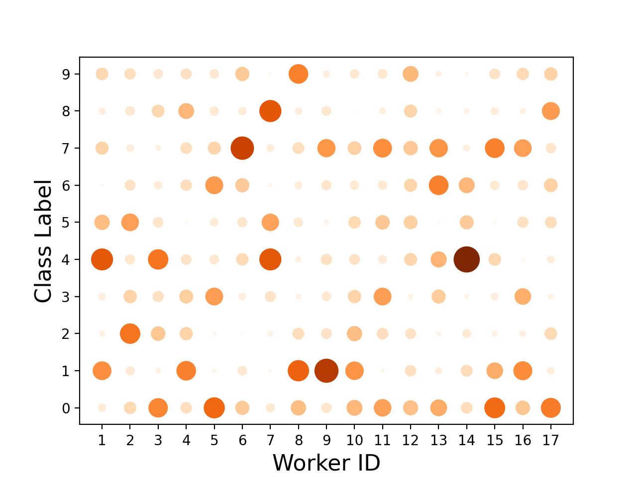
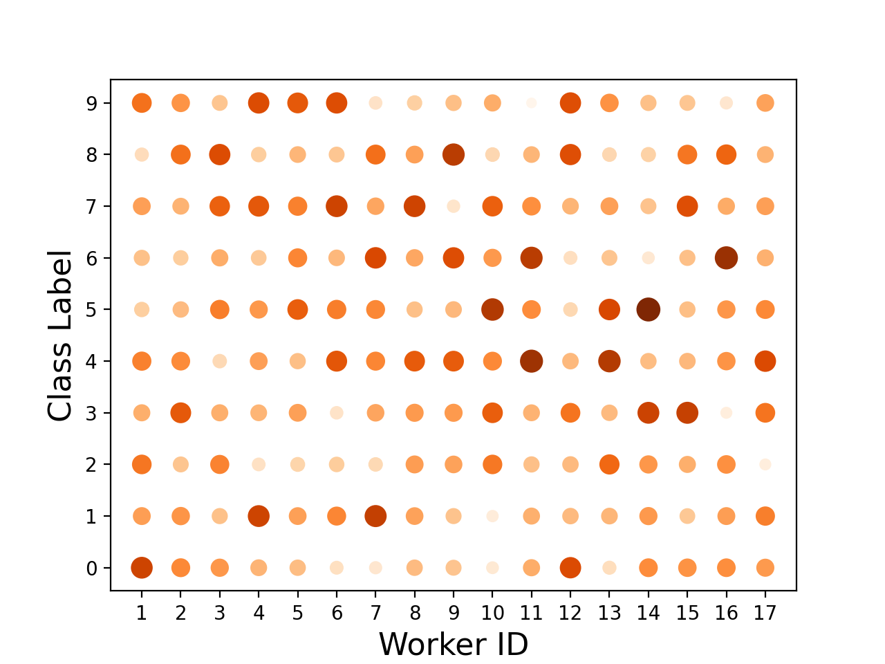
Figure 3: Distribution of data samples across workers and class labels on MNIST/CIFAR-10 when sampling from a Dirichlet distribution of parameter $\alpha$. Left: $\alpha=0.1$, Middle: $\alpha=1$, Right: $\alpha=10$.

15 Full Experimental Results

Section 15.1 presents our results on the MNIST dataset. Section 15.2 contains our results on Fashion-MNIST. Section 15.3 shows the performance of our algorithm on CIFAR-10.

15.1 Comprehensive Results on MNIST

In this section, we present the entirety of our results on the MNIST dataset.

15.1.1 Results on D-SHB

We consider three Byzantine regimes: $f=4$, $f=6$, and $f=8$ (largest possible) out of $n=17$ workers in total. We also consider three heterogeneity regimes: $\alpha=0.1$ (extreme), $\alpha=1$ (moderate), and $\alpha=10$ (low). We compare the performance of NNM and Bucketing when executed with four aggregation rules namely Krum [7], GM [43], CWMed [48], and CWTM [48]. The plots are presented below and complement our (partial) results in Table 2 in Section 6.2 of the main paper. We note that in the two strongest Byzantine settings, i.e., when $f>4$, Bucketing can only be applied with bucket size $s=1$ [26]. This means that when $f=6,8$, executing Bucketing boils down to running the vanilla aggregation rules.

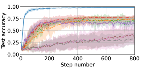
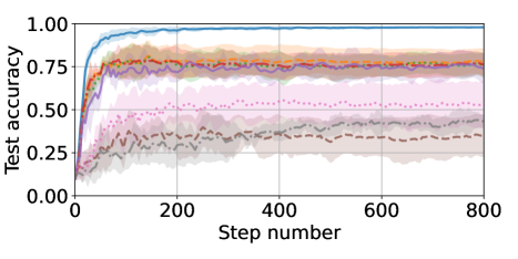
Figure 4: Experiments on MNIST using robust D-SHB with $f=4$ among $n=17$ workers, with $\beta=0.9$ and $\alpha=0.1$. The Byzantine workers execute FOE (row 1, left), ALIE (row 1, right), Mimic (row 2, left), SF (row 2, right), and LF (row 3).

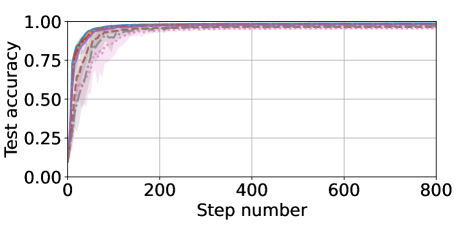
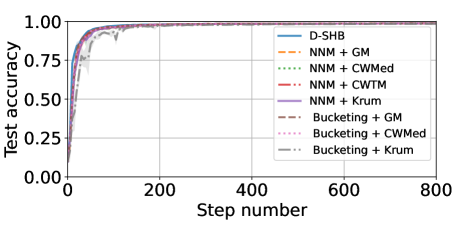
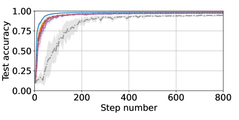
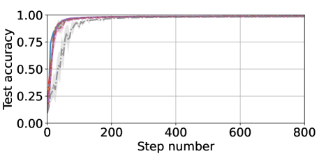
Figure 5: Experiments on MNIST using robust D-SHB with $f=4$ among $n=17$ workers, with $\beta=0.9$ and $\alpha=1$. The Byzantine workers execute FOE (row 1, left), ALIE (row 1, right), Mimic (row 2, left), SF (row 2, right), and LF (row 3).

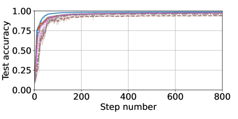
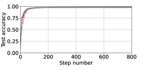
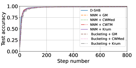
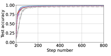
Figure 6: Experiments on MNIST using robust D-SHB with $f=4$ among $n=17$ workers, with $\beta=0.9$ and $\alpha=10$. The Byzantine workers execute FOE (row 1, left), ALIE (row 1, right), Mimic (row 2, left), SF (row 2, right), and LF (row 3).

Figure 7: Experiments on MNIST using robust D-SHB with $f=6$ among $n=17$ workers, with $\beta=0.9$ and $\alpha=1$. The Byzantine workers execute FOE (row 1, left), ALIE (row 1, right), Mimic (row 2, left), SF (row 2, right), and LF (row 3).

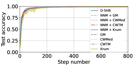
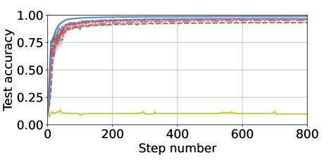
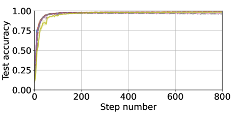
Figure 8: Experiments on MNIST using robust D-SHB with $f=6$ among $n=17$ workers, with $\beta=0.9$ and $\alpha=10$. The Byzantine workers execute FOE (row 1, left), ALIE (row 1, right), Mimic (row 2, left), SF (row 2, right), and LF (row 3).

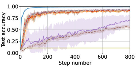
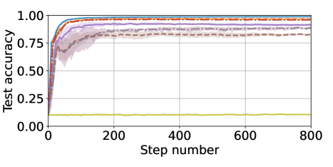
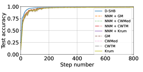
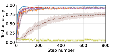
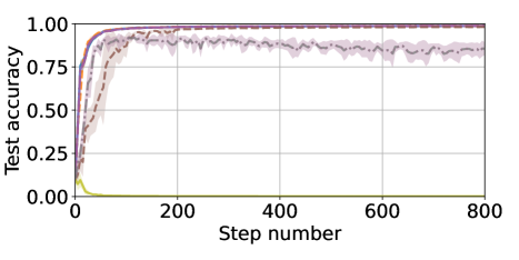
Figure 9: Experiments on MNIST using robust D-SHB with $f=8$ among $n=17$ workers, with $\beta=0.9$ and $\alpha=10$. The Byzantine workers execute FOE (row 1, left), ALIE (row 1, right), Mimic (row 2, left), SF (row 2, right), and LF (row 3).

15.1.2 Results on D-GD

We also test our algorithm with robust D-GD on MNIST in one Byzantine regime: $f=4$ Byzantine workers among a total of $n=17$ workers. We also consider three heterogeneity settings: $\alpha=0.1$, $\alpha=1$, and $\alpha=10$. The results are shown below, and convey the same observations made in Appendix 15.1.

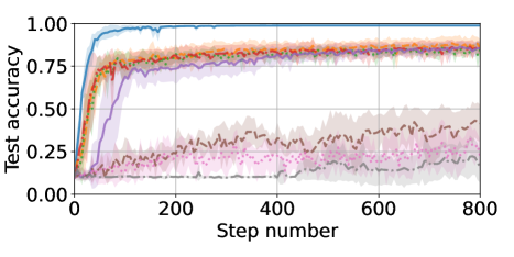
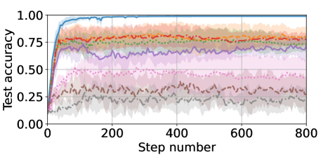
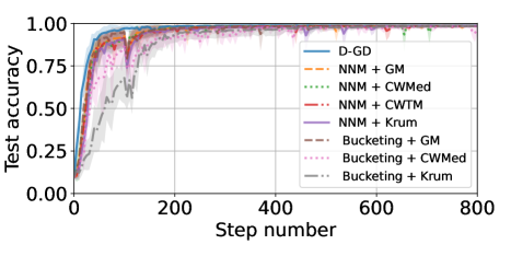
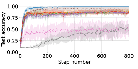
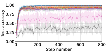
Figure 10: Experiments on MNIST using robust D-GD with $f=4$ among $n=17$ workers, with $\alpha=0.1$. The Byzantine workers execute the FOE (row 1, left), ALIE (row 1, right), Mimic (row 2, left), SF (row 2, right), and LF (row 3) attacks.

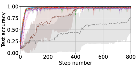
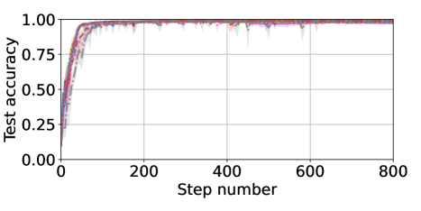
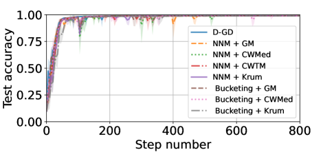
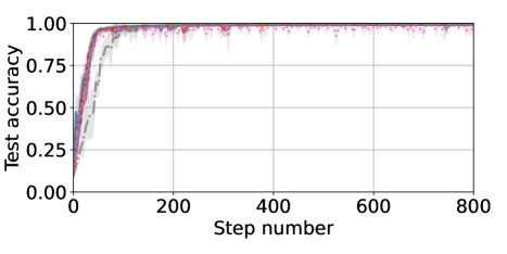
Figure 11: Experiments on MNIST using robust D-GD with $f=4$ among $n=17$ workers, with $\alpha=1$. The Byzantine workers execute the FOE (row 1, left), ALIE (row 1, right), Mimic (row 2, left), SF (row 2, right), and LF (row 3) attacks.

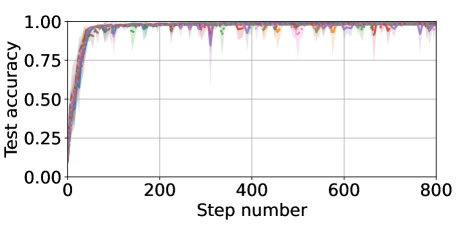
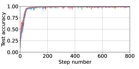
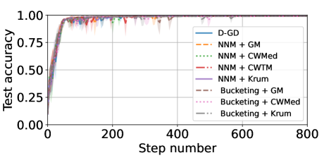
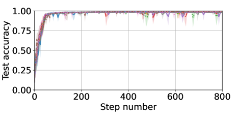
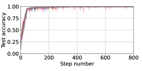
Figure 12: Experiments on MNIST using robust D-GD with $f=4$ among $n=17$ workers, with $\alpha=10$. The Byzantine workers execute the FOE (row 1, left), ALIE (row 1, right), Mimic (row 2, left), SF (row 2, right), and LF (row 3) attacks.

15.1.3 Results on Other Aggregation Rules: MDA, MultiKrum, and MeaMed

We also execute NNM with three additional aggregation rules namely MDA [40, 13], MeaMed [46], and Multi-Krum [7]. The experimental setup is the following. We consider three Byzantine regimes: $f=4$, $f=6$, and $f=8$ (largest possible) out of $n=17$ workers in total. We also consider three heterogeneity regimes: $\alpha=0.1$ (extreme), $\alpha=1$ (moderate), and $\alpha=10$ (low). We compare the performance of NNM and Bucketing when executed with MDA, MultiKrum, and MeaMed. The results (shown below) are very similar to the ones presented in Appendix 15.1, and convey exactly the same observations made in Section 6. Indeed, NNM combined with these methods provides consistently good performance on MNIST in three regimes of data heterogeneity and under five state-of-the-art Byzantine attacks. Given that no guarantees have yet been derived for these aggregation techniques, an interesting future direction would be to prove that MDA, MultiKrum, and MeaMed are $(f,\kappa)$-robust with $\kappa\in\mathcal{O}(1)$, confirming the modularity of our solution as a reliable framework for heterogeneous Byzantine learning.

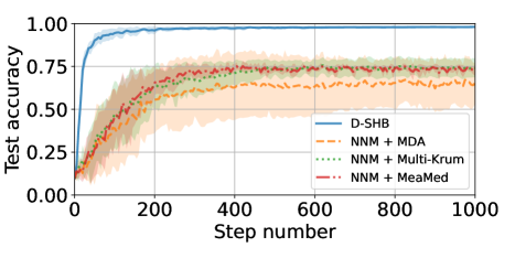
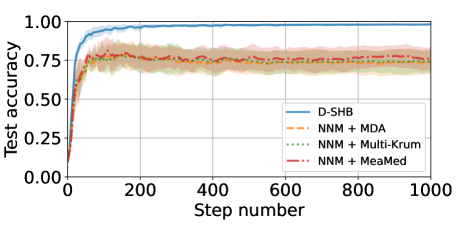
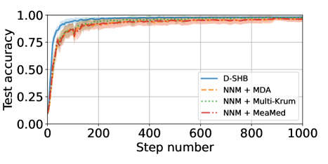
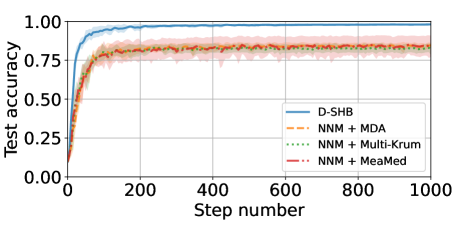
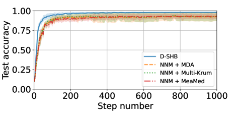
Figure 13: Experiments on MNIST using robust D-SHB with $f=4$ Byzantine among $n=17$ workers, with $\beta=0.9$ and $\alpha=0.1$. The Byzantine workers execute the FOE (row 1, left), ALIE (row 1, right), Mimic (row 2, left), SF (row 2, right), and LF (row 3) attacks.

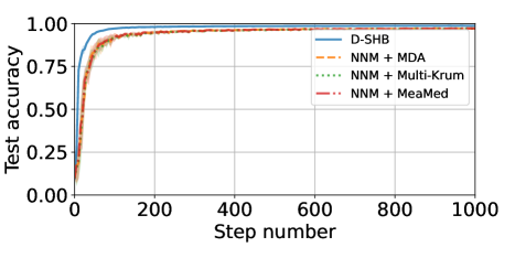
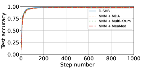
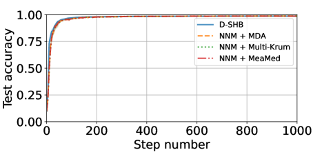
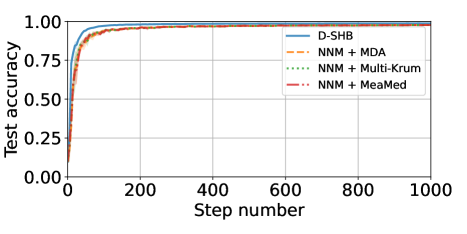
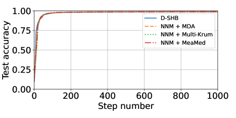
Figure 14: Experiments on MNIST using robust D-SHB with $f=4$ Byzantine among $n=17$ workers, with $\beta=0.9$ and $\alpha=1$. The Byzantine workers execute the FOE (row 1, left), ALIE (row 1, right), Mimic (row 2, left), SF (row 2, right), and LF (row 3) attacks.

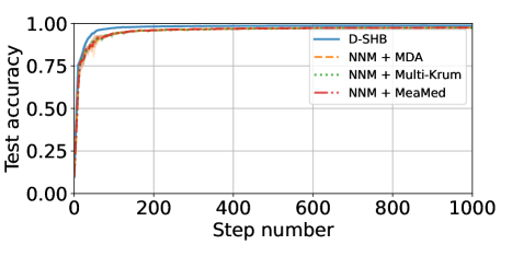
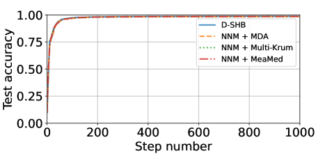
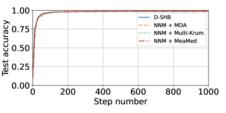
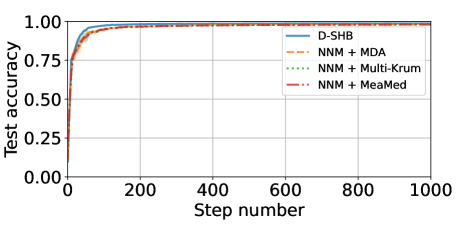
Figure 15: Experiments on MNIST using robust D-SHB with $f=4$ Byzantine among $n=17$ workers, with $\beta=0.9$ and $\alpha=10$. The Byzantine workers execute the FOE (row 1, left), ALIE (row 1, right), Mimic (row 2, left), SF (row 2, right), and LF (row 3) attacks.

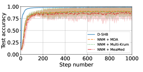
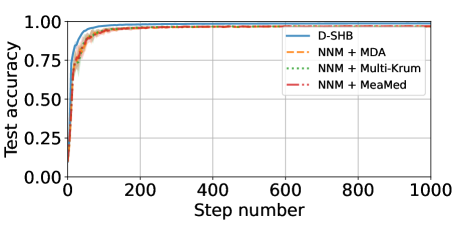
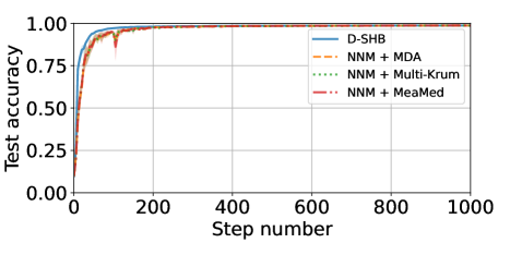
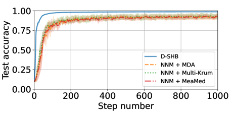
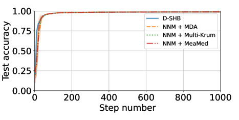
Figure 16: Experiments on MNIST using robust D-SHB with $f=6$ Byzantine among $n=17$ workers, with $\beta=0.9$ and $\alpha=1$. The Byzantine workers execute the FOE (row 1, left), ALIE (row 1, right), Mimic (row 2, left), SF (row 2, right), and LF (row 3) attacks.

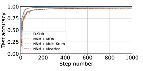
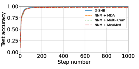
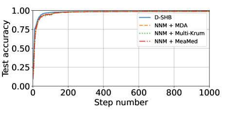
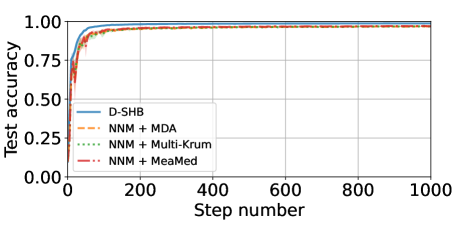
Figure 17: Experiments on MNIST using robust D-SHB with $f=6$ Byzantine among $n=17$ workers, with $\beta=0.9$ and $\alpha=10$. The Byzantine workers execute the FOE (row 1, left), ALIE (row 1, right), Mimic (row 2, left), SF (row 2, right), and LF (row 3) attacks.

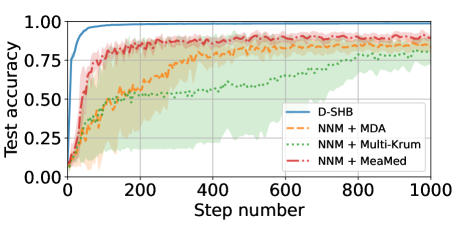
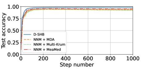
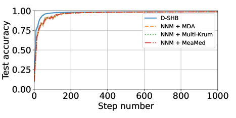
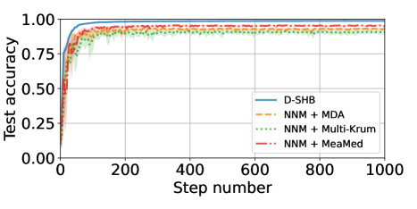
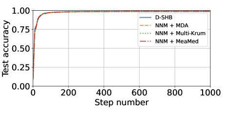
Figure 18: Experiments on MNIST using robust D-SHB with $f=8$ Byzantine among $n=17$ workers, with $\beta=0.9$ and $\alpha=10$. The Byzantine workers execute the FOE (row 1, left), ALIE (row 1, right), Mimic (row 2, left), SF (row 2, right), and LF (row 3) attacks.

15.2 Comprehensive Results on Fashion-MNIST

In this section, we showcase our results on the Fashion-MNIST dataset. We consider two Byzantine regimes: $f=4$ and $f=6$ out of $n=17$ workers in total. We also consider three heterogeneity regimes: $\alpha=0.1$ (extreme), $\alpha=1$ (moderate), and $\alpha=10$ (low). We plots compare the performance of NNM and Bucketing when executed with four aggregation rules namely Krum, GM, CWMed, and CWTM. The plots are presented below. We note that in the strongest Byzantine setting, i.e., when $f>4$, Bucketing can only be applied with bucket size $s=1$ [26]. This means that when $f=6$, executing Bucketing boils down to running the vanilla aggregation rules.

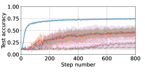
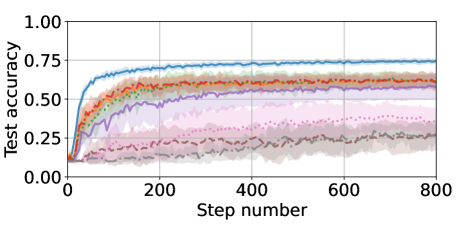
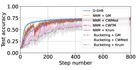
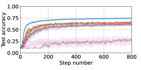
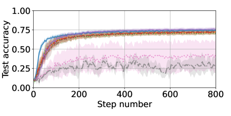
Figure 19: Experiments on Fashion-MNIST using robust D-SHB with $f=4$ Byzantine among $n=17$ workers, with $\beta=0.9$ and $\alpha=0.1$. The Byzantine workers execute the FOE (row 1, left), ALIE (row 1, right), Mimic (row 2, left), SF (row 2, right), and LF (row 3) attacks.

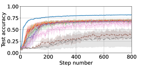
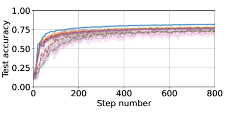
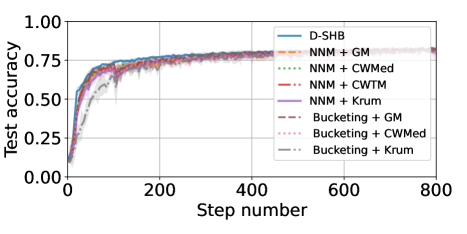
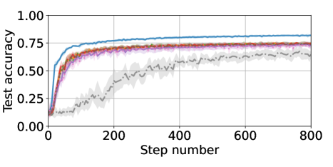
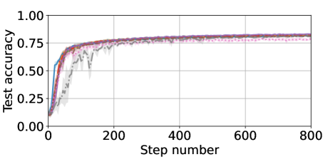
Figure 20: Experiments on Fashion-MNIST using robust D-SHB with $f=4$ Byzantine among $n=17$ workers, with $\beta=0.9$ and $\alpha=1$. The Byzantine workers execute the FOE (row 1, left), ALIE (row 1, right), Mimic (row 2, left), SF (row 2, right), and LF (row 3) attacks.

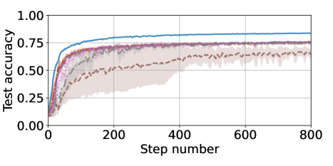
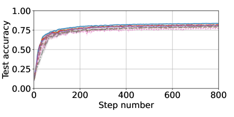
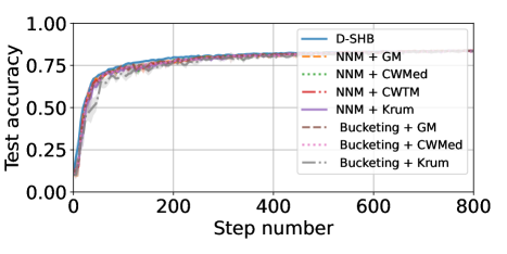
Figure 21: Experiments on Fashion-MNIST using robust D-SHB with $f=4$ Byzantine among $n=17$ workers, with $\beta=0.9$ and $\alpha=10$. The Byzantine workers execute the FOE (row 1, left), ALIE (row 1, right), Mimic (row 2, left), SF (row 2, right), and LF (row 3) attacks.

Figure 22: Experiments on Fashion-MNIST using robust D-SHB with $f=6$ Byzantine among $n=17$ workers, with $\beta=0.9$ and $\alpha=1$. The Byzantine workers execute the FOE (row 1, left), ALIE (row 1, right), Mimic (row 2, left), SF (row 2, right), and LF (row 3) attacks.

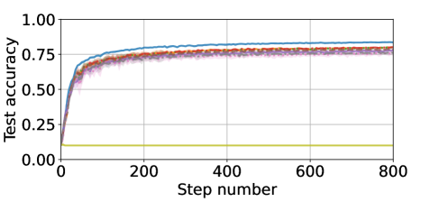
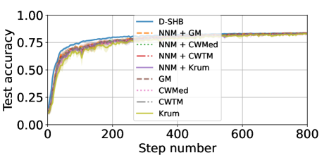
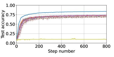
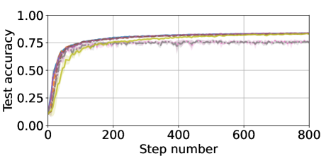
Figure 23: Experiments on Fashion-MNIST using robust D-SHB with $f=6$ Byzantine among $n=17$ workers, with $\beta=0.9$ and $\alpha=10$. The Byzantine workers execute the FOE (row 1, left), ALIE (row 1, right), Mimic (row 2, left), SF (row 2, right), and LF (row 3) attacks.

15.3 Comprehensive Results on CIFAR-10

In this section, we present the entirety of our results on CIFAR-10. We consider three Byzantine regimes: $f=2$, $f=3$, and $f=4$ out of $n=17$ workers in total. We also consider two heterogeneity regimes: $\alpha=1$ (moderate), and $\alpha=10$ (low). We compare the performance of NNM and Bucketing when executed with four aggregation rules namely Krum, GM, CWMed, and CWTM. The plots are presented below and complement our (partial) results in Figure 1 in Section 6.3 of the main paper.

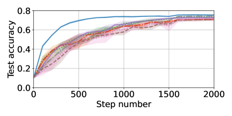
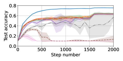
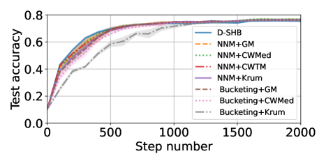
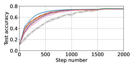
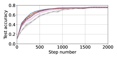
Figure 24: Experiments on CIFAR-10 using robust D-SHB with $f=2$ Byzantine among $n=17$ workers, with $\beta=0.9$ and $\alpha=1$. The Byzantine workers execute the FOE (row 1, left), ALIE (row 1, right), Mimic (row 2, left), SF (row 2, right), and LF (row 3) attacks.

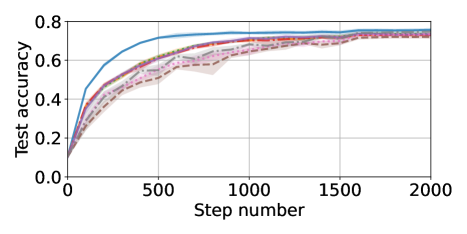
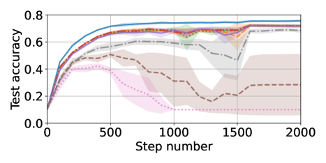
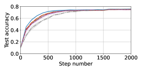
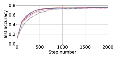
Figure 25: Experiments on CIFAR-10 using robust D-SHB with $f=2$ Byzantine among $n=17$ workers, with $\beta=0.9$ and $\alpha=10$. The Byzantine workers execute the FOE (row 1, left), ALIE (row 1, right), Mimic (row 2, left), SF (row 2, right), and LF (row 3) attacks.

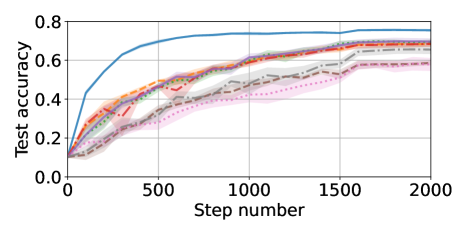
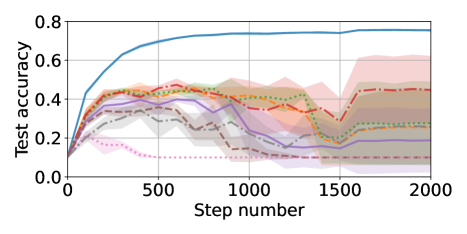
Figure 26: Experiments on CIFAR-10 using robust D-SHB with $f=3$ Byzantine among $n=17$ workers, with $\beta=0.9$ and $\alpha=1$. The Byzantine workers execute the FOE (row 1, left), ALIE (row 1, right), Mimic (row 2, left), SF (row 2, right), and LF (row 3) attacks.

Figure 27: Experiments on CIFAR-10 using robust D-SHB with $f=3$ Byzantine among $n=17$ workers, with $\beta=0.9$ and $\alpha=10$. The Byzantine workers execute the FOE (row 1, left), ALIE (row 1, right), Mimic (row 2, left), SF (row 2, right), and LF (row 3) attacks.

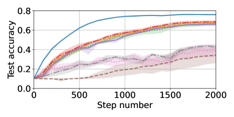
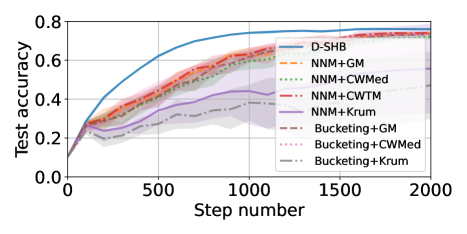
Figure 28: Experiments on CIFAR-10 using robust D-SHB with $f=4$ Byzantine among $n=17$ workers, with $\beta=0.99$ and $\alpha=10$. The Byzantine workers execute the FOE (row 1, left), ALIE (row 1, right), Mimic (row 2, left), SF (row 2, right), and LF (row 3) attacks.

References

• [1] Martín Abadi, Ashish Agarwal, Paul Barham, Eugene Brevdo, Zhifeng Chen, Craig Citro, Greg Corrado, Andy Davis, Jeffrey Dean, Matthieu Devin, Sanjay Ghemawat, Ian Goodfellow, Andrew Harp, Geoffrey Irving, Michael Isard, Yangqing Jia, Rafal Jozefowicz, Lukasz Kaiser, Manjunath Kudlur, Josh Levenberg, Dan Mané, Rajat Monga, Sherry Moore, Derek Murray, Chris Olah, Mike Schuster, Jonathon Shlens, Benoit Steiner, Ilya Sutskever, Kunal Talwar, Paul Tucker, Vincent Vanhoucke, Vijay Vasudevan, Fernanda Viégas, Oriol Vinyals, Pete Warden, Martin Wattenberg, Martin Wicke, Yuan Yu, and Xiaoqiang Zheng. Tensorflow: Large-scale machine learning on heterogeneous distributed systems, 2015.
• [2] Anish Acharya, Abolfazl Hashemi, Prateek Jain, Sujay Sanghavi, Inderjit S. Dhillon, and Ufuk Topcu. Robust training in high dimensions via block coordinate geometric median descent. In Gustau Camps-Valls, Francisco J. R. Ruiz, and Isabel Valera, editors, Proceedings of The 25th International Conference on Artificial Intelligence and Statistics, volume 151 of Proceedings of Machine Learning Research, pages 11145–11168. PMLR, 28–30 Mar 2022.
• [3] Zeyuan Allen-Zhu, Faeze Ebrahimianghazani, Jerry Li, and Dan Alistarh. Byzantine-resilient non-convex stochastic gradient descent. In International Conference on Learning Representations, 2020.
• [4] Noga Alon, Yossi Matias, and Mario Szegedy. The space complexity of approximating the frequency moments. In Proceedings of the twenty-eighth annual ACM symposium on Theory of computing, pages 20–29, 1996.
• [5] Moran Baruch, Gilad Baruch, and Yoav Goldberg. A little is enough: Circumventing defenses for distributed learning. In Advances in Neural Information Processing Systems 32: Annual Conference on Neural Information Processing Systems 2019, 8-14 December 2019, Long Beach, CA, USA, 2019.
• [6] Dimitri Bertsekas and John Tsitsiklis. Parallel and distributed computation: numerical methods. Athena Scientific, 2015.
• [7] Peva Blanchard, El Mahdi El Mhamdi, Rachid Guerraoui, and Julien Stainer. Machine learning with adversaries: Byzantine tolerant gradient descent. In I. Guyon, U. V. Luxburg, S. Bengio, H. Wallach, R. Fergus, S. Vishwanathan, and R. Garnett, editors, Advances in Neural Information Processing Systems 30, pages 119–129. Curran Associates, Inc., 2017.
• [8] Léon Bottou, Frank E Curtis, and Jorge Nocedal. Optimization methods for large-scale machine learning. Siam Review, 60(2):223–311, 2018.
• [9] Stephen Boyd and Lieven Vandenberghe. Convex optimization. Cambridge university press, 2004.
• [10] Moses Charikar, Jacob Steinhardt, and Gregory Valiant. Learning from untrusted data. In Proceedings of the 49th Annual ACM SIGACT Symposium on Theory of Computing, pages 47–60, 2017.
• [11] Yudong Chen, Lili Su, and Jiaming Xu. Distributed statistical machine learning in adversarial settings: Byzantine gradient descent. Proc. ACM Meas. Anal. Comput. Syst., 1(2), dec 2017.
• [12] Simon S Du, Chi Jin, Jason D Lee, Michael I Jordan, Aarti Singh, and Barnabas Poczos. Gradient descent can take exponential time to escape saddle points. Advances in neural information processing systems, 30, 2017.
• [13] El Mahdi El Mhamdi, Sadegh Farhadkhani, Rachid Guerraoui, Arsany Guirguis, Lê Nguyên Hoang, and Sébastien Rouault. Collaborative learning in the jungle (decentralized, byzantine, heterogeneous, asynchronous and nonconvex learning). In Thirty-Fifth Conference on Neural Information Processing Systems, 2021.
• [14] El Mahdi El Mhamdi, Rachid Guerraoui, and Sébastien Rouault. The hidden vulnerability of distributed learning in Byzantium. In Jennifer Dy and Andreas Krause, editors, Proceedings of the 35th International Conference on Machine Learning, volume 80 of Proceedings of Machine Learning Research, pages 3521–3530. PMLR, 10–15 Jul 2018.
• [15] El Mahdi El Mhamdi, Rachid Guerraoui, and Sébastien Louis Alexandre Rouault. Distributed momentum for byzantine-resilient stochastic gradient descent. In 9th International Conference on Learning Representations (ICLR), number CONF, 2021.
• [16] Sadegh Farhadkhani, Rachid Guerraoui, Nirupam Gupta, Lê Nguyên Hoang, Rafael Pinot, and John Stephan. Making byzantine decentralized learning efficient. arXiv preprint arXiv:2209.10931, 2022.
• [17] Sadegh Farhadkhani, Rachid Guerraoui, Nirupam Gupta, Rafael Pinot, and John Stephan. Byzantine machine learning made easy by resilient averaging of momentums. In Kamalika Chaudhuri, Stefanie Jegelka, Le Song, Csaba Szepesvari, Gang Niu, and Sivan Sabato, editors, Proceedings of the 39th International Conference on Machine Learning, volume 162 of Proceedings of Machine Learning Research, pages 6246–6283. PMLR, 17–23 Jul 2022.
• [18] Sébastien Gadat, Fabien Panloup, and Sofiane Saadane. Stochastic heavy ball. Electronic Journal of Statistics, 12(1):461–529, 2018.
• [19] Saeed Ghadimi and Guanghui Lan. Accelerated gradient methods for nonconvex nonlinear and stochastic programming. Mathematical Programming, 156(1):59–99, 2016.
• [20] Nirupam Gupta and Nitin H Vaidya. Fault-tolerance in distributed optimization: The case of redundancy. In Proceedings of the 39th Symposium on Principles of Distributed Computing, pages 365–374, 2020.
• [21] Kiana Hajebi, Yasin Abbasi-Yadkori, Hossein Shahbazi, and Hong Zhang. Fast approximate nearest-neighbor search with k-nearest neighbor graph. In Twenty-Second International Joint Conference on Artificial Intelligence, 2011.
• [22] Tzu-Ming Harry Hsu, Hang Qi, and Matthew Brown. Measuring the effects of non-identical data distribution for federated visual classification, 2019.
• [23] Mark R Jerrum, Leslie G Valiant, and Vijay V Vazirani. Random generation of combinatorial structures from a uniform distribution. Theoretical computer science, 43:169–188, 1986.
• [24] Peter Kairouz, H. Brendan McMahan, Brendan Avent, Aurélien Bellet, Mehdi Bennis, Arjun Nitin Bhagoji, Kallista Bonawitz, Zachary Charles, Graham Cormode, Rachel Cummings, Rafael G. L. D’Oliveira, Hubert Eichner, Salim El Rouayheb, David Evans, Josh Gardner, Zachary Garrett, Adrià Gascón, Badih Ghazi, Phillip B. Gibbons, Marco Gruteser, Zaid Harchaoui, Chaoyang He, Lie He, Zhouyuan Huo, Ben Hutchinson, Justin Hsu, Martin Jaggi, Tara Javidi, Gauri Joshi, Mikhail Khodak, Jakub Konecný, Aleksandra Korolova, Farinaz Koushanfar, Sanmi Koyejo, Tancrède Lepoint, Yang Liu, Prateek Mittal, Mehryar Mohri, Richard Nock, Ayfer Özgür, Rasmus Pagh, Hang Qi, Daniel Ramage, Ramesh Raskar, Mariana Raykova, Dawn Song, Weikang Song, Sebastian U. Stich, Ziteng Sun, Ananda Theertha Suresh, Florian Tramèr, Praneeth Vepakomma, Jianyu Wang, Li Xiong, Zheng Xu, Qiang Yang, Felix X. Yu, Han Yu, and Sen Zhao. Advances and open problems in federated learning. Foundations and Trends® in Machine Learning, 14(1–2):1–210, 2021.
• [25] Sai Praneeth Karimireddy, Lie He, and Martin Jaggi. Learning from history for byzantine robust optimization. International Conference On Machine Learning, Vol 139, 139, 2021.
• [26] Sai Praneeth Karimireddy, Lie He, and Martin Jaggi. Byzantine-robust learning on heterogeneous datasets via bucketing. In International Conference on Learning Representations, 2022.
• [27] Sai Praneeth Karimireddy, Satyen Kale, Mehryar Mohri, Sashank Reddi, Sebastian Stich, and Ananda Theertha Suresh. Scaffold: Stochastic controlled averaging for federated learning. In International Conference on Machine Learning, pages 5132–5143. PMLR, 2020.
• [28] Jakub Konečnỳ, H Brendan McMahan, Felix X Yu, Peter Richtárik, Ananda Theertha Suresh, and Dave Bacon. Federated learning: Strategies for improving communication efficiency. arXiv preprint arXiv:1610.05492, 2016.
• [29] Alex Krizhevsky, Vinod Nair, and Geoffrey Hinton. The cifar-10 dataset. online: http://www. cs. toronto. edu/kriz/cifar. html, 55(5), 2014.
• [30] Leslie Lamport, Robert Shostak, and Marshall Pease. The byzantine generals problem. ACM Trans. Program. Lang. Syst., 4(3):382–401, jul 1982.
• [31] Yann LeCun and Corinna Cortes. MNIST handwritten digit database. 2010.
• [32] Liping Li, Wei Xu, Tianyi Chen, Georgios B. Giannakis, and Qing Ling. Rsa: Byzantine-robust stochastic aggregation methods for distributed learning from heterogeneous datasets. In Proceedings of the Thirty-Third AAAI Conference on Artificial Intelligence and Thirty-First Innovative Applications of Artificial Intelligence Conference and Ninth AAAI Symposium on Educational Advances in Artificial Intelligence, AAAI’19/IAAI’19/EAAI’19. AAAI Press, 2019.
• [33] Jun Liu and Ye Yuan. On almost sure convergence rates of stochastic gradient methods. In Po-Ling Loh and Maxim Raginsky, editors, Proceedings of Thirty Fifth Conference on Learning Theory, volume 178 of Proceedings of Machine Learning Research, pages 2963–2983. PMLR, 02–05 Jul 2022.
• [34] Shuo Liu, Nirupam Gupta, and Nitin H. Vaidya. Approximate byzantine fault-tolerance in distributed optimization. In Proceedings of the 2021 ACM Symposium on Principles of Distributed Computing, PODC’21, page 379–389, New York, NY, USA, 2021. Association for Computing Machinery.
• [35] Marius Muja and David G Lowe. Scalable nearest neighbor algorithms for high dimensional data. IEEE transactions on pattern analysis and machine intelligence, 36(11):2227–2240, 2014.
• [36] A.S. Nemirovsky, D.B. din, and D.B. Yudin. Problem Complexity and Method Efficiency in Optimization. A Wiley-Interscience publication. Wiley, 1983.
• [37] Yurii Nesterov et al. Lectures on convex optimization, volume 137. Springer, 2018.
• [38] Krishna Pillutla, Sham M. Kakade, and Zaid Harchaoui. Robust aggregation for federated learning. IEEE Transactions on Signal Processing, 70:1142–1154, 2022.
• [39] Boris T Polyak. Some methods of speeding up the convergence of iteration methods. Ussr computational mathematics and mathematical physics, 4(5):1–17, 1964.
• [40] Peter J Rousseeuw. Multivariate estimation with high breakdown point. Mathematical statistics and applications, 8(37):283–297, 1985.
• [41] Othmane Sebbouh, Robert M Gower, and Aaron Defazio. Almost sure convergence rates for stochastic gradient descent and stochastic heavy ball. In Conference on Learning Theory, pages 3935–3971. PMLR, 2021.
• [42] Virat Shejwalkar and Amir Houmansadr. Manipulating the byzantine: Optimizing model poisoning attacks and defenses for federated learning. In NDSS, 2021.
• [43] Christopher G Small. A survey of multidimensional medians. International Statistical Review/Revue Internationale de Statistique, pages 263–277, 1990.
• [44] Jiyuan Tu, Weidong Liu, Xiaojun Mao, and Xi Chen. Variance reduced median-of-means estimator for byzantine-robust distributed inference. J. Mach. Learn. Res., 22:84–1, 2021.
• [45] Han Xiao, Kashif Rasul, and Roland Vollgraf. Fashion-mnist: a novel image dataset for benchmarking machine learning algorithms. arXiv preprint arXiv:1708.07747, 2017.
• [46] Cong Xie, Oluwasanmi Koyejo, and Indranil Gupta. Generalized byzantine-tolerant sgd, 2018.
• [47] Cong Xie, Oluwasanmi Koyejo, and Indranil Gupta. Fall of empires: Breaking byzantine-tolerant SGD by inner product manipulation. In Proceedings of the Thirty-Fifth Conference on Uncertainty in Artificial Intelligence, UAI 2019, Tel Aviv, Israel, July 22-25, 2019, page 83, 2019.
• [48] Dong Yin, Yudong Chen, Ramchandran Kannan, and Peter Bartlett. Byzantine-robust distributed learning: Towards optimal statistical rates. In Jennifer Dy and Andreas Krause, editors, Proceedings of the 35th International Conference on Machine Learning, volume 80 of Proceedings of Machine Learning Research, pages 5650–5659. PMLR, 10–15 Jul 2018.