Hyperfine splittings of heavy quarkonium hybrids

Abstract

In the framework of the Born-Oppenheimer Effective Field Theory, the hyperfine structure of heavy quarkonium hybrids at leading order in the $1/m_{Q}$ expansion is determined by two potentials. We estimate those potentials by interpolating between the known short distance behavior and the long distance behavior calculated in the QCD Effective String Theory. The long distance behavior depends, at leading order, on two parameters which can be obtained from the long distance behavior of the heavy quarkonium potentials (up to sign ambiguities). The short distance behavior depends, at leading order, on two extra paramentes, which are obtained from a lattice calculation of the lower lying charmonium hybrid multiplets. This allows us to predict the hyperfine splitting both of bottomonium hybrids and of higher multiplets of charmonium hybrids. We carry out a careful error analysis and compare with other approaches.

I Introduction

Exotic hadrons (those beyond mesons and baryons) have been a matter of research since the early days of QCD Jaffe:1975fd . Among them, the so called hybrids are the closests to standard hadrons, as the only difference resides in their non-trivial gluon content. Hence their flavor structure is the same as in standard hadrons, but their $J^{PC}$ quantum numbers may differ since, in general, the non-trivial gluon content contributes to them. Nevertheless, the experimental confirmation of hybrids is an arduous task. On the one hand, hadrons with exotic quantum numbers, which could be associated to hybrid states, are difficult to produce with current beams. On the other hand, for light hadrons, hybrids with standard quantum numbers may mix with standard hadrons in an arbitrary way. However, when heavy quarks are involved the mixing is suppressed by inverse powers of the heavy quark mass, and hence the identification of hybrids with standard quantum numbers should become simpler, provided we have reliable theoretical predictions for the hybrid spectrum.

An economical approach to calculating the hybrid spectrum is the so-called Born-Oppenheimer effective field theory (BOEFT) Braaten:2014qka ; Berwein:2015vca ; Oncala:2017hop ; Soto:2017one ; Brambilla:2018pyn ; Soto:2020xpm . It exploits the fact that heavy quarks move slowly in heavy hadrons. The effect of the nontrivial gluon (or/and light quark) content is encoded in a series of potentials organized in an $1/m_{Q}$ expansion, $m_{Q}$ being the heavy quark mass. The leading potential ($\mathcal{O}(1/m_{Q}^{0})$) is heavy quark spin and heavy quark mass independent. It has been used to calculate the spin average spectrum Juge:1999ie ; Braaten:2014qka ; Berwein:2015vca ; Oncala:2017hop , decays to heavy quarkonium Braaten:2014ita ; Oncala:2017hop ; TarrusCastella:2021pld ; Brambilla:2022hhi , and transitions between heavy quarkonium states Pineda:2019mhw . The mixing of heavy quarkonium hybrids with heavy quarkonium starts at order $1/m_{Q}$ Oncala:2017hop . Spin effects also start at order $1/m_{Q}$ Oncala:2017hop ; Soto:2017one , and hence, they are more important than in heavy quarkonium, in which they start at order $1/m_{Q}^{2}$. In that respect, it is important to have spin effects under good control in order to properly identify possible experimental candidates (see Brambilla:2019esw ; Chen:2022asf for recent reviews).

We calculate here the hyperfine splittings (HFS) for the lower lying charmonium and bottomonium hybrids at leading-order (LO) ($\mathcal{O}(1/m_{Q})$) in the BOEFT. At this order, the HFS depend on two unknown potentials Soto:2017one ; Brambilla:2018pyn . At short distances the form of these potentials is constrained by the multipole expansion and has been given in ref. Brambilla:2018pyn ; Brambilla:2019jfi , where one can also find the form of the relevant next-to-leading order (NLO) potentials ($\mathcal{O}(1/m_{Q}^{2})$). The HFS was calculated in that reference using the short distance form of the potentials only. At long distances, the form of the potentials can be estimated using the QCD effective string theory (EST) Luscher:2002qv ; Luscher:2004ib . This has been carried out for heavy quarkonium Perez-Nadal:2008wtr ; Brambilla:2014eaa and for the hybrid-quarkonium mixing terms Oncala:2017hop . We provide the results here for the spin-dependent terms of the lower lying static hybrid states ($\Sigma_{u}$ and $\Pi_{u}$), which turn out to be parameter free (up to signs). We emphasize that the typical distance between heavy quarks in heavy quarkonium hybrids states is of $\mathcal{O}(1/\Lambda_{\rm QCD})$, and hence an interpolation between the short and long distance forms of the spin-dependent potentials should provide more reliable estimates than sticking to the short distance form only. We propose a simple interpolation and calculate the HFS with it. We use the charmonium spectrum of ref. Cheung:2016bym to fix the unknown parameters in the short distance form of the potential, and to estimate the interpolation dependence. Then we can predict the HFS of higher multiplets and the HFS of bottomonium hybrids.

We distribute the paper as follows. In Section II, we work out the structure of the spin-dependent terms in a convenient basis. We specify the form of the spin-dependent potentials at short distances in III.1, at long distances in III.2, and the interpolation we use in III.3. In Section IV, we fix our free parameters using hybrid charmonium lattice data for the lower multiplets and obtain the HFS of higher multiplets. In Section V, we obtain the HFS of bottomonium hybrids. Section VI is devoted to the comparison with other approaches and we close with a discussion and our conclusions in Section VII.

II The hyperfine splittings

General expressions for the BOEFT at NLO have been recently obtained in ref. Soto:2020xpm . The lower lying hybrid potentials correspond to the $\kappa^{p}=1^{+}$ quantum numbers of the light degrees of freedom (LDOF), where $\kappa$ is the total angular momentum and $p$ the parity. We focus on the heavy quark spin-dependent terms in the Hamiltonian $V_{\kappa^{p}}^{(1)}(\mathbf{r})/m_{Q}$,

$$V_{\kappa^{p}}^{(1)}(\mathbf{r}) = \sum_{\Lambda\Lambda^{\prime}}{\cal P}_{\kappa\Lambda}\left[V^{sa}_{\kappa^{p}\Lambda\Lambda^{\prime}}(r)\bm{S}_{Q\bar{Q}}\cdot\left({\cal P}_{10}\cdot\bm{S}_{\kappa}\right)\right.$$ (1)

$$+ \left.V^{sb}_{\kappa^{p}\Lambda\Lambda^{\prime}}(r)\bm{S}_{Q\bar{Q}}\cdot\left({\cal P}_{11}\cdot\bm{S}_{\kappa}\right)\right]{\cal P}_{\kappa\Lambda^{\prime}}\,,$$

where $\bm{S}_{Q\bar{Q}}$ and $\bm{S}_{\kappa}$ are the spin operators of the heavy quark-antiquark pair and the total angular momentum operator of the LDOF respectively. ${\cal P}_{\kappa\Lambda}$ are the projectors to the irreducible representations of the $D_{h\infty}$ group $\Lambda=0,1$. They read,

$${\cal P}_{10} = \mathbb{I}_{3}-\left(\hat{\bm{r}}\cdot\bm{S}_{1}\right)^{2}\,,$$

$${\cal P}_{11} = \left(\hat{\bm{r}}\cdot\bm{S}_{1}\right)^{2}$$ (2)

In our case, the above potentials act on fields $H^{nm}_{1}(\mathbf{r},t)$, $n,m=1,2,3$, where the first index corresponds to the total angular momentum of the LDOF and the second to the spin of the heavy quark-antiquark pair. In the Cartesian basis, $\left(\bm{S}_{1}^{i}\right)^{jk}=-i\epsilon^{ijk}$, we then have,

$${\cal P}_{10}^{n^{\prime}n} = \hat{r}^{n^{\prime}}\hat{r}^{n}\,,$$

$${\cal P}_{11}^{n^{\prime}n} = \delta^{n^{\prime}n}-\hat{r}^{n^{\prime}}\hat{r}^{n}$$ (3)

Analogously, the heavy quark-antiquark spin operators read $\left(\bm{S}_{Q\bar{Q}}^{i}\right)^{m^{\prime}m}=-i\epsilon_{im^{\prime}m}$ . We find that only two independent potentials survive.

$$\left[V_{\kappa^{p}}^{(1)}(\bm{r})\right]^{n^{\prime}m^{\prime};\,nm}=-V^{sa}_{1^{+}11}(r)\left(\delta^{n^{\prime}m}\delta^{nm^{\prime}}-\delta^{n^{\prime}m^{\prime}}\delta^{nm}\right)$$

$$+\left(V^{sa}_{1^{+}11}(r)+V^{sb}_{1^{+}10}(r)\right)\hat{r}^{i}\hat{r}^{j}\left(\delta^{jm}\delta^{n^{\prime}i}\delta^{nm^{\prime}}+\right.$$

$$\left.+\delta^{ni}\delta^{jm^{\prime}}\delta^{n^{\prime}m}-\delta^{jm^{\prime}}\delta^{n^{\prime}i}\delta^{nm}-\delta^{ni}\delta^{jm}\delta^{n^{\prime}m^{\prime}}\right)$$

$$=-2V_{hf}(r)\left(\delta^{n^{\prime}m}\delta^{nm^{\prime}}-\delta^{n^{\prime}m^{\prime}}\delta^{nm}\right)$$ (4)

$$-2V_{hf2}(r)\left(\hat{r}^{i}\hat{r}^{j}-\frac{\delta^{ij}}{3}\right)\left(\delta^{jm}\delta^{n^{\prime}i}\delta^{nm^{\prime}}+\right.$$

$$\left.+\delta^{ni}\delta^{jm^{\prime}}\delta^{n^{\prime}m}-\delta^{jm^{\prime}}\delta^{n^{\prime}i}\delta^{nm}-\delta^{ni}\delta^{jm}\delta^{n^{\prime}m^{\prime}}\right)\,,$$

where we have used that time reversal and Hermiticity imply $V^{sb}_{1^{+}01}(r)=V^{sb}_{1^{+}10}(r)\in\mathbb{R}$, and we have defined,

$$V_{hf}(r) = \frac{1}{6}V^{sa}_{1^{+}11}(r)-\frac{1}{3}V^{sb}_{1^{+}10}(r)$$

$$V_{hf2}(r) = -\frac{1}{2}\left(V^{sa}_{1^{+}11}(r)+V^{sb}_{1^{+}10}(r)\right)$$ (5)

The structure leading to $V_{hf}$ was first noticed in Oncala:2017hop and the one leading to $V_{hf2}$ was already considered in the short distance analysis of Refs. Brambilla:2018pyn ; TarrusCastella:2019lyq . We write the field $H^{nm}_{1}(\mathbf{r},t)$ in the $|SLJ\mathcal{J}\mathcal{M}>$ basis, where $S$ and $L$ are the spin and the orbital angular momentum of the $Q\bar{Q}$ pair respectively, $J$ the total angular momentum of the LDOF plus the orbital angular momentum of the $Q\bar{Q}$, and $\mathcal{J}$ and $\mathcal{M}$ the total angular momentum and its third component respectively Oncala:2017hop . For a given $\mathcal{J}$, $J=\mathcal{J},\mathcal{J}\pm 1$, $L=J,J\pm 1$ and only $S=1$ is affected by (1).

$$H^{ji}_{1}({\bf r},t)=\frac{1}{r}\sum_{LJ{\cal J}{\cal M}}Y^{ji\,LJ}_{{\cal J}{\cal M}}({\hat{\bf r}})P^{LJ}_{1{\cal J}{\cal M}}(r)e^{-iEt}\,,$$ (6)

$$Y^{ijLJ}_{\cal JM}({\hat{\bf r}}) = \sum_{\mu,\nu=0,\pm 1}C(J1{\cal J};{\cal M}-\nu\,\nu)$$

$$\times\,C(L1J;\mathcal{M}-\mu-\nu\,\mu)Y^{M-\mu}_{L}({\hat{\bf r}})\chi^{i}_{\mu}\chi^{j}_{\nu}\,,$$

where $C(JJ^{\prime}J^{\prime\prime};MM^{\prime})$ are Clebsch-Gordan coefficients, $Y^{M}_{L}({\hat{\bf r}})$ the spherical harmonics and $\chi^{i}_{\mu}$ the spin $1$ eigenvectors. In this basis, (1) becomes, for $\mathcal{J}>1$, a $9\times 9$ matrix that splits into a $5\times 5$ box and a $4\times 4$ box.

The five dimensional box corresponds to the subspace spanned by ($(P_{1\mathcal{JM}}^{--},P_{1\mathcal{JM}}^{+-},P_{1\mathcal{JM}}^{00},P_{1\mathcal{JM}}^{-+},P_{1\mathcal{JM}}^{++}$), where we use the short hand notation $\pm$ for $J\pm 1$ or $\mathcal{J}\pm 1$ and $0$ for $J$ or $\mathcal{J}$. For the terms proportional to $-2V_{hf}$ it reads pere ; Soto:2017one ,

$$\begin{pmatrix}1&0&0&0&0\\ 0&-\frac{\mathcal{J}-1}{\mathcal{J}}&\frac{\mathcal{J}+1}{\mathcal{J}}\frac{\sqrt{2\mathcal{J}-1}}{\sqrt{2\mathcal{J}+1}}&0&0\\ 0&\frac{\mathcal{J}+1}{\mathcal{J}}\frac{\sqrt{2\mathcal{J}-1}}{\sqrt{2\mathcal{J}+1}}&-\frac{1}{\mathcal{J}(\mathcal{J}+1)}&\frac{\mathcal{J}}{\mathcal{J}+1}\frac{\sqrt{2\mathcal{J}+3}}{\sqrt{2\mathcal{J}+1}}&0\\ 0&0&\frac{\mathcal{J}}{\mathcal{J}+1}\frac{\sqrt{2\mathcal{J}+3}}{\sqrt{2\mathcal{J}+1}}&-\frac{\mathcal{J}+2}{\mathcal{J}+1}&0\\ 0&0&0&0&1\\ \end{pmatrix}$$ (8)

and for terms proportional to $-2V_{hf2}$ pol ,

$$\begin{pmatrix}\frac{2(2-\mathcal{J})}{-3+6\mathcal{J}}&V_{2}^{--}&V_{2}^{-0}&0&0\\ V_{2}^{--}&\frac{2(1-\mathcal{J}^{2})}{3\mathcal{J}-6\mathcal{J}^{2}}&V_{2}^{+-}&0&0\\ V_{2}^{-0}&V_{2}^{+-}&-\frac{2}{3\mathcal{J}(1+\mathcal{J})}&V_{2}^{00}&V_{2}^{+0}\\ 0&0&V_{2}^{00}&\frac{2\mathcal{J}(2+\mathcal{J})}{9+15\mathcal{J}+6\mathcal{J}^{2}}&V_{2}^{-+}\\ 0&0&V_{2}^{+0}&V_{2}^{-+}&-\frac{2(3+\mathcal{J})}{9+6\mathcal{J}}\\ \end{pmatrix}$$ (9)

with,

$$\begin{matrix}V_{2}^{-0}=\frac{\mathcal{J}+1}{\mathcal{J}(2\mathcal{J}-1)(2\mathcal{J}+1)}\\ V_{2}^{--}=\frac{3\mathcal{J}-2}{2(2\mathcal{J}-1)\sqrt{\mathcal{J}(\mathcal{J}-1)}}\\ V_{2}^{+-}=\frac{\mathcal{J}^{2}-\mathcal{J}-2}{3\mathcal{J}\sqrt{4\mathcal{J}^{2}-1}}\\ V_{2}^{00}=\frac{\mathcal{J}(\mathcal{J}+3)}{3(\mathcal{J}+1)\sqrt{4\mathcal{J}(\mathcal{J}+2)+3}}\\ V_{2}^{-+}=-\frac{\sqrt{2+\mathcal{J}}}{(3+2\mathcal{J})\sqrt{1+\mathcal{J}}}\\ V_{2}^{+0}=\mathcal{J}\sqrt{\frac{(2+\mathcal{J})}{(1+\mathcal{J})(1+2\mathcal{J})(3+2\mathcal{J})}}\end{matrix}$$

The four dimensional box corresponds to the subspace spanned by ($(P_{1\mathcal{JM}}^{0-},P_{1\mathcal{JM}}^{-0},P_{1\mathcal{JM}}^{+0},P_{1\mathcal{JM}}^{0+}$). For the terms proportional to $-2V_{hf}$ it reads pere ; Soto:2017one ,

$$\begin{pmatrix}\frac{1}{\mathcal{J}}&\frac{\sqrt{\mathcal{J}^{2}-1}}{\mathcal{J}}&0&0\\ \frac{\sqrt{\mathcal{J}^{2}-1}}{\mathcal{J}}&-\frac{1}{\mathcal{J}}&0&0\\ 0&0&\frac{1}{\mathcal{J}+1}&\frac{\sqrt{(\mathcal{J}+2)\mathcal{J}}}{\mathcal{J}}\\ 0&0&\frac{\sqrt{(\mathcal{J}+2)\mathcal{J}}}{\mathcal{J}}&-\frac{1}{\mathcal{J}+1}\\ \end{pmatrix}$$ (10)

and for terms proportional to $-2V_{hf2}$ pol ,

$$\begin{pmatrix}\frac{2}{3\mathcal{J}}&V_{2}^{0--0}&V_{2}^{0-+0}&0\\ V_{2}^{0--0}&-\frac{2}{3\mathcal{J}}+\frac{2}{1+2\mathcal{J}}&V_{2}^{-0+0}&\frac{\mathcal{J}\sqrt{1+\frac{1}{1+\mathcal{J}}}}{1+2\mathcal{J}}\\ V_{2}^{0-+0}&V_{2}^{-0+0}&-\frac{2(2+\mathcal{J})}{3+9\mathcal{J}+6\mathcal{J}^{2}}&V_{2}^{+00+}\\ 0&\frac{\mathcal{J}\sqrt{1+\frac{1}{1+\mathcal{J}}}}{1+2\mathcal{J}}&V_{2}^{+00+}&-\frac{2}{3+3\mathcal{J}}\\ \end{pmatrix}$$ (11)

with,

$$\begin{matrix}V_{2}^{0--0}=\frac{\sqrt{\mathcal{J}^{2}-1}}{3\mathcal{J}}+\frac{\sqrt{\frac{\mathcal{J}-1}{\mathcal{J}}}(1+\mathcal{J})}{1+2\mathcal{J}}\\ V_{2}^{0-+0}=\frac{(1+\mathcal{J})\sqrt{1-\frac{2}{1+2\mathcal{J}}}}{3\mathcal{J}}\\ V_{2}^{-0+0}=\frac{\sqrt{\frac{\mathcal{J}}{1+\mathcal{J}}}-\sqrt{\frac{\mathcal{J}+1}{\mathcal{J}}}}{1+2\mathcal{J}}\\ V_{2}^{+00+}=\frac{\sqrt{\mathcal{J}(2+\mathcal{J})}(\mathcal{J}-1)}{3(\mathcal{J}+1)(2\mathcal{J}+1)}\end{matrix}$$

If $\mathcal{J}=1$, $P_{1\mathcal{JM}}^{--}$ and $P_{1\mathcal{JM}}^{0-}$ do not exist and the matrices are $7\times 7$. If $J=0$, $P_{1\mathcal{JM}}^{--},P_{1\mathcal{JM}}^{+-},P_{1\mathcal{JM}}^{00},P_{1\mathcal{JM}}^{0-},P_{1\mathcal{JM}}^{-0},P_{1\mathcal{JM}}^{+0}$ do not exist and the system is reduced to $3\times 3$ matrices for both potentials.

At first order in perturbation theory, only the diagonal terms and the off-diagonal terms corresponding to $L=J\pm 1,\,L^{\prime}=J\mp 1$ matter. This is because the $0$-th order wave functions have a single component for $L=J$ and two components for $L=J\pm 1$. Then the following formulas for the masses $M_{S\mathcal{J}}$ of the spin multiplet $J$, which are independent of the potentials $V_{hf}$ and $V_{hf2}$, hold,

$$\frac{M_{1\,J+1}-M_{0\,J}}{M_{1\,J}-M_{0\,J}}=-J\,,\quad\frac{M_{1\,J-1}-M_{0\,J}}{M_{1\,J}-M_{0\,J}}=J+1\,.$$ (12)

They were initially derived in ref. pere ; Soto:2017one for $V_{hf2}=0$, but it is not difficult to see that they are also fulfilled for $V_{hf2}\not=0$ pol .

III The potentials

The potentials $V^{sa}_{1^{+}11}(r)$ and $V^{sb}_{1^{+}10}(r)$ can be obtained from suitable operator insertions in the expectation values of Wilson loops Soto:2020xpm , and hence, they are amenable to lattice evaluations. However, no such evaluation exists to date. The short distance behavior can be worked out with the help of pNRQCD Pineda:1997bj ; Brambilla:1999xf . It has been obtained at NLO in the $1/m_{Q}$ expansion in Refs. Brambilla:2018pyn ; Brambilla:2019jfi . However, the typical distances at which the static hybrid potentials reach the minimum Juge:2002br ; Bali:2003jq ; Capitani:2018rox ; Schlosser:2021wnr , the typical quark-antiquark distance in the bound states Berwein:2015vca , and the shape of the wave functions (see plots in Section VI of Oncala:2017hop ), indicate that most of the time the quark-antiquark separation is of the order of $1/\Lambda_{\rm QCD}$. It may then be more appropriated incorporating reliable long distance information rather than calculating higher orders at short distances. We shall do that by using the Effective String Theory of QCD (EST) Luscher:1980fr ; Luscher:2002qv , which describes well the long distance behavior of the static hybrid potentials Juge:2002br , as well as those of the $1/m_{Q}$ and $1/m_{Q}^{2}$ potentials for quarkonium Perez-Nadal:2008wtr ; Oncala:2017hop , calculated in lattice $SU(3)$ pure Yang-Mills theory. We will then stick to the Cornell model’s philosophy of using potentials that interpolate between known short and long distance behavior.

III.1 The short distance behavior

In order to estimate the short distance behavior we use the fact that the $1/m_{Q}$ potentials are analytic in $\mathbf{r}$ in pNRQCD. This implies that,

$$V_{hf}(r)/m_{Q} = A+\mathcal{O}(r^{2})$$

$$V_{hf2}(r)/m_{Q} = Br^{2}+\mathcal{O}(r^{4})\,.$$ (13)

We shall keep the LO terms only. $A$ and $B$ are unknown real constants, $A=c_{F}\,k_{A}/m_{Q}$ and $B=c_{F}\,k_{B}/m_{Q}$. $k_{A}\sim\Lambda_{\rm QCD}^{2}$ and $k_{B}\sim\Lambda_{\rm QCD}^{4}$ can be related to expectation values of operator insertions in Wilson lines Brambilla:2019jfi . $c_{F}=c_{F}(m_{Q})$ is a short distance matching coefficient inherited from NRQCD Manohar:1997qy ; Amoros:1997rx ; Grozin:2007fh . We shall take the next-to-leading logarithmic expression for it, $c_{F}(m_{b})\equiv c_{F}(\nu=1\,\text{GeV},m_{c})=1.12155$ and $c_{F}(m_{b})\equiv c_{F}(\nu=1\,\text{GeV},m_{b})=0.87897$. The corrections to the leading short distance behavior are suppressed by powers of $\Lambda_{\rm QCD}^{2}r^{2}$. We display the potentials (13) in Fig. 1.

III.2 The long distance behavior

The long distance behavior can be estimated using the QCD effective string theory Luscher:2002qv ; Luscher:2004ib , following the mapping given in ref. Perez-Nadal:2008wtr . It has been obtained in javier , see Appendix A:

$$\frac{V_{1^{+}11}^{sa}(r)}{m_{Q}} = -\frac{2c_{F}\pi^{2}g\Lambda^{\prime\prime\prime}}{m_{Q}\kappa r^{3}}\equiv V_{ld}^{sa}(r)$$

$$\frac{V_{1^{+}10}^{sb}(r)}{m_{Q}} = \mp\frac{c_{F}g\Lambda^{\prime}\pi^{2}}{m_{Q}\sqrt{\pi\kappa}}\frac{1}{r^{2}}\equiv V_{ld}^{sb}(r)$$

The parameters $g\Lambda^{\prime}\sim\Lambda_{QCD}$ and $g\Lambda^{\prime\prime\prime}\sim\Lambda_{QCD}$ also appear in the spin-dependent potentials for heavy quarkonium. They have been obtained in Oncala:2017hop from the lattice data of ref. Koma:2006fw ; Koma:2009ws . Using simple interpolations with the right short and long distance behavior a good fit to data is obtained with the following outcome.

$$g\Lambda^{\prime}\sim-59\,\text{MeV}\hskip 14.22636pt;\hskip 14.22636ptg\Lambda^{\prime\prime\prime}\sim\pm 230\,\text{MeV}$$ (15)

If only long distance data points and the long distance form of the potentials are used, the values of $|g\Lambda^{\prime}|$ and $|g\Lambda^{\prime\prime\prime}|$ are $40\%$ and $35\%$ larger respectively. $\kappa\simeq 0.187$ GeV² is the string tension and $c_{F}$ is the same NRQCD matching coefficient that appears in the short distance behavior. The corrections to the leading long distance behavior of the potentials in (III.2) are suppressed by factors $1/r^{2}\Lambda_{\rm QCD}^{2}$. We display the potentials (5) at long distances in Fig. 1.

III.3 The interpolating potentials

We use for the hyperfine potentials simple interpolations with the right short and long distance behavior obtained in Sections III.1 and III.2 respectively,

$$\frac{V_{hf}(r)}{m_{Q}} = \frac{A+\left(\frac{r}{r_{0}}\right)^{2}\left(\frac{1}{6}V_{ld}^{sa}(r_{0})-\frac{r}{3r_{0}}V_{ld}^{sb}(r_{0})\right)}{1+\left(\frac{r}{r_{0}}\right)^{5}}$$

$$\frac{V_{hf2}(r)}{m_{Q}} = \frac{Br^{2}-\left(\frac{r}{r_{0}}\right)^{5}\left(\frac{r_{0}}{2r}V_{ld}^{sa}(r_{0})+\frac{1}{2}V_{ld}^{sb}(r_{0})\right)}{1+\left(\frac{r}{r_{0}}\right)^{7}}\,.$$

$r_{0}\sim 1/\Lambda_{\rm QCD}$ is the matching scale. It is estimated from the short and long distance behavior of the static hybrid potentials to be $r_{0}\simeq 3.96$ GeV^-1. This figure will be eventually moved in order to estimate the error due to the interpolation dependence. We show the interpolated potentials in Fig. 1.

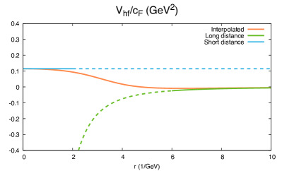
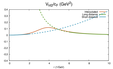
Figure 1: The two spin-dependent potentials (5) at short (13) [blue line] and long (III.2) [green line] distances. The orange line shows the interpolation we use (III.3). The short distance parameters $A$ and $B$ correspond to those in Table 3 and $r_{0}=3.96$ GeV^-1.

IV Charmonium Hybrids: fixing the short distance parameters

The short distance potentials depend on two arbitrary parameters at LO, $A$ and $B$. We shall fix those parameters by comparing our results to the lattice data of ref. Cheung:2016bym for the lower lying hybrid states (the $1(s/d)_{1}$ ($H_{1}$), $1p_{1}$ ($H_{2}$), $1(p/f)_{2}$ ($H_{4}$) and $1p_{0}$ ($H_{3}$) multiplets). The spin average of the multiplets in ref. Cheung:2016bym were higher than in ref. Oncala:2017hop . Since we are going to use the same methodology as in the last reference, we correct the lattice data by the spin average difference, namely by $381$ MeV ($1(s/d)_{1}$ ), $326$ MeV ($1p_{1}$), $392$ MeV ($1(p/f)_{2}$) and $151$ ($1p_{0}$) MeV. We then scan natural values of $A$ and $B$ in $[-0.3\,,0.3]$ GeV and $[-0.06\,,0.06]$ GeV³ respectively and search for the ones with the lowest $\chi^{2}/dof$. We adapted the code used in ref. Oncala:2017hop by adding the spin dependent potentials above, and neglecting, for simplicity, the mixing with quarkonium sandratfg . The charm mass is also taken as in ref. Oncala:2017hop , $m_{c}=1.47$ GeV. If we neglect the long distance behavior, we find $A=0.0699$ GeV, $B=0.0008$ GeV³ with $\chi^{2}/dof=1.1927$. When we include the long distance behavior the fit quality improves considerably, we obtain as a best fit $A=0.1356$ GeV, $B=-0.0022$ GeV³ with $\chi^{2}/dof=0,6439$. $g\Lambda^{\prime}$ and $g\Lambda^{\prime\prime\prime}$ are taken as in (15), $r_{0}=3.96$ GeV^-1 in (III.3) and all possible sign combinations for the long distance potentials in (III.2) and (15) are considered. The best fit corresponds to a negative $V_{ld}^{sa}(r)$ and a positive $V_{ld}^{sb}(r)$. The former implies $g\Lambda^{\prime\prime\prime}<0$. Reversing the sign of $V_{ld}^{sa}(r)$ ($V_{ld}^{sb}(r)$) worsens the fit considerably (marginally), see Table 1.

sign($V_{ld}^{sa}$) sign($V_{ld}^{sb}$)		$+-$	$++$	$-+$	$--$
$\chi^{2}/dof$		0.8323	0.7524	0.6439	0.6850
$A$ (GeV)		0.0764	0.0873	0.1356	0.1256
$B$ (GeV3)		0.0120	0.0144	-0.0022	-0.0045
$(s/d)_{1}$	$1^{--}$	4.0107	4.0107	4.0107	4.0107
mass	$0^{-+}$	3.9059	3.9029	3.8959	3.8988
(GeV)	$1^{-+}$	3.9582	3.9569	3.9548	3.9558
	$2^{-+}$	4.0597	4.0603	4.0612	4.0611
$p_{1}$ mass	$1^{++}$	4.1450	4.1450	4.1450	4.1450
(GeV)	$0^{+-}$	4.0886	4.0904	4.0981	4.0955
	$1^{+-}$	4.0880	4.0921	4.1020	4.0984
	$2^{+-}$	4.1456	4.1467	4.1495	4.1485
$(p/f)_{2}$	$2^{++}$	4.2316	4.2316	4.2316	4.2316
mass	$1^{+-}$	4.1963	4.1969	4.1959	4.1950
(GeV)	$2^{+-}$	4.2366	4.2343	4.2323	4.2343
	$3^{+-}$	4.2660	4.2637	4.2569	4.2594
$p_{0}$ mass	$0^{++}$	4.4864	4.4864	4.4864	4.4864
(GeV)	$1^{+-}$	4.4674	4.4693	4.4564	4.4554

Table 1: Fit parameters and spectrum dependence on the sign ambiguities arising from the long distance spin dependent potentials.

We have also explored the dependence of the result on $g\Lambda^{\prime}$ and $g\Lambda^{\prime\prime\prime}$ according to the possible values given in ref. Oncala:2017hop . The fit has a mild preference for larger values of $|g\Lambda^{\prime}|$ and $|g\Lambda^{\prime\prime\prime}|$ ($\chi^{2}/dof=0,632$ versus $\chi^{2}/dof=0,643$) , so we shall take for now on $g\Lambda^{\prime}=-0.0796$ GeV and $g\Lambda^{\prime\prime\prime}=0.3105$ GeV, which corresponds to the fit to long distance data only in ref. Oncala:2017hop . These values lead to $A=0.1445$ GeV and $B=-0.0036$ GeV³. The change in the spectrum is negligibly small ($\lesssim 1$ MeV). The interpolation dependence is estimated by moving $r_{0}\in[2.5\,,5]$ GeV^-1. The $\chi^{2}/dof$ marginally improves around $r_{0}\sim 3.5$ GeV^-1, and considerably deteriorates for $r_{0}\leq 3$ GeV^-1 and $r_{0}>3.96$ GeV^-1. We shall stick to the default value $r_{0}=3.96$ GeV^-1 and use $r_{0}\sim 3.5$ GeV^-1 to estimate the error due to the interpolation. The changes in the spectrum are of $3.1$ MeV in average, with a maximum of $7$ MeV. $A$ increases about a $30\%$ and $B$ becomes more than twice its value. See Table 2.

$r_{0}$ (Gev-1)		$2.5$	$3$	$3.5$	$3.96$	$5$
$\chi^{2}/dof$		1.0693	0.7088	0.6216	0.6318	0.7585
$A$ (GeV)		0.3718	0.2439	0.1793	0.1445	0.1049
$B$ (GeV3)		-0.0906	-0-0251	-0.0089	-0.0036	-0.0001
$(s/d)_{1}$	$1^{--}$	4.0107	4.0107	4.0107	4.0107	4.0107
mass	$0^{-+}$	3.8765	3.8836	3.8894	3.8945	3.9038
(GeV)	$1^{-+}$	3.9547	3.9525	3.9529	3.9543	3.9578
	$2^{-+}$	4.0438	4.0543	4.0593	4.0609	4.0604
$p_{1}$ mass	$1^{++}$	4.1450	4.1450	4.1450	4.1450	4.1450
(GeV)	$0^{+-}$	4.1122	4.1021	4.0991	4.0974	4.0946
	$1^{+-}$	4.1172	4.1174	4.1119	4.1045	4.0927
	$2^{+-}$	4.1559	4.1550	4.1524	4.1502	4.1471
$(p/f)_{2}$	$2^{++}$	4.2316	4.2316	4.2316	4.2316	4.2316
mass	$1^{+-}$	4.2291	4.2073	4.1975	4.1952	4.1958
(GeV)	$2^{+-}$	4.2334	4.2319	4.2320	4.2327	4.2349
	$3^{+-}$	4.2226	4.2366	4.2474	4.2545	4.2633
$p_{0}$ mass	$0^{++}$	4.4864	4.4864	4.4864	4.4864	4.4864
(GeV)	$1^{+-}$	4.4640	4.4558	4.4534	4.4546	4.4597

Table 2: Fit parameters and spectrum dependence on $r_{0}$.

In order to establish the error of $A$ and $B$ due to the input data, we assume a linear dependence of the binding energy on them, which holds at first order in perturbation theory. We obtain $A=0.115\pm 0.034$ GeV and $B=0.0038\pm 0.0154$ GeV³. Notice that the value of $B$ is compatible with zero. The spectrum is displayed in Table 3. The error due to the uncertainty in $g\Lambda^{\prime}$ and $g\Lambda^{\prime\prime\prime}$ is negligible. We also neglect the error due to the interpolation, which is not negligible in order to obtain a value for $A$ and $B$, but it is for the spectrum due to its correlation with $r0$. We include the error due to higher orders in the $1/m_{Q}$ expansion, which is about $30$ MeV for charm.

			Fit error	Total error
$A$ (GeV)		0.11455	0.034
$B$ (GeV3)		0.00385	0.0154
$(s/d)_{1}$	$1^{--}$	4.011		0.030
mass	$0^{-+}$	3.911	0.045	0.054
(GeV)	$1^{-+}$	3.963	0.023	0.038
	$2^{-+}$	4.046	0.018	0.035
$p_{1}$ mass	$1^{++}$	4.145		0.030
(GeV)	$0^{+-}$	4.087	0.054	0.061
	$1^{+-}$	4.055	0.023	0.037
	$2^{+-}$	4.130	0.005	0.030
$(p/f)_{2}$	$2^{++}$	4.232		0.030
mass	$1^{+-}$	4.235	0.019	0.035
(GeV)	$2^{+-}$	4.258	0.021	0.037
	$3^{+-}$	4.241	0.013	0.033
$p_{0}$ mass	$0^{++}$	4.486		0.030
(GeV)	$1^{+-}$	4.450	0.013	0.033

Table 3: Fit errors in $A$, $B$ and in the hybrid charmonium spectrum. The total errors in the spectrum are obtained by adding in quadrature the error due to missing higher orders in the $1/m_{Q}$ expansion ($\sim\Lambda_{\rm QCD}^{3}/m_{Q}^{2}\sim 30$ MeV).

In ref. Oncala:2017hop , it was found that two extra multiplets lie below the $1p_{0}$, the $2(s/d)_{2})$ and the $d_{2}$. For completeness we also display the spectrum of these multiplets including the hyperfine splitting in Table 4.

		Mass (GeV)	$A$ and $B$ error	Total error
$d_{2}$	$2^{--}$	4.486		0.030
	$1^{-+}$	4.287	${}_{-0.062}^{+0.050}$	${}_{-0.068}^{+0.059}$
	$2^{-+}$	4.302	${}_{-0.039}^{+0.031}$	${}_{-0.049}^{+0.043}$
	$3^{-+}$	4.333	${}_{-0.034}^{+0.003}$	${}_{-0.046}^{+0.030}$
$2(s/d)_{1}$	$1^{--}$	4.355		0.030
	$0^{-+}$	4.280	${}_{-0.066}^{+0.060}$	${}_{-0.072}^{+0.067}$
	$1^{-+}$	4.334	${}_{-0.006}^{+0.020}$	${}_{-0.031}^{+0.036}$
	$2^{-+}$	4.394	${}_{-0.032}^{+0.013}$	${}_{-0.044}^{+0.033}$

Table 4: The remaining hybrid charmonium spectrum below the $1p_{0}$ multiplet. The total errors in the spectrum are obtained by adding in quadrature to the errors induced by the uncertainties in $A$ and $B$ the error due to missing higher orders in the $1/m_{Q}$ expansion ($\sim\Lambda_{\rm QCD}^{3}/m_{Q}^{2}\sim 30$ MeV).

V Bottomonium Hybrids: predicting the hyperfine splittings

Once the parameters $A$ and $B$ are fixed from charmonium, the corresponding parameters for bottomonium, $A^{\prime}$ and $B^{\prime}$ also are,

$$A^{\prime}=A\frac{c_{F}(m_{b})m_{c}}{c_{F}(m_{c})m_{b}}\quad B^{\prime}=B\frac{c_{F}(m_{b})m_{c}}{c_{F}(m_{c})m_{b}}$$ (17)

We calculate the spectrum for the central values of these parameters ($A^{\prime}=0.02704$ GeV, $B^{\prime}=0.00091$ GeV³), which provides us with the central value of the masses, and for the four corners of their $1\,\sigma$ range, which allows us to estimate the error due to the fit parameters. We take it as the larger difference in either sense. The total error is obtained by adding in quadrature to the latter the error associated to higher orders $\sim\Lambda_{\rm QCD}^{3}/m_{Q}^{2}\sim 3$ MeV. The bottom mass is taken as in ref. Oncala:2017hop , $m_{b}=4.88$ GeV. We display the results in Table 5.

		Mass (GeV)	$A$ and $B$ error	Total error
$(s/d)_{1}$	$1^{--}$	10.6902		0.003
	$0^{-+}$	10.682	0.004	0.005
	$1^{-+}$	10.686	0.002	0.004
	$2^{-+}$	10.694	0.002	0.003
$p_{1}$	$1^{++}$	10.761		0.003
	$0^{+-}$	10.756	0.004	0.005
	$1^{+-}$	10.759	0.002	0.004
	$2^{+-}$	10.764	0.002	0.003
$(p/f)_{2}$	$2^{++}$	10.819		0.003
	$1^{+-}$	10.815	0.002	0.003
	$2^{+-}$	10.818	0.000	0.003
	$3^{+-}$	10.821	0.001	0.003
$d_{2}$	$2^{--}$	10.870		0.003
	$1^{-+}$	10.869	${}_{-0.003}^{+0.001}$	${}_{-0.005}^{+0.003}$
	$2^{-+}$	10.869	${}_{-0.002}^{+0.001}$	${}_{-0.004}^{+0.003}$
	$3^{-+}$	10.871	0.001	0.003
$2(s/d)_{1}$	$1^{--}$	10.885		0.003
	$0^{-+}$	10.881	${}_{-0.005}^{+0.002}$	${}_{-0.006}^{+0.004}$
	$1^{-+}$	10.883	${}_{-0.002}^{+0.001}$	0.003
	$2^{-+}$	10.888	${}_{-0.001}^{+0.003}$	${}_{-0.003}^{+0.004}$
$2p_{1}$	$1^{++}$	10.970		0.003
	$0^{+-}$	10.967	${}_{-0.004}^{+0.002}$	${}_{-0.004}^{+0.005}$
	$1^{+-}$	10.968	${}_{-0.001}^{+0.002}$	${}_{-0.003}^{+0.004}$
	$2^{+-}$	10.971	0.001	0.003
$2(p/f)_{2}$	$2^{++}$	11.005		0.003
	$1^{+-}$	11.003	${}_{-0.002}^{+0.001}$	0.003
	$2^{+-}$	11.005	0.000	0.003
	$3^{+-}$	11.007	0.001	$0.003$
$p_{0}$	$0^{++}$	11.012		0.003
	$1^{+-}$	11.012	0.000	0.003

Table 5: The hybrid bottomonium spectrum. The total errors in the spectrum are obtained by adding in quadrature to the fit errors the error due to missing higher orders in the $1/m_{Q}$ expansion ($\sim\Lambda_{\rm QCD}^{3}/m_{Q}^{2}\sim 3$ MeV).

We have also explored the dependence on $r_{0}$. We have recalculated the central values for $r_{0}=3.5$ GeV^-1 and the corresponding parameters (obtained from charm and converted to bottom according to (17), $A^{\prime}=0.0423$ GeV, $B^{\prime}=-0.0021$ GeV³). Recall that this $r_{0}$ choice provides a slightly better fit to charmonium lattice data than our default $r_{0}=3.96$ GeV^-1. The difference is below $1$ MeV for the $(s/d)_{1}$ multiplet and around $0.1$ MeV for the remaining ones. We can then safely neglect it.

VI Comparison with other approaches

We shall compare here our results with those also obtained in BOEFT in Refs. Brambilla:2018pyn ; Brambilla:2019jfi and with the lattice QCD results of the HSC collaboration Cheung:2016bym ; Ryan:2020iog (we will not use earlier results at larger pion masses HadronSpectrum:2012gic ). Recall that the main differences with respect to Refs. Brambilla:2018pyn ; Brambilla:2019jfi is that only short distance expressions for the spin-dependent potentials at NLO ($8$ non-perturbative parameters to fit) are used there, whereas we use LO short distance expressions and LO long distance expressions ($2$ non-perturbative parameters to fit).

Lattice results for charmonium hybrids Cheung:2016bym are used to fit the non-perturbative parameters. Hence, our errors are slightly larger than the ones from lattice data. Our fits have lower $\chi^{2}/{\rm dof}$ than those in Refs. Brambilla:2018pyn ; Brambilla:2019jfi , which supports the inclusion of long distance potentials. The overall picture for the charmonium hyperfine splittings is similar to the one obtained in those references, see Fig. 2. For spin one states we get similar, slightly larger, smaller and larger errors for the $(s/d)_{1}$ ($H_{1}$), $p_{1}$ ($H_{3}$), $(p/f)_{2}$ ($H_{4}$) and $p_{0}$ ($H_{3}$) multiplets respectively. For spin zero states, which do not enter in our analysis, the errors are only due to neglected higher orders in the $1/m_{Q}$ expansion. Note that the error that we assign to them is larger than than the one assigned in Refs. Brambilla:2018pyn ; Brambilla:2019jfi . See Fig. 2.

Our predictions for the bottomonium hybrid hyperfine splittings are compatible with the few available states from lattice QCD Ryan:2020iog , but we have much smaller errors, see Fig. 3. We get again an overall picture similar to the one of ref. Brambilla:2018pyn ; Brambilla:2019jfi , with smaller errors for spin one states, and smaller hyperfine splittings in general. However, for the $(s/d)_{1}$ multiplet we have about $2\sigma$ discrepancies with those references. Nevertheless, both sets of splittings are consistent with lattice data of Ryan:2020iog for this multiplet. The remaining available lattice states do not form any obvious spin multiplet. We have assigned the three lighter (two heavier) ones to the $p_{1}$ ($(p/f)_{2}$) multiplet. However, the fact that the $1^{++}$ state is lighter than the $1^{--}$ in the lattice results is in conflict with the BOEFT ones.

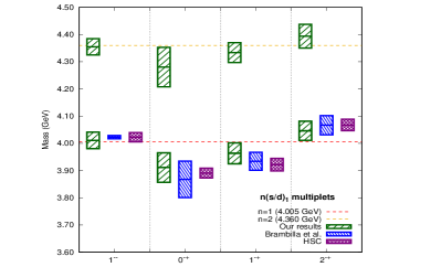
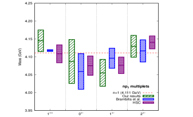
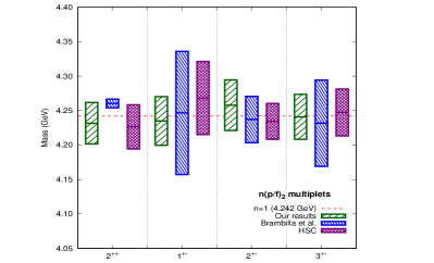
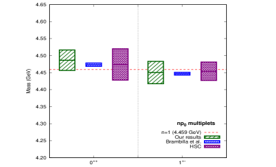
Figure 2: The spectrum of the lower-lying $n\,(s/d)_{1}$ ($H_{1}$), $n\,p_{1}$ ($H_{3}$), $n\,(p/f)_{2}$ ($H_{4}$) and $n\,p_{0}$ ($H_{3}$) charmonium hybrids computed by adding the LO spin-dependent potentials to the static potentials used in ref. Oncala:2017hop is shown in green boxes. The average mass for each multiplet is shown as a red dashed line. Blue and magenta boxes show the results of the BOEFT with NLO spin-dependent short distance potentials only Brambilla:2018pyn ; Brambilla:2019jfi and lattice QCD Cheung:2016bym respectively, adjusted to our spin average. The height of the boxes indicates the uncertainty.

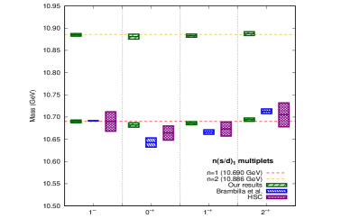
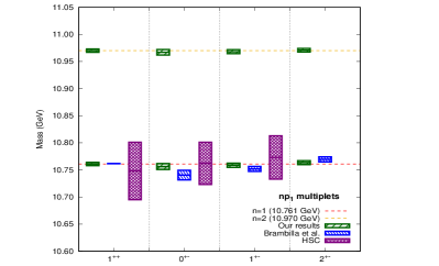
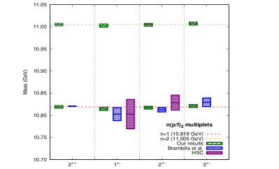
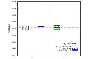
Figure 3: The spectrum of the lower-lying $n\,(s/d)_{1}$ ($H_{1}$), $n\,p_{1}$ ($H_{3}$), $n\,(p/f)_{2}$ ($H_{4}$) and $n\,p_{0}$ ($H_{3}$) bottommonium hybrids computed by adding the LO spin-dependent potentials to the static potentials used in ref. Oncala:2017hop is shown in green boxes. The average mass for each multiplet is shown as a red dashed line. Blue and magenta boxes show the results of the BOEFT with NLO spin-dependent short distance potentials only Brambilla:2018pyn ; Brambilla:2019jfi and lattice QCD Ryan:2020iog respectively, adjusted to our spin average. The height of the boxes indicates the uncertainty.

VII Discussion and Conclusions

The static potentials we use are taken from Oncala:2017hop . They were obtained from pure $SU(3)$ ($n_{f}=0$) lattice data of Refs. Juge:2002br ; Bali:2003jq . More recent pure $SU(3)$ ($n_{f}=0$) lattice data exist for the static hybrid potentials, with better resolution at short and intermediate distances Capitani:2018rox ; Muller:2019joq ; Schlosser:2021wnr . It would be interesting to incorporate it in future analysis. However, the systematic errors due to using pure $SU(3)$ ($n_{f}=0$) rather than QCD with dynamical light quarks ($n_{f}=3$) would still be difficult to evaluate. The early study of ref. Bali:2000vr suggest that they are small. The strategy recently presented in DallaBrida:2022eua may help to resolve this issue.

The lattice data to which we fit our spin-dependent expressions, ref. Cheung:2016bym , is obtained from a $2+1+1$ clover action at a fixed spacial lattice spacing of $0.12$ fm, a $3.5$ times smaller temporal lattice spacing, and light quark masses corresponding to $m_{\pi}\sim 240$ MeV. In ref. Ray:2021nhe results in the continuum limit for realistic light quark masses are obtained using a HISQ action with $2+1+1$ dynamical quarks, but only for two states in the lowest lying multiplet. The lattice bottomonium data we compare with, ref. Ryan:2020iog , uses the same setting as Cheung:2016bym , tuning the heavy quark parameters to bottomonium observables, and uses light quark masses corresponding to $m_{\pi}\sim 391$ MeV.

We have focused on the hyperfine splittings. The absolute values of the masses we quote correspond to the spin averages of Ref. Oncala:2017hop . The central values quoted in that reference are lower than those in Ref. Berwein:2015vca but compatible within errors. The differences are due to the choice of normalization (quarkonium spectrum versus RS mass scheme). They are also much lower than the lattice results of Ref. Cheung:2016bym , a difference that shrinks if they are compared with earlier lattice data at larger pion mass HadronSpectrum:2012gic . This suggest that part of the discrepancy may be due to the quenched lattice data used as an input in Refs. Berwein:2015vca ; Oncala:2017hop . They are also lower than in most models (see Meyer:2015eta for a review). Since the discrepancies usually amount to global shifts, they are not expected to affect the bulk of the hyperfine splitting analysis presented here. However, a small dependence on the input lattice data (unphysical) pion mass was noticed in the short distance analysis of Ref. Brambilla:2019jfi , which may be present in our results as well.

We have shown that the inclusion of long distance contributions calculated in the QCD EST to the LO spin dependent potentials in the BOEFT considerable improves the description of the charmonium hybrids hyperfine splittings obtained in lattice QCD Cheung:2016bym . For the LO spin-dependent potentials the $\chi^{2}/dof$ moves from $1.193$ for short distance contributions only to $0.644$ for short and long distance contributions. This figure is much lower than the $\chi^{2}/dof=0.999$ obtained in ref. Brambilla:2019jfi for NLO spin-dependent potential with short distance contributions only. The fact that long distance contributions are important may be anticipated from the results on the size of charmonium hybrids displayed in Table III of ref. Berwein:2015vca , $\langle 1/r\rangle\in\left[190,420\right]$ MeV, scales of the order of $\Lambda_{\rm QCD}$. Using the QCD EST to describe them has the remarkable feature that it introduces no new unknown parameter, beyond sign ambiguities and the scale $r_{0}$ that separates short and long distances in the interpolation. Hence we have two parameter fits to data, rather than the eight parameter fits of ref. Brambilla:2019jfi , leading to a smaller $\chi^{2}/dof$ as mentioned above.

Once we have the unknown parameters fixed, we can calculate the hyperfine splittings of higher charmonium hybrid states, of the bottomonium ones, and the error associated to them. This is displayed in Tables 3, 4 and 5 and in Figs. 2 and 3. For charmonium hybrids, we get results compatible with ref. Brambilla:2019jfi with similar errors overall, and, as expected, compatible with ref. Cheung:2016bym , the source of our fit, with slightly larger errors. For bottomonium hybrids our hyperfine splittings are compatible with those of Ref. Ryan:2020iog , with much smaller errors, but smaller than those in Ref. Brambilla:2019jfi , with similar errors.

Appendix A Effective string theory calculation

The general expressions for the (heavy quark) spin dependent potentials (1), given in Ref. Soto:2020xpm , reduce for $\kappa^{p}=1^{+}$ to

$$\frac{V^{sa}_{1^{+}11}(r)}{m_{Q}} = \lim_{T\to\infty}\frac{g\,c_{F}}{m_{Q}T}\int_{-\frac{T}{2}}^{\frac{T}{2}}dt\frac{\langle B^{\ast}({\bf 0},\frac{T}{2}){B^{3}}(\frac{\bf r}{2},t){B}({\bf 0},-\frac{T}{2})-B({\bf 0},\frac{T}{2}){B^{3}}(\frac{\bf r}{2},t){B^{\ast}}({\bf 0},-\frac{T}{2})\rangle_{\Box}}{\langle{B}({\bf 0},\frac{T}{2}){B^{\ast}}({\bf 0},-\frac{T}{2})+{B^{\ast}}({\bf 0},\frac{T}{2}){B}({\bf 0},-\frac{T}{2})\rangle_{\Box}}$$ (18)

$$\frac{V^{sb}_{1^{+}10}(r)}{m_{Q}} = \lim_{T\to\infty}\frac{g\,c_{F}}{4m_{Q}}\frac{V_{\Pi_{u}}-V_{\Sigma_{u}^{-}}}{\sin\left((V_{\Pi_{u}}-V_{\Sigma_{u}^{-}})\frac{T}{2}\right)}\int_{-\frac{T}{2}}^{\frac{T}{2}}dt\frac{\langle\left(B^{\ast}({\bf 0},\frac{T}{2}){B}(\frac{\bf r}{2},t)-B({\bf 0},\frac{T}{2}){B^{\ast}}(\frac{\bf r}{2},t)\right){B^{3}}({\bf 0},-\frac{T}{2})\rangle_{\Box}}{\langle{B}({\bf 0},\frac{T}{2}){B^{\ast}}({\bf 0},-\frac{T}{2})+{B^{\ast}}({\bf 0},\frac{T}{2}){B}({\bf 0},-\frac{T}{2})\rangle_{\Box}^{1/2}\langle{B^{3}}({\bf 0},\frac{T}{2}){B^{3}}({\bf 0},-\frac{T}{2})\rangle_{\Box}^{1/2}}$$

where ${B^{i}}({\bf r},t)$, $i=1,2,3$ are the three components of the chromomagnetic field, and

$$B({\bf r},t) = B^{1}({\bf r},t)+iB^{2}({\bf r},t)$$ (19)

$$B^{\ast}({\bf r},t) = B^{1}({\bf r},t)-iB^{2}({\bf r},t)\,.$$

${\bf{\hat{r}}}$ is taken in the $z$ direction. The mapping of the operator insertions in the temporal Wilson lines onto EST operators was given in Perez-Nadal:2008wtr ,

$$B(\pm{\bf r}/2,t) \rightarrow -i\sqrt{2}\Lambda^{\prime}\partial_{t}\partial_{z}\varphi(\pm r/2,t)$$

$$B^{\ast}(\pm{\bf r}/2,t) \rightarrow i\sqrt{2}\Lambda^{\prime}\partial_{t}\partial_{z}\varphi^{\ast}(\pm r/2,t)$$ (20)

$$B^{3}(\pm{\bf r}/2,t) \rightarrow i\Lambda^{\prime\prime\prime}\partial_{t}\partial_{z}\varphi(\pm r/2,t)\partial_{z}\varphi^{\ast}(\pm r/2,t)+{\rm H.c.}\,,$$

and the mapping of the operator insertions in the middle of spacial Wilson lines at $t=\pm T/2$ onto string states in Oncala:2017hop ,

$${B}({\bf 0},t) \to \pm i{\tilde{\Lambda}}^{2}\partial_{0}\varphi({0},t)$$

$${B^{\ast}}({\bf 0},t) \to \mp i{\tilde{\Lambda}}^{2}\partial_{0}\varphi^{\ast}({0},t)$$ (21)

$${B^{3}}({\bf 0},t) \to \pm{\tilde{\Lambda}}^{\prime 2}i\partial_{0}\varphi({0},t)\partial_{z}\varphi^{\ast}({0},t)+{\rm H.c.}\,,$$

$t=\pm\frac{T}{2}$. Note that neither $V^{sa}_{1^{+}11}(r)$ nor $V^{sb}_{1^{+}11}(r)$ depend on the values of ${\tilde{\Lambda}}^{2}$ or ${\tilde{\Lambda}}^{\prime 2}$. $V^{sa}_{1^{+}11}(r)$ is not sensitive to the sign ambiguity of the mapping either, however $V^{sb}_{1^{+}10}(r)$ is, which produces a sign ambiguity in it. Recall that $V_{\Pi_{u}}-V_{\Sigma_{u}^{-}}=-\frac{2\pi}{r}$ in EST. Once these substitutions are carried out in (18), and the QCD vacuum averages $\langle\dots\rangle_{\Box}$ replaced by the string vacuum average $\langle\dots\rangle$, a simple (tree level) calculation in EST leads to (III.2) javier .

References

- (1) R. L. Jaffe and K. Johnson, Phys. Lett. B 60, 201-204 (1976) doi:10.1016/0370-2693(76)90423-8
- (2) E. Braaten, C. Langmack and D. H. Smith, Phys. Rev. D 90, no.1, 014044 (2014) doi:10.1103/PhysRevD.90.014044 [arXiv:1402.0438 [hep-ph]].
- (3) M. Berwein, N. Brambilla, J. Tarrús Castellà and A. Vairo, Phys. Rev. D 92, no.11, 114019 (2015) doi:10.1103/PhysRevD.92.114019 [arXiv:1510.04299 [hep-ph]].
- (4) R. Oncala and J. Soto, Phys. Rev. D 96, no.1, 014004 (2017) doi:10.1103/PhysRevD.96.014004 [arXiv:1702.03900 [hep-ph]].
- (5) J. Soto, Nucl. Part. Phys. Proc. 294-296, 87-94 (2018) doi:10.1016/j.nuclphysbps.2018.03.020 [arXiv:1709.08038 [hep-ph]].
- (6) N. Brambilla, W. K. Lai, J. Segovia, J. Tarrús Castellà and A. Vairo, Phys. Rev. D 99, no.1, 014017 (2019) [erratum: Phys. Rev. D 101, no.9, 099902 (2020)] doi:10.1103/PhysRevD.99.014017 [arXiv:1805.07713 [hep-ph]].
- (7) J. Soto and J. Tarrús Castellà, Phys. Rev. D 102, no.1, 014012 (2020) doi:10.1103/PhysRevD.102.014012 [arXiv:2005.00552 [hep-ph]].
- (8) K. J. Juge, J. Kuti and C. J. Morningstar, Phys. Rev. Lett. 82, 4400-4403 (1999) doi:10.1103/PhysRevLett.82.4400 [arXiv:hep-ph/9902336 [hep-ph]].
- (9) E. Braaten, C. Langmack and D. H. Smith, Phys. Rev. Lett. 112, 222001 (2014) doi:10.1103/PhysRevLett.112.222001 [arXiv:1401.7351 [hep-ph]].
- (10) J. Tarrús Castellà and E. Passemar, Phys. Rev. D 104, no.3, 034019 (2021) doi:10.1103/PhysRevD.104.034019 [arXiv:2104.03975 [hep-ph]].
- (11) N. Brambilla, W. K. Lai, A. Mohapatra and A. Vairo, [arXiv:2212.09187 [hep-ph]].
- (12) A. Pineda and J. Tarrús Castellà, Phys. Rev. D 100, no.5, 054021 (2019) doi:10.1103/PhysRevD.100.054021 [arXiv:1905.03794 [hep-ph]].
- (13) N. Brambilla, S. Eidelman, C. Hanhart, A. Nefediev, C. P. Shen, C. E. Thomas, A. Vairo and C. Z. Yuan, Phys. Rept. 873, 1-154 (2020) doi:10.1016/j.physrep.2020.05.001 [arXiv:1907.07583 [hep-ex]].
- (14) H. X. Chen, W. Chen, X. Liu, Y. R. Liu and S. L. Zhu, Rept. Prog. Phys. 86, no.2, 026201 (2023) doi:10.1088/1361-6633/aca3b6 [arXiv:2204.02649 [hep-ph]].
- (15) N. Brambilla, W. K. Lai, J. Segovia and J. Tarrús Castellà, Phys. Rev. D 101, no.5, 054040 (2020) doi:10.1103/PhysRevD.101.054040 [arXiv:1908.11699 [hep-ph]].
- (16) M. Luscher and P. Weisz, JHEP 07, 049 (2002) doi:10.1088/1126-6708/2002/07/049 [arXiv:hep-lat/0207003 [hep-lat]].
- (17) M. Luscher and P. Weisz, JHEP 07, 014 (2004) doi:10.1088/1126-6708/2004/07/014 [arXiv:hep-th/0406205 [hep-th]].
- (18) G. Perez-Nadal and J. Soto, Phys. Rev. D 79, 114002 (2009) doi:10.1103/PhysRevD.79.114002 [arXiv:0811.2762 [hep-ph]].
- (19) N. Brambilla, M. Groher, H. E. Martinez and A. Vairo, Phys. Rev. D 90, no.11, 114032 (2014) doi:10.1103/PhysRevD.90.114032 [arXiv:1407.7761 [hep-ph]].
- (20) G. K. C. Cheung et al. [Hadron Spectrum], JHEP 12, 089 (2016) doi:10.1007/JHEP12(2016)089 [arXiv:1610.01073 [hep-lat]].
- (21) J. Tarrús Castellà, AIP Conf. Proc. 2249, no.1, 020008 (2020) doi:10.1063/5.0008570 [arXiv:1908.05179 [hep-ph]].
- (22) P. Solé Campreciós, “Heavy Hybrids Mesons in NRQCD: Fine and Hyperfine Structure,” Bachelor Thesis, Universitat de Barcelona (June 2017)
- (23) P. Molina Grífols, “Spin-dependent Effects on the Hyperfine Structure in Heavy Hybrid Mesons,” Bachelor Thesis, Universitat de Barcelona (February 2021)
- (24) A. Pineda and J. Soto, Nucl. Phys. B Proc. Suppl. 64, 428-432 (1998) doi:10.1016/S0920-5632(97)01102-X [arXiv:hep-ph/9707481 [hep-ph]].
- (25) N. Brambilla, A. Pineda, J. Soto and A. Vairo, Nucl. Phys. B 566, 275 (2000) doi:10.1016/S0550-3213(99)00693-8 [arXiv:hep-ph/9907240 [hep-ph]].
- (26) K. J. Juge, J. Kuti and C. Morningstar, Phys. Rev. Lett. 90, 161601 (2003) doi:10.1103/PhysRevLett.90.161601 [arXiv:hep-lat/0207004 [hep-lat]].
- (27) G. S. Bali and A. Pineda, Phys. Rev. D 69, 094001 (2004) doi:10.1103/PhysRevD.69.094001 [arXiv:hep-ph/0310130 [hep-ph]].
- (28) S. Capitani, O. Philipsen, C. Reisinger, C. Riehl and M. Wagner, Phys. Rev. D 99, no.3, 034502 (2019) doi:10.1103/PhysRevD.99.034502 [arXiv:1811.11046 [hep-lat]].
- (29) C. Schlosser and M. Wagner, Phys. Rev. D 105, no.5, 054503 (2022) doi:10.1103/PhysRevD.105.054503 [arXiv:2111.00741 [hep-lat]].
- (30) M. Luscher, K. Symanzik and P. Weisz, Nucl. Phys. B 173, 365 (1980) doi:10.1016/0550-3213(80)90009-7
- (31) A. V. Manohar, Phys. Rev. D 56, 230-237 (1997) doi:10.1103/PhysRevD.56.230 [arXiv:hep-ph/9701294 [hep-ph]].
- (32) G. Amoros, M. Beneke and M. Neubert, Phys. Lett. B 401, 81-90 (1997) doi:10.1016/S0370-2693(97)00345-6 [arXiv:hep-ph/9701375 [hep-ph]].
- (33) A. G. Grozin, P. Marquard, J. H. Piclum and M. Steinhauser, Nucl. Phys. B 789, 277-293 (2008) doi:10.1016/j.nuclphysb.2007.08.012 [arXiv:0707.1388 [hep-ph]].
- (34) J. Castillo Uviña, “Spin Dependent Potential of the Heavy Hybird Mesons,” Bachelor Thesis, Universitat de Barcelona (January 2020)
- (35) Y. Koma and M. Koma, PoS LAT2009, 122 (2009) doi:10.22323/1.091.0122 [arXiv:0911.3204 [hep-lat]].
- (36) Y. Koma and M. Koma, Nucl. Phys. B 769, 79-107 (2007) doi:10.1016/j.nuclphysb.2007.01.033 [arXiv:hep-lat/0609078 [hep-lat]].
- (37) S. Tomàs Valls, “Spectrum of heavy quarkonium hybrids: hyperfine splitting,” Bachelor Thesis, Universitat de Barcelona (January 2021)
- (38) S. M. Ryan et al. [Hadron Spectrum], JHEP 02, 214 (2021) doi:10.1007/JHEP02(2021)214 [arXiv:2008.02656 [hep-lat]].
- (39) L. Liu et al. [Hadron Spectrum], JHEP 07, 126 (2012) doi:10.1007/JHEP07(2012)126 [arXiv:1204.5425 [hep-ph]].
- (40) L. Müller, O. Philipsen, C. Reisinger and M. Wagner, Phys. Rev. D 100, no.5, 054503 (2019) doi:10.1103/PhysRevD.100.054503 [arXiv:1907.01482 [hep-lat]].
- (41) G. S. Bali et al. [TXL and T(X)L], Phys. Rev. D 62, 054503 (2000) doi:10.1103/PhysRevD.62.054503 [arXiv:hep-lat/0003012 [hep-lat]].
- (42) M. Dalla Brida et al. [ALPHA], Eur. Phys. J. C 82, no.12, 1092 (2022) doi:10.1140/epjc/s10052-022-10998-3 [arXiv:2209.14204 [hep-lat]].
- (43) G. Ray and C. McNeile, PoS LATTICE2021, 240 (2022) doi:10.22323/1.396.0240 [arXiv:2110.14101 [hep-lat]].
- (44) C. A. Meyer and E. S. Swanson, Prog. Part. Nucl. Phys. 82, 21-58 (2015) doi:10.1016/j.ppnp.2015.03.001 [arXiv:1502.07276 [hep-ph]].