AIROGS: Artificial Intelligence for RObust Glaucoma Screening Challenge

Abstract

The early detection of glaucoma is essential in preventing visual impairment. Artificial intelligence (AI) can be used to analyze color fundus photographs (CFPs) in a cost-effective manner, making glaucoma screening more accessible. While AI models for glaucoma screening from CFPs have shown promising results in laboratory settings, their performance decreases significantly in real-world scenarios due to the presence of out-of-distribution and low-quality images. To address this issue, we propose the Artificial Intelligence for Robust Glaucoma Screening (AIROGS) challenge. This challenge includes a large dataset of around 113,000 images from about 60,000 patients and 500 different screening centers, and encourages the development of algorithms that are robust to ungradable and unexpected input data. We evaluated solutions from 14 teams in this paper, and found that the best teams performed similarly to a set of 20 expert ophthalmologists and optometrists. The highest-scoring team achieved an area under the receiver operating characteristic curve of 0.99 (95% CI: 0.98-0.99) for detecting ungradable images on-the-fly. Additionally, many of the algorithms showed robust performance when tested on three other publicly available datasets. These results demonstrate the feasibility of robust AI-enabled glaucoma screening.

Keywords color fundus photography  $\cdot$ glaucoma screening  $\cdot$ out-of-distribution detection  $\cdot$ retina  $\cdot$ robustness

1 Introduction

Glaucoma is one of the main causes of irreversible blindness and impaired vision in the world. It affects the optic nerve, which connects the eye with the brain, and leads to progressive visual field damage. This damage initially passes unnoticed by the patient. Only in later stages will glaucoma patients experience visual loss. According to estimates, by 2040, over 110 million people will have varying degrees of visual impairment caused by glaucoma [1], with 10% becoming blind in both eyes and 25% in one eye [2]. Many people experience visual impairment from glaucoma because it is often not detected until later stages [3, 4]. Current treatments of glaucoma cannot repair the damage, but can only halt or slow the progression of the condition [5]. Implementing screening programs to identify patients early on for treatment can alleviate the consequences of the disease. Artificial intelligence (AI) may be the enabling technology for the cost-effective implementation of these programs by automatically detecting perimetric glaucoma (i.e., glaucoma in which there is already visual field damage) in color fundus photographs (CFPs) [6, 7, 8, 9, 10].

Table 1: Statistics of the Rotterdam EyePACS AIROGS dataset. # = number of. CFPs = color fundus photographs.

			Full set	Training set	Test set
# CFPs / # patients			112,732 / 60,071	101,442 / 54,274	11,290 / 5,797
Prevalence (# CFPs (% within set) / # patients)		RG	4,872 (4.3%) / 3,531	3,270 (3.2%) / 2,336	1,602 (14.2%) / 1,195
		NRG	106,306 (94.3%) / 58,388	98,172 (96.8%) / 53,400	8,134 (72.0%) / 4,988
		U	1,554 (1.4%) / 1,415	0 (0.0%) / 0	1,554 (13.8%) / 1,415
Age at encounter (mean $\pm$ std. dev.)			56.9 $\pm$ 10.3	56.7 $\pm$ 10.2	59.3 $\pm$ 10.9
# sites			500	486	376
Cameras (# CFPs (% within set) / # patients)	Canon	CR1	11,462 (10.2%) / 6,013	10,274 (10.1%) / 5,422	1,188 (10.5%) / 591
	Canon	CR2	10,523 (9.3%) / 5,538	9,179 (9.0%) / 4,866	1,344 (11.9%) / 672
	Canon	DGI	10,644 (9.4%) / 5,690	9,581 (9.4%) / 5,145	1,063 (9.4%) / 545
	Optovue	iCam 100	29,108 (25.8%) / 16,166	26,480 (26.1%) / 14,742	2,628 (23.3%) / 1,424
	TopCon	NW200	3,109 (2.8%) / 1,588	2,888 (2.8%) / 1,478	221 (2.0%) / 110
	TopCon	NW400	22,519 (20.0%) / 11,736	20,557 (20.3%) / 10,737	1,962 (17.4%) / 999
	Centervue	DRS	1,805 (1.6%) / 988	1,598 (1.6%) / 879	207 (1.8%) / 109
	Nidek	AFC300	61 (0.1%) / 31	53 (0.1%) / 27	8 (0.1%) / 4
	Crystalvue	NFC-700	8 (0.0%) / 4	6 (0.0%) / 3	2 (0.0%) / 1
	Unknown		23,493 (20.8%) / 12,323	20,826 (20.5%) / 10,981	2,667 (23.6%) / 1,342

Existing AI solutions have been shown to drop in performance in real-world screening practice due to comorbidities, poor quality images, different ethnicities, or unexpected out-of-distribution (OOD) samples [9]. Ad-hoc quality check modules have been added on AI solutions to overcome this performance drop, but recent research has indicated that these quality checks are not sufficiently accurate when deployed in real-world settings [11]. To allow a safe and effective deployment in screening, the reliability and robustness of such solutions need to be assessed. Medical image analysis challenges often exclusively focuses on performance metrics that are potentially unrealistic and overestimated due to the use of test sets that do not represent real-world scenarios. Moreover, metrics to measure reliability and robustness are often neglected due to the difficulty to estimate them in the provided test sets.

With the aim to develop solutions that overcome the aforementioned issues related to robustness in glaucoma screening, we organized the Artificial Intelligence for RObust Glaucoma Screening (AIROGS) challenge. The goal of this challenge was to evaluate the feasibility of the development of a state-of-the-art, reliable AI solution that takes a CFP as input and provides as output the likelihood of referable glaucoma, accompanied with outputs for robustness (i.e., predicting whether the input image can be graded reliably or not).

To encourage the development of solutions that are robust to any kind of ungradable and unexpected input data and are equipped with inherent robustness mechanisms, the training set we provided was a subset of the full AIROGS dataset where only gradable images were included and ungradable images excluded. The test set, however, is unfiltered, containing all images found in screening settings (gradable and ungradable), representing a real-world scenario.

AIROGS was part of the International Symposium on Biomedical Imaging (ISBI) 2022 challenge program. It reopened after presenting the results during ISBI 2022 and submissions can still be made on Grand Challenge.

Our challenge, along with the dataset we made publicly available, distinguishes itself from previous glaucoma challenges. First, to the best of our knowledge, our dataset is the largest publicly available CFP dataset with glaucoma labels by a large margin. In total, our dataset contains 112,732 CFPs, exceeding the size of other publicly available datasets containing CFPs with glaucoma, of which the sizes range from 22 to 2,000 CFPs [12, 13, 14, 15, 16, 17, 18, 19, 20]. It is a highly diverse dataset as it originates from 500 screening centers across the United States of America and was acquired with a large variety of cameras. Second, the AIROGS challenge is the first challenge to emphasize robustness in glaucoma screening. Third, AIROGS is one of the first type of challenges on grand-challenge.org that requires participants to submit an algorithm (a Type 2 challenge), rather than a file with their predictions on the test set (a Type 1 challenge), as is done in more traditional challenges. This makes human intervention in the generation of test set results impossible, reducing the possibility of cheating. Morever, it greatly improves reproducibility, allowing everyone to reuse the trained algorithms that were submitted and apply them to new data in a cloud-based environment. Fourth, the reproducibility enabled testing of the participating algorithms on three external datasets: two for evaluating the screening task and one for evaluating robustness.

2 Datasets

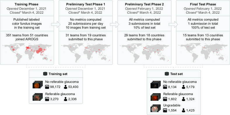
Figure 1: Overview of all phases in the AIROGS challenge. A world map is shown for each phase that indicates with red circles from which countries the teams that participated in that phase originated. A circle is shown for each country from which at least one team participated and its size represents the number of teams that joined from that country. The relevant subset of the AIROGS dataset for each phase is shown at the bottom of the figure. *All phases reopened for new submissions after the winning teams were announced.

2.1 The Rotterdam EyePACS AIROGS dataset

The Rotterdam EyePACS AIROGS dataset contains 112,732 CFPs from 60,071 subjects and 500 different sites with a heterogeneous ethnicity. The images were originally acquired for a diabetic retinopathy screening program [21]. For grading of the CFPs, all graders were trained and then selected for this task using the European Optic Disc Assessment Trial (EODAT) [22], containing 110 steroscopic optic nerve photographs, in which all glaucomatous eyes had reproducible visual field defects on standard automated perimetry. 90 experienced ophthalmologists and optometrists were examined and those who scored at least 85% overall accuracy and 92% specificity were selected to label images for the present study. Eventually, 30 out of 90 candidates passed.

For each eye, three images were taken by the camera operators to reduce the number of ungradable eyes. When labeling the images, graders classified one eye at a time. The labeling tool first presented the first CFP for each eye, upon when graders could choose from the options "Referable glaucoma" (RG), "No referable glaucoma" (NRG) or "Ungradable" (U). If a grader selected U for the first image, the tool showed the consecutive CFP. The third image was presented if the second image was also deemed U. Each eye was scored by two separate graders, who were both unaware about the identity of the other grader. If the two graders agreed on the label of a CFP, this became the final label. If they disagreed, the image was scored by one of the glaucoma specialists who passed the EODAT test with at least 95% accuracy. The final label was then based on his judgement.

The graders were instructed to select RG if they found glaucomatous signs which they expected to be associated with visual field defects on standard automated perimetry. The signs that could be selected were "appearance neuroretinal rim superiorly", "appearance neuroretinal rim inferiorly", "baring of the circumlinear vessel superiorly", "baring of the circumlinear vessel inferiorly", "disc hemorrhage(s)", "retinal nerve fibre layer defect superiorly", "retinal nerve fibre layer defect inferiorly", "nasalisation (nasal displacement) of the vessel trunk", "laminar dots" and "large cup". If the graders did not expect any glaucomatous visual field defects, NRG was to be selected, ignoring comorbidities such as age-related macular degeneration and diabetic retinopathy. If there was not enough information visible in the CFP to decide between RG and NRG, graders were instructed to select U.

The graders were not only evaluated at the start, but they were periodically monitored during the grading process, as well. If their sensitivity or specificity dropped below 80% or 95%, respectively, they were removed from the study and all images they labeled were re-graded by any of the remaining graders. In case a grader wrongly classified a CFP as U, while its final label was NRG or RG, their specificity or sensitivity went down, respectively. In the end, 20 graders remained.

Out of the three CFPs that were available for each eye, we only included the RG or NRG photograph in the dataset if it was available. Otherwise, only one of the U photographs was used. We split the data into a training set of 101,442 CFPs and a test set of 11,290 CFPs, ensuring that data from patients in the training set was not in the test set. We randomly sampled patients when making the split, oversampling patients with ungradable and RG CFPs for the test set, such that approximately 1,600 RG and 1,600 U photographs ended up in the test set. Since we were interested in AI solutions that can identify ungradable data without training on ungradable data, we left out all U photographs that ended up in the AIROGS training set. Table 1 shows statistics about RG, NRG and U prevalence, age, sites and cameras for the full dataset, the training set and the test set. Approval from the Institutional Review Board of the Rotterdam Eye Hospital was obtained to conduct this research.

2.2 External datasets

The participants uploaded their trained algorithms, rather than a file with predictions on our test set, to our challenge platform. This enabled us to reuse the developed models on external data after the challenge ended. To evaluate model generalization and to demonstrate this reusability, we applied all trained algorithms to three external datasets: Retinal Fundus Glaucoma Challenge (REFUGE) [18], Glaucoma grAding from Multi-Modality imAges (GAMMA) [20] and Diabetic Retinopathy Image Database (DRIMDB) [23]. The former two are datasets with positive and negative glaucoma CFPs, which we used for externally evaluating the screening performance. We used the latter dataset, which contained different types of ungradable images, to externally evaluate the robustness.

The REFUGE test set contained 400 CFPs, of which 40 CFPs showed glaucoma and 360 CFPs did not. The definition of glaucoma was glaucomatous damage in the optic nerve head area and reproducible glaucomatous visual field defects, which is similar to our definition of glaucoma described earlier [18].

The GAMMA dataset is a multi-modal dataset with optical coherence tomography scans and CFPs for each eye. We used the CFP data from the 100-sample training set as only that subset of the GAMMA dataset had publicly available labels. We defined positive glaucoma as the union of the intermediate and advanced glaucoma stages. These stages were defined using the mean deviation (MD) from the visual field reports as follows: an MD between than -6 dB and -12 dB for the intermediate stage and an MD worse than -12 dB for the advanced stage [20]. This resulted in 50 negative and 50 positive glaucoma samples.

DRIMDB is a dataset with 125 "Good" CFPs, 69 "Bad" CFPs and 22 "Outlier" CFPs. As the "Good" class was not necessarily defined as gradable for glaucoma, we manually confirmed that in all "Good" CFPs the optic disc (OD) was well visible. We defined both "Bad" and "Outlier" classes to be ungradable and the "Good" class to be gradable. "Bad" images were CFPs with low image quality and "Outlier" images were non-retinal images.

3 Challenge setup

The AIROGS challenge consisted of four phases (see Fig. 1). The Training Phase opened on the 1^st of December 2021 and closed on the 4^th of March 2022, providing the participants with approximately three months to develop their solutions. At the start of this phase, the training set was released and has since been available for download under the CC BY-NC-ND licence on Zenodo.

To ensure fair competition and to encourage the development of inherent robustness mechanisms, teams were not permitted to use additional fundus image training data, including weights pre-trained on fundus image data or in pre-processing steps such as OD segmentation. Manually labeling the challenge data and using the resulting annotations during training was allowed.

To test the algorithms developed by participants, they needed to wrap their trained algorithm in a Docker container and submit it to our challenge platform. This allows the submitted algorithms to be run on data that is not directly accessible by the participating teams. Example code for generating such a containerized submission can be found on GitHub. Preliminary Test Phase 1 opened and closed simultaneously with the Training phase and served as a check for whether the submitted algorithms could be run on the challenge platform and produced the output in the expected format. Algorithms were tested on 10 images from the training set for this check. All algorithms were executed on the challenge platform using an NVIDIA T4 GPU (16 GB VRAM) with 8 CPUs (32 GB RAM).

The test set was and still is closed, meaning the image data and the labels are private and cannot be downloaded. Preliminary Test Phase 2 opened on the 1^st of February 2022 and we allowed three submissions per team to this phase, as it used 10% of the test set for evaluation. All challenge metrics were also computed and reported back to the participants. The Final Test Phase opened simultaneously with Preliminary Test Phase 2, but algorithms were tested on 100% of the test data and only one submission per team was allowed. The challenge metrics computed for this phase were used for the final team ranking.

The algorithms were expected to produce four outputs, of which two were related to glaucoma screening performance (i.e., image classification of RG and NRG) and the other two to robustness (i.e., the identification of U). The glaucoma screening outputs were a likelihood score for RG ($O_{1}$) and a binary decision for RG ($O_{2}$, positive if RG and negative if NRG). The ungradability outputs were a binary decision on whether the image is ungradable ($O_{3}$, positive if ungradable and negative if ungradable) and a non-thresholded scalar value that is positively correlated with the likelihood for ungradability (e.g. the entropy of a probability vector produced by a machine learning model or the variance of an ensemble) ($O_{4}$). Output $O_{2}$ was not used in the evaluation pipeline for the challenge leaderboard, but it was requested by the challenge organizers for further analysis.

The evaluation was also based on the two aspects of screening performance and robustness, with two metrics per aspect. Screening performance was evaluated using the standardized partial area under the receiver operating characteristic curve [24] (90-100% specificity) for RG ($pAUC_{S}$), and the sensitivity at 95% specificity ($SE@95SP_{S}$). These metrics were based on these specificity ranges, as a high specificity is required for cost-effective glaucoma screening due to its relatively low prevalence [25, 26]. $pAUC_{S}$ and $SE@95SP_{S}$ are both based on output $O_{1}$. For evaluating the robustness, we determined the model’s agreement with the human reference on ungradability using Cohen’s kappa score ($\kappa_{U}$), calculated using output $O_{3}$. Furthermore, we calculated the area under the receiver operator characteristic curve using the human reference for ungradability as the true labels and output $O_{4}$ as the target scores ($AUC_{U}$).

To determine the final ranking, we first ranked all participants on the four individual metrics $pAUC_{S}$, $SE@95SP_{S}$, $\kappa_{U}$, and $AUC_{U}$ resulting in the rankings $R_{pAUC_{S}}$, $R_{SE@95SP_{S}}$, $R_{\kappa_{U}}$, and $R_{AUC_{U}}$, respectively. The final score $S_{final}$ was then calculated as the mean of those ranking:

$$S_{final}=\frac{R_{pAUC_{S}}+R_{SE@95SP_{S}}+R{\kappa_{U}}+R_{AUC_{U}}}{4}.$$ (1)

The final ranking (later also referred to as Mean position), was based on $S_{final}$, where a lower value for $S_{final}$ resulted in a higher ranking.

We calculated 95% confidence intervals (CIs) with non-parametric bootstrapping using 1000 iterations [27]. The code for evaluating submissions can be found on GitHub. The performance of human graders was calculated by comparing the labels given by the individual graders (excluding the two glaucoma specialists, since the final labels were equal to their decision in case of disagreement) to the final labels as defined in Section 2.1. To compute the performance of all human graders combined, each image was weighted equally in the calculation of the metrics. We also evaluated ensembles of participating algorithms, which were generated by averaging the outputs of these algorithms.

4 Participating Methods

Table 2: Method overview from all participating teams for the screening task. OD = optic disc.

#

Team

Screening

Architecture

Pre- processing

Loss function

Optimizer

Pre- training

Class imbalance solution

Data augmentation during training

Vision transformer

Swin-Transformer-B

EfficientNet

DeiT-S

MobileNet

ResNet

ResNet-RS

SeResNeXt

VGG

DenseNet

Inception-V3

ConvNeXt

SeNet

SeResNet

Inception-ResNet-v2

Ensemble

Crop field-of-view

Crop OD

Histogram equalization

Number of manually labeled ODs

Input size of classification model

Cross-entropy

Focal loss

Kullback-Leibler

Adam [28]

AdamW [29]

SGD

SAM [30]

ImageNet

Masked auto-encoder [31]

Noisy student [32]

Balanced sampling

Weighted loss

Brightness modifications

Color jitter

Elastic deformations

Flipping

Bluring

Rotation

Translation

Zooming

Shearing

Quality reduction

Sharpening

Erasing

AutoAugment [33]

RandAugment [34]

TrivialAugment [35]

1

PUMCH-eye

✓

✓

40

3842

✓

✓

✓

✓

2

RWTH-CuP

✓

✓

✓

✓

✓

✓

3,221

2242

✓

✓

✓

✓

✓

✓

✓

✓

2

Eyelab

✓

✓

1,500

3842

✓

✓

✓

✓

✓

✓

✓

✓

✓

✓

4

Tien

✓

✓

✓

✓

1,0242

✓

✓

✓

✓

✓

✓

5

UPF+AIML

✓

✓

5122

✓

✓

✓

✓

✓

6

FMS-CETCV

✓

5122

✓

✓

✓

✓

7

ICT_HCI

✓

✓

5122

✓

✓

✓

✓

✓

8

SK

✓

✓

✓

2562

✓

✓

✓

✓

✓

✓

✓

✓

✓

9

SACM

✓

✓

✓

✓

✓

✓

735

1202/2242

✓

✓

✓

✓

✓

10

UPRetina-UR

✓

✓

✓

5122

✓

✓

✓

✓

✓

11

OPTIMATeam

✓

2242

✓

✓

✓

✓

✓

✓

✓

✓

✓

✓

11

MA

✓

✓

✓

✓

✓

✓

✓

5122

✓

✓

✓

✓

✓

✓

✓

✓

✓

✓

✓

13

YC

✓

✓

✓

✓

101

6082

✓

✓

✓

✓

✓

✓

✓

✓

✓

✓

14

Mirazzak

✓

✓

✓

2242/3842

✓

✓

✓

✓

✓

✓

Table 3: Method overview from all participating teams for the ungradability task and the deep learning frameworks they used. OD = optic disc. AE = autoencoder. VAE = variational autoencoder. rec. error = reconstruction error. OOD = out-of-distribution.

#	Team	Robustness				General
		Method	OD detection for uncertainty or confidence estimation	Threshold based on manual identification of low quality images in the development set	Input size for ungradability approach	Deep learning framework
1	PUMCH-eye	Vessel and OD segmentation	✓	✓	3842	PyTorch
2	RWTH-CuP	OD detection confidence	✓	✓	2242	PyTorch
2	Eyelab	OD presence detection	✓	✓	3842	PyTorch
4	Tien	AE rec. error + probability classification model			1,0242	PyTorch
5	UPF+AIML	Synthetic image degradations		✓	5122	PyTorch
6	FMS-CETCV	Interpolated gaussian descriptor			2562	PyTorch
7	ICT_HCI	Probability classification model		✓	5122	PyTorch
8	SK	Energy-based OOD + activation rectification			2562	PyTorch+Lightning
9	SACM	AE and VAE rec. error + OD detection confidence	✓	✓	2882	PyTorch
10	UPRetina-UR	Test-time augmentation + probability classification model			5122	PyTorch+fast.ai
11	OPTIMATeam	Deep Dirichlet uncertainty			2242	TensorFlow+Keras
11	MA	Ensemble			5122	TensorFlow+Keras
13	YC	Monte-Carlo Dropout			6082	TensorFlow
14	Mirazzak	Regret function			2242/3842	PyTorch

Fifteen teams submitted a working solution to the Final Test Phase, of which one team did not opt-in to contribute to the current paper. In this section, we present the methods of the fourteen participating teams. More extensive descripions are available on the AIROGS challenge website and a selection of the participating methods were included in the ISBI challenge proceedings [36, 37, 38]. Table 2 and 3 summarize the participating methods in a structured manner.

4.1 PUMCH-eye [36]

The PUMCH-eye team proposed an approach with five trained models in their workflow. The first model ($M_{disc}$) was a segmentation model with ResNet101-UperNet [39] as the backbone that segmented the OD in the input CFP. For the development of this model, they manually labeled the OD in 40 images. In case $M_{disc}$ successfully detected the OD, they computed the center $c$ and the diameter $d$ of the segmentation to crop the input image around $c$ with size $3d$. This cropped image was then fed into a vision transformer [40] for the binary classification of RG and NRG. If the OD detection was unsuccessful, they fed the original input image to a different vision transformer for binary classification of RG and NRG.

The team also developed a vessel segmentation model with 40 images in which they manually annotated vessels ($M_{vessel}$). They trained a ResNet-18 ($R_{vessel}$) which took the output of $M_{vessel}$ as input data, using the first 500 images in the training dataset and 100 manually selected images in the training set with relatively poor image quality. This classfication model served as one of the inputs for ungradability classification. The second input was taken from $M_{disc}$. The ungradability likelihood output ($O_{4}$) was then defined as the output likelihood of the binary classification model $R_{vessel}$ (i.e., $O_{vessel}$ or, if the $M_{disc}$ could not detect an OD, as $R_{vessel}+0.75$. $O_{3}$ was positive if $O_{4}$ was at least $0.95$ and negative otherwise.

4.2 RWTH-CuP [37]

The RWTH-CuP team proposed an approach with two steps consisting of cropping around the OD by employing a detection network, followed by an ensemble of transformers (Swin Transformer-B [41] and DeiT-S [42]) and convolutional neural networks (EfficientNet-B4 [43] and EfficientNetV2-M [44]) that classifies the cropped image. They manually labeled the OD and its environment in 3,221 CFPs to develop this detection network, for which they trained a YOLOv5 [45] object detector network.

For ungradability classification, the team used a hybrid approach. As the probability that an image is ungradable is high if the OD could be found by the object detector network, they employed the confidence score of the YOLOv5 detection model as one of the ungradability measures. To capture other ungradability causes, such as blurred depictions of the OD, they trained an additional classifier on a manually selected subset of the CFPs in the development set. The team considered the 4000 CFPs with the lowest confidence score of the object detector and manually selected 600 images that were assumed by the team to be very close to being classified as ungradable. They used another set of 2,000 high quality images to train an EfficientNet-B4 [43] ungradability classification model. $O_{4}$ was then defined as $(1-c)+g$, where $c$ is the object detection confidence and $g$ the output the ungradability classification model. The binary $O_{3}$ output value was determined using a cut-off manually determined by a medical doctor in 20,000 images from the development set for which $O_{4}$ was computed.

4.3 Eyelab [46]

The Eyelab team employed a two-stage approach for glaucoma classification. The first step was to detect and crop the OD area and the second step was a vision transformer [47] that classified the cropped image from the first step. For the detection model, they trained a YOLOv5 [45] model using semi-automatically generated labels. Their method for ungradability detection was based on whether the optic disc detection model from the first step found an optic disc to be present.

4.4 Tien [48]

Tien used an ensemble of an EfficientNet [43] and DenseNet [49] for the classification of RG and NRG. For the ungradability task, they used an autoencoder network and a blending engine. They used the the reconstruction error as a measure of the likelihood of ungradability. The higher the reconstruction error, the more likely it is that the image is ungradable. The blending engine fused the probability output from the binary classification model as a weight factor to the reconstruction error. The highest weight was 1 (when the probability was 0.5) and the weight was lowest when the probability is certain (either 0 or 1).

4.5 UPF+AIML [50]

Team UPF+AIML trained two separate models, both based on the MobileNet-V2 [51] architecture for lightweight training, and both optimized with the Sharpness-Aware Minimization (SAM) [30] technique for better generalization. The first model was trained on the available training set for the screening task. The second model was tasked with identifying out-of-distribution data, i.e., ungradable images in this case. For this, ungradable images were simulated by applying four image transformations (brightness, gamma, saturation and blur) online to the data, with such a strength that they would destroy image content and turn images useless for diagnostic purposes. The ungradability detection model was trained on a mixture of gradable (sampled directly from the original training set) and ungradable (simulated). After training, this model was applied on the training set, where all images were expected to be gradable. The threshold that would classify 0.1% of the training set as ungradable was selected for ungradabiltiy detection.

4.6 FMS-CETCV [52]

The FMS-CETCV team used a binary classifier with ResNet-50 as backbone for classifying RG and NRG. They used focal loss [53] to account for the class imbalance in the training set.

For the classification of ungradable images, they used a self-supervised learning approach, inspired by the work of Oza et al. [54], where a one-class classification method was presented for unsupervised anomaly detection. The one-class classifier builds a feature space by extracting the features of the training sample which contain only the positive samples (i.e., gradable images). They used an encoder with ResNet-18 as backbone, which is trained on the AIROGS test set that only contains gradable images. The feature space produced by this encoder is then used by a Gaussian anomaly classifier to distinguish gradable and ungradable images.

4.7 ICT_HCI [55]

Team ICT_HCI used ResNet-50 for their RG and NRG classifcation model. During inference, they made five random 512x512 crops of the image and then provided all crops separately to the model and get five scores. If the maximum of five scores was greater than 0.9, they let it be the output of the model, otherwise they took the mean of the five scores as the output of the model.

The team used the minimum class probability of the two classes RG and NRG as the likelihood for ungradability. If and only if the ungradability likelihood was greater than 0.1, they set $O_{3}$ to be positive.

4.8 SK [56]

The SK team employed ResNet-RS [57] for RG and NRG classification. They replaced the final linear layer of ResNet-RS with a single linear layer with two channel outputs.

For ungradability classification, they used an inference-time OOD energy-based method [58] combined with activation rectification [59]. The energy-based method uses a scoring function based on energy, instead of softmax, to discriminate in-distribution (ID) and OOD data. In activation rectification, the outsized activation of a few layers can be attenuated by rectifying the activations at an upper limit. After rectification, the output distributions for ID and OOD data become much more well-separated. It is based on the observation that the mean activation for ID data is well-behaved with a near-constant mean and standard deviation, and the mean activation for OOD data has significantly larger variations across units and is biased towards having sharp positive values.

4.9 SACM [60]

Team SACM used the YOLOv5 [45] detection model to crop the optic disc in the CFP input image. In a semi-automated process, they manually labeled the locations of 735 optic discs and trained the detection model with 4,088 in total. The cropped image was then passed through an ensemble of classifiers (SeResNext-50 [61], VGG-16 [62], DenseNet-161 [49], EfficientNet-B5 [43], EfficientNet-B7 [43] and Inception-V3 [63]) to make the final prediction. They also used test-time augmentation.

For the robustness task, they used the detection model confidence, an autoencoder, and a variational autoencoder (VAE) [64]. They combined these three aspects of their pipeline using this formula to achieve a final ungradability score for $O_{4}$ as $(1-c)\cdot s\cdot p_{autoencoder}\cdot p_{vae}$, where $c$ refers to the detection network confidence and $p_{autoencoder}$ and $p_{vae}$ refer to the mean squared error between the input and output of the autoencoder and VAE, respectively.

4.10 UPRetina-UR [65]

The UPRetina-UR team used ResNet-RS-50 [57] for the classification of RG and NRG. They oversampled cases with RG during training to account for the class imbalance.

They employed a closed-set classification approach for the ungradability task based on the method proposed by Vaze et al. [66]. They applied test-time augmentation to obtain five predictions that are averaged to produce $O_{4}$.

4.11 OPTIMATeam [38]

OPTIMATeam used the first two blocks from the Inception-V3 [63] network for the classification of RG and NRG. They only used these two blocks to reduce the receptive field size, which was necessary for their ungradability approach.

The ungradability approach was based on the direct modeling of the uncertainty following the evidential deep learning approach [67]. They used Deep Dirichlet uncertainty estimation as the ungradability score $O_{4}$. To set a threshold for getting a binary value for $O_{3}$ based on $O_{4}$, they made the assumption that diagnosis is only possible if the OD has enough image quality for diagnosis, as glaucoma main structural manifestation occurs in that region. They applied Grad-CAM [68] on the trained model for the screening task and occluded out the region where Grad-CAM was greater than 0.5. This allowed them to produce ID and OOD samples in their validation set, with which they computed the threshold for the binary ungradability decision. In particular, they constructed a receiver operating characteristic (ROC) curve using their values for $O_{4}$ with these ID and OOD samples. The ROC threshold where the sensitivity was 0.5 was set to calculate $O_{3}$.

4.12 MA [69]

Team MA used an ensemble of these twelve different architectures for the glaucoma screening task: SeNet-154 [61], SeResNet-101 [61], SeResNeXt-101 [61], EfficientNet-B1 [43], EfficientNet-B2 [43], EfficientNet-B3 [43], EfficientNet-B4 [43], EfficientNet-B5 [43], EfficientNet-B6 [43], EfficientNet-B7 [43], DenseNet-201 [49], Inception-ResNet-v2 [70]. The RG likelihood was computed by averaging the likelihoods of all respective models in the ensemble.

The ungradability output $O_{4}$ was the sum of the variances between all models in the ensemble for the positive and negative class probabilities. $O_{3}$ was positive if $O_{4}$ exceeded 0.2 and negative otherwise.

4.13 YC [71]

The YC team used two DenseNet-121 networks to classify RG and NRG in the CFPs. The first network was trained with the full CFP as input and the second network used a version of the CFP that was cropped around the optic disc as input. After the last convolutions of these networks, a fully connected layer with dropout was added. The outputs of these fully connected layers were then concatenated and used as the input to another fully connected layer with dropout, which was followed by the final layer of the network. For cropping the CFPs around the optic disc, they trained a U-Net [72] with a DenseNet-121 [49] backbone. To train this segmentation network, they first roughly annotated the position of the optic disc in 101 CFPs in the training set. Subsequently, they generated reference segmentation maps using a probability density function of the multivariate normal distribution around the annotated optic disc position.

They used Monte-Carlo drop-out [73] with 20 predicted probabilties per image for the robustness task. Then they statistically tested a Wilcoxon one-sample test whether the mean of the predicted probabilities was 0.5. The team defined ungradability for predicting glaucoma as the logarithm of the p-value for the Wilcoxon test.

4.14 Mirazzak [74]

Team Mirazzak used an ensemble of ConvNeXts [75] and a vision transformer for the screening performance task.

For ungradability task, they employed the regret function, which was proposed by Bibas et al. [76] as the generalization error of an explicit expression of the predictive normalized maximum likelihood learner.

If the value of regret function was high, the samples were considered OOD and they marked them as ungradable.

5 Results

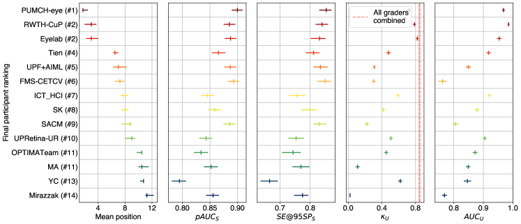
Figure 2: Final rankings of all participating teams. The teams are sorted by their final ranking and therefore also by their mean position. The mean position is shown in the left plot and the four challenge metrics are shown in the other four plots. The $\kappa_{U}$ of all human graders is indicated with a red dotted line. The width of the horizontal lines in all plots and the shaded area in the plot for $\kappa_{U}$ are 95% CIs. We consistently use the same colors to refer to teams in other figures in this manuscript.

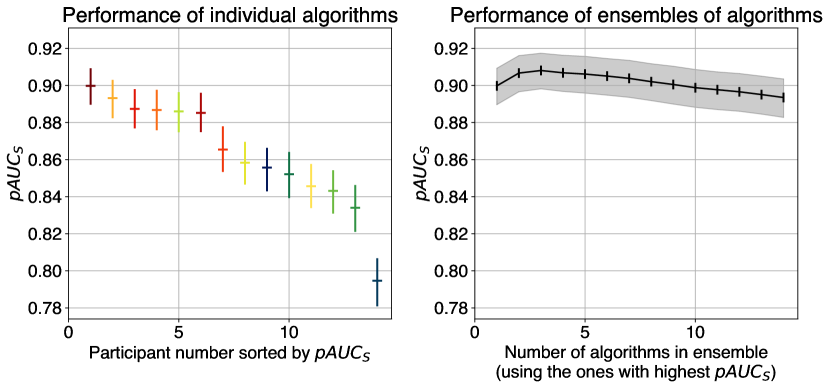
(a)

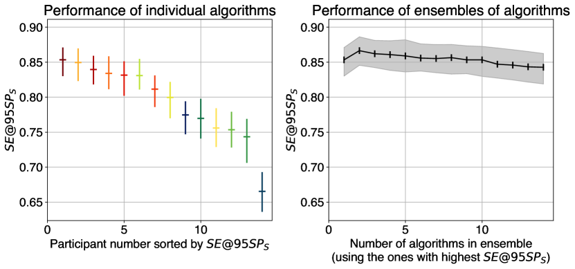
(b)

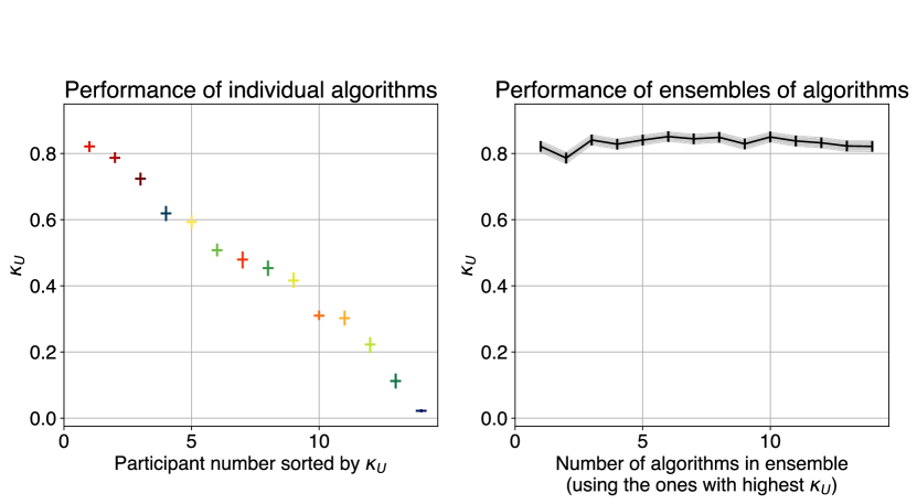
(c)

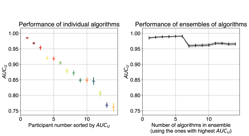
(d)

Figure 3: The four challenge metrics (3(a)) $pAUC_{S}$, (3(b)) $SE@95SP_{S}$, (3(c)) $\kappa_{U}$, and (3(d)) $AUC_{U}$ for the ensembles generated by incrementally fusing one algorithm at a time. The algorithms were fused by averaging the outputs of all algorithms in the ensemble. The vertical lines in the left plot and the shaded areas in the right plots indicate 95% CIs.

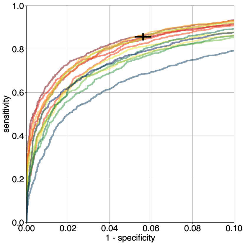
(a)

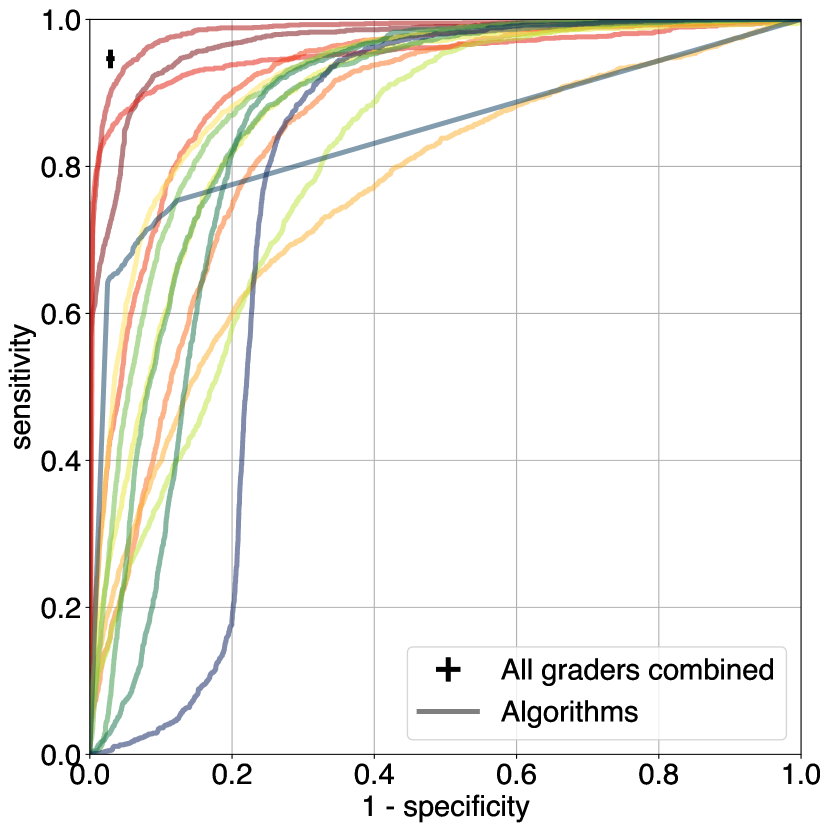
(b)

Figure 4: ROC curves for both challenge tasks. The sensitivity and specificity of all human graders on the AIROGS test set combined is indicated with black lines. Respectively, the width and height of the black horizontal and vertical line are 95% CIs. In (a), the partial ROC curve (90%-100% specificity) for screening is shown, with 1,602 positive (RG) and 8,134 negative (NRG) images from the AIROGS test set. In (b), the ROC curve for robustness is shown with 1,554 positive (ungradable) and 9,736 negative (gradable) images from the AIROGS test set.

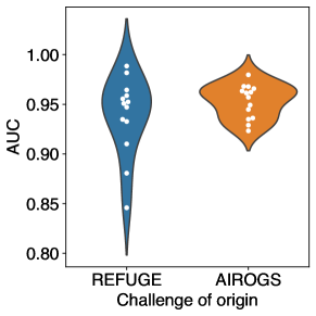
Figure 5: Comparison of the AIROGS and REFUGE algorithms, tested on the REFUGE test set, visualized as violin and swarm plots. The final algorithms that were developed for the REFUGE challenge itself and for the AIROGS challenge are shown on the left and right, respectively. The AIROGS algorithms were only trained on the AIROGS train set and were not retrained with the REFUGE dataset.

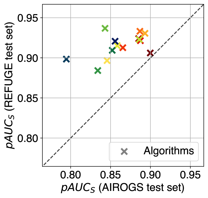
(a)

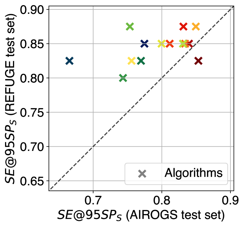
(b)

Figure 6: Performance of the participating AIROGS algorithms on the REFUGE dataset, compared to their performance on the AIROGS dataset. Both screening metrics (6(a)) $pAUC_{S}$ and (6(b)) $SE@95SP_{S}$ are shown.

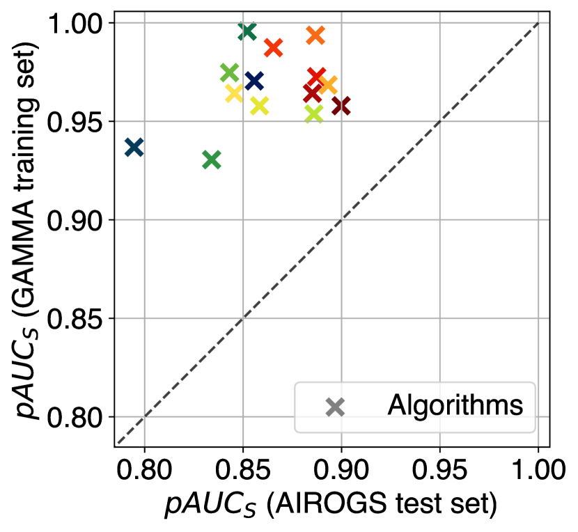
(a)

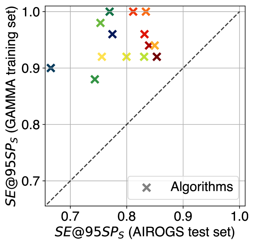
(b)

Figure 7: Performance of the participating AIROGS algorithms on the GAMMA dataset, compared to their performance on the AIROGS dataset. Both screening metrics (7(a)) $pAUC_{S}$ and (7(b)) $SE@95SP_{S}$ are shown.

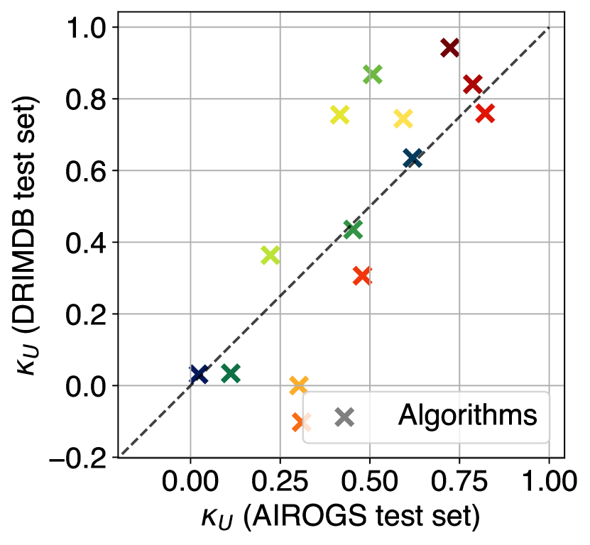
(a)

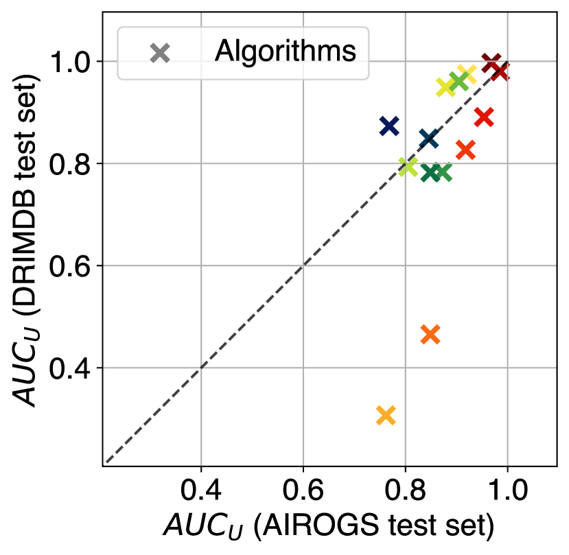
(b)

Figure 8: Performance of the participating AIROGS algorithms on the DRIMDB dataset, compared to their performance on the AIROGS dataset. Both robustness metrics (8(a)) $\kappa_{U}$ and (8(b)) $AUC_{U}$ are shown.

This section presents the glaucoma screening performance and robustness of the fourteen participating teams. The final rankings and mean positions of the teams are shown in the first plot of Fig. 2. Four teams shared a rank with another team, since their mean positions were exactly equal, causing there to be two teams for each of the ranks #2 and #11.

5.1 Glaucoma screening performance

The glaucoma screening performance of the participating teams is summarized in Fig. 2, showing $pAUC_{S}$ and $SE@95SP_{S}$ in the second and third plot, respectively. The highest scores for $pAUC_{S}$ and $SE@95SP_{S}$ were 0.90 (95% CI: 0.89 – 0.91) and 0.85 (95% CI: 0.83 – 0.87), respectively. These scores were both achieved by team PUMCH-eye.

Fig. 3(a) and Fig. 3(b) show the $pAUC_{S}$ and $SE@95SP_{S}$ for the ensembles when averaging the RG likelihood output $O_{1}$ of the best $M$ participants in terms of the relevant metric. An optimal $pAUC_{S}$ of 0.91 (95% CI: 0.90 – 0.92) was achieved at $M=3$. At $M=2$, an optimal value for $SE@95SP_{S}$ was reached, which was 0.87 (95% CI: 0.85 – 0.89).

Fig. 4(a) shows the partial ROC curves between 90% and 100% specificity for all participants. The plot also presents the sensitivity and specificity of the human graders with a 95% CI. These were 0.86 (95% CI: 0.84 – 0.87) and 0.94 (95% CI: 0.94 – 0.95), respectively.

In Fig. 5, we compare the performance on the REFUGE test set of the final AIROGS algorithms, which were trained on the AIROGS train set, to the performance of the algorithms that were submitted to the REFUGE challenge, which were trained on the REFUGE train set. The top three participants of the REFUGE algorithms achieved AUCs of 0.99, 0.98 and 0.96. For the AIROGS algorithms, the best three AUCs were 0.98, 0.97 and 0.97. The mean $\pm$ std. dev. AUC of all REFUGE and AIROGS algorithms were 0.94 $\pm$ 0.04 and 0.95 $\pm$ 0.02, respectively. Fig. 6 presents the relation between the two glaucoma screening performance metrics of all participating AIROGS algorithms on the AIROGS test set and that performance on the REFUGE test set. For both metrics, almost all AIROGS algorithms (except for team PUMCH-eye for $SE@95SP_{S}$) scored higher on REFUGE than on AIROGS. Of all AIROGS participants, the best $pAUC_{S}$ and $SE@95SP_{S}$ on REFUGE were 0.94 and 0.88, respectively.

In Fig. 7, the relation between the glaucoma performance of all participating AIROGS algorithms on the AIROGS test set and that performance on GAMMA is shown. For both screening metrics, all AIROGS algorithms scored higher on GAMMA than on AIROGS. Of all AIROGS participants, the best $pAUC_{S}$ and $SE@95SP_{S}$ on GAMMA were 1.0 and 1.0, respectively.

5.2 Robustness

The robustness metrics of the participating teams are summarized in Fig. 2, showing $\kappa_{U}$ and $AUC_{U}$ in the fourth and fifth plot, respectively. The highest scores for $\kappa_{U}$ and $AUC_{U}$ were 0.82 (95% CI: 0.80 – 0.84) and 0.99 (95% CI: 0.98 – 0.99), respectively. These scores were achieved by team Temirgali and RWTH-CuP, respectively.

Fig. 3(c) and Fig. 3(d) show the $\kappa_{U}$ and $AUC_{U}$ for the ensembles when averaging output $O_{3}$ and output $O_{4}$, respectively, of the $M$ best algorithms in terms of these respective metrics. An optimal $\kappa_{U}$ of 0.85 (95% CI: 0.84 – 0.86) was achieved at $M=6$. Also at $M=6$, an optimal value for $AUC_{U}$ was reached, which was 0.99 (95% CI: 0.99 – 0.99).

In Fig. 4(b), ROC curves for robustness are shown for all participants. The plot also presents the sensitivity and specificity for separating ungradable from gradable images of the human graders with a 95% CI. These were 0.95 (95% CI: 0.94 – 0.96) and 0.97 (95% CI: 0.97 – 0.97), respectively.

The results on the external DRIMDB dataset are shown in Fig. 8, indicating the relation between the ungradability metrics $\kappa_{U}$ and $AUC_{U}$ of all participating AIROGS algorithms on DRIMDB and those metrics on AIROGS. Of all AIROGS participants, the best $\kappa_{U}$ and $AUC_{U}$ on DRIMDB were 0.94 and 1.0, respectively.

6 Discussion

AI models have been shown to be effective at detecting glaucoma in CFPs, but most studies lack evidence of robustness to real-world scenarios in which unexpected OOD data can be presented due to various causes. To this end, we relied on the community to develop robust AI solutions for glaucoma screening based on the largest multi-center real-world CFP dataset with glaucoma labels. We organized the AIROGS challenge around this dataset, ensuring the resulting algorithms are reusable in a cloud-based environment. We applied these algorithms to ungradable data, while the participants could only train on gradable data to ensure robustness to any kind of ungradable data, and to other publicly available datasets to assess their generalization.

6.1 Overall findings

The team with the highest $SE@95SP_{S}$ scored expert-level screening performance on the AIROGS test set with a sensitivity of 0.85 (95% CI: 0.83 – 0.87) at 95% specificity, similar to the sensitivity of 0.86 (95% CI: 0.84 – 0.87) at a specificity of 0.94 (95% CI: 0.94 – 0.95) of human graders. The highest $pAUC_{S}$ that was achieved by any of the teams was 0.90 (95% CI: 0.89 – 0.91). Ensembling the different participating methods improved the screening performance even further, to 0.91 (95% CI: 0.90 – 0.92) and 0.87 (95% CI: 0.85 – 0.89) for $pAUC_{S}$ and $SE@95SP_{S}$, respectively. Seven out of fourteen teams exceeded the minimum performance of 80% sensitivity and 95% specificity that was required by human graders who were periodically monitored during the grading process. This shows these models can provide a similar performance to human graders for glaucoma screening, suggesting that AI can potentially play a role in an automated screening process.

We also evaluated the screening performance of the algorithms on two external test sets. Even though the algorithms were trained on AIROGS data, they achieved very high performances on the two external test sets, showing reproducible results in different sets and populations. On average, the participating AIROGS algorithms scored slightly higher on the REFUGE dataset than the REFUGE participants. We found that the participating algorithms scored substantially higher on these external datasets than on the AIROGS test set, indicating the value of a challenging real-world dataset. This strong generalization of the developed solutions also shows the potential of models trained on our dataset to be successfully implemented in screening programs with limited to no loss of performance.

The robustness to ungradable data in the AIROGS test set was evaluated for each team using the metrics $\kappa_{U}$ and $AUC_{U}$. The teams that performed the best in terms of these metrics achieved 0.82 (95% CI: 0.80 – 0.84) and 0.99 (95% CI: 0.98 – 0.99) for $\kappa_{U}$ and $AUC_{U}$, respectively. Human experts did reach a higher $\kappa_{U}$ of 0.85 (95% CI: 0.84-0.86) for this task. Moreover, they achieved a sensitivity of 0.95 (95% CI: 0.94 – 0.96) and a specificity of 0.97 (95% CI: 0.97 – 0.97) for detecting ungradable cases, while the team with the best $AUC_{U}$ achieved a lower sensitivity at 97% specificity of 0.90 (95% CI: 0.88-0.92). Although the teams achieved relatively high performances, they still achieved lower performance at the robustness task than human experts. This shows this task was especially challenging, possibly because the participating teams could not use ungradable development data or because their robustness approaches focused on specific forms of ungradability.

We also assessed robustness on the external DRIMDB dataset. The best scoring team on this dataset scored very high performances; they achieved 0.94 and 1.0 for $\kappa_{U}$ and $AUC_{U}$, respectively. These two metrics were lower on the AIROGS dataset for that team. This also indicates very strong generalization to other datasets for the robustness task. The high ungradability detection performance also indicates robustness to other diseases in the image, as diabetic retinopathy was prevalent in the gradable subset of DRIMDB and the best algorithms did not classify these diseases as ungradable.

A large difference in performance between participating teams can be observed, both for the screening and the robustness task. Therefore, we think it is important to identify which methodological choices were made predominantly by top performing teams. One of the most notable differences between the top three participants and the rest was the use of transformers. Outside of the top three, only the latest placed team used a transformer. Moreover, all best three participants manually labelled ODs for training either a segmentation or detection model to crop around the OD during pre-processing. Even though this was also done by two other teams, this seems like an effective strategy to achieve higher screening performance. A likely reason for the effectiveness of this approach is that most glaucoma-related imaging features can be found on or around the OD. This shows how a priori medical knowledge could still be of value even when large amount of data is available. A less important factor appears to be the number of manually labeled ODs. A possible reason for this could be that the OD detection or segmentation network is not required to be extremely accurate as combining a rough localization of the OD with a large enough padding margin could also suffice to crop the image during pre-processing.

Since the development set only consisted of images that were labeled gradable (either RG or NRG) and the use of external fundus data was prohibited, all teams came up with an uncertainty or OOD detection method based on the gradable data for the robustness task. The ungradability methods of the top three participants in terms of mean position, $\kappa_{U}$ and $AUC_{U}$, all revolved around the confidence of a neural network that localized the OD. Of the other participants, only the ninth placed team had such an approach. Apart from these methods based on OD detection, only team UPF+AIML implemented a different robustness technique that was also based on domain-knowledge. This raises the impression that solutions based on domain knowledge are more effective for robustness than more general OOD detection solutions. However, it still needs to be evaluated if such approaches are robust for other general tasks (not glaucoma screening) or other sources of OOD data.

For calculating the $\kappa_{U}$ metric, the participants were required to output a binary decision on ungradability. A popular approach, especially among the top participants, was to manually identify relatively low quality images in the development set and base a threshold for this binary output on that subset. This technique was employed by the best three, fifth, tenth and twelfth team in terms of $\kappa_{U}$. This indicates that this could be a successful approach, although not in general as the accuracy of this binary value is also highly dependent on the quality of the scalar output for ungradability $O_{4}$ that is being thresholded. We found the difference between the ranking in terms of $\kappa_{U}$ and $AUC_{U}$ of one team in particular stood out. Team YC ranked only eleventh for $AUC_{U}$ (which depended on the scalar output $O_{4}$), but ranked fourth in terms of $\kappa_{U}$ (which depended on the binary output $O_{3}$), indicating the approach they used for thresholding their scalar value was highly effective. The difference between their $AUC_{U}$ and $\kappa_{U}$ was 7, while the next biggest value of this difference was only 3. Team YC indeed came up with a relatively sophisticated method for binarizing $O_{4}$ compared to others, based on a Wilcoxon one-sample test to statistically test whether the mean of the predicted probabilties from a Monte-Carlo drop-out approach was 0.5 or not.

6.2 Strengths and limitations

The dataset presented in this paper substantially exceeds what was publicly available before in terms of number of images and patients. The dataset is also highly diverse because of the large number of different sites, cameras that were used and ethnicities. The quality of the labels was controlled by the initial and periodical evaluation of human graders, the fact that each image was independently labeled twice by two trained graders and, in case of disagreement, by a highly experienced reader. The participants submitted their solutions as containerized algorithms, allowing reproducibility, facilitating inference on other data, and preventing manual manipulation of the test set.

One of the rules of the AIROGS challenge was the prohibition of the use of external fundus data for development. A limitation of this work is the fact that we cannot be sure if any of the teams used such data in their development process. A possible approach to prevent this and making the process fairer is to have participants submit a containerized algorithm for training, which would be trained by the challenge organizers with private challenge training data. Nevertheless, with such an approach it would still be challenging and time-consuming for the challenge organizers to verify if the training containers do not contain any weights pre-trained on other data.

The dataset used for the challenge is diverse, but improvements could still be made in that respect. All screening sites were based across the United States of America, raising the question whether a more generalizable model could be obtained with data from across the world. On the other hand, we showed that many algorithms trained on the AIROGS dataset performed at least as well on three external test sets, of which two originated from China and one from Turkey, as on our internal test set.

Not all research groups working in the field of retinal image analysis participated in this challenge and many teams that joined the challenge did not submit a solution to the Final Test Phase. Possible reasons for this include that many teams saw their results did not match to ones already present on the leaderboard, that the barrier for some teams was too high to get a solution wrapped in a Docker container, or that they were not able to finish in time. Therefore we would like to stress the challenge is still open and we are curious to see if the community can make further improvements. After all, especially for the robustness task, there seems to be room for improvement, given the gap with the human grader performance.

6.3 Future directions

Based on the solutions that were presented by the teams, we think it would be valuable to combine methodologies from different participants and to work further on their ideas. For example, as we mentioned before, team YC apparently had a highly effective method for thresholding their ungradability scores as their $\kappa_{U}$ was very high compared to their $AUC_{U}$. A possible future direction would be to combine methods of high performance in terms of $AUC_{U}$ with the binarization technique from team YC. Moreover, we observed that algorithms which scored high in terms of robustness, used domain-knowledge for this aspect of the challenge. Possible future directions could be to explore other ways to incorporate domain-knowledge into an ungradability method. This observation also leads to the question whether there are more fields in medical image analysis in which domain-knowledge can be leveraged for uncertainty estimation and OOD detection.

Next to a decision on RG and NRG presence, the graders were asked to provide which clinical, glaucomatous features were present in the eyes they classified as RG, as listed in Section 2.1 and further described by [77]. This information was not yet included in the dataset release for this challenge, as it fell outside the scope of this challenge. Future solutions and challenges could be developed with this information, possibly resulting in more explainable algorithms.

This challenge only focused on classification based on a single CFP. It may be interesting to explore the effect on screening performance and robustness of including various types of metadata in our dataset, which we have available but have not been published yet. This metadata, although missing for some images, includes the camera type, age and anonymous patient identification (which can be used to link two eyes to a single patient).

7 Conclusions

We presented the results of community-acquired algorithms tested on real-world data for robust glaucoma screening from CFP. The best algorithms performed similarly in terms of screening to the carefully trained and selected human graders, and were shown to be effective at flagging images that could not be graded. Methodological choices predominantly made by the best teams included, for the screening task, the use of vision transformers and the incorporation of optic disc detection models in pre-processing and, for the robustness task, out-of-distribution detection approaches based on domain-knowledge. We hope the unprecedented size and real-world nature of the dataset we released and the algorithms that were developed using this dataset will help towards implementing robust AI for glaucoma screening.

References

- [1] Yih-Chung Tham, Xiang Li, Tien Y Wong, Harry A Quigley, Tin Aung, and Ching-Yu Cheng. Global prevalence of glaucoma and projections of glaucoma burden through 2040: a systematic review and meta-analysis. Ophthalmology, 121(11):2081–2090, 2014.
- [2] Palwasha Mokhles, Jan SAG Schouten, Henny JM Beckers, Augusto Azuara-Blanco, Anja Tuulonen, and Carroll AB Webers. A systematic review of end-of-life visual impairment in open-angle glaucoma: an epidemiological autopsy. Journal of Glaucoma, 25(7):623–628, 2016.
- [3] Paul JG Ernest, Michiel JWM Busch, Carroll AB Webers, Henny JM Beckers, Fred Hendrikse, Martin H Prins, and Jan SAG Schouten. Prevalence of end-of-life visual impairment in patients followed for glaucoma. Acta Ophthalmologica, 91(8):738–743, 2013.
- [4] Dorothea Peters, Boel Bengtsson, and Anders Heijl. Lifetime risk of blindness in open-angle glaucoma. American Journal of Ophthalmology, 156(4):724–730, 2013.
- [5] Robert N Weinreb, Tin Aung, and Felipe A Medeiros. The pathophysiology and treatment of glaucoma: a review. JAMA, 311(18):1901–1911, 2014.
- [6] Xiangyu Chen, Yanwu Xu, Fengshou Yin, Zhuo Zhang, Damon Wing Kee Wong, Tien Yin Wong, and Jiang Liu. Multiple ocular diseases detection based on joint sparse multi-task learning. In 2015 37th Annual International Conference of the IEEE Engineering in Medicine and Biology Society (EMBC), pages 5260–5263. IEEE, 2015.
- [7] Daniel Shu Wei Ting, Carol Yim-Lui Cheung, Gilbert Lim, Gavin Siew Wei Tan, Nguyen D Quang, Alfred Gan, Haslina Hamzah, Renata Garcia-Franco, Ian Yew San Yeo, Shu Yen Lee, et al. Development and validation of a deep learning system for diabetic retinopathy and related eye diseases using retinal images from multiethnic populations with diabetes. JAMA, 318(22):2211–2223, 2017.
- [8] Zhixi Li, Yifan He, Stuart Keel, Wei Meng, Robert T Chang, and Mingguang He. Efficacy of a deep learning system for detecting glaucomatous optic neuropathy based on color fundus photographs. Ophthalmology, 125(8):1199–1206, 2018.
- [9] Sonia Phene, R Carter Dunn, Naama Hammel, Yun Liu, Jonathan Krause, Naho Kitade, Mike Schaekermann, Rory Sayres, Derek J Wu, Ashish Bora, et al. Deep learning and glaucoma specialists: the relative importance of optic disc features to predict glaucoma referral in fundus photographs. Ophthalmology, 126(12):1627–1639, 2019.
- [10] Thomas W Rogers, Nicolas Jaccard, Francis Carbonaro, Hans G Lemij, Koenraad A Vermeer, Nicolaas J Reus, and Sameer Trikha. Evaluation of an ai system for the automated detection of glaucoma from stereoscopic optic disc photographs: the european optic disc assessment study. Eye, 33(11):1791–1797, 2019.
- [11] Emma Beede, Elizabeth Baylor, Fred Hersch, Anna Iurchenko, Lauren Wilcox, Paisan Ruamviboonsuk, and Laura M Vardoulakis. A human-centered evaluation of a deep learning system deployed in clinics for the detection of diabetic retinopathy. In Proceedings of the 2020 CHI Conference on Human Factors in Computing Systems, pages 1–12, 2020.
- [12] Zhuo Zhang, Feng Shou Yin, Jiang Liu, Wing Kee Wong, Ngan Meng Tan, Beng Hai Lee, Jun Cheng, and Tien Yin Wong. Origa-light: An online retinal fundus image database for glaucoma analysis and research. In 2010 Annual International Conference of the IEEE Engineering in Medicine and Biology, pages 3065–3068. IEEE, 2010.
- [13] Francisco Fumero, Silvia Alayón, José L Sanchez, Jose Sigut, and M Gonzalez-Hernandez. Rim-one: An open retinal image database for optic nerve evaluation. In 24th International Symposium on Computer-Based Medical Systems (CBMS), pages 1–6. IEEE, 2011.
- [14] Jan Odstrcilik, Radim Kolar, Attila Budai, Joachim Hornegger, Jiri Jan, Jiri Gazarek, Tomas Kubena, Pavel Cernosek, Ondrej Svoboda, and Elli Angelopoulou. Retinal vessel segmentation by improved matched filtering: evaluation on a new high-resolution fundus image database. IET Image Processing, 7(4):373–383, 2013.
- [15] Jayanthi Sivaswamy, S Krishnadas, Arunava Chakravarty, G Joshi, A Syed Tabish, et al. A comprehensive retinal image dataset for the assessment of glaucoma from the optic nerve head analysis. JSM Biomedical Imaging Data Papers, 2(1):1004, 2015.
- [16] Sven Holm, Greg Russell, Vincent Nourrit, and Niall McLoughlin. Dr hagis—a fundus image database for the automatic extraction of retinal surface vessels from diabetic patients. Journal of Medical Imaging, 4(1):014503, 2017.
- [17] José Ignacio Orlando, João Barbosa Breda, Karel van Keer, Matthew B Blaschko, Pablo J Blanco, and Carlos A Bulant. Towards a glaucoma risk index based on simulated hemodynamics from fundus images. In International Conference on Medical Image Computing and Computer-Assisted Intervention, pages 65–73. Springer, 2018.
- [18] José Ignacio Orlando, Huazhu Fu, João Barbosa Breda, Karel van Keer, Deepti R Bathula, Andrés Diaz-Pinto, Ruogu Fang, Pheng-Ann Heng, Jeyoung Kim, JoonHo Lee, et al. REFUGE challenge: A unified framework for evaluating automated methods for glaucoma assessment from fundus photographs. Medical image analysis, 59:101570, 2020.
- [19] Huihui Fang, Fei Li, Huazhu Fu, Xu Sun, Xingxing Cao, Jaemin Son, Shuang Yu, Menglu Zhang, Chenglang Yuan, Cheng Bian, et al. Refuge2 challenge: Treasure for multi-domain learning in glaucoma assessment. arXiv preprint arXiv:2202.08994, 2022.
- [20] Junde Wu, Huihui Fang, Fei Li, Huazhu Fu, Fengbin Lin, Jiongcheng Li, Lexing Huang, Qinji Yu, Sifan Song, Xingxing Xu, et al. Gamma challenge: glaucoma grading from multi-modality images. arXiv preprint arXiv:2202.06511, 2022.
- [21] Jorge Cuadros and George Bresnick. Eyepacs: an adaptable telemedicine system for diabetic retinopathy screening. Journal of diabetes science and technology, 3(3):509–516, 2009.
- [22] Nicolaas J Reus, Hans G Lemij, David F Garway-Heath, P Juhani Airaksinen, Alfonso Anton, Alain M Bron, Christoph Faschinger, Gábor Holló, Michele Iester, Jost B Jonas, et al. Clinical assessment of stereoscopic optic disc photographs for glaucoma: the european optic disc assessment trial. Ophthalmology, 117(4):717–723, 2010.
- [23] Ugur Sevik, Cemal Kose, Tolga Berber, and Hidayet Erdol. Identification of suitable fundus images using automated quality assessment methods. Journal of biomedical optics, 19(4):046006, 2014.
- [24] Donna Katzman McClish. Analyzing a portion of the roc curve. Medical decision making, 9(3):190–195, 1989.
- [25] Hanna Vaahtoranta-Lehtonen, Anja Tuulonen, Pasi Aronen, Harri Sintonen, Liisa Suoranta, Niina Kovanen, Miika Linna, Esa Läärä, and Antti Malmivaara. Cost effectiveness and cost utility of an organized screening programme for glaucoma. Acta Ophthalmologica Scandinavica, 85(5):508–518, 2007.
- [26] Margriet M de Vries, Remco Stoutenbeek, Rogier PHM Müskens, and Nomdo M Jansonius. Glaucoma screening during regular optician visits: the feasibility and specificity of screening in real life. Acta ophthalmologica, 90(2):115–121, 2012.
- [27] Carolyn M Rutter. Bootstrap estimation of diagnostic accuracy with patient-clustered data. Academic radiology, 7(6):413–419, 2000.
- [28] Diederik P Kingma and Jimmy Ba. Adam: A method for stochastic optimization. arXiv preprint arXiv:1412.6980, 2014.
- [29] Ilya Loshchilov and Frank Hutter. Decoupled weight decay regularization. arXiv preprint arXiv:1711.05101, 2017.
- [30] Pierre Foret, Ariel Kleiner, Hossein Mobahi, and Behnam Neyshabur. Sharpness-aware minimization for efficiently improving generalization. arXiv preprint arXiv:2010.01412, 2020.
- [31] Kaiming He, Xinlei Chen, Saining Xie, Yanghao Li, Piotr Dollár, and Ross Girshick. Masked autoencoders are scalable vision learners. In Proceedings of the IEEE/CVF Conference on Computer Vision and Pattern Recognition, pages 16000–16009, 2022.
- [32] Qizhe Xie, Minh-Thang Luong, Eduard Hovy, and Quoc V Le. Self-training with noisy student improves imagenet classification. In Proceedings of the IEEE/CVF conference on computer vision and pattern recognition, pages 10687–10698, 2020.
- [33] Ekin D Cubuk, Barret Zoph, Dandelion Mane, Vijay Vasudevan, and Quoc V Le. Autoaugment: Learning augmentation policies from data. arXiv preprint arXiv:1805.09501, 2018.
- [34] Ekin D Cubuk, Barret Zoph, Jonathon Shlens, and Quoc V Le. Randaugment: Practical automated data augmentation with a reduced search space. In Proceedings of the IEEE/CVF conference on computer vision and pattern recognition workshops, pages 702–703, 2020.
- [35] Samuel G Müller and Frank Hutter. Trivialaugment: Tuning-free yet state-of-the-art data augmentation. In Proceedings of the IEEE/CVF International Conference on Computer Vision, pages 774–782, 2021.
- [36] He Wang, Hongyi Sun, Yi Fang, Shuo Li, Ming Feng, and Renzhi Wang. A workflow for computer-aided diagnosis of glaucoma. In 2022 IEEE International Symposium on Biomedical Imaging Challenges (ISBIC), pages 1–4. IEEE, 2022.
- [37] Firas Khader, Christoph Haarburger, Jörg-Christian Kirr, Marcel Menke, Jakob Nikolas Kather, Johannes Stegmaier, Christiane Kuhl, Sven Nebelung, and Daniel Truhn. Elevating fundoscopic evaluation to expert level-automatic glaucoma detection using data from the airogs challenge. In 2022 IEEE International Symposium on Biomedical Imaging Challenges (ISBIC), pages 1–4. IEEE, 2022.
- [38] Teresa Araújo, Guilherme Aresta, and Hrvoje Bogunović. Deep dirichlet uncertainty for unsupervised out-of-distribution detection of eye fundus photographs in glaucoma screening. In 2022 IEEE International Symposium on Biomedical Imaging Challenges (ISBIC), pages 1–5. IEEE, 2022.
- [39] Tete Xiao, Yingcheng Liu, Bolei Zhou, Yuning Jiang, and Jian Sun. Unified perceptual parsing for scene understanding. In Proceedings of the European conference on computer vision (ECCV), pages 418–434, 2018.
- [40] Gilad Sharir, Asaf Noy, and Lihi Zelnik-Manor. An image is worth 16x16 words, what is a video worth? arXiv preprint arXiv:2103.13915, 2021.
- [41] Ze Liu, Yutong Lin, Yue Cao, Han Hu, Yixuan Wei, Zheng Zhang, Stephen Lin, and Baining Guo. Swin transformer: Hierarchical vision transformer using shifted windows. In Proceedings of the IEEE/CVF International Conference on Computer Vision, pages 10012–10022, 2021.
- [42] Hugo Touvron, Matthieu Cord, Matthijs Douze, Francisco Massa, Alexandre Sablayrolles, and Hervé Jégou. Training data-efficient image transformers & distillation through attention. In International Conference on Machine Learning, pages 10347–10357. PMLR, 2021.
- [43] Mingxing Tan and Quoc Le. Efficientnet: Rethinking model scaling for convolutional neural networks. In International conference on machine learning, pages 6105–6114. PMLR, 2019.
- [44] Mingxing Tan and Quoc Le. Efficientnetv2: Smaller models and faster training. In International conference on machine learning, pages 10096–10106. PMLR, 2021.
- [45] Glenn Jocher, Alex Stoken, Jirka Borovec, Liu Changyu, Adam Hogan, L Diaconu, F Ingham, J Poznanski, J Fang, L Yu, et al. ultralytics/yolov5. Zenodo, 2020.
- [46] Temirgali Aimyshev and Kanat Eleusiz. Glaucoma detection algorithm for the artificial intelligence for robust glaucoma screening challenge, 2022.
- [47] Alexey Dosovitskiy, Lucas Beyer, Alexander Kolesnikov, Dirk Weissenborn, Xiaohua Zhai, Thomas Unterthiner, Mostafa Dehghani, Matthias Minderer, Georg Heigold, Sylvain Gelly, et al. An image is worth 16x16 words: Transformers for image recognition at scale. arXiv preprint arXiv:2010.11929, 2020.
- [48] Tien-Dung Le. Combination of supervised learning and unsupervised learning to detect ungradable images in the airogs challenge, 2022.
- [49] Gao Huang, Zhuang Liu, Laurens Van Der Maaten, and Kilian Q Weinberger. Densely connected convolutional networks. In Proceedings of the IEEE conference on computer vision and pattern recognition, pages 4700–4708, 2017.
- [50] Adrian Galdran, Gustavo Carneiro, and Miguel A. Gonzlez Ballester. Open-set glaucoma screening from eye fundus images: Domain knowledge to the rescue, 2022.
- [51] Andrew G Howard, Menglong Zhu, Bo Chen, Dmitry Kalenichenko, Weijun Wang, Tobias Weyand, Marco Andreetto, and Hartwig Adam. Mobilenets: Efficient convolutional neural networks for mobile vision applications. arXiv preprint arXiv:1704.04861, 2017.
- [52] Densen Puthussery, P S Hrishikesh, R G Devika, and C V Jiji. A self-supervised approach for glaucoma screening, 2022.
- [53] Tsung-Yi Lin, Priya Goyal, Ross Girshick, Kaiming He, and Piotr Dollár. Focal loss for dense object detection. In Proceedings of the IEEE international conference on computer vision, pages 2980–2988, 2017.
- [54] Poojan Oza and Vishal M Patel. One-class convolutional neural network. IEEE Signal Processing Letters, 26(2):277–281, 2018.
- [55] Zekang Yang, Hong Liu, and Zihao Shang. Deep learning for referable glaucoma screening and out-of-distribution detection, 2022.
- [56] Satoshi Kondo, Satoshi Kasai, and Kosuke Hirasawa. Computer aided diagnosis and out-of-distribution detection in glaucoma screening using color fundus photography. arXiv preprint arXiv:2202.11944, 2022.
- [57] Irwan Bello, William Fedus, Xianzhi Du, Ekin Dogus Cubuk, Aravind Srinivas, Tsung-Yi Lin, Jonathon Shlens, and Barret Zoph. Revisiting resnets: Improved training and scaling strategies. Advances in Neural Information Processing Systems, 34:22614–22627, 2021.
- [58] Weitang Liu, Xiaoyun Wang, John Owens, and Yixuan Li. Energy-based out-of-distribution detection. Advances in Neural Information Processing Systems, 33:21464–21475, 2020.
- [59] Yiyou Sun, Chuan Guo, and Yixuan Li. React: Out-of-distribution detection with rectified activations. Advances in Neural Information Processing Systems, 34:144–157, 2021.
- [60] Edward Wang, Ashritha Durvasula, Daisy Deng, Asaanth Sivajohan, Edward Ho, and Kevin Lane. Ensemble network for glaucoma screening in airogs challenge, 2022.
- [61] Jie Hu, Li Shen, and Gang Sun. Squeeze-and-excitation networks. In Proceedings of the IEEE Conference on Computer Vision and Pattern Recognition, pages 7132–7141, 2018.
- [62] Karen Simonyan and Andrew Zisserman. Very deep convolutional networks for large-scale image recognition. arXiv preprint arXiv:1409.1556, 2014.
- [63] Christian Szegedy, Vincent Vanhoucke, Sergey Ioffe, Jon Shlens, and Zbigniew Wojna. Rethinking the inception architecture for computer vision. In Proceedings of the IEEE conference on computer vision and pattern recognition, pages 2818–2826, 2016.
- [64] Diederik P Kingma and Max Welling. Auto-encoding variational bayes. arXiv preprint arXiv:1312.6114, 2013.
- [65] Jónathan Heras, Didac Royo, and Miguel Ángel Zapata. A good closed-set classifier is all you need for the airogs challenge, 2022.
- [66] Sagar Vaze, Kai Han, Andrea Vedaldi, and Andrew Zisserman. Open-set recognition: A good closed-set classifier is all you need. arXiv preprint arXiv:2110.06207, 2021.
- [67] Arthur P Dempster. A generalization of bayesian inference. Journal of the Royal Statistical Society: Series B (Methodological), 30(2):205–232, 1968.
- [68] Ramprasaath R Selvaraju, Michael Cogswell, Abhishek Das, Ramakrishna Vedantam, Devi Parikh, and Dhruv Batra. Grad-cam: Visual explanations from deep networks via gradient-based localization. In Proceedings of the IEEE International Conference on Computer Vision, pages 618–626, 2017.
- [69] Mustafa Arikan. Multi-model ensemble for robust glaucoma screening, 2022.
- [70] Christian Szegedy, Sergey Ioffe, Vincent Vanhoucke, and Alexander A Alemi. Inception-v4, Inception-ResNet and the impact of residual connections on learning. In Thirty-first AAAI Conference on Artificial Intelligence, 2017.
- [71] Yeong Chan Lee, Hyun Bin Cho, and Yoon Ho Choi. Classification for referable glaucoma with fundus photographs using multimodal deep learning, 2022.
- [72] Olaf Ronneberger, Philipp Fischer, and Thomas Brox. U-Net: Convolutional networks for biomedical image segmentation. In International Conference on Medical image computing and computer-assisted intervention, pages 234–241. Springer, 2015.
- [73] Yarin Gal and Zoubin Ghahramani. Dropout as a bayesian approximation: Representing model uncertainty in deep learning. In international conference on machine learning, pages 1050–1059. PMLR, 2016.
- [74] Abdul Qayyum, Moona Mazher, and Imran Razzak. Convnexts and vision transformer based framework for glaucoma screening, 2022.
- [75] Zhuang Liu, Hanzi Mao, Chao-Yuan Wu, Christoph Feichtenhofer, Trevor Darrell, and Saining Xie. A convnet for the 2020s. In Proceedings of the IEEE/CVF Conference on Computer Vision and Pattern Recognition, pages 11976–11986, 2022.
- [76] Koby Bibas, Meir Feder, and Tal Hassner. Single layer predictive normalized maximum likelihood for out-of-distribution detection. Advances in Neural Information Processing Systems, 34:1179–1191, 2021.
- [77] Hans G Lemij, Coen de Vente, Clara Sánchez, Jorge Cuadros, Nicolas Jaccard, and Koen Vermeer. Glaucomatous features in fundus photographs of eyes with ’referable glaucoma’ of a large population based labeled data set for training an artificial intelligence (AI) algorithm for glaucoma screening. In Association for Research in Vision and Ophthalmology, volume 63, pages 2041–A0482. The Association for Research in Vision and Ophthalmology, 2022.