All-coupling solution for the continuous polaron problem in the Schrödinger representation

Abstract

The solution for the large-radius Fröhlich polaron in the Schrödinger representation of the quantum theory is constructed in the entire range of variation of the coupling constant. The energy and the effective mass of the polaron are calculated by simple algebraic transformations and are analogous to the results found by Feynman on the basis of the variational principle for the path-integrals of this system. It allows us to solve the long-lived problem of the inequalities of the functional and operator approaches for the polaron problem. The developed method is important for other models of particle-field interaction including those ones for which the standard perturbation theory is divergent.

I Introduction

Presently it is well known that the polaron problem has broader significance than simply a model of the interaction between an electron and phonons in the ionic crystal as it was introduced by Fröhlich Fröhlich (1954). It is important for description of charge carriers in inorganic and organic matter interacting with ion vibrations Li et al. (2019); Yakaboylu and Lemeshko (2018). The corresponding electron-phonon interaction causes phase transitions, including superconductivity and dominates the transport properties of many metals and semiconductors (see for example, book Alexandrov and Devreese (2010) and review Devreese and Alexandrov (2009) and citations therein).

Hamiltonian of the polaron problem is also important as a fundamental model of the interaction between a particle and a quantum field. In this problem various nonperturbative methods of quantum field theory can be verified for the entire range of variation of the coupling constant $\alpha$ of the interaction between an electron and a quantum field Mitra et al. (1987). Like any other quantum system the polaron can be described both in the framework of the solution of the Schrödinger equation and by using the Feynman path-integral formalism Feynman (1955a). The former approach allowed one to introduce the idea of a self-localized polaron Pekar (1963) and to find the exact asymptotic value for the ground state energy $E(\alpha)$ of the system in the strong coupling limit $\alpha\gg 1$ Bogoliubov (1950). While the latter approach provided a uniform approximation for the energy of the system in the whole range of the variation of the coupling constant Feynman (1955b). It is important to notice that the solution for the strong coupling ($\alpha\gg 1$) is fundamentally different from the solution in the case of weak coupling $\alpha\ll 1$ when the standard perturbation theory can be applied Mitra et al. (1987).

The great advantage of Feynman variational principle for the path integrals is the possibility to calculate the polaron binding energy $E(\alpha)$ as the continuous function for any $\alpha$. In addition it allows one to find the lowest estimation for the polaron binding energy in the intermediate coupling regime by the functional integrals numerically. The effective diagrammatic quantum Monte Carlo algorithm was developed for the Fröhlich polaron in the path integral representation Mishchenko and Nagaosa (2007); Mishchenko et al. (2000); Hahn et al. (2018). It was considered as an important argument for the advantage of the functional approach in the quantum field theory in comparison with the Schrödinger representation.

There were a lot of attempts Tokuda (1982); de Bodas and Hipólito (1983); Feranchuk et al. (1984); Das Sarma (1985); Lepine (1985) to calculate the ground state energy with the help of variational principle for the Schrödinger representation of the polaron problem for all values of the coupling constant $\alpha$ (all-coupling polaron). However, a particular choice of the trial functions led to the singularity for the energy of the system $E(\alpha)$ near the point $\alpha\simeq 7$. These results caused the discussion about existence of the “phase transition” between two qualitatively different states of the polaron (see review Gerlach and Löwen (1991) on this problem). In a series of papers cited in Gerlach and Löwen (1991) it was proven that the function $E(\alpha)$ is analytical for any value of $\alpha$ and the “phase transition” does not exist. Strict mathematical investigation of the polaron problem in the strong coupling limit was recently considered in the work Lieb and Seiringer (2020). However, it is important to stress that till now no constructive computational algorithm or trial wave function for variational approach are developed for all-coupling solution of the polaron problem in the Schrödinger representation. The construction of such algorithm is of great interest not only for the polaron problem but also for non-perturbative description and analysis of the renormalization for other models in the quantum field theory Feranchuk et al. (2015).

In the present paper we use operator method (OM) for calculation of the ground state energy of the polaron problem for all values of the coupling constant $\alpha$ in the Schrödinger representation. The OM was introduced in the paper Feranchuk and Komarov (1982a); Feranchuk et al. (1995) and was effectively used later on for many quantum systems Feranchuk et al. (2015); Skoromnik and Feranchuk (2017). It leads to the fast convergent series for the solutions of the Schrödinger equation. This method was also applied for regular perturbation series in the polaron problem Feranchuk and Komarov (1982b) but it was considered only in the strong coupling limit.

In our work we for the first time demonstrate that in the case of Fröhlich Hamiltonian the two first terms of the OM series over $\alpha$ lead to the function $E(\alpha)$ and the effective mass $m_{p}(\alpha)$ of the polaron which fairly well coincide with Feynman’s results. These functions can be calculated by rather simple analytical expressions and lead to the correct asymptotic limits $\alpha\ll 1$ and $\alpha\gg 1$. In addition, good accuracy is achieved for intermediate coupling with less numerical efforts as in comparison with the path integral formalism. It seems to us that the results make more clear and descriptive the question about the ground state of the polaron and confirm the equivalence of the path integral and operator approaches for description of quantum systems. Our analysis is important for application of the self-localized states for other models of the particle-field interactions even in the case when conventional perturbation theory includes both the infrared and ultraviolet divergences Skoromnik et al. (2015).

II Zeroth order approximation for the ground state energy

Let us examine the Fröhlich Hamiltonian for the system consisting of a nonrelativistic electron that interacts with a quantum field of optical phonons

$$\hat{H} =\frac{\hat{\bm{p}}^{2}}{2}+2^{5/4}\sqrt{\frac{\pi\alpha}{\Omega}}\sum_{\bm{k}}\frac{\hat{q}_{\bm{k}}}{k}e^{\mathrm{i}\bm{k}\cdot\bm{r}}+\sum_{\bm{k}}\hat{c}^{\dagger}_{\bm{k}}\hat{c}_{\bm{k}}.$$ (1)

Here the natural units with $\hbar=c=m=1$ are chosen; $\hat{c}^{\dagger}_{\bm{k}}$ and $\hat{c}_{\bm{k}}$ are the phonon creation and annihilation operators and $\hat{q}_{\bm{k}}$ is the coordinate operator of the phonon field

$$\hat{q}_{\bm{k}}=\frac{1}{\sqrt{2}}(\hat{c}_{\bm{k}}+\hat{c}^{{\dagger}}_{-\bm{k}}).$$

Let us also represent the electron coordinate $\hat{\bm{r}}$ and momentum $\hat{\bm{p}}$ through the creation and annihilation operators, which allow us later to perform all calculations in the algebraic form without solutions of differential equations:

$$\hat{x}_{\lambda}=\frac{\hat{a}_{\lambda}+\hat{a}^{{\dagger}}_{\lambda}}{\sqrt{2\omega}},\ \hat{p}_{\lambda}=i\sqrt{\omega}\frac{\hat{a}^{{\dagger}}_{\lambda}-\hat{a}_{\lambda}}{\sqrt{2}},\ [\hat{a}_{\lambda},\hat{a}_{\mu}^{{\dagger}}]=\delta_{\lambda\mu},$$ (2)

with a free parameter $\omega$. $\lambda$, $\mu$ numerate three degrees of freedom of the particle. Recently it was also shown that the polaron can be described in an algebraic form by $q$-deformed Lie algebra Yakaboylu (2022).

As it was firstly shown by Ref. Pekar (1963), the electron-phonon interaction leads to the formation of the self-localized state of the electron in the potential field of the phonons. In order to take into account this effect we apply the canonical transformation of the field operators

$$\hat{q}_{\bm{k}}=u_{\bm{k}}+\hat{Q}_{\bm{k}};\ \hat{c}_{\bm{k}}=\frac{u_{\bm{k}}}{\sqrt{2}}+\hat{b}_{\bm{k}},$$ (3)

with the classical component of the field $u_{\bm{k}}$ , which will be defined later.

The main idea of the OM is based on including in the zeroth-order Hamiltonian $\hat{H}_{0}$ the terms from the full Hamiltonian that commute with the operators of the number of the excitations

$$\hat{n}_{\lambda} =\hat{a}^{{\dagger}}_{\lambda}\hat{a}_{\lambda},$$ (4)

$$\hat{N}_{\bm{k}} =\hat{b}^{{\dagger}}_{\bm{k}}\hat{b}_{\bm{k}}.$$ (5)

We now express $\hat{H}$ in terms of new operators. For this purpose we use the operator identity

$$\exp\left[\frac{ik_{\lambda}(\hat{a}_{\lambda}+\hat{a}^{{\dagger}}_{\lambda})}{\sqrt{2\omega}}\right]=e^{-\frac{k^{2}}{4\omega}}\exp\left(\frac{ik_{\lambda}\hat{a}^{{\dagger}}_{\lambda}}{\sqrt{2\omega}}\right)\exp\left(\frac{ik_{\lambda}\hat{a}_{\lambda}}{\sqrt{2\omega}}\right),$$ (6)

and split the Hamiltonian (1) into two parts

$$\hat{H}=\hat{H}_{0}+\hat{H}_{1},$$

where

$$\hat{H}_{0} =\frac{3}{4}\omega+\frac{\omega}{2}(2\hat{a}^{{\dagger}}_{\lambda}\hat{a}_{\lambda}-\hat{a}^{{\dagger}}_{\lambda}\hat{a}^{{\dagger}}_{\lambda}-\hat{a}_{\lambda}\hat{a}_{\lambda})$$

$$+\frac{1}{2}\sum_{\bm{k}}\left[u_{\bm{k}}u_{-\bm{k}}+\frac{1}{\sqrt{2}}(u_{\bm{k}}\hat{b}^{{\dagger}}_{\bm{k}}+u^{*}_{\bm{k}}\hat{b}_{\bm{k}})+\hat{b}^{{\dagger}}_{\bm{k}}\hat{b}_{\bm{k}}\right]$$ (7)

$$+\xi\sum_{\bm{k}}\frac{e^{-\frac{k^{2}}{4\omega}}}{k}\left[\hat{Q}_{\bm{k}}+u_{\bm{k}}\left(1-\frac{k_{\lambda}k_{\mu}}{4\omega}(2\hat{a}^{{\dagger}}_{\lambda}\hat{a}_{\mu}+\hat{a}^{{\dagger}}_{\lambda}\hat{a}^{{\dagger}}_{\mu}+\hat{a}_{\lambda}\hat{a}_{\mu})\right)\right],$$

and

$$\hat{H}_{1} =\xi\sum_{\bm{k}}\frac{e^{-\frac{k^{2}}{4\omega}}}{k}\Bigg{[}(\hat{Q}_{\bm{k}}+u_{\bm{k}})\left(\exp\left(\frac{ik_{\lambda}\hat{a}^{{\dagger}}_{\lambda}}{\sqrt{2\omega}}\right)\exp\left(\frac{ik_{\lambda}\hat{a}_{\lambda}}{\sqrt{2\omega}}\right)-1\right)$$

$$+u_{\bm{k}}\frac{k_{\lambda}k_{\mu}}{4\omega}(2\hat{a}^{{\dagger}}_{\lambda}\hat{a}_{\mu}+\hat{a}^{{\dagger}}_{\lambda}\hat{a}^{{\dagger}}_{\mu}+\hat{a}_{\lambda}\hat{a}_{\mu})\Bigg{]},$$ (8)

with

$$\hat{Q}_{\bm{k}}=\frac{\hat{b}^{{\dagger}}_{-\bm{k}}+\hat{b}_{\bm{k}}}{\sqrt{2}};\quad\xi=2^{5/4}\sqrt{\frac{\pi\alpha}{\Omega}}.$$

The operator (7) is reduced to the diagonal form if we choose the following values for the parameters $u_{k}$ and $\omega$

$$\omega =\frac{4\alpha^{2}}{9\pi};$$ (9)

$$u_{k} =-2^{5/4}\sqrt{\frac{\pi\alpha}{\Omega}}\frac{e^{-\frac{k^{2}}{4\omega}}}{k};$$ (10)

and looks

$$\hat{H}_{0}=-\frac{\alpha^{2}}{3\pi}+\frac{4\alpha^{2}}{9\pi}\hat{a}^{{\dagger}}_{\lambda}\hat{a}_{\lambda}+\sum_{\bm{k}}\hat{b}^{{\dagger}}_{\bm{k}}\hat{b}_{\bm{k}}.$$ (11)

Consequently the polaron ground state vector and energy in the zeroth approximation are defined as follows

$$E_{0}^{(0)} =-\frac{\alpha^{2}}{3\pi}$$ (12)

$$\hat{a}_{\lambda}|\psi_{0}\rangle =\hat{b}_{\bm{k}}|\psi_{0}\rangle=0.$$ (13)

The zeroth-order approximation alone does not provide the correct asymptotic behavior for the energy of the system for the case of weak coupling ($E\sim\alpha$). Therefore, we should take into account the second-order correction, where we expect the restoration of the correct asymptotic. We also notice here that this is a peculiar property of the operator method where the second-order correction restores the correct asymptotic behavior Feranchuk et al. (2015).

III Second order approximation for the ground state energy

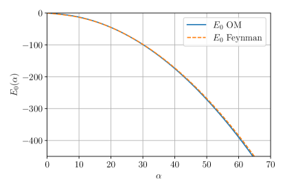
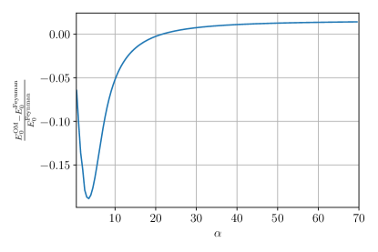
Figure 1: The polaron ground state energy and the relative difference as a function of $\alpha$ calculated by Feynman and our analytical formula

Let us consider the perturbation series on the operator $\hat{H}_{1}$ for the ground state energy. The first-order correction is equal to zero identically and the second-order one is defined by the formula

$$E_{0}^{(2)}=-\langle\psi_{0}|\hat{H}_{1}[E_{0}^{(0)}-\hat{H}_{0}]^{-1}\hat{H}_{1}|\psi_{0}\rangle.$$ (14)

It is evident that the ground state should be excluded from the resolvent spectrum. The calculation of (14) may be fulfilled in the operator form if we use the integral representation

$$E_{0}^{(2)}=\int_{0}^{\infty}dx\langle\psi_{0}|\hat{H}_{1}e^{-(\omega\hat{n}+\sum_{\bm{k}}\hat{N}_{\bm{k}})x}\hat{H}_{1}|\psi_{0}\rangle.$$ (15)

Let us calculate this value with the operator (8) represented in the normal form

$$\hat{H}_{1}|\psi_{0}\rangle=\xi\sum_{\bm{k}}\frac{e^{-\frac{k^{2}}{4\omega}}}{k}\Bigg{[}\left(\frac{\hat{b}^{{\dagger}}_{-\bm{k}}}{\sqrt{2}}+u_{\bm{k}}\right)\left(\exp\left(\frac{ik_{\lambda}\hat{a}^{{\dagger}}_{\lambda}}{\sqrt{2\omega}}\right)-1\right)$$

$$+u_{\bm{k}}\frac{k_{\lambda}k_{\mu}}{4\omega}\hat{a}^{{\dagger}}_{\lambda}\hat{a}^{{\dagger}}_{\mu}\Bigg{]}|\psi_{0}\rangle,$$ (16)

$$[e^{-(\omega\hat{n}+\sum_{\bm{k}}\hat{N}_{\bm{k}})x}]\hat{H}_{1}|\psi_{0}\rangle=\xi\sum_{\bm{k}}\frac{e^{-\frac{k^{2}}{4\omega}}}{k}\Bigg{[}\left(\frac{\hat{b}^{{\dagger}}_{-\bm{k}}e^{-x}}{\sqrt{2}}+u_{\bm{k}}\right)\left(\exp\left(\frac{ik_{\lambda}\hat{a}^{{\dagger}}_{\lambda}e^{-\omega x}}{\sqrt{2\omega}}\right)-1\right)+u_{\bm{k}}\frac{k_{\lambda}k_{\mu}}{4\omega}\hat{a}^{{\dagger}}_{\lambda}\hat{a}^{{\dagger}}_{\mu}e^{-2\omega x}\Bigg{]}|\psi_{0}\rangle,$$ (17)

$$\langle\psi_{0}|\hat{H}_{1}=\xi\langle\psi_{0}|\sum_{\bm{k}_{1}}\frac{e^{-\frac{k_{1}^{2}}{4\omega}}}{k_{1}}\Bigg{[}\left(\frac{\hat{b}_{\bm{k}_{1}}}{\sqrt{2}}+u_{\bm{k}_{1}}\right)\left(\exp\left(\frac{ik_{1\lambda}\hat{a}_{\lambda}}{\sqrt{2\omega}}\right)-1\right)+u_{\bm{k}_{1}}\frac{k_{1\lambda}k_{1\mu}}{4\omega}\hat{a}_{\lambda}\hat{a}_{\mu}\Bigg{]},$$ (18)

$$\langle\psi_{0}|\hat{H}_{1}e^{-(\omega\hat{n}+\sum_{\bm{k}}\hat{N}_{\bm{k}})x}\hat{H}_{1}|\psi_{0}\rangle =\xi^{2}\Bigg{[}\sum_{\bm{k}}\frac{e^{-\frac{k^{2}}{2\omega}}}{k^{2}}\frac{e^{-x}}{2}\left(e^{\frac{k^{2}e^{-\omega x}}{2\omega}}-1\right)$$

$$\mspace{60.0mu}+\sum_{\bm{k}}\sum_{\bm{k}_{1}}e^{-\frac{k^{2}+k_{1}^{2}}{4\omega}}\frac{u_{k}u_{k_{1}}}{kk_{1}}\left\{[e^{-(\frac{\bm{k}\bm{k}_{1}}{2\omega}e^{-\omega x})}-1]-\frac{(\bm{k}_{1}\bm{k})^{2}}{4\omega^{2}}e^{-2\omega x}\right\}\Bigg{]}.$$ (19)

We now calculate integrals over $\bm{k}$

$$\xi^{2} \sum_{\bm{k}}\frac{e^{-\frac{k^{2}}{2\omega}}}{k^{2}}\frac{e^{-x}}{2}(e^{\frac{k^{2}e^{-\omega x}}{2\omega}}-1)$$

$$=2^{5/2}\frac{\pi\alpha}{8\pi^{3}}4\pi\frac{e^{-x}}{2}\int_{0}^{\infty}dk(e^{-\frac{k^{2}(1-e^{-\omega x})}{2\omega}}-e^{\frac{-k^{2}}{2\omega}})$$

$$=2^{5/2}\frac{\alpha e^{-x}}{4\pi}\frac{\sqrt{2\pi\omega}}{2}\left(\frac{1}{\sqrt{1-e^{-\omega x}}}-1\right)$$

$$=\alpha\sqrt{\frac{\omega}{\pi}}\left(\frac{1}{\sqrt{1-e^{-\omega x}}}-1\right)e^{-x},$$ (20)

and

$$\xi^{2} \sum_{\bm{k}}\sum_{\bm{k}_{1}}e^{-\frac{k^{2}+k_{1}^{2}}{4\omega}}\frac{u_{k}u_{k_{1}}}{kk_{1}}\left[\exp^{-(\frac{\bm{k}\bm{k}_{1}}{2\omega}e^{-\omega x})}-1\right]$$

$$=2^{5}(\frac{\alpha}{8\pi^{2}})^{2}\int\frac{d\bm{k}d\bm{k}_{1}}{k^{2}k_{1}^{2}}e^{-\frac{k^{2}+k_{1}^{2}}{2\omega}}\left(\exp^{-(\frac{\bm{k}\bm{k}_{1}}{2\omega}e^{-\omega x})}-1\right)$$

$$=\frac{\alpha^{2}}{2\pi^{4}}(4\pi)^{2}2\omega\int_{0}^{\infty}\int_{0}^{\infty}dXdYe^{-(X^{2}+Y^{2})}\left(\frac{\sinh XYt}{XYt}-1\right)$$

$$=\frac{\alpha^{2}}{2\pi^{4}}(4\pi)^{2}2\omega\frac{\pi}{4}\left(\frac{2\arcsin t/2}{t}-1\right)$$

$$=\frac{4\alpha^{2}}{\pi}\omega\left(2\frac{\arcsin t/2}{t}-1\right).$$ (21)

where we made a variable substitution $k=X\sqrt{2\omega}$, $k_{1}=Y\sqrt{2\omega}$ and $t=e^{-\omega x}$.

Now we continue and compute the term

$$-\xi^{2}\sum_{\bm{k}}\sum_{\bm{k}_{1}} e^{-\frac{k^{2}+k_{1}^{2}}{4\omega}}\frac{u_{k}u_{k_{1}}}{kk_{1}}\frac{(\bm{k}_{1}\bm{k})^{2}}{8\omega^{2}}e^{-2\omega x}$$

$$=-\frac{\alpha^{2}}{2\pi^{4}}\frac{(4\pi)^{2}\omega}{3}\int_{0}^{\infty}\int_{0}^{\infty}dXdYe^{-(X^{2}+Y^{2})}X^{2}Y^{2}t^{2}$$

$$=-\frac{\alpha^{2}}{6\pi}t^{2}\omega.$$ (22)

Finally, we are now able to compute the integrals over $x$

$$I_{1} =\alpha\sqrt{\frac{\omega}{\pi}}\left(\int_{0}^{\infty}dx\frac{e^{-x}}{\sqrt{1-e^{-\omega x}}}-1\right),$$

$$=\alpha\sqrt{\frac{\omega}{\pi}}\left(\sqrt{\pi}\frac{\Gamma\left(1+\frac{1}{\omega}\right)}{\Gamma\left(\frac{1}{2}+\frac{1}{\omega}\right)}-1\right)$$ (23)

$$I_{2} =\frac{4\alpha^{2}}{\pi}\omega\int_{0}^{\infty}dx\left[\frac{2\arcsin t/2}{t}-1\right]$$

$$=\{e^{-\omega x}=t;dx=-\frac{dt}{\omega t}\}$$

$$=\frac{4\alpha^{2}}{\pi}\int_{0}^{1}dt\left[\frac{2\arcsin t/2}{t^{2}}-\frac{1}{t}\right]$$

$$=\frac{4\alpha^{2}}{\pi}\left(-\frac{\pi}{3}+1+2\ln 2-\ln(2+\sqrt{3})\right),$$ (24)

$$I_{3} =-\frac{\alpha^{2}}{3\pi}\int_{0}^{\infty}dxt^{2}\omega=-\frac{\alpha^{2}}{12\pi}.$$ (25)

Then the total energy is

$$E_{0}(\alpha) \approx E_{0}^{(0)}+E_{0}^{(2)}$$

$$=-\frac{\alpha^{2}}{3\pi}-(I_{1}+I_{2}+I_{3})$$

$$=-\frac{\alpha^{2}}{3\pi}\left(13+24\ln 2-4\pi-12\ln(2+\sqrt{3})-\frac{1}{4}\right)$$

$$\mspace{30.0mu}+\alpha\sqrt{\frac{\omega}{\pi}}\left(1-\sqrt{\pi}\frac{\Gamma\left(1+\frac{1}{\omega}\right)}{\Gamma\left(\frac{1}{2}+\frac{1}{\omega}\right)}\right).$$ (26)

This expression leads to the following asymptotical limits

$$E_{0}(\alpha) \approx-\alpha+0.1044\alpha^{2}+\ldots,\quad\alpha\rightarrow 0;$$ (27)

$$E_{0}(\alpha) \approx-0.1077\alpha^{2}-0.75\ldots,\quad\alpha\rightarrow\infty.$$ (28)

In Fig. 1 compares the results of both approaches for the intermediate coupling constant. One can see that our analytical formula leads to the all-coupling interpolation for the polaron ground state energy with relative difference less than 15% in comparison with Feynman result (Fig. 1). Besides, usage of the OM in this problem allows one to calculate the corrections by means of some regular procedure Feranchuk et al. (2015). While for the path-integral approach the calculation of the subsequent corrections becomes much more involved. It is important to stress that usage of the resolvent when calculating the second order correction (14) includes the whole excitation spectrum when summation over the intermediate states. Possibly it explains why the only trial function can not be sufficient for the variational solution of the polaron problem.

IV Calculation of the effective mass

We have calculated above the binding energy of the rest polaron. In order to calculate the polaron effective mass, one should consider this system with nonzero momentum $\bm{P}\neq 0$. We suppose to solve this problem on the basis of the OM and formulate it in the variational form. It is well known that the exact state vector $|\psi\rangle$ in the Schrödinger representation can be found by variation of the functional

$$J=\langle\psi|[\hat{H}-E]|\psi\rangle,$$ (29)

with additional normalization condition $\langle\psi|\psi\rangle=1$.

The exact solution should also satisfy to the condition

$$\langle\psi|\hat{\bm{I}}|\psi\rangle =\bm{P},$$ (30)

$$\hat{\bm{I}} =\hat{\bm{p}}+\sum_{\bm{k}}\bm{k}\hat{c}^{{\dagger}}_{\bm{k}}\hat{c}_{\bm{k}},$$ (31)

where $\bm{P}$ is the total momentum of the system and $\hat{\bm{I}}$ is the corresponding operator, $\hat{\bm{p}}$ is the electron momentum operator. If we introduce 3 Lagrange multipliers $\bm{V}$ then we can use the only functional

$$J(\bm{P})=\langle\psi|[\hat{H}-E-\bm{V}\cdot\hat{\bm{I}}]|\psi\rangle,$$ (32)

that leads to the following Schrödinger equation

$$J(\bm{P}) =\langle\psi|[\hat{H}-E-\bm{V}\cdot\hat{\bm{I}}]|\psi\rangle,$$ (33)

$$(\hat{H}-\bm{V}\cdot\hat{\bm{I}})|\psi\rangle =E|\psi\rangle.$$ (34)

In case of the slowly moving polaron, one can use the perturbation theory over the operator $\bm{V}\cdot\bm{I}$ together with the OM series over the operator $\hat{H}_{1}$ from Eq. (8). Then the approximate solution of the Eq. (34) is defined as

$$|\psi\rangle\approx[1-(\hat{H}_{0}-E_{0})^{-1}(\hat{H}_{1}-\bm{V}\cdot\hat{\bm{I}})]|\psi_{0}\rangle,$$ (35)

with $H_{0},|\psi_{0}>$ from the Eqs. (12-13). Parameters $\bm{V}$ should be found from Eq. (30) with the state vector Eq. (35)

$$P_{\mu} =\langle\psi_{0}|[1-(\hat{H}_{1}-\bm{V}\cdot\bm{I})(\hat{H}_{0}-E_{0})^{-1}]$$

$$\times I_{\mu}[1-(\hat{H}_{0}-E_{0})^{-1}(\hat{H}_{1}-\bm{V}\cdot\hat{\bm{I}})]|\psi_{0}\rangle$$ (36)

and with the considered accuracy

$$P_{\mu} =2\langle\psi_{0}|I_{\mu}(\hat{H}_{0}-E_{0})^{-1}\bm{V}\cdot\hat{\bm{I}}|\psi_{0}\rangle$$

$$-2\langle\psi_{0}|\hat{H}_{1}(\hat{H}_{0}-E_{0})^{-1}I_{\mu}(\hat{H}_{0}-E_{0})^{-1}\bm{V}\cdot\hat{\bm{I}}|\psi_{0}\rangle.$$ (37)

Taking into account the canonical transformations Eqs. (2-3) of variables, one can find in the OM zeroth approximation for the effective mass of the polaron $m_{p}$:

$$P_{\lambda} =2\langle\psi_{0}|\hat{I_{\lambda}}(\hat{H}_{0}-E_{0})^{-1}\bm{V}\cdot\hat{\bm{I}}|\psi_{0}\rangle,$$ (38)

$$I_{\lambda} =i\sqrt{\frac{\omega}{2}}(\hat{a}^{{\dagger}}_{\lambda}-\hat{a}_{\lambda})+\sum_{\bm{k}}k_{\lambda}\left(\frac{1}{2}u_{k}^{2}+\frac{u_{k}(\hat{b}_{\bm{k}}+\hat{b}^{{\dagger}}_{\bm{k}})}{\sqrt{2}}+\hat{b}^{{\dagger}}_{\bm{k}}\hat{b}_{\bm{k}}\right),$$ (39)

$$P_{\lambda} =2\langle\psi_{0}|\left(-i\sqrt{\frac{\omega}{2}}\hat{a}_{\lambda}+\sum_{\bm{k}}k_{\lambda}\frac{u_{k}\hat{b}_{\bm{k}}}{\sqrt{2}}\right)$$

$$\times\int_{0}^{\infty}dx\left(i\sqrt{\frac{\omega}{2}}\hat{a}^{{\dagger}}_{\mu}e^{-\omega x}+\sum_{\bm{k}}k_{\mu}\frac{u_{k}\hat{b}^{{\dagger}}_{\bm{k}}}{\sqrt{2}}e^{-x}\right)V_{\mu}|\psi_{0}\rangle.$$ (40)

Parameters $V_{\lambda}$ define 3 components of the “polaron” velocity and the OM zeroth order approximation for its effective mass leads to

$$P^{(0)}_{\lambda} =V_{\lambda}\left[1+\frac{1}{3}\sum_{\bm{k}}k^{2}u_{k}^{2}\right],$$ (41)

$$m_{p}^{(0)} =1+\frac{16\alpha^{4}}{81\pi^{2}}.$$ (42)

The OM correction to the mass can be calculated by the formula

$$P^{(1)}_{\lambda} =-2\langle\psi_{0}|\hat{H}_{1}(\hat{H}_{0}-E_{0})^{-1}\hat{I}_{\lambda}(\hat{H}_{0}-E_{0})^{-1}\bm{V}\cdot\hat{\bm{I}}|\psi_{0}\rangle$$

$$-2\langle\psi_{0}|\hat{H}_{1}\int_{0}^{\infty}dye^{-(\hat{H}_{0}-E_{0})y}$$

$$\times\hat{I}_{\mu}\int_{0}^{\infty}dxe^{-(\hat{H}_{0}-E_{0})x}\bm{V}\cdot\hat{\bm{I}}|\psi_{0}\rangle.$$ (43)

For this we compute

$$\langle\psi_{0}|\hat{H}_{1}e^{-(\omega\hat{n}+\sum_{\bm{k}}\hat{N}_{\bm{k}})y}$$

$$=\xi\langle\psi_{0}|\sum_{\bm{k_{1}}}\frac{e^{\frac{-k_{1}^{2}}{4\omega}}}{k_{1}}\Bigg{[}\left(\frac{\hat{b}_{\bm{k_{1}}}}{\sqrt{2}}e^{-y}+u_{\bm{k}1}\right)\left(\exp\left(\frac{ik_{1\nu}\hat{a}_{\nu}e^{-\omega y}}{\sqrt{2\omega}}\right)-1\right)$$

$$\mspace{105.0mu}+u_{\bm{k_{1}}}\frac{k_{1\nu}k_{1\sigma}}{4\omega}(\hat{a}_{\nu}\hat{a}_{\sigma})e^{-2\omega y}\Bigg{]}.$$ (44)

and

$$\hat{I}_{\mu}e^{-(\omega\hat{n}+\sum_{\bm{k}}\hat{N}_{\bm{k}})x}\hat{I}_{\nu}|\psi_{0}\rangle$$

$$=\Bigg{[}i\sqrt{\frac{\omega}{2}}\hat{a}^{{\dagger}}_{\mu}+\sum_{\bm{k_{2}}}\left(\frac{k_{2\mu}u_{k_{2}}\hat{b}^{{\dagger}}_{\bm{k_{2}}}}{\sqrt{2}}+k_{2\mu}\hat{b}^{{\dagger}}_{k_{2}}\hat{b}_{\bm{k}_{2}}\right)\Bigg{]}$$

$$\times\Bigg{[}i\sqrt{\frac{\omega}{2}}\hat{a}^{{\dagger}}_{\nu}e^{-\omega x}+\sum_{\bm{k_{2}}}\frac{k_{2\nu}u_{k_{2}}\hat{b}^{{\dagger}}_{\bm{k_{2}}}}{\sqrt{2}}e^{-x}\Bigg{]}|\psi_{0}\rangle.$$ (45)

Non zero matrix elements are the following:

$$\langle\psi_{0}|\xi\sum_{\bm{k_{1}}}\frac{e^{\frac{-k_{1}^{2}}{4\omega}}}{k_{1}}\frac{\hat{b}_{\bm{k_{1}}}}{\sqrt{2}}e^{-y}\left(\exp\left(\frac{ik_{1\nu}\hat{a}_{\nu}e^{-\omega y}}{\sqrt{2\omega}}\right)-1\right)$$

$$\times\Bigg{(}i\sqrt{\frac{\omega}{2}}\hat{a}^{{\dagger}}_{\mu}\sum_{\bm{k_{2}}}\frac{k_{2\nu}u_{k_{2}}\hat{b}^{{\dagger}}_{\bm{k_{2}}}}{\sqrt{2}}e^{-x}$$

$$\mspace{90.0mu}+\sum_{\bm{k_{2}}}\frac{k_{2\mu}u_{k_{2}}\hat{b}^{{\dagger}}_{\bm{k_{2}}}}{\sqrt{2}}i\sqrt{\frac{\omega}{2}}\hat{a}^{{\dagger}}_{\nu}e^{-\omega x}\Bigg{)}|\psi_{0}\rangle$$

$$=-\xi\frac{1}{12}\delta_{\mu\nu}\sum_{\bm{k}}\frac{e^{\frac{-k^{2}}{4\omega}}}{k_{1}}e^{-(\omega+1)y}(e^{-x}+e^{-\omega x})k^{2}u_{k},$$ (46)

and after integrating one can find

$$P_{\mu}^{(1)} =V_{\mu}2^{5/2}\frac{\alpha}{8\pi^{2}}\frac{1}{12}\frac{1}{\omega+1}\left(1+\frac{1}{\omega}\right)4\pi\int_{0}^{\infty}k^{2}e^{\frac{-k^{2}}{2\omega}}dk$$

$$=V_{\mu}\frac{\alpha}{3\omega\pi}\frac{\sqrt{\pi}}{4\sqrt{2}}(2\omega)^{3/2}=V_{\mu}\frac{\alpha}{3}\sqrt{\frac{\omega}{\pi}}=V_{\mu}\frac{2\alpha^{2}}{9\pi}.$$ (47)

Accordingly, the effective mass equals to

$$m_{p}\approx 1+\frac{16\alpha^{4}}{81\pi^{2}}+\frac{2\alpha^{2}}{9\pi}.$$ (48)

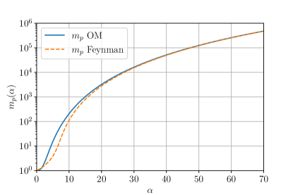
Figure 2: Effective mass as a function of $\alpha$ calculated by Feynman and our analytical formula in the logarithmic scale

Fig. 2 shows that this simple formula leads to all-coupling approximation for Feynman’s result which is connected with rather complicated variational calculations Feynman (1955a). Again one can calculate additional corrections to the effective mass if the high-order terms on the operator $\hat{H}_{1}$ will be taken into account in the equation (35).

V Conclusions

Simple algorithm for calculation of the polaron ground state and its characterisics in the entire range of the coupling constant is developed in the frameworks of the Schrödinger representation of the system. The method demands essentially less calculations in comparison with variational estimation of the functional integrals for this problem, and leads to the regular procedure for the calculation of the high-order corrections. It may be useful for other models in the quantum field theory.