Is the Gompertz family a good fit to your data?

Abstract

That data follow a Gompertz distribution is a widely used assumption in diverse fields of applied sciences, e.g., in biology or when analysing survival times. Since misspecified models may lead to false conclusions, assessing the fit of the data to an underlying model is of central importance. We propose a new family of characterisation-based weighted $L^{2}$-type tests of fit to the family of Gompertz distributions, hence tests for the composite hypothesis when the parameters are unknown. The characterisation is motivated by distributional transforms connected to Stein’s method of distributional approximation. We provide the limit null distribution of the test statistics in a Hilbert space setting and, since the limit distribution depends on the unknown parameters, we propose a parametric bootstrap procedure. Consistency of the testing procedure is shown. An extensive simulation study as well as applications to real data examples show practical benefits of the procedures: the first data set we analyse consists of lifetimes of fruitflies, the second has been synthetically generated from life tables for women born in Germany in 1948.

1 Introduction

The Gompertz distribution was first derived in [11] as a probability model for human mortality. It is widely accepted to describe the distribution of adult lifespans by actuaries and demographers. Indeed, as Prof. Dr. Oliver Kuß (German Diabetes Center and Heinrich-Heine University Düsseldorf) pointed out (personal communication): “In epidemiology and demography, the Gompertz distribution is used to model the distribution of lifetimes. It is widely accepted that, for ages of 40 years and older, the age at death is nearly perfectly Gompertz-distributed, as seen when comparing empirical (e.g., 5-year) mortality rates with those from a Gompertz fit.” Beside this prominent application, it is used in fields of applied sciences as biology, see [6], and gerontology, see [17], to describe the analysis of survival, in computer science for modeling failure rates, see [12], in hydrogen production of energy fuels, see [22, 31] or to describe the walk length of a random self-avoiding walk in the Erdős-Rényi random graph, see [29].

A first step for serious statistical inference using this model is to assess whether the observed data stems from a distribution being a member of the Gompertz family. Since, even if the assumption of an underlying Gompertz law is true, the true parameters are unknown, it is obvious that this fact has to be incorporated in a test deciding upon the fit of this family of distributions to the data. Hence, in contrast to a simple hypothesis of testing against one fixed Gompertz distribution (including the case that the parameters have been estimated in a first step and then are assumed to be known), a so called composite hypothesis has to be considered.

The literature for this goodness-of-fit testing problem is hitherto nearly non existent. The only exception is the article [18]. The authors provide a comparative simulation study for the classical Anderson-Darling test and some extension due to [25], as well as a correlation coefficient type test and a nested test against the truncated generalised extreme value distribution for the minimum. The cited article does not consider testing procedures for the composite case, since the authors first fit the parameters to a Gompertz law and then perform the simple hypothesis tests. No asymptotic theory for the testing procedures is derived. So we conclude that the composite case has hitherto not been treated in the literature.

In this article, we present new tests of fit to the Gompertz family of distributions based on a characterisation of the Gompertz law. The idea of using characterisations for deriving goodness-of-fit goes back to [20] and is the basis for powerful procedures; for details see [23]. The aim of this article is to propose the first characterisation based test of fit to the composite hypothesis that the data stems from (any) Gompertz law and provide asymptotic theory under the null hypothesis. Since the limit null distribution depends on the unknown shape parameter a parametric bootstrap procedure is presented and we provide the first comparative Monte Carlo simulation study for this setting. To be precise, let $GO(\eta,b)$ denote the Gompertz distribution defined by the probability density function

$$f(x;\eta,b)=b\eta\exp(\eta+bx-\eta e^{bx}),\quad x\geq 0,$$ (1)

where the rate $b>0$ is a scale parameter and $\eta>0$ is a shape parameter. The cumulative distribution function is given by

$$F(x;\eta,b)=1-\exp(-\eta(e^{bx}-1)),\quad x\geq 0,$$

and $F(x;\eta,b)=0$ otherwise. We write $\mathbf{\mbox{GO}}=\{GO(\eta,b):\eta,b>0\}$ for the family of Gompertz distributions, see [21], Chapter 10, for details on the parametric family GO. Let $X,X_{1},X_{2},\ldots$ be positive, independent and identically distributed (i.i.d.) random variables defined on a common probability space $(\Omega,\mathcal{A},\mathbb{P})$, and denote the distribution of $X$ by $\mathbb{P}^{X}$. We test the composite hypothesis

$$H_{0}:\;\mathbb{P}^{X}\in\mathbf{\mbox{GO}}$$ (2)

against general alternatives.

This paper is organised as follows. In Section 2, we introduce the family of Gompertz distributions, provide a Stein characterisation of these distributions, and propose a goodness-of-fit test statistic $T_{n}$ that is based on the Stein characterisation. In Section 3, we analyse the distribution of $T_{n}$ under the null hypothesis and develop a parametric bootstrap scheme for approximating this null distribution. In particular, we derive the asymptotic distribution of $T_{n}$ under the assumption of a Gompertz law using a Hilbert space framework, and we show that the parametric bootstrap procedure is well calibrated. This is followed by Section 4 where we consider the behaviour of the test statistic under alternatives: the procedure is consistent under a convergence assumption for the estimators. We present a competitive Monte Carlo simulation study under both the null and alternative hypothesis in Section 5 and compare the new tests to the classical empirical distribution based methods. The results indicate that the new test is a strong competitor to the classical procedures. The procedure is also applied to real data sets from biology and demography in Section 6. We conclude the paper by reflecting our findings and stating open problems in Section 7. All proofs and lengthy derivations are offered in the appendices.

2 Characterisation of the Gompertz law and the new test statistic

This article studies a test procedure for (2) based on a characterisation of the family of Gompertz distributions due to [3], Corollary 3. This type of characterisation is related to distributional characterisations in Stein’s method (for an introduction to the topic we refer to [7]) and the so-called density approach, see [19, 26]. For the sake of completeness, we state the characterisation, a proof is found in Appendix A.

Theorem 2.1.

Let $X$ be a positive random variable with cumulative distribution function $G$ and $\mathbb{E}|X|<\infty$. Define for $\eta,b>0$ the function $T^{X}:\mathbb{R}\rightarrow\mathbb{R}$

$$T^{X}(s)=\left\{\begin{array}[]{cc}\mathbb{E}\big{[}(\eta be^{bX}-b)\min\{X,s\}\big{]},&s>0,\\ 0,&s\leq 0.\end{array}\right.$$

Then $X\sim GO(\eta,b)$, if and only if $T^{X}\equiv G$ on $\mathbb{R}$.

In the following, we write $\stackrel{{\scriptstyle\mathcal{\mathbb{P}}}}{{\longrightarrow}}$ for convergence in probability, and $(\widehat{\eta}_{n},\widehat{b}_{n})$ for consistent estimators of $(\eta,b)$. We assume throughout that, for all considered distributions, we have $(\widehat{\eta}_{n},\widehat{b}_{n})\stackrel{{\scriptstyle\mathcal{\mathbb{P}}}}{{\longrightarrow}}(\eta_{0},b_{0})\in(0,\infty)^{2}$ as $n\rightarrow\infty$, i.e. if $X\sim GO(\eta,b)$, we have $(\widehat{\eta}_{n},\widehat{b}_{n})\stackrel{{\scriptstyle\mathcal{\mathbb{P}}}}{{\longrightarrow}}(\eta,b)$ as $n\rightarrow\infty$. In view of the scale invariance of the Gompertz family, we set $Y_{n,j}=\widehat{b}_{n}X_{j}$, $j=1,\ldots,n$ and assume that $\widehat{b}_{n}$ is a scale equivariant estimator of $b$, i.e., that we have

$$\widehat{b}_{n}(\beta X_{1},\ldots,\beta X_{n})=\widehat{b}_{n}(X_{1},\ldots,X_{n})/\beta$$

and that $\widehat{\eta}_{n}$ is scale invariant, i.e. that

$$\widehat{\eta}_{n}(\beta X_{1},\ldots,\beta X_{n})=\widehat{\eta}_{n}(X_{1},\ldots,X_{n})$$

holds for all $\beta>0$. This implies $\widehat{b}_{n}(Y_{n,1},\ldots,Y_{n,n})=1$, such that under $H_{0}$ the distribution of the random variables $Y_{n,j}$ should be close to a $GO(\eta,1)$ distribution. Hence, based on Theorem 2.1 we propose the weighted $L^{2}$-type statistic

$$T_{n}=n\int_{0}^{\infty}V_{n}^{2}(s)\,w(s)\;\mbox{d}s,$$

where

$$V_{n}(s)=\frac{1}{n}\sum_{j=1}^{n}(\widehat{\eta}_{n}e^{Y_{n,j}}-1)\min\{Y_{n,j},s\}-\frac{1}{n}\sum_{j=1}^{n}\mathbf{1}\{Y_{n,j}\leq s\},\quad s>0,$$ (3)

and $w(\cdot)$ is a continuous positive weight function, with

$$\int_{0}^{\infty}(s^{2}+1)w(s)\,ds<\infty,$$ (4)

and

$$n\int_{0}^{\infty}\big{|}w(\widehat{b}_{n}s)-w(s)\big{|}^{3}w^{-2}(s)\,ds\stackrel{{\scriptstyle\mathbb{P}}}{{\longrightarrow}}0,\qquad n\rightarrow\infty.$$ (5)

We reject the hypothesis $H_{0}$ for large values of $T_{n}$. Note that $T_{n}$ only depends on the rescaled data $Y_{n,j}$, $j=1,\ldots,n$, and as a consequence it is invariant due to scale transformations of the data, i.e. w.r.t. transformations of the form $x\mapsto\beta x$, $\beta>0$.

It is straightforward to show that for all $a>0$ the weight function $w_{a}(s)=\exp(-as)$, $s>0$, satisfies (4) and (5). Direct calculations lead to the numerical stable integration free representation

$$T_{n,a}= n\int_{0}^{\infty}V_{n}^{2}(s)w_{a}(s)\,ds$$

$$= \frac{2}{n}\sum_{0\leq i<j\leq n}\Bigg{[}\frac{G_{j}}{a^{3}}e^{-aY_{(i)}}\big{(}-aG_{i}Y_{(i)}-2G_{i}-a^{2}Y_{(i)}-a\big{)}$$

$$+\frac{1}{a^{2}}e^{-aY_{(j)}}\big{(}-G_{i}G_{j}Y_{(i)}-aG_{i}Y_{(i)}+G_{j}+a\big{)}+2G_{i}G_{j}\Bigg{]}$$

$$+\frac{1}{n}\sum_{j=1}^{n}\Bigg{[}\frac{1}{a^{3}}e^{-aY_{(j)}}\big{(}-2aG_{j}^{2}Y_{(j)}-2G_{j}^{2}-2a^{2}G_{j}Y_{(j)}+a^{2}\big{)}+2G_{j}^{2}\Bigg{]},$$

where $Y_{(j)}$ stands for the $j$th order statistic of $Y_{n,1},\ldots,Y_{n,n}$ and $G_{j}=\widehat{\eta}_{n}e^{Y_{(j)}}-1$, $j=1,\ldots,n$. Note that the proposed test is in the spirit of Stein goodness-of-fit tests, see [1] and the references therein for details on the general approach which is also applicable for other families of distributions. In [4] discrete analogs to Theorem 2.1 are derived and applied to testing the fit to families of discrete distributions.

3 Limit null distribution and bootstrap procedure

In this section, we derive the asymptotic distribution under the null hypothesis. Due to the $L^{2}$-structure of the test statistic, a convenient setting is the separable Hilbert space $\mathbb{H}=L^{2}([0,\infty),\mathcal{B},w(t){\rm d}t)$ of (equivalence classes of) measurable functions $f:[0,\infty)\rightarrow\mathbb{R}$ satisfying $\int_{0}^{\infty}|f(t)|^{2}\,w(t)\,{\rm d}t<\infty$. Here, $\mathcal{B}$ denotes the Borel sigma-field on $[0,\infty)$. The scalar product and the norm in $\mathbb{H}$ will be denoted by

$$\langle f,g\rangle_{\mathbb{H}}=\int_{0}^{\infty}f(t)g(t)\,w(t)\,{\rm d}t,\quad\|f\|_{\mathbb{H}}=\langle f,f\rangle_{\mathbb{H}}^{1/2},\quad f,g\in\mathbb{H},$$

respectively. In view of the scale invariance of $T_{n}$ we assume in the following that $X_{n,1},\ldots,X_{n,n}$ is a triangular array of rowwise i.i.d. random variables, and suppose $X_{n,1}\sim GO(\eta_{n},1)$ for a sequence of positive parameters $(\eta_{n})$, where $\lim_{n\rightarrow\infty}\eta_{n}=\eta>0$. In the following, we assume that the estimators $(\widehat{\eta}_{n},\widehat{b}_{n})$ allow linear representations

$$\sqrt{n}(\widehat{\eta}_{n}-\eta_{n}) =\frac{1}{\sqrt{n}}\sum_{j=1}^{n}\psi_{1}(X_{n,j},\eta_{n})+o_{\mathbb{P}}(1),$$ (6)

$$\sqrt{n}(\widehat{b}_{n}-1) =\frac{1}{\sqrt{n}}\sum_{j=1}^{n}\psi_{2}(X_{n,j},\eta_{n})+o_{\mathbb{P}}(1),$$ (7)

where $\psi_{1}$ und $\psi_{2}$ are measurable functions with

$$\mathbb{E}[\psi_{1}(X_{n,1},\eta_{n})]=0, \mathbb{E}[\psi_{2}(X_{n,1},\eta_{n})]=0,$$ (8)

$$\mathbb{E}[\psi_{1}^{2}(X_{n,1},\eta_{n})]<\infty, \mathbb{E}[\psi_{2}^{2}(X_{n,1},\eta_{n})]<\infty,$$ (9)

and

$$\lim_{n\rightarrow\infty}\mathbb{E}[\psi_{1}^{2}(X_{n,1},\eta_{n})]=\mathbb{E}[\psi_{1}^{2}(X,\eta)],\qquad\lim_{n\rightarrow\infty}\mathbb{E}[\psi_{2}^{2}(X_{n,1},\eta_{n})]=\mathbb{E}[\psi_{2}^{2}(X,\eta)].$$ (10)

Here and in the following $o_{\mathbb{P}}(1)$ stands for a term that converges to 0 in probability. An example for $(\widehat{\eta}_{n},\widehat{b}_{n})$ satisfying these assumptions are the maximum-likelihood estimators. This fact can be proved by straightforward calculations showing the existence of the inverse Fisher information matrix and applying Theorem 5.39 in [30].

Theorem 3.1.

Under the triangular array $X_{n,1},\ldots,X_{n,n}$, we have

$$T_{n}=n\|V_{n}\|_{\mathbb{H}}^{2}\stackrel{{\scriptstyle\mathcal{D}}}{{\longrightarrow}}\|\mathcal{W}\|_{\mathbb{H}}^{2},\quad n\rightarrow\infty,$$

where $\mathcal{W}$ is a centred Gaussian random element in $\mathbb{H}$ having covariance kernel

$$\mathcal{K}_{\eta}(s,t)= (s-2)F(s;\eta,1)+s(1-t)F(t;\eta,1)+2\mathbb{E}\big{[}X\mathbf{1}\{X\leq s\}\big{]}+\mathbb{E}\big{[}X^{2}\mathbf{1}\{X\leq s\}\big{]}$$

$$+\mathbb{E}\big{[}X\mathbf{1}\{X\leq t\}\big{]}+\mathbb{E}\big{[}R(s;\eta)r(t;\eta)\big{]}+\mathbb{E}\big{[}R(t;\eta)r(s;\eta)\big{]}+\mathbb{E}\big{[}r(s;\eta)r(t;\eta)\big{]}$$

for $0<s\leq t<\infty$, where $X\sim GO(\eta,1)$ and

$$R(s;\eta)= (\eta Xe^{X}-X-1)\mathbf{1}\{X\leq s\}+s(\eta e^{X}-1)\mathbf{1}\{X>s\},$$

$$r(s;\eta)= \psi_{1}(X,\eta)\frac{1}{\eta}\big{(}1+\mathbb{E}\big{[}X\mathbf{1}\{X\leq s\}\big{]}\big{)}+\psi_{2}(X,\eta)\big{(}1+\mathbb{E}\big{[}X\big{]}+\mathbb{E}\big{[}X\mathbf{1}\{X\leq s\}\big{]}+\mathbb{E}\big{[}X^{2}\mathbf{1}\{X\leq s\}\big{]}\big{)}.$$

The distribution of $\|\mathcal{W}\|_{\mathbb{H}}^{2}$ is known to have the equivalent representation $\sum_{j=1}^{\infty}\lambda_{j}(\eta)N_{j}^{2}$, where $N_{1},N_{2},\ldots$ are independent, standard normally distributed random variables, and $\lambda_{1}(\eta),\lambda_{2}(\eta),\ldots$ is the decreasing series of non-zero eigenvalues of the integral operator

$$K:\mathbb{H}\rightarrow\mathbb{H},\quad f\mapsto Kf(\cdot)=\int_{0}^{\infty}\mathcal{K}_{\eta}(\cdot,t)f(t)\,w(t)\,\mbox{d}t.$$

This operator obviously depends on the true unknown parameter $\eta>0$. To calculate the eigenvalues $\lambda$ of $\mathcal{K}$, one has to solve the homogeneous Fredholm integral equation of the second kind

$$\int_{0}^{\infty}\mathcal{K}_{\eta}(x,t)f(t)\,w(t)\,\mbox{d}t=\lambda f(x),\quad x>0,$$ (11)

see, e.g., [16]. Due to the complexity of the covariance kernel, it seems hopeless to find explicit solutions of (11) and hence formulae for the eigenvalues. Although numerical and stochastic approaches to approximate the eigenvalues can be found in the literature, see for example [5, 10, 27], the complexity of $\mathcal{K}_{\eta}$ indicates that even these approaches are hard to apply. Furthermore, since the true parameter $\eta$ is unknown in practice, the limiting null distribution cannot be used to derive critical values of the test. A solution to this problem is provided by a parametric bootstrap procedure as suggested in [15] and which is stated as follows:

1. Compute $\widehat{\eta}_{n}=\widehat{\eta}_{n}(X_{1},\ldots,X_{n})$.

2. Conditionally on $\widehat{\eta}_{n}$ and $\widehat{b}_{n}=1$, simulate $B$ bootstrap samples $X_{j,1}^{*},\ldots,X_{j,n}^{*}$, i.i.d. from $GO\left(\widehat{\eta}_{n},1\right)$, and compute $T_{n,j}^{*}=T_{n}(X_{j,1}^{*},\ldots,X_{j,n}^{*})$, $j=1,\ldots,B$.

3. Denote by

   $$H_{n,B}^{*}(s)=\frac{1}{B}\sum_{j=1}^{B}\mathbf{1}\{T_{n,j}^{*}\leq s\},\qquad s>0,$$

   the empirical distribution function of $T_{n,1}^{*},\ldots,T_{n,B}^{*}$ and derive the empirical $(1-\alpha)$-quantile $c_{n,B}^{*}(\alpha)$.

4. Reject the hypothesis (2) at level $\alpha$ if $T_{n}(X_{1},\ldots,X_{n})>c_{n,B}^{*}(\alpha)$.

Note that for each computation of $T_{n,j}^{*}$, parameter estimation has to be done separately for each $j$ and clearly the tests depend on the rescaled bootstrap data. The following theorem gives the final justification for the right-tailed test procedure for testing $H_{0}$ based on the test statistic $T_{n}$.

Theorem 3.2.

Let $X\sim GO(\eta_{n},1)$, where $(\eta_{n})$ is again a positive sequence with $\lim_{n\rightarrow\infty}\eta_{n}=\eta>0$ and $X_{1},\ldots,X_{n}$ be i.i.d copies of $X$. Further denote by $H_{n,B}^{*}$ and $c_{n,B}^{*}$ the quantities from the bootstrap procedure. Then, we have

$$\mathbb{P}_{\eta}\big{(}T_{n}>c_{n,B}^{*}(\alpha)\big{)}\longrightarrow\alpha,\qquad\text{as }n,B\rightarrow\infty.$$

4 Consistency

In this section, we assume that $X$ is a positive, non-degenerate random variable with an arbitrary distribution such that $\mathbb{E}[X]<\infty$ and $\mathbb{E}[X\exp(X)]<\infty$. In view of the scale invariance of $T_{n}$, we assume $b_{0}=1$, i.e. that $(\widehat{\eta}_{n},\widehat{b}_{n})\stackrel{{\scriptstyle\mathcal{\mathbb{P}}}}{{\longrightarrow}}(\eta_{0},1)$, $\eta_{0}>0$, for $n\rightarrow\infty$.

Remark 4.1.

Note that, under certain regularity conditions, maximum likelihood estimators in misspecified models are known to be consistent for the minimiser of a Kullback-Leibler information criterion; see Theorem 2.2 in [32]. In the following, we will assume that such a consistency holds.

Theorem 4.2.

Let $X_{1},\ldots,X_{n}$ be i.i.d. copies of $X$. Then

$$\frac{T_{n}}{n}\stackrel{{\scriptstyle\mathbb{P}}}{{\longrightarrow}}\Delta_{\eta_{0}},\quad n\rightarrow\infty,$$

where $\Delta_{\eta_{0}}=\|\Delta_{\eta_{0}}^{*}\|_{\mathbb{H}}^{2}$ and $\Delta_{\eta_{0}}^{*}(s)=\mathbb{E}\big{[}(\eta_{0}e^{X}-1)\min\{X,s\}\big{]}-\mathbb{P}(X\leq s),\quad s>0$.

The following corollary shows that the parametric bootstrap testing procedure based on $T_{n}$ is consistent against a broad class of alternatives.

Corollary 4.3.

Under the standing assumptions with the notations from Section 3, we have if $\mathbb{P}^{X}\not\in\mathbf{\mbox{GO}}$

$$\mathbb{P}\big{(}T_{n}>c_{n,B}^{*}(\alpha)\big{)}=1,\qquad n,B\rightarrow\infty.$$

5 Simulation study

We assess the practical usefulness of the new test with the help of an extensive simulation study. We chose the significance level $\alpha=5\%$, sample sizes $n=20,50,100$, and repeated each test for each simulation scenario 10,000 times, where each test was based on 2,000 parametric bootstrap iterations. The test was applied for several choices of the tuning parameter, $a\in\{0.1,0.25,0.5,0.75,1,1.5,2,3,5,10\}$. Additionally, we considered the following competitor goodness-of-fit tests, which are also scale-invariant because they are based on the empirical distribution function $\widehat{F}_{n}$ of the re-scaled data, $Y_{j}=\widehat{b}_{n}X_{j}$:

(Kolmogorov-Smirnov) $$\mbox{KS}=\sup_{x}|\widehat{F}_{n}(x)-F(x;\widehat{\eta}_{n},1)|,$$

(Anderson-Darling) $$\mbox{AD}=\int_{-\infty}^{\infty}\frac{(\widehat{F}_{n}(x)-F(x;\widehat{\eta}_{n},1))^{2}}{F(x;\widehat{\eta}_{n},1)(1-F(x;\widehat{\eta}_{n},1))}dF(x;\widehat{\eta}_{n},1)$$

(Cramér-von Mises) $$\mbox{CM}=\int_{-\infty}^{\infty}(\widehat{F}_{n}(x)-F(x;\widehat{\eta}_{n},1))^{2}dF(x;\widehat{\eta}_{n},1)$$

(Watson) $$\mbox{WA}=\mbox{CM}-n\Big{(}\frac{1}{n}\sum_{j=1}^{n}F(Y_{j};\widehat{\eta}_{n},1)-\frac{1}{2}\Big{)}^{2}.$$

All of these competitor tests were conducted based on the same parametric bootstrap procedure as described in Section 3. For this we used the maximum likelihood parameter estimators; see Appendix B for technical details about the practical implementation, also about cases when no maximiser could be found.

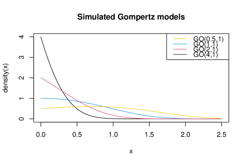
Figure 1: Density functions of Gompertz distributions with scale parameter $b=1$ and shape parameters $\eta=$ 0.5 (yellow), 1 (blue), 2 (red), 4 (black).

The sizes of the tests under the null hypothesis were simulated based on various underlying Gompertz distributions, $GO(0.5,1),GO(1,1),GO(2,1),GO(4,1)$; recall that the tests are scale-invariant, which is why we only let the shape parameter vary. Figure 1all illustrates the considered Gompertz distributions in terms of their densities. In order to compare the tests’ power behaviour under the alternative hypothesis, we simulated data according to the non-Gompertz distributions with non-negative support summarised in Table 1.

distribution	density (in $x>0$)
lognormal $LN(\sigma),\sigma=0.5,1,$	${\exp(-\frac{(\log x)^{2}}{2\sigma^{2}})}/(\sqrt{2\pi}\sigma x)$,
Gamma $\Gamma(k),k=1,2,3$	${x^{k-1}\exp(-x)}/{\Gamma(k)}$,
inverse Gaussian $IG(\mu,\lambda),\mu=1,\lambda=1,3$	$\sqrt{\frac{\lambda}{2\pi x^{3}}}\exp\Big{(}-\frac{\lambda(x-\mu)^{2}}{2\mu^{2}x}\Big{)}$,
Weibull $W(k),k=0.5,3$	$\frac{k}{\lambda}\Big{(}\frac{x}{\lambda}\Big{)}^{k-1}\exp\Big{(}-\Big{(}\frac{x}{\lambda}\Big{)}^{k}\Big{)}$,
Uniform $U(0,5)$	$0.2\cdot 1_{(0,5)}(x)$,
Power $Pow(\nu),\nu=1,2,4$	$x^{\tfrac{1}{\nu}-1}/\nu\ \cdot\ 1\{0\leq x\leq 1\}$,
shifted Pareto $SP(\nu),3,5,10$	$\nu(x+1)^{-\nu-1}$,
linearly increasing failure rate $LF(\nu),\nu=3,5,10$	$\nu(x+1)\exp\Big{(}\frac{1-\nu^{2}(x+1)^{2}}{2\nu}\Big{)}$,
$GO(1)$-$\Gamma(5)$-mixture $Mix(p),p=0.1,0.25,0.5,0.75$	$p\cdot\exp(1+x-e^{x})+(1-p)\cdot{x^{4}\exp(-x)}/{\Gamma(5)}$.

Table 1: Non-Gompertz distributions considered in the simulation study.

Note that $\Gamma(1)$ is an exponential distribution ($Exp$), $Pow(1)$ is a uniform distribution, and, indeed, $LF(a)$ has the linearly increasing failure (or hazard) rate $x\mapsto a(x+1)$.

	true	proposed Goodness-of-fit test; tuning parameter $a=$										classical tests				not found
n	distr.	$0.1$	$0.25$	$0.5$	$0.75$	$1$	$1.5$	$2$	$3$	$5$	$10$	AD	KS	CM	WA	$\widehat{b}_{n}$	$\widehat{b}_{n}^{*}$
20	$GO(0.5,1)$	2	3	5	6	6	6	6	6	5	5	5	5	5	5	1	1
50		4	4	5	5	6	6	6	5	5	4	5	5	5	5	0	0
100		4	4	5	5	5	5	5	5	5	5	5	5	5	5	0	0
20	$GO(1,1)$	2	3	4	5	5	6	6	6	6	6	5	5	5	5	3	3
50		3	4	4	4	5	5	6	6	5	5	5	5	5	5	1	2
100		4	4	5	5	5	5	6	6	6	5	5	5	5	5	0	1
20	$GO(2,1)$	2	3	3	4	4	5	6	6	6	6	4	4	4	5	6	7
50		3	3	3	3	4	4	5	5	6	5	5	5	5	5	5	6
100		3	3	3	4	4	5	5	5	6	6	5	5	5	5	2	3
20	$GO(4,1)$	3	3	4	4	4	5	6	6	6	6	4	4	4	4	11	10
50		3	3	3	3	3	4	4	5	6	6	4	4	4	5	10	12
100		3	3	3	3	3	4	4	5	6	6	5	4	4	5	7	10

Table 2: Simulated rounded rejection probabilities (in %) under the null hypothesis. The considered classical tests are Anderson-Darling (AD), Komogorov-Smirnov (KS), Cramér-von Mises (CM), Watson (WA). The last two columns contain the frequency (in %) of how often the maximum likelihood estimators $\widehat{b}_{n}$ and the parametric bootstrap counterpart $\widehat{b}_{n}^{*}$ could not be found.

	true	proposed Goodness-of-fit test; tuning parameter $a=$										classical tests				not found
n	distr.	$0.1$	$0.25$	$0.5$	$0.75$	$1$	$1.5$	$2$	$3$	$5$	$10$	AD	KS	CM	WA	$\widehat{b}_{n}$	$\widehat{b}_{n}^{*}$
20	$LN(0.5)$	40	47	54	58	60	58	54	45	33	18	53	45	53	54	1	1
50		95	96	97	98	98	98	98	97	93	73	97	93	95	95	0	0
100		100	100	100	100	100	100	100	100	100	100	100	100	100	100	0	0
20	$LN(1)$	9	10	10	10	11	12	11	11	11	10	15	17	19	19	22	10
50		13	12	14	14	15	15	15	15	15	15	41	32	40	44	34	15
100		15	15	16	18	18	17	17	17	17	17	78	55	67	75	42	21
20	$\Gamma(1)$	5	6	5	6	6	7	7	7	7	6	7	7	7	6	15	10
50		5	5	6	6	6	6	6	7	6	5	7	7	6	6	19	12
100		6	5	5	6	6	6	6	6	5	5	6	6	6	6	24	16
20	$\Gamma(2)$	4	5	7	10	11	14	15	16	14	11	11	12	14	15	1	2
50		25	27	31	34	37	41	43	45	46	45	42	32	39	39	0	0
100		61	62	65	68	71	74	76	79	82	84	79	63	71	70	0	1
20	$\Gamma(3)$	15	18	23	27	29	30	28	24	18	10	23	21	26	26	0	0
50		62	65	69	72	74	75	76	75	72	58	71	57	65	65	0	0
100		94	94	95	96	97	98	98	98	98	97	97	90	94	93	0	0
20	$IG(1,1)$	6	7	8	9	10	12	13	15	17	18	18	18	22	26	14	9
50		9	10	12	15	16	20	24	29	36	45	73	57	62	70	16	11
100		19	17	19	22	24	29	32	38	45	51	99	96	96	98	20	15
20	$IG(1,3)$	31	37	46	52	55	57	55	49	38	23	50	44	51	52	2	1
50		93	94	96	97	97	97	98	97	96	86	98	93	95	95	1	1
100		100	100	100	100	100	100	100	100	100	100	100	100	100	100	0	0
20	$W(0.5)$	19	21	21	22	21	23	24	24	25	26	97	91	93	84	51	15
50		20	21	20	21	23	25	28	35	44	54	100	100	100	100	53	19
100		19	20	20	21	23	26	29	39	69	74	100	100	100	100	53	23
20	$W(3)$	15	17	19	17	14	7	3	1	0	0	14	12	15	15	0	0
50		47	48	49	48	45	34	21	9	2	0	40	26	35	35	0	0
100		80	81	82	83	82	77	69	52	26	1	74	50	63	62	0	0

Table 3: Simulated rounded rejection probabilities (in %) under alternative hypotheses with distributions: lognormal ($LN$), gamma ($\Gamma$), inverse Gauss ($IG$), Weibull ($W$), uniform ($U$). The considered classical tests are Anderson-Darling (AD), Komogorov-Smirnov (KS), Cramér-von Mises (CM), Watson (WA). The last two columns contain the frequency (in %) of how often the maximum likelihood estimator $\widehat{b}_{n}$ and the parametric bootstrap counterpart $\widehat{b}_{n}^{*}$ could not be found.

The results of the simulation study are shown in Tables 3–4. The last two columns therein indicate how often the maximum likelihood estimator $\widehat{b}_{n}$ or its bootstrap counterpart $\widehat{b}_{n}^{*}$ could not be found. This happened quite rarely under the null hypothesis, with a higher chance for larger shape parameters of the Gompertz distribution (up to 12% of the iterations for $\eta=4$). Under non-Gompertz distributions, these percentages strongly vary from case to case, even within the same family of distributions: e.g., for Weibull distributions from not at all (Weibull parameter equal to 3) to about 53% (for $\widehat{b}_{n}$, when the parameter equaled 0.5).

Table 3 displays the results in terms of empirical rejection rates under the null hypothesis. We observed only little variation with a change of sample sizes; most of the proposed tests for $a\geq 1.5$ and all of the classical tests exhibited rejection rates very close to 5%. However, for tuning parameters $a\leq 1$, most of the proposed tests tend to be conservative with rejection rates going down to 3%, in some few cases even 2%.

	true	proposed Goodness-of-fit test; tuning parameter $a=$										classical tests				not found
n	distr.	$0.1$	$0.25$	$0.5$	$0.75$	$1$	$1.5$	$2$	$3$	$5$	$10$	AD	KS	CM	WA	$\widehat{b}_{n}$	$\widehat{b}_{n}^{*}$
20	$Pow(1)$	9	11	14	15	15	14	13	12	11	10	14	9	11	11	0	1
50		35	36	36	36	33	29	25	21	19	16	35	21	28	28	0	0
100		73	72	70	66	63	55	48	41	34	26	69	43	58	58	0	0
20	$Pow(2)$	6	7	9	12	15	20	23	28	34	40	57	30	35	37	12	11
50		21	20	23	29	33	42	48	57	64	71	89	61	71	74	9	11
100		61	53	55	62	66	73	78	83	86	88	99	91	96	97	6	9
20	$Pow(4)$	16	15	14	15	15	17	17	17	15	11	99	93	94	92	49	20
50		18	16	14	15	15	16	17	18	17	10	100	100	100	100	52	23
100		20	16	15	16	16	19	20	21	19	13	100	100	100	100	52	25
20	$SP(3)$	12	12	12	13	13	14	14	14	11	8	31	29	31	20	36	16
50		16	16	16	18	19	19	20	19	17	11	54	50	55	35	46	20
100		20	18	19	21	23	24	24	24	21	16	77	72	78	56	51	23
20	$SP(5)$	9	9	9	9	10	10	10	10	9	7	17	16	18	11	31	17
50		12	11	12	12	13	13	13	13	11	7	28	25	29	16	40	22
100		15	13	14	15	16	17	16	16	14	9	43	39	44	25	47	24
20	$SP(10)$	7	7	8	8	7	8	8	8	7	6	9	10	10	7	25	16
50		8	8	8	8	8	8	9	9	8	6	13	12	13	9	33	22
100		10	9	9	9	10	10	10	10	9	6	17	15	18	11	38	24
20	$LF(3)$	3	3	4	5	6	7	7	7	6	5	5	6	6	6	3	4
50		5	5	6	7	8	9	9	9	8	6	7	7	8	8	2	2
100		11	11	12	13	13	14	13	13	12	10	11	10	11	12	0	1
20	$LF(5)$	3	4	5	5	6	7	7	6	5	4	5	6	6	7	2	3
50		7	8	9	10	10	11	11	11	9	7	8	8	10	10	1	2
100		16	17	17	18	18	19	19	18	16	13	16	14	16	16	0	0
20	$LF(10)$	4	4	6	7	8	8	8	7	5	3	6	7	7	8	2	2
50		10	11	12	14	14	15	14	13	11	7	12	11	13	13	0	1
100		24	25	26	27	27	28	27	26	24	18	24	19	23	23	0	0
20	$Mix(0.1)$	10	12	15	16	16	15	13	10	8	7	14	13	15	15	0	0
50		35	36	37	38	38	36	32	26	16	9	34	32	37	36	0	0
100		64	65	65	66	66	64	60	51	33	13	62	59	65	64	0	0
20	$Mix(0.25)$	5	7	10	13	16	19	21	23	25	24	21	15	15	16	0	1
50		16	19	23	28	32	37	40	44	46	44	40	32	33	33	0	0
100		40	44	50	56	61	67	70	73	73	68	69	59	63	64	0	0
20	$Mix(0.5)$	9	11	13	15	18	22	24	27	30	32	45	44	48	49	19	9
50		20	20	23	27	30	34	38	43	48	53	85	84	89	90	19	11
100		34	26	28	33	36	42	47	53	59	63	99	99	100	100	17	14
20	$Mix(0.75)$	18	17	18	19	19	19	18	17	13	9	56	59	64	56	47	15
50		21	19	20	23	23	24	23	22	17	9	95	95	97	95	52	19
100		21	18	18	23	23	24	23	22	19	16	100	100	100	100	53	23

Table 4: Simulated rounded rejection probabilities (in %) under alternative hypotheses with distributions: power ($Pow$), shifted Pareto ($SP$), linear failure ($LF$), mixture ($Mix$). The considered classical tests are Anderson-Darling (AD), Komogorov-Smirnov (KS), Cramér-von Mises (CM), Watson (WA). The last two columns contain the frequency (in %) of how often the maximum likelihood estimator $\widehat{b}_{n}$ and the parametric bootstrap counterpart $\widehat{b}_{n}^{*}$ could not be found.

Let us now compare the power results of the proposed and the classical tests; the simulation results are shown in Tables 3 and 4. We generally noticed that the proposed tests are in most cases good competitors of the classical tests in many scenarios; at least for some choices of $a$ their rejection rates were close to or slightly greater than those of the classical tests. This concerns the following distributions: $LN(0.5)$, $\Gamma(k),k=1,2,3$, $IG(1,3)$, and $W(3)$ from Table 3 as well as the uniform distribution $Pow(1)$, $LF(\nu),\nu=3,5,10$, and the mixture distributions $Mix(p),p=0.1,0.25$ from Table 4. In contrast to that, we also observed that the classical tests clearly outperform the proposed tests in some of the remaining scenarios, e.g. for the underlying distributions $LN(1)$, $IG(1,1)$, $W(0.5)$ from Table 3 and $Pow(2),Pow(4)$, $SP(3),SP(5)$, $Mix(0.5)$, and $Mix(0.75)$ from Table 4. It seems that all of the cases go hand in hand with a high chance that the maximum likelihood estimator could not be found.

Most choices of the tuning parameter $a$ resulted in a similar simulated power of the proposed tests; notable exceptions from this can be found for the distributions $LN(0.5)$ (for $n=20$), $\Gamma(2)$, $\Gamma(3)$, $IG(1,1)$, $W(k)$, $Pow(1)$, $Pow(2)$, $Mix(p)$. The classical tests exhibited a similar power in most scenarios.

All in all, our proposed tests often perform well compared to the classical tests – but a good choice of the tuning parameter $a$ is of the essence under some alternatives. Also, if the maximum likelihood estimator for the scale parameter $b$ could not be computed with a relatively high probability, the proposed tests performed suboptimal.

6 Real data example

In this section, we apply the goodness-of-fit tests to two different data sets related to lifetimes related to fruitflies and to females born in Germany in 1948 (generated from a life table). We chose the significance level $\alpha=5\%$ for all conducted tests.

6.1 Lifetimes of fruitflies

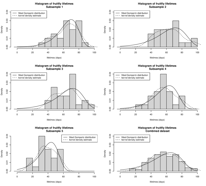
Figure 2: Lifespan (in days) of the fruitflies with separate plots for all subsamples and the complete data set; comparison of histograms, kernel density estimators (default choices in R), and fitted Gompertz distributions.

The first data set we are about to analyse consists of 125 recorded lifetimes of male fruitflies – a data set which is publicly available. The data resulted from five different groups of male fruitflies of size 25 each; in the different experimental groups varying types and numbers of mating partners. [24] argued that “increasing sexual activity reduces longevity in the male fruitfly”. For some educational aspects of the data and their analysis, we refer to [13, 14].

At first, we considered the longevity values of the complete data set, i.e. including the measurements from all of the five subgroups. Figure 2 (panel on the bottom-right) illustrates the data set in a histogram which is compared to a nonparametric kernel density estimator and the fitted parametric Gompertz distribution. The histogram and the kernel density estimator suggest a distribution with at least two modes rather than a unimodal distribution such as the fitted Gompertz distribution. One reason for the multimodality could be the heterogeneity of the lifetime values in the different groups: in the other panels of the same Figure, we can see that the location parameters of Subsamples 4 and 5 differ from those of Subsamples 1 to 3.

The $p$-values of the applied goodness-of-fit tests based on 2,000 resampling iterations can be found in Table 5. It is apparent that, for the complete data set, the proposed test rejects the null hypothesis of Gompertz distributed data for most values of the tuning parameter $a$ – to be more precise: for all $a\leq 2$. Also, nearly all of the classical tests arrive at the same result. Apart from this, almost none of the tests produced a significant outcome when applied separately to the subsamples. These results could have the following reasons: first, it is not surprising that the power of the tests increase together with the sample size, and the combined data set ($n=125$) is much larger than each of the subsamples ($n=25$). Second, it is possible that the combination of all five subsamples with most likely different underlying distributions resulted in a sample which cannot be appropriately described by any Gompertz distribution: the mixture of different Gompertz distributions is not a Gompertz distribution. Also comparing the Gompertz distribution fitted to the combined data set with the kernel density estimator clearly reveals a discrepancy: the density estimate looks almost symmetric and bimodal whereas the fitted Gompertz distribution is left-skewed and unimodal.

As a concluding remark regarding the analysis of these data, we would like to point out that the proposed tests did not produce many surprises when compared to the classical tests.

	proposed Goodness-of-fit test; tuning parameter $a=$										classical tests
(sub)sample	$0.1$	$0.25$	$0.5$	$0.75$	$1$	$1.5$	$2$	$3$	$5$	$10$	AD	KS	CM	WA
complete	$<\!\textbf{1}$	$<\!\textbf{1}$	$<\!\textbf{1}$	$<\!\textbf{1}$	$<\!\textbf{1}$	2	4	10	16	36	$<\!\textbf{1}$	5	4	4
1	71	65	55	49	47	48	51	53	48	44	52	49	50	47
2	6	5	5	7	10	27	44	56	55	51	8	27	15	17
3	6	6	6	8	13	31	47	57	54	49	9	22	15	17
4	28	27	30	36	44	57	62	60	54	49	22	14	27	28
5	42	39	35	35	35	43	49	54	56	53	33	9	28	28

Table 5: $p$-values (in %) of all tests applied to the fruitflies data set; rounded to full percentages. Significant results (in view of the significance level $\alpha=5\%$) are printed in bold-type.

6.2 Data generated from a life table for females born in Germany in 1948

The second type of data sets we are going to analyse is based on life tables provided by the Federal Statistical Office of Germany (Statistisches Bundesamt in Wiesbaden, Germany) published on September 29, 2020, which is publicly available. Based on the instantaneous hazard rates for females born in 1948 in Germany ($q_{x}$ in the second column on pp. 439-440 of the pdf file that includes the life tables), we reconstructed the underlying probability mass function; see Appendix C for more details. Based on these, we could generate data with the help of a multinomial distribution where the probability parameters are equal to the just-mentioned probability mass function. Because of the early peak due to a relatively high infant mortality and because the hazard rates for the ages above 100 years were aggregated, we decided to crop the distribution to the spans of (i) 10 and 99 years and (ii) 40 and 99 years. Our idea was to check whether the goodness-of-fit tests are able to detect any deviance from the Gompertz distribution family and whether the fit to some Gompertz distribution is reasonably well if the lifetimes are restricted to all deaths between the ages of 40 and 99, similarly as was motivated in Section 1.

Based on each of these two truncated distributions, we artificially generated data sets of sizes 20, 50, 100, and 1,000. Table 6 contains the $p$-values of the conducted tests. Let us first focus on the lifetimes truncated to 10 to 99 years. For $n\leq$ 100, none of the classical tests rejected $H_{0}$ but all of them rejected $H_{0}$ for $n=$ 1,000. None of the proposed tests rejected $H_{0}$ for $n=20,50$ either. For $n=$ 100, the outcomes of the proposed tests do not all agree: all tests with $a\leq 0.75$ rejected $H_{0}$ but no test with $a\geq 1$ rejected $H_{0}$. For $n=$ 1,000, this threshold for the tuning parameter $a$ is shifted to $a\leq 2$ and $a\geq 3$.

Next, for the lifetimes truncated to 40 to 99 years, we found a similar pattern for the proposed tests, although now fewer of them rejected $H_{0}$: those based on $a\geq 0.5$ did not reject $H_{0}$ for $n=100$. On the other hand, all of the classical tests rejected $H_{0}$ for that sample size. For $n=$ 1,000, we got similar results, except that now all proposed tests with $a$ up to 1 rejected the null hypothesis; for greater $a$ it was not rejected. The Kolmogorov-Smirnov test is the only one which rejected $H_{0}$ for all considered sample sizes.

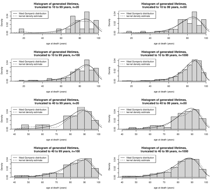
Figure 3: Histograms of artificially generated lifetimes (in years) of women born in Germany in 1948, a kernel density estimator (dashed lines; default values in R), and fitted Gompertz distributions (straight lines); for different truncations of the lifetime distributions: 10 to 99 year (upper half) and 40 to 99 (lower half). The same seed is used to generate all eight data sets.

Some concluding remarks from the perspective of the proposed tests: we see our earlier assumption confirmed by most tests that the lifetimes above 40 are approximately Gompertz-distributed; at least if the tuning parameter $a$ is not overly small. As the sample size increases to 1,000, more and more tests tend to reject the Gompertz family model which is natural in view of their increasing power and the wrongness of all models. However, if the truncation is made to the lifetimes between 10 and 99 years, the proposed tests reject $H_{0}$ more readily, indicating that the Gompertz family model might not be appropriate for the general lifetime distribution; this remark certainly all the more applies to the completely unrestricted distribution in which a high infant mortality could be observed (not depicted).

truncation	sample	proposed Goodness-of-fit test; tuning parameter $a=$										classical tests
to years	size	$0.1$	$0.25$	$0.5$	$0.75$	$1$	$1.5$	$2$	$3$	$5$	$10$	AD	KS	CM	WA
10 to 99	20	18	12	8	7	6	5	5	6	11	39	55	79	74	76
	50	15	12	11	11	11	12	11	12	22	44	55	62	76	82
	100	1	1	2	3	6	10	12	12	26	45	6	7	16	24
	1,000	$<$1	$<$1	$<$1	$<$1	$<$1	$<$1	$<$1	6	9	39	$<$1	$<$1	$<$1	$<$1
40 to 99	20	10	11	14	21	25	28	28	39	39	39	16	4	18	19
	50	16	18	24	30	36	38	37	45	43	43	17	3	12	13
	100	2	3	5	9	15	25	31	47	45	44	2	$<$1	3	3
	1,000	$<$1	$<$1	$<$1	$<$1	$<$1	12	33	66	58	52	$<$1	$<$1	$<$1	$<$1

Table 6: $p$-values (in %) of all tests applied to the data sets generated based on the (truncated) life tables; rounded to full percentages. Significant results (in view of the significance level $\alpha=5\%$) are printed in bold-type.

7 Discussion and outlook

In the present paper, we demonstrated how a Stein characterisation for the Gompertz distribution family can be used to develop a parametric bootstrap-based goodness-of-fit test for the composite null hypothesis. In our simulation study and the real data analyses, we have used the maximum likelihood estimators of the parameters of the Gompertz distribution. Other choices of parameter estimators could also be covered by the developed theory as long as they exhibit an asymptotically linear structure, for more information on the influence of parameter estimation techniques on the power of goodness-of-fit tests see [9]. This could potentially solve the issue of the suboptimal power seen in Tables 3 and 4 whenever there was a high probability that the maximum likelihood estimator for the scale parameter $b$ could not be found. Other than that, the proposed test revealed a good control of the type-I error probability across multiple underlying Gompertz distributions and a satisfactory power behaviour under many considered alternative hypotheses, also when compared to classical competitor tests. Still, the choice of the tuning parameter $a$ is crucial for obtaining a reliable test. In general, if no further information is available, intermediate choices of $a$ close to $1.5$ seem to be safest. Another possibility to solve this issue is to combine the proposed test with an adaptive selection procedure; see for instance [28] for a bootstrap-based approach. It should be noted that the additional bootstrap layer would significantly increase the computational complexity of the test procedure.

Finally, in view of applications to medical time-to-event data, another important extension of the proposed test would involve the handling of censored data. The difficulties in this connection are two-fold: firstly, the test statistic would need to involve the Kaplan-Meier estimator of the re-scaled observations instead of the empirical cumulative distribution function and, in particular, the expectation given in the Stein characterisation needed to be replaced by another estimator for which there is no standard approach. Secondly, the maximum likelihood estimators of the Gompertz distribution parameters would change. The large sample properties of the resulting test statistic could potentially be established by means of adaptations of techniques from survival analysis.

Conflict of interest statement

Both authors declare that there are no financial or commercial conflicts of interest.

Appendix

Appendix A Proofs

First we show a Stein-type characterisation of the Gompertz distribution, which is a special case of the so called density approach in Stein’s method, see [26], Proposition 1.4. The proof of Lemma A.1 follows the lines of proof of Theorem 1 in [2] and is hence omitted.

Lemma A.1.

A positive random variable $X$ is $GO(\eta,b)$, $\eta,b>0$, distributed, if and only if

$$\mathbb{E}\big{[}g^{\prime}(X)+\big{(}-\eta be^{bX}+b\big{)}g(X)\big{]}=0$$

holds for all functions $g\in\mathcal{G}$, where

$$\mathcal{G}=\big{\{}g:(0,\infty)\rightarrow\mathbb{R}| \;g\text{ is differentiable},g^{\prime}(x)\text{ and }\big{(}\eta be^{bx}-b\big{)}g(x)\text{ are bounded, and}$$

$$\lim_{x\downarrow 0}g(x)=\lim_{x\downarrow 0}g(x)f(x)=\lim_{x\rightarrow\infty}g(x)f(x)=0\big{\}},$$

and $f$ represents the probability density function of $GO(\eta,b)$ in (1).

Proof of Theorem 2.1. First assume that $X\sim GO(\eta,b)$. With $f(x)=f(x;\eta,b)$ as in (1) we have

$$\mathbb{E}\big{[}(\eta be^{bX}-b)\mathbf{1}\{X>s\}\big{]} =\int_{0}^{\infty}(\eta be^{bx}-b)\mathbf{1}\{x>s\}f(x)\,dx=-\int_{0}^{\infty}f^{\prime}(x)\mathbf{1}\{x>s\}\,dx=f(s),\quad s>0.$$

With $\min\{X,s\}=\int_{0}^{s}\mathbf{1}\{X>t\}\,dt$ and the theorem of Fubini, we have

$$T^{X}(s) =\mathbb{E}\big{[}(\eta be^{bX}-b)\min\{X,s\}\big{]}=\int_{0}^{\infty}(\eta be^{bx}-b)\int_{0}^{s}\mathbf{1}\{x>t\}\,dtf(x)\,dx$$

$$=\int_{0}^{s}\int_{0}^{\infty}(\eta be^{bx}-b)\mathbf{1}\{x>t\}f(x)\,dx\,dt=\int_{0}^{s}f(t)\,dt=F(s).$$

for all $s>0$ and hence $T^{X}\equiv F$ on $\mathbb{R}$.
Assume now $T^{X}\equiv F$. Define $d^{X}(s)=\mathbb{E}\big{[}(\eta be^{bx}-b)\mathbf{1}\{X>s\}\big{]}\mathbf{1}\{0<s<\infty\}$ for all $s\in\mathbb{R}$. By the theorem of Tonelli, we have

$$\int_{0}^{\infty}\mathbb{E}\big{[}|\eta be^{bX}-b|\mathbf{1}\{X>t\}\big{]}\,dt =\mathbb{E}\Big{[}|\eta be^{bX}-b|\int_{0}^{\infty}\mathbf{1}\{X>t\}\,dt\Big{]}$$

$$=\mathbb{E}\big{[}|\eta be^{bx}-b|X\big{]}\leq\eta b\mathbb{E}\big{[}Xe^{bX}\big{]}+b\mathbb{E}\big{[}X\big{]}<\infty.$$

Hence the theorem of Fubini is applicable and

$$\int_{-\infty}^{s}d^{X}(t)\,dt =\int_{0}^{s}\mathbb{E}\big{[}(\eta be^{bX}-b)\mathbf{1}\{X>t\}\big{]}\,dt=\mathbb{E}\Big{[}(\eta be^{bX}-b)\int_{0}^{s}\mathbf{1}\{X>t\}\,dt\Big{]}$$

$$=\mathbb{E}\big{[}(\eta be^{bX}-b)\min\{X,s\}\big{]}=T^{X}(s),\quad s\in\mathbb{R},$$

follows, and $d^{X}\geq 0$ almost everywhere, since $T^{X}$ is monotonically increasing, and

$$\int_{\mathbb{R}}d^{X}(t)\,dt=\lim_{s\rightarrow\infty}T^{X}(s)=\lim_{s\rightarrow\infty}F(s)=1.$$

It follows that $d^{X}$ is the probability density function of $T^{X}$, and hence $F$. Let $g\in\mathcal{G}$ with $\mathcal{G}$ from Lemma A.1. Since $g$ is bounded, we have by Fubini

$$\mathbb{E}[g^{\prime}(X)] =\int_{0}^{\infty}g^{\prime}(s)d^{X}(s)\,ds=\int_{0}^{\infty}f^{\prime}(s)\mathbb{E}\big{[}(\eta be^{bx}-b)\mathbf{1}\{X>s\}\big{]}\,ds$$

$$=\mathbb{E}\big{[}(\eta be^{bx}-b)\int_{0}^{\infty}g^{\prime}(s)\mathbf{1}\{X>s\}\,ds\big{]}=\mathbb{E}\big{[}-(-\eta be^{bx}+b)(g(X)-g(0))\big{]}$$

$$=\mathbb{E}\big{[}-(-\eta be^{bx}+b)g(X)\Big{]}.$$

By Lemma A.1 the claim follows. $\square$
Proof of Theorem 3.1. The key idea is to use the central limit theorem in Hilbert spaces. Since in (3) we have a sum of dependent random variables due to the estimators and rescaled data the CLT is not directly applicable. Hence, we first introduce the helping processes

$$\widetilde{V}_{n}(s)= \frac{1}{\sqrt{n}}\sum_{j=1}^{n}\Big{\{}(\eta_{n}e^{X_{n,j}}-1)\min\{X_{n,j},s\}-\mathbf{1}\{X_{n,j}\leq s\}\Big{\}}$$

$$+\sqrt{n}(\widehat{\eta}_{n}-\eta_{n})\frac{1}{n}\sum_{j=1}^{n}\Big{\{}e^{X_{n,j}}\min\{X_{n,j},s\}\Big{\}}$$

$$+\sqrt{n}(\widehat{b}_{n}-1)\frac{1}{n}\sum_{j=1}^{n}\Big{\{}\big{(}\eta_{n}e^{X_{n,j}}+\eta_{n}X_{n,j}e^{X_{n,j}}-1\big{)}\min\{X_{n,j},s\}\Big{\}},\quad s>0,$$

and

$$V_{n}^{*}(s)= \frac{1}{\sqrt{n}}\sum_{j=1}^{n}\Big{\{}(\eta_{n}e^{X_{n,j}}-1)\min\{X_{n,j},s\}-\mathbf{1}\{X_{n,j}\leq s\}$$

$$+\psi_{1}(X_{n,j},\eta_{n})\mathbb{E}\big{[}e^{X}\min\{X,s\}\big{]}$$

$$+\psi_{2}(X_{n,j},\eta_{n})\Big{\{}\eta_{n}\mathbb{E}\big{[}e^{X}\min\{X,s\}\big{]}+\eta_{n}\mathbb{E}\big{[}Xe^{X}\min\{X,s\}\big{]}-\mathbb{E}\big{[}\min\{X,s\}\big{]}\Big{\}}\Big{\}},\quad s>0.$$

By a multivariate Taylor approximation around $(\eta_{n},1)$, some integral transform, the use of Hölders inequality and conditions (4) and (5), repeated use of Slutzki’s Lemma and tightness arguments, the consistency of the estimators, as well as lengthy calculations, we are able to show that $\|\sqrt{n}V_{n}-\widetilde{V}_{n}\|_{\mathbb{H}}=o_{\mathbb{P}}(1)$ and $\|\widetilde{V}_{n}-V_{n}^{*}\|_{\mathbb{H}}=o_{\mathbb{P}}(1)$. Denote the $j$-th summand of $V_{n}^{*}$ by $W_{n,j}$. Then direct calculation shows $\mathbb{E}[W_{n,j}]=0$ and we have a sequence of rowwise identically distributed random variables. We have

$$\lim_{n\rightarrow\infty}\mathbb{E}\Big{\|}\frac{1}{\sqrt{n}}\sum_{j=1}^{n}W_{n,j}\Big{\|}_{\mathbb{H}}^{2}<\infty.$$ (12)

The central limit theorem of Lindeberg-Feller shows for all $g\in\mathbb{H}\setminus\{0\}$

$$\frac{1}{\sqrt{n}}\sum_{j=1}^{n}\langle W_{n,j},g\rangle_{\mathbb{H}}\stackrel{{\scriptstyle\mathcal{D}}}{{\longrightarrow}}\mathcal{N}(0,\sigma_{\eta}^{2}(g)),\quad n\rightarrow\infty,$$ (13)

where $\sigma_{\eta}^{2}(g)=\lim_{n\rightarrow\infty}\mathbb{E}\big{[}\langle W_{n,1},g\rangle_{\mathbb{H}}^{2}\big{]}$. By Lemma 3.1 and Remark 3.3 in [8], (12) and (13) we have

$$\frac{1}{\sqrt{n}}\sum_{j=1}^{n}W_{n,j}\stackrel{{\scriptstyle\mathcal{D}}}{{\longrightarrow}}\mathcal{W},$$

where $\mathcal{W}$ denotes a centered Gaussian random element of $\mathbb{H}$ with covariance operator $\mathcal{C}$, which satisfies for all $g\in\mathbb{H}\setminus\{0\}$ the equation $\sigma_{\eta}^{2}(g)=\langle\mathcal{C}g,g\rangle_{\mathbb{H}}$. The covariance operator is identical to $\lim_{n\rightarrow\infty}\mathbb{E}[W_{n,1}(s)W_{n,1}(t)]$, which after a considerable amount of straightforward calculation provides the stated formula in the theorem. Note that we derived and used the identities

$$\mathbb{E}\big{[}(\eta e^{X}-1)^{2}\min\{X,s\}\min\{X,t\}\big{]} = -sf(s;\eta,1)-sf(t;\eta,1)+sF(s;\eta,1)+s(1-t)F(t;\eta,1)$$

$$+\mathbb{E}[X\mathbf{1}\{X\leq s\}]+\mathbb{E}[X^{2}\mathbf{1}\{X\leq s\}]+\mathbb{E}[X\mathbf{1}\{X\leq t\}],$$

$$\mathbb{E}\big{[}(\eta e^{X}-1)\min\{X,s\}\mathbf{1}\{X\leq t\}\big{]} = -sf(t;\eta,1)+F(s;\eta,1)$$

$$\mathbb{E}\big{[}(\eta e^{X}-1)X\mathbf{1}\{X\leq s\}\big{]} = -sf(s;\eta,1)+F(s;\eta,1)$$

$$\mathbb{E}\big{[}Xe^{X}\min\{X,s\}\big{]} = \frac{1}{\eta}\big{(}s-sF(s;\eta,1)+\mathbb{E}\big{[}X\big{]}+\mathbb{E}\big{[}X\mathbf{1}\{X\leq s\}\big{]}+\mathbb{E}\big{[}X^{2}\mathbf{1}\{X\leq s\}\big{]}\big{)}$$

$$\mathbb{E}\big{[}e^{X}\min\{X,s\}\big{]} = \frac{1}{\eta}\big{(}1+\mathbb{E}\big{[}X\mathbf{1}\{X\leq s\}\big{]}\big{)}$$

$$\mathbb{E}\big{[}\min\{X,s\}\big{]} = s-sF(s;\eta,1)+\mathbb{E}\big{[}X\mathbf{1}\{X\leq s\}\big{]},$$

where $X\sim GO(\eta,1)$ and $0<s\leq t<\infty$. Then, Slutzki’s lemma, the continuous mapping theorem combined with the triangular inequality prove the statement. $\square$.
Proof of Theorem 3.2. Write $H^{\eta}(\cdot)$ for the distribution of $\|\mathcal{W}\|_{\mathbb{H}}^{2}$ and $H_{n}^{\eta_{n}}$ for the distribution of $T_{n}$. Note that $H^{\eta}$ is continuous and strictly increasing on $\{s>0:0<H^{\eta}(s)<1\}$. By Theorem 3.1 it holds that $H_{n}^{\eta_{n}}(s)\rightarrow H^{\eta}(s)$ for each $s>0$ as $n\rightarrow\infty$, so by continuity of $H^{\eta}$ we have

$$\sup_{s>0}\left|H_{n}^{\eta_{n}}(s)-H^{\eta}(s)\right|\longrightarrow 0\quad\mbox{as}\,n\rightarrow\infty.$$

A combination of the last result with the consistency of $\widehat{\eta}_{n}$ yields

$$\sup_{s>0}\left|H_{n}^{\widehat{\eta}_{n}}(s)-H^{\eta}(s)\right|\stackrel{{\scriptstyle\mathcal{\mathbb{P}}}}{{\longrightarrow}}0\quad\mbox{as}\,n\rightarrow\infty.$$

Hence, we have by an identical construction as in (3.10) of [15]

$$\sup_{s>0}\left|H_{n,B}^{*}(s)-H^{\eta}(s)\right|\stackrel{{\scriptstyle\mathcal{\mathbb{P}}}}{{\longrightarrow}}0\quad\mbox{as}\,n,B\rightarrow\infty,$$

from which $c_{n,B}^{*}(\alpha)\stackrel{{\scriptstyle\mathcal{\mathbb{P}}}}{{\longrightarrow}}\inf\{s:H^{\eta}(s)\geq 1-\alpha\}$ follows as $n,B\rightarrow\infty$ . This implies the claim. $\square$
Proof of Theorem 4.2. Denote

$$\bar{V}_{n}(s)= \frac{1}{n}\sum_{j=1}^{n}\Big{\{}(\eta_{0}e^{X_{j}}-1)\min\{X_{j},s\}-\mathbf{1}\{X_{j}\leq s\}\Big{\}}+(\widehat{\eta}_{n}-\eta_{0})\frac{1}{n}\sum_{j=1}^{n}\Big{\{}e^{X_{j}}\min\{X_{j},s\}\Big{\}}$$

$$+(\widehat{b}_{n}-1)\frac{1}{n}\sum_{j=1}^{n}\Big{\{}\big{(}\eta_{0}e^{X_{j}}+\eta_{0}X_{j}e^{X_{j}}-1\big{)}\min\{X_{j},s\}\Big{\}},\quad s>0,$$

By the same reasoning as in the proof of Theorem 3.1, we have $\|V_{n}-\bar{V}_{n}\|_{\mathbb{H}}=o_{\mathbb{P}}(1)$. Hence by the triangle inequality, we have

$$\frac{T_{n}}{n}=\|V_{n}\|_{\mathbb{H}}^{2}\leq\|V_{n}-\bar{V}_{n}\|_{\mathbb{H}}^{2}+\|\bar{V}_{n}\|_{\mathbb{H}}^{2}=\|\bar{V}_{n}\|_{\mathbb{H}}^{2}+o_{\mathbb{P}}(1)\leq\|{V}_{n}\|_{\mathbb{H}}^{2}+o_{\mathbb{P}}(1).$$

Due to the consistency of $\hat{\eta}_{n}$ and $\hat{b}_{n}$ for $\eta_{0}$ and 1, respectively, and the finiteness of all required expectations, the last two terms in the definition of $\bar{V}_{n}$ converge to 0 in probability by the law of large numbers and Slutzki’s lemma. This convergence holds uniformly in $s>0$. Furthermore, due to monotonicity arguments in combination with the law of large numbers, the first term in the definition of $\bar{V}_{n}$ converges to $\Delta_{\eta_{0}}^{*}(s)$ in probability, uniformly in $s>0$. It follows that

$$\|\bar{V}_{n}\|_{\mathbb{H}}^{2}=\int_{0}^{\infty}\{\bar{V}_{n}^{2}(s)-\Delta^{*2}_{\eta_{0}}(s)\}w(s)\textnormal{d}s+\Delta_{\eta_{0}}.$$

Here, the first term is bounded in absoulte value by $\sup_{s>0}|\bar{V}_{n}^{2}(s)-\Delta^{*2}_{\eta_{0}}(s)|\cdot\|1\|_{\mathbb{H}}^{2}=o_{\mathbb{P}}(1)$ due to the uniform convergence in probability argued above, and $\|1\|_{\mathbb{H}}^{2}<\infty$ due to (4). Another application of Slutzki’s lemma concludes the proof. $\square$.

Proof of Corollary 4.3. Due to the assumption given in (6)–(10), we know that the estimators $\widehat{\eta}_{n}$ and $\widehat{b}_{n}$ converge in probability to some $\tilde{\eta}>0$ and $\tilde{b}>0$, respectively. Hence, for a given level of significance $\alpha$, we know from the proof of Theorem 3.2 that the critical values $c_{n,B}^{*}(\alpha)$ converge to a fixed value $0<c<\infty$ (say) for $n,B\rightarrow\infty$. Since $\Delta_{\eta_{0}}$ from Theorem 4.2 is strictly positive by the characterisation in Theorem 2.1 if the underlying law is not from the Gompertz family GO, the claim follows directly. $\square$

Appendix B More details on the maximum likelihood estimation from a practical point of view

Since there is no closed-form solution for the maximum likelihood estimators $\widehat{\eta}_{n}$ and $\widehat{b}_{n}$ in the Gompertz family, we have used the Newton-Raphson algorithm to approximate the maximiser numerically; we used the R-package pracma for this. This algorithm requires an initial guess for the scale parameter $b$ in order to find $\widehat{b}_{n}$. Next, the maximum likelihood estimator for $\eta$ depends on $\widehat{b}_{n}$ through $\widehat{\eta}_{n}=(\frac{1}{n}\sum_{j=1}^{n}\exp(\widehat{b}_{n}x_{j})-1)^{-1}$.

In this appendix, we will explain how to find such a pilot estimator. Our idea was to involve an estimator of the cumulative hazard function, $\Lambda:x\mapsto\eta(\exp(bx)-1)$. In particular, it is well-known that

$$\widehat{\Lambda}_{n}:x\mapsto\sum_{j:X_{(j)}\leq x}\frac{1}{n-j+1}$$

is consistent for $\Lambda(x)$; here, $X_{(1)},\dots,X_{(n)}$ denote the order statistics. Next, we chose a rather large value $\hat{z}_{n}$ of the data $X_{1},\dots,X_{n}$, e.g. their 90^th percentile; in any case, $\hat{z}_{n}$ should converge to some fixed and finite value $z>0$ as the sample size increases. Our pilot estimator is then given as

$$\widehat{b}_{n,\text{pilot}}=\frac{2}{\hat{z}_{n}}\log\Big{(}\frac{\widehat{\Lambda}_{n}(\hat{z}_{n})-\widehat{\Lambda}_{n}(\hat{z}_{n}/2)}{\widehat{\Lambda}_{n}(\hat{z}_{n}/2)}\Big{)}.$$

Indeed, due to the uniform consistency of $\widehat{\Lambda}_{n}$ for $\Lambda$ on compact intervals, $\widehat{b}_{n,\text{pilot}}$ is a consistent estimator for

$$\frac{2}{z}\log\Big{(}\frac{\Lambda(z)-\Lambda(z/2)}{\Lambda(z/2)}\Big{)}=\frac{2}{z}\log\Big{(}\frac{\exp(bz)-\exp(bz/2)}{\exp(bz/2)-1}\Big{)}=\frac{2}{z}\log(\exp(bz/2)\cdot 1)=b.$$

Thus, the scale parameter estimator was found as the solution to

$$h(b;x_{1},\dots,x_{n})=\Big{(}\frac{1}{n}\sum_{j=1}^{n}\exp(bx_{j})-1\Big{)}\cdot(b\bar{x}_{n}+1)-\frac{b}{n}\sum_{j=1}^{n}x_{j}\exp(bx_{j})=0$$ (14)

with the help of the Newton-Raphson algorithm. We involved an estimator of the Gompertz cumulative hazard function $x\mapsto\eta(\exp(bx)-1)$ in order to find a reasonable pilot estimator as an initial value for $b$ in the algorithm; details on the pilot estimator can be found in Appendix B. Whenever (14) had no solution for $b$ in the positive numbers, we have chosen the rather small value $\widehat{b}_{n}=0.001$, since $\lim_{b\downarrow 0}h(b;x_{1},\dots,x_{n})=0$.

Appendix C Reconstruction of a probability mass function from a discrete hazard rate

In Section 6.2, we generated data according to an official life table. In this appendix, we will explain the procedure in detail.

Let $X$ be a random variable with values in $\mathbb{N}_{0}$ and probability mass function, $k\mapsto p(k)=P(X=k)$, $k\in\mathbb{N}_{0}$. It is well-known that the hazard function is obtained as

$$q(k)=P(X=k\ |\ X\geq k)=\frac{p(k)}{S(k-1)},$$

where $S(k)=P(X>k)=\sum_{\ell=k+1}^{\infty}p(\ell)=\prod_{\ell=-\infty}^{k}(1-q(\ell))$ is the so-called survival function. Thus, for a given hazard function $q$, the corresponding probability mass function can be reconstructed based on the following iterative procedure:

• $p(0)=q(0)$,

• $S(k-1)=\prod_{\ell=0}^{k-1}(1-q(\ell))$,  $k\geq 1$,

• $p(k)=S(k-1)\cdot q(k)$,  $k\geq 1$.

For each $k$, the last two steps have to be conducted one after the other, before increasing $k$ to the next integer value.

For the data set in Section 6.2, a final adjustment was necessary to ensure that the probability mass function adds up to 1; due to rounding errors this was not immediately the case. Thus, the final step is to take $\tilde{p}(k)=p(k)/\sum_{\ell=0}^{\infty}p(\ell)$, $k\in\mathbb{N}_{0}$, as the probability mass function.

In Section 6.2, we also considered some truncated distributions (with probability mass functions, say, $\check{p}$) whose probability mass functions were obtained as follows: for each $k$ within the truncation region, say, $k\in[0,L]\cup[R,\infty)$ with integers $0\leq L<R<\infty$, we set $\check{p}(k)=0$. For $k\in[L+1,R-1]$, we set $\check{p}(k)=\tilde{p}(k)/\sum_{\ell=L+1}^{R-1}p(\ell)$, to rescale $\check{p}$ to a probability mass function.

References

- [1] A. Anastasiou, A. Barp, F.-X. Briol, B. Ebner, R. E. Gaunt, F. Ghaderinezhad, J. Gorham, A. Gretton, C. Ley, Q. Liu, L. Mackey, C. J. Oates, G. Reinert, and Y. Swan. Stein’s Method Meets Computational Statistics: A Review of Some Recent Developments. Statistical Science, 38(1):1 – 20, 2023.
- [2] S. Betsch and B. Ebner. A new characterization of the gamma distribution and associated goodness-of-fit tests. Metrika, 82(7):779–806, 2019.
- [3] S. Betsch and B. Ebner. Fixed point characterizations of continuous univariate probability distributions and their applications. Annals of the Institute of Statistical Mathematics, 73(1):31–59, 2021.
- [4] S. Betsch, B. Ebner, and F. Nestmann. Characterizations of non-normalized discrete probability distributions and their application in statistics. Electronic Journal of Statistics, 16(1):1303 – 1329, 2022.
- [5] V. Božin, B. Milošević, Y. Y. Nikitin, and M. Obradović. New characterization-based symmetry tests. Bulletin of the Malaysian Mathematical Sciences Society, 43(1):297–320, 2020.
- [6] O. Burger and T. I. Missov. Evolutionary theory of ageing and the problem of correlated Gompertz parameters. Journal of Theoretical Biology, 408:34–41, 2016.
- [7] L. H. Y. Chen, L. Goldstein, and Q.-M. Shao. Normal approximation by Stein’s method. Probability and its applications. Springer, Berlin, 2011.
- [8] X. Chen and H. White. Central limit and functional central limit theorems for Hilbert-valued dependent heterogeneous arrays with applications. Econometric Theory, 14(2):260–284, 1998.
- [9] F. C. Drost, W. C. M. Kallenberg, and J. Oosterhoff. The power of edf tests of fit under non-robust estimation of nuisance parameters. Statistics & Risk Modeling, 8(2):167–182, 1990.
- [10] B. Ebner and N. Henze. Bahadur efficiencies of the Epps–Pulley test for normality. Rossiĭskaya Akademiya Nauk. Sankt-Peterburgskoe Otdelenie. Matematicheskiĭ Institut im. V. A. Steklova. Zapiski Nauchnykh Seminarov (POMI), 30:302–314, 2021.
- [11] B. Gompertz. XXIV. on the nature of the function expressive of the law of human mortality, and on a new mode of determining the value of life contingencies. in a letter to Francis Baily, esq. f. r. s. Philosophical Transactions of the Royal Society of London, 115:513–583, 1825.
- [12] N. Hakamipour and S. Rezaei. Optimal design for a bivariate simple step-stress accelerated life testing model with type-II censoring and Gompertz distribution. International Journal of Information Technology & Decision Making, 14(6):1243–1262, 2015.
- [13] J. A. Hanley. Appropriate uses of multivariate analysis. Annual Review of Public Health, 4(1):155–180, 1983.
- [14] J. A. Hanley and S. H. Shapiro. Sexual activity and the lifespan of male fruitflies: A dataset that gets attention. Journal of Statistics Education, 2(1), 1994.
- [15] N. Henze. Empirical-distribution-function goodness-of-fit tests for discrete models. The Canadian Journal of Statistics / La Revue Canadienne de Statistique, 24(1):81–93, 1996.
- [16] M. Kac and A. J. F. Siegert. An explicit representation of a stationary gaussian process. Annals of Mathematical Statistics, 18(3):438–442, 1947.
- [17] E. Krafsur, R. Moon, and Y. Kim. Age structure and reproductive composition of summer musca-autumnalis (diptera, muscidae) populations estimated by pterin concentrations. Journal of Medical Entomology, 32(5):685–696, 1995.
- [18] A. Lenart and T. I. Missov. Goodness-of-fit tests for the Gompertz distribution. Communications in Statistics - Theory and Methods, 45(10):2920–2937, 2016.
- [19] C. Ley and Y. Swan. Stein’s density approach and information inequalities. Electronic Communications in Probability, 18:1– 14, 2013.
- [20] Y. V. Linnik. Linear forms and statistical criteria I, II. Selected Translations in Mathematical Statistics and Probability, 3:1–40 , 41–90. Originally published 1953 in the Ukrainian Mathematical Journal, Vol. 5, pp. 207–243, 247–290 (in Russian), 1962.
- [21] A. W. Marshall and I. Olkin. Life distributions : structure of nonparametric, semiparametric, and parametric families. Springer series in statistics. Springer, New York, 2007.
- [22] Y. Mu, X. Zheng, H. Yu, and R. Zhu. Biological hydrogen production by anaerobic sludge at various temperatures. International Journal of Hyrogen Energy, 31(6):780–785, 2006.
- [23] Y. Y. Nikitin. Tests based on characterizations, and their efficiencies: A survey. Acta et Commentationes Universitatis Tartuensis de Mathematica, 21(1):3–24, 2017.
- [24] L. Partridge and M. Farquhar. Sexual activity reduces lifespan of male fruitflies. Nature, 294(5841):580–582, 1981.
- [25] C. Sinclair, B. Spurr, and M. Ahmad. Modified Anderson Darling test. Communications in Statistics - Theory and Methods, 19(10):3677–3686, 1990.
- [26] C. Stein, P. Diaconis, S. Holmes, and G. Reinert. Use of exchangeable pairs in the analysis of simulations. In Stein’s Method, edited by P. Diaconis and S. Holmes, volume 46 of Lecture Notes – Monograph Series, pages 1–25, Beachwood, Ohio, USA, 2004. Institute of Mathematical Statistics.
- [27] M. A. Stephens. Asymptotic results for goodness-of-fit statistics with unknown parameters. The Annals of Statistics, 4(2):357–369, 1976.
- [28] C. Tenreiro. On the automatic selection of the tuning parameter appearing in certain families of goodness-of-fit tests. Journal of Statistical Computation and Simulation, 89(10):1780–1797, 2019.
- [29] I. Tishby, O. Biham, and E. Katzav. The distribution of path lengths of self avoiding walks on Erdős–Rényi networks. Journal of Physics A: Mathematical and Theoretical, 49, 2016.
- [30] A. W. van der Vaart. Asymptotic statistics, volume 3 of Cambridge Series in Statistical and Probabilistic Mathematics. Cambridge: Cambridge Univ. Press, 1998.
- [31] D. Wang, X. Yang, C. Tian, Z. Lei, N. Kobayashi, M. Kobayashi, Y. Adachi, K. Shimizu, and Z. Zhang. Characteristics of ultra-fine bubble water and its trials on enhanced methane production from waste activated sludge. Bioresource Technology, 273:63–69, 2019.
- [32] H. White. Maximum likelihood estimation of misspecified models. Econometrica, 50(1):1–25, 1982.