Convergence Analysis of Sequential Split Learning
on Heterogeneous Data

Abstract

Federated Learning (FL) and Split Learning (SL) are two popular paradigms of distributed machine learning. By offloading the computation-intensive portions to the server, SL is promising for deep model training on resource-constrained devices, yet still lacking of rigorous convergence analysis. In this paper, we derive the convergence guarantees of Sequential SL (SSL, the vanilla case of SL that conducts the model training in sequence) for strongly/general/non-convex objectives on heterogeneous data. Notably, the derived guarantees suggest that SSL is better than Federated Averaging (FedAvg, the most popular algorithm in FL) on heterogeneous data. We validate the counterintuitive analysis result empirically on extremely heterogeneous data.

1 Introduction

Federated Learning (FL) and Split Learning (SL) are two popular distributed machine learning paradigms where multiple clients collaborate to train a global model. The optimization problems of both paradigms with $M$ clients can be given by

$$\min_{{\mathbf{x}}\in\mathbb{R}^{d}}\left\{F({\mathbf{x}})\coloneqq\frac{1}{M}\sum_{m=1}^{M}F_{m}({\mathbf{x}})\right\},$$ (1)

where ${\mathbf{x}}$ is the model parameter, $F$ denotes the global objective, $F_{m}$ denotes the local objective on local dataset ${\mathcal{D}}_{m}$ at client $m$. In particular, $F_{m}$ is defined as

$$\textstyle F_{m}({\mathbf{x}})\coloneqq\mathbb{E}_{\xi_{m}\sim{\mathcal{D}}_{m}}[f_{m}({\mathbf{x}};\xi_{m})]=\frac{1}{\lvert{\mathcal{D}}_{m}\rvert}\sum_{i=1}^{\lvert{\mathcal{D}}_{m}\rvert}f_{m}({\mathbf{x}};\xi_{m}^{i}),$$

where $f_{m}$ is the loss and $\xi_{m}$ is a data sample randomly chosen from the local dataset ${\mathcal{D}}_{m}$. Note that the unweighted global objective in Equation (1) can be extended to the weighted case readily.

In FL, after receiving the global model from the parameter server, each client would perform multiple local updates and then send the updated local parameters to the server. The server generates the global parameter by taking the weighted average on the local parameters (Alg. 2). In particular, each client needs to train a full (possibly) complex AI model locally. This is preferable in cross-silo settings (small-scale clients with adequate resources, e.g., organizations), but may be unaffordable in cross-device settings (massive resource-constrained clients, e.g., IoT devices) (Kairouz et al., 2021).

To address the model-training resource bottleneck on resource-constrained devices, SL has emerged (Gupta and Raskar, 2018; Vepakomma et al., 2018), where the AI model is split to be trained at the clients and server collaboratively. The computation-intensive portions are offloaded to the server. In particular, there are two typical algorithms in SL: (i) Sequential Split Learning (SSL) (Gupta and Raskar, 2018), where clients train their local models in sequence; (ii) Split Federated Learning (SFL) (Thapa et al., 2020), where clients train their local models in parallel and the global model is generated by federated averaging. The first version of SFL (SFLV1) is considered in this work.

Motivation.

Due to its advantage on model training on resource-constrained devices, recent work has sought to study the learning performance of SL on heterogeneous data. In particular, Gao et al. (2020, 2021) compared the performance of FL and SL on heterogeneous data empirically, and found that (i) FedAvg (Federated Averaging (McMahan et al., 2017)) outperforms SSL; (ii) the performance of SFLV1 is close to FedAvg. Yet their work was empirical, lacking theory, which prompts us to study the convergence theory of SL on heterogeneous data.

Our focus: convergence theory of SSL.

Convergence theory is critical for analyzing the learning performance of FL and SL. The existing convergence theory of FL (Li et al., 2019; Karimireddy et al., 2020) can apply to SFLV1 readily given the same model averaging mechanism, thereby achieving similar performances as empirically validated by Gao et al. (2020, 2021). However, the convergence theory of SSL on heterogeneous data is much more complicated given the sequential training manner, is not investigated in the literature yet, and is the research question of our paper. To go further, we aim to compare the performance of SSL with FedAvg (Algorithm 2, the most popular algorithm in FL) by the convergence theory. In the following, we provide some preliminaries.

Update rule of SSL.

We give a simplified version of SSL in Algorithm 1 to clarify the update rule, while deferring operation details to Appendix D. At the beginning of each training round, the indices $\pi_{1},\pi_{2},\ldots,\pi_{M}$ are sampled without replacement from $\{1,2,\ldots,M\}$ randomly (i.e., $\pi_{1},\pi_{2},\ldots,\pi_{M}$ is one random permutation) as clients’ training order. In each round, the first client (i.e., $\pi_{1}$) receives the global model parameter. Then it performs $K$ steps of local updates with its local data. The updated local parameter will be passed to the next client. This process continues until all the clients finish their local training. Let ${\mathbf{x}}_{m}^{(r,k)}$ denote the local parameter at client $\pi_{m}$ after $k$ local updates in the $r$-th round, and ${\mathbf{x}}^{r}$ denote the global parameter. With SGD (Stochastic Gradient Descent) as the local solver, the update rule of SSL can be written as

$$\textrm{Local update}:{\mathbf{x}}_{m}^{(r,k+1)}={\mathbf{x}}_{m}^{(r,k)}-\eta{\mathbf{g}}_{\pi_{m}}^{(r,k)},\;\textrm{initializing as}\;{\mathbf{x}}_{m}^{(r,0)}=\begin{cases}{\mathbf{x}}^{r},m=1\\ {\mathbf{x}}_{m-1}^{(r,K)},m>1\end{cases}$$ (2)

$$\textrm{Global model}:{\mathbf{x}}^{r+1}={\mathbf{x}}_{M}^{(r,K)}$$

where ${\mathbf{g}}_{\pi_{m}}^{(r,k)}\coloneqq\nabla f_{\pi_{m}}({\mathbf{x}}_{m}^{(r,k)};\xi_{m})$ denotes the stochastic gradient of $F_{\pi_{m}}$ regarding parameters ${\mathbf{x}}_{m}^{(r,k)}$ and $\eta$ denotes the learning rate (or stepsize). Notations are summarized in Appendix A.1.

Algorithm 1 Sequential Split Learning (SSL)

1:$\bar{{\mathbf{x}}}^{R}$: weighted average on ${\mathbf{x}}^{r}$

2:for training round $r=0,1,\ldots,R-1$ do

3:     Sample a permutation $\pi_{1},\pi_{2},\ldots,\pi_{M}$ of $\{1,2,\ldots,M\}$

4:     for $m=1,2,\ldots,M$ in sequence do

5:         Initialize ${\mathbf{x}}_{m}^{(r,0)}=\begin{cases}{\mathbf{x}}^{r},m=1\\ {\mathbf{x}}_{m-1}^{(r,K)},m>1\end{cases}$

6:         for local step $k=0,\ldots,K-1$ do

7:              ${\mathbf{x}}_{m}^{(r,k+1)}={\mathbf{x}}_{m}^{(r,k)}-\eta{\mathbf{g}}_{\pi_{m}}^{(r,k)}$

8:         end for

9:     end for

10:     Global model: ${\mathbf{x}}^{r+1}={\mathbf{x}}_{M}^{(r,K)}$

11:end for

Algorithm 2 Federated Averaging (FedAvg)

1:$\bar{{\mathbf{x}}}^{R}$: weighted average on ${\mathbf{x}}^{r}$

2:for training round $r=0,1,\ldots,R-1$ do

3:     for $m=1,2,\ldots,M$ in parallel do

4:         Initialize ${\mathbf{x}}_{m}^{(r,0)}={\mathbf{x}}^{r}$

5:         for local step $k=0,\ldots,K-1$ do

6:              ${\mathbf{x}}_{m}^{(r,k+1)}={\mathbf{x}}_{m}^{(r,k)}-\eta{\mathbf{g}}_{m}^{(r,k)}$

7:         end for

8:     end for

9:     Global model: $\displaystyle{\mathbf{x}}^{r+1}=\frac{1}{M}\sum_{m=1}^{M}{\mathbf{x}}_{m}^{(r,K)}$

10:end for

2 Contributions

Brief literature review.

The most relevant work is the convergence theory of Random Reshuffling and FedAvg. Random Reshuffling (RR) is one sibling algorithm of SGD, where the training samples are sampled without replacement. RR is deemed to be more practical than SGD (sampling with replacement). However, it would cause a challenge that the gradients are not (conditionally) unbiased. Recently, much work (Safran and Shamir, 2020; Mishchenko et al., 2020; Safran and Shamir, 2021) tried to derive the convergence guarantee of RR. There is a wealth of work has analyzed the convergence of FedAvg (or local SGD) on homogeneous data (Stich, 2019b; Zhou and Cong, 2017; Khaled et al., 2020), heterogeneous data (Li et al., 2019; Khaled et al., 2020; Karimireddy et al., 2020) and unbalanced data (Wang et al., 2020).

Challenges.

This is the first work to derive the convergence guarantee of SSL on heterogeneous data. The guarantee of SSL on homogeneous data is trival (can be reduced to the case of SGD). However, on heterogeneous data, the stochastic gradient at any client $m$ is not an (conditionally) unbiased estimater of the global objective, i.e., $\mathbb{E}[\nabla f_{\pi_{m}}({\mathbf{x}}_{m}^{(r,k)};\xi_{m})|{\mathbf{x}}_{m}^{(r,k)}]=\nabla F_{\pi_{m}}({\mathbf{x}}_{m}^{(r,k)})\neq\nabla F({\mathbf{x}}_{m}^{(r,k)})$, thus it cannot follow the theory of SGD. The challenges of SSL mainly arise from (i) sequential training across clients and (ii) multiple local updates with SGD on each client.

Sequential training across clients (vs FedAvg). In FedAvg, models are updated independently within each round and synchronized in the end of each round to generate the global model. At this case, clients update their local model parameters on the global model. However, in SSL, clients (except the first client) update their local model parameters on the local model of their previous client. This complicates our derivation of per-round recursion when conditioning on the global model.

Multiple local updates with SGD on each client (vs Random Reshuffling). Recall that RR samples the training samples without replacement, which is similar to SSL’s sampling the clients. In fact, RR can be regarded as a special case of SSL where only one local update with GD is performed on each training sample (client in SSL). Multiple local updates with SGD would significantly complicate our derivation of convergence guarantees.

Contributions.

The main contributions are summarized as follows:

• We derive the convergence guarantee of SSL for strongly convex, general convex and non-convex objectives on heterogeneous data with the standard assumptions in Section 3.2. As far as we know, this work is the first to give the convergence guarantee of SSL.

• We compare the convergence guarantees of FedAvg and SSL, and provide a counterintuitive comparison result that the guarantee of SSL is better than FedAvg with full participation and partial participation in terms of training rounds on heterogeneous data in Section 3.3.

• We validate our counterintuitive comparison results with simulations on quadratic functions (Section 4) and experiments on real datasets (Section 5). The experimental results show that SSL outperforms FedAvg on extremely heterogeneous data, especially in cross-device settings.

3 Convergence theory

In our convergence theory, three cases are considered, i.e., the strongly convex case, the general convex case and the non-convex cases, where the global objective $F$ and local objectives $\{F_{m}\}_{m=1}^{M}$ are $\mu$-strongly convex, general convex ($\mu=0$) and non-convex.

3.1 Assumptions

We assume that (i) $F$ is lower bounded by $F^{\ast}$ for all cases and there exists a minimizer ${\mathbf{x}}^{\ast}$ such that $F({\mathbf{x}}^{\ast})=F^{\ast}$ for strongly and general convex cases; (ii) each local objective function is $L$-smooth (Assumption 1). Furthermore, we need to make assumptions on the diversities: (iii) the assumptions on the stochasticity bounding the diversities of $\{f_{m}(\cdot;\xi_{m}^{i})\}_{i=1}^{\lvert{\mathcal{D}}_{m}\rvert}$ with respect to $i$ inside any client $m$ (Assumption 2); (4) the assumptions on the heterogeneity bounding the diversities of $\{F_{m}\}_{m=1}^{M}$ with respect to $m$ (Assumption 3).

Assumption 1 ($L$-Smoothness).

Each local objective function $F_{m}$ is $L$-smooth, $m\in\{1,2,\ldots,M\}$, i.e., there exists a constant $L>0$ such that $\left\lVert\nabla F_{m}({\mathbf{x}})-\nabla F_{m}({\mathbf{y}})\right\rVert\leq L\left\lVert{\mathbf{x}}-{\mathbf{y}}\right\rVert$ for all ${\mathbf{x}},{\mathbf{y}}\in\mathbb{R}^{d}$.

Assumptions on the stochasticity. Note that both in Algorithms 1 and 2, the local model is updated with multiple steps of SGD, i.e., the data samples are sampled with replacement. As a result, the stochastic gradient $\nabla f_{m}({\mathbf{x}}_{m};\xi_{m})$ generated at any client $m$ is an (conditionally) unbiased estimate of the gradient of local objective function $\mathbb{E}_{\xi_{m}}\left[\nabla f_{m}({\mathbf{x}}_{m};\xi_{m})|{\mathbf{x}}_{m}\right]=\nabla F_{m}({\mathbf{x}}_{m})$. Then we have Assumption 2, where $\sigma^{2}$ measures the level of stochasticity.

Assumption 2.

The variance of the stochastic gradient at each client $m$ is bounded:

$$\mathbb{E}_{\xi_{m}}\left[\left\lVert\nabla f_{m}({\mathbf{x}}_{m};\xi_{m})-\nabla F_{m}({\mathbf{x}}_{m})\right\rVert^{2}|{\mathbf{x}}_{m}\right]\leq\sigma^{2},\quad\forall\,m\in\{1,2,\ldots,M\}$$ (3)

Assumptions on the heterogeneity. Now we make assumptions on the dissimilarities of the local objective functions in Assumption 3, also known as the heterogeneity in FL. The assumption (4) is made for non-convex cases, where the constants $B^{2}$ and $\zeta^{2}$ measure the heterogeneity of the local objective functions, and they equal zero when all the local objective functions are identical to each other. Further, if the local objective functions are strongly or general convex, we use one weaker assumption (5) as Koloskova et al. (2020) did, which only bounds the dissimilarities at the optima.

Assumption 3.

There exist constants $B^{2}$ and $\zeta^{2}$ such that

$$\textstyle\frac{1}{M}\sum_{m=1}^{M}\left\lVert\nabla F_{m}({\mathbf{x}})-\nabla F({\mathbf{x}})\right\rVert^{2}\leq B^{2}\left\lVert\nabla F({\mathbf{x}})\right\rVert^{2}+\zeta^{2}$$ (4)

Or further, it only holds at the optimum. Formally, there exists one constant $\zeta_{\ast}^{2}$ such that

$$\textstyle\frac{1}{M}\sum_{m=1}^{M}\left\lVert\nabla F_{m}({\mathbf{x}}^{\ast})\right\rVert^{2}=\zeta_{\ast}^{2}$$ (5)

where ${\mathbf{x}}^{\ast}\in\operatorname*{arg\,min}_{{\mathbf{x}}\in\mathbb{R}^{d}}F({\mathbf{x}})$ is one global minimizer.

3.2 Convergence analysis of SSL

Theorem 1.

For SSL, there exists a constant effective learning rate $\tilde{\eta}\coloneqq MK\eta$, making the weighted average of the model parameters $\bar{{\mathbf{x}}}^{R}\coloneqq\frac{1}{W_{R}}\sum_{r=0}^{R}w_{r}{\mathbf{x}}^{r}$ ($W_{R}=\sum_{r=0}^{R}w_{r}$) satisfy:

• Strongly convex: Under Assumptions 1, 2, (5) of 3, there exist one constant effective learning rate $\frac{1}{\mu R}\leq\tilde{\eta}\leq\frac{1}{6L}$ and weights $w_{r}=(1-\frac{\mu\tilde{\eta}}{2})^{-(r+1)}$, making it hold that

  $$\mathbb{E}\left[F(\bar{\mathbf{x}}^{R})-F({\mathbf{x}}^{\ast})\right]\leq 3\mu\left\lVert{\mathbf{x}}^{0}-{\mathbf{x}}^{*}\right\rVert^{2}\exp\left(-\frac{\mu\tilde{\eta}R}{2}\right)+\frac{6\tilde{\eta}\sigma^{2}}{MK}+\frac{45L\tilde{\eta}^{2}\sigma^{2}}{4MK}+\frac{15L\tilde{\eta}^{2}\zeta_{\ast}^{2}}{2M}$$ (6)

• General convex: Under Assumptions 1, 2, (5) of 3, there exist one constant effective learning rate $\tilde{\eta}\leq\frac{1}{6L}$ and weights $w_{r}=1$, making it hold that

  $$\mathbb{E}\left[F(\bar{\mathbf{x}}^{R})-F({\mathbf{x}}^{\ast})\right]\leq\frac{2\left\lVert{\mathbf{x}}^{0}-{\mathbf{x}}^{\ast}\right\rVert^{2}}{\tilde{\eta}R}+\frac{6\tilde{\eta}\sigma^{2}}{MK}+\frac{45L\tilde{\eta}^{2}\sigma^{2}}{4MK}+\frac{15L\tilde{\eta}^{2}\zeta_{\ast}^{2}}{2M}$$ (7)

• Non-convex: Under Assumptions 1, 2, (4) of 3, there exist one constant effective learning rate $\tilde{\eta}\leq\frac{1}{6L(B^{2}+1)}$ and weights $w_{r}=1$, making it hold that

  $$\min_{0\leq r\leq R}\mathbb{E}\left\lVert\nabla F({\mathbf{x}})\right\rVert^{2}\leq\frac{3\mathbb{E}[F({\mathbf{x}}^{0})-F^{\ast}]}{\tilde{\eta}R}+\frac{3L\tilde{\eta}\sigma^{2}}{MK}+\frac{27L^{2}\tilde{\eta}^{2}\sigma^{2}}{8MK}+\frac{9L^{2}\tilde{\eta}^{2}\zeta^{2}}{4M}$$ (8)

The effective learning rate $\tilde{\eta}\coloneqq MK\eta$ is used in the upper bound as Karimireddy et al. (2020); Wang et al. (2020) did. All these upper bounds consist of two parts: the optimization part (the 1-st term) and the error part (the 2, 3, 4-th terms). Setting $\tilde{\eta}$ large can make the optimization part vanishes at a higher rate, while causing the error part to be larger. This implies that we need to choose an appropriate $\tilde{\eta}$ to achieve a balance between these two parts, which is actually done in Corollary 1. Here we adopt a prior knowledge of the total training rounds $R$ as done in the previous work (Karimireddy et al., 2020; Reddi et al., 2020) to choose the learning rate.

Corollary 1.

Applying the results of Theorem 1. By choosing a appropriate learning rate (see the proof of Theorem 1 in Appendix B), we can obtain the convergence rates for SSL as follows:

• Strongly convex: Under Assumptions 1, 2, (5) of 3, there exist one constant effective learning rate $\frac{1}{\mu R}\leq\tilde{\eta}\leq\frac{1}{6L}$ and weights $w_{r}=(1-\frac{\mu\tilde{\eta}}{2})^{-(r+1)}$, making it hold that

  $$\mathbb{E}\left[F(\bar{\mathbf{x}}^{R})-F({\mathbf{x}}^{\ast})\right]=\tilde{\mathcal{O}}\left(\frac{\sigma^{2}}{\mu MKR}+\frac{L\sigma^{2}}{\mu^{2}MKR^{2}}+\frac{L\zeta_{\ast}^{2}}{\mu^{2}MR^{2}}+\mu D^{2}\exp\left(-\frac{\mu R}{12L}\right)\right)$$ (9)

• General convex: Under Assumptions 1, 2, (5) of 3, there exist one constant effective learning rate $\tilde{\eta}\leq\frac{1}{6L}$ and weights $w_{r}=1$, making it hold that

  $$\mathbb{E}\left[F(\bar{\mathbf{x}}^{R})-F({\mathbf{x}}^{\ast})\right]={\mathcal{O}}\left(\frac{\sigma D}{\sqrt{MKR}}+\frac{\left(L\sigma^{2}D^{4}\right)^{1/3}}{(MK)^{1/3}R^{2/3}}+\frac{\left(L\zeta_{\ast}^{2}D^{4}\right)^{1/3}}{M^{1/3}R^{2/3}}+\frac{LD^{2}}{R}\right)$$ (10)

• Non-convex: Under Assumptions 1, 2, (4) of 3, there exist one constant effective learning rate $\tilde{\eta}\leq\frac{1}{6L(B^{2}+1)}$ and weights $w_{r}=1$, making it hold that

  $$\min_{0\leq r\leq R}\mathbb{E}\lVert\nabla F({\mathbf{x}}^{r})\rVert^{2}={\mathcal{O}}\left(\frac{\left(\sigma^{2}LA\right)^{1/2}}{\sqrt{MKR}}+\frac{\left(L^{2}\sigma^{2}A^{2}\right)^{1/3}}{(MK)^{1/3}R^{2/3}}+\frac{\left(L^{2}\zeta^{2}A^{2}\right)^{1/3}}{M^{1/3}R^{2/3}}+\frac{LB^{2}A}{R}\right)$$ (11)

where ${\mathcal{O}}$ omits absolute constants, $\tilde{\mathcal{O}}$ omits absolute constants and polylogarithmic factors, $D\coloneqq\left\lVert x^{0}-x^{\ast}\right\rVert$ for convex cases and $A\coloneqq F({\mathbf{x}}^{0})-F^{\ast}$ for the non-convex case.

Convergence rate.

By Corollary 1, for sufficiently large $R$, the convergence rate is determined by the first term for all cases, resulting in convergence rates of $\tilde{\mathcal{O}}(1/MKR)$ for strongly convex cases, ${\mathcal{O}}(1/\sqrt{MKR})$ for general convex cases and ${\mathcal{O}}(1/\sqrt{MKR})$ for non-convex cases.

As said before, Random Reshuffling can be seen as one special case of SSL, where one step of GD is performed on each local objective $F_{m}$, i.e, $K=1$ and $\sigma=0$. Let us borrow the convergence guarantee from Mishchenko et al. (2020) (their Corollary 1),

$$\text{Strongly convex:}\quad\mathbb{E}\left\lVert{\mathbf{x}}^{R}-{\mathbf{x}}^{\ast}\right\rVert^{2}=\tilde{\mathcal{O}}\left(\frac{L\zeta_{\ast}^{2}}{\mu^{3}MR^{2}}+\left\lVert x^{0}-x^{\ast}\right\rVert^{2}\exp\left(-\frac{\mu{\color[rgb]{1,0,0}M}R}{L}\right)\right).\\$$

As we can see, our bound turns to $\tilde{\mathcal{O}}\left(\frac{L\zeta_{\ast}^{2}}{\mu^{2}MR^{2}}+\mu\left\lVert x^{0}-x^{\ast}\right\rVert^{2}\exp\left(-\frac{\mu R}{L}\right)\right)$ when $K=1$ and $\sigma=0$. The bound of Random Reshuffling only has an advantage on the second term (marked in red). The difference on the constant $\mu$ is because their bound is for $\mathbb{E}\left\lVert{\mathbf{x}}^{R}-{\mathbf{x}}^{\ast}\right\rVert^{2}$ (see Stich (2019a)). As a result, following a similar analysis in Mishchenko et al. (2020), our bound matches the lower bound $\Omega\left(\min\{1,\frac{\zeta_{\ast}^{2}}{\mu^{2}MR^{2}}\}\right)$ given by Safran and Shamir (2020). For the general convex case, we also match the result in Mishchenko et al. (2020) (see their Corollary 2). These all suggest our bounds are tight. Yet a specialized lower bound for SSL is still required.

Effect of local steps.

Two comments are included: (i) It can be seen that local updates can help the convergence with proper learning rate choices (small enough) by Corollary 1. Yet this increases the total steps (iterations), leading to a higher computation cost. (ii) Excessive local updates do not benefit the convergence rate. Take the strongly convex case as an example. It can be seen that large value of $K$ benefits the dominated term in (9), yet this will not hold when $\frac{\sigma^{2}}{\mu MKR}\leq\frac{L\zeta_{\ast}^{2}}{\mu^{2}MR^{2}}$, i.e., the latter turns decisive. In other words, when the value of $K$ exceed $\tilde{\Omega}\left(\sigma^{2}/\zeta_{\ast}^{2}\cdot\mu/L\cdot R\right)$, increasing local updates will not help the convergence rate. Besides, the maximum value of $K$ is affected by $\sigma^{2}/\zeta_{\ast}^{2}$, $\mu/L$ and $R$. This analysis follows Reddi et al. (2020); Khaled et al. (2020).

3.3 SSL vs FedAvg on heterogeneous data

[b]      Method      Bound ($D=\left\lVert x^{0}-x^{\ast}\right\rVert$)      SGD (Stich, 2019a)      $\frac{\sigma^{2}}{\mu MKR}+LD^{2}\exp\left(-\frac{\mu R}{L}\right)$ ⁽¹⁾      FedAvg         (Karimireddy et al., 2020)      $\frac{\sigma^{2}}{\mu MKR}+\frac{L\sigma^{2}}{\mu^{2}KR^{2}}+\frac{L\zeta^{2}}{\mu^{2}R^{2}}+\mu D^{2}\exp\left(-\frac{\mu R}{L}\right)$⁽²⁾         (Koloskova et al., 2020)      $\frac{\sigma_{\ast}^{2}}{\mu MKR}+\frac{L\sigma_{\ast}^{2}}{\mu^{2}KR^{2}}+\frac{L\zeta_{\ast}^{2}}{\mu^{2}R^{2}}+LKD^{2}\exp\left(-\frac{\mu R}{L}\right)$⁽³⁾         Theorem 2      $\frac{\sigma^{2}}{\mu MKR}+\frac{L\sigma^{2}}{\mu^{2}KR^{2}}+\frac{L\zeta_{\ast}^{2}}{\mu^{2}R^{2}}+\mu D^{2}\exp\left(-\frac{\mu R}{L}\right)$      SSL         Theorem 1      $\frac{\sigma^{2}}{\mu MKR}+\frac{L\sigma^{2}}{\mu^{2}{\color[rgb]{1,0,0}M}KR^{2}}+\frac{L\zeta_{\ast}^{2}}{\mu^{2}{\color[rgb]{1,0,0}M}R^{2}}+\mu D^{2}\exp\left(-\frac{\mu R}{L}\right)$

Table 1: Guarantees in the strongly convex case with absolute constants and polylogarithmic factors omitted. All results are for heterogeneous settings.

• SGD with a large batch size of $MK$, by letting $\sigma=\sigma/MK$ in the result of Stich (2019a).

• Here we do not consider the global learning rate. They use $\frac{1}{M}\sum_{m=1}^{M}\left\lVert\nabla F_{m}({\mathbf{x}})\right\rVert^{2}\leq B^{2}\left\lVert\nabla F({\mathbf{x}})\right\rVert+\zeta^{2}$ to bound the heterogeneity, which is equivalent to (4).

• $\sigma_{\ast}^{2}$ is defined as $\sigma_{\ast}^{2}\coloneqq\frac{1}{M}\sum_{m=1}^{M}\mathbb{E}_{\xi_{m}}\left\lVert\nabla f_{m}({\mathbf{x}}^{\ast};\xi_{m})-\nabla F_{m}({\mathbf{x}}^{\ast})\right\rVert^{2}$, to bound the stochasticity.

Fair comparison in terms of training rounds.

Without otherwise stated, our comparison is in terms of training rounds, which also adopted in Thapa et al. (2020); Gao et al. (2020, 2021). This comparison (running for the same total training rounds $R$) is fair given the same total computation cost (including the computation cost on client-side and server-side). We do not compare the communication cost, since there is communication in the local update stage in all SL algorithms, including SSL and SFLV1. The communication cost varies for different applications and settings (Singh et al., 2019). We do not compare the training time, since federated algorithms (including FedAvg, SFLV1) are trained in parallel, showing an inherent advantage over sequential algorithms. At last, we would like to stress that our comparison results also apply to the case SFLV1 vs SSL, as FedAvg and SFLV1 share the same update rules and convergence theory.

Convergence results of FedAvg.

We summarize the existing convergence results of FedAvg for strongly convex cases in Table 1. Here we slightly improve the convergence result for strongly convex cases by combining the works of Karimireddy et al. (2020); Koloskova et al. (2020). Woodworth et al. (2020) provided a tighter bound for general convex cases with a much stronger assumption on the heterogeneity (their Theorem 3), so we do not include it. Besides, we note that to derive a unified theory of Decentralized SGD, the proofs of Koloskova et al. (2020) are different from other works focusing on FedAvg. So we reproduce the bound for general convex and non-convex cases based on Karimireddy et al. (2020). All our results on FedAvg are in Theorem 2 deferred to Appendix C. As a result, our comparison is persuasive.

The guarantee of SSL is better than FedAvg on heterogeneous data.

Take the strongly convex case as an example. From Table 1 (the 4, 5-th rows), (i) it can be seen that the guarantee of SSL has an improvement over FedAvg (marked in red in the 5-th row). Besides, (ii) both FedAvg and SSL are worse than Minibatch SGD (see the discussion in Woodworth et al. (2020)).

We note that the global learning rate is adopted in Karimireddy et al. (2020), which shows a same-level improvement over FedAvg. However, this technology is still immature in practice (Jhunjhunwala et al., 2023) and can be adopted in SSL too. In addition, some variants like SCAFFOLD (Karimireddy et al., 2020) show much better than FedAvg, which will be our future work.

Partial participation.

SSL actually works on the more challenging cross-device setting. In this setting, only a small fraction of clients participate in each round. Following the work (Li et al., 2019; Yang et al., 2021), we provide the upper bound of FedAvg with partial participation as follows (Corollary 2, Corollary 3 in Appendix C):

$$F(\bar{\mathbf{x}}^{R})-F({\mathbf{x}}^{\ast}) =\tilde{\mathcal{O}}\left(\frac{\sigma^{2}}{\mu SKR}+{\color[rgb]{1,0,0}\frac{\zeta_{\ast}^{2}}{\mu R}\frac{M-S}{S(M-1)}}+\frac{L\sigma^{2}}{\mu^{2}KR^{2}}+\frac{L\zeta_{\ast}^{2}}{\mu^{2}R^{2}}+\mu D^{2}\exp\left(-\frac{\mu}{12L}R\right)\right)$$

$$F(\bar{\mathbf{x}}^{R})-F({\mathbf{x}}^{\ast}) =\tilde{\mathcal{O}}\left(\frac{\sigma^{2}}{\mu SKR}+{\color[rgb]{1,0,0}\frac{\zeta_{\ast}^{2}}{\mu SR}}+\frac{L\sigma^{2}}{\mu^{2}KR^{2}}+\frac{L\zeta_{\ast}^{2}}{\mu^{2}R^{2}}+\mu D^{2}\exp\left(-\frac{\mu}{12L}R\right)\right),$$ (12)

where $S$ clients are selected randomly and unbiasedly per round without replacement (the 1-st equation) and with replacement (the 2-nd equation). It can be seen that for both sampling schemes, there are additional terms (marked in red), which come from the variance caused by partial participation (Yang et al., 2021). For sufficiently large $R$, the upper bounds will be dominated by the first two terms, $\tilde{\mathcal{O}}\left(\frac{\sigma^{2}}{SKR}+{\frac{\zeta_{\ast}^{2}}{R}\frac{M-S}{S(M-1)}}\right)$ and $\tilde{\mathcal{O}}\left(\frac{\sigma^{2}}{SKR}+{\frac{\zeta_{\ast}^{2}}{SR}}\right)$. For fair comparison, to keep the same computation cost, letting SSL run $S/M\cdot R$ rounds in total, we get the bound of $\tilde{\mathcal{O}}\left(\frac{\sigma^{2}}{SKR}\right)$ for SSL. Note that we only keep the dominated terms and omit other terms and constants $\mu$, $L$ here. Therefore, SSL shows better than FedAvg with partial client participation. At last, this analysis applies to the general convex and non-convex cases.

4 Feasibility analysis of counterintuitive comparison results

According to Table 1, SSL outperforms FedAvg on heterogeneous data (in the worst case), which contradicts the general-sense understanding via empirical results (Gao et al., 2020, 2021). This section analyzes the feasibility of this counterintuitive comparison result, and provides simulation results on quadratic functions. The feasibility analysis also guides experimental settings on extremely heterogeneous data in Section 5.

Feasibility analysis.

The counterintuitive comparison result is caused by the assumption on data heterogeneity (Assumption 3). Notably, Assumption 3 is developed from the convergence theory of SGD (Bottou et al., 2018), which is tight to capture the gradient diversities of the sequential training manner (e.g., SSL). However, it omits the correlations between local objectives, thus might be too pessimistic for FedAvg (Wang et al., 2022a). The negative “drift” caused by local updates can be typically canceled each other out in the weighted-average operation of FedAvg in moderately heterogeneous settings. In particular, Wang et al. (2022a) have provided rigorous analyses showing that FedAvg performs much better than theories based on Assumption 3 suggest in moderately heterogeneous settings and real-world FL training tasks (e.g., FEMNIST, (Caldas et al., 2018)). However, in extremely heterogeneous settings, the “drift” can not be canceled out and Assumption 3 turns tight, and SSL can outperform FedAvg in practice.

Simulation validation on quadratic functions.

We adopt the one-dimensional quadratic functions as in Karimireddy et al. (2020) to validate the analysis above. Three groups of experiments with the same global objective $F(x)=\frac{1}{2}x^{2}$ are considered. The detailed settings are in Table 2. Notably, we use the distance between the average of local optima and the global optimum $\left\lVert\frac{1}{M}\sum_{m=1}^{M}x_{m}^{\ast}-x^{\ast}\right\rVert$ to measure heterogeneity, with a larger value meaning higher heterogeneity. Figure 1 plots the results of FedAvg and SSL with $K=10$. The results validate that FedAvg performs much better than SSL (also better than Theorem 2 suggests) in moderately heterogeneous settings (Group 1) and worse than SSL in extremely heterogeneous settings (Groups 2 and 3).

Table 2: Settings of simulated experiments. Each group has two local objectives (i.e., $M=2$). The heterogeneity increases from Group 1 to 3.

Settings	Group 1	Group 2	Group 3
$F_{1}(x)$	$F_{1}(x)=\frac{1}{2}x^{2}+x$	$F_{1}(x)=\frac{2}{3}x^{2}+x$	$F_{1}(x)=x^{2}+x$
$F_{2}(x)$	$F_{2}(x)=\frac{1}{2}x^{2}-x$	$F_{2}(x)=\frac{1}{3}x^{2}-x$	$F_{2}(x)=-x$
$\left\lVert\frac{1}{M}\sum_{m=1}^{M}x_{m}^{\ast}-x^{\ast}\right\rVert$	$0$	$\frac{3}{8}$	$+\infty$

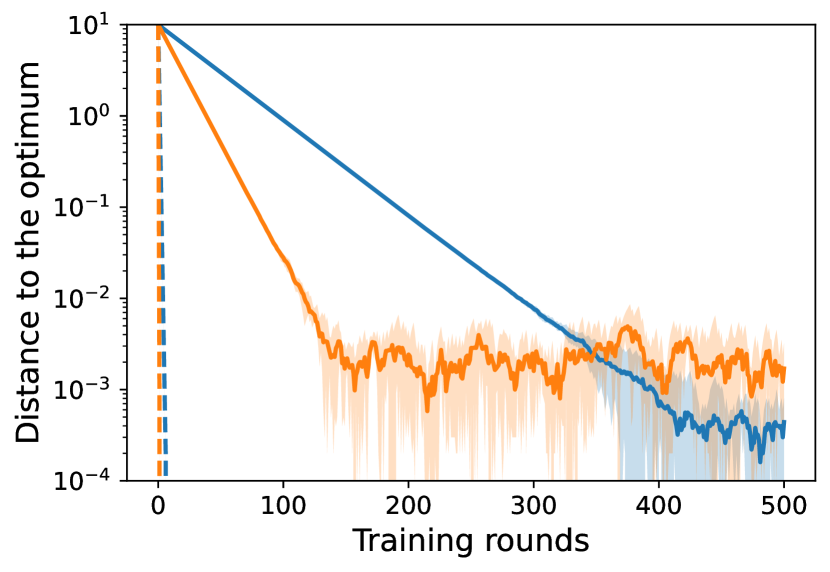
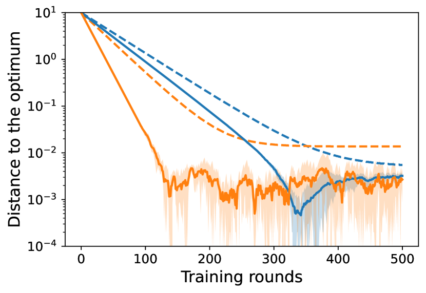
Figure 1: Simulations on quadratic functions. The left plot, middle plot, right plot are for Group 1, Group 2, Group 3 in Table 2 respectively. Shaded areas show the min-max values.

5 Experiments

In this section, we validate our theory empirically in two settings: (1) cross-silo settings with full client participation; (2) cross-device settings with partial client participation (Kairouz et al., 2021). We adopt the following models and datasets: (i) training LeNet-5 (LeCun et al., 1998) on the MNIST dataset (LeCun et al., 1998); (ii) training LeNet-5 on the FMNIST dataset (Xiao et al., 2017); (iii) training VGG-11 (Simonyan and Zisserman, 2014) on the CIFAR-10 dataset (Krizhevsky et al., 2009). We partition the training sets artificially with Extended Dirichlet strategy and spare the original test sets for computing test accuracy of the global model after each round.

Extended Dirichlet Strategy.

This is to generate arbitrarily heterogeneous data across clients by extending the popular Dirichlet-based data partition strategy (Yurochkin et al., 2019; Hsu et al., 2019). The difference is to add a step of allocating classes to determine the number of classes per client (denoted by $C$) before allocating samples via Dirichlet distribution (with concentrate parameter $\alpha$). Thus, the extended strategy can be denoted by $\text{Exdir}(C,\alpha)$. Suppose that there are $M$ clients. More details are deferred to Appendix F. The implementation is as follows:

• Allocating classes. Select $C$ classes for each client until each class is allocated to at least one client. Then we can obtain the prior distribution ${\bm{q}}_{c}\in\mathbb{R}^{M}$ over $M$ clients for any class $c$.

• Allocating samples. For any class $c$, we draw ${\bm{p}}_{c}\sim\text{Dir}(\alpha{\bm{q}}_{c})$ and then allocate a ${\bm{p}}_{c,m}$ proportion of the samples of class $c$ to client $m$. For example, ${\bm{q}}_{c}=[1,1,0,0,\ldots,]$ means that the samples of class $c$ are only allocated to the first 2 clients.

In this work, we use two partitions $\text{Exdir}(1,10.0)$ and $\text{Exdir}(2,10.0)$, where most clients own samples from one class in the former, and from two classes in the latter. So we call $\text{Exdir}(1,10.0)$ as extremely heterogeneous data and $\text{Exdir}(2,10.0)$ as moderately heterogeneous data. We note that the partition where clients owing samples from one class is not rare (Yu et al., 2020; Yang et al., 2021; Li et al., 2022). We note that the partition where clients owning samples from two classes is often seen as pathological (McMahan et al., 2017), so it needs more attention on how much data partitions can affect local objectives.

Cross-silo settings.

The training data is partitioned to 10 clients according to $\text{Exdir}(1,10.0)$ and $\text{Exdir}(2,10.0)$. Test accuracy results with varying local steps on CIFAR-10 are shown in Figure 2. We have the following observations: (i) data heterogeneity hurts the performance of SSL. The accuracy curves on $\text{Exdir}(1,10.0)$ exhibit unstable spikes and slower convergence rate than on $\text{Exdir}(2,10.0)$. This phenomenon is more obvious on curves with a large number of local steps. (ii) Increasing the number of local steps can help the convergence, yet excessive steps can even have negative impacts. From $K=5$ to $K=10$, the performance of SSL improves, yet from $K=10$ to $K=20$, $30$, it drops consistently. (iii) It can be seen that SSL outperforms FedAvg significantly on extremely heterogeneous data, yet slightly on moderately heterogeneous data. Interestingly, SSL shows more robust to the choice of $K$ in the extreme case than FedAvg while the opposite is true in the moderate case. From $K=5$ to $K=30$, the performance of FedAvg drops heavily in the left plot yet improves consistently in the right plot. These observations validate our theory.

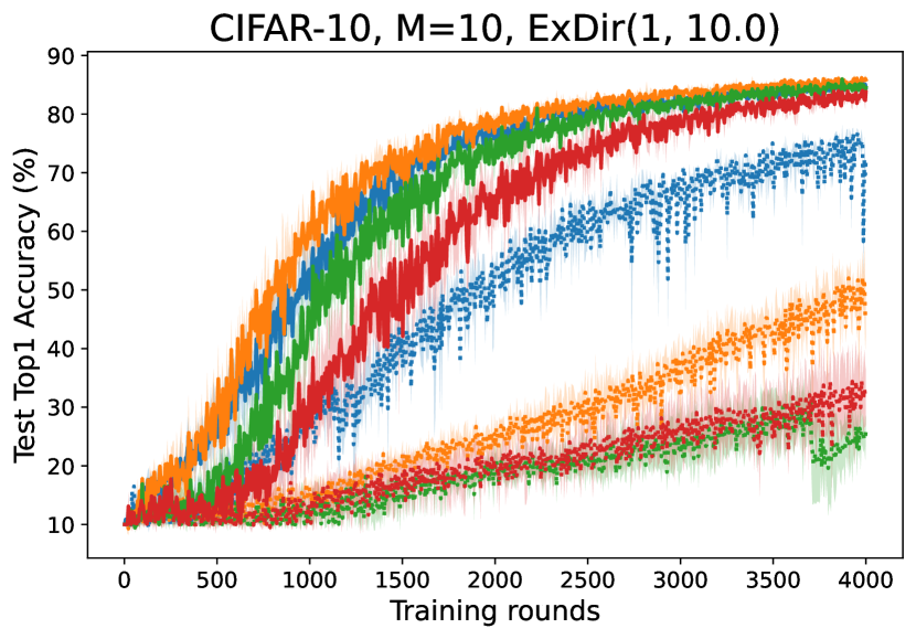
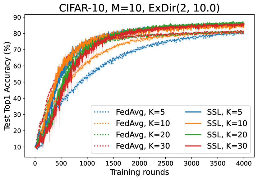
Figure 2: Test accuracy results with varying number of local steps on CIFAR-10 in cross-silo settings. The shaded areas show the standard deviation.

Cross-device settings.

We highlight the comparison in cross-device settings considering the practical scenario of SL (resource-constrained edge devices). The training data is partitioned to 500 clients according to $\text{Exdir}(1,10.0)$ and $\text{Exdir}(2,10.0)$ for all datasets MNIST, FMNIST and CIFAR-10. For FedAvg, 10 clients are selected in each round. SSL only runs for 1/10 number of the total rounds of FedAvg for fair comparisons. Note that we evaluate the performance of the global model after the training of every 10 clients, which is seen as one “training rounds” here. The results with varying local steps are reported in Table 3. It can be seen that (i) SSL outperforms FedAvg significantly in extremely heterogeneous data on cross-device settings (i.e., $\text{Exdir}(1,10.0)$). For CIFAR-10, the training of FedAvg almost dies when $K=10$, $20$. Even when $K$ is small, FedAvg struggle to converge. It is not surprising that FedAvg performs awfully in this extremely heterogeneous data. Because there may be only a subset of the total labels selected for training in each round, causing a large sample variance when partial clients are selected (see (12)). FedAvg shows better in cross-silo settings with the same local steps (left plot in Figure 2) validate it. In this case, client selection turns vital for FedAvg (Fraboni et al., 2021). The experiments in Li et al. (2022) can validate our results. These match our theory in Section 3.3. Besides, we find that (ii) SSL has no clear advantage on moderately heterogeneous data. On FMNIST, FedAvg even shows better than SSL and more local steps seem to enlarge the gap. In addition, the degradation of SSL on MNIST, FMNIST from $\text{Exdir}(1,10.0)$ to $\text{Exdir}(2,10.0)$ is because of the difference on the number of total training rounds. These match our analysis in Section 4.

Table 3: Test Accuracy results in cross-device settings. 1000 rounds are run for $\text{ExDir}(1,10.0)$ and 400 rounds for $\text{ExDir}(2,10.0)$ on MNIST, FMNIST. 4000 rounds are for both two partitions on CIFAR-10. Results are averaged across 3 random seeds and the last 20 rounds. The column 30% and 75% show the minimum number of rounds required to reach 30% and 75% accuracies.

Setup		$\text{ExDir}(1,10.0)$				$\text{ExDir}(2,10.0)$
		FedAvg		SSL		FedAvg		SSL
		ACC (%)	30%	ACC (%)	30%	ACC (%)	75%	ACC (%)	75%
CIFAR-10	$K=5$	$29.06\pm{\color[rgb]{.5,.5,.5}6.46}$	3666	$\textbf{81.34}\pm{\color[rgb]{.5,.5,.5}1.35}$	604	$75.92\pm{\color[rgb]{.5,.5,.5}1.17}$	3210	$\textbf{84.57}\pm{\color[rgb]{.5,.5,.5}0.90}$	1004
	$K=10$	$14.00\pm{\color[rgb]{.5,.5,.5}5.66}$	-	$\textbf{82.20}\pm{\color[rgb]{.5,.5,.5}1.33}$	483	$81.17\pm{\color[rgb]{.5,.5,.5}0.55}$	2153	$\textbf{82.95}\pm{\color[rgb]{.5,.5,.5}1.70}$	966
	$K=20$	$10.00\pm{\color[rgb]{.5,.5,.5}0.00}$	-	$\textbf{80.60}\pm{\color[rgb]{.5,.5,.5}1.62}$	673	$81.26\pm{\color[rgb]{.5,.5,.5}0.60}$	1614	$\textbf{85.24}\pm{\color[rgb]{.5,.5,.5}0.79}$	998
	$K=30$	-	-	-	-	$80.47\pm{\color[rgb]{.5,.5,.5}0.69}$	1618	$\textbf{84.52}\pm{\color[rgb]{.5,.5,.5}0.86}$	966
FMNIST	$K=10$	$39.90\pm{\color[rgb]{.5,.5,.5}6.08}$	492	$\textbf{80.38}\pm{\color[rgb]{.5,.5,.5}2.80}$	19	$\textbf{81.77}\pm{\color[rgb]{.5,.5,.5}1.15}$	127	$78.25\pm{\color[rgb]{.5,.5,.5}2.28}$	162
	$K=20$	$38.78\pm{\color[rgb]{.5,.5,.5}6.51}$	490	$\textbf{76.39}\pm{\color[rgb]{.5,.5,.5}3.15}$	25	$\textbf{83.55}\pm{\color[rgb]{.5,.5,.5}1.13}$	87	$76.58\pm{\color[rgb]{.5,.5,.5}3.18}$	103
MNIST	$K=10$	$56.43\pm{\color[rgb]{.5,.5,.5}11.54}$	274	$\textbf{98.84}\pm{\color[rgb]{.5,.5,.5}0.19}$	16	$98.15\pm{\color[rgb]{.5,.5,.5}0.13}$	25	$98.57\pm{\color[rgb]{.5,.5,.5}0.36}$	10
	$K=20$	$51.86\pm{\color[rgb]{.5,.5,.5}10.66}$	274	$\textbf{98.85}\pm{\color[rgb]{.5,.5,.5}0.12}$	14	$98.35\pm{\color[rgb]{.5,.5,.5}0.14}$	18	$98.56\pm{\color[rgb]{.5,.5,.5}0.33}$	8

6 Conclusion

In this work, we have derived the convergence guarantee of SSL for strongly convex, general convex and non-convex objectives on heterogeneous data. In particular, we have compared SSL against FedAvg, showing that the guarantee of SSL is better than FedAvg on heterogeneous data. Experimental results show that SSL outperforms FedAvg on extremely heterogeneous data, especially in cross-device settings. We believe that this work can bridge the gap between FL and SL, provide deep understanding of both approaches and guide the application deployment in real world.

Appendix

  [sections] [sections]l1

 

Appendix A Notations and technical lemmas

A.1 Notations

Table 4 summarizes the notations appearing in this paper.

Table 4: Summary of key notations.

Symbol	Description
$R,r$	number, index of training rounds
$M,m$	number, index of clients
$K,k$	number, index of local update steps
$\pi$	$\{\pi_{1},\pi_{2},\ldots,\pi_{M}\}$ is a permutation of $\{1,2,\ldots,M\}$
$S$	number of clients selected for training per round with partial client participation
$\eta$	learning rate (or stepsize)
$\tilde{\eta}$	effective learning rate ($\tilde{\eta}\coloneqq MK\eta$ in SSL and $\tilde{\eta}\coloneqq K\eta$ in FedAvg)
$\mu$	$\mu$-strong convexity constant
$L$	$L$-smoothness constant (Asm. 1)
$\sigma$	upper bound on variance of stochastic gradients (Asm. 2 on stochasticity)
$B,\zeta$	constants in Asm. 3 to bound heterogeneity everywhere
$\zeta_{\ast}$	constants in Asm. 3 to bound heterogeneity at the optimum
$F/F_{m}$	global objective/local objective of client $m$
${\mathbf{x}}^{r}$	global model parameters in the $r$-th round
${\mathbf{x}}_{m}^{(r,k)}$	local model parameters    after the $k$-th local update with client $\pi_{m}$ in the $r$-th round
${\mathbf{g}}_{\pi_{m}}^{(r,k)}$	${\mathbf{g}}_{\pi_{m}}^{(r,k)}\coloneqq\nabla f_{\pi_{m}}({\mathbf{x}}_{m}^{(r,k)};\xi_{m})$ denotes the stochastic gradients of $F_{\pi_{m}}$    regarding model parameters ${\mathbf{x}}_{m}^{(r,k)}$, on the sample $\xi_{m}$
$\text{ExDir}(C,\alpha)$	Extended Dirichlet strategy with parameters $C$ and $\alpha$.    Decreasing the values of $C$, $\alpha$ results in higher data heterogeneity. (Sec. F.2).

A.2 Basic identities and inequalities

These identities and inequalities are mostly from Mishchenko et al. (2020); Karimireddy et al. (2020); Zhou (2018); Garrigos and Gower (2023).

For any random variable $X$, letting the variance can be decomposed as

$$\mathbb{E}{\left\lVert X-\mathbb{E}{X}\right\rVert^{2}}=\mathbb{E}{\left\lVert X\right\rVert^{2}}-\left\lVert\mathbb{E}{X}\right\rVert^{2}$$ (13)

For the discrete random variables, it holds that

$$\frac{1}{m}\sum_{i=1}^{m}{\left\lVert{\bm{x}}_{i}-\bar{{\bm{x}}}\right\rVert}^{2}=\frac{1}{m}\sum_{i=1}^{m}{\left\lVert{\bm{x}}_{i}\right\rVert}^{2}-{\left\lVert\frac{1}{m}\sum_{i=1}^{m}{\bm{x}}_{i}\right\rVert}^{2},$$ (14)

for given vectors ${\bm{x}}_{1},\ldots,{\bm{x}}_{m}\in\mathbb{R}^{d}$ and their average $\bar{{\bm{x}}}$.

Jensen’s inequality.

For any convex function $h$ and any vectors ${\bm{x}}_{1},\dotsc,{\bm{x}}_{m}$ we have

$$h\left(\frac{1}{m}\sum_{i=1}^{m}{\bm{x}}_{i}\right)\leq\frac{1}{m}\sum_{i=1}^{m}f({\bm{x}}_{i}).$$ (15)

As a special case with $f(x)=\left\lVert x\right\rVert^{2}$, we obtain

$${\left\lVert\frac{1}{m}\sum_{i=1}^{m}{\bm{x}}_{i}\right\rVert}^{2}\leq\frac{1}{m}\sum_{i=1}^{m}\left\lVert{\bm{x}}_{i}\right\rVert^{2}.$$ (16)

Smoothness and (general) convexity, strong convexity.

There are some useful inequalities with respect to $L$-smoothness (Assumption 1), convexity and $\mu$-strong convexity. Their proofs can be found in Zhou (2018); Garrigos and Gower (2023).

Bregman Divergence associated with function $h$ and arbitrary ${\bm{x}}$, ${\bm{y}}$ is denoted as

$$D_{h}({\bm{x}},{\bm{y}})\coloneqq h({\bm{x}})-h({\bm{y}})-\left\langle\nabla h({\bm{y}}),{\bm{x}}-{\bm{y}}\right\rangle$$

When the function $h$ is convex, the divergence is strictly non-negative. A more formal definition can be found in Orabona (2019). One corollary (Chen and Teboulle, 1993) called three-point-identity is,

$$D_{h}({\bm{z}},{\bm{x}})+D_{h}({\bm{x}},{\bm{y}})-D_{h}({\bm{z}},{\bm{y}})=\left\langle\nabla h({\bm{y}})-\nabla h({\bm{x}}),{\bm{z}}-{\bm{x}}\right\rangle$$

where ${\bm{x}},{\bm{y}},{\bm{z}}$ is three points in the domain.

Let $h$ be $L$-smooth. With the definition of Bregman divergence, a useful consequence of $L$-smoothness is

$$D_{h}({\bm{x}},{\bm{y}})=h({\bm{x}})-h({\bm{y}})-\left\langle\nabla h({\bm{y}}),{\bm{x}}-{\bm{y}}\right\rangle\leq\frac{L}{2}\left\lVert{\bm{x}}-{\bm{y}}\right\rVert^{2}$$ (17)

Further, If $h$ is $L$-smooth and lower bounded by $h_{\ast}$, then

$${\left\lVert\nabla h({\bm{x}})\right\rVert}^{2}\leq 2L\left(h({\bm{x}})-h_{\ast}\right).$$ (18)

Then if $h$ is $L$-smooth and convex (The definition of convexity can be found in Boyd et al. (2004)), it holds that

$$D_{h}({\bm{x}},{\bm{y}})\geq\frac{1}{2L}\left\lVert\nabla h({\bm{x}})-\nabla h({\bm{y}})\right\rVert^{2}.$$ (19)

The function $h:\mathbb{R}^{d}\to\mathbb{R}$ is $\mu$-strongly convex if and only if there exists a convex function $g:\mathbb{R}^{d}\to\mathbb{R}$ such that $h({\bm{x}})=g({\bm{x}})+\frac{\mu}{2}\left\lVert{\bm{x}}\right\rVert^{2}$.

If $h$ is $\mu$-strongly convexity, it holds that

$$\frac{\mu}{2}\left\lVert{\bm{x}}-{\bm{y}}\right\rVert^{2}\leq D_{h}({\bm{x}},{\bm{y}})$$ (20)

A.3 Technical lemmas

Lemma 1 (Wang et al. (2020)).

Suppose $\{A_{k}\}_{k=1}^{T}$ is a sequence of random matrices and $\mathbb{E}[A_{k}|A_{k-1},A_{k-2},\dots,A_{1}]=\bm{0},\forall k$. Then,

$$\mathbb{E}\left[\left\lVert\sum_{k=1}^{T}A_{k}\right\rVert_{\tiny{\mbox{F}}}^{2}\right]=\sum_{k=1}^{T}\mathbb{E}\left[\left\lVert A_{k}\right\rVert_{\tiny{\mbox{F}}}^{2}\right].$$

Proof.

This is the Lemma 2 of Wang et al. (2020). Similar conclusions can be also found in Stich and Karimireddy (2019); Karimireddy et al. (2020). ∎

Lemma 2 (Karimireddy et al. (2020)).

The following holds for any $L$-smooth and $\mu$-strongly convex function $h$, and any ${\bm{x}},{\bm{y}},{\bm{z}}$ in the domain of $h$:

$$\left\langle\nabla h({\bm{x}}),{\bm{z}}-{\bm{y}}\right\rangle\geq h({\bm{z}})-h({\mathbf{y}})+\frac{\mu}{4}\left\lVert{\bm{y}}-{\bm{z}}\right\rVert^{2}-L\left\lVert{\bm{z}}-{\bm{x}}\right\rVert^{2}.$$ (21)

Proof.

This is Lemma 5 (perturbed strong convexity) in Karimireddy et al. (2020). ∎

Lemma 3 (Simple Random Sampling).

Let $X_{1},X_{2},\ldots,X_{M}\in\mathbb{R}^{d}$ be fixed units. The population mean and population variance are give as

$$\textstyle\overline{X}\coloneqq\frac{1}{M}\sum_{i=1}^{M}X_{i} \textstyle\sigma^{2}\coloneqq\frac{1}{M}\sum_{i=1}^{M}\left\lVert X_{i}-\overline{X}\right\rVert^{2}.$$

Sample $S\in[M]=\{1,2,\ldots,M\}$ units ${\mathbf{x}}_{\pi_{1}},{\mathbf{x}}_{\pi_{2}},\ldots{\mathbf{x}}_{\pi_{S}}$ from the population. There are two possible ways of simple random sampling, well known as “sampling with replacement” and “sampling without replacement”. For these two ways, the expectation and variance of the sample mean $\overline{\mathbf{x}}_{\pi}\coloneqq\frac{1}{S}\sum_{s=1}^{S}{\mathbf{x}}_{\pi_{s}}$ satisfies

• Sampling without replacement (SWOR).

  $$\mathbb{E}[\overline{\mathbf{x}}_{\pi}]=\overline{X} \mathbb{E}\left[\left\lVert\overline{\mathbf{x}}_{\pi}-\overline{X}\right\rVert^{2}\right]=\frac{M-S}{S(M-1)}\sigma^{2}$$ (22)

• Sampling with replacement (SWR).

  $$\mathbb{E}[\overline{\mathbf{x}}_{\pi}]=\overline{X} \mathbb{E}\left[\left\lVert\overline{\mathbf{x}}_{\pi}-\overline{X}\right\rVert^{2}\right]=\frac{\sigma^{2}}{S}$$ (23)

Proof.

This lemma is mainly based on the Lemma 1 in Mishchenko et al. (2020) and Appendix G Extension: Incorporating Client Sampling in Wang et al. (2020).

Expectation of the sample mean

• (SWOR) Note $\Pr({\mathbf{x}}_{\pi_{s}}=X_{i})=\frac{1}{M}$ since every unit has the same probability to be selected.

  $$\mathbb{E}[\overline{\mathbf{x}}_{\pi}]=\mathbb{E}\left[\frac{1}{S}\sum_{s=1}^{S}{\mathbf{x}}_{s}\right]=\frac{1}{S}\sum_{s=1}^{S}\mathbb{E}\left[{\mathbf{x}}_{s}\right]=\frac{1}{S}\sum_{s=1}^{S}\left[\sum_{i=1}^{M}\Pr({\mathbf{x}}_{s}=X_{i})X_{i}\right]=\frac{1}{S}\sum_{s=1}^{S}\left[\frac{1}{M}\sum_{i=1}^{M}X_{i}\right]=\overline{X}$$

• (SWR) $\mathbb{E}[\overline{\mathbf{x}}_{\pi}]=\overline{X}$, same as SRSWOR, since $\Pr({\mathbf{x}}_{\pi_{s}}=X_{i})=\frac{1}{M}$.

Variance of the sample mean

$$\mathbb{E}\left\lVert\overline{\mathbf{x}}_{\pi}-\overline{X}\right\rVert^{2} =\mathbb{E}\left\lVert\frac{1}{S}\sum_{s=1}^{S}{\mathbf{x}}_{\pi_{s}}-\overline{X}\right\rVert^{2}=\mathbb{E}\left\lVert\frac{1}{S}\sum_{s=1}^{S}({\mathbf{x}}_{\pi_{s}}-\overline{X})\right\rVert^{2}=\frac{1}{S^{2}}\mathbb{E}\left\lVert\sum_{s=1}^{S}({\mathbf{x}}_{\pi_{s}}-\overline{X})\right\rVert^{2}$$

$$=\frac{1}{S^{2}}\sum_{s=1}^{S}\mathrm{Var}({\mathbf{x}}_{\pi_{s}})+\frac{1}{S^{2}}\sum_{s=1}^{S}\sum_{t=1,t\neq s}^{S}\mathrm{Cov}({\mathbf{x}}_{\pi_{s}},{\mathbf{x}}_{\pi_{t}})$$

Since $\mathrm{Var}({\mathbf{x}}_{\pi_{s}})=\mathbb{E}\left\lVert{\mathbf{x}}_{\pi_{s}}-\mathbb{E}[{\mathbf{x}}_{\pi_{s}}]\right\rVert^{2}=\mathbb{E}\left\lVert{\mathbf{x}}_{\pi_{s}}-\overline{X}\right\rVert^{2}$, we have

$$\frac{1}{S^{2}}\sum_{s=1}^{S}\mathrm{Var}({\mathbf{x}}_{\pi_{s}})=\frac{1}{S^{2}}\sum_{s=1}^{S}\left[\sum_{i=1}^{M}\Pr({\mathbf{x}}_{\pi_{s}}=X_{i})(X_{i}-\overline{X})^{2}\right]=\frac{1}{S^{2}}\sum_{s=1}^{S}\left[\frac{1}{M}\sum_{i=1}^{M}(X_{i}-\overline{X})^{2}\right]=\frac{\sigma^{2}}{S}$$

For the covariance term, we need to consider two cases:

• (SWOR) For $s\neq t$, we have

  $$\mathrm{Cov}({\mathbf{x}}_{\pi_{s}},{\mathbf{x}}_{\pi_{t}})=\mathbb{E}\left\langle{\mathbf{x}}_{\pi_{s}}-\overline{X},{\mathbf{x}}_{\pi_{t}}-\overline{X}\right\rangle=\sum_{i=1}^{M}\sum_{j=1,j\neq i}^{M}\left[\Pr({\mathbf{x}}_{\pi_{s}}=X_{i},{\mathbf{x}}_{\pi_{t}}=X_{j})\left\langle X_{i}-\overline{X},X_{j}-\overline{X}\right\rangle\right],$$

  Since there are $M(M-1)$ possible combinations of $({\mathbf{x}}_{\pi_{s}},{\mathbf{x}}_{\pi_{t}})$, and each has the same probability, we get $\Pr({\mathbf{x}}_{\pi_{s}}=X_{i},{\mathbf{x}}_{\pi_{t}}=X_{j})=\frac{1}{M(M-1)}$. As a consequence, we have

  $$\mathrm{Cov}({\mathbf{x}}_{\pi_{s}},{\mathbf{x}}_{\pi_{t}}) =\frac{1}{M(M-1)}\sum_{i=1}^{M}\sum_{j=1,j\neq i}^{M}\left[\left\langle X_{i}-\overline{X},X_{j}-\overline{X}\right\rangle\right]$$

  $$=\frac{1}{M(M-1)}\sum_{i=1}^{M}\sum_{j=1}^{M}\left[\left\langle X_{i}-\overline{X},X_{j}-\overline{X}\right\rangle\right]-\frac{1}{M(M-1)}\sum_{i=1}^{M}\left\lVert X_{i}-\overline{X}\right\rVert^{2}$$

  $$=\frac{1}{M(M-1)}\sum_{i=1}^{M}\left[\left\langle X_{i}-\overline{X},\underbrace{\sum_{j=1}^{M}(X_{j}-\overline{X})}_{=0}\right\rangle\right]-\frac{1}{M(M-1)}\sum_{i=1}^{M}\left\lVert X_{i}-\overline{X}\right\rVert^{2}$$

  $$=-\frac{\sigma^{2}}{M-1}$$ (24)

  Thus we have

  $$\mathbb{E}\left\lVert\overline{\mathbf{x}}_{\pi}-\overline{X}\right\rVert^{2}=\frac{\sigma^{2}}{S}-\frac{S(S-1)}{S^{2}}\left(\frac{\sigma^{2}}{M-1}\right)=\frac{(M-S)\sigma^{2}}{S(M-1)}$$

• (SWR) For $s\neq t$, we have $\mathrm{Cov}({\mathbf{x}}_{\pi_{s}},{\mathbf{x}}_{\pi_{t}})=0$ since $x_{s}$ and $x_{t}$ are independent. Thus we get

  $$\mathbb{E}\left\lVert\overline{\mathbf{x}}_{\pi}-\overline{X}\right\rVert^{2}=\frac{\sigma^{2}}{S}$$

Now, we complete the proof. When $M$ is infinite (or large enough), we get $\frac{(\mathbb{E}\left\lVert\overline{\mathbf{x}}_{\pi}-\overline{X}\right\rVert^{2})_{\textrm{SWOR}}}{(\mathbb{E}\left\lVert\overline{\mathbf{x}}_{\pi}-\overline{X}\right\rVert^{2})_{\textrm{SWR}}}\approx 1-\frac{S}{M}$. This constant has appeared in Lemma 7 (one round progress) in Karimireddy et al. (2020) and Section 7 (Using a Subset of Machines in Each Round) in Woodworth et al. (2020). ∎

Appendix B Proofs of Theorem 1

In this section, we provide the proof of Theorem 1 for the strongly convex, general convex and non-convex cases in B.2, B.3 and B.4, respectively.

B.1 Additional technical lemmas

Lemma 4.

Under the same conditions of Lemma 3, use the way “sampling without replacement” and let $\mathcal{K}(i)\coloneqq\begin{cases}K-1,\;1\leq i\leq m-1\\ k-1,\;i=m\end{cases}$ ($k$, $m$ are not constants). It holds that

$$\sum_{m=1}^{M}\sum_{k=0}^{K-1}\mathbb{E}\left\lVert\sum_{i=1}^{m}\sum_{j=0}^{{\mathcal{K}}(i)}\left({\mathbf{x}}_{\pi_{i}}-\overline{X}\right)\right\rVert^{2}\leq\frac{1}{3}M^{2}K^{3}\sigma^{2}$$ (25)

Proof.

Let us focus on the term in the following:

$$\mathbb{E}\left\lVert\sum_{i=1}^{m}\sum_{j=0}^{{\mathcal{K}}(i)}\left({\mathbf{x}}_{\pi_{i}}-\overline{X}\right)\right\rVert^{2}=\mathbb{E}\left\lVert K\sum_{i=1}^{m-1}\left({\mathbf{x}}_{\pi_{i}}-\overline{X}\right)+k\left({\mathbf{x}}_{\pi_{m}}-\overline{X}\right)\right\rVert^{2}$$

$$=\mathbb{E}\left\lVert K\sum_{i=1}^{m-1}\left({\mathbf{x}}_{\pi_{i}}-\overline{X}\right)\right\rVert^{2}+\mathbb{E}\left\lVert k\left({\mathbf{x}}_{\pi_{m}}-\overline{X}\right)\right\rVert^{2}+2\mathbb{E}\left\langle K\sum_{i=1}^{m-1}\left({\mathbf{x}}_{\pi_{i}}-\overline{X}\right),k\left({\mathbf{x}}_{\pi_{m}}-\overline{X}\right)\right\rangle$$ (26)

For the first term on the right hand side in (26), using (22), we have

$$\mathbb{E}\left\lVert K\sum_{i=1}^{m-1}\left({\mathbf{x}}_{\pi_{i}}-\overline{X}\right)\right\rVert^{2}=\frac{(m-1)(M-(m-1))}{M-1}K^{2}\sigma^{2}$$

For the second term on the right hand side in (26), we have

$$\mathbb{E}\left\lVert k\left({\mathbf{x}}_{\pi_{m}}-\overline{X}\right)\right\rVert^{2}=k^{2}\mathbb{E}\left\lVert{\mathbf{x}}_{\pi_{m}}-\overline{X}\right\rVert^{2}=k^{2}\sigma^{2}$$

For the third term on the right hand side in (26), we have

$$2\mathbb{E}\left\langle K\sum_{i=1}^{m-1}\left({\mathbf{x}}_{\pi_{i}}-\overline{X}\right),k\left({\mathbf{x}}_{\pi_{m}}-\overline{X}\right)\right\rangle =2Kk\sum_{i=1}^{m-1}\mathbb{E}\left\langle{\mathbf{x}}_{\pi_{i}}-\overline{X},{\mathbf{x}}_{\pi_{m}}-\overline{X}\right\rangle$$

$$=2Kk(m-1)\left(-\frac{\sigma^{2}}{M-1}\right)=\frac{2(m-1)}{M-1}Kk\sigma^{2},$$

where we use (24) in the last equality, since $i\in\{1,2,\ldots,m-1\}\neq m$. Combining these three preceding equations, we get

$$\mathbb{E}\left\lVert\sum_{i=1}^{m}\sum_{j=0}^{{\mathcal{K}}(i)}\left({\mathbf{x}}_{\pi_{i}}-\overline{X}\right)\right\rVert^{2}=\frac{(m-1)(M-(m-1))}{M-1}K^{2}\sigma^{2}+k^{2}\sigma^{2}-\frac{2(m-1)}{M-1}Kk\sigma^{2}$$ (27)

Then summing over $m$ and $k$, we can get

$$\sum_{m=1}^{M}\sum_{k=0}^{K-1}\mathbb{E}\left\lVert\sum_{i=1}^{m}\sum_{j=0}^{{\mathcal{K}}(i)}\left({\mathbf{x}}_{\pi_{i}}-\overline{X}\right)\right\rVert^{2} =K^{3}\sigma^{2}\left(\frac{M}{M-1}\sum_{m=1}^{M}(m-1)-\frac{1}{M-1}\sum_{m=1}^{M}(m-1)^{2}\right)$$

$$\quad+M\sigma^{2}\sum_{k=0}^{K-1}k^{2}+\frac{2K\sigma^{2}}{M-1}\sum_{m=1}^{M}(m-1)\sum_{k=0}^{K-1}k$$ (28)

Then applying the fact that $\sum_{k=1}^{K-1}k=\frac{(K-1)K}{2}$ and $\sum_{k=1}^{K-1}k^{2}=\frac{(K-1)K(2K-1)}{6}$, we can simplify the preceding equation as

$$\sum_{m=1}^{M}\sum_{k=0}^{K-1}\mathbb{E}\left\lVert\sum_{i=1}^{m}\sum_{j=0}^{{\mathcal{K}}(i)}\left({\mathbf{x}}_{\pi_{i}}-\overline{X}\right)\right\rVert^{2}=\frac{1}{6}(M^{2}K^{3}+MK)\sigma^{2}\leq\frac{1}{3}M^{2}K^{3}\sigma^{2},$$ (29)

which is the claim of this lemma. ∎

B.2 Strongly convex case

B.2.1 Finding the recursion

Lemma 5.

Let Assumptions 1, 2, (5) of 3 hold and assume that all the local objectives are $\mu$-strongly convex. If the learning rate satisfies $\eta\leq\frac{1}{6LMK}$, then it holds that

$$\mathbb{E}\left\lVert{\mathbf{x}}^{r+1}-{\mathbf{x}}^{\ast}\right\rVert^{2} \leq\left(1-\tfrac{\mu MK\eta}{2}\right)\left\lVert{\mathbf{x}}^{r}-{\mathbf{x}}^{*}\right\rVert^{2}-MK\eta(2-6LMK\eta)\mathbb{E}D_{F}({\mathbf{x}}^{r},{\mathbf{x}}^{\ast})+3MK\eta^{2}\sigma^{2}$$

$$\quad+L\eta(2+3LMK\eta)\sum_{m=1}^{M}\sum_{k=0}^{K-1}\mathbb{E}\left\lVert{\mathbf{x}}_{m}^{(r,k)}-{\mathbf{x}}^{r}\right\rVert^{2}$$ (30)

Proof.

Without otherwise stated, the expectation is conditioned on ${\mathbf{x}}^{r}$. The update rule of SL in round $r$ can be written as $\displaystyle{\mathbf{x}}^{r+1}={\mathbf{x}}^{r}-\eta\sum_{m=1}^{M}\sum_{k=0}^{K-1}{\mathbf{g}}_{\pi_{m}}^{(r,k)}$, where ${\mathbf{g}}_{\pi_{m}}^{(r,k)}=\nabla f_{\pi_{m}}({\mathbf{x}}_{m}^{(r,k)};\xi_{m}^{(r,k)})$. As a consequence, we can get,

$$\mathbb{E}\left\lVert{\mathbf{x}}^{r+1}-{\mathbf{x}}^{\ast}\right\rVert^{2}=\left\lVert{\mathbf{x}}^{r}-{\mathbf{x}}^{*}\right\rVert^{2}-2\eta\sum_{m=1}^{M}\sum_{k=0}^{K-1}\left\langle\nabla F_{\pi_{m}}({\mathbf{x}}_{m}^{(r,k)}),{\mathbf{x}}^{r}-{\mathbf{x}}^{\ast}\right\rangle+\eta^{2}\mathbb{E}\left\lVert\sum_{m=1}^{M}\sum_{k=0}^{K-1}{\mathbf{g}}_{\pi_{m}}^{(r,k)}\right\rVert^{2}$$ (31)

Using Lemma 2 with ${\bm{x}}={\mathbf{x}}_{m}^{(r,k)}$, ${\bm{y}}={\mathbf{x}}^{\ast}$, ${\bm{z}}={\mathbf{x}}^{r}$ and $h=F_{\pi_{m}}$, we have

$$-2\eta\sum_{m=1}^{M}\sum_{k=0}^{K-1}\mathbb{E}\left\langle\nabla F_{\pi_{m}}({\mathbf{x}}_{m}^{(r,k)}),{\mathbf{x}}^{r}-{\mathbf{x}}^{\ast}\right\rangle$$

$$\leq-2\eta\sum_{m=1}^{M}\sum_{k=0}^{K-1}\mathbb{E}\left[F_{\pi_{m}}({\mathbf{x}}^{r})-F_{\pi_{m}}({\mathbf{x}}^{\ast})+\frac{\mu}{4}\left\lVert{\mathbf{x}}^{r}-{\mathbf{x}}^{\ast}\right\rVert^{2}-L\left\lVert{\mathbf{x}}_{m}^{(r,k)}-{\mathbf{x}}^{r}\right\rVert^{2}\right]$$

$$\leq-2MK\eta\left(F({\mathbf{x}}^{r})-F({\mathbf{x}}^{\ast})\right)-\frac{\mu MK\eta}{2}\left\lVert{\mathbf{x}}^{r}-{\mathbf{x}}^{\ast}\right\rVert^{2}+2L\eta\sum_{m=1}^{M}\sum_{k=0}^{K-1}\mathbb{E}\left\lVert{\mathbf{x}}_{m}^{(r,k)}-{\mathbf{x}}^{r}\right\rVert^{2}$$ (32)

For the third term on the right hand side in (31), using Jensen’s inequality, we have:

$$\mathbb{E}\left\lVert\sum_{m=1}^{M}\sum_{k=0}^{K-1}{\mathbf{g}}_{\pi_{m}}^{(r,k)}\right\rVert^{2} \leq 3\mathbb{E}\left\lVert\sum_{m=1}^{M}\sum_{k=0}^{K-1}{\mathbf{g}}_{\pi_{m}}^{(r,k)}-\sum_{m=1}^{M}\sum_{k=0}^{K-1}\nabla F_{\pi_{m}}({\mathbf{x}}_{m}^{(r,k)})\right\rVert^{2}$$

$$+3\mathbb{E}\left\lVert\sum_{m=1}^{M}\sum_{k=0}^{K-1}\nabla F_{\pi_{m}}({\mathbf{x}}_{m}^{(r,k)})-\sum_{m=1}^{M}\sum_{k=0}^{K-1}\nabla F_{\pi_{m}}({\mathbf{x}}^{r})\right\rVert^{2}+3\mathbb{E}\left\lVert\sum_{m=1}^{M}\sum_{k=0}^{K-1}\nabla F_{\pi_{m}}({\mathbf{x}}^{r})\right\rVert^{2}$$ (33)

For the first term on the right hand side in (33), using Lemma 1, we have

$$\mathbb{E}\left\lVert\sum_{m=1}^{M}\sum_{k=0}^{K-1}{\mathbf{g}}_{\pi_{m}}^{(r,k)}-\sum_{m=1}^{M}\sum_{k=0}^{K-1}\nabla F_{\pi_{m}}({\mathbf{x}}_{m}^{(r,k)})\right\rVert^{2}\leq\sum_{m=1}^{M}\sum_{k=0}^{K-1}\mathbb{E}\left\lVert{\mathbf{g}}_{\pi_{m}}^{(r,k)}-\nabla F_{\pi_{m}}({\mathbf{x}}_{m}^{(r,k)})\right\rVert^{2}\leq MK\sigma^{2}$$ (34)

For the second term on the right hand side in (33), we have

$$\mathbb{E}\left\lVert\sum_{m=1}^{M}\sum_{k=0}^{K-1}\nabla F_{\pi_{m}}({\mathbf{x}}_{m}^{(r,k)})-\sum_{m=1}^{M}\sum_{k=0}^{K-1}\nabla F_{\pi_{m}}({\mathbf{x}}^{r})\right\rVert^{2} \leq MK\sum_{m=1}^{M}\sum_{k=0}^{K-1}\mathbb{E}\left\lVert\nabla F_{\pi_{m}}({\mathbf{x}}_{m}^{(r,k)})-\nabla F_{\pi_{m}}({\mathbf{x}}^{r})\right\rVert^{2}$$

$$\overset{\text{Asm.}~{}\ref{asm:L-smoothness}}{\leq}L^{2}MK\sum_{m=1}^{M}\sum_{k=0}^{K-1}\mathbb{E}\left\lVert{\mathbf{x}}_{m}^{(r,k)}-{\mathbf{x}}^{r}\right\rVert^{2}$$ (35)

For the third term on the right hand side in (33), we have

$$\mathbb{E}\left\lVert\sum_{m=1}^{M}\sum_{k=0}^{K-1}\nabla F_{\pi_{m}}({\mathbf{x}}^{r})\right\rVert^{2}\leq M^{2}K^{2}\mathbb{E}\left\lVert\nabla F({\mathbf{x}}^{r})\right\rVert^{2}\overset{\eqref{eq:L-smoothness grad bound}}{\leq}2LM^{2}K^{2}D_{F}({\mathbf{x}}^{r},{\mathbf{x}}^{\ast})$$ (36)

As a result, the third term on the right hand side in (31) can be bounded as:

$$\mathbb{E}\left\lVert\sum_{m=1}^{M}\sum_{k=0}^{K-1}{\mathbf{g}}_{\pi_{m}}^{(r,k)}\right\rVert^{2} \leq 3L^{2}MK\sum_{m=1}^{M}\sum_{k=0}^{K-1}\mathbb{E}\left\lVert{\mathbf{x}}_{m}^{(r,k)}-{\mathbf{x}}^{r}\right\rVert^{2}+6LM^{2}K^{2}D_{F}({\mathbf{x}}^{r},{\mathbf{x}}^{\ast})+3MK\sigma^{2}$$ (37)

Then substituting (32) and (37) into (31), we have

$$\mathbb{E}\left\lVert{\mathbf{x}}^{r+1}-{\mathbf{x}}^{\ast}\right\rVert^{2} \leq\left(1-\tfrac{\mu MK\eta}{2}\right)\left\lVert{\mathbf{x}}^{r}-{\mathbf{x}}^{*}\right\rVert^{2}-MK\eta(2-6LMK\eta)D_{F}({\mathbf{x}}^{r},{\mathbf{x}}^{\ast})+3MK\eta^{2}\sigma^{2}$$

$$\quad+L\eta(2+3LMK\eta)\sum_{m=1}^{M}\sum_{k=0}^{K-1}\mathbb{E}\left\lVert{\mathbf{x}}_{m}^{(r,k)}-{\mathbf{x}}^{r}\right\rVert^{2}$$ (38)

The claim of this lemma follows after taking unconditional expectation. ∎

B.2.2 Bounding the client drift with (5)

Similar to the client drift in FL (Karimireddy et al., 2020), we define the client drift in SSL as $\displaystyle E_{r}\coloneqq\sum_{m=1}^{M}\sum_{k=0}^{K-1}\mathbb{E}\left\lVert{\mathbf{x}}_{m}^{(r,k)}-{\mathbf{x}}^{r}\right\rVert^{2}$.

Lemma 6.

For any learning rate satisfying $\eta\leq\frac{1}{6LMK}$, the client drift caused by local updates is bounded, as given by:

$$\mathbb{E}\left[E_{r}\right] \leq\frac{9}{2}LM^{3}K^{3}\eta^{2}\mathbb{E}\left[D_{F}({\mathbf{x}}^{r},{\mathbf{x}}^{\ast})\right]+\frac{9}{4}M^{2}K^{2}\eta^{2}\sigma^{2}+\frac{3}{2}M^{2}K^{3}\eta^{2}\zeta_{\ast}^{2}$$ (39)

Proof.

Without otherwise stated, the expectation is conditioned on ${\mathbf{x}}^{r}$. Beginning with $\mathbb{E}\left\lVert{\mathbf{x}}_{m}^{(r,k)}-{\mathbf{x}}^{r}\right\rVert^{2}$. Considering

$${\mathbf{x}}_{m}^{(r,k)}-{\mathbf{x}}^{r}={\mathbf{x}}_{m}^{(r,k)}-{\mathbf{x}}_{m}^{(r,0)}+{\mathbf{x}}_{m}^{(r,0)}-{\mathbf{x}}_{m-1}^{(r,0)}+\cdots+{\mathbf{x}}_{2}^{(r,0)}-{\mathbf{x}}_{1}^{(r,0)}=-\eta\sum_{i=1}^{m}\sum_{j=0}^{{\mathcal{K}}(i)}{\mathbf{g}}_{\pi_{i}}^{(r,j)},$$ (40)

with $\mathcal{K}(i)\coloneqq\begin{cases}K-1,\;1\leq i\leq m-1\\ k-1,\;i=m\end{cases},$ we have

$$\mathbb{E}\left\lVert{\mathbf{x}}_{m}^{(r,k)}-{\mathbf{x}}^{r}\right\rVert^{2} =\eta^{2}\mathbb{E}\left\lVert\sum_{i=1}^{m}\sum_{j=0}^{{\mathcal{K}}(i)}{\mathbf{g}}_{\pi_{i}}^{(r,j)}\right\rVert^{2}$$ (41)

Then using the Jensen’s inequality to the preceding equation, we have

$$\mathbb{E}\left\lVert{\mathbf{x}}_{m}^{(r,k)}-{\mathbf{x}}^{r}\right\rVert^{2}$$

$$\leq 4\eta^{2}\mathbb{E}\left\lVert\sum_{i=1}^{m}\sum_{j=0}^{{\mathcal{K}}(i)}{\mathbf{g}}_{\pi_{i}}^{(r,j)}-\sum_{i=1}^{m}\sum_{j=0}^{{\mathcal{K}}(i)}\nabla F_{\pi_{i}}({\mathbf{x}}_{i}^{(r,j)})\right\rVert^{2}+4\eta^{2}\mathbb{E}\left\lVert\sum_{i=1}^{m}\sum_{j=0}^{{\mathcal{K}}(i)}\nabla F_{\pi_{i}}({\mathbf{x}}_{i}^{(r,j)})-\sum_{i=1}^{m}\sum_{j=0}^{{\mathcal{K}}(i)}\nabla F_{\pi_{i}}({\mathbf{x}}^{r})\right\rVert^{2}$$

$$\quad+4\eta^{2}\mathbb{E}\left\lVert\sum_{i=1}^{m}\sum_{j=0}^{{\mathcal{K}}(i)}\nabla F_{\pi_{i}}({\mathbf{x}}^{r})-\sum_{i=1}^{m}\sum_{j=0}^{{\mathcal{K}}(i)}\nabla F_{\pi_{i}}({\mathbf{x}}^{\ast})\right\rVert^{2}+4\eta^{2}\mathbb{E}\left\lVert\sum_{i=1}^{m}\sum_{j=0}^{{\mathcal{K}}(i)}\nabla F_{\pi_{i}}({\mathbf{x}}^{\ast})\right\rVert^{2}$$ (42)

Applying Lemma 1 to the first term and Jensen’s inequality to the last three terms on the right hand side in (42) respectively, we get

$$\mathbb{E}\left\lVert{\mathbf{x}}_{m}^{(r,k)}-{\mathbf{x}}^{r}\right\rVert^{2} \leq 4\eta^{2}\sum_{i=1}^{m}\sum_{j=0}^{{\mathcal{K}}(i)}\mathbb{E}\left\lVert{\mathbf{g}}_{\pi_{i}}^{(r,j)}-\nabla F_{\pi_{i}}({\mathbf{x}}_{i}^{(r,j)})\right\rVert^{2}+4\eta^{2}{\mathcal{K}}\sum_{i=1}^{m}\sum_{j=0}^{{\mathcal{K}}(i)}\mathbb{E}\left\lVert\nabla F_{\pi_{i}}({\mathbf{x}}_{i}^{(r,j)})-\nabla F_{\pi_{i}}({\mathbf{x}}^{r})\right\rVert^{2}$$

$$\;+4\eta^{2}{\mathcal{K}}\sum_{i=1}^{m}\sum_{j=0}^{{\mathcal{K}}(i)}\mathbb{E}\left\lVert\nabla F_{\pi_{i}}({\mathbf{x}}^{r})-\nabla F_{\pi_{i}}({\mathbf{x}}^{\ast})\right\rVert^{2}+4\eta^{2}\mathbb{E}\left\lVert\sum_{i=1}^{m}\sum_{j=0}^{{\mathcal{K}}(i)}\nabla F_{\pi_{i}}({\mathbf{x}}^{\ast})\right\rVert^{2},$$ (43)

where $\displaystyle{\mathcal{K}}\coloneqq\sum_{i=1}^{m}\sum_{j=0}^{{\mathcal{K}}(i)}1=(m-1)K+k$. For the first term on the right hand side in (43), we have

$$\mathbb{E}\left\lVert{\mathbf{g}}_{\pi_{i}}^{(r,j)}-\nabla F_{\pi_{i}}({\mathbf{x}}_{i}^{(r,j)})\right\rVert^{2}\overset{\eqref{eq:asm:stochasticity}}{\leq}\sigma^{2}$$

For the second term on the right hand side in (43), we have

$$\mathbb{E}\left\lVert\nabla F_{\pi_{i}}({\mathbf{x}}_{m}^{(r,j)})-\nabla F_{\pi_{i}}({\mathbf{x}}^{r})\right\rVert^{2}\overset{\text{Asm.}~{}\ref{asm:L-smoothness}}{\leq}L^{2}\mathbb{E}\left\lVert{\mathbf{x}}_{i}^{(r,j)}-{\mathbf{x}}^{r}\right\rVert^{2}$$

For the third term on the right hand side in (43), we have

$$\mathbb{E}\left\lVert\nabla F_{\pi_{i}}({\mathbf{x}}^{r})-\nabla F_{\pi_{i}}({\mathbf{x}}^{\ast})\right\rVert^{2}\overset{\eqref{eq:bregman lower smooth}}{\leq}2LD_{F_{\pi_{i}}}({\mathbf{x}}^{r},{\mathbf{x}}^{\ast})$$ (44)

As a result, we can get

$$\mathbb{E}\left\lVert{\mathbf{x}}_{m}^{(r,k)}-{\mathbf{x}}^{r}\right\rVert^{2} \leq 4L^{2}\eta^{2}{\mathcal{K}}\sum_{i=1}^{m}\sum_{j=0}^{{\mathcal{K}}(i)}\mathbb{E}\left\lVert{\mathbf{x}}_{i}^{(r,j)}-x^{r}\right\rVert^{2}+8L\eta^{2}{\mathcal{K}}\sum_{i=1}^{m}\sum_{j=0}^{{\mathcal{K}}(i)}D_{F_{\pi_{i}}}({\mathbf{x}}^{r},{\mathbf{x}}^{\ast})$$

$$\quad+4{\mathcal{K}}\eta^{2}\sigma^{2}+4\eta^{2}\mathbb{E}\left\lVert\sum_{i=1}^{m}\sum_{j=0}^{{\mathcal{K}}(i)}\nabla F_{\pi_{i}}({\mathbf{x}}^{\ast})\right\rVert^{2}$$ (45)

Returning to $\displaystyle E_{r}\coloneqq\sum_{m=1}^{M}\sum_{k=0}^{K-1}\mathbb{E}\left\lVert{\mathbf{x}}_{m}^{(r,k)}-{\mathbf{x}}^{r}\right\rVert^{2}$, we have

$$E_{r} \leq 4L^{2}\eta^{2}\sum_{m=1}^{M}\sum_{k=0}^{K-1}{\mathcal{K}}\sum_{i=1}^{M}\sum_{j=0}^{K-1}\mathbb{E}\left\lVert{\mathbf{x}}_{i}^{(r,j)}-x^{r}\right\rVert^{2}+8L\eta^{2}\sum_{m=1}^{M}\sum_{k=0}^{K-1}{\mathcal{K}}\sum_{i=1}^{M}\sum_{j=0}^{K-1}D_{F_{\pi_{i}}}({\mathbf{x}}^{r},{\mathbf{x}}^{\ast})$$

$$\quad+4\sum_{m=1}^{M}\sum_{k=0}^{K-1}{\mathcal{K}}\eta^{2}\sigma^{2}+4\eta^{2}\sum_{m=1}^{M}\sum_{k=0}^{K-1}\mathbb{E}\left\lVert\sum_{i=1}^{m}\sum_{j=0}^{{\mathcal{K}}(i)}\nabla F_{\pi_{i}}({\mathbf{x}}^{\ast})\right\rVert^{2}$$ (46)

Then using

$$\sum_{m=1}^{M}\sum_{k=0}^{K-1}{\mathcal{K}}=\sum_{m=1}^{M}(m-1)K^{2}+\sum_{m=1}^{M}\sum_{k=0}^{K-1}k=\frac{1}{2}M(M-1)K^{2}+\frac{1}{2}MK(K-1)\leq\frac{1}{2}M^{2}K^{2}$$

and

$$\sum_{m=1}^{M}\sum_{k=0}^{K-1}\mathbb{E}\left\lVert\sum_{i=1}^{m}\sum_{j=0}^{{\mathcal{K}}(i)}\nabla F_{\pi_{i}}({\mathbf{x}}^{\ast})\right\rVert^{2}\overset{\eqref{eq:asm:heterogeneity:optimum}}{\leq}\frac{1}{3}M^{2}K^{3}\zeta_{\ast}^{2}$$

where we use Lemma 4 with ${\mathbf{x}}_{\pi_{i}}=\nabla F_{\pi_{i}}({\mathbf{x}}^{\ast})$ and $\overline{X}=\frac{1}{M}\sum_{m=1}^{M}F_{\pi_{i}}({\mathbf{x}}^{\ast})=F({\mathbf{x}}^{\ast})=0$, we have

$$\mathbb{E}\left[E_{r}\right] \leq 2L^{2}M^{2}K^{2}\eta^{2}\mathbb{E}\left[E_{r}\right]+4LM^{3}K^{3}\eta^{2}D_{F}({\mathbf{x}}^{r},{\mathbf{x}}^{\ast})+2M^{2}K^{2}\eta^{2}\sigma^{2}+\frac{4}{3}M^{2}K^{3}\eta^{2}\zeta_{\ast}^{2}$$ (47)

After rearranging the preceding inequality, we get

$$(1-2L^{2}M^{2}K^{2}\eta^{2})\mathbb{E}\left[E_{r}\right]\leq 4LM^{3}K^{3}\eta^{2}D_{F}({\mathbf{x}}^{r},{\mathbf{x}}^{\ast})+2M^{2}K^{2}\eta^{2}\sigma^{2}+\frac{4}{3}M^{2}K^{3}\eta^{2}\zeta_{\ast}^{2}$$ (48)

Finally, using the choice of $\eta$, $LMK\eta\leq\frac{1}{6}$, which implies $1-2L^{2}M^{2}K^{2}\eta^{2}\geq\frac{8}{9}$, we have

$$\mathbb{E}\left[E_{r}\right] \leq\frac{9}{2}LM^{3}K^{3}\eta^{2}D_{F}({\mathbf{x}}^{r},{\mathbf{x}}^{\ast})+\frac{9}{4}M^{2}K^{2}\eta^{2}\sigma^{2}+\frac{3}{2}M^{2}K^{3}\eta^{2}\zeta_{\ast}^{2}.$$ (49)

The claim of this lemma follows after taking unconditional expectations. ∎

B.2.3 Tuning the learning rate

Here we make a clear version of Lemma 1 in Karimireddy et al. (2020) based on the works Stich (2019a); Stich and Karimireddy (2019).

Lemma 7 (Karimireddy et al. (2020)).

Two non-negative sequences $\{r_{t}\}_{t\geq 0}$, $\{s_{t}\}_{t\geq 0}$, which satisfies the relation

$$r_{t+1}\leq(1-a\gamma_{t})r_{t}-b\gamma_{t}s_{t}+c\gamma_{t}^{2},$$ (50)

for all $t\geq 0$ and for parameters $b>0$, $a,c\geq 0$ and non-negative learning rates $\{\gamma_{t}\}_{t\geq 0}$ with $\gamma_{t}\leq\frac{1}{d}$, $\forall t\geq 0$, for a parameter $d\geq a$, $d>0$.

Selection of weights for average. Then there exists a constant learning rate $\gamma_{t}=\gamma\leq\frac{1}{d}$ and the weights $w_{t}:=(1-a\gamma)^{-(t+1)}$ and $W_{T}:=\sum_{t=0}^{T}w_{t}$, making it hold that:

$$\Psi_{T}=\frac{b}{W_{T}}\sum_{t=0}^{T}s_{t}w_{t}\leq 3ar_{0}(1-a\gamma)^{(T+1)}+c\gamma\leq 3ar_{0}\exp\left[-a\gamma(T+1)\right]+c\gamma.$$ (51)

Tuning the learning rate carefully. By tuning the learning rate in (51), for $(T+1)\geq\frac{1}{2a\gamma}$, we have

$$\Psi_{T}=\tilde{\mathcal{O}}\left(ar_{0}\exp\left[-\frac{aT}{d}\right]+\frac{c}{aT}\right).$$ (52)

Proof.

We start by rearranging (50) and multiplying both sides with $w_{t}$:

$$bs_{t}w_{t}\leq\frac{w_{t}(1-a\gamma)r_{t}}{\gamma}-\frac{w_{t}r_{t+1}}{\gamma}+c\gamma w_{t}=\frac{w_{t-1}r_{t}}{\gamma}-\frac{w_{t}r_{t+1}}{\gamma}+c\gamma w_{t}\,.$$

By summing from $t=0$ to $t=T$, we obtain a telescoping sum:

$$\frac{b}{W_{T}}\sum_{t=0}^{T}s_{t}w_{t}\leq\frac{1}{\gamma W_{T}}\left(w_{0}(1-a\gamma)r_{0}-w_{T}r_{T+1}\right)+c\gamma\,,$$

and hence

$$\Psi_{T}=\frac{b}{W_{T}}\sum_{t=0}^{T}s_{t}w_{t}\leq\frac{b}{W_{T}}\sum_{t=0}^{T}s_{t}w_{t}+\frac{w_{T}r_{T+1}}{\gamma W_{T}}\leq\frac{r_{0}}{\gamma W_{T}}+c\gamma$$ (53)

Note that in the proof of Lemma 2 in Stich (2019a), they use $W_{T}\geq w_{T}=(1-a\gamma)^{-(T+1)}$ to estimate $W_{T}$. It is reasonable given that $w_{T}$ is extremely larger than all the terms $w_{t}$ ($t<T$) when $T$ is large. Yet Karimireddy et al. (2020) goes further, showing that $W_{T}$ can be estimated more precisely:

$$W_{T}=\sum_{0}^{T}w_{t}=(1-a\gamma)^{-(T+1)}\sum_{t=0}^{T}(1-a\gamma)^{t}=(1-a\gamma)^{-(T+1)}\left(\frac{1-(1-a\gamma)^{T+1}}{a\gamma}\right)$$

When $(T+1)\geq\frac{1}{2a\gamma}$, $(1-a\gamma)^{T+1}\leq\exp(-a\gamma(T+1))\leq e^{-\frac{1}{2}}\leq\frac{2}{3}$, so it follows that

$$W_{T}=(1-a\gamma)^{-(T+1)}\left(\frac{1-(1-a\gamma)^{T+1}}{a\gamma}\right)\geq\frac{(1-a\gamma)^{-(T+1)}}{3a\gamma}$$

With the estimates

• $W_{T}=(1-a\gamma)^{-(T+1)}\sum_{t=0}^{T}(1-a\gamma)^{t}\leq\frac{w_{T}}{a\gamma}$ (here we leverage $a\gamma\leq\frac{a}{d}\leq 1$),

• and $W_{T}\geq\frac{(1-a\gamma)^{-(T+1)}}{3a\gamma}$,

we can further simplified the terms on both sides in (53):

$$\Psi_{T}\leq 3ar_{0}(1-a\gamma)^{(T+1)}+c\gamma\leq 3ar_{0}\exp\left[-a\gamma(T+1)\right]+c\gamma$$

which is the first result of this lemma.

Now the lemma follows by carefully tuning $\gamma$ in (51). Consider the two cases:

• If $\frac{1}{d}>\frac{\ln(\max\{2,a^{2}r_{0}T/c\})}{aT}$ then we choose $\gamma=\frac{\ln(\max\{2,a^{2}r_{0}T/c\})}{aT}$ and get that

  $$\tilde{\mathcal{O}}\left(3ar_{0}\exp[-\ln(\max\{2,a^{2}r_{0}T/c\})]\right)+\tilde{\mathcal{O}}\left(\frac{c}{aT}\right)=\tilde{\mathcal{O}}\left(\frac{c}{aT}\right)\,,$$

  as in case $2\geq a^{2}r_{0}T/c$ it holds $ar_{0}\leq\frac{2c}{aT}$.

• If otherwise $\frac{1}{2a(T+1)}\leq\frac{1}{d}\leq\frac{\ln(\max\{2,a^{2}r_{0}T/c\})}{aT}$ (Note $\frac{1}{2a(T+1)}\leq\frac{\ln(2)}{aT}\leq\frac{\ln(\max\{2,a^{2}r_{0}T/c\})}{aT}$) then we pick $\gamma=\frac{1}{d}$ and get that

  $$3ar_{0}\exp\left[-\frac{aT}{d}\right]+\frac{c}{d}\leq 3ar_{0}\exp\left[-\frac{aT}{d}\right]+\frac{c\ln(\max\{2,a^{2}r_{0}T/c\})}{aT}=\tilde{\mathcal{O}}\left(ar_{0}\exp\left[-\frac{aT}{d}\right]+\frac{c}{aT}\right)$$

Combining these two cases, we get

$$\Psi_{T}=\tilde{\mathcal{O}}\left(ar_{0}\exp\left[-\frac{aT}{d}\right]+\frac{c}{aT}\right)$$

Note that this lemma holds when $(T+1)\geq\frac{1}{2a\gamma}$, so it restricts the value of $T$ (Lemma 2 in Stich (2019a) without this constraint). ∎

B.2.4 Proof of strongly convex case of Theorem 1 and Corollary 1

Proof of strongly convex case of Theorem 1.

Substituting (39) into (30) and using $LK\eta\leq\frac{1}{6}$, we can simplify the recursion as,

$$\mathbb{E}\left\lVert{\mathbf{x}}^{r+1}-{\mathbf{x}}^{*}\right\rVert^{2} \leq\left(1-\tfrac{\mu MK\eta}{2}\right)\mathbb{E}\left\lVert{\mathbf{x}}^{r}-{\mathbf{x}}^{\ast}\right\rVert^{2}-\frac{1}{2}MK\eta\mathbb{E}\left[D_{F}({\mathbf{x}}^{r},{\mathbf{x}}^{\ast})\right]+3MK\eta^{2}\sigma^{2}$$

$$\quad+\frac{45}{8}LM^{2}K^{2}\eta^{3}\sigma^{2}+\frac{15}{4}LM^{2}K^{3}\eta^{3}\zeta_{\ast}^{2}$$ (54)

Let $\tilde{\eta}=MK\eta$, we have

$$\mathbb{E}\left\lVert{\mathbf{x}}^{r+1}-{\mathbf{x}}^{*}\right\rVert^{2}\leq\left(1-\frac{\mu\tilde{\eta}}{2}\right)\mathbb{E}\left\lVert{\mathbf{x}}^{r}-{\mathbf{x}}^{\ast}\right\rVert^{2}-\frac{\tilde{\eta}}{2}\mathbb{E}\left[D_{F}({\mathbf{x}}^{r},{\mathbf{x}}^{\ast})\right]+\frac{3\tilde{\eta}^{2}\sigma^{2}}{MK}+\frac{45L\tilde{\eta}^{3}\sigma^{2}}{8MK}+\frac{15L\tilde{\eta}^{3}\zeta_{\ast}^{2}}{4M}$$ (55)

Applying Lemma 7 with $t=r$ ($T=R$), $\gamma=\tilde{\eta}$, $r_{t}=\mathbb{E}\left\lVert{\mathbf{x}}^{r}-{\mathbf{x}}^{*}\right\rVert^{2}$, $a=\frac{\mu}{2}$, $b=\frac{1}{2}$, $s_{t}=\mathbb{E}\left[D_{F}({\mathbf{x}}^{r},{\mathbf{x}}^{\ast})\right]=\mathbb{E}\left[F({\mathbf{x}}^{r})-F({\mathbf{x}}^{*})\right]$, $w_{t}=(1-a\tilde{\eta})^{-(r+1)}$, $c_{1}=\frac{3\sigma^{2}}{MK}$, $c_{2}=\frac{45L\sigma^{2}}{8MK}+\frac{15L\zeta_{\ast}^{2}}{4M}$ and $\frac{1}{d}=\frac{1}{6L}$ ($\tilde{\eta}=MK\eta\leq\frac{1}{6L}$).

Note that in Lemma 7, there are no terms containing $\gamma^{3}$. As the terms containing $\gamma^{3}$ is not the determining factor for the convergence rate, Lemma 7 can also be applied to this case (Karimireddy et al., 2020; Koloskova et al., 2020).

$$F(\bar{\mathbf{x}}^{R})-F({\mathbf{x}}^{\ast})\leq 3\mu\left\lVert{\mathbf{x}}^{0}-{\mathbf{x}}^{*}\right\rVert^{2}\exp\left[-\frac{1}{2}\mu\tilde{\eta}(R+1)\right]+\frac{6\tilde{\eta}\sigma^{2}}{MK}+\frac{45L\tilde{\eta}^{2}\sigma^{2}}{4MK}+\frac{15L\tilde{\eta}^{2}\zeta_{\ast}^{2}}{2M}$$ (56)

where $\bar{\mathbf{x}}^{R}=\frac{1}{W_{R}}\sum_{r=0}^{R}w_{r}{\mathbf{x}}^{r}$. Here we have $F(\bar{\mathbf{x}}^{R})-F({\mathbf{x}}^{\ast})\leq\frac{1}{W_{R}}\sum_{r=0}^{R}w_{r}\mathbb{E}\left[F({\mathbf{x}}^{r})-F({\mathbf{x}}^{*})\right]$, where the convexity of $F$ and Jensen’s inequality are used.

By tuning the learning rate carefully, we get

$$F(\bar{\mathbf{x}}^{R})-F({\mathbf{x}}^{\ast})=\tilde{\mathcal{O}}\left(\mu D^{2}\exp\left(-\frac{\mu}{12L}R\right)+\frac{\sigma^{2}}{\mu MKR}+\frac{L\sigma^{2}}{\mu^{2}MKR^{2}}+\frac{L\zeta_{\ast}^{2}}{\mu^{2}MR^{2}}\right)$$ (57)

with $D=\left\lVert{\mathbf{x}}^{0}-{\mathbf{x}}^{\ast}\right\rVert$. ∎

B.3 General convex case

B.3.1 Tuning the learning rate

Lemma 8 (Koloskova et al. (2020)).

Two non-negative sequences $\{r_{t}\}_{t\geq 0}$, $\{s_{t}\}_{t\geq 0}$, which satisfies the relation

$$r_{t+1}\leq r_{t}-b\gamma_{t}s_{t}+c_{1}\gamma_{t}^{2}+c_{2}\gamma_{t}^{3}$$

for all $t\geq 0$ and for parameters $b>0$, $c_{1},c_{2}\geq 0$ and non-negative learning rates $\{\gamma_{t}\}_{t\geq 0}$ with $\gamma_{t}\leq\frac{1}{d}$, $\forall t\geq 0$, for a parameter $d>0$.

Selection of weights for average. Then there exists a constant learning rate $\gamma=\gamma_{t}\leq\frac{1}{d}$ and the weights $w_{t}=1$ and $W_{T}=\sum_{t=0}^{T}w_{t}$, making it hod that:

$$\Psi_{T}\coloneqq\frac{b}{T+1}\sum_{t=0}^{T}s_{t}\leq\frac{r_{0}}{\gamma(T+1)}+c_{1}\gamma+c_{2}\gamma^{2}$$ (58)

Tuning the learning rate carefully. By tuning the learning rate carefully in (58), we have

$$\Psi_{T}\leq 2c_{1}^{\frac{1}{2}}\left(\frac{r_{0}}{T+1}\right)^{\frac{1}{2}}+2c_{2}^{\frac{1}{3}}\left(\frac{r_{0}}{T+1}\right)^{\frac{2}{3}}+\frac{dr_{0}}{T+1}.$$ (59)

Proof.

For constant learning rates $\gamma_{t}=\gamma$ we can derive the estimate

$$\Psi_{T}=\frac{1}{\gamma(T+1)}\sum_{t=0}^{T}\left(r_{t}-r_{t+1}\right)+c_{1}\gamma+c_{2}\gamma^{2}\leq\frac{r_{0}}{\gamma(T+1)}+c_{1}\gamma+c_{2}\gamma^{2},$$

which is the first result (58) of this lemma. Let $\frac{r_{0}}{\gamma(T+1)}=c_{1}\gamma$ and $\frac{r_{0}}{\gamma(T+1)}=c_{2}\gamma^{2}$, yielding two choices of $\gamma$, $\gamma=\left(\frac{r_{0}}{c_{1}(T+1)}\right)^{\frac{1}{2}}$ and $\gamma=\left(\frac{r_{0}}{c_{2}(T+1)}\right)^{\frac{1}{3}}$. Then choosing $\gamma=\min\left\{\left(\frac{r_{0}}{c_{1}(T+1)}\right)^{\frac{1}{2}},\left(\frac{r_{0}}{c_{2}(T+1)}\right)^{\frac{1}{3}},\frac{1}{d}\right\}\leq\frac{1}{d}$, there are three cases:

• If $\gamma=\frac{1}{d}$, which implies that $\gamma=\frac{1}{d}\leq\left(\frac{r_{0}}{c_{1}(T+1)}\right)^{\frac{1}{2}}$ and $\gamma=\frac{1}{d}\leq\left(\frac{r_{0}}{c_{2}(T+1)}\right)^{\frac{1}{3}}$, then

  $$\Psi_{T}\leq\frac{dr_{0}}{T+1}+\frac{c_{1}}{d}+\frac{c_{2}}{d^{2}}\leq\frac{dr_{0}}{T+1}+c_{1}^{\frac{1}{2}}\left(\frac{r_{0}}{T+1}\right)^{\frac{1}{2}}+c_{2}^{\frac{1}{3}}\left(\frac{r_{0}}{T+1}\right)^{\frac{2}{3}}$$

• If $\gamma=\left(\frac{r_{0}}{c_{1}(T+1)}\right)^{\frac{1}{2}}$, which implies that $\gamma=\left(\frac{r_{0}}{c_{1}(T+1)}\right)^{\frac{1}{2}}\leq\left(\frac{r_{0}}{c_{2}(T+1)}\right)^{\frac{1}{3}}$, then

  $$\Psi_{T}\leq 2c_{1}\left(\frac{r_{0}}{c_{1}(T+1)}\right)^{\frac{1}{2}}+c_{2}\left(\frac{r_{0}}{c_{1}(T+1)}\right)\leq 2c_{1}^{\frac{1}{2}}\left(\frac{r_{0}}{T+1}\right)^{\frac{1}{2}}+c_{2}^{\frac{1}{3}}\left(\frac{r_{0}}{T+1}\right)^{\frac{2}{3}}$$

• If $\gamma=\left(\frac{r_{0}}{c_{2}(T+1)}\right)^{\frac{1}{3}}$, which implies that $\gamma=\left(\frac{r_{0}}{c_{2}(T+1)}\right)^{\frac{1}{3}}\leq\left(\frac{r_{0}}{c_{1}(T+1)}\right)^{\frac{1}{2}}$, then

  $$\Psi_{T}\leq c_{1}\left(\frac{r_{0}}{c_{2}(T+1)}\right)^{\frac{1}{3}}+2c_{2}^{\frac{1}{3}}\left(\frac{r_{0}}{T+1}\right)^{\frac{2}{3}}\leq c_{1}^{\frac{1}{2}}\left(\frac{r_{0}}{T+1}\right)^{\frac{1}{2}}+2c_{2}^{\frac{1}{3}}\left(\frac{r_{0}}{T+1}\right)^{\frac{2}{3}}$$

Combining these three cases, we get the second result of this lemma. ∎

B.3.2 Proof of general convex case of Theorem 1 and Corollary 1

Proof of general convex case of Theorem 1.

Let $\mu=0$ in (55), we get the simplified recursion of general convex case,

$$\mathbb{E}\left\lVert{\mathbf{x}}^{r+1}-{\mathbf{x}}^{*}\right\rVert^{2}\leq\mathbb{E}\left\lVert{\mathbf{x}}^{r}-{\mathbf{x}}^{\ast}\right\rVert^{2}-\frac{\tilde{\eta}}{2}\mathbb{E}\left[D_{F}({\mathbf{x}}^{r},{\mathbf{x}}^{\ast})\right]+\frac{3\tilde{\eta}^{2}\sigma^{2}}{MK}+\frac{45L\tilde{\eta}^{3}\sigma^{2}}{8MK}+\frac{15L\tilde{\eta}^{3}\zeta_{\ast}^{2}}{4M}$$ (60)

Then Applying Lemma 8 with $t=r$ ($T=R$), $\gamma=\tilde{\eta}$, $r_{t}=\mathbb{E}\left\lVert{\mathbf{x}}^{r}-{\mathbf{x}}^{*}\right\rVert^{2}$, $b=\frac{1}{2}$, $s_{t}=\mathbb{E}\left[D_{F}({\mathbf{x}}^{r},{\mathbf{x}}^{\ast})\right]=\mathbb{E}\left[F({\mathbf{x}}^{r})-F({\mathbf{x}}^{*})\right]$, $w_{t}=1$, $c_{1}=\frac{3\sigma^{2}}{MK}$, $c_{2}=\frac{45L\sigma^{2}}{8MK}+\frac{15L\zeta_{\ast}^{2}}{4M}$ and $\frac{1}{d}=\frac{1}{6L}$ ($\tilde{\eta}=MK\eta\leq\frac{1}{6L}$), we can have

$$F(\bar{\mathbf{x}}^{R})-F({\mathbf{x}}^{\ast})\leq\frac{2\left\lVert{\mathbf{x}}^{0}-{\mathbf{x}}^{\ast}\right\rVert^{2}}{\tilde{\eta}R}+\frac{6\tilde{\eta}\sigma^{2}}{MK}+\frac{45L\tilde{\eta}^{2}\sigma^{2}}{4MK}+\frac{15L\tilde{\eta}^{2}\zeta_{\ast}^{2}}{2M},$$ (61)

where $\bar{\mathbf{x}}^{R}=\frac{1}{W_{R}}\sum_{r=0}^{R}w_{r}{\mathbf{x}}^{r}$. Here we have $F(\bar{\mathbf{x}}^{R})-F({\mathbf{x}}^{\ast})\leq\frac{1}{W_{R}}\sum_{r=0}^{R}w_{r}\mathbb{E}\left[F({\mathbf{x}}^{r})-F({\mathbf{x}}^{*})\right]$, with the convexity of $F$ and Jensen’s inequality. By tuning the learning rate carefully, we get

$$F(\bar{\mathbf{x}}^{R})-F({\mathbf{x}}^{\ast})={\mathcal{O}}\left(\frac{\sigma D}{\sqrt{MKR}}+\frac{\left(L\sigma^{2}D^{4}\right)^{1/3}}{(MK)^{1/3}R^{2/3}}+\frac{\left(L\zeta_{\ast}^{2}D^{4}\right)^{1/3}}{M^{1/3}R^{2/3}}+\frac{LD^{2}}{R}\right),$$ (62)

where $D=\left\lVert{\mathbf{x}}^{0}-{\mathbf{x}}^{\ast}\right\rVert$. ∎

B.4 Non-convex case

Lemma 9.

Under the same assumptions as Theorem 1, we can find the per-round recursion as

$$\mathbb{E}[F({\mathbf{x}}^{r+1})-F({\mathbf{x}}^{r})]\leq-\frac{MK\eta}{2}\left\lVert\nabla F({\mathbf{x}}^{r})\right\rVert^{2}+LMK\eta^{2}\sigma^{2}+\frac{L^{2}\eta}{2}\sum_{m=1}^{M}\sum_{k=0}^{K-1}\mathbb{E}\left\lVert{\mathbf{x}}_{m}^{(r,k)}-{\mathbf{x}}^{r}\right\rVert^{2}$$ (63)

Proof.

Without otherwise stated, the expectation is conditioned on ${\mathbf{x}}^{r}$. Beginning from $L$-smoothness,

$$D_{F}({\mathbf{x}}^{r+1},{\mathbf{x}}^{r})=F({\mathbf{x}}^{r+1})-F({\mathbf{x}}^{r})-\left\langle\nabla F({\mathbf{x}}^{r}),{\mathbf{x}}^{r+1}-{\mathbf{x}}^{r}\right\rangle\leq\frac{L}{2}\left\lVert{\mathbf{x}}^{r+1}-{\mathbf{x}}^{r}\right\rVert^{2},$$

and the update rule of SSL,

$${\mathbf{x}}^{r+1}={\mathbf{x}}^{r}-\eta\sum_{m=1}^{M}\sum_{k=0}^{K-1}{\mathbf{g}}_{\pi_{m}}^{(r,k)},$$

where ${\mathbf{g}}_{m}^{(r,k)}=\nabla f_{m}({\mathbf{x}}_{m}^{(r,k)};\xi_{m}^{(r,k)})$, we have

$$\mathbb{E}[F({\mathbf{x}}^{r+1})]-F({\mathbf{x}}^{r})\leq-M\eta\sum_{k=0}^{K-1}\mathbb{E}\left\langle\nabla F({\mathbf{x}}^{r}),\frac{1}{M}\sum_{m=1}^{M}\nabla F_{\pi_{m}}({\mathbf{x}}_{m}^{(r,k)})\right\rangle+\frac{L}{2}\mathbb{E}\left\lVert\frac{\eta}{M}\sum_{m=1}^{M}\sum_{k=0}^{K-1}{\mathbf{g}}_{\pi_{m}}^{r,k}\right\rVert^{2}$$ (64)

For the first term on the right hand side in (64), using $\left\langle a,b\right\rangle=\frac{1}{2}\left\lVert a\right\rVert^{2}+\frac{1}{2}\left\lVert b\right\rVert^{2}-\frac{1}{2}\left\lVert a-b\right\rVert^{2}$ with $a=\nabla F({\mathbf{x}}^{r})$ and $b=\frac{1}{M}\sum_{m=1}^{M}\nabla F_{\pi_{m}}({\mathbf{x}}_{m}^{(r,k)})$, we have

$$-M\eta\sum_{k=0}^{K-1}\mathbb{E}\left\langle\nabla F({\mathbf{x}}^{r}),\frac{1}{M}\sum_{m=1}^{M}\nabla F_{\pi_{m}}({\mathbf{x}}_{m}^{(r,k)})\right\rangle$$

$$\leq-\frac{M\eta}{2}\sum_{k=0}^{K-1}\mathbb{E}\left[\left\lVert\nabla F({\mathbf{x}}^{r})\right\rVert^{2}+\left\lVert\frac{1}{M}\sum_{m=1}^{M}\nabla F_{\pi_{m}}({\mathbf{x}}_{m}^{(r,k)})\right\rVert^{2}-\left\lVert\frac{1}{M}\sum_{m=1}^{M}\nabla F_{\pi_{m}}({\mathbf{x}}_{m}^{(r,k)})-\nabla F({\mathbf{x}}^{r})\right\rVert^{2}\right]$$

$$\overset{\eqref{eq:jensen norm},\text{Asm.~{}}\ref{asm:L-smoothness}}{\leq}-\frac{MK\eta}{2}\left\lVert\nabla F({\mathbf{x}}^{r})\right\rVert^{2}-\frac{M\eta}{2}\sum_{k=0}^{K-1}\mathbb{E}\left\lVert\frac{1}{M}\sum_{m=1}^{M}\nabla F_{\pi_{m}}({\mathbf{x}}_{m}^{(r,k)})\right\rVert^{2}+\frac{L^{2}\eta}{2}\sum_{m=1}^{M}\sum_{k=0}^{K-1}\mathbb{E}\left\lVert{\mathbf{x}}_{m}^{(r,k)}-{\mathbf{x}}^{r}\right\rVert^{2}$$ (65)

For the second term on the right hand side in (64), we have

$$\frac{L}{2}\mathbb{E}\left\lVert\eta\sum_{m=1}^{M}\sum_{k=0}^{K-1}{\mathbf{g}}_{\pi_{m}}^{r,k}\right\rVert^{2} \leq L\eta^{2}\mathbb{E}\left\lVert\sum_{m=1}^{M}\sum_{k=0}^{K-1}{\mathbf{g}}_{\pi_{m}}^{r,k}-\sum_{m=1}^{M}\sum_{k=0}^{K-1}\nabla F_{\pi_{m}}({\mathbf{x}}_{m}^{(r,k)})\right\rVert^{2}+L\eta^{2}\mathbb{E}\left\lVert\sum_{m=1}^{M}\sum_{k=0}^{K-1}\nabla F_{\pi_{m}}({\mathbf{x}}_{m}^{(r,k)})\right\rVert^{2}$$

$$\leq LMK\eta^{2}\sigma^{2}+L\eta^{2}\mathbb{E}\left\lVert\sum_{m=1}^{M}\sum_{k=0}^{K-1}\nabla F_{\pi_{m}}({\mathbf{x}}_{m}^{(r,k)})\right\rVert^{2}$$ (66)

Substituting (65) and (66) into (64), we have

$$\mathbb{E}[F({\mathbf{x}}^{r+1})]-F({\mathbf{x}}^{r}) \overset{\eqref{eq:jensen norm}}{\leq}-\frac{MK\eta}{2}\left\lVert\nabla F({\mathbf{x}}^{r})\right\rVert^{2}+\frac{L^{2}\eta}{2}\sum_{m=1}^{M}\sum_{k=0}^{K-1}\mathbb{E}\left\lVert{\mathbf{x}}_{m}^{(r,k)}-{\mathbf{x}}^{r}\right\rVert^{2}+LMK\eta^{2}\sigma^{2}$$

$$\quad-\frac{\eta}{2}(1-2LMK\eta)\frac{1}{M}\sum_{m=1}^{M}\sum_{k=0}^{K-1}\left\lVert\nabla F_{\pi_{m}}({\mathbf{x}}_{m}^{(r,k)})\right\rVert^{2}$$ (67)

Considering $MK\eta\leq\frac{1}{6L}$, the last term on the right hand side in the preceding inequality is negative. As a consequence, we have

$$\mathbb{E}[F({\mathbf{x}}^{r+1})]-F({\mathbf{x}}^{r}) \overset{\eqref{eq:jensen norm}}{\leq}-\frac{MK\eta}{2}\left\lVert\nabla F({\mathbf{x}}^{r})\right\rVert^{2}+LMK\eta^{2}\sigma^{2}+\frac{L^{2}\eta}{2}\sum_{m=1}^{M}\sum_{k=0}^{K-1}\mathbb{E}\left\lVert{\mathbf{x}}_{m}^{(r,k)}-{\mathbf{x}}^{r}\right\rVert^{2}$$

The claim follows after taking unconditional expectation. ∎

B.4.1 Bounding the client drift with (4)

Lemma 10.

Under the same assumptions as Theorem 2, for any learning rate satisfying $\eta\leq\frac{1}{6LK}$, the client drift $E_{r}$, defined as

$$E_{r}\coloneqq\sum_{m=1}^{M}\sum_{k=0}^{K-1}\mathbb{E}\left\lVert{\mathbf{x}}_{m}^{(r,k)}-{\mathbf{x}}^{r}\right\rVert^{2},$$

is bounded, as given by:

$$\mathbb{E}\left[E_{r}\right] \leq\frac{3}{2}M^{3}K^{3}\eta^{2}\mathbb{E}\left\lVert\nabla F({\mathbf{x}}^{r})\right\rVert^{2}+\frac{3}{2}M^{2}K^{3}B^{2}\eta^{2}\mathbb{E}\left\lVert\nabla F({\mathbf{x}}^{r})\right\rVert^{2}+\frac{9}{4}M^{2}K^{2}\eta^{2}\sigma^{2}+\frac{3}{2}M^{2}K^{3}\eta^{2}\zeta^{2}$$ (68)

Proof.

Without otherwise stated, the expectation is conditioned on ${\mathbf{x}}^{r}$. Beginning with $\mathbb{E}\left\lVert{\mathbf{x}}_{m}^{(r,k)}-{\mathbf{x}}^{r}\right\rVert^{2}$. Considering

$${\mathbf{x}}_{m}^{(r,k)}-{\mathbf{x}}^{r}={\mathbf{x}}_{m}^{(r,k)}-{\mathbf{x}}_{m}^{(r,0)}+{\mathbf{x}}_{m}^{(r,0)}-{\mathbf{x}}_{m-1}^{(r,0)}+\cdots+{\mathbf{x}}_{2}^{(r,0)}-{\mathbf{x}}_{1}^{(r,0)}=-\eta\sum_{i=1}^{m}\sum_{j=0}^{{\mathcal{K}}(i)}{\mathbf{g}}_{\pi_{i}}^{(r,j)},$$ (69)

with $\mathcal{K}(i)\coloneqq\begin{cases}K-1,\;1\leq i\leq m-1\\ k-1,\;i=m\end{cases},$ we have

$$\mathbb{E}\left\lVert{\mathbf{x}}_{m}^{(r,k)}-{\mathbf{x}}^{r}\right\rVert^{2} =\eta^{2}\mathbb{E}\left\lVert\sum_{i=1}^{m}\sum_{j=0}^{{\mathcal{K}}(i)}{\mathbf{g}}_{\pi_{i}}^{(r,j)}\right\rVert^{2}$$ (70)

Then using the Jensen’s inequality to the preceding equation, we have

$$\mathbb{E}\left\lVert{\mathbf{x}}_{m}^{(r,k)}-{\mathbf{x}}^{r}\right\rVert^{2}$$

$$\leq 4\eta^{2}\mathbb{E}\left\lVert\sum_{i=1}^{m}\sum_{j=0}^{{\mathcal{K}}(i)}{\mathbf{g}}_{\pi_{i}}^{(r,j)}-\sum_{i=1}^{m}\sum_{j=0}^{{\mathcal{K}}(i)}\nabla F_{\pi_{i}}({\mathbf{x}}_{i}^{(r,j)})\right\rVert^{2}+4\eta^{2}\mathbb{E}\left\lVert\sum_{i=1}^{m}\sum_{j=0}^{{\mathcal{K}}(i)}\nabla F_{\pi_{i}}({\mathbf{x}}_{i}^{(r,j)})-\sum_{i=1}^{m}\sum_{j=0}^{{\mathcal{K}}(i)}\nabla F_{\pi_{i}}({\mathbf{x}}^{r})\right\rVert^{2}$$

$$\quad+4\eta^{2}\mathbb{E}\left\lVert\sum_{i=1}^{m}\sum_{j=0}^{{\mathcal{K}}(i)}\nabla F_{\pi_{i}}({\mathbf{x}}^{r})-\sum_{i=1}^{m}\sum_{j=0}^{{\mathcal{K}}(i)}\nabla F({\mathbf{x}}^{r})\right\rVert^{2}+4\eta^{2}\mathbb{E}\left\lVert\sum_{i=1}^{m}\sum_{j=0}^{{\mathcal{K}}(i)}\nabla F({\mathbf{x}}^{r})\right\rVert^{2}$$ (71)

Applying Lemma 1 to the first term and Jensen’s inequality to the last three terms on the right hand side in (71) respectively, we get

$$\mathbb{E}\left\lVert{\mathbf{x}}_{m}^{(r,k)}-{\mathbf{x}}^{r}\right\rVert^{2} \leq 4\eta^{2}\sum_{i=1}^{m}\sum_{j=0}^{{\mathcal{K}}(i)}\mathbb{E}\left\lVert{\mathbf{g}}_{\pi_{i}}^{(r,j)}-\nabla F_{\pi_{i}}({\mathbf{x}}_{i}^{(r,j)})\right\rVert^{2}+4\eta^{2}{\mathcal{K}}\sum_{i=1}^{m}\sum_{j=0}^{{\mathcal{K}}(i)}\mathbb{E}\left\lVert\nabla F_{\pi_{i}}({\mathbf{x}}_{i}^{(r,j)})-\nabla F_{\pi_{i}}({\mathbf{x}}^{r})\right\rVert^{2}$$

$$+4\eta^{2}{\mathcal{A}}+4\eta^{2}{\mathcal{K}}^{2}\mathbb{E}\left\lVert\nabla F({\mathbf{x}}^{r})\right\rVert^{2}$$ (72)

where $\displaystyle{\mathcal{A}}=\mathbb{E}\left\lVert\sum_{i=1}^{m}\sum_{j=0}^{{\mathcal{K}}(i)}\nabla F_{\pi_{i}}({\mathbf{x}}^{r})-\sum_{i=1}^{m}\sum_{j=0}^{{\mathcal{K}}(i)}\nabla F({\mathbf{x}}^{r})\right\rVert^{2}$ and $\displaystyle{\mathcal{K}}\coloneqq\sum_{i=1}^{m}\sum_{j=0}^{{\mathcal{K}}(i)}1=(m-1)K+k$. For the first term on the right hand side in (43), we have

$$\mathbb{E}\left\lVert{\mathbf{g}}_{\pi_{i}}^{(r,j)}-\nabla F_{\pi_{i}}({\mathbf{x}}_{i}^{(r,j)})\right\rVert^{2}\overset{\eqref{eq:asm:stochasticity}}{\leq}\sigma^{2}$$

For the second term on the right hand side in (43), we have

$$\mathbb{E}\left\lVert\nabla F_{\pi_{i}}({\mathbf{x}}_{m}^{(r,j)})-\nabla F_{\pi_{i}}({\mathbf{x}}^{r})\right\rVert^{2}\overset{\text{Asm.}~{}\ref{asm:L-smoothness}}{\leq}L^{2}\mathbb{E}\left\lVert{\mathbf{x}}_{i}^{(r,j)}-{\mathbf{x}}^{r}\right\rVert^{2}$$

As a result, we can get

$$\mathbb{E}\left\lVert{\mathbf{x}}_{m}^{(r,k)}-{\mathbf{x}}^{r}\right\rVert^{2} \leq 4L^{2}\eta^{2}{\mathcal{K}}\sum_{i=1}^{m}\sum_{j=0}^{{\mathcal{K}}(i)}\mathbb{E}\left\lVert{\mathbf{x}}_{i}^{(r,j)}-x^{r}\right\rVert^{2}+4\eta^{2}{\mathcal{K}}^{2}\mathbb{E}\left\lVert\nabla F({\mathbf{x}}^{r})\right\rVert^{2}+4{\mathcal{K}}\eta^{2}\sigma^{2}+4\eta^{2}{\mathcal{A}}$$

Returning to $\displaystyle E_{r}\coloneqq\sum_{m=1}^{M}\sum_{k=0}^{K-1}\mathbb{E}\left\lVert{\mathbf{x}}_{m}^{(r,k)}-{\mathbf{x}}^{r}\right\rVert^{2}$, we have

$$\mathbb{E}[E_{r}] \leq 4L^{2}\eta^{2}\sum_{m=1}^{M}\sum_{k=0}^{K-1}{\mathcal{K}}\sum_{i=1}^{M}\sum_{j=0}^{K-1}\mathbb{E}\left\lVert{\mathbf{x}}_{i}^{(r,j)}-x^{r}\right\rVert^{2}+4\eta^{2}\mathbb{E}\left\lVert\nabla F({\mathbf{x}}^{r})\right\rVert^{2}\sum_{m=1}^{M}\sum_{k=0}^{K-1}{\mathcal{K}}^{2}$$

$$\quad+4\sum_{m=1}^{M}\sum_{k=0}^{K-1}{\mathcal{K}}\eta^{2}\sigma^{2}+4\eta^{2}\sum_{m=1}^{M}\sum_{k=0}^{K-1}{\mathcal{A}}$$ (73)

Here we have $\displaystyle\sum_{m=1}^{M}\sum_{k=0}^{K-1}{\mathcal{K}}\leq\frac{1}{2}M^{2}K^{2}$ and $\displaystyle\sum_{m=1}^{M}\sum_{k=0}^{K-1}{\mathcal{K}}^{2}\leq\frac{M^{3}K^{3}}{3}$. For the last term on the right hand side in (73), we have

$$\sum_{m=1}^{M}\sum_{k=0}^{K-1}{\mathcal{A}} =\sum_{m=1}^{M}\sum_{k=0}^{K-1}\mathbb{E}\left\lVert\sum_{i=1}^{m}\sum_{j=0}^{{\mathcal{K}}(i)}\left[\nabla F_{\pi_{i}}({\mathbf{x}}^{r})-\nabla F({\mathbf{x}}^{r})\right]\right\rVert^{2}$$

$$\overset{\text{Lem.}~{}\ref{lem:technical lemma SSL}}{\leq}\frac{1}{3}M^{2}K^{3}\frac{1}{M}\sum_{i=1}^{M}\left\lVert\nabla F_{\pi_{i}}({\mathbf{x}}^{r})-\nabla F({\mathbf{x}}^{r})\right\rVert^{2}$$

$$\overset{\eqref{eq:asm:heterogeneity:everywhere}}{\leq}\frac{1}{3}M^{2}K^{3}(B^{2}\left\lVert\nabla F({\mathbf{x}}^{r})\right\rVert^{2}+\zeta^{2})$$ (74)

where we use Lemma 4 with ${\mathbf{x}}_{\pi_{i}}=\nabla F_{\pi_{i}}({\mathbf{x}}^{r})$ and $\overline{X}=\frac{1}{M}\sum_{m=1}^{M}F_{\pi_{i}}({\mathbf{x}}^{r})=F({\mathbf{x}}^{r})$. Then we get

$$\mathbb{E}\left[E_{r}\right] \leq 2L^{2}M^{2}K^{2}\eta^{2}\mathbb{E}\left[E_{r}\right]+\frac{4}{3}M^{3}K^{3}\eta^{2}\mathbb{E}\left\lVert\nabla F({\mathbf{x}}^{r})\right\rVert^{2}+\frac{4}{3}M^{2}K^{3}B^{2}\eta^{2}\mathbb{E}\left\lVert\nabla F({\mathbf{x}}^{r})\right\rVert^{2}$$

$$\quad+2M^{2}K^{2}\eta^{2}\sigma^{2}+\frac{4}{3}M^{2}K^{3}\eta^{2}\zeta^{2}$$ (75)

After rearranging the preceding inequality, we get

$$(1-2L^{2}M^{2}K^{2}\eta^{2})\mathbb{E}\left[E_{r}\right] \leq\frac{4}{3}M^{3}K^{3}\eta^{2}\mathbb{E}\left\lVert\nabla F({\mathbf{x}}^{r})\right\rVert^{2}+\frac{4}{3}M^{2}K^{3}B^{2}\eta^{2}\mathbb{E}\left\lVert\nabla F({\mathbf{x}}^{r})\right\rVert^{2}$$

$$\quad+2M^{2}K^{2}\eta^{2}\sigma^{2}+\frac{4}{3}M^{2}K^{3}\eta^{2}\zeta^{2}$$ (76)

Finally, using the choice of $\eta$, $LMK\eta\leq\frac{1}{6}$, which implies $1-2L^{2}M^{2}K^{2}\eta^{2}\geq\frac{8}{9}$, we have

$$\mathbb{E}\left[E_{r}\right] \leq\frac{3}{2}M^{3}K^{3}\eta^{2}\mathbb{E}\left\lVert\nabla F({\mathbf{x}}^{r})\right\rVert^{2}+\frac{3}{2}M^{2}K^{3}B^{2}\eta^{2}\mathbb{E}\left\lVert\nabla F({\mathbf{x}}^{r})\right\rVert^{2}+\frac{9}{4}M^{2}K^{2}\eta^{2}\sigma^{2}+\frac{3}{2}M^{2}K^{3}\eta^{2}\zeta^{2}$$

∎

B.4.2 Proof of non-convex case of Theorem 1 and Corollary 1

Proof of non-convex case of Theorem 1.

Substituting (68) (Lemma 10) into (63) (Lemma 9), and using $MK\eta\leq\frac{1}{6L(B^{2}+1)}$we have

$$\mathbb{E}[F({\mathbf{x}}^{r+1})]-F({\mathbf{x}}^{r}) \leq-MK\eta\left[\frac{1}{2}-\frac{3}{4}L^{2}M^{2}K^{2}\eta^{2}-\frac{3}{4}L^{2}MK^{2}\eta^{2}\right]\mathbb{E}\left\lVert\nabla F({\mathbf{x}}^{r})\right\rVert^{2}$$

$$\quad+LMK\eta^{2}\sigma^{2}+\frac{9}{8}L^{2}M^{2}K^{2}\eta^{3}\sigma^{2}+\frac{3}{4}L^{2}M^{2}K^{3}\eta^{3}\zeta^{2}$$

$$\leq-\frac{MK\eta}{3}\mathbb{E}\left\lVert\nabla F({\mathbf{x}})\right\rVert^{2}+LMK\eta^{2}\sigma^{2}+\frac{9}{8}L^{2}M^{2}K^{2}\eta^{3}\sigma^{2}+\frac{3}{4}L^{2}M^{2}K^{3}\eta^{3}\zeta^{2}$$

Letting $\tilde{\eta}\coloneqq MK\eta$ and minus both sides by $F^{\ast}$, we have

$$\mathbb{E}[F({\mathbf{x}}^{r+1})-F^{\ast}]\leq F({\mathbf{x}}^{r})-F^{\ast}-\frac{\tilde{\eta}}{3}\mathbb{E}\left\lVert\nabla F({\mathbf{x}})\right\rVert^{2}+\frac{L\tilde{\eta}^{2}\sigma^{2}}{MK}+\frac{9L^{2}\tilde{\eta}^{3}\sigma^{2}}{8MK}+\frac{3L^{2}\tilde{\eta}^{3}\zeta^{2}}{4M}$$ (77)

Then applying Lemma 8 with $t=r$ ($T=R$), $\gamma=\tilde{\eta}$, $r_{t}=\mathbb{E}[F({\mathbf{x}}^{r})-F^{\ast}]$, $b=\frac{1}{3}$, $s_{t}=\mathbb{E}\left\lVert\nabla F({\mathbf{x}})\right\rVert^{2}$, $w_{t}=1$, $c_{1}=\frac{L\sigma^{2}}{MK}$, $c_{2}=\frac{9L^{2}\sigma^{2}}{8MK}+\frac{3L^{2}\zeta^{2}}{4M}$ and $\frac{1}{d}=\frac{1}{6L(B^{2}+1)}$ ($\tilde{\eta}=MK\eta\leq\frac{1}{6L(B^{2}+1)}$), we have

$$\frac{1}{R+1}\sum_{r=0}^{R}\mathbb{E}\left\lVert\nabla F({\mathbf{x}})\right\rVert^{2}\leq\frac{3\mathbb{E}[F({\mathbf{x}}^{0})-F^{\ast}]}{\tilde{\eta}R}+\frac{3L\tilde{\eta}\sigma^{2}}{MK}+\frac{27L^{2}\tilde{\eta}^{2}\sigma^{2}}{8MK}+\frac{9L^{2}\tilde{\eta}^{2}\zeta^{2}}{4M}$$ (78)

By tuning the learning rate carefully, we get

$$\min_{0\leq r\leq R}\mathbb{E}\left\lVert\nabla F({\mathbf{x}})\right\rVert^{2}={\mathcal{O}}\left(\frac{\left(\sigma^{2}LA\right)^{1/2}}{\sqrt{MKR}}+\frac{\left(L^{2}\sigma^{2}A^{2}\right)^{1/3}}{(MK)^{1/3}R^{2/3}}+\frac{\left(L^{2}\zeta^{2}A^{2}\right)^{1/3}}{M^{1/3}R^{2/3}}+\frac{LB^{2}A}{R}\right),$$ (79)

where $A\coloneqq F({\mathbf{x}}^{0})-F^{\ast}$ and $\min_{0\leq r\leq R}\mathbb{E}\left\lVert\nabla F({\mathbf{x}})\right\rVert^{2}\leq\frac{1}{R+1}\sum_{r=0}^{R}\mathbb{E}\left\lVert\nabla F({\mathbf{x}})\right\rVert^{2}$. ∎

Appendix C Proofs of Theorem 2

Here we slightly improve the convergence guarantee for the strongly convex case by combining the work of Karimireddy et al. (2020); Koloskova et al. (2020). Moreover, we reproduce the guarantees for the general convex and non-convex cases based on Karimireddy et al. (2020) for completeness. The results are given in Theorem 2.

We provide the proof of Theorem 2 for the strongly convex, general convex and non-convex cases in C.1, C.2 and C.3, respectively.

Theorem 2.

For FedAvg, there exists a constant effective learning rate $\tilde{\eta}\coloneqq K\eta$, making the weighted average of the model parameter $\bar{{\mathbf{x}}}^{R}\coloneqq\frac{1}{R}\sum_{r=0}^{R}w_{r}{\mathbf{x}}^{r}$ satisfy the following upper bounds:

• Strongly convex: Under Assumptions 1, 2, (5) of 3, there exist one constant effective learning rate $\frac{1}{\mu R}\leq\tilde{\eta}\leq\frac{1}{6L}$ and weights $w_{r}=(1-\frac{\mu\tilde{\eta}}{2})^{-(r+1)}$, making it hold that

  $$F(\bar{\mathbf{x}}^{R})-F({\mathbf{x}}^{\ast})\leq 2\mu\left\lVert{\mathbf{x}}^{0}-{\mathbf{x}}^{*}\right\rVert^{2}\exp\left(-\frac{1}{2}\mu\tilde{\eta}R\right)+\frac{4\tilde{\eta}\sigma^{2}}{MK}+\frac{15L\tilde{\eta}^{2}\sigma^{2}}{2K}+5L\tilde{\eta}^{2}\zeta_{\ast}^{2}$$ (80)

• General convex: Under Assumptions 1, 2, (5) of 3, there exist one constant effective learning rate $\tilde{\eta}\leq\frac{1}{6L}$ and weights $w_{r}=1$, making it hold that

  $$F(\bar{\mathbf{x}}^{R})-F({\mathbf{x}}^{\ast})\leq\frac{4\left\lVert{\mathbf{x}}^{0}-{\mathbf{x}}^{\ast}\right\rVert^{2}}{3\tilde{\eta}R}+\frac{4\tilde{\eta}\sigma^{2}}{MK}+\frac{15L\tilde{\eta}^{2}\sigma^{2}}{2K}+5L\tilde{\eta}^{2}\zeta_{\ast}^{2}$$ (81)

• Non-convex: Under Assumptions 1, 2, (4) of 3, there exist one constant effective learning rate $\tilde{\eta}\leq\frac{1}{6L(B^{2}+1)}$ and weights $w_{r}=1$, making it hold that

  $$\min_{0\leq r\leq R}\mathbb{E}\left\lVert\nabla F({\mathbf{x}})\right\rVert^{2}\leq\frac{3\mathbb{E}[F({\mathbf{x}}^{0})-F^{\ast}]}{\tilde{\eta}R}+\frac{3L\tilde{\eta}\sigma^{2}}{MK}+\frac{27L^{2}\tilde{\eta}^{2}\sigma^{2}}{8K}+\frac{9}{4}L^{2}\tilde{\eta}^{2}\zeta^{2}$$ (82)

C.1 Strongly convex case

C.1.1 Find the per-round recursion

Lemma 11.

Under the same assumptions as Theorem 2, we can find the per-round recursion as

$$\mathbb{E}\left\lVert{\mathbf{x}}^{r+1}-{\mathbf{x}}^{*}\right\rVert^{2} \leq\left(1-\tfrac{\mu K\eta}{2}\right)\mathbb{E}\left\lVert{\mathbf{x}}^{r}-{\mathbf{x}}^{*}\right\rVert^{2}-K\eta(2-6LK\eta)\mathbb{E}[D_{F}({\mathbf{x}}^{r},{\mathbf{x}}^{*})]+\frac{3K\eta^{2}\sigma^{2}}{M}$$

$$\quad\quad+L\eta(2+3LK\eta)\frac{1}{M}\sum_{m=1}^{M}\sum_{k=0}^{K-1}\mathbb{E}\left\lVert{\mathbf{x}}_{m}^{(r,k)}-{\mathbf{x}}^{r}\right\rVert^{2}.$$ (83)

Proof.

Without otherwise stated, the expectation is conditioned on ${\mathbf{x}}^{r}$. Recalling the update rule of FL, $\displaystyle\displaystyle{\mathbf{x}}^{r+1}={\mathbf{x}}^{r}-\frac{\eta}{M}\sum_{m=1}^{M}\sum_{k=0}^{K-1}{\mathbf{g}}_{m}^{(r,k)},$ where ${\mathbf{g}}_{m}^{(r,k)}=\nabla f_{m}({\mathbf{x}}_{m}^{(r,k)};\xi_{m}^{(r,k)})$, we have

$$\mathbb{E}\left\lVert{\mathbf{x}}^{r+1}-{\mathbf{x}}^{\ast}\right\rVert^{2}=\mathbb{E}\left\lVert{\mathbf{x}}^{r}-\frac{\eta}{M}\sum_{m=1}^{M}\sum_{k=0}^{K-1}{\mathbf{g}}_{m}^{(r,k)}-{\mathbf{x}}^{*}\right\rVert^{2}$$

$$=\mathbb{E}\left\lVert{\mathbf{x}}^{r}-{\mathbf{x}}^{\ast}\right\rVert^{2}-2\mathbb{E}\left\langle{\mathbf{x}}^{r}-{\mathbf{x}}^{\ast},\frac{\eta}{M}\sum_{m=1}^{M}\sum_{k=0}^{K-1}\nabla F_{m}({\mathbf{x}}_{m}^{(r,k)})\right\rangle+\mathbb{E}\left\lVert\frac{\eta}{M}\sum_{m=1}^{M}\sum_{k=0}^{K-1}{\mathbf{g}}_{m}^{(r,k)}\right\rVert^{2},$$ (84)

where we use $\mathbb{E}\left[{\mathbf{g}}_{m}^{(r,k)}\right]=\nabla F_{m}({\mathbf{x}}_{m}^{(r,k)})$ for all $r,m,k$ in the second equality.

Using Lemma 2 with ${\bm{x}}={\mathbf{x}}_{m}^{(r,k)}$, ${\bm{y}}={\mathbf{x}}^{*}$, ${\bm{z}}={\mathbf{x}}^{r}$ and $h=F_{m}$, we can bound the second term on the right hand side in (84):

$$-2\mathbb{E}\left\langle{\mathbf{x}}^{r}-{\mathbf{x}}^{\ast},\frac{\eta}{M}\sum_{m=1}^{M}\sum_{k=0}^{K-1}\nabla F_{m}({\mathbf{x}}_{m}^{(r,k)})\right\rangle$$

$$=-2\frac{\eta}{M}\sum_{m=1}^{M}\sum_{k=0}^{K-1}\mathbb{E}\left\langle{\mathbf{x}}^{r}-{\mathbf{x}}^{*},\nabla F_{m}({\mathbf{x}}_{m}^{(r,k)})\right\rangle$$

$$\leq-2\frac{\eta}{M}\sum_{m=1}^{M}\sum_{k=0}^{K-1}\mathbb{E}\left(F_{m}({\mathbf{x}}^{r})-F_{m}({\mathbf{x}}^{*})+\frac{\mu}{4}\left\lVert{\mathbf{x}}^{r}-{\mathbf{x}}^{*}\right\rVert^{2}-L\left\lVert{\mathbf{x}}_{m}^{(r,k)}-{\mathbf{x}}^{r}\right\rVert^{2}\right)$$

$$\leq-2K\eta\left(F({\mathbf{x}}^{r})-F({\mathbf{x}}^{*})\right)-\frac{\mu K\eta}{2}\left\lVert{\mathbf{x}}^{r}-{\mathbf{x}}^{*}\right\rVert^{2}+2L\frac{\eta}{M}\sum_{m=1}^{M}\sum_{k=0}^{K-1}\mathbb{E}\left\lVert{\mathbf{x}}_{m}^{(r,k)}-{\mathbf{x}}^{r}\right\rVert^{2}$$ (85)

For the first term on the right hand side in (84), using Jensen’s inequality, we have

$$\mathbb{E}\left\lVert\frac{\eta}{M}\sum_{m=1}^{M}\sum_{k=0}^{K-1}{\mathbf{g}}_{m}^{(r,k)}\right\rVert^{2}$$

$$\leq 3\mathbb{E}\left\lVert\frac{\eta}{M}\sum_{m=1}^{M}\sum_{k=0}^{K-1}{\mathbf{g}}_{m}^{(r,k)}-\frac{\eta}{M}\sum_{m=1}^{M}\sum_{k=0}^{K-1}\nabla F_{m}({\mathbf{x}}_{m}^{(r,k)})\right\rVert^{2}$$

$$\quad+3\mathbb{E}\left\lVert\frac{\eta}{M}\sum_{m=1}^{M}\sum_{k=0}^{K-1}\nabla F_{m}({\mathbf{x}}_{m}^{(r,k)})-\frac{\eta}{M}\sum_{m=1}^{M}\sum_{k=0}^{K-1}\nabla F_{m}({\mathbf{x}}^{r})\right\rVert^{2}+3\mathbb{E}\left\lVert\frac{\eta}{M}\sum_{m=1}^{M}\sum_{k=0}^{K-1}\nabla F_{m}({\mathbf{x}}^{r})\right\rVert^{2}$$ (86)

To bound the first term on the right hand side in (86), we have,

$$\mathbb{E}\left\lVert\frac{\eta}{M}\sum_{m=1}^{M}\sum_{k=0}^{K-1}{\mathbf{g}}_{m}^{(r,k)}-\frac{\eta}{M}\sum_{m=1}^{M}\sum_{k=0}^{K-1}\nabla F_{m}({\mathbf{x}}_{m}^{(r,k)})\right\rVert^{2} =\frac{\eta^{2}}{M^{2}}\sum_{m=1}^{M}\mathbb{E}\left\lVert\sum_{k=0}^{K-1}{\mathbf{g}}_{m}^{(r,k)}-\sum_{k=0}^{K-1}\nabla F_{m}({\mathbf{x}}_{m}^{(r,k)})\right\rVert^{2}$$

$$\overset{\text{Lem.~{}}\ref{lem:martingale difference property}}{=}\frac{\eta^{2}}{M^{2}}\sum_{m=1}^{M}\sum_{k=0}^{K-1}\mathbb{E}\left\lVert{\mathbf{g}}_{m}^{(r,k)}-\nabla F_{m}({\mathbf{x}}_{m}^{(r,k)})\right\rVert^{2}$$

$$\overset{\eqref{eq:asm:stochasticity}}{\leq}\frac{K\eta^{2}\sigma^{2}}{M},$$ (87)

where we use the fact that clients are independent to each other in the first equality and Lemma 1 in the second equality. For the second term on the right hand side in (86), using Jensen’s inequality, we have

$$\mathbb{E}\left\lVert\frac{\eta}{M}\sum_{m=1}^{M}\sum_{k=0}^{K-1}\nabla F_{m}({\mathbf{x}}_{m}^{(r,k)})-\frac{\eta}{M}\sum_{m=1}^{M}\sum_{k=0}^{K-1}\nabla F_{m}({\mathbf{x}}^{r})\right\rVert^{2} \leq\frac{K\eta^{2}}{M}\sum_{m=1}^{M}\sum_{k=0}^{K-1}\mathbb{E}\left\lVert\nabla F_{m}({\mathbf{x}}_{m}^{(r,k)})-\nabla F_{m}({\mathbf{x}}^{r})\right\rVert^{2}$$

$$\overset{\text{Asm.~{}}\ref{asm:L-smoothness}}{\leq}\frac{L^{2}K\eta^{2}}{M}\sum_{m=1}^{M}\sum_{k=0}^{K-1}\mathbb{E}\left\lVert{\mathbf{x}}_{m}^{(r,k)}-{\mathbf{x}}^{r}\right\rVert^{2}$$ (88)

For the third term on the right hand side in (86), we have

$$\mathbb{E}\left\lVert\frac{\eta}{M}\sum_{m=1}^{M}\sum_{k=0}^{K-1}\nabla F_{m}({\mathbf{x}}^{r})\right\rVert^{2}\leq K^{2}\eta^{2}\mathbb{E}\left\lVert\nabla F({\mathbf{x}}^{r})\right\rVert^{2}\overset{\eqref{eq:L-smoothness grad bound}}{\leq}2LK^{2}\eta^{2}D_{F}({\mathbf{x}}^{r},{\mathbf{x}}^{\ast})$$ (89)

Thus, substituting the preceding three inequalities into (86), we have

$$\mathbb{E}\left\lVert\frac{\eta}{M}\sum_{m=1}^{M}\sum_{k=0}^{K-1}{\mathbf{g}}_{m}^{(r,k)}\right\rVert^{2}\leq\frac{3K\eta^{2}\sigma^{2}}{M}+\frac{3L^{2}K\eta^{2}}{M}\sum_{m=1}^{M}\sum_{k=0}^{K-1}\mathbb{E}\left\lVert{\mathbf{x}}_{m}^{(r,k)}-{\mathbf{x}}^{r}\right\rVert^{2}+6LK^{2}\eta^{2}D_{F}({\mathbf{x}}^{r},{\mathbf{x}}^{\ast})$$ (90)

So, substituting (85) and (90) into (84), we have

$$\mathbb{E}\left\lVert{\mathbf{x}}^{r+1}-{\mathbf{x}}^{*}\right\rVert^{2} \leq\left(1-\tfrac{\mu K\eta}{2}\right)\mathbb{E}\left\lVert{\mathbf{x}}^{r}-{\mathbf{x}}^{*}\right\rVert^{2}-K\eta(2-6LK\eta)D_{F}({\mathbf{x}}^{r},{\mathbf{x}}^{*})+\frac{3K\eta^{2}\sigma^{2}}{M}$$

$$\quad\quad+L\eta(2+3LK\eta)\frac{1}{M}\sum_{m=1}^{M}\sum_{k=0}^{K-1}\mathbb{E}\left\lVert{\mathbf{x}}_{m}^{(r,k)}-{\mathbf{x}}^{r}\right\rVert^{2}$$ (91)

The claim of this lemma follows after taking unconditional expectations. ∎

C.1.2 Bounding the client drift with (5)

Lemma 12.

Under the same assumptions as Theorem 2, for any learning rate satisfying $\eta\leq\frac{1}{6LK}$, the client drift ${\mathcal{E}}_{r}$, defined as

$${\mathcal{E}}_{r}\coloneqq\frac{1}{M}\sum_{m=1}^{M}\sum_{k=0}^{K-1}\mathbb{E}\left\lVert{\mathbf{x}}_{m}^{(r,k)}-{\mathbf{x}}^{r}\right\rVert^{2},$$ (92)

is bounded, as given by:

$$\mathbb{E}\left[{\mathcal{E}}_{r}\right] \leq 3LK^{3}\eta^{2}\mathbb{E}\left[D_{F}({\mathbf{x}}^{r},{\mathbf{x}}^{\ast})\right]+\frac{9}{4}K^{2}\eta^{2}\sigma^{2}+\frac{3}{2}K^{3}\eta^{2}\zeta_{\ast}^{2}$$ (93)

Proof.

Without otherwise stated, the expectation is conditioned on ${\mathbf{x}}^{r}$. Beginning with $\mathbb{E}\left\lVert{\mathbf{x}}_{m}^{(r,k)}-{\mathbf{x}}^{r}\right\rVert^{2}$. Considering ${\mathbf{x}}_{m}^{(r,k)}={\mathbf{x}}^{r}-\eta\sum_{j=0}^{k-1}{\mathbf{g}}_{m}^{(r,j)}$, we have

$$\mathbb{E}\left\lVert{\mathbf{x}}_{m}^{(r,k)}-{\mathbf{x}}^{r}\right\rVert^{2} =\eta^{2}\mathbb{E}\left\lVert\sum_{j=0}^{k-1}{\mathbf{g}}_{m}^{(r,j)}\right\rVert^{2}$$ (94)

Then using the Jensen’s inequality to the preceding equation, we have

$$\mathbb{E}\left\lVert{\mathbf{x}}_{m}^{(r,k)}-{\mathbf{x}}^{r}\right\rVert^{2} \leq 4\eta^{2}\mathbb{E}\left\lVert\sum_{j=0}^{k-1}{\mathbf{g}}_{m}^{(r,j)}-\sum_{j=0}^{k-1}\nabla F_{m}({\mathbf{x}}_{m}^{(r,j)})\right\rVert^{2}+4\eta^{2}\mathbb{E}\left\lVert\sum_{j=0}^{k-1}\nabla F_{m}({\mathbf{x}}_{m}^{(r,j)})-\sum_{j=0}^{k-1}\nabla F_{m}({\mathbf{x}}^{r})\right\rVert^{2}$$

$$\quad+4\eta^{2}\mathbb{E}\left\lVert\sum_{j=0}^{k-1}\nabla F_{m}({\mathbf{x}}^{r})-\sum_{j=0}^{k-1}\nabla F_{m}({\mathbf{x}}^{\ast})\right\rVert^{2}+4\eta^{2}\mathbb{E}\left\lVert\sum_{j=0}^{k-1}\nabla F_{m}({\mathbf{x}}^{\ast})\right\rVert^{2}$$ (95)

Applying Lemma 1 to the first term and Jensen’s inequality to the last three terms on the right hand side in (95) respectively, we get

$$\mathbb{E}\left\lVert{\mathbf{x}}_{m}^{(r,k)}-{\mathbf{x}}^{r}\right\rVert^{2} \leq 4\sum_{j=0}^{k-1}\eta^{2}\mathbb{E}\left\lVert{\mathbf{g}}_{m}^{(r,j)}-\nabla F_{m}({\mathbf{x}}_{m}^{(r,j)})\right\rVert^{2}+4k\sum_{j=0}^{k-1}\eta^{2}\mathbb{E}\left\lVert\nabla F_{m}({\mathbf{x}}_{m}^{(r,j)})-\nabla F_{m}({\mathbf{x}}^{r})\right\rVert^{2}$$

$$\quad+4k^{2}\eta^{2}\mathbb{E}\left\lVert\nabla F_{m}({\mathbf{x}}^{r})-\nabla F_{m}({\mathbf{x}}^{\ast})\right\rVert^{2}+4k^{2}\eta^{2}\mathbb{E}\left\lVert\nabla F_{m}({\mathbf{x}}^{\ast})\right\rVert^{2}$$ (96)

For the first term on the right hand side in (96), we have

$$\mathbb{E}\left\lVert{\mathbf{g}}_{m}^{(r,j)}-\nabla F_{m}({\mathbf{x}}_{m}^{(r,j)})\right\rVert^{2}\overset{\eqref{eq:asm:stochasticity}}{\leq}\sigma^{2}$$

For the second term on the right hand side in (96), we have

$$\mathbb{E}\left\lVert\nabla F_{m}({\mathbf{x}}_{m}^{(r,j)})-\nabla F_{m}({\mathbf{x}}^{r})\right\rVert^{2}\overset{\text{Asm.~{}}\ref{asm:L-smoothness}}{\leq}L^{2}\mathbb{E}\left\lVert{\mathbf{x}}_{m}^{(r,j)}-{\mathbf{x}}^{r}\right\rVert^{2}$$

For the third term on the right hand side in (96), we have

$$\mathbb{E}\left\lVert\nabla F_{m}({\mathbf{x}}^{r})-\nabla F_{m}({\mathbf{x}}^{\ast})\right\rVert^{2}\overset{\eqref{eq:bregman lower smooth}}{\leq}2LD_{F_{m}}({\mathbf{x}}^{r},{\mathbf{x}}^{\ast})$$ (97)

So we get

$$\mathbb{E}\left\lVert{\mathbf{x}}_{m}^{(r,k)}-{\mathbf{x}}^{r}\right\rVert^{2} \leq 4k\eta^{2}\sigma^{2}+4L^{2}k\eta^{2}\sum_{j=0}^{k-1}\mathbb{E}\left\lVert{\mathbf{x}}_{m}^{(r,j)}-x^{r}\right\rVert^{2}$$

$$\quad+8Lk^{2}\eta^{2}D_{F_{m}}({\mathbf{x}}^{r},{\mathbf{x}}^{\ast})+4k^{2}\eta^{2}\left\lVert\nabla F_{m}({\mathbf{x}}^{\ast})\right\rVert^{2}$$ (98)

Since $\mathbb{E}\left\lVert{\mathbf{x}}_{m}^{(r,k)}-{\mathbf{x}}^{r}\right\rVert^{2}=0$ when $k=0$, now we have

$$\mathbb{E}\left[{\mathcal{E}}_{r}\right]=\frac{1}{M}\sum_{m=1}^{M}\sum_{k=0}^{K-1}\left[\mathbb{E}\left\lVert{\mathbf{x}}_{m}^{(r,k)}-{\mathbf{x}}^{r}\right\rVert^{2}\right]=\frac{1}{M}\sum_{m=1}^{M}\sum_{k=1}^{K-1}\left[\mathbb{E}\left\lVert{\mathbf{x}}_{m}^{(r,k)}-{\mathbf{x}}^{r}\right\rVert^{2}\right]$$ (99)

Substituting (98) into the preceding equation, we have

$$\mathbb{E}\left[{\mathcal{E}}_{r}\right] \leq 4L^{2}\eta^{2}\frac{1}{M}\sum_{m=1}^{M}\sum_{j=0}^{K-1}\mathbb{E}\left\lVert{\mathbf{x}}_{m}^{(r,j)}-x^{r}\right\rVert^{2}\sum_{k=1}^{K-1}k$$

$$\quad+8L\eta^{2}D_{F}({\mathbf{x}}^{r},{\mathbf{x}}^{\ast})\sum_{k=1}^{K-1}k^{2}+4\eta^{2}\sigma^{2}\sum_{k=1}^{K-1}k+4\eta^{2}\zeta_{\ast}^{2}\sum_{k=1}^{K-1}k^{2}$$ (100)

Then using $\sum_{k=1}^{K-1}k=\frac{(K-1)K}{2}\leq\frac{K^{2}}{2}$ for the first and third terms, $\sum_{k=1}^{K-1}k^{2}=\frac{(K-1)K(2K-1)}{6}\leq\frac{K^{3}}{3}$ for the second and forth terms, we get

$$\mathbb{E}\left[{\mathcal{E}}_{r}\right] \leq 2L^{2}K^{2}\eta^{2}\frac{1}{M}\sum_{m=1}^{M}\sum_{j=0}^{K-1}\mathbb{E}\left\lVert{\mathbf{x}}_{m}^{(r,j)}-x^{r}\right\rVert^{2}+\frac{8}{3}LK^{3}\eta^{2}D_{F}({\mathbf{x}}^{r},{\mathbf{x}}^{\ast})+2K^{2}\eta^{2}\sigma^{2}+\frac{4}{3}K^{3}\eta^{2}\zeta_{\ast}^{2}$$

$$=2L^{2}K^{2}\eta^{2}\mathbb{E}\left[{\mathcal{E}}_{r}\right]+\frac{8}{3}LK^{3}\eta^{2}D_{F}({\mathbf{x}}^{r},{\mathbf{x}}^{\ast})+2K^{2}\eta^{2}\sigma^{2}+\frac{4}{3}K^{3}\eta^{2}\zeta_{\ast}^{2},$$ (101)

where we notice that $\displaystyle\frac{1}{M}\sum_{m=1}^{M}\sum_{j=0}^{K-1}\mathbb{E}\left\lVert{\mathbf{x}}_{m}^{(r,j)}-x^{r}\right\rVert^{2}=\mathbb{E}\left[{\mathcal{E}}_{r}\right]$ in the first equality. Then we can rearrange the preceding inequality as follows:

$$(1-2L^{2}K^{2}\eta^{2})\mathbb{E}\left[{\mathcal{E}}_{r}\right] \leq\frac{8}{3}LK^{3}\eta^{2}D_{F}({\mathbf{x}}^{r},{\mathbf{x}}^{\ast})+2K^{2}\eta^{2}\sigma^{2}+\frac{4}{3}K^{3}\eta^{2}\zeta_{\ast}^{2}$$ (102)

Finally, using the choice of $\eta$, $LK\eta\leq\frac{1}{6}$, which implies $1-2L^{2}K^{2}\eta^{2}\geq\frac{8}{9}$, we have

$$\mathbb{E}\left[{\mathcal{E}}_{r}\right] \leq 3LK^{3}\eta^{2}D_{F}({\mathbf{x}}^{r},{\mathbf{x}}^{\ast})+\frac{9}{4}K^{2}\eta^{2}\sigma^{2}+\frac{3}{2}K^{3}\eta^{2}\zeta_{\ast}^{2}.$$ (103)

The claim of this lemma follows after taking unconditional expectations. ∎

C.1.3 Proof of strongly convex case of Theorem 2

Proof of strongly convex case of Theorem 2.

Substituting the result of Lemma 12 (i.e., Inequality (93)) into the result of Lemma 11 (i.e., Inequality (83)) and using $LK\eta\leq\frac{1}{6}$, we can simplify the recursion as,

$$\mathbb{E}\left\lVert{\mathbf{x}}^{r+1}-{\mathbf{x}}^{*}\right\rVert^{2} \leq\left(1-\tfrac{\mu K\eta}{2}\right)\mathbb{E}\left\lVert{\mathbf{x}}^{r}-{\mathbf{x}}^{\ast}\right\rVert^{2}-\frac{3}{4}K\eta\mathbb{E}\left[D_{F}({\mathbf{x}}^{r},{\mathbf{x}}^{\ast})\right]+\frac{3K\eta^{2}\sigma^{2}}{M}$$

$$\quad+\frac{45}{8}LK^{2}\eta^{3}\sigma^{2}+\frac{15}{4}LK^{3}\eta^{3}\zeta_{\ast}^{2}$$ (104)

Let $\tilde{\eta}=K\eta$, we have

$$\mathbb{E}\left\lVert{\mathbf{x}}^{r+1}-{\mathbf{x}}^{*}\right\rVert^{2}\leq\left(1-\frac{\mu\tilde{\eta}}{2}\right)\mathbb{E}\left\lVert{\mathbf{x}}^{r}-{\mathbf{x}}^{\ast}\right\rVert^{2}-\frac{3\tilde{\eta}}{4}\mathbb{E}\left[D_{F}({\mathbf{x}}^{r},{\mathbf{x}}^{\ast})\right]+\frac{3\tilde{\eta}^{2}\sigma^{2}}{MK}+\frac{45L\tilde{\eta}^{3}\sigma^{2}}{8K}+\frac{15L\tilde{\eta}^{3}\zeta_{\ast}^{2}}{4}$$ (105)

Applying Lemma 7 with $t=r$ ($T=R$), $\gamma=\tilde{\eta}$, $r_{t}=\mathbb{E}\left\lVert{\mathbf{x}}^{r}-{\mathbf{x}}^{*}\right\rVert^{2}$, $a=\frac{\mu}{2}$, $b=\frac{3}{4}$, $s_{t}=\mathbb{E}\left[D_{F}({\mathbf{x}}^{r},{\mathbf{x}}^{\ast})\right]=\mathbb{E}\left[F({\mathbf{x}}^{r})-F({\mathbf{x}}^{*})\right]$, $w_{t}=(1-a\tilde{\eta})^{-(r+1)}$, $c_{1}=\frac{3\sigma^{2}}{MK}$, $c_{2}=\frac{45L\sigma^{2}}{8K}+\frac{15L\zeta_{\ast}^{2}}{4}$ and $\frac{1}{d}=\frac{1}{6L}$ ($\tilde{\eta}=K\eta\leq\frac{1}{6L}$).

Note that in Lemma 7, there are no terms containing $\gamma^{3}$. As the terms containing $\gamma^{3}$ is not the determining factor for the convergence rate, Lemma 7 can also be applied to this case (Karimireddy et al., 2020; Koloskova et al., 2020).

$$F(\bar{\mathbf{x}}^{R})-F({\mathbf{x}}^{\ast})\leq 2\mu\left\lVert{\mathbf{x}}^{0}-{\mathbf{x}}^{*}\right\rVert^{2}\exp\left[-\frac{1}{2}\mu\tilde{\eta}(R+1)\right]+\frac{4\tilde{\eta}\sigma^{2}}{MK}+\frac{15L\tilde{\eta}^{2}\sigma^{2}}{2K}+5L\tilde{\eta}^{2}\zeta_{\ast}^{2}$$ (106)

where $\bar{\mathbf{x}}^{R}=\frac{1}{W_{R}}\sum_{r=0}^{R}w_{r}{\mathbf{x}}^{r}$. Here we use $F(\bar{\mathbf{x}}^{R})-F({\mathbf{x}}^{\ast})\leq\frac{1}{W_{R}}\sum_{r=0}^{R}w_{r}\mathbb{E}\left[F({\mathbf{x}}^{r})-F({\mathbf{x}}^{*})\right]$, since the convexity of $F$ and Jensen’s inequality.

By tuning the learning rate carefully, we get

$$F(\bar{\mathbf{x}}^{R})-F({\mathbf{x}}^{\ast})=\tilde{\mathcal{O}}\left(\mu D^{2}\exp\left(-\frac{\mu}{12L}R\right)+\frac{\sigma^{2}}{\mu MKR}+\frac{L\sigma^{2}}{\mu^{2}KR^{2}}+\frac{L\zeta_{\ast}^{2}}{\mu^{2}R^{2}}\right)$$ (107)

with $D=\left\lVert{\mathbf{x}}^{0}-{\mathbf{x}}^{\ast}\right\rVert$. ∎

C.1.4 Partial participation (Corollary 2 and Corollary 3)

The proofs below are based on the work Karimireddy et al. (2020); Wang et al. (2020).

Corollary 2 (Sampling without replacement).

Under the same assumptions as Theorem 2, and assuming that at each round, the server randomly selects $S$ ($1\leq S\leq M$) clients without replacement to participate in training, we have

$$F(\bar{\mathbf{x}}^{R})-F({\mathbf{x}}^{\ast})\leq\frac{27}{8}\mu\left\lVert{\mathbf{x}}^{0}-{\mathbf{x}}^{\ast}\right\rVert^{2}\exp\left[-\frac{1}{2}\mu\tilde{\eta}(R+1)\right]+\left[\frac{4\sigma^{2}}{SK}+4\zeta_{\ast}^{2}\frac{(M-S)}{S(M-1)}\right]\tilde{\eta}+\left[\frac{6L\sigma^{2}}{K}+4L\zeta_{\ast}^{2}\right]\tilde{\eta}^{2}$$ (108)

After tuning the learning rate carefully, it follows that

$$F(\bar{\mathbf{x}}^{R})-F({\mathbf{x}}^{\ast})=\tilde{\mathcal{O}}\left(\mu\left\lVert{\mathbf{x}}^{0}-{\mathbf{x}}^{\ast}\right\rVert^{2}\exp\left(-\frac{\mu}{12L}R\right)+\frac{\sigma^{2}}{\mu SKR}+\frac{\zeta_{\ast}^{2}}{\mu R}\frac{M-S}{S(M-1)}+\frac{L\sigma^{2}}{\mu^{2}KR^{2}}+\frac{L\zeta_{\ast}^{2}}{\mu^{2}R^{2}}\right)$$ (109)

Proof.

Since only a subset of clients participate the training, the update rule of FL is

$${\mathbf{x}}^{r+1}={\mathbf{x}}^{r}-\frac{\eta}{S}\sum_{m=1}^{S}\sum_{k=0}^{K-1}{\mathbf{g}}_{m}^{(r,k)}.$$

Considering the sample mean is an unbiased estimator of the population mean (Lemma 3), we have

$$\mathbb{E}_{S,\xi}\left[\frac{1}{S}\sum_{m=1}^{S}\sum_{k=0}^{K-1}{\mathbf{g}}_{m}^{(r,k)}\right]=\mathbb{E}_{\xi}\left[\frac{1}{M}\sum_{m=1}^{M}\sum_{k=0}^{K-1}{\mathbf{g}}_{m}^{(r,k)}\right]=\mathbb{E}_{\xi}\left[\frac{1}{M}\sum_{m=1}^{M}\sum_{k=0}^{K-1}\nabla F_{m}({\mathbf{x}}_{m}^{(r,k)})\right].$$

The proof of this corollary is almost the same as the proof of Theorem 2, except the differences picked below. Without otherwise stated, the expectation is conditioned on ${\mathbf{x}}^{r}$.

Differences from Lemma 11.

$$\mathbb{E}\left\lVert{\mathbf{x}}^{r+1}-{\mathbf{x}}^{\ast}\right\rVert^{2}=\mathbb{E}\left\lVert{\mathbf{x}}^{r}-\frac{\eta}{S}\sum_{m=1}^{S}\sum_{k=0}^{K-1}{\mathbf{g}}_{m}^{(r,k)}-{\mathbf{x}}^{*}\right\rVert^{2}$$

$$=\mathbb{E}\left\lVert{\mathbf{x}}^{r}-{\mathbf{x}}^{\ast}\right\rVert^{2}-2\mathbb{E}\left\langle{\mathbf{x}}^{r}-{\mathbf{x}}^{\ast},\frac{\eta}{M}\sum_{m=1}^{M}\sum_{k=0}^{K-1}\nabla F_{m}({\mathbf{x}}_{m}^{(r,k)})\right\rangle+\mathbb{E}\left\lVert\frac{\eta}{M}\sum_{m=1}^{M}\sum_{k=0}^{K-1}{\mathbf{g}}_{m}^{(r,k)}\right\rVert^{2},$$ (110)

where we use $\displaystyle\mathbb{E}_{S}\left[\frac{1}{S}\sum_{m=1}^{S}\sum_{k=0}^{K-1}{\mathbf{g}}_{m}^{(r,k)}\right]=\frac{1}{M}\sum_{m=1}^{M}\sum_{k=0}^{K-1}{\mathbf{g}}_{m}^{(r,k)}$ and $\mathbb{E}_{\xi}\left[{\mathbf{g}}_{m}^{(r,k)}\right]=\nabla F_{m}({\mathbf{x}}_{m}^{(r,k)})$ for all $r,m,k$ in the second equality.

The second term on the right hand side in (110) by Lemma 2 can be bounded as same as (85).

For the third term on the right hand side in (110), using Jensen’s inequality, we have

$$\mathbb{E}\left\lVert\frac{\eta}{S}\sum_{m=1}^{S}\sum_{k=0}^{K-1}{\mathbf{g}}_{m}^{(r,k)}\right\rVert^{2}$$

$$\leq 4\mathbb{E}\left\lVert\frac{\eta}{S}\sum_{m=1}^{S}\sum_{k=0}^{K-1}{\mathbf{g}}_{m}^{(r,k)}-\frac{\eta}{S}\sum_{m=1}^{S}\sum_{k=0}^{K-1}\nabla F_{m}({\mathbf{x}}_{m}^{(r,k)})\right\rVert^{2}+4\mathbb{E}\left\lVert\frac{\eta}{S}\sum_{m=1}^{S}\sum_{k=0}^{K-1}\nabla F_{m}({\mathbf{x}}_{m}^{(r,k)})-\frac{\eta}{S}\sum_{m=1}^{S}\sum_{k=0}^{K-1}\nabla F_{m}({\mathbf{x}}^{r})\right\rVert^{2}$$

$$\quad+4\mathbb{E}\left\lVert\frac{\eta}{S}\sum_{m=1}^{S}\sum_{k=0}^{K-1}\nabla F_{m}({\mathbf{x}}^{r})-\frac{\eta}{S}\sum_{m=1}^{S}\sum_{k=0}^{K-1}\nabla F_{m}({\mathbf{x}}^{\ast})\right\rVert^{2}+4\mathbb{E}\left\lVert\frac{\eta}{S}\sum_{m=1}^{S}\sum_{k=0}^{K-1}\nabla F_{m}({\mathbf{x}}^{\ast})\right\rVert^{2}$$ (111)

For the first term on the right hand side in (111), we have

$$\mathbb{E}\left\lVert\frac{\eta}{S}\sum_{m=1}^{S}\sum_{k=0}^{K-1}{\mathbf{g}}_{m}^{(r,k)}-\frac{\eta}{S}\sum_{m=1}^{S}\sum_{k=0}^{K-1}\nabla F_{m}({\mathbf{x}}_{m}^{(r,k)})\right\rVert^{2} =\frac{\eta^{2}}{S}\mathbb{E}\left[\frac{1}{S}\sum_{m=1}^{S}\left\lVert\sum_{k=0}^{K-1}{\mathbf{g}}_{m}^{(r,k)}-\sum_{k=0}^{K-1}\nabla F_{m}({\mathbf{x}}_{m}^{(r,k)})\right\rVert^{2}\right]$$

$$=\frac{\eta^{2}}{SM}\sum_{m=1}^{M}\mathbb{E}\left[\left\lVert\sum_{k=0}^{K-1}{\mathbf{g}}_{m}^{(r,k)}-\sum_{k=0}^{K-1}\nabla F_{m}({\mathbf{x}}_{m}^{(r,k)})\right\rVert^{2}\right]$$

$$=\frac{\eta^{2}}{SM}\sum_{m=1}^{M}\sum_{k=0}^{K-1}\mathbb{E}\left\lVert{\mathbf{g}}_{m}^{(r,k)}-\nabla F_{m}({\mathbf{x}}_{m}^{(r,k)})\right\rVert^{2}$$

$$\overset{\eqref{eq:asm:stochasticity}}{\leq}\frac{K\eta^{2}\sigma^{2}}{S}$$ (112)

For the second term on the right hand side in (111), we have

$$\mathbb{E}\left\lVert\frac{\eta}{M}\sum_{m=1}^{M}\sum_{k=0}^{K-1}\nabla F_{m}({\mathbf{x}}_{m}^{(r,k)})-\frac{\eta}{M}\sum_{m=1}^{M}\sum_{k=0}^{K-1}\nabla F_{m}({\mathbf{x}}^{r})\right\rVert^{2} \leq\eta^{2}\mathbb{E}\left[\frac{K}{S}\sum_{m=1}^{S}\sum_{k=0}^{K-1}\left\lVert\nabla F_{m}({\mathbf{x}}_{m}^{(r,k)})-\nabla F_{m}({\mathbf{x}}^{r})\right\rVert^{2}\right]$$

$$\leq\frac{K\eta^{2}}{M}\sum_{m=1}^{M}\sum_{k=0}^{K-1}\mathbb{E}\left\lVert\nabla F_{m}({\mathbf{x}}_{m}^{(r,k)})-\nabla F_{m}({\mathbf{x}}^{r})\right\rVert^{2}$$

$$\leq\frac{L^{2}K\eta^{2}}{M}\sum_{m=1}^{M}\sum_{k=0}^{K-1}\mathbb{E}\left\lVert{\mathbf{x}}_{m}^{(r,k)}-{\mathbf{x}}^{r}\right\rVert^{2}$$ (113)

For the third term on the right hand side in (111), we have

$$\mathbb{E}\left\lVert\frac{\eta}{S}\sum_{m=1}^{S}\sum_{k=0}^{K-1}\nabla F_{m}({\mathbf{x}}^{r})-\frac{\eta}{S}\sum_{m=1}^{S}\sum_{k=0}^{K-1}\nabla F_{m}({\mathbf{x}}^{\ast})\right\rVert^{2} \leq\eta^{2}\mathbb{E}\left[\frac{K}{S}\sum_{m=1}^{S}\sum_{k=0}^{K-1}\left\lVert\nabla F_{m}({\mathbf{x}}^{r})-\nabla F_{m}({\mathbf{x}}^{\ast})\right\rVert^{2}\right]$$

$$\leq\frac{K\eta^{2}}{M}\sum_{m=1}^{M}\sum_{k=0}^{K-1}\mathbb{E}\left\lVert\nabla F_{m}({\mathbf{x}}^{r})-\nabla F_{m}({\mathbf{x}}^{\ast})\right\rVert^{2}$$

$$\leq 2LK^{2}\eta^{2}D_{F}({\mathbf{x}}^{r},{\mathbf{x}}^{\ast})$$ (114)

For the forth term on the right hand side in (111), we have

$$\mathbb{E}\left\lVert\frac{\eta}{S}\sum_{m=1}^{S}\sum_{k=0}^{K-1}\nabla F_{m}({\mathbf{x}}^{\ast})\right\rVert^{2}\leq K^{2}\eta^{2}\zeta_{\ast}^{2}\frac{(M-S)}{S(M-1)}$$ (115)

Thus, substituting (112), (113), (114), and (115) into (111), we have

$$\mathbb{E}\left\lVert\frac{\eta}{M}\sum_{m=1}^{M}\sum_{k=0}^{K-1}{\mathbf{g}}_{m}^{(r,k)}\right\rVert^{2} \leq\frac{4K\eta^{2}\sigma^{2}}{S}+4K^{2}\eta^{2}\zeta_{\ast}^{2}\frac{(M-S)}{S(M-1)}+8LK^{2}\eta^{2}D_{F}({\mathbf{x}}^{r},{\mathbf{x}}^{\ast})$$

$$\quad+\frac{4L^{2}K\eta^{2}}{M}\sum_{m=1}^{M}\sum_{k=0}^{K-1}\mathbb{E}\left\lVert{\mathbf{x}}_{m}^{(r,k)}-{\mathbf{x}}^{r}\right\rVert^{2}$$ (116)

So, substituting (111) and (116) into (110), we have

$$\mathbb{E}\left\lVert{\mathbf{x}}^{r+1}-{\mathbf{x}}^{*}\right\rVert^{2} \leq\left(1-\tfrac{\mu K\eta}{2}\right)\mathbb{E}\left\lVert{\mathbf{x}}^{r}-{\mathbf{x}}^{*}\right\rVert^{2}-K\eta(2-8LK\eta)D_{F}({\mathbf{x}}^{r},{\mathbf{x}}^{*})+\frac{3K\eta^{2}\sigma^{2}}{M}$$

$$\quad\quad+4K^{2}\eta^{2}\zeta_{\ast}^{2}\frac{(M-S)}{S(M-1)}+L\eta(2+3LK\eta)\frac{1}{M}\sum_{m=1}^{M}\sum_{k=0}^{K-1}\mathbb{E}\left\lVert{\mathbf{x}}_{m}^{(r,k)}-{\mathbf{x}}^{r}\right\rVert^{2}$$ (117)

Differences from Theorem 2.

Substituting the result of Lemma 11 (i.e., Inequality (83)) into (117) and using $LK\eta\leq\frac{1}{6}$, we can simplify the recursion as,

$$\mathbb{E}\left\lVert{\mathbf{x}}^{r+1}-{\mathbf{x}}^{*}\right\rVert^{2} \leq\left(1-\tfrac{\mu K\eta}{2}\right)\mathbb{E}\left\lVert{\mathbf{x}}^{r}-{\mathbf{x}}^{\ast}\right\rVert^{2}-\frac{4}{9}K\eta\mathbb{E}\left[D_{F}({\mathbf{x}}^{r},{\mathbf{x}}^{\ast})\right]$$

$$\quad+\frac{4K\eta^{2}\sigma^{2}}{S}+6LK^{2}\eta^{3}\sigma^{2}+4K^{2}\eta^{2}\zeta_{\ast}^{2}\frac{(M-S)}{S(M-1)}+4LK^{3}\eta^{3}\zeta_{\ast}^{2}$$ (118)

Let $\tilde{\eta}=K\eta$, we have

$$\mathbb{E}\left\lVert{\mathbf{x}}^{r+1}-{\mathbf{x}}^{*}\right\rVert^{2}\leq\left(1-\tfrac{\mu\tilde{\eta}}{2}\right)\mathbb{E}\left\lVert{\mathbf{x}}^{r}-{\mathbf{x}}^{\ast}\right\rVert^{2}-\frac{4\tilde{\eta}}{9}\mathbb{E}\left[D_{F}({\mathbf{x}}^{r},{\mathbf{x}}^{\ast})\right]+\frac{4\tilde{\eta}^{2}\sigma^{2}}{SK}+\frac{6L\tilde{\eta}^{3}\sigma^{2}}{K}+4\tilde{\eta}^{2}\zeta_{\ast}^{2}\frac{(M-S)}{S(M-1)}+4L\tilde{\eta}^{3}\zeta_{\ast}^{2}$$

Applying Lemma 7 with $t=r$ ($T=R$), $\gamma=\tilde{\eta}$, $r_{t}=\mathbb{E}\left\lVert{\mathbf{x}}^{r}-{\mathbf{x}}^{*}\right\rVert^{2}$, $a=\frac{\mu}{2}$, $b=\frac{4}{9}$, $s_{t}=\mathbb{E}\left[D_{F}({\mathbf{x}}^{r},{\mathbf{x}}^{\ast})\right]=\mathbb{E}\left[F({\mathbf{x}}^{r})-F({\mathbf{x}}^{*})\right]$, $w_{t}=(1-a\tilde{\eta})^{-(r+1)}$, $c_{1}=\frac{4\sigma^{2}}{SK}+4\zeta_{\ast}^{2}\frac{(M-S)}{S(M-1)}$, $c_{2}=\frac{6L\sigma^{2}}{K}+4L\zeta_{\ast}^{2}$ and $\frac{1}{d}=\frac{1}{6L}$ ($\tilde{\eta}=K\eta\leq\frac{1}{6L}$), we have

$$F(\bar{\mathbf{x}}^{R})-F({\mathbf{x}}^{\ast})\leq\frac{27}{8}\mu\left\lVert{\mathbf{x}}^{0}-{\mathbf{x}}^{*}\right\rVert^{2}\exp\left[-\frac{1}{2}\mu\tilde{\eta}(R+1)\right]+\left[\frac{4\sigma^{2}}{SK}+4\zeta_{\ast}^{2}\frac{(M-S)}{S(M-1)}\right]\tilde{\eta}+\left[\frac{6L\sigma^{2}}{K}+4L\zeta_{\ast}^{2}\right]\tilde{\eta}^{2}$$

where $\bar{\mathbf{x}}^{R}=\frac{1}{W_{R}}\sum_{r=0}^{R}w_{r}{\mathbf{x}}^{r}$. The preceding inequality is the first claim of Corollary 2.

By tuning the learning rate carefully, we get the second claim of Corollary 2,

$$F(\bar{\mathbf{x}}^{R})-F({\mathbf{x}}^{\ast})=\tilde{\mathcal{O}}\left(\mu D^{2}\exp\left(-\frac{\mu}{12L}R\right)+\frac{\sigma^{2}}{\mu SKR}+\frac{\zeta_{\ast}^{2}}{\mu R}\frac{M-S}{S(M-1)}+\frac{L\sigma^{2}}{\mu^{2}KR^{2}}+\frac{L\zeta_{\ast}^{2}}{\mu^{2}R^{2}}\right)$$

with $D=\left\lVert{\mathbf{x}}^{0}-{\mathbf{x}}^{\ast}\right\rVert$. When $M$ is large enough, we have $\frac{(M-S)}{S(M-1)}\approx(1-\frac{S}{M})\frac{1}{S}$. This is the constant appearing in Karimireddy et al. (2020); Woodworth et al. (2020). ∎

Corollary 3 (Sampling with replacement).

Under the same assumptions as Theorem 2, and assuming that at each round, the server randomly selects $S$ ($1\leq S\leq M$) clients without replacement to participate in training, we have

$$F(\bar{\mathbf{x}}^{R})-F({\mathbf{x}}^{\ast})\leq\frac{27}{8}\mu\left\lVert{\mathbf{x}}^{0}-{\mathbf{x}}^{*}\right\rVert^{2}\exp\left[-\frac{1}{2}\mu\tilde{\eta}(R+1)\right]+\left[\frac{4\sigma^{2}}{SK}+\frac{4\zeta_{\ast}^{2}}{S}\right]\tilde{\eta}+\left[\frac{6L\sigma^{2}}{K}+4L\zeta_{\ast}^{2}\right]\tilde{\eta}^{2}$$ (119)

After tuning the learning rate carefully, it follows that

$$F(\bar{\mathbf{x}}^{R})-F({\mathbf{x}}^{\ast})=\tilde{\mathcal{O}}\left(\mu\left\lVert{\mathbf{x}}^{0}-{\mathbf{x}}^{\ast}\right\rVert^{2}\exp\left(-\frac{\mu}{12L}R\right)+\frac{\sigma^{2}}{\mu SKR}+\frac{\zeta_{\ast}^{2}}{\mu SR}+\frac{L\sigma^{2}}{\mu^{2}KR^{2}}+\frac{L\zeta_{\ast}^{2}}{\mu^{2}R^{2}}\right)$$ (120)

Proof.

The proof of Corollary 3 is almost the same as the proof of Corollary 2 except the forth term on the right hand side in (111) (i.e., (115)).

$$\mathbb{E}\left\lVert\frac{\eta}{S}\sum_{m=1}^{S}\sum_{k=0}^{K-1}\nabla F_{m}({\mathbf{x}}^{\ast})\right\rVert^{2}\leq\frac{K^{2}\eta^{2}\zeta_{\ast}^{2}}{S}$$ (121)

where we use (23) of Lemma 3. ∎

C.2 General convex case

C.2.1 Proof of general convex case of Theorem 2

Proof of general convex case of Theorem 2.

Let $\mu=0$ in (105), we get the simplified per-round recursion of general convex case,

$$\mathbb{E}\left\lVert{\mathbf{x}}^{r+1}-{\mathbf{x}}^{*}\right\rVert^{2}\leq\mathbb{E}\left\lVert{\mathbf{x}}^{r}-{\mathbf{x}}^{\ast}\right\rVert^{2}-\frac{3\tilde{\eta}}{4}\mathbb{E}\left[D_{F}({\mathbf{x}}^{r},{\mathbf{x}}^{\ast})\right]+\frac{3\tilde{\eta}^{2}\sigma^{2}}{MK}+\frac{45L\tilde{\eta}^{3}\sigma^{2}}{8K}+\frac{15L\tilde{\eta}^{3}\zeta_{\ast}^{2}}{4}$$ (122)

Then applying Lemma 8 with $t=r$ ($T=R$), $\gamma=\tilde{\eta}$, $r_{t}=\mathbb{E}\left\lVert{\mathbf{x}}^{r}-{\mathbf{x}}^{*}\right\rVert^{2}$, $b=\frac{3}{4}$, $s_{t}=\mathbb{E}\left[D_{F}({\mathbf{x}}^{r},{\mathbf{x}}^{\ast})\right]=\mathbb{E}\left[F({\mathbf{x}}^{r})-F({\mathbf{x}}^{*})\right]$, $w_{t}=1$, $c_{1}=\frac{3\sigma^{2}}{MK}$, $c_{2}=\frac{45L\sigma^{2}}{8K}+\frac{15L\zeta_{\ast}^{2}}{4}$ and $\frac{1}{d}=\frac{1}{6L}$ ($\tilde{\eta}=K\eta\leq\frac{1}{6L}$), we can have

$$F(\bar{\mathbf{x}}^{R})-F({\mathbf{x}}^{\ast})\leq\frac{4\left\lVert{\mathbf{x}}^{0}-{\mathbf{x}}^{\ast}\right\rVert^{2}}{3\tilde{\eta}R}+\frac{4\tilde{\eta}\sigma^{2}}{MK}+\frac{15L\tilde{\eta}^{2}\sigma^{2}}{2K}+5L\tilde{\eta}^{2}\zeta_{\ast}^{2}$$ (123)

where $\bar{\mathbf{x}}^{R}=\frac{1}{W_{R}}\sum_{r=0}^{R}w_{r}{\mathbf{x}}^{r}$. Here we have $F(\bar{\mathbf{x}}^{R})-F({\mathbf{x}}^{\ast})\leq\frac{1}{W_{R}}\sum_{r=0}^{R}w_{r}\mathbb{E}\left[F({\mathbf{x}}^{r})-F({\mathbf{x}}^{*})\right]$, with the convexity of $F$ and Jensen’s inequality. By tuning the learning rate carefully, we get

$$F(\bar{\mathbf{x}}^{R})-F({\mathbf{x}}^{\ast})={\mathcal{O}}\left(\frac{\sigma D}{\sqrt{MKR}}+\frac{\left(L\sigma^{2}D^{4}\right)^{1/3}}{K^{1/3}R^{2/3}}+\frac{\left(L\zeta_{\ast}^{2}D^{4}\right)^{1/3}}{R^{2/3}}+\frac{LD^{2}}{R}\right),$$ (124)

where $D\coloneqq\left\lVert{\mathbf{x}}^{0}-{\mathbf{x}}^{\ast}\right\rVert$. ∎

C.3 Non-convex case

Lemma 13.

Under the same assumptions as Theorem 2, we can find the per-round recursion as

$$\mathbb{E}[F({\mathbf{x}}^{r+1})]-F({\mathbf{x}}^{r})\leq-\frac{K\eta}{2}\left\lVert\nabla F({\mathbf{x}}^{r})\right\rVert^{2}+\frac{LK\eta^{2}\sigma^{2}}{M}+\frac{L^{2}\eta}{2M}\sum_{m=1}^{M}\sum_{k=0}^{K-1}\mathbb{E}\left\lVert{\mathbf{x}}_{m}^{(r,k)}-{\mathbf{x}}^{r}\right\rVert^{2}$$ (125)

Proof.

Without otherwise stated, the expectation is conditioned on ${\mathbf{x}}^{r}$. Beginning from $L$-smoothness,

$$D_{F}({\mathbf{x}}^{r+1},{\mathbf{x}}^{r})=F({\mathbf{x}}^{r+1})-F({\mathbf{x}}^{r})-\left\langle\nabla F({\mathbf{x}}^{r}),{\mathbf{x}}^{r+1}-{\mathbf{x}}^{r}\right\rangle\leq\frac{L}{2}\left\lVert{\mathbf{x}}^{r+1}-{\mathbf{x}}^{r}\right\rVert^{2},$$

and the update rule of FL,

$${\mathbf{x}}^{r+1}={\mathbf{x}}^{r}-\frac{\eta}{M}\sum_{m=1}^{M}\sum_{k=0}^{K-1}{\mathbf{g}}_{m}^{(r,k)},$$

where ${\mathbf{g}}_{m}^{(r,k)}=\nabla f_{m}({\mathbf{x}}_{m}^{(r,k)};\xi_{m}^{(r,k)})$, we have

$$\mathbb{E}[F({\mathbf{x}}^{r+1})]-F({\mathbf{x}}^{r})\leq-\eta\sum_{k=0}^{K-1}\mathbb{E}\left\langle\nabla F({\mathbf{x}}^{r}),\frac{1}{M}\sum_{m=1}^{M}\nabla F_{m}({\mathbf{x}}_{m}^{(r,k)})\right\rangle+\frac{L}{2}\mathbb{E}\left\lVert\frac{\eta}{M}\sum_{m=1}^{M}\sum_{k=0}^{K-1}{\mathbf{g}}_{m}^{r,k}\right\rVert^{2}$$ (126)

For the first term on the right hand side in (126), using $\left\langle a,b\right\rangle=\frac{1}{2}\left\lVert a\right\rVert^{2}+\frac{1}{2}\left\lVert b\right\rVert^{2}-\frac{1}{2}\left\lVert a-b\right\rVert^{2}$ with $a=\nabla F({\mathbf{x}}^{r})$ and $b=\frac{1}{M}\sum_{m=1}^{M}\nabla F_{m}({\mathbf{x}}_{m}^{(r,k)})$, we have

$$-\eta\sum_{k=0}^{K-1}\mathbb{E}\left\langle\nabla F({\mathbf{x}}^{r}),\frac{1}{M}\sum_{m=1}^{M}\nabla F_{m}({\mathbf{x}}_{m}^{(r,k)})\right\rangle$$

$$\leq-\frac{\eta}{2}\sum_{k=0}^{K-1}\mathbb{E}\left[\left\lVert\nabla F({\mathbf{x}}^{r})\right\rVert^{2}+\left\lVert\frac{1}{M}\sum_{m=1}^{M}\nabla F_{m}({\mathbf{x}}_{m}^{(r,k)})\right\rVert^{2}-\left\lVert\frac{1}{M}\sum_{m=1}^{M}\nabla F_{m}({\mathbf{x}}_{m}^{(r,k)})-\nabla F({\mathbf{x}}^{r})\right\rVert^{2}\right]$$ (127)

$$\overset{\eqref{eq:jensen norm},\text{Asm.~{}}\ref{asm:L-smoothness}}{\leq}-\frac{\eta}{2}\sum_{k=0}^{K-1}\left\lVert\nabla F({\mathbf{x}}^{r})\right\rVert^{2}-\frac{\eta}{2}\sum_{k=0}^{K-1}\mathbb{E}\left\lVert\frac{1}{M}\sum_{m=1}^{M}\nabla F_{m}({\mathbf{x}}_{m}^{(r,k)})\right\rVert^{2}+\frac{L^{2}\eta}{2M}\sum_{m=1}^{M}\sum_{k=0}^{K-1}\mathbb{E}\left\lVert{\mathbf{x}}_{m}^{(r,k)}-{\mathbf{x}}^{r}\right\rVert^{2}$$ (128)

For the second term on the right hand side in (126), we have

$$\frac{L}{2}\mathbb{E}\left\lVert\frac{\eta}{M}\sum_{m=1}^{M}\sum_{k=0}^{K-1}{\mathbf{g}}_{m}^{r,k}\right\rVert^{2} \leq\frac{L\eta^{2}}{M^{2}}\mathbb{E}\left\lVert\sum_{m=1}^{M}\sum_{k=0}^{K-1}{\mathbf{g}}_{m}^{r,k}-\sum_{m=1}^{M}\sum_{k=0}^{K-1}\nabla F_{m}({\mathbf{x}}_{m}^{(r,k)})\right\rVert^{2}+\frac{L\eta^{2}}{M^{2}}\mathbb{E}\left\lVert\sum_{m=1}^{M}\sum_{k=0}^{K-1}\nabla F_{m}({\mathbf{x}}_{m}^{(r,k)})\right\rVert^{2}$$

$$\leq\frac{LK\eta^{2}\sigma^{2}}{M}+\frac{L\eta^{2}}{M^{2}}\mathbb{E}\left\lVert\sum_{m=1}^{M}\sum_{k=0}^{K-1}\nabla F_{m}({\mathbf{x}}_{m}^{(r,k)})\right\rVert^{2}$$ (129)

Substituting (128) and (129) into (126), we have

$$\mathbb{E}[F({\mathbf{x}}^{r+1})]-F({\mathbf{x}}^{r}) \overset{\eqref{eq:jensen norm}}{\leq}-\frac{K\eta}{2}\left\lVert\nabla F({\mathbf{x}}^{r})\right\rVert^{2}+\frac{L^{2}\eta}{2M}\sum_{m=1}^{M}\sum_{k=0}^{K-1}\mathbb{E}\left\lVert{\mathbf{x}}_{m}^{(r,k)}-{\mathbf{x}}^{r}\right\rVert^{2}+\frac{LK\eta^{2}\sigma^{2}}{M}$$

$$\quad-\frac{\eta}{2M}(1-2LK\eta)\frac{1}{M}\sum_{m=1}^{M}\sum_{k=0}^{K-1}\left\lVert\nabla F_{m}({\mathbf{x}}_{m}^{(r,k)})\right\rVert^{2}$$ (130)

Considering $K\eta\leq\frac{1}{6L}$, the last term on the right hand side in the preceding inequality is negative. As a consequence, we have

$$\mathbb{E}[F({\mathbf{x}}^{r+1})]-F({\mathbf{x}}^{r}) \overset{\eqref{eq:jensen norm}}{\leq}-\frac{K\eta}{2}\left\lVert\nabla F({\mathbf{x}}^{r})\right\rVert^{2}+\frac{LK\eta^{2}\sigma^{2}}{M}+\frac{L^{2}\eta}{2M}\sum_{m=1}^{M}\sum_{k=0}^{K-1}\mathbb{E}\left\lVert{\mathbf{x}}_{m}^{(r,k)}-{\mathbf{x}}^{r}\right\rVert^{2}$$

∎

C.3.1 Bounding the client drift with (4)

Lemma 14.

Under the same assumptions as Theorem 2, for any learning rate satisfying $\eta\leq\frac{1}{6LK}$, the client drift ${\mathcal{E}}_{r}$, defined as

$${\mathcal{E}}_{r}\coloneqq\frac{1}{M}\sum_{m=1}^{M}\sum_{k=0}^{K-1}\mathbb{E}\left\lVert{\mathbf{x}}_{m}^{(r,k)}-{\mathbf{x}}^{r}\right\rVert^{2},$$

is bounded, as given by:

$$\mathbb{E}\left[{\mathcal{E}}_{r}\right] \leq\frac{3}{2}K^{3}\eta^{2}(B^{2}+1)\left\lVert\nabla F({\mathbf{x}}^{r})\right\rVert^{2}+\frac{9}{4}K^{2}\eta^{2}\sigma^{2}+\frac{3}{2}K^{3}\eta^{2}\zeta^{2}$$ (131)

Proof.

Without otherwise stated, the expectation is conditioned on ${\mathbf{x}}^{r}$. Beginning with $\mathbb{E}\left\lVert{\mathbf{x}}_{m}^{(r,k)}-{\mathbf{x}}^{r}\right\rVert^{2}$. Considering ${\mathbf{x}}_{m}^{(r,k)}={\mathbf{x}}^{r}-\eta\sum_{j=0}^{k-1}{\mathbf{g}}_{m}^{(r,j)}$, we have

$$\mathbb{E}\left\lVert{\mathbf{x}}_{m}^{(r,k)}-{\mathbf{x}}^{r}\right\rVert^{2} =\eta^{2}\mathbb{E}\left\lVert\sum_{j=0}^{k-1}{\mathbf{g}}_{m}^{(r,j)}\right\rVert^{2}$$ (132)

Then using the Jensen’s inequality to the preceding equation, we have

$$\mathbb{E}\left\lVert{\mathbf{x}}_{m}^{(r,k)}-{\mathbf{x}}^{r}\right\rVert^{2} \leq 4\eta^{2}\mathbb{E}\left\lVert\sum_{j=0}^{k-1}{\mathbf{g}}_{m}^{(r,j)}-\sum_{j=0}^{k-1}\nabla F_{m}({\mathbf{x}}_{m}^{(r,j)})\right\rVert^{2}+4\eta^{2}\mathbb{E}\left\lVert\sum_{j=0}^{k-1}\nabla F_{m}({\mathbf{x}}_{m}^{(r,j)})-\sum_{j=0}^{k-1}\nabla F_{m}({\mathbf{x}}^{r})\right\rVert^{2}$$

$$\quad+4\eta^{2}\mathbb{E}\left\lVert\sum_{j=0}^{k-1}\nabla F_{m}({\mathbf{x}}^{r})-\sum_{j=0}^{k-1}\nabla F({\mathbf{x}}^{r})\right\rVert^{2}+4\eta^{2}\mathbb{E}\left\lVert\sum_{j=0}^{k-1}\nabla F({\mathbf{x}}^{r})\right\rVert^{2}$$ (133)

Applying Lemma 1 to the first term and Jensen’s inequality to the last three terms on the right hand side in (95) respectively, we get

$$\mathbb{E}\left\lVert{\mathbf{x}}_{m}^{(r,k)}-{\mathbf{x}}^{r}\right\rVert^{2} \leq 4\sum_{j=0}^{k-1}\eta^{2}\mathbb{E}\left\lVert{\mathbf{g}}_{m}^{(r,j)}-\nabla F_{m}({\mathbf{x}}_{m}^{(r,j)})\right\rVert^{2}+4k\sum_{j=0}^{k-1}\eta^{2}\mathbb{E}\left\lVert\nabla F_{m}({\mathbf{x}}_{m}^{(r,j)})-\nabla F_{m}({\mathbf{x}}^{r})\right\rVert^{2}$$

$$\quad+4k^{2}\eta^{2}\mathbb{E}\left\lVert\nabla F_{m}({\mathbf{x}}^{r})-\nabla F({\mathbf{x}}^{r})\right\rVert^{2}+4k^{2}\eta^{2}\mathbb{E}\left\lVert\nabla F({\mathbf{x}}^{r})\right\rVert^{2}$$ (134)

For the first term on the right hand side in (134), we have

$$\mathbb{E}\left\lVert{\mathbf{g}}_{m}^{(r,j)}-\nabla F_{m}({\mathbf{x}}_{m}^{(r,j)})\right\rVert^{2}\overset{\eqref{eq:asm:stochasticity}}{\leq}\sigma^{2}$$

For the second term on the right hand side in (134), we have

$$\mathbb{E}\left\lVert\nabla F_{m}({\mathbf{x}}_{m}^{(r,j)})-\nabla F_{m}({\mathbf{x}}^{r})\right\rVert^{2}\overset{\text{Asm.~{}}\ref{asm:L-smoothness}}{\leq}L^{2}\mathbb{E}\left\lVert{\mathbf{x}}_{m}^{(r,j)}-{\mathbf{x}}^{r}\right\rVert^{2}$$

So we get

$$\mathbb{E}\left\lVert{\mathbf{x}}_{m}^{(r,k)}-{\mathbf{x}}^{r}\right\rVert^{2} \leq 4k\eta^{2}\sigma^{2}+4L^{2}k\eta^{2}\sum_{j=0}^{k-1}\mathbb{E}\left\lVert{\mathbf{x}}_{m}^{(r,j)}-x^{r}\right\rVert^{2}$$

$$\quad+4k^{2}\eta^{2}\mathbb{E}\left\lVert\nabla F_{m}({\mathbf{x}}^{r})-\nabla F({\mathbf{x}}^{r})\right\rVert^{2}+4k^{2}\eta^{2}\left\lVert\nabla F({\mathbf{x}}^{r})\right\rVert^{2}$$ (135)

Since $\mathbb{E}\left\lVert{\mathbf{x}}_{m}^{(r,k)}-{\mathbf{x}}^{r}\right\rVert^{2}=0$ when $k=0$, now we have

$$\mathbb{E}\left[{\mathcal{E}}_{r}\right]=\frac{1}{M}\sum_{m=1}^{M}\sum_{k=0}^{K-1}\left[\mathbb{E}\left\lVert{\mathbf{x}}_{m}^{(r,k)}-{\mathbf{x}}^{r}\right\rVert^{2}\right]=\frac{1}{M}\sum_{m=1}^{M}\sum_{k=1}^{K-1}\left[\mathbb{E}\left\lVert{\mathbf{x}}_{m}^{(r,k)}-{\mathbf{x}}^{r}\right\rVert^{2}\right]$$ (136)

Substituting (135) into the preceding equation, we have

$$\mathbb{E}\left[{\mathcal{E}}_{r}\right] \leq 4L^{2}\eta^{2}\frac{1}{M}\sum_{m=1}^{M}\sum_{j=0}^{K-1}\mathbb{E}\left\lVert{\mathbf{x}}_{m}^{(r,j)}-x^{r}\right\rVert^{2}\sum_{k=1}^{K-1}k$$

$$\quad+4\eta^{2}\frac{1}{M}\sum_{m=1}^{M}\mathbb{E}\left\lVert\nabla F_{m}({\mathbf{x}}^{r})-\nabla F({\mathbf{x}}^{r})\right\rVert^{2}\sum_{k=1}^{K-1}k^{2}+4\eta^{2}\sigma^{2}\sum_{k=1}^{K-1}k+4\eta^{2}\left\lVert\nabla F({\mathbf{x}}^{r})\right\rVert^{2}\sum_{k=1}^{K-1}k^{2}$$ (137)

Then using $\sum_{k=1}^{K-1}k=\frac{(K-1)K}{2}\leq\frac{K^{2}}{2}$ for the first and third terms, $\sum_{k=1}^{K-1}k^{2}=\frac{(K-1)K(2K-1)}{6}\leq\frac{K^{3}}{3}$ for the second and forth terms, we get

$$\mathbb{E}\left[{\mathcal{E}}_{r}\right] \leq 2L^{2}K^{2}\eta^{2}\frac{1}{M}\sum_{m=1}^{M}\sum_{j=0}^{K-1}\mathbb{E}\left\lVert{\mathbf{x}}_{m}^{(r,j)}-x^{r}\right\rVert^{2}+\frac{4}{3}K^{3}\eta^{2}{\mathcal{A}}+2K^{2}\eta^{2}\sigma^{2}+\frac{4}{3}K^{3}\eta^{2}\left\lVert\nabla F({\mathbf{x}}^{r})\right\rVert^{2}$$

$$=2L^{2}K^{2}\eta^{2}\mathbb{E}\left[{\mathcal{E}}_{r}\right]+\frac{4}{3}K^{3}\eta^{2}{\mathcal{A}}+2K^{2}\eta^{2}\sigma^{2}+\frac{4}{3}K^{3}\eta^{2}\left\lVert\nabla F({\mathbf{x}}^{r})\right\rVert^{2},$$ (138)

where we notice that $\displaystyle\frac{1}{M}\sum_{m=1}^{M}\sum_{j=0}^{K-1}\mathbb{E}\left\lVert{\mathbf{x}}_{m}^{(r,j)}-x^{r}\right\rVert^{2}=\mathbb{E}\left[{\mathcal{E}}_{r}\right]$ in the first equality and use $\displaystyle{\mathcal{A}}=\frac{1}{M}\sum_{m=1}^{M}\mathbb{E}\left\lVert\nabla F_{m}({\mathbf{x}}^{r})-\nabla F({\mathbf{x}}^{r})\right\rVert^{2}$ for simplicity. Then we rearrange the preceding inequality as:

$$(1-2L^{2}K^{2}\eta^{2})\mathbb{E}\left[{\mathcal{E}}_{r}\right] \leq\frac{4}{3}K^{3}\eta^{2}{\mathcal{A}}+2K^{2}\eta^{2}\sigma^{2}+\frac{4}{3}K^{3}\eta^{2}\left\lVert\nabla F({\mathbf{x}}^{r})\right\rVert^{2}$$ (139)

Using the choice of $\eta$, $LK\eta\leq\frac{1}{6}$, which implies $1-2L^{2}K^{2}\eta^{2}\geq\frac{8}{9}$, we have

$$\mathbb{E}\left[{\mathcal{E}}_{r}\right] \leq\frac{3}{2}K^{3}\eta^{2}{\mathcal{A}}+\frac{9}{4}K^{2}\eta^{2}\sigma^{2}+\frac{3}{2}K^{3}\eta^{2}\left\lVert\nabla F({\mathbf{x}}^{r})\right\rVert^{2}$$ (140)

Finally, by (4) in Assumption 3, we have

$$\mathbb{E}\left[{\mathcal{E}}_{r}\right] \leq\frac{3}{2}K^{3}\eta^{2}(B^{2}+1)\left\lVert\nabla F({\mathbf{x}}^{r})\right\rVert^{2}+\frac{9}{4}K^{2}\eta^{2}\sigma^{2}+\frac{3}{2}K^{3}\eta^{2}\zeta^{2}$$ (141)

The claim of this lemma follows after taking unconditional expectations. ∎

C.3.2 Proof of non-convex case of Theorem 2

Proof of non-convex case of Theorem 2.

Substituting (131) (Lemma 14) into (125) (Lemma 13), and using $K\eta\leq\frac{1}{6L(B^{2}+1)}$we have

$$\mathbb{E}[F({\mathbf{x}}^{r+1})]-F({\mathbf{x}}^{r}) \leq-K\eta\left[\frac{1}{2}-\frac{3}{4}L^{2}K^{2}\eta^{2}(B^{2}+1)\right]\mathbb{E}\left\lVert\nabla F({\mathbf{x}}^{r})\right\rVert^{2}+\frac{LK\eta^{2}\sigma^{2}}{M}+\frac{9}{8}L^{2}K^{2}\eta^{3}\sigma^{2}+\frac{3}{4}L^{2}K^{3}\eta^{3}\zeta^{2}$$

$$\leq-\frac{K\eta}{3}\mathbb{E}\left\lVert\nabla F({\mathbf{x}})\right\rVert^{2}+\frac{LK\eta^{2}\sigma^{2}}{M}+\frac{9}{8}L^{2}K^{2}\eta^{3}\sigma^{2}+\frac{3}{4}L^{2}K^{3}\eta^{3}\zeta^{2}$$ (142)

Letting $\tilde{\eta}\coloneqq K\eta$, we have

$$\mathbb{E}[F({\mathbf{x}}^{r+1})-F^{\ast}]\leq F({\mathbf{x}}^{r})-F^{\ast}-\frac{\tilde{\eta}}{3}\mathbb{E}\left\lVert\nabla F({\mathbf{x}})\right\rVert^{2}+\frac{L\tilde{\eta}^{2}\sigma^{2}}{MK}+\frac{9L^{2}\tilde{\eta}^{3}\sigma^{2}}{8K}+\frac{3}{4}L^{2}\tilde{\eta}^{3}\zeta^{2}$$ (143)

Then applying Lemma 8 with $t=r$ ($T=R$), $\gamma=\tilde{\eta}$, $r_{t}=\mathbb{E}[F({\mathbf{x}}^{r})-F({\mathbf{x}}^{\ast})]$, $b=\frac{1}{3}$, $s_{t}=\mathbb{E}\left\lVert\nabla F({\mathbf{x}})\right\rVert^{2}$, $w_{t}=1$, $c_{1}=\frac{L\sigma^{2}}{MK}$, $c_{2}=\frac{9L^{2}\sigma^{2}}{8K}+\frac{3}{4}L^{2}\zeta^{2}$ and $\frac{1}{d}=\frac{1}{6L(B^{2}+1)}$ ($\tilde{\eta}=K\eta\leq\frac{1}{6L(B^{2}+1)}$), we have

$$\frac{1}{R+1}\sum_{r=0}^{R}\mathbb{E}\left\lVert\nabla F({\mathbf{x}})\right\rVert^{2}\leq\frac{3\mathbb{E}[F({\mathbf{x}}^{0})-F^{\ast}]}{\tilde{\eta}R}+\frac{3L\tilde{\eta}\sigma^{2}}{MK}+\frac{27L^{2}\tilde{\eta}^{2}\sigma^{2}}{8K}+\frac{9}{4}L^{2}\tilde{\eta}^{2}\zeta^{2}$$ (144)

By tuning the learning rate carefully, we get

$$\min_{0\leq r\leq R}\mathbb{E}\left\lVert\nabla F({\mathbf{x}})\right\rVert^{2}={\mathcal{O}}\left(\frac{\left(\sigma^{2}LA\right)^{1/2}}{\sqrt{MKR}}+\frac{\left(L^{2}\sigma^{2}A^{2}\right)^{1/3}}{K^{1/3}R^{2/3}}+\frac{\left(L^{2}\zeta^{2}A^{2}\right)^{1/3}}{R^{2/3}}+\frac{LB^{2}A}{R}\right),$$ (145)

where $A\coloneqq F({\mathbf{x}}^{0})-F^{\ast}$ and $\min_{0\leq r\leq R}\mathbb{E}\left\lVert\nabla F({\mathbf{x}})\right\rVert^{2}\leq\frac{1}{R+1}\sum_{r=0}^{R}\mathbb{E}\left\lVert\nabla F({\mathbf{x}})\right\rVert^{2}$. ∎

Appendix D Details about SSL

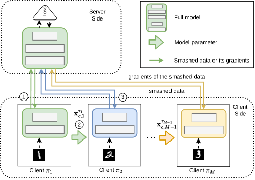
Figure 3: Overview of SSL in the peer-to-peer mode. The first three steps of the workflow: ① local updates with client $\pi_{1}$ (lines 8-15 of Alg. 3, lines 4-10 of Alg. 4); ② client-side model synchronization between clients $\pi_{1}$ and $\pi_{2}$, i.e., client $\pi_{1}$ sends the client-side local model parameters to client $\pi_{2}$; ③ local updates with client $\pi_{2}$.

In SL, the full model is split to be trained at the clients and server, where the portion at the client side is called the client-side model and the portion at the server is called the server-side model. In this section, we provide more operation details about SSL. All settings are the same as that in the main body except that varying number of local steps per client is adopted.

Operation details of SSL.

Figure 3 provides a overview of SSL. At the beginning of each training round, the indices $\pi_{1},\pi_{2},\ldots,\pi_{M}$ are sampled without replacement from $\{1,2,\ldots,M\}$ randomly as clients’ training order. The training process for any client $\tau_{m}$ can be divided into three parts.

Initialization. In each round, client $\tau_{m}$ and the server initialize their model parameters with the latest model parameters (line 3 of Alg. 4, line 6 of Alg. 3). Note that the server-side model is latest in practice, we specify here for clarity (to be consistent with the client side).

Local updates. The client and server perform multiple steps of local updates collaboratively (lines 4-10 of Alg. 4, lines 8-15 of Alg. 3). The local update process in SSL includes: (i) the client executes the forward pass with its local data samples. It sends the smashed data and labels to the server, where the smashed data is the activation of the cut layer (the last layer of the client-side model). (ii) After receiving the smashed data and labels, the server executes the forward pass on the server-side model with the smashed data as the input, computes the loss with the output of the server-side model and labels, executes the backward pass, sends the gradients of the smashed data to the client and updates its server-side model parameters. (iii) After receiving the gradients, the client continues to execute the backward pass and updates its client-side model parameters.

Client-side model synchronization. Client-side model parameters can be synchronized in two modes, the peer-to-peer mode and centralized mode (Gupta and Raskar, 2018). In the peer-to-peer mode, the updated client-side model parameters will be sent to the next client directly, as shown in Figure 3. In the centralized mode, the updated parameters will be sent to the next client with the server as a medium. We mark the differences of these two modes with pink and gray color box in Algs. 3, 4.

This process continues until all the clients finish their local updates. Details are given in Algorithms 3, 4. Additional notations required for operations of SSL are given in Table 5.

Table 5: Additional notations for Section D.

Symbol	Description
$\tau_{m},k$	number, index of local update steps (when training) with client $\pi_{m}$
${\mathbf{x}}_{m}^{(r,k)}$/${\mathbf{x}}_{c,m}^{(r,k)}$/${\mathbf{x}}_{s,m}^{(r,k)}$	full/client-side/server-side local model parameters (${\mathbf{x}}_{m}^{(r,k)}=[{\mathbf{x}}_{c,m}^{(r,k)};{\mathbf{x}}_{s,m}^{(r,k)}]$)    after $k$ local updates with client $\pi_{m}$ in the $r$-th round
${\bm{X}}_{m}^{(r,k)}$/${\bm{Y}}_{m}^{(r,k)}$/$\hat{\bm{Y}}_{m}^{(r,k)}$	features/labels/predictors    after $k$ local updates with client $\pi_{m}$ in the $r$-th round
${\mathbf{x}}^{r}$/${\mathbf{x}}_{c}^{r}$/${\mathbf{x}}_{s}^{r}$	full/client-side/server-side global model parameters in the $r$-th round
${\bm{A}}_{m}^{(r,k)}$	smashed data (activation of the cut layer)    after $k$ local updates with client $\pi_{m}$ in the $r$-th round
$\ell_{\pi_{m}}$	loss function with client $\pi_{m}$
$\nabla\ell_{\pi_{m}}({\mathbf{x}}_{s,m}^{(r,k)};{\bm{A}}_{m}^{(r,k)})$	gradients of the loss regarding ${\mathbf{x}}_{s,m}^{(r,k)}$ on input ${\bm{A}}_{m}^{(r,k)}$
$\nabla\ell_{\pi_{m}}({\bm{A}}_{m}^{(r,k)};{\mathbf{x}}_{s,m}^{(r,k)})$	gradients of the loss regarding ${\bm{A}}_{m}^{(r,k)}$ on parameters ${\mathbf{x}}_{s,m}^{(r,k)}$
$\nabla\ell_{\pi_{m}}({\mathbf{x}}_{c,m}^{(r,k)};{\bm{X}}_{m}^{(r,k)})$	gradients of the loss regarding ${\mathbf{x}}_{c,m}^{(r,k)}$ on input ${\bm{X}}_{m}^{(r,k)}$

Algorithm 3 SSL (Server-side operations) Peer-to-peer mode, Centralized mode

1:server-side global model parameters ${\mathbf{x}}_{s}^{r}={\mathbf{x}}_{s,M}^{(r-1,\tau_{M})}$.

2:procedure Main Server executes

3:     Initialize server-side global parameters ${\mathbf{x}}_{s}^{0}$

4:     for round $r=0,\ldots,R-1$ do

5:         Sample a permutation $\pi_{1},\pi_{2},\ldots,\pi_{M}$ of $\{1,2,\ldots,M\}$ as clients’ update order

6:         for $m=1,2,\ldots,M$ in sequence do

7:              Initialize server-side local parameters ${\mathbf{x}}_{s,m}^{(r,0)}\leftarrow\begin{cases}{\mathbf{x}}_{s}^{r},m=1\\ {\mathbf{x}}_{s,m-1}^{(r,\tau_{m-1})},m>1\end{cases}$

8:              Send ${\mathbf{x}}_{c,m-1}^{(r,\tau_{m-1})}$ to client $\tau_{m}$ (Centralized mode) $\triangleright$ Com.

9:              for local update step $k=0,\ldots,\tau_{m}-1$ do

10:                  Receive (${\bm{A}}_{m}^{(r,k)}$, ${\bm{Y}}_{m}^{(r,k)}$) from client $m$ $\triangleright$ Com.

11:                  Execute forward passes with smashed data ${\bm{A}}_{m}^{(r,k)}$

12:                  Calculate the loss with ($\hat{\bm{Y}}_{m}^{(r,k)}$, ${\bm{Y}}_{m}^{(r,k)}$)

13:                  Execute backward passes and compute $\nabla\ell_{\pi_{m}}({\mathbf{x}}_{s,m}^{(r,k)};{\bm{A}}_{m}^{(r,k)})$

14:                  Send $\nabla\ell_{\pi_{m}}({\bm{A}}_{m}^{(r,k)};{\mathbf{x}}_{s,m}^{(r,k)})$ to client $m$ $\triangleright$ Com.

15:                  Update server-side local parameters: ${\mathbf{x}}_{s,m}^{(r,k+1)}\leftarrow{\mathbf{x}}_{s,m}^{(r,k)}-\eta\nabla\ell_{\pi_{m}}({\mathbf{x}}_{s,m}^{(r,k)};{\bm{A}}_{m}^{(r,k)})$

16:              end for

17:              Receive ${\mathbf{x}}_{c,m}^{(r,\tau_{m})}$ from client $\tau_{m}$ (Centralized mode) $\triangleright$ Com.

18:         end for

19:     end for

20:end procedure

Algorithm 4 SSL (Client-side operations) Peer-to-peer mode, Centralized mode

1:client-side global model parameters ${\mathbf{x}}_{c}^{r}={\mathbf{x}}_{c,M}^{(r-1,\tau_{M})}$

2:procedure Client $\pi_{m}$ executes

3:     Request the lasted client-side parameters from the server, or the previous client $\triangleright$ Com.

4:     Initialize client-side local parameters ${\mathbf{x}}_{c,m}^{(r,0)}\leftarrow\begin{cases}{\mathbf{x}}_{c}^{r},m=1\\ {\mathbf{x}}_{c,m-1}^{(r,\tau_{m-1})},m>1\end{cases}$

5:     for local update step $k=0,\ldots,\tau_{m}-1$ do

6:         Execute forward passes with data features ${\bm{X}}_{m}^{(r,k)}$

7:         Send (${\bm{A}}_{m}^{(r,k)}$, ${\bm{Y}}_{m}^{(r,k)}$) to the server $\triangleright$ Com.

8:         Receive $\nabla\ell_{\pi_{m}}({\bm{A}}_{m}^{(r,k)};{\mathbf{x}}_{s,m}^{(r,k)})$ $\triangleright$ Com.

9:         Execute backward passes with $\nabla\ell_{\pi_{m}}({\bm{A}}_{m}^{(r,k)};{\mathbf{x}}_{s,m}^{(r,k)})$ and compute $\nabla\ell_{\pi_{m}}({\mathbf{x}}_{c,m}^{(r,k)};{\bm{X}}_{m}^{(r,k)})$

10:         Update client-side local parameters: ${\mathbf{x}}_{c,m}^{(r,k+1)}\leftarrow{\mathbf{x}}_{c,m}^{(r,k)}-\eta\nabla\ell_{\pi_{m}}({\mathbf{x}}_{c,m}^{(r,k)};{\bm{X}}_{m}^{(r,k)})$

11:     end for

12:     Send the updated client-side parameters ${\mathbf{x}}_{c,m}^{(r,\tau_{m})}$ to the server, or the next client $\triangleright$ Com.

13:end procedure

Appendix E Related work and limitations

Variants in SL.

SL is deemed as one promising paradigm for distributed learning at resource-constrained devices, given its computational efficiency on the client side. Most existing works focus on reducing the training delay arising from the relay-based training manner of vanilla SL in the multi-user scenario. SFLV1 (Thapa et al., 2020) is one popular model parallel algorithm that combines the strengths of FL and SL, where each client has one corresponding instance of server-side model in the main server to form a pair. Each pair constitutes a full model and conducts the local updates in parallel. After each training round, the fed server collects and averages the updated clien-side model parameters. The aggregated client-side model will be disseminated to all the clients before next round. The main server does the same operations to the instances of the server-side model (i.e., average the sever-side model parameters). SFLV2 (Thapa et al., 2020), SFLV3 (Gawali et al., 2020), SFLG (Gao et al., 2021) and FedSeq (Zaccone et al., 2022) are the variants of SFLV1.

Convergence analyses in SL.

The algorithm in Han et al. (2021) reduces the latency and downlink communication on SFLV1 by adding auxiliary networks at client-side for quick model updates. Their convergence analysis combines the theories of Belilovsky et al. (2020) and FedAvg. Wang et al. (2022b) proposed FedLite to reduce the uplink communication overhead by compressing activations with product quantization and provided the convergence analysis of FedLite. However, their convergence recovers that of Minibatch SGD when there is no quantization. SGD with biased gradients (Ajalloeian and Stich, 2020) is also related. However, it only converges to a neighborhood of the solution. As a result, the convergence of SSL on heterogeneous data is still lacking.

Limitations.

The limitations of our theory appearing in this paper are summarized: (i) As discussed in Section 4, the counterintuitive result that SSL outperforms FedAvg only hold in extremely heterogeneous settings (see Table 1), as FedAvg exhibits a better performance than existing theories suggest in moderately heterogeneous settings (Wang et al., 2022a). (ii) Some variants like SCAFFOLD (Karimireddy et al., 2020) show much better than FedAvg, which will be our future work. (iii) Other limitations will be same as the previous work in FL (Koloskova et al., 2020; Karimireddy et al., 2020) as standard assumptions are used for our theory.

Moreover, we discuss the limitations of SSL itself. One primary issue of SSL due to the sequential manner is the training time overhead (Thapa et al., 2020). Besides, SSL suffers from some privacy issues like label leakage (Li et al., 2021), which we believe is beyond the scope of this work.

Appendix F More experimental details

In this section, we provide more details about the experiments.

F.1 More simulations

Simulation validation on quadratic functions.

We adopt the one-dimensional quadratic functions as in Karimireddy et al. (2020) to validate the analysis above. To extend the simulated experiments in Section 4, 9 groups of experiments with the same global objective $F(x)=\frac{1}{2}x^{2}$ are considered. The detailed settings are in Table 6.

Notably, we use $\delta=\left\lVert\frac{1}{M}\sum_{m=1}^{M}x_{m}^{\ast}-x^{\ast}\right\rVert$ and $\zeta_{\ast}^{2}=\frac{1}{M}\sum_{m=1}^{M}\left\lVert\nabla F_{m}(x^{\ast})\right\rVert^{2}$ to measure heterogeneity, with a larger value meaning higher heterogeneity for both $\delta$ and $\zeta_{\ast}^{2}$, where $x_{m}^{\ast}$ is the local optimum of $F_{m}$ and $x^{\ast}$ is the global optimum.

Figure 4 plots the results of FedAvg and SSL with different values of $\delta$ and $\zeta_{\ast}$. The results validate that FedAvg performs much better than SSL (also better than Theorem 2 suggests) in moderately heterogeneous settings (see Groups 1-3, the first row in Figure 4) and worse than SSL in extremely heterogeneous settings (see Groups 4-9, the second and third rows in Figure 4).

Table 6: Settings of simulated experiments. Each group has two local objectives (i.e., $M=2$). We use $\delta=\left\lVert\frac{1}{M}\sum_{m=1}^{M}x_{m}^{\ast}-x^{\ast}\right\rVert$ and $\zeta_{\ast}^{2}=\frac{1}{M}\sum_{m=1}^{M}\left\lVert\nabla F_{m}(x^{\ast})\right\rVert^{2}$ to measure heterogeneity, with a larger value meaning higher heterogeneity for both $\delta$ and $\zeta_{\ast}^{2}$, where $x_{m}^{\ast}$ is the local optimum of $F_{m}$ and $x^{\ast}$ is the global optimum.

Settings	$F_{1}$	$F_{2}$	$\delta$	$\zeta_{\ast}$
Group 1	$F_{1}(x)=\frac{1}{2}x^{2}+x$	$F_{2}(x)=\frac{1}{2}x^{2}-x$	$0$	$1$
Group 2	$F_{1}(x)=\frac{1}{2}x^{2}+10x$	$F_{2}(x)=\frac{1}{2}x^{2}-10x$	$0$	$10$
Group 3	$F_{1}(x)=\frac{1}{2}x^{2}+100x$	$F_{2}(x)=\frac{1}{2}x^{2}-100x$	$0$	$100$
Group 4	$F_{1}(x)=\frac{2}{3}x^{2}+x$	$F_{2}(x)=\frac{1}{3}x^{2}-x$	$\frac{3}{8}$	$1$
Group 5	$F_{1}(x)=\frac{2}{3}x^{2}+10x$	$F_{2}(x)=\frac{1}{3}x^{2}-10x$	$\frac{3}{8}$	$10$
Group 6	$F_{1}(x)=\frac{2}{3}x^{2}+100x$	$F_{2}(x)=\frac{1}{3}x^{2}-100x$	$\frac{3}{8}$	$100$
Group 7	$F_{1}(x)=x^{2}+x$	$F_{2}(x)=-x$	$+\infty$	$1$
Group 8	$F_{1}(x)=x^{2}+10x$	$F_{2}(x)=-10x$	$+\infty$	$10$
Group 9	$F_{1}(x)=x^{2}+100x$	$F_{2}(x)=-100x$	$+\infty$	$100$

$\delta$=$0$

$\zeta_{\ast}=1$

$\zeta_{\ast}=10$

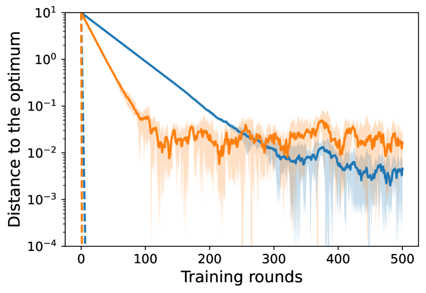
$\zeta_{\ast}=100$

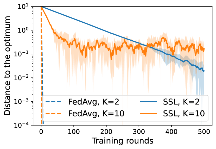
$\delta$=$\frac{3}{8}$

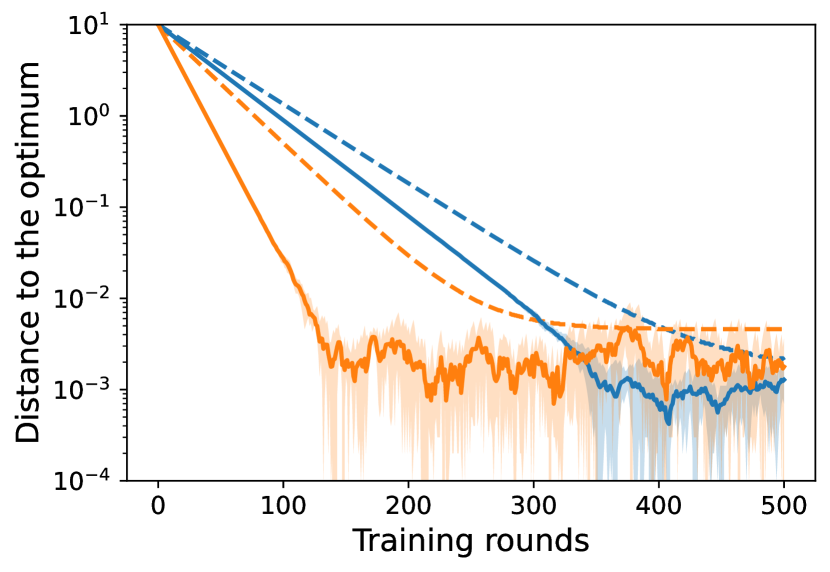
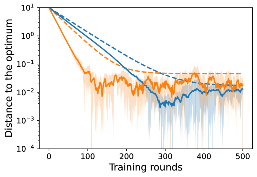
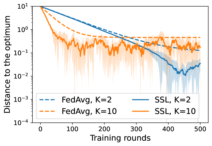
$\delta$=$\infty$

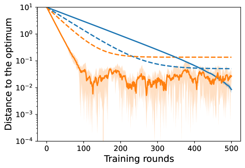
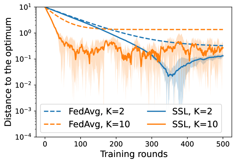
Figure 4: Simulations on quadratic functions. The first row shows the results of Groups 1-3 in Table 6. The second row shows the results of Groups 4-6. The third row shows the results of Groups 7-9. The best learning rates are chosen from [0.003, 0.006, 0.01, 0.03, 0.06, 0.1, 0.3, 0.6] with grid search. We run each experiments for 5 random seeds. Shaded areas show the min-max values.

F.2 Extended Dirichlet partition

Baseline.

The partition strategy based on the Dirichlet distribution has been widely used in the FL literature (Yurochkin et al., 2019; Hsu et al., 2019; Zhu et al., 2021; Wang et al., 2020; Jhunjhunwala et al., 2023). The initial implementation, to the best of our knowledge, comes from Yurochkin et al. (2019). They partition the dataset into $M$ clients. They simulate a heterogeneous partition by drawing ${\bm{p}}_{c}\sim\text{Dir}_{M}(\alpha)=\text{Dir}(\alpha{\bm{q}})$ and allocating a ${\bm{p}}_{c,m}$ proportion of the samples of class $k$ to client $m$. Here ${\bm{q}}$ is the prior distribution over $M$ clients, which is set as $\bm{1}\in\mathbb{R}^{M}$.

In the FL literature, there is another common partition strategy, where each client only owns samples from $C$ classes ($C\leq C_{\text{total}}$ and $C_{\text{total}}$ classes in total) (McMahan et al., 2017; Li et al., 2022). This partition strategy is pathological, which is used commonly in the personalized FL.

Extended Dirichlet strategy.

These two strategies prompt us to come up with a new two-level strategy, which combing the properties of both, to generate arbitrarily heterogeneous data.

The difference is to add a step of allocating classes to determine the number of classes per client (denoted by $C$) before allocating samples via Dirichlet distribution (with concentrate parameter $\alpha$). Thus, the extended strategy can be denoted by $\text{ExDir}(C,\alpha)$. Suppose that there are $M$ clients. The implementation is as follows:

• Allocating classes. Select $C$ classes for each client until each class is allocated to at least one client. Then we can obtain the prior distribution ${\bm{q}}_{c}\in\mathbb{R}^{M}$ over $M$ clients for any class $c$.

• Allocating samples. For any class $c$, we draw ${\bm{p}}_{c}\sim\text{Dir}(\alpha{\bm{q}}_{c})$ and then allocate a ${\bm{p}}_{c,m}$ proportion of the samples of class $c$ to client $m$. For example, ${\bm{q}}_{c}=[1,1,0,0,\ldots,]$ means that the samples of class $c$ are only allocated to the first 2 clients.

This strategy have two levels, the first level to allocate classes and the second level to allocate samples. Note that $C$ decides the prior distribution, yet it does not mean that every client must own samples from $C$ classes, which has shown in the following experiments. We note that Reddi et al. (2020) use a two-level partition strategy to partition the CIFAR-100 dataset. They draw a multinomial distribution from the Dirichlet prior at the root ($\text{Dir}(\alpha)$) and a multinomial distribution from the Dirichlet prior at each coarse label ($\text{Dir}(\beta)$).

We use the Extended Dirichlet strategy to partition samples from MNIST to 10 clients. The results are shown in Figure 5.

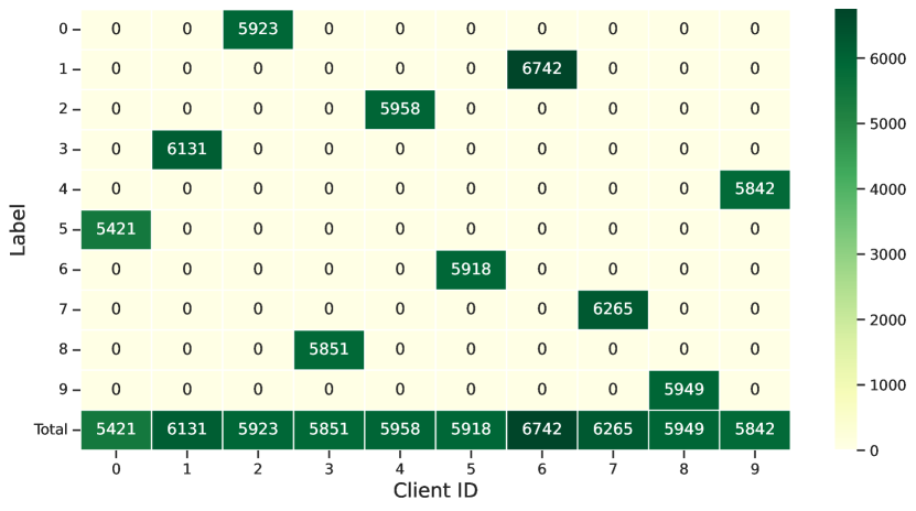
(a) 10 clients, $\text{ExDir}(1,100.0)$

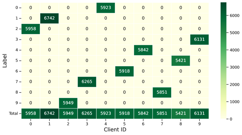
(b) 10 clients, $\text{ExDir}(1,10.0)$

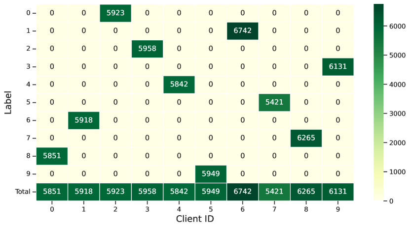
(c) 10 clients, $\text{ExDir}(1,1.0)$

(d) 10 clients, $\text{ExDir}(2,100.0)$

(e) 10 clients, $\text{ExDir}(2,10.0)$

(f) 10 clients, $\text{ExDir}(2,1.0)$

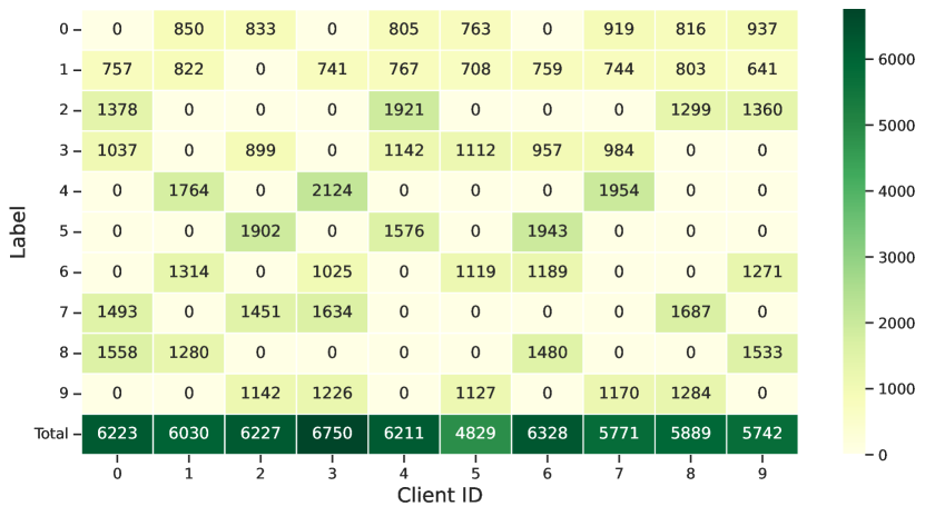
(g) 10 clients, $\text{ExDir}(5,100.0)$

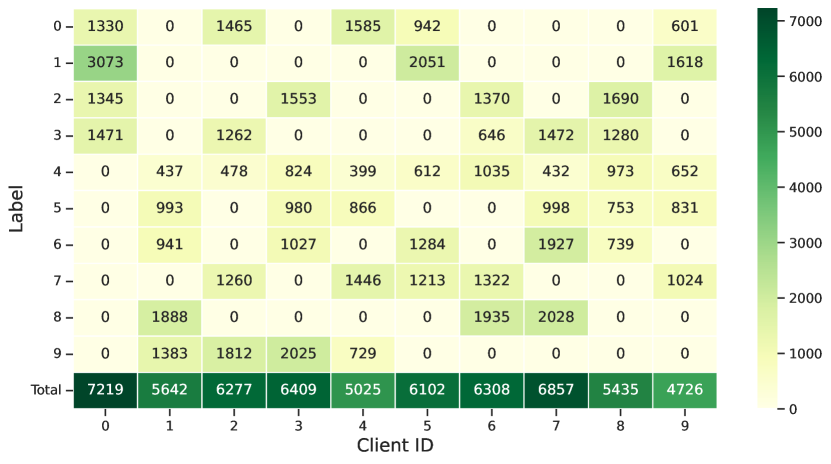
(h) 10 clients, $\text{ExDir}(5,10.0)$

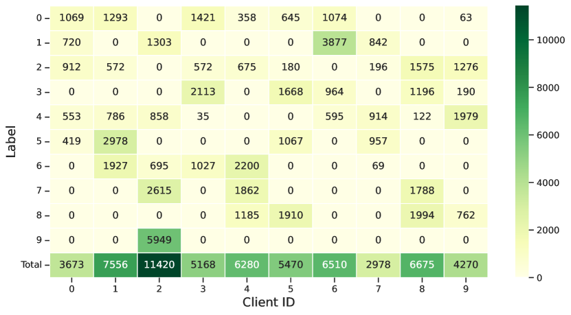
(i) 10 clients, $\text{ExDir}(5,1.0)$

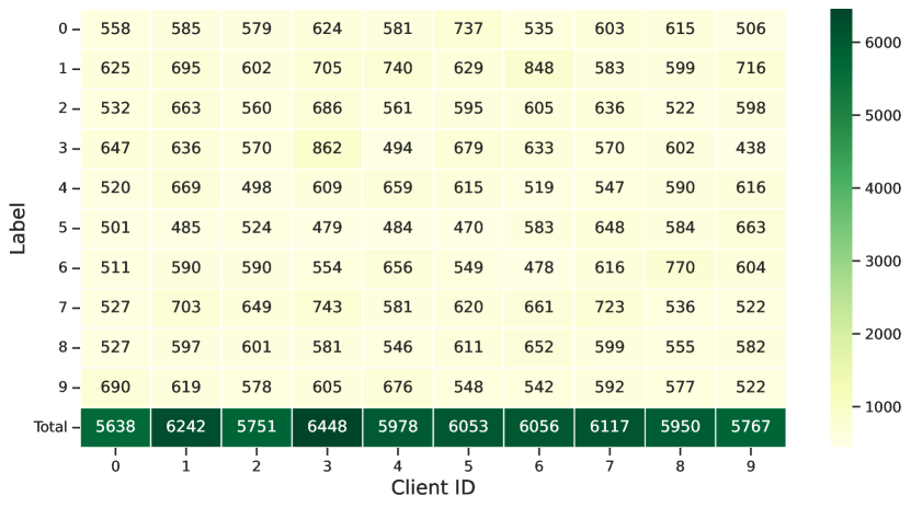
(j) 10 clients, $\text{ExDir}(10,100.0)$

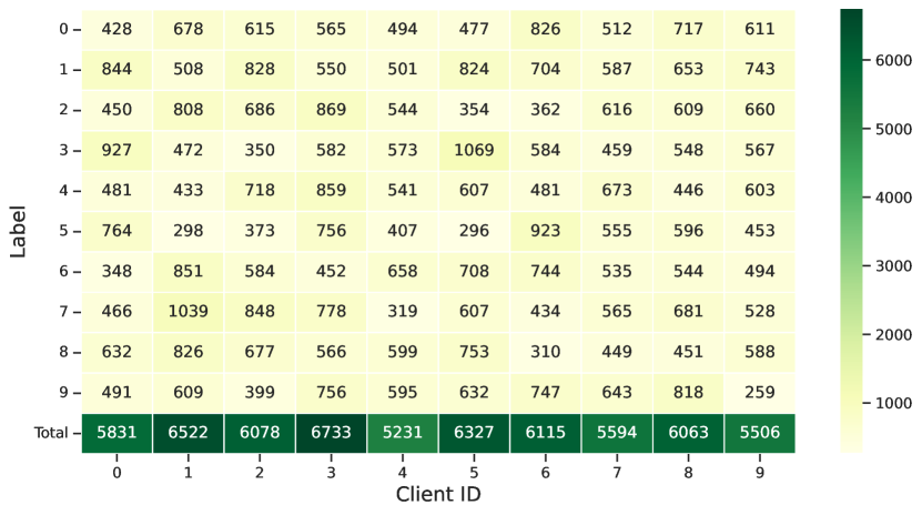
(k) 10 clients, $\text{ExDir}(10,10.0)$

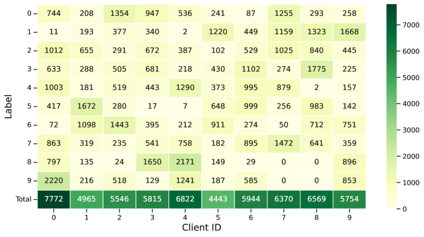
(l) 10 clients, $\text{ExDir}(10,1.0)$

Figure 5: Visualization of data heterogeneity. The x-axis indicates client IDs and the y-axis indicates labels. The value in each cell is the number of data samples of a label belonging to that client. For the first row, there are only one possible results in the case where each client owns one label with 10 clients and 10 labels in total, so these three partitions are the same. For the second, third and forth rows, data heterogeneity increases from left to right.

F.3 Hyperparameter details

Datasets and models.

We adopt the following models and datasets: (i) training LeNet-5 (LeCun et al., 1998) on the MNIST dataset (LeCun et al., 1998); (ii) training LeNet-5 on the FMNIST dataset (Xiao et al., 2017); (iii) training VGG-11 (Simonyan and Zisserman, 2014) on the CIFAR-10 dataset (Krizhevsky et al., 2009). For SL, the LeNet-5 is split after the second 2D MaxPool layer, with 6% of the entire model size retained in the client; the VGG-11 is split after the third 2D MaxPool layer, with 10% of the entire model size at the client. Ideally, the split layer position has no effect on the performance of SL (Wang et al., 2022b).

Platform.

We conducted all experiments with three different seeds 1234, 666, 22. The experiments of MNIST and FMNIST are conducted on Nvidia GeForce RTX 3090 with cuda 11.7, python 3.7, pytorch 1.13.1. The experiments of CIFAR-10 are conducted on NVIDIA GeForce RTX 4090 (seed 1234), Nvidia GeForce RTX 3090 (seeds 666, 22) with cuda 12.0, python 3.10, pytorch, pytorch 2.0.0+cu118.

Gradient clipping.

For $\text{ExDir}(2,10.0)$, we use the use gradient clipping with max norm = 10, to improve stability of the algorithms as done in previous work Acar et al. (2021); Jhunjhunwala et al. (2023) (the left plot in Figure 6). For $\text{ExDir}(1,10.0)$, we do not use gradient clipping as it hurts the convergence (the right plot in Figure 6).

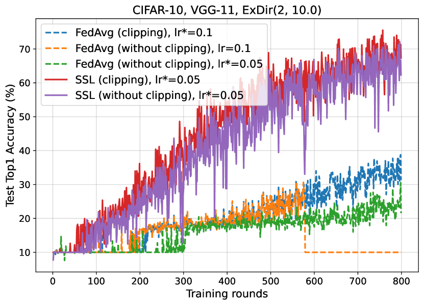
(a) $\text{Exdir}(2,10.0)$, $M=500$, $S=10$, $K=10$

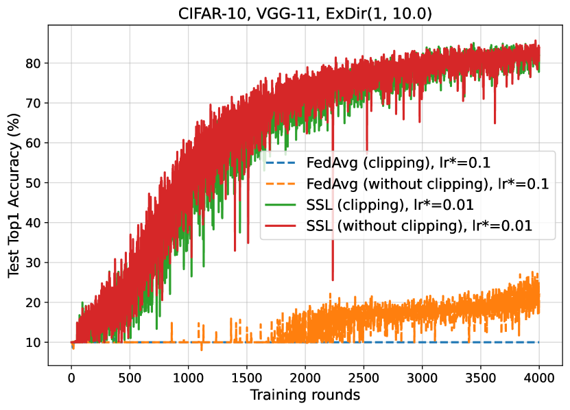
(b) $\text{Exdir}(1,10.0)$, $M=500$, $S=10$, $K=10$

Figure 6: Gradient clipping. “lr” in the legend represents the learning rate. “lr*” represents the best learning rate by the grid search. For the partitions $\text{ExDir}(2,10.0)$, we see gradient clipping improves the stability. It can mitigate the gradient explosion (the loss turns “Nan” in our experiments). Yet for the partition $\text{ExDir}(1,10.0)$, gradient clipping (max norm=10) hurts the convergence of both algorithms, especially FedAvg.

Other hyperparameters

The local optimizer is SGD with momentem = 0 and weight decay = 1e-4. No learning rate decay is used for all experiments. We fix the number of participating clients to be 10 and the mini-batch size to be 20 by default.

F.4 Grid search for learning rates

For all the algorithms, we use the grid search to find the best learning rate. Note that one random seed “1234” is used for all grid searches. We summarize the best learning rates of different setups in Table 7 and leave the details to the following subsubsections.

Table 7: Best learning rates for different setups.

Setup			$\text{ExDir}(1,10.0)$		$\text{ExDir}(2,10.0)$
			FedAvg	SSL	FedAvg	SSL
MNIST	$M=500$	$K=10$	0.001	0.01	0.05	0.05
		$K=20$	0.0005	0.01	0.05	0.05
FMNIST	$M=500$	$K=10$	0.001	0.01	0.1	0.1
		$K=20$	0.0005	0.01	0.1	0.05
CIFAR-10	$M=10$	$K=5$	0.5	0.01	0.1	0.05
		$K=10$	0.1	0.01	0.1	0.05
		$K=20$	0.1	0.01	0.1	0.01
		$K=30$	0.1	0.005	0.1	0.01
CIFAR-10	$M=500$	$K=5$	0.1	0.01	0.5	0.05
		$K=10$	0.1	0.01	0.1	0.05
		$K=20$	0.1	0.005	0.1	0.01
		$K=30$	-	-	0.1	0.01

F.5 More experimental results in cross-silo settings

Table 8: Test Accuracy results in cross-silo settings. We run 4000 rounds for both two partitions on CIFAR-10. Results are averaged across 3 random seeds and the last 20 rounds. The column 30% and 75% show the minimum number of rounds required to reach 30% and 75% accuracies.

Setup		$\text{ExDir}(1,10.0)$				$\text{ExDir}(2,10.0)$
		FedAvg		SSL		FedAvg		SSL
		ACC (%)	30%	ACC (%)	30%	ACC (%)	75%	ACC (%)	75%
CIFAR-10	$K=5$	$69.28\pm{\color[rgb]{.5,.5,.5}3.02}$	956	$84.79\pm{\color[rgb]{.5,.5,.5}0.45}$	495	$80.51\pm{\color[rgb]{.5,.5,.5}0.47}$	2413	$85.52\pm{\color[rgb]{.5,.5,.5}0.58}$	883
	$K=10$	$50.01\pm{\color[rgb]{.5,.5,.5}4.06}$	2254	$85.64\pm{\color[rgb]{.5,.5,.5}0.45}$	401	$80.91\pm{\color[rgb]{.5,.5,.5}0.58}$	1743	$84.33\pm{\color[rgb]{.5,.5,.5}0.66}$	897
	$K=20$	$25.30\pm{\color[rgb]{.5,.5,.5}2.72}$	3516	$84.75\pm{\color[rgb]{.5,.5,.5}0.51}$	712	$81.24\pm{\color[rgb]{.5,.5,.5}0.44}$	1236	$86.43\pm{\color[rgb]{.5,.5,.5}0.44}$	1096
	$K=30$	$32.07\pm{\color[rgb]{.5,.5,.5}5.95}$	3119	$83.19\pm{\color[rgb]{.5,.5,.5}0.79}$	920	$81.09\pm{\color[rgb]{.5,.5,.5}0.52}$	996	$85.48\pm{\color[rgb]{.5,.5,.5}0.61}$	1186

Figure 7: Test accuracy results with varying number of local steps on CIFAR-10 in cross-silo settings. We report the test accuracy results every 5 training rounds for clarity. The shaded areas show the standard deviation.

F.6 More experimental results in cross-device settings

Table 9: Test Accuracy results in cross-device settings. 1000 rounds are run for $\text{ExDir}(1,10.0)$ and 400 rounds for $\text{ExDir}(2,10.0)$ on MNIST, FMNIST. 4000 rounds are for both two partitions on CIFAR-10. Results are averaged across 3 random seeds and the last 20 rounds. The column 30% and 75% show the minimum number of rounds required to reach 30% and 75% accuracies.

Setup		$\text{ExDir}(1,10.0)$				$\text{ExDir}(2,10.0)$
		FedAvg		SSL		FedAvg		SSL
		ACC (%)	30%	ACC (%)	30%	ACC (%)	75%	ACC (%)	75%
CIFAR-10	$K=5$	$29.06\pm{\color[rgb]{.5,.5,.5}6.46}$	3666	$\textbf{81.34}\pm{\color[rgb]{.5,.5,.5}1.35}$	604	$75.92\pm{\color[rgb]{.5,.5,.5}1.17}$	3210	$\textbf{84.57}\pm{\color[rgb]{.5,.5,.5}0.90}$	1004
	$K=10$	$14.00\pm{\color[rgb]{.5,.5,.5}5.66}$	-	$\textbf{82.20}\pm{\color[rgb]{.5,.5,.5}1.33}$	483	$81.17\pm{\color[rgb]{.5,.5,.5}0.55}$	2153	$\textbf{82.95}\pm{\color[rgb]{.5,.5,.5}1.70}$	966
	$K=20$	$10.00\pm{\color[rgb]{.5,.5,.5}0.00}$	-	$\textbf{80.60}\pm{\color[rgb]{.5,.5,.5}1.62}$	673	$81.26\pm{\color[rgb]{.5,.5,.5}0.60}$	1614	$\textbf{85.24}\pm{\color[rgb]{.5,.5,.5}0.79}$	998
	$K=30$	-	-	-	-	$80.47\pm{\color[rgb]{.5,.5,.5}0.69}$	1618	$\textbf{84.52}\pm{\color[rgb]{.5,.5,.5}0.86}$	966
FMNIST	$K=10$	$39.90\pm{\color[rgb]{.5,.5,.5}6.08}$	492	$\textbf{80.38}\pm{\color[rgb]{.5,.5,.5}2.80}$	19	$\textbf{81.77}\pm{\color[rgb]{.5,.5,.5}1.15}$	127	$78.25\pm{\color[rgb]{.5,.5,.5}2.28}$	162
	$K=20$	$38.78\pm{\color[rgb]{.5,.5,.5}6.51}$	490	$\textbf{76.39}\pm{\color[rgb]{.5,.5,.5}3.15}$	25	$\textbf{83.55}\pm{\color[rgb]{.5,.5,.5}1.13}$	87	$76.58\pm{\color[rgb]{.5,.5,.5}3.18}$	103
MNIST	$K=10$	$56.43\pm{\color[rgb]{.5,.5,.5}11.54}$	274	$\textbf{98.84}\pm{\color[rgb]{.5,.5,.5}0.19}$	16	$98.15\pm{\color[rgb]{.5,.5,.5}0.13}$	25	$98.57\pm{\color[rgb]{.5,.5,.5}0.36}$	10
	$K=20$	$51.86\pm{\color[rgb]{.5,.5,.5}10.66}$	274	$\textbf{98.85}\pm{\color[rgb]{.5,.5,.5}0.12}$	14	$98.35\pm{\color[rgb]{.5,.5,.5}0.14}$	18	$98.56\pm{\color[rgb]{.5,.5,.5}0.33}$	8

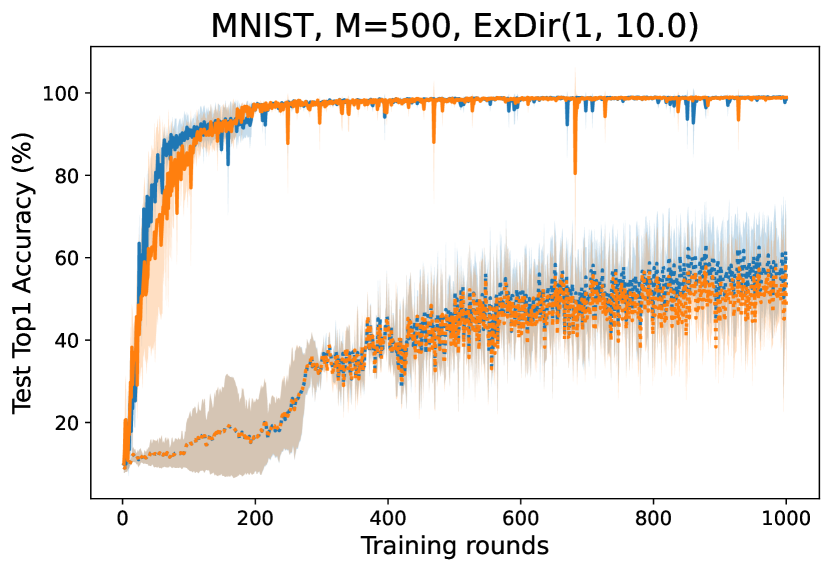
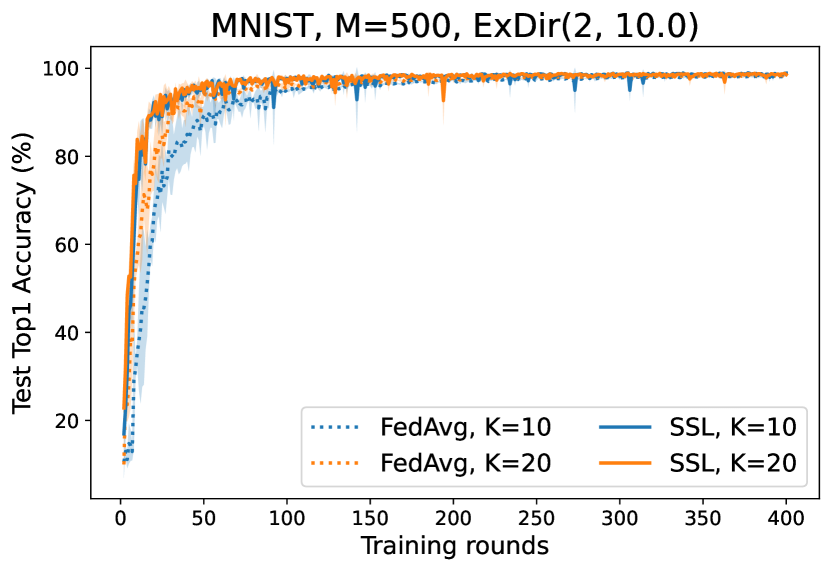
Figure 8: Test accuracy results with varying number of local steps on MNIST in cross-device settings. The shaded areas show the standard deviation.

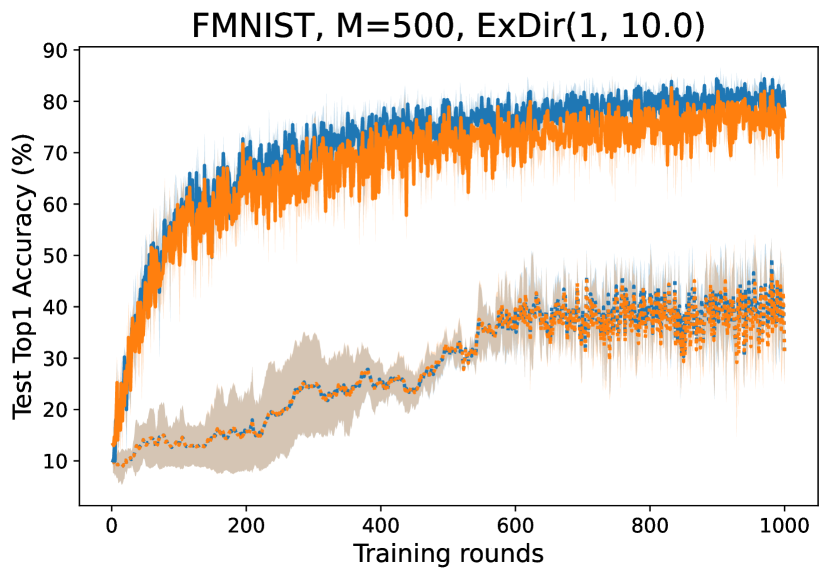
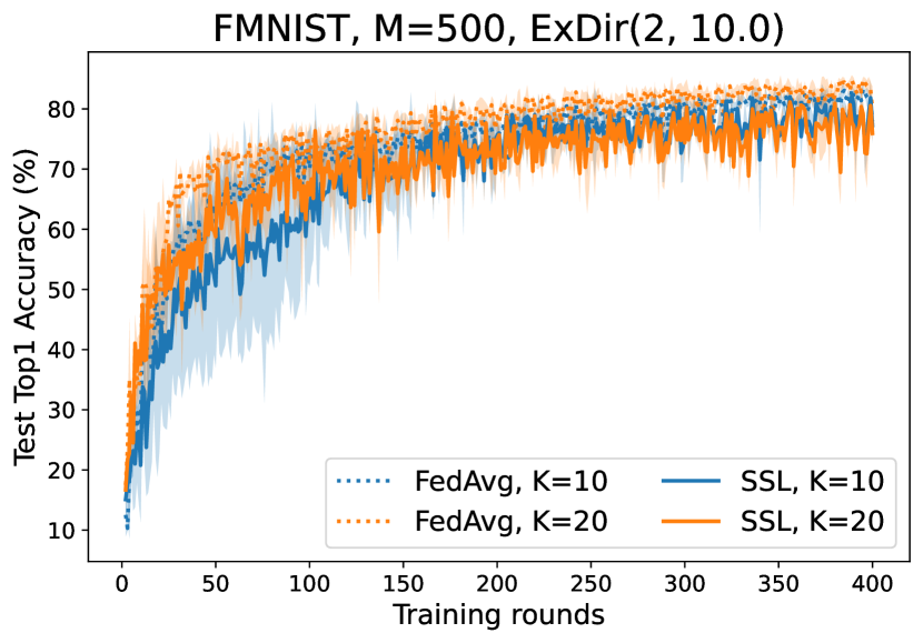
Figure 9: Test accuracy results with varying number of local steps on FMNIST in cross-device settings. The shaded areas show the standard deviation.

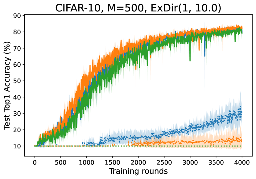
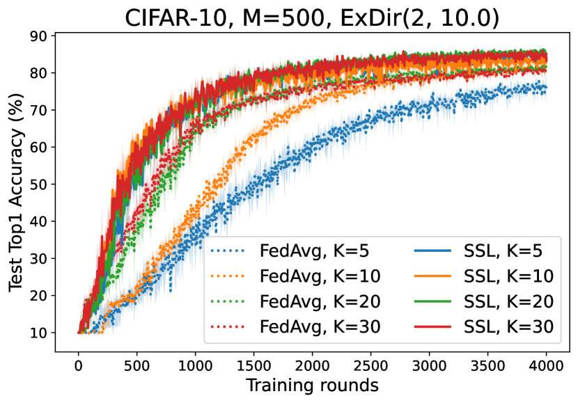
Figure 10: Test accuracy results with varying number of local steps on CIFAR-10 in cross-device settings. We report the test accuracy results every 5 training rounds for clarity. The shaded areas show the standard deviation.

References

- Acar et al. (2021) Durmus Alp Emre Acar, Yue Zhao, Ramon Matas Navarro, Matthew Mattina, Paul N Whatmough, and Venkatesh Saligrama. Federated learning based on dynamic regularization. arXiv preprint arXiv:2111.04263, 2021.
- Ajalloeian and Stich (2020) Ahmad Ajalloeian and Sebastian U Stich. On the convergence of sgd with biased gradients. arXiv preprint arXiv:2008.00051, 2020.
- Belilovsky et al. (2020) Eugene Belilovsky, Michael Eickenberg, and Edouard Oyallon. Decoupled greedy learning of CNNs. In International Conference on Machine Learning, pages 736–745. PMLR, 2020.
- Bottou et al. (2018) Léon Bottou, Frank E Curtis, and Jorge Nocedal. Optimization methods for large-scale machine learning. Siam Review, 60(2):223–311, 2018.
- Boyd et al. (2004) Stephen Boyd, Stephen P Boyd, and Lieven Vandenberghe. Convex optimization. Cambridge university press, 2004. URL https://web.stanford.edu/~boyd/cvxbook/bv_cvxbook.pdf.
- Caldas et al. (2018) Sebastian Caldas, Sai Meher Karthik Duddu, Peter Wu, Tian Li, Jakub Konečnỳ, H Brendan McMahan, Virginia Smith, and Ameet Talwalkar. Leaf: A benchmark for federated settings. arXiv preprint arXiv:1812.01097, 2018.
- Fraboni et al. (2021) Yann Fraboni, Richard Vidal, Laetitia Kameni, and Marco Lorenzi. Clustered sampling: Low-variance and improved representativity for clients selection in federated learning. In International Conference on Machine Learning, pages 3407–3416. PMLR, 2021.
- Gao et al. (2020) Yansong Gao, Minki Kim, Sharif Abuadbba, Yeonjae Kim, Chandra Thapa, Kyuyeon Kim, Seyit A Camtepe, Hyoungshick Kim, and Surya Nepal. End-to-end evaluation of federated learning and split learning for internet of things. arXiv preprint arXiv:2003.13376, 2020.
- Gao et al. (2021) Yansong Gao, Minki Kim, Chandra Thapa, Sharif Abuadbba, Zhi Zhang, Seyit Camtepe, Hyoungshick Kim, and Surya Nepal. Evaluation and optimization of distributed machine learning techniques for internet of things. IEEE Transactions on Computers, 2021.
- Garrigos and Gower (2023) Guillaume Garrigos and Robert M Gower. Handbook of convergence theorems for (stochastic) gradient methods. arXiv preprint arXiv:2301.11235, 2023.
- Gawali et al. (2020) Manish Gawali, Shriya Suryavanshi, Harshit Madaan, Ashrika Gaikwad, Bhanu Prakash KN, Viraj Kulkarni, Aniruddha Pant, et al. Comparison of privacy-preserving distributed deep learning methods in healthcare. arXiv preprint arXiv:2012.12591, 2020.
- Gupta and Raskar (2018) Otkrist Gupta and Ramesh Raskar. Distributed learning of deep neural network over multiple agents. Journal of Network and Computer Applications, 116:1–8, 2018.
- Han et al. (2021) Dong-Jun Han, Jaekyun Moon, Hasnain Irshad Bhatti, and Jungmoon Lee. Accelerating federated learning with split learning on locally generated losses. In ICML 2021 Workshop on Federated Learning for User Privacy and Data Confidentiality. ICML Board, 2021.
- Hsu et al. (2019) Tzu-Ming Harry Hsu, Hang Qi, and Matthew Brown. Measuring the effects of non-identical data distribution for federated visual classification. arXiv preprint arXiv:1909.06335, 2019.
- Jhunjhunwala et al. (2023) Divyansh Jhunjhunwala, Shiqiang Wang, and Gauri Joshi. Fedexp: Speeding up federated averaging via extrapolation. arXiv preprint arXiv:2301.09604, 2023.
- Kairouz et al. (2021) Peter Kairouz, H Brendan McMahan, Brendan Avent, Aurélien Bellet, Mehdi Bennis, Arjun Nitin Bhagoji, Kallista Bonawitz, Zachary Charles, Graham Cormode, Rachel Cummings, et al. Advances and open problems in federated learning. Foundations and Trends® in Machine Learning, 14(1–2):1–210, 2021.
- Karimireddy et al. (2020) Sai Praneeth Karimireddy, Satyen Kale, Mehryar Mohri, Sashank Reddi, Sebastian Stich, and Ananda Theertha Suresh. Scaffold: Stochastic controlled averaging for federated learning. In International Conference on Machine Learning, pages 5132–5143. PMLR, 2020.
- Khaled et al. (2020) Ahmed Khaled, Konstantin Mishchenko, and Peter Richtárik. Tighter theory for local sgd on identical and heterogeneous data. In International Conference on Artificial Intelligence and Statistics, pages 4519–4529. PMLR, 2020.
- Koloskova et al. (2020) Anastasia Koloskova, Nicolas Loizou, Sadra Boreiri, Martin Jaggi, and Sebastian Stich. A unified theory of decentralized sgd with changing topology and local updates. In International Conference on Machine Learning, pages 5381–5393. PMLR, 2020.
- Krizhevsky et al. (2009) Alex Krizhevsky et al. Learning multiple layers of features from tiny images. Technical report, 2009.
- LeCun et al. (1998) Yann LeCun, Léon Bottou, Yoshua Bengio, and Patrick Haffner. Gradient-based learning applied to document recognition. Proceedings of the IEEE, 86(11):2278–2324, 1998.
- Li et al. (2021) Oscar Li, Jiankai Sun, Xin Yang, Weihao Gao, Hongyi Zhang, Junyuan Xie, Virginia Smith, and Chong Wang. Label leakage and protection in two-party split learning. arXiv preprint arXiv:2102.08504, 2021.
- Li et al. (2022) Qinbin Li, Yiqun Diao, Quan Chen, and Bingsheng He. Federated learning on non-iid data silos: An experimental study. In 2022 IEEE 38th International Conference on Data Engineering (ICDE), pages 965–978. IEEE, 2022.
- Li et al. (2019) Xiang Li, Kaixuan Huang, Wenhao Yang, Shusen Wang, and Zhihua Zhang. On the convergence of fedavg on non-iid data. arXiv preprint arXiv:1907.02189, 2019.
- McMahan et al. (2017) Brendan McMahan, Eider Moore, Daniel Ramage, Seth Hampson, and Blaise Aguera y Arcas. Communication-efficient learning of deep networks from decentralized data. In Artificial intelligence and statistics, pages 1273–1282. PMLR, 2017.
- Mishchenko et al. (2020) Konstantin Mishchenko, Ahmed Khaled, and Peter Richtárik. Random reshuffling: Simple analysis with vast improvements. Advances in Neural Information Processing Systems, 33:17309–17320, 2020.
- Orabona (2019) Francesco Orabona. A modern introduction to online learning. arXiv preprint arXiv:1912.13213, 2019.
- Reddi et al. (2020) Sashank Reddi, Zachary Charles, Manzil Zaheer, Zachary Garrett, Keith Rush, Jakub Konečnỳ, Sanjiv Kumar, and H Brendan McMahan. Adaptive federated optimization. arXiv preprint arXiv:2003.00295, 2020.
- Safran and Shamir (2020) Itay Safran and Ohad Shamir. How good is sgd with random shuffling? In Conference on Learning Theory, pages 3250–3284. PMLR, 2020.
- Safran and Shamir (2021) Itay Safran and Ohad Shamir. Random shuffling beats sgd only after many epochs on ill-conditioned problems. Advances in Neural Information Processing Systems, 34:15151–15161, 2021.
- Simonyan and Zisserman (2014) Karen Simonyan and Andrew Zisserman. Very deep convolutional networks for large-scale image recognition. arXiv preprint arXiv:1409.1556, 2014.
- Singh et al. (2019) Abhishek Singh, Praneeth Vepakomma, Otkrist Gupta, and Ramesh Raskar. Detailed comparison of communication efficiency of split learning and federated learning. arXiv preprint arXiv:1909.09145, 2019.
- Stich (2019a) Sebastian U Stich. Unified optimal analysis of the (stochastic) gradient method. arXiv preprint arXiv:1907.04232, 2019a.
- Stich and Karimireddy (2019) Sebastian U. Stich and Sai Praneeth Karimireddy. The Error-Feedback Framework: Better Rates for SGD with Delayed Gradients and Compressed Communication. arXiv preprint arXiv:1909.05350, 2019.
- Stich (2019b) Sebastian Urban Stich. Local SGD converges fast and communicates little. International Conference on Learning Representations (ICLR), page arXiv:1805.09767, 2019b. URL https://arxiv.org/abs/1805.09767.
- Thapa et al. (2020) Chandra Thapa, Mahawaga Arachchige Pathum Chamikara, Seyit Camtepe, and Lichao Sun. Splitfed: When federated learning meets split learning. arXiv preprint arXiv:2004.12088, 2020.
- Vepakomma et al. (2018) Praneeth Vepakomma, Otkrist Gupta, Tristan Swedish, and Ramesh Raskar. Split learning for health: Distributed deep learning without sharing raw patient data. arXiv preprint arXiv:1812.00564, 2018.
- Wang et al. (2020) Jianyu Wang, Qinghua Liu, Hao Liang, Gauri Joshi, and H Vincent Poor. Tackling the objective inconsistency problem in heterogeneous federated optimization. Advances in neural information processing systems, 33:7611–7623, 2020.
- Wang et al. (2022a) Jianyu Wang, Rudrajit Das, Gauri Joshi, Satyen Kale, Zheng Xu, and Tong Zhang. On the unreasonable effectiveness of federated averaging with heterogeneous data. arXiv preprint arXiv:2206.04723, 2022a.
- Wang et al. (2022b) Jianyu Wang, Hang Qi, Ankit Singh Rawat, Sashank Reddi, Sagar Waghmare, Felix X Yu, and Gauri Joshi. Fedlite: A scalable approach for federated learning on resource-constrained clients. arXiv preprint arXiv:2201.11865, 2022b.
- Woodworth et al. (2020) Blake E Woodworth, Kumar Kshitij Patel, and Nati Srebro. Minibatch vs local sgd for heterogeneous distributed learning. Advances in Neural Information Processing Systems, 33:6281–6292, 2020.
- Xiao et al. (2017) Han Xiao, Kashif Rasul, and Roland Vollgraf. Fashion-mnist: a novel image dataset for benchmarking machine learning algorithms. arXiv preprint arXiv:1708.07747, 2017.
- Yang et al. (2021) Haibo Yang, Minghong Fang, and Jia Liu. Achieving linear speedup with partial worker participation in non-iid federated learning. arXiv preprint arXiv:2101.11203, 2021.
- Yu et al. (2020) Felix Yu, Ankit Singh Rawat, Aditya Menon, and Sanjiv Kumar. Federated learning with only positive labels. In International Conference on Machine Learning, pages 10946–10956. PMLR, 2020.
- Yurochkin et al. (2019) Mikhail Yurochkin, Mayank Agarwal, Soumya Ghosh, Kristjan Greenewald, Nghia Hoang, and Yasaman Khazaeni. Bayesian nonparametric federated learning of neural networks. In International conference on machine learning, pages 7252–7261. PMLR, 2019.
- Zaccone et al. (2022) Riccardo Zaccone, Andrea Rizzardi, Debora Caldarola, Marco Ciccone, and Barbara Caputo. Speeding up heterogeneous federated learning with sequentially trained superclients. arXiv preprint arXiv:2201.10899, 2022.
- Zhou and Cong (2017) Fan Zhou and Guojing Cong. On the convergence properties of a -step averaging stochastic gradient descent algorithm for nonconvex optimization. arXiv preprint arXiv:1708.01012, 2017.
- Zhou (2018) Xingyu Zhou. On the fenchel duality between strong convexity and lipschitz continuous gradient. arXiv preprint arXiv:1803.06573, 2018.
- Zhu et al. (2021) Zhuangdi Zhu, Junyuan Hong, and Jiayu Zhou. Data-free knowledge distillation for heterogeneous federated learning. In International Conference on Machine Learning, pages 12878–12889. PMLR, 2021.