Stability of local tip pool sizes

Abstract.

In distributed ledger technologies (DLTs) with a directed acyclic graph (DAG) data structure, a block-issuing node can decide where to append new blocks and, consequently, how the DAG grows. This DAG data structure is typically decomposed into two pools of blocks, dependent on whether another block already references them. The unreferenced blocks are called the tips. Due to network delay, nodes can perceive the set of tips differently, giving rise to local tip pools.

We present a new mathematical model to analyse the stability of the different local perceptions of the tip pools and allow heterogeneous and random network delay in the underlying peer-to-peer communication layer. Under natural assumptions, we prove that the number of tips is ergodic, converges to a stationary distribution, and provide quantitative bounds on the tip pool sizes. We conclude our study with agent-based simulations to illustrate the convergence of the tip pool sizes and the pool sizes’ dependence on the communication delay and degree of centralization.

1. Introduction

A major challenge in distributed systems is the relativity of simultaneity and the fact that whether two spatially separated events occur simultaneously or in a particular order is not absolute but depends on the local perceptions of the participants. To fight this phenomenon, classical approaches in distributed ledger technologies (DLTs) such as Bitcoin [27] typically use a totally ordered data structure, a blockchain, to find consensus on the order of the events. However, this design creates a bottleneck, e.g. a miner or validator, through which each transaction must pass. And even in this solution, due to network delay, block creation can happen concurrently at different parts of the network, leading to bifurcations of the chain that must be resolved. This resolution is typically made by the longest–chain rule [27], or some variant of the heaviest sub-tree [39].

In blockchain-like DLTs, the system’s throughput is artificially limited to guarantee the system’s security so that each block propagates to all the participants before the next block is created. The blocks are created by miners or validators, and the blockchain can be seen as a three-step process. In the first step, a client sends a transaction to the block producers, then a particular block producer, also called the “leader”, proposes a block containing a batch of transactions, and in the last step, validators validate the block.

A more novel approach that addresses the limited throughput problem and the bifurcation of the chain problem of distributed ledgers uses a directed acyclic graph (DAG) instead of a chain to encode the dependencies of the blocks. For instance, protocols like SPECTRE [37], Byteball [5], Algorand [13], PHANTOM [38], Prism [3], Aleph [14], Narwhal [8], and IOTA [34]) were proposed to improve the performance of distributed ledgers. The consensus mechanism and the writing access in a DAG-based system can be conceptually different from the one in a linear blockchain system, and the transaction throughput is potentially no longer limited. For instance, in DAG-based protocols like Aleph [14] and Narwhal [8], only a predefined set of nodes can add new blocks to the ledger, while in IOTA [26], every participant has writing access.

We consider the more general model where every participant can add blocks to the data structure, referring to at least two previous blocks. This property reduces the update of the ledger to two steps: one node proposes a block to the ledger and waits for the other nodes to validate it, i.e., by adding a new block referencing them. This collaborative design in which all participants play the same role promises to mitigate (or even solve) several problems of the blockchain design, e.g., mining races [9], centralisation [25], miner extractable value [7], and negative externalities [36]. However, the parallelism in adding new blocks to the ledger implies that local perceptions of the nodes may differ much more than in the traditional blockchain design.

In this paper, we give a mathematical model describing the evolution of the local number of unreferenced blocks, or tips, in a distributed ledger and prove their stability. More precisely, we prove the stationarity and ergodicity of the number of tips. Except for [20], this model is new, as previous research neglected the difference between local perceptions due to heterogeneous network delays. In [20], a similar, but much more restrictive, model has been considered with deterministic delay, deterministic arrival of blocks and discrete time. This paper considers a continuous time model with random block creation and random delays. In the next section, we give an informal description of the model.

1.1. Informal description

We consider a network of nodes that manage a distributed database. In cryptocurrency applications, this database is called a ledger, but the model could potentially be applied to other use cases of collaborative databases. The data consists of blocks that contain atomic data in the sense that either the entire block is added to the database or all the information in the block is discarded. The distributed ledger is assumed to be built using two fundamental mechanisms:

Sharing mechanism: Each node aims to create new blocks and inform the other nodes about these blocks. The information about the blocks is passed via a gossip protocol on an underlying communication layer. Specifically, each node is only directly connected to a subset of the other nodes. Once a node has created a block and added it to its local database, it broadcasts it to a random subset of its neighbours. As soon as a node receives a block that it has not yet received, it adds this block to its database and forwards it to a random subset of its neighbours.

Reference mechanism: The blocks in the database (which we referred to also as vertices) are connected to each other by references. The rule is that each newly created block must refer to up to $k\geq 2$ already existing blocks. The meaning of these references can depend on the specific use case of the protocol. For example, in cryptocurrency applications, a reference of a block means that the node issuing the referencing transaction verifies the previous blocks. Verification includes semantic and syntactical checks of the block content. In addition, referencing a block can be used for validation and consensus building; see IOTA, [33], and IOTA 2.0, [26]. In distributed-queuing theory, blocks can correspond to different jobs. Referencing can then imply that the issuing node handles or will handle the jobs in the referenced blocks. The way nodes choose previously referenced blocks has an impact on the performance of the system. In particular, previously referenced blocks should no longer be referenced. Instead, the focus should be on referencing non-referenced blocks, which we call tips.

Regarding the reference mechanism, we can note that the delay between nodes has a huge impact on the performance of the reference mechanism. Indeed, it is instructive to consider the extreme case where all nodes have the same perception of the database. This can be the case when the creation of a block is instantaneous, i.e., there is no delay between selecting the references of the block and sending it to the neighbours, and all neighbours receive the new blocks without delay. Suppose we start the database with one block (the genesis) and assume that no blocks can be created simultaneously. In that case, there will always be only one tip (non-referenced block), as each block is referenced by precisely one other block. However, this situation changes drastically if there is a delay between the selection of references and the time when all nodes have received the new block. In this case, the blocks are created concurrently, and the blocks can be referenced by more than one other block. Thus, a prior, it is no longer clear whether the system is in a stationary regime or the number of tips explodes. In this paper, we propose a mathematical procedure to model the different local tip tools and prove the stability of their sizes under standard synchrony assumptions.

1.2. Contributions

This paper has three major contributions:

1. We formalize the above description of the (distributed) protocol using an appropriate stochastic process. This is the first continuous-time model for local perceptions of a DAG-based distributed ledger together with the communication on the underlying peer-to-peer network.

2. Our main result, Theorem 3.10, is a formal proof of the stability of the local tip pool sizes. The proof relies on an asymptotic drift analysis, Theorem 3.1, that allows, together with a regeneration structure, to obtain qualitative results on the stationarity and ergodicity of the local tip pools.

3. Finally, through Monte-Carlo simulations, we provide more quantitative results highlighting the influence of the protocols environment on the differences in the local perceptions.

1.3. Related work

To the best of our knowledge, S. Popov introduced the first mathematical model on DAG-based ledgers [33]. Popov’s analysis is based on a global and perfect observation of the existing blocks. The communication delay is assumed to be homogeneous, and newly created blocks can be referenced only after a given constant network delay. The author heuristically obtains a formula for the expected number of tips assuming that the tip pool size is stationary.

Under the above assumptions of the existence of a central node, a lot of works have extended the work of Popov, studying non-Poisson arrival rate [23], fluid limit approximations of the evolution of the number of tips [11, 12], discrete-time model [4], and simulation-based works [21, 28]. One of the main drawbacks of all these works is that they do not consider heterogeneous delays between nodes.

Three recent works have introduced different types of heterogeneous delays and studied the evolution of the number of tips under such conditions. First, a simulator of DAG-based distributed ledgers with delays in the transmission of information between nodes has been proposed in [41]. From a more theoretical perspective, the authors in [31] have studied the impact of heterogeneous delays coming from different processing times of the blocks and not due to propagation of information delay. They also assume the existence of a central node which maintains a stable version of the ledger and have not considered the different views of each node in the network. Our work is building on the model proposed in [20]. In that paper, the authors model the evolution of the number of tips using coupled stochastic processes in discrete time. However, [20] makes strong assumptions; the delay between two nodes is deterministic and constant over time and the number of issued blocks by each node at each discrete time-step is constant. Under these conditions, they prove the stability of the stochastic process using super martingale arguments and drift analysis.

2. Notations and setting

Variable	Description
${\mathcal{N}}:=\{1,\ldots,N\}$	set of nodes
$\lambda_{i}\in\mathbb{R}_{+}$	block issuance rate of node $i$
$\lambda:=\sum_{i=1}^{N}\lambda_{i}$	total block issuance rate
${\delta}_{j}^{({b})}(i)$	random variable describing
	latency from node $j$ to node $i$ for block ${b}$
$\Delta_{j}(i)$	latency distribution from node $j$ to node $i$
$\Delta\in\mathbb{R}_{+}$	maximal latency between two nodes
$k$	number of blocks to be referenced by a new block
$\mathrm{pool}_{n}^{(i)}$	tip pool of node $i$ at time $t_{n}$
$\mathrm{pool}_{n}^{(c)}$	common tip pool at time $t_{n}$
$\mathrm{pool}_{n}^{(o)}$	tips of the perfect observer at time $t_{n}$
$X_{n}^{(i)}:=\lvert\mathrm{pool}_{n}^{(i)}\rvert$	size of the tip pool of node $i$
$X_{n}^{(c)}:=\lvert\mathrm{pool}_{n}^{(c)}\lvert$	size of the common tip pool
$X_{n}^{(o)}:=\lvert\mathrm{pool}_{n}^{(o)}\rvert$	size of the tip pool of the perfect observer

Table 1. Table of notations

2.1. Peer-to-peer network

There are several factors that should be considered when modelling a peer-to-peer (P2P) network, including the number and distribution of participants, the speed and capacity of the network connections, and the rules governing the creation and exchange of data.

We consider a peer-to-peer network with $N$ nodes and denote the set of nodes by ${\mathcal{N}}:=\{1,\ldots,N\}$. These nodes can create (or issue) and exchange blocks of data without the need of a central authority.

Nodes communicate their blocks on the P2P network, leading to communication delays and, thus, different local perceptions of the system’s state. The network latency is the time it takes for a block to travel from the source node to the destination node and can be affected by a number of factors, including the distance between the two nodes, the speed of the network connection, and the amount of traffic on the network at the time the message is sent. Network latency is an important factor in the performance of a communication network, as it can affect the speed at which information is transmitted and the overall reliability of the network.

Thus, latency plays a crucial role in our model. We allow these delays to be random, asymmetric, and different for different nodes. More precisely, the delay between a node $i$ and a node $j$, for a given block ${b}$, is described by a random variable ${\delta}_{j}^{(b)}(i)$ with values in $\mathbb{R}_{+}$. These delays are supposed to be i.i.d. in the following sense: for every block ${b}$ issued by a node $i$ the delay ${\delta}_{i}^{({b})}(j)$ is independently distributed as $\Delta_{i}(j)$.

The nature of the random distribution $\Delta_{i}(j)$ is important in the context of distributed systems. In a fully synchronous system, the distributions $\Delta_{i}(j)$ are almost surely bounded, and the bound is known and used in the protocol. In a fully asynchronous system, there is no fixed upper bound on the delays; the distributions $\Delta_{i}(j)$ have infinite support. As a result, a fully asynchronous system relies less on precise timing and can tolerate a higher degree of latency or delay. This can make it more resilient and less prone to failure, but it can also make it less efficient for applications that require low latency and high reliability.

The concept of partial synchrony in a distributed system refers to a system that falls between a fully synchronous system and a fully asynchronous system; we refer to [10] for more details.

Assumption 2.1 (Partial Synchronicity).

There exists some $\Delta<\infty$ such that

$${\mathbb{P}}(\Delta_{i}(j)\leq\Delta)=1,\forall i,j\in{\mathcal{N}}.$$

The exact value of $\Delta$ is unknown, and its value is not used in the protocol design.

This assumption means that there is a finite (but unknown) time for a node to receive information from another node. Usually, distributed ledgers are using P2P networks as a means to exchange information.

Nodes communicate directly with each other, rather than through a central server, to exchange information; in our situation, this information consists of blocks. One approach to exchanging information in a P2P network is through a technique called “gossiping”. In gossiping, a node sends a piece of information to a (random) subset of its neighbours, and each of those neighbours then sends the information to a subset of their own neighbours, and so on. This can allow for the rapid dissemination of information throughout the network, even if some nodes are offline or unable to communicate directly with each other, ensuring a finite time to transmit information between two nodes.

2.2. Block issuance

The blocks are created or issued by the participating nodes. We model this issuance by a Poisson point process. More precisely, each node $i\in{\mathcal{N}}$ issues blocks according to a given Poisson point process of intensity $\lambda_{i}$. In other words, the intervals between issued blocks are distributed as $Exp(\lambda_{i})$, where the parameter $\lambda_{i}$ corresponds to the issuance rate of node $i$. We define $\lambda:=\sum_{i=1}^{N}\lambda_{i}$ to be the total block issuance rate.

We define a marked point process $\xi=(t_{n},\kappa_{n})_{n\in{\mathbb{N}}}$ on $\mathbb{R}^{+}$ that will describe the time of the creation of the blocks in the network. The times $t_{n}$ in the marked process $\xi$ are given by a Poisson point process on the line and the marks $\kappa_{n}$ consist of the following

$$\kappa_{n}=(\mathrm{blockID}_{n},\mathrm{Ref}_{n},\mathrm{nodeID}_{n},\mathrm{delay}_{n}),$$ (1)

where:

• $\mathrm{blockID}_{n}$ is the id of the $n$-th block;

• $\mathrm{Ref}_{n}$ is the list of references of the $n$th block;

• $\mathrm{nodeID}_{n}$ is the id of the node who created the $n$th block;

• $\mathrm{delay}_{n}$ is a (random) vector of network delays. It describes the times it takes for the other nodes to receive the $n$th block.

In other words, at time $t_{n}$ the $n$th block with ID $\mathrm{blockID}_{n}$ is created by node $\mathrm{nodeID}_{n}$. This block refers to $\mathrm{Ref}_{n}$ previous blocks and is delayed by the random vector $\mathrm{delay}_{n}$.

We describe the construction of these marks in more detail. The variable $\mathrm{blockID}_{n}$ identifies the issued block and is uniformly distributed in $[0,1]$. This is a usual assumption that is justified by the fact that in practice the block ids are deduced from cryptographic hash functions. The $\mathrm{nodeID}_{n}$ describes the node ID of the issuing node, it is independent (of the rest of the process) and identically distributed on ${\mathcal{N}}$. More precisely, we have that

$${\mathbb{P}}(\mathrm{nodeID}_{n}=i)=\frac{\lambda_{i}}{\lambda},\forall i\in{\mathcal{N}}.$$ (2)

Every new block references $k$ previous blocks; they are chosen uniformly (with replacement) among all blocks that have not yet been referenced, a.k.a. tips. More precisely, once a node $i$ issues a new block it references $k$ blocks (sampled uniformly with replacement) from its local tip pool. The references of the $n$th block are written as $\mathrm{Ref}_{n}=(\mathrm{ref}_{1},\ldots,\mathrm{ref}_{k})$, where each $r_{i}$ is a $\mathrm{blockID}$ of a previous block. The references are not independent of the previous history of the process. More precisely, we denote $(\Omega,{\mathcal{F}},{\mathbb{P}})$ the underlying probability space and let ${\mathcal{F}}_{n}=\sigma((t_{1},\kappa_{1}),\ldots,(t_{n},\kappa_{n}))$ be the filtration corresponding to the marked Poisson process. Then, the “$\mathrm{Ref}_{n}$-mark” is not independent (in contrast to the other marks) of ${\mathcal{F}}_{n-1}$. In the next section, we give more details on the tip selection and the different local perceptions of the nodes.

The variable $\mathrm{delay}_{n}$ defined as: $\mathrm{delay}_{n}=({\delta}_{\mathrm{nodeID}_{n}}^{(\mathrm{blockID}_{n})}(j))_{j\in{\mathcal{N}}}$, describes the delay between $t_{n}$ (the issuance time of the block) and the arrival time of the block at each of the other nodes. It is therefore a random vector and the delays are i.i.d. given $\mathrm{nodeID}_{n}$ and supposed to satisfy Assumption 2.1.

2.3. Tip selection and dynamics

In this section, we describe the different (local) perceptions of the nodes; namely of the issued blocks known by the node and whether these blocks are already referenced. For our purposes, it is enough to observe the process only at (block issuance) times $t_{1},t_{2},\ldots.$ The set of blocks created up to time $t_{n}$ is defined by

$$\mathrm{Blocks}_{n}:=\bigcup_{k=1}^{n}\mathrm{blockID}_{k}.$$ (3)

The set of blocks created between $t_{\ell}$ and $t_{m}$ is denoted by

$$\mathrm{Blocks}_{\ell,m}:=\bigcup_{k=\ell}^{m}\mathrm{blockID}_{k}.$$ (4)

Due to the communication delay, these blocks are not immediately visible to all nodes. For every node $i$, we define the set of all visible blocks at time $t_{n}$ as

$$\mathrm{visBlocks}_{n}(i):=\bigcup_{k:t_{k}+\mathrm{delay}_{k}(i)<t_{n}}\mathrm{blockID}_{k}$$ (5)

and the set of all visible references as

$$\mathrm{visRef}_{n}(i):=\bigcup_{k:t_{k}+\mathrm{delay}_{k}(i)<t_{n}}\mathrm{Ref}_{k},$$ (6)

where we treat $\mathrm{Ref}_{k}$ not as a vector but as a set.

Definition 2.2 (Different tip pools).

The local tip pool from node $i\in{\mathcal{N}}$ at time $t_{n}$ is defined as

$$\mathrm{pool}_{n}(i)=\mathrm{visBlocks}_{n}(i)\setminus\mathrm{visRef}_{n}(i).$$ (7)

The common tip pool at time $t_{n}$ is defined as

$$\mathrm{pool}_{n}^{(c)}:=\bigcap_{i\in{\mathcal{N}}}\mathrm{pool}_{n}(i).$$ (8)

The (perfect) observer tip pool at time $t_{n}$ is defined as

$$\mathrm{pool}_{n}^{(o)}:=\mathrm{Blocks}_{n}\setminus\bigcup_{k=1}^{n}\mathrm{Ref}_{k}$$ (9)

Definition 2.3 (Tip pool sizes).

We denote by $X_{n}^{(i)}:=\lvert\mathrm{pool}_{n}(i)\rvert$ the number of tips at node $i$ at time $t_{n}$. We also define the common tip pool size $X_{n}^{(c)}=\lvert\mathrm{pool}_{n}^{(c)}\rvert$. We denote by $X_{n}^{(o)}=\lvert\mathrm{pool}_{n}^{(o)}\rvert$ the number of tips of the perfect observer.

The process starts at time $n=0$ with one tip called the genesis. More precisely, we set

$$\mathrm{pool}_{0}^{(o)}=\mathrm{pool}_{0}^{(c)}=\mathrm{pool}_{0}^{(i)}~{}\forall i\in{\mathcal{N}},X_{0}^{(o)}=1.$$ (10)

The different tip pool sizes can be defined for all positive real times and can be seen as continuous time stochastic processes. Due to the delay, the local and common tip pool sizes may even change at times different to the ones given by the point process. However, since nodes do issue blocks only at times $t_{1},t_{2},\ldots$ we only observe the processes at these times.

Since we assume $\delta_{i}(i)=0$ we have that $X_{n}^{(c)}\leq X_{n}^{(o)}$. To see this, note that the observer has zero delays and perceives the blocks right after their creation. Hence, once a node takes tips out of its local tip pool, these are immediately deleted from the observer tip pool and the newly issued block is added to the observer tip pool. The newly referenced blocks are also removed, immediately, from the common tip pool, but the new block is added to the common tip pool only after all nodes receive it.

A crucial observation is that we also have a lower estimate conditioned on the number of blocks recently issued $L_{n}:=\lvert\mathrm{Blocks}_{t_{n}-\Delta,t_{n}}\rvert$. $L_{n}$ can also be interpreted as the number of all possible non-visible blocks. This definition of $L_{n}$ also implies that the selected tips at time step $n$ by each node will only depend on the tips at $n-L_{n}$ known by the observer and the new blocks issued between $n-L_{n}$ and $n$.

Lemma 2.4.

For all $L\in{\mathbb{N}}$ we have that

$${\mathbb{P}}\left(X_{n}^{(c)}\geq X_{n}^{(o)}-(k+1)L|L_{n}=L\right)=1,\quad\forall n\in{\mathbb{N}},$$ (11)

and

$${\mathbb{P}}\left(X_{n}^{(i)}\leq X_{n}^{(o)}+kL~{}\forall i\in{\mathcal{N}}|L_{n}=L\right)=1,\quad\forall n\in{\mathbb{N}},$$ (12)

Proof.

We have $X_{n}^{(o)}\leq X_{n-L}^{(o)}+L$ as, in the worst case, none of the $L$ recently added blocks removed a tip from the tip pool. Assumption 2.1 (Partial Synchronicity assumption) implies that all tips from time $n-L$ are perceived/known by any other node at time $n$. During this time, at most $kL$ tips could have been removed from their local tip pool. Hence, in the best case $X_{n}^{(c)}$ is equal to $X_{n-L}^{(o)}-kL$. Therefore, almost surely, given $L_{n}=L$, we obtain

$$X_{n}^{(c)}\geq X_{n-L}^{(o)}-kL\geq X_{n}^{(o)}-(k+1)L.$$ (13)

For the second claim, it suffices to observe that all blocks that have been tips in the observer tip pool at time $n-L$ are visible to every node $i$ at time n, and at most $L$ new tips could have been added to the local tip pool. Hence,

$$X_{n}^{(i)}\leq X_{n-L}^{(o)}+L.$$ (14)

At every block creation, at most $(k-1)$ tip can be removed from the observer tip pool since every new block becomes a tip. Hence,

$$X_{n-L}^{(o)}-(k-1)L\leq X_{n}^{(o)},$$ (15)

and the second claim follows. ∎

3. Stability of tip pool sizes

We start with our central result on the asymptotic negative drift of the observer tip pool size. This first result will show that when $X_{n}^{(0)}=x$ is large, our stochastic process becomes a super-martingale. Therefore, we can use tools coming from martingale theory to obtain upper bounds on the distribution tail of $X_{n}^{(0)}$.

Theorem 3.1 (Asymptotic negative drift).

There exist $K\in{\mathbb{N}}$ and $\varepsilon>0$ such that

$${\mathbb{E}}\left[X_{n+1}^{(o)}-X_{n}^{(o)}|X_{n}^{(o)}=x\right]\leq-\varepsilon,\quad\forall x\geq K.$$ (16)

Proof.

Recall that $L_{n}=\lvert\mathrm{Blocks}_{t_{n}-\Delta,t_{n}}\rvert$ and write

$${\mathbb{E}}\left[X_{n+1}^{(o)}-X_{n}^{(o)}|X_{n}^{(o)}=x\right]= \sum_{L=0}^{\infty}{\mathbb{E}}\left[X_{n+1}^{(o)}-X_{n}^{(o)}lvertX_{n}^{(o)}=x;L_{n}=L\right]{\mathbb{P}}\left(L_{n}=L\right)$$ (17)

$$=0\cdot{\mathbb{P}}\left(L_{n}=0\right)$$ (18)

$$+\sum_{L=1}^{\tilde{L}}{\mathbb{E}}\left[X_{n+1}^{(o)}-X_{n}^{(o)}|X_{n}^{(o)}=x;L_{n}=L\right]{\mathbb{P}}\left(L_{n}=L\right)$$ (19)

$$+\sum_{L=\tilde{L}+1}^{\infty}{\mathbb{E}}\left[X_{n+1}^{(o)}-X_{n}^{(o)}|X_{n}^{(o)}=x;L_{n}=L\right]{\mathbb{P}}\left(L_{n}=L\right)$$ (20)

with $\tilde{L}$ such that ${\mathbb{P}}(0<L_{n}\leq\tilde{L})\geq 2{\mathbb{P}}(L_{n}>\tilde{L})$ for all $n\in N$. Note that the existence of such a random variable $\tilde{L}$ follows from the stationarity of $L_{n}$. The last summand is bounded above by

$$\sum_{L=\tilde{L}+1}^{\infty}{\mathbb{E}}\left[X_{n+1}^{(o)}-X_{n}^{(o)}|X_{n}^{(o)};L_{n}=L\right]{\mathbb{P}}\left(L_{n}=L\right)\leq 1\cdot{\mathbb{P}}(L_{n}>\tilde{L}),$$ (21)

since, in the worst case, a new tip is added to the observer tip pool.

To control the second summand, we suppose that $K>2(k+1)\tilde{L}$. Lemma 2.4 implies that there are at least $X_{n}^{(o)}-(k+1)L$ common tips at time $n$ for all $L\leq\tilde{L}$ and $X_{n}^{(o)}\geq K$. The block at time $n$ will be issued by some node $i$, the probability that this node chooses at least two tips from the common tip pool is therefore larger than

$$\frac{X_{n}^{(c)}}{X_{n}^{(i)}}\cdot\frac{X_{n}^{(c)}-1}{X_{n}^{(i)}} \geq\frac{X_{n}^{(o)}-(k+1)L}{X_{n}^{(i)}}\cdot\frac{X_{n}^{(o)}-(k+1)L-1}{X_{n}^{(i)}}$$ (22)

$$\geq\frac{X_{n}^{(o)}-(k+1)L}{X_{n}^{(o)}+L}\cdot\frac{X_{n}^{(o)}-(k+1)L-1}{X_{n}^{(o)}+L}$$ (23)

$$\geq\frac{K-(k+1)L}{K}\cdot\frac{K-(k+1)L-1}{K}=:p(K,L),$$ (24)

where we use the second statement of Lemma 2.4 in the second estimate and $X_{n}^{(o)}\geq K$ for the last bound. We obtain

$$\sum_{L=1}^{\tilde{L}} {\mathbb{E}}\left[X_{n+1}^{(o)}-X_{n}^{(o)}|X_{n}^{(o)}=x;L_{n}=L\right]{\mathbb{P}}\left(L_{n}=L\right)$$ (25)

$$\leq\sum_{L=1}^{\tilde{L}}\left(-1\cdot p(K,L)+1\cdot(1-p(K,L))\right){\mathbb{P}}(L_{n}=L)$$ (26)

$$=\sum_{L=1}^{\tilde{L}}\left(1-2p(K,L)\right){\mathbb{P}}(L_{n}=L)$$ (27)

$$\xrightarrow[K\to\infty]{}-{\mathbb{P}}(0<L_{n}\leq\tilde{L}).$$ (28)

Finally, we obtain that

$${\mathbb{E}}\left[X_{n+1}^{(o)}-X_{n}^{(o)}\big{|}X_{n}^{(o)}=x\right] \leq 0+(-{\mathbb{P}}(0<L_{n}\leq\tilde{L})+\tilde{\varepsilon}+{\mathbb{P}}(L_{n}>\tilde{L})$$ (29)

$$\leq-\frac{1}{2}{\mathbb{P}}(0<L_{n}\leq\tilde{L})+\tilde{\varepsilon},$$ (30)

with $\tilde{\varepsilon}<\frac{1}{2}{\mathbb{P}}(0<L_{n}\leq\tilde{L})$ and $K$ sufficiently large. This yields Inequality (16) with $\varepsilon=-\frac{1}{2}{\mathbb{P}}(0<L_{n}\leq\tilde{L})+\tilde{\varepsilon}$. ∎

3.1. Bounds on hitting-times and tails

The last theorem has several important and well-known consequences as ergodicity and concentration type of results. Our first focus is on general bounds on hitting times and tails. The drift condition (16) suggests that $X_{n}^{(o)}$ should eventually cross below $K$ and not lie too far above $K$ most of the time. In the following, we give quantitative results of this intuition. These results are essentially straightforward implications of (16) together with the fact that the increments of $X_{n}^{(o)}$ are bounded. In this work, we do not strive for optimal results but prefer to gather classical results that follow from [15] and define the necessary terms to apply the results.

Let us first observe that the increments of $X_{n}^{(o)}$ are bounded; the number of tips is increased at most by $k$ and decreased at most by $k-1$ at each time step. Let $Z$ be a random variable that stochastically dominates the increments $|X_{n+1}^{(o)}-X_{n}^{(o)}|$ for all $n$. In our case, we use $Z=k$, which is deterministic and not random.

For $\lambda>0$ define

$$c:=c(\lambda):=\sum_{j=2}^{\infty}\frac{\lambda^{j-2}}{j!}{\mathbb{E}}[Z^{j}]=\frac{e^{k\lambda}-(1-\lambda k)}{\lambda^{2}},$$ (31)

and

$$D:={\mathbb{E}}[e^{\lambda Z}]=e^{\lambda k}.$$ (32)

As suggested in [15] we choose

$$0<\eta:=\eta(\lambda,\varepsilon)<\min\left\{\lambda,\frac{\varepsilon}{2c}\right\}\mbox{ and }\rho:=\rho(\lambda,\varepsilon):=1-\frac{1}{2}\eta\varepsilon\in(0,1),$$ (33)

where $\varepsilon$ is the constant in Inequality (16). We define

$$\tau_{K,m}:=\min\{n\geq 0:X_{m+n}^{(o)}\leq K\}$$ (34)

the return time after $m$ to the set $\{1,\ldots,K\}.$ Note that here $K$ is from Inequality (16). In our notation, we rewrite [15, Theorem 2.3].

Theorem 3.2 (Hitting-time and tail bounds).

Under Assumption 2.1 we have that

$${\mathbb{E}}[e^{\eta X_{m+n}^{(o)}}|{\mathcal{F}}_{m}] \leq\rho^{n}e^{\eta X_{m}^{(o)}}+\frac{1-\rho^{n}}{1-\rho}De^{\eta K},$$ (35)

$${\mathbb{E}}[s^{\tau_{K,m}}|{\mathcal{F}}_{m}] \leq e^{\eta(X_{m}^{(o)}-K)}\frac{s-1}{1-\rho s}+1,\quad 1<s<\rho^{-1},$$ (36)

$${\mathbb{P}}(X_{m+n}^{(o)}\geq M|{\mathcal{F}}_{m}) \leq\rho^{n}e^{\eta(X_{m}^{(o)}-M)}+\frac{1-\rho^{n}}{1-\rho}De^{\eta(K-M)},$$ (37)

$${\mathbb{P}}(\tau_{K,m}>n|{\mathcal{F}}_{m}) \leq e^{\eta(X_{m}^{(o)}-K)}\rho^{n}.$$ (38)

Remark 3.3.

The case ${\mathcal{F}}_{m}={\mathcal{F}}_{o}$ gives the bounds for the original model starting with a “genesis block” at time $n=0$. A crucial fact, however, is that the bounds are uniform on $m$, indicating a memoryless property of the process. This will be used to construct a regeneration structure in Section 3.2.

Remark 3.4.

Similar bounds as in Theorem 3.2 are also valid for the local tip pool sizes $X_{n}^{(i)}.$ This is due to Lemma 2.4 and the fact that the random variables $L_{n}$ have exponential moments. This holds for all concentration and stability results on the tip pool sizes in this section.

We also obtain bounds on the occupation-time from [15, Theorem 3.1]. We start with the observation that

$$\liminf_{n\to\infty}{\mathbb{P}}(X_{n}^{(o)}<M)\geq p_{0}$$ (39)

with

$$p_{0}:=p_{0}(M):=1-\frac{1}{1-\rho}De^{\eta(K-M)}.$$ (40)

Theorem 3.5 (Occupation-time bounds).

Under Assumption 2.1 for every $\varepsilon^{\prime}$ there exists some constants $C$ and $\gamma<1$ such that

$${\mathbb{P}}\left(\frac{1}{n}\sum_{j=1}^{n}\mathbf{1}\{X_{n}^{(o)}<M\}\leq p_{0}(1-\varepsilon^{\prime})\right)\leq C\gamma^{n},\quad\forall n\geq 1,$$ (41)

where $p_{0}$ is given in (40).

It follows from the above results or directly from [30, Theorem 1] that all moments of $X_{n}^{(o)}$ are bounded.

Theorem 3.6.

Let $\varepsilon$ and $K$ be the constants from Theorem 3.1 and suppose Assumption 2.1 holds. Then, for every $r>0$ there exists some constant $c=c(r,\varepsilon,K)$ such that

$${\mathbb{E}}\left[\left(X_{n}^{(o)}\right)^{r}\right]\leq c,~{}\forall n\in{\mathbb{N}}.$$ (42)

The same statement holds true for the local tip pool sizes $X_{n}^{(i)}$ and constants $c=c(r,\varepsilon,K,i)$ depending additionally on $i$.

Remark 3.7.

We want to note that [30] also provides bounds on the constant $c$. However, as these bounds are rather implicit and do not straightforwardly lead to an explicit formula, we do not address the question of finding the optimal bounds in the present work.

3.2. Regeneration structure, ergodicity, and stationarity

The asymptotic negative drift and the bounds of the previous section do not immediately imply the ergodicity of the various tip pool sizes since the processes are not Markov processes. In this section, we construct a regeneration structure that allows proving (mean) ergodicity and stationarity. The main idea behind this construction is quite natural and is first sketched informally. The trajectory of the process $X_{n}^{(c)}$ will be decomposed into independent and identically distributed pieces. Processes of this kind are known as regenerative processes, see e.g., [2, Chapter VI]. Let us consider the indicator function of the event that all nodes are synchronized and there is only one active tip:

$$\mathrm{sync}_{n}:={\mathbf{1}}\left\{\mathrm{pool}_{n}^{(o)}=\mathrm{pool}_{n}^{(c)}=\mathrm{pool}_{n}^{(i)}~{}\forall i\in{\mathcal{N}},X_{n}^{(o)}=1\right\}.$$ (43)

We construct the sequences of time $\tau_{n}$ where the nodes are in the synchronized state. More precisely, let $\tau_{0}:=0$ and inductively for $k>0$

$$\tau_{k} := \inf\{n>\tau_{k-1}:\mathrm{sync}_{n}=1\}.$$ (44)

We start with the observation that the process $X_{n}^{(o)}$ is ${\mathcal{F}}_{n}$-measurable for all $n$ but not necessarily a Markov chain. However, we have the following “decoupling properties”.

Lemma 3.8.

We have that for every $x>1$ there exists some constant $c_{x}$ such that

$${\mathbb{P}}\left(X_{n+1}^{(o)}=x-1,t_{n+1}-t_{n}>\Delta|X_{n}^{(o)}=x\right)\geq c_{x}.$$ (45)

Furthermore, for every $x>1$ there exists some constants $d_{x}$ and $n_{x}$ such that

$${\mathbb{P}}\left(\mathrm{sync}_{n+n_{x}}=1|X_{n}^{(o)}=x\right)\geq d_{x}.$$ (46)

Proof.

Under the assumption that no new blocks are issued between $t_{n}$ and $t_{n}+\Delta$ (which happens with a positive probability independent of ${\mathcal{F}}_{n}$), all nodes will share the same perception of the tip pool. The node that issues the next block will choose only two distinct tips with positive probability. As this probability only depends on $x$ the first claim follows. The second claim follows by recursively applying the first. ∎

Lemma 3.9.

The regeneration times $\tau_{n}$ are almost surely finite and for any $k\in{\mathbb{N}}$ and any subset sets $A\in{\mathbb{N}}^{\mathbb{N}}$ we have

$${\mathbb{P}}\left(\left(X_{\tau_{k}+n}^{(o)}\right)_{n\in{\mathbb{N}}}\in A\right)={\mathbb{P}}\left(\left(X_{n}^{(o)}\right)_{n\in{\mathbb{N}}}\in A\right).$$ (47)

In particular, $(\tau_{k+1}-\tau_{k}),k\in{\mathbb{N}},$ are i.i.d. random variables under ${\mathbb{P}}$, and, in addition, have some exponential moments. The random variables

$$M_{k}:=\max\left\{\tau_{k}\leq n\leq\tau_{k+1}:X_{n}^{(c)}\right\},k\in{\mathbb{N}},$$ (48)

are i.i.d. and have some exponential moments.

Proof.

We start by verifying that the first return time $\tau_{1}$ is a.s. finite. Let $K$ be from Inequality (16) and define $A:=\{K-k,\ldots,K\}$. Now, by Lemma 3.8 we have that there exists some $d_{A}:=\max_{x\in A}d_{x}$ and $n_{A}:=\max_{x\in A}n_{x}$ such that

$${\mathbb{P}}(\exists m\leq n_{A}:\mathrm{sync}_{n+m}=1|X_{n}^{(o)}\in A)\geq d_{A}.$$ (49)

Hence, whenever our process is in the “state” $A$, we have a positive probability of regenerating. If we regenerate we have that $\tau_{1}$ is finite; if we are not successful, then $X_{n+n_{A}}^{(o)}\leq K+kn_{A}$ and Theorem 3.2, see also Remark 3.3, ensures that we return to the set $A$ in a time with exponential moments. Therefore, it takes a geometrically distributed number of such trials to regenerate.

The claim (47) for $k=1$ follows from the observation that if (at time $n$) the event

$$\left\{\mathrm{pool}_{n}^{(o)}=\mathrm{pool}_{n}^{(c)}=\mathrm{pool}_{n}^{(i)}~{}\forall i\in{\mathcal{N}},X_{n}^{(o)}=1\right\}$$

occurs, all nodes have the same information on the state of the system and the state equals the state at time $0$ together with the “memorylessness property” of the exponential random variables in the underlying Poisson point process. Recursively, we obtain the a.s. finiteness of the $\tau_{k}$ and Equality (47) for all $k.$ The exponential moments of $\tau_{k+1}-\tau_{k}$ follow from (47) and Theorem 3.2. The Claim (48) follows from the fact that the increments of $X_{n}^{(o)}$ are bounded and that $\tau_{k+1}-\tau_{k}$ has exponential moments. ∎

The previous two lemmas allow us to show that it is possible to view the stochastic process $\{X_{n}^{(o)}\}$ as a regenerative process, e.g., see [2]. In the next theorem, using the regenerative structure of $\{X_{n}^{(o)}\}$, we prove the convergence in $L^{2}$ of the ergodic average of $X_{n}^{(o)}$ and $X_{n}^{(i)}$ for all $i$.

Theorem 3.10 (Mean ergodicity and stationarity).

Under Assumption 2.1 there exist some constants $\mu^{(o)},\mu^{(i)},i\in{\mathcal{N}}$, such that

$$\frac{1}{n}\sum_{k=1}^{n}X_{k}^{(o)}~{}\underset{n\to\infty}{\longrightarrow}\mu^{(o)}$$ (50)

and

$$\frac{1}{n}\sum_{k=1}^{n}X_{k}^{(i)}~{}\underset{n\to\infty}{\longrightarrow}\mu^{(i)},\forall i\in{\mathcal{N}}$$ (51)

almost surely and in $L^{2}$ (mean square sense). Moreover, $X_{n}^{(o)}$ and $X_{n}^{(i)},i\in{\mathcal{N}},$ converge in distribution to some random variables $X^{(o)}$ and $X^{(i)},i\in{\mathcal{N}}$.

Proof.

The law of large numbers for i.i.d. sequences, applied to $(\tau_{n+1}-\tau_{n})_{n\in{\mathbb{N}}}$, yields

$$\frac{\tau_{n}}{n}~{}\to~{}{\mathbb{E}}[\tau_{2}-\tau_{1}]$$ (52)

Define $k(n)=\max\{k\in{\mathbb{N}}_{0}:\,\tau_{k}\leq n\}$. Clearly, $k(n)\to\infty$ as $n\to\infty$. Further,

$$\frac{n}{k(n)}~{}=~{}\frac{n}{\tau_{k(n)}}\frac{\tau_{k(n)}}{k(n)}.$$

The second factor tends to ${\mathbb{E}}[\tau_{2}-\tau_{1}]$ ${\mathbb{P}}$-a.s. as $n\to\infty$ by (52). Regarding the first factor, observe that $\tau_{k(n)}\leq n\leq\tau_{k(n)+1}$ and, therefore,

$$1~{}\leq~{}\frac{n}{\tau_{k(n)}}~{}\leq~{}\frac{\tau_{k(n)+1}}{\tau_{k(n)}}~{}\to~{}1\quad{\mathbb{P}}\text{-a.s.\ as }n\to\infty.$$

Consequently, $\lim_{n\to\infty}n/k(n)={\mathbb{E}}[\tau_{1}-\tau_{0}]$ ${\mathbb{P}}$-a.s. The convergence also holds for all $L^{p}$, $p\geq 1$, which can be shown similarly by using the exponential moments of $\tau_{k+1}-\tau_{k}$ and Hölder’s Inequality. We can now decompose the sum as

$$\frac{1}{n}\sum_{k=1}^{n}X_{k}^{(c)}=\frac{k(n)}{n}\frac{1}{k(n)}\sum_{k=1}^{\tau_{k(n)}}X_{k}^{(c)}+\frac{1}{n}\sum_{k=\tau_{k(n)}+1}^{n}X_{k}^{(c)}.$$ (53)

The first summand becomes

$$\frac{k(n)}{n}\frac{1}{k(n)}\sum_{k=1}^{\tau_{k(n)}}X_{k}^{(c)} = \frac{k(n)}{n}\frac{1}{k(n)}\sum_{k=1}^{k(n)}\tilde{X}_{k}^{(c)},$$ (54)

with

$$\tilde{X}_{k}^{(c)}:=\sum_{j=\tau_{k(n)-1}+1}^{\tau_{k(n)}}X_{j}^{(c)}.$$

Due to Lemma 3.9 the random variables $\tilde{X}_{k}^{(c)},k\in{\mathbb{N}},$ are i.i.d. with exponential moments, and hence,

$$\frac{k(n)}{n}\frac{1}{k(n)}\sum_{k=1}^{\tau_{k(n)}}X_{k}^{(c)}\underset{n\to\infty}{\longrightarrow}\mu_{c},$$

for some constant $\mu_{c}$ and convergence a.s. and in $L^{2}$. It remains to treat the second term on the right-hand side of (53). We have

$$\frac{1}{n}\sum_{k=\tau_{k(n)}+1}^{n}X_{k}^{(c)}\leq\frac{1}{n}(\tau_{k(n)+1}-\tau_{k(n)})M_{k}$$ (55)

and hence, using (48), we see that this terms converges a.s. and in mean to $0$. Note that the convergence in $L^{2}$ can be seen using the Cauchy criteria, e.g., [16, Proposition 2.9], together with the Cauchy-Schwarz Inequality. It remains to prove convergence in distribution. For this, let us note that we constructed a so-called regeneration structure, and, hence, the convergence follows directly from [2, Corollary 1.5]. The proofs for the local tip pool sizes are analogous. ∎

4. Experimental results

We provide quantitative simulation results to further demonstrate the tip pools’ stability. While our theoretical results do provide stability of the local tip pools, they do not allow us to compare the different perceptions and how they depend on the model parameters. We thus evaluate the impact of delay on the tip pools for different scenarios through simulations. The simulations are performed in an open-source simulator [17] also used in [24]. This simulator simulates both communications over the peer-to-peer layer and blocks creations. The statistical analysis of the data is done with the software R (4.1.2), and the package “ggstatsplot” [29].

We use a gossip protocol to model the network latency on top of a network topology with a small diameter. More precisely, we use a Watts-Strogatz network [40] with mean degree $10$ and re-wiring probability $1$. The gossip algorithm forwards the new blocks to all its neighbours in the Watts-Strogatz network. The delay for each of these connections on the P2P layer is independent and uniformly distributed in the interval $[\delta_{min},\delta_{max}].$

We model the different issuance rates of the nodes in the network using the Zipf empirical law with parameter $s$, [35]. This is motivated by the fact that in a real-world scenario with heterogeneous weights, the Zipf law is frequently observed, e.g., see [1, 18, 22]. Note that, with Zipf’s law, a homogeneous network, e.g., can be modelled for $s=0$, while the higher the $s$, the more heterogeneous or centralized the weight distribution becomes.

4.1. Heterogeneous rates

The issuing rates of the $N=100$ nodes are Zipf-distributed with parameter $s$, i.e.,

$$\lambda_{i}=\frac{i^{-s}}{\sum_{j=1}^{N}j^{-s}}\lambda,$$ (56)

where $\lambda$ is the total issuance rate.

We have set the other parameters of our numerical experiments as follows: the number of references $k=8$. This choice of $k=8$ is made since it is in the “middle” on a logarithmic scale of the extreme cases $2^{0}$ and $2^{7}$. If $k=1$ we obtain a tree and if $k$ is close to the number of nodes, then the number of tips is generally very small. Moreover, $k=8$ is the value considered in [24].

The network latency between two peers in the P2P network is modelled by a uniform random variable with $\delta_{min}=20ms,$ $\delta_{max}=180ms$. It is a common assumption to consider the mean latency to be close to $100$ms. Moreover, most delays in wide area networks and the Internet fall into our interval, e.g., see [19]. The total block issuance rate is set to $\lambda=500$ blocks per second (BPS). The local tip pools are measured in the simulation every $50ms$, and every simulation lasts for $60$ seconds.

Let us first consider the case of a heterogeneous node activity, $s=1$. In this scenario, Node $1$ issues blocks at a rate of $96$ BPS, Node $2$ with a rate of $48$ BPS, and the two slower nodes, Node $99$ and $100$ issue with rates around $1$ BPS.

In Figures 1(a) and 2(a), we present the different perceptions of the tip pool sizes for these nodes.

4.2. Homogeneous rates

We consider the homogeneous case, where every node issues blocks with the same rate, i.e. $s=0$. The other parameters are set as before. The results in Figures 1(b) and 2(b) show that the local tip pools have similar sizes. Comparing these results with the results in the heterogeneous setting above, Figure 2(a), we can also note that the size of the tip pools decreases with the system’s centralisation, i.e. higher values of $s$.

4.3. Randomness of delay

In the last section, we identified that different issuing rates might considerably affect the local tip pools. A natural explanation is that the average delay of high-frequency nodes is much smaller than those of lower frequencies. In previous heuristic results, [20], it was observed that the random distribution of the delay might already impact the tip pool sizes. Consequently, optimal bounds on the tip pool sizes must contain more information than only the mean delay. We illustrate this effect by performing the same simulations as above for $s=0$ but keeping the message delay constant with $100ms$, see Figure 1(c) and 2(c). In this case, we see larger tip pools than in the case with more “randomness”. This effect is also present for heterogeneous rates, but we omit the figures for brevity.

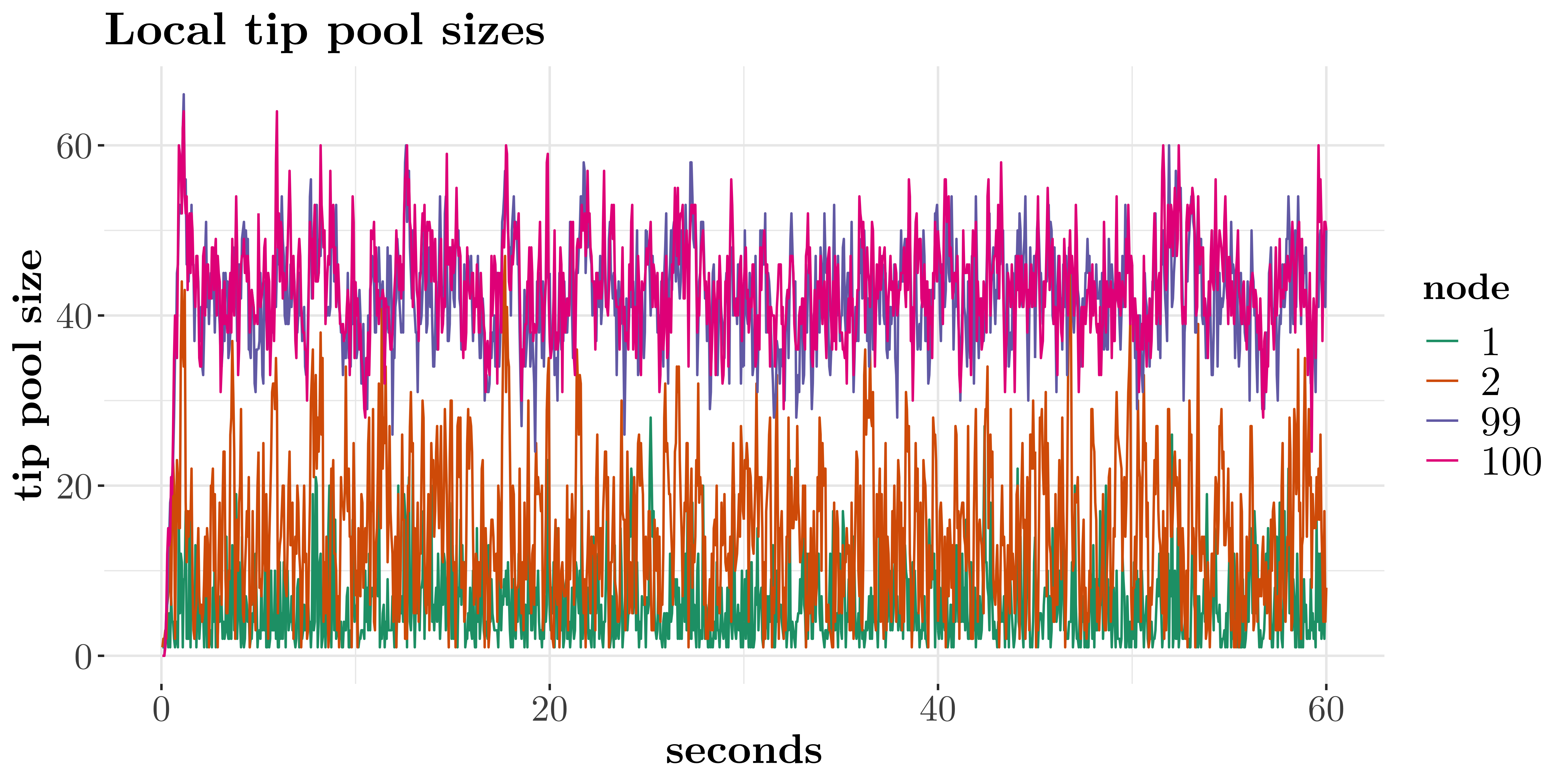
(a) Heterogeneous rates according to Zipf law with $s=1$, BPS of $500$, and random network delay.

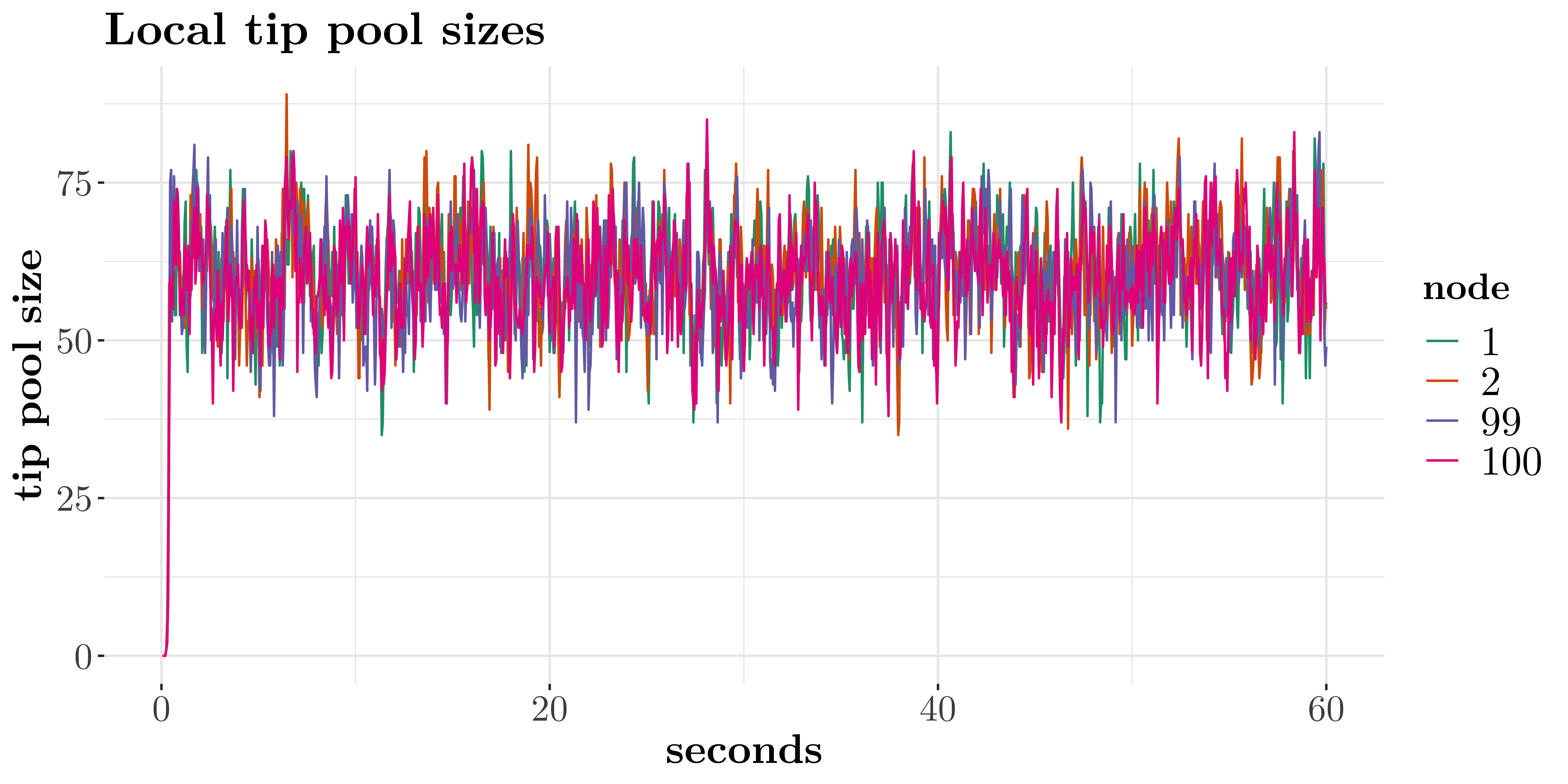
(b) Homogeneous rates according to Zipf law with $s=0$, BPS of $500$, and random network delay.

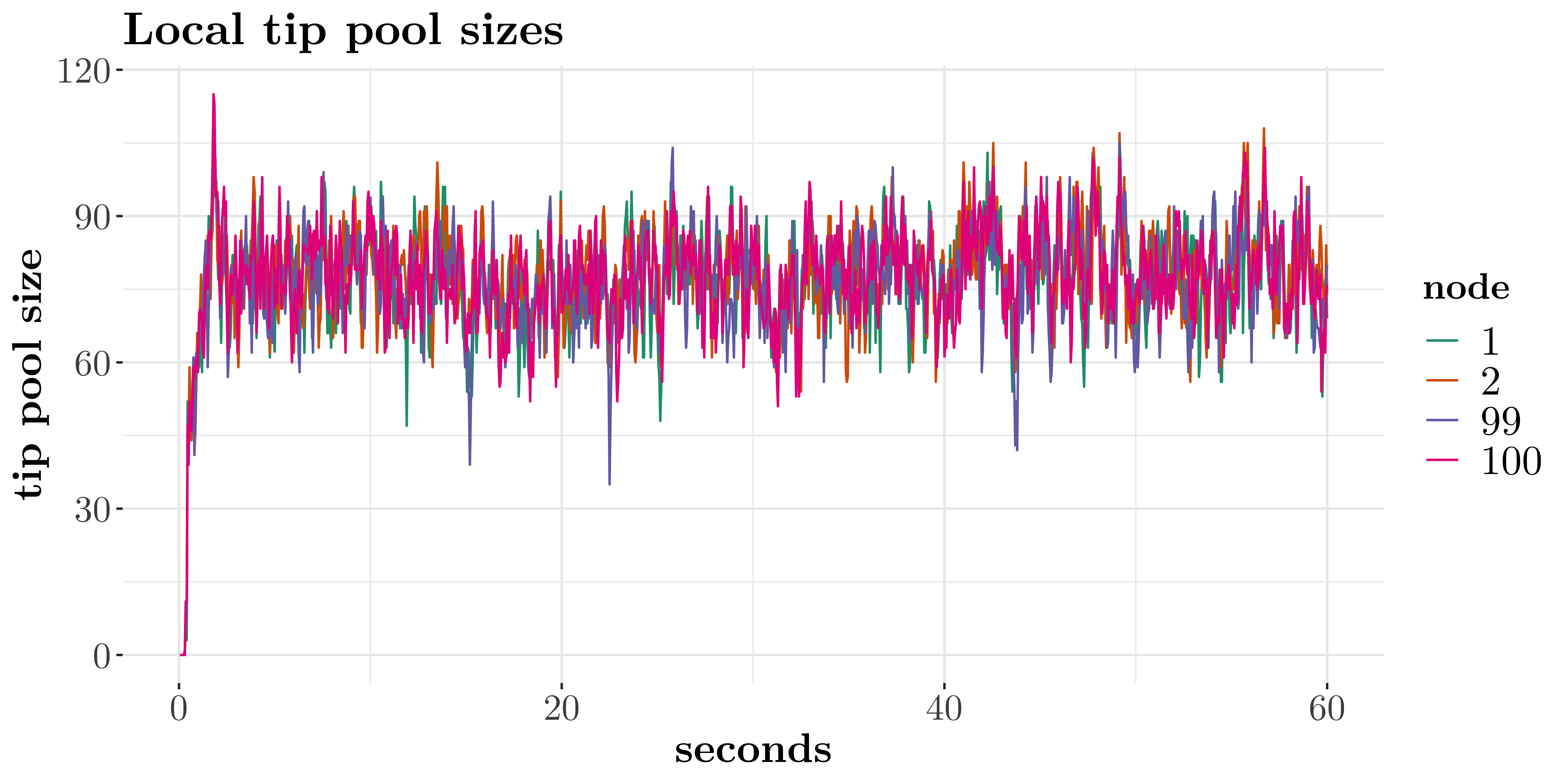
(c) Homogeneous rates according to Zipf law with $s=0$, BPS of $500$, and constant network delay of $100$ms.

Figure 1. Tip pool sizes of the top and bottom nodes with $N=100$ nodes for different scenarios. Randomness in the delay results in smaller tip pool sizes. Heterogeneity in the rates results in more disparate and smaller tip pool sizes.

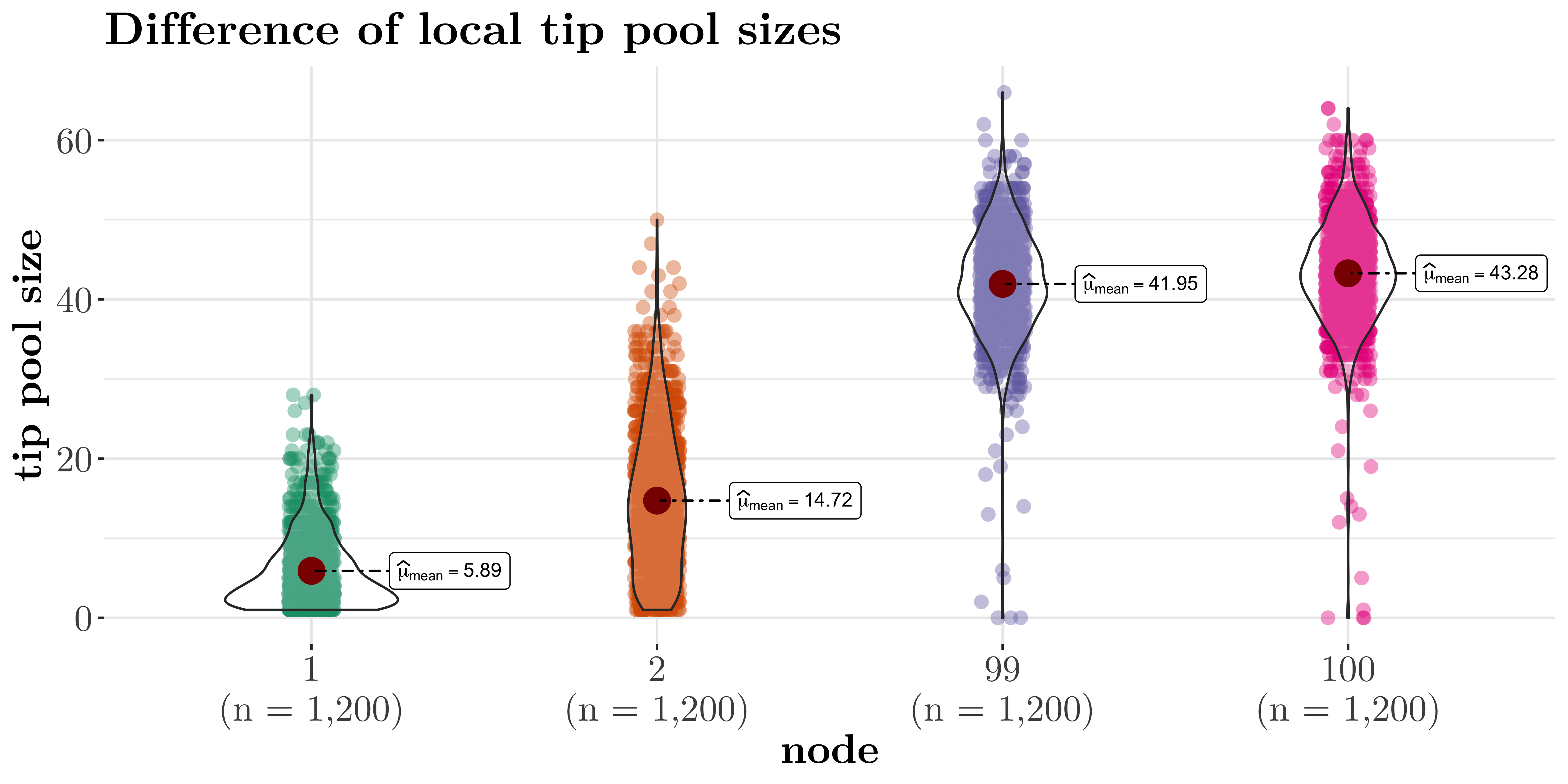
(a) Heterogeneous rates according to Zipf law with $s=1$, BPS of $500$, and random network delay.

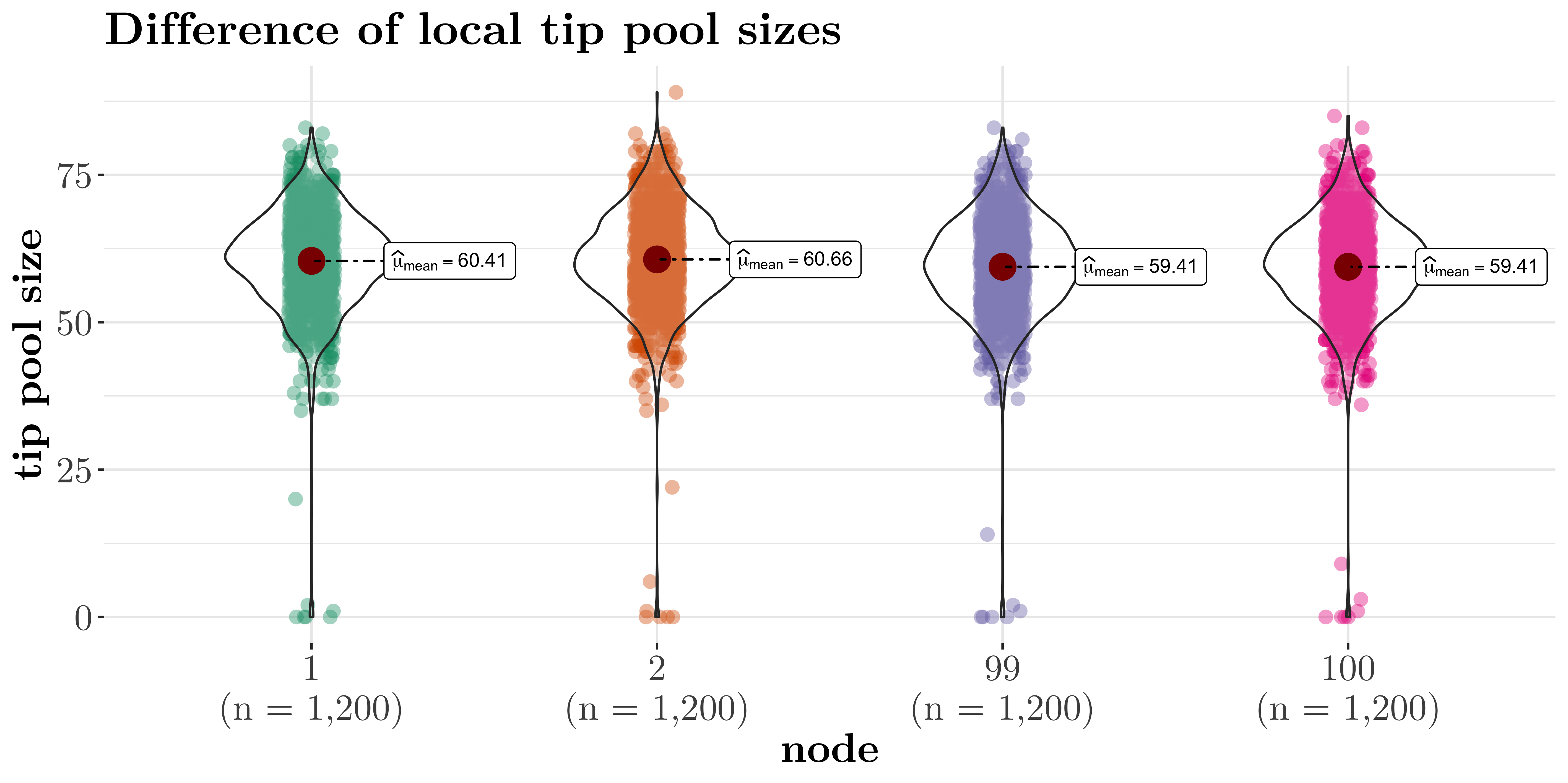
(b) Homogeneous rates according to Zipf law with $s=0$, BPS of $500$, and random network delay.

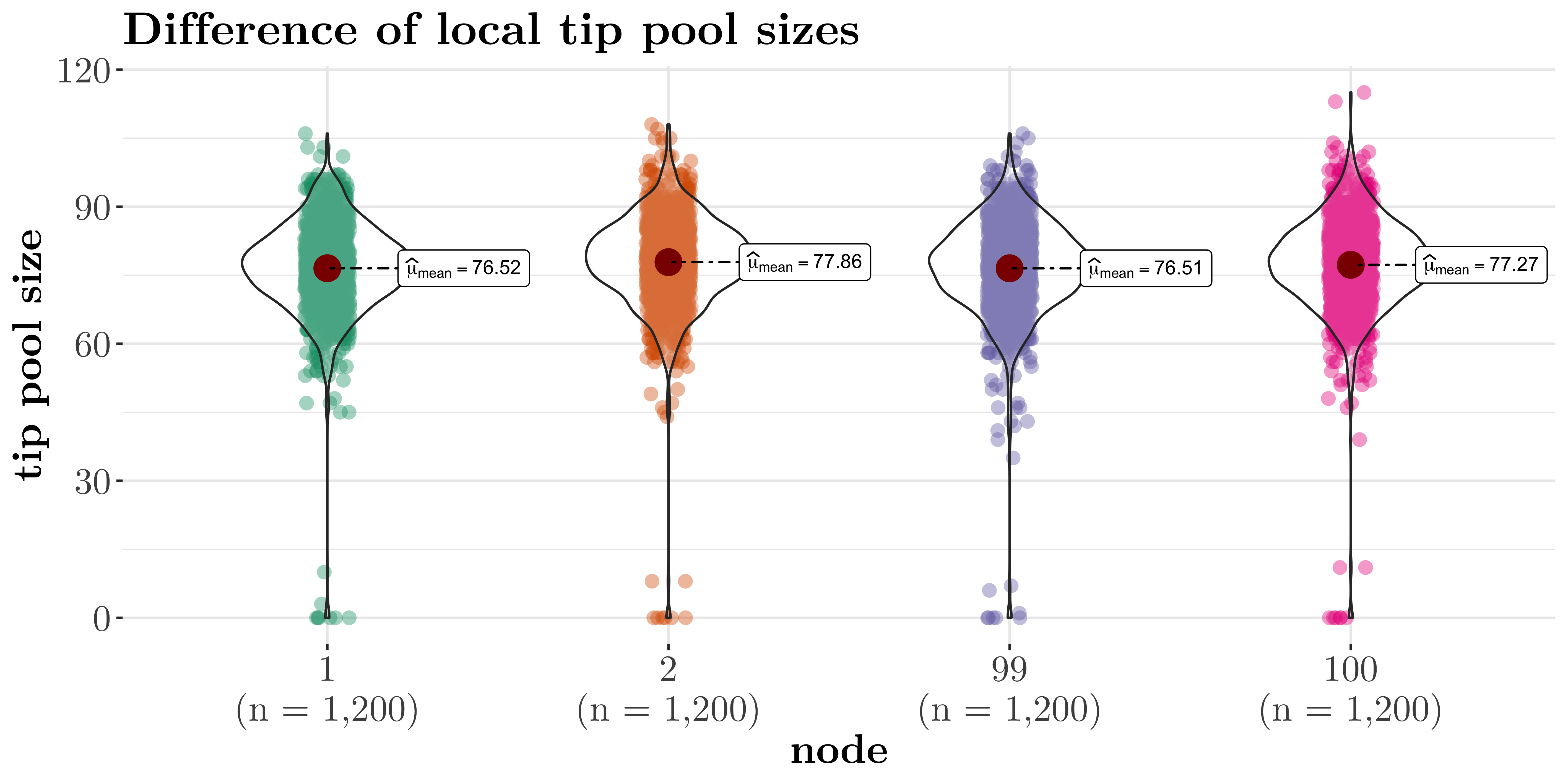
(c) Homogeneous rates according to Zipf law with $s=0$, BPS of $500$, and constant network delay of $100$ms.

Figure 2. Comparison of the local tip pool sizes; $N=100$ nodes, different scenarios.

5. Discussion and extensions

This paper presents a DAG-based distributed ledgers model that considers variable and heterogeneous network delays. It is a continuous time model with random arrivals of new blocks and random communication delays between the nodes. First, we have proven asymptotic negative drift of the tip pool sizes, 3.1, that implies concentration results, Theorem 3.2. A regeneration structure then led to the stationarity and ergodicity of the tip pool sizes, Theorem 3.10. Finally, using Monte-Carlo simulations, we showcase the impact of the rate distribution and the randomness of delays on the evolution of the local tip pool sizes. Let us discuss possible extensions of our work.

Different type of delays: As already mentioned in subsection 1.3, a different type of delay (time to validate a block) has been studied in [31]. One natural way to incorporate such delays is to include an additional mark in the Poisson point process that encodes the block type. The delays of a block then also depend on its type. While our obtained results carry over to this more general situation, understanding how these delays impact the tip pool sizes is more challenging as it requires more quantitative results.

Quantitative results We obtained qualitative results about the stability. For real-world applications, quantitative bounds are essential. The most important measure is the expected tip pool size. Previous results, [20, 31, 6], and our simulations show that the tip pool size depends on the distribution of the delays. Hence, explicit formulas for the expected tip pool size seem currently out of reach. A more feasible approach is to obtain meaningful upper and lower bounds on the tip pool sizes. Moreover, Figures 1 and 2 show the fast convergence to the stationary regime, and it seems achievable to obtain quantitative bounds on this speed of convergence as described in Remark 3.7.

Extreme values and large deviations: In Theorem 3.2, we derived an upper bound on the probability that $X_{k}^{(o)}$ is greater than a given value $L$. Such a result is important from an application perspective because we can quantify the risk that the number of tips is too high at a given instant. The probabilities of deviating from the mean are usually expressed by large deviation results and the distribution of the maximal values by extreme value results. The regeneration structure introduced in Section 3.2 offers an i.i.d. decomposition of the underlying process and, with the exponential moment bounds, strongly suggests the validity of a large deviation principle and an extreme value theorem. We refer to [32] for details on how to obtain a large deviation principle from a regeneration structure and to [2], Chapter IV Section 4, for more details on extreme value theory for regenerative processes.

General arrival point processes: In our model, the assumption of a pure Poisson point process is not necessary, and the results seem to carry over the stationary and ergodic point processes. A more realistic model, for instance, is to consider stationary point processes with minimal distance between the points; so-called hard care point processes.

References

- [1] Lada A. Adamic and B. Huberman. Zipf’s law and the internet. Glottometrics, 3:143–150, 2002.
- [2] Søren Asmussen. Applied Probability and Queues. Springer Publishing Company, Incorporated, New York, 2nd edition, 2003.
- [3] Vivek Bagaria, Sreeram Kannan, David Tse, Giulia Fanti, and Pramod Viswanath. Prism: Deconstructing the blockchain to approach physical limits. In Proceedings of the 2019 ACM SIGSAC Conference on Computer and Communications Security, pages 585–602, 2019.
- [4] Quentin Bramas. The Stability and the Security of the Tangle. working paper or preprint, April 2018.
- [5] Anton Churyumov. Byteball: A decentralized system for storage and transfer of value, 2016.
- [6] A. Cullen, P. Ferraro, C. King, and R. Shorten. Distributed ledger technology for smart mobility: Variable delay models. In 2019 IEEE 58th Conference on Decision and Control (CDC), pages 8447–8452, 2019.
- [7] Philip Daian, Steven Goldfeder, Tyler Kell, Yunqi Li, Xueyuan Zhao, Iddo Bentov, Lorenz Breidenbach, and Ari Juels. Flash boys 2.0: Frontrunning in decentralized exchanges, miner extractable value, and consensus instability. In 2020 IEEE Symposium on Security and Privacy (SP), pages 910–927, 2020.
- [8] George Danezis, Lefteris Kokoris-Kogias, Alberto Sonnino, and Alexander Spiegelman. Narwhal and Tusk: A DAG-Based Mempool and Efficient BFT Consensus. In Proceedings of the Seventeenth European Conference on Computer Systems, EuroSys ’22, page 34–50, New York, NY, USA, 2022. Association for Computing Machinery.
- [9] Alex de Vries and Christian Stoll. Bitcoin’s growing e-waste problem. Resources, Conservation and Recycling, 175:105901, 2021.
- [10] Cynthia Dwork, Nancy Lynch, and Larry Stockmeyer. Consensus in the presence of partial synchrony. J. ACM, 35(2):288–323, apr 1988.
- [11] Pietro Ferraro, Christopher King, and Robert Shorten. Distributed ledger technology for smart cities, the sharing economy, and social compliance. IEEE Access, 6:62728–62746, 2018.
- [12] Pietro Ferraro, Christopher King, and Robert Shorten. Iota-based directed acyclic graphs without orphans. arXiv preprint arXiv:1901.07302, 2018.
- [13] Yossi Gilad, Rotem Hemo, Silvio Micali, Georgios Vlachos, and Nickolai Zeldovich. Algorand: Scaling byzantine agreements for cryptocurrencies. In Proceedings of the 26th symposium on operating systems principles, pages 51–68, 2017.
- [14] Adam Gągol, Damian Leśniak, Damian Straszak, and Michał Świętek. Aleph: Efficient atomic broadcast in asynchronous networks with byzantine nodes. In Proceedings of the 1st ACM Conference on Advances in Financial Technologies, pages 214–228, 2019.
- [15] Bruce Hajek. Hitting-time and occupation-time bounds implied by drift analysis with applications. Advances in Applied Probability, 14(3):502–525, 1982.
- [16] Bruce Hajek. Random Processes for Engineers. Cambridge University Press, Cambridge, 2015.
- [17] IOTA Foundation. Multiverse Simulation. https://github.com/iotaledger/multiverse-simulation, 2022. [Online; accessed 15/11 2022].
- [18] Charles I. Jones. Pareto and Piketty: The Macroeconomics of Top Income and Wealth Inequality. Journal of Economic Perspectives, 29(1):29–46, February 2015.
- [19] E. Kamrani, H.R. Momeni, and A.R. Sharafat. Modeling internet delay dynamics for teleoperation. In Proceedings of 2005 IEEE Conference on Control Applications, 2005. CCA 2005., pages 1528–1533, 2005.
- [20] Navdeep Kumar, Alexandre Reiffers-Masson, Isabel Amigo, and Santiago Ruano Rincón. The effect of network delays on distributed ledgers based on direct acyclic graphs: A mathematical model. Available at SSRN 4253421, 2022.
- [21] Bartosz Kusmierz, William Sanders, Andreas Penzkofer, Angelo Capossele, and Alon Gal. Properties of the tangle for uniform random and random walk tip selection. In 2019 IEEE International Conference on Blockchain (Blockchain), pages 228–236. IEEE, 2019.
- [22] Wentian Li. Zipf’s law everywhere. Glottometrics, 5:14–21, 2002.
- [23] Yixin Li, Bin Cao, Mugen Peng, Long Zhang, Lei Zhang, Daquan Feng, and Jihong Yu. Direct acyclic graph-based ledger for internet of things: performance and security analysis. IEEE/ACM Transactions on Networking, 28(4):1643–1656, 2020.
- [24] Bing-Yang Lin, Daria Dziubałtowska, Piotr Macek, Andreas Penzkofer, and Sebastian Müller. Robustness of the Tangle 2.0 Consensus, 2022.
- [25] Igor Makarov and Antoinette Schoar. Blockchain analysis of the bitcoin market. Working Paper 29396, National Bureau of Economic Research, October 2021.
- [26] Sebastian Müller, Andreas Penzkofer, Nikita Polyanskii, Jonas Theis, William Sanders, and Hans Moog. Tangle 2.0 Leaderless Nakamoto Consensus on the Heaviest DAG. IEEE Access, 10:105807–105842, 2022.
- [27] Satoshi Nakamoto. Bitcoin: A peer-to-peer electronic cash system, 2008.
- [28] Seongjoon Park, Seounghwan Oh, and Hwangnam Kim. Performance analysis of dag-based cryptocurrency. In 2019 IEEE International Conference on Communications workshops (ICC workshops), pages 1–6. IEEE, 2019.
- [29] Indrajeet Patil. Visualizations with statistical details: The ’ggstatsplot’ approach. Journal of Open Source Software, 6(61):3167, 2021.
- [30] Robin Pemantle and Jeffrey S. Rosenthal. Moment conditions for a sequence with negative drift to be uniformly bounded in Lr. Stochastic Processes and their Applications, 82(1):143–155, 1999.
- [31] Andreas Penzkofer, Olivia Saa, and Daria Dziubałtowska. Impact of delay classes on the data structure in iota. In Data Privacy Management, Cryptocurrencies and Blockchain Technology, pages 289–300. Springer, 2021.
- [32] Jonathon Peterson and Ofer Zeitouni. On the annealed large deviation rate function for a multi-dimensional random walk in random environment. arXiv: Probability, 2008.
- [33] Serguei Popov. The Tangle, 2015.
- [34] Serguei Popov, Hans Moog, Darcy Camargo, Angelo Capossele, Vassil Dimitrov, Alon Gal, Andrew Greve, Bartosz Kusmierz, Sebastian Mueller, Andreas Penzkofer, Olivia Saa, William Sanders, Luigi Vigneri, Wolfgang Welz, and Vidal Attias. The Coordicide. 2020.
- [35] David M. W. Powers. Applications and explanations of Zipf’s law. In New Methods in Language Processing and Computational Natural Language Learning, 1998.
- [36] David Rosenthal. EE380 Talk, 2022.
- [37] Yonatan Sompolinsky, Yoad Lewenberg, and Aviv Zohar. Spectre: A fast and scalable cryptocurrency protocol. Cryptology ePrint Archive, Report 2016/1159, 2016.
- [38] Yonatan Sompolinsky, Shai Wyborski, and Aviv Zohar. Phantom and ghostdag: A scalable generalization of nakamoto consensus. Cryptology ePrint Archive, Report 2018/104, 2018.
- [39] Yonatan Sompolinsky and Aviv Zohar. Secure high-rate transaction processing in bitcoin. In Rainer Böhme and Tatsuaki Okamoto, editors, Financial Cryptography and Data Security, pages 507–527, Berlin, Heidelberg, 2015. Springer Berlin Heidelberg.
- [40] Duncan J Watts and Steven H Strogatz. Collective dynamics of ‘small-world’networks. nature, 393(6684):440–442, 1998.
- [41] Manuel Zander, Tom Waite, and Dominik Harz. Dagsim: Simulation of dag-based distributed ledger protocols. ACM SIGMETRICS Performance Evaluation Review, 46(3):118–121, 2019.