Fundamental solutions of an extended hydrodynamic model in two dimensions: Derivation, theory, and applications

Abstract

The inability of the Navier–Stokes–Fourier equations to capture rarefaction effects motivates us to adopt the extended hydrodynamic equations. In the present work, a hydrodynamic model, which consists of the conservation laws closed with the recently propounded coupled constitutive relations (CCR), is utilized. This model is referred to as the CCR model and is adequate for describing moderately rarefied gas flows. A numerical framework based on the method of fundamental solutions is developed to solve the CCR model for rarefied gas flow problems in quasi two dimensions. To this end, the fundamental solutions of the linearized CCR model are derived in two dimensions. The significance of deriving the two-dimensional fundamental solutions is that they cannot be deduced from their three-dimensional counterparts that do exist in literature. As applications, the developed numerical framework based on the derived fundamental solutions is used to simulate (i) a rarefied gas flow between two coaxial cylinders with evaporating walls and (ii) a temperature-driven rarefied gas flow between two non-coaxial cylinders. The results for both problems have been validated against those obtained with the other classical approaches. Through this, it is shown that the method of fundamental solutions is an efficient tool for addressing quasi two-dimensional multiphase microscale gas flow problems at a low computational cost. Moreover, the findings also show that the CCR model solved with the method of fundamental solutions is able to describe rarefaction effects, like transpiration flows and thermal stress, generally well.

I Introduction

The study of rarefied gases covers numerous applications, including flows caused by evaporation and condensation, upper-atmospheric dynamics, modeling of airborne particles, the reflective and reactive properties of gases interacting with solid and liquid surfaces and so on. Rarefied gas flows are characterized by a dimensionless parameter, the Knudsen number ($\mathrm{Kn}$), which is the ratio of the mean free path $\lambda$ of the gas and a characteristic length scale $L$ in the problem. For very small values of the Knudsen number ($\mathrm{Kn}\lesssim 0.01$), the classical continuum theories, namely the Euler and Navier–Stokes–Fourier (NSF) equations, are quite effective in capturing rarefaction effects but they fall short of doing so when the Knudsen number is not very small. Although the NSF equations fail to capture several non-equilibrium phenomena (like non-homogeneity in pressure profile and unusual temperature dip in the Poiseuille flow (Ohwada, Sone, and Aoki, 1989; Taheri, Torrilhon, and Struchtrup, 2009; Rana et al., 2016), heat flux direction opposite to the temperature gradient or the cross effects where heat flows from a low-temperature region to a high-temperature region (Struchtrup and Torrilhon, 2008; Mohammadzadeh, Rana, and Struchtrup, 2015; Rana, Torrilhon, and Struchtrup, 2013)), yet, by exploiting the coupling among the thermodynamic forces and fluxes to form a closed system, the range of applicability of the new equations is enhanced in comparison to the NSF equations. A model that exploits the coupling among the thermodynamic forces and fluxes to yield an improved set of constitutive relations for the stress and heat flux appearing in the conservation laws has recently been propounded by Rana et al. [Rana, Gupta, and Struchtrup, 2018]. The constitutive relations for the stress and heat flux obtained in this model are coupled through a coupling coefficient; hence they are referred to as the coupled constitutive relations (CCR), and the model wherefore is referred to as the CCR model. In the linearized and steady state, the CCR model reduces to the linearized Grad 13-moment (G13) equations Grad (1949) in the steady state as a special case, and on taking the coupling coefficient as zero, the CCR model reduces to the original NSF equations. Owing to its simplicity and viable features, the CCR model has been applied successfully to some problems pertaining to rarefied gas flows Rana et al. (2021); Modi and Rana (2022). Although, there do exist other models, such as the regularized 13-moment (R13) equations Struchtrup and Torrilhon (2003); Struchtrup (2005), the regularized 26-moment (R26) equations Gu and Emerson (2009), etc., that can describe rarefied gas flows somewhat more accurately than the CCR model, especially for flows at moderate Knudsen numbers, we shall use the CCR model due to its simplicity in this work.

In this paper, we shall focus our attention to exploring rarefied gas flow problems in (quasi) two dimensions (2D). The reason for this is twofold: firstly, for a symmetric uniform flow in three dimensions (3D), it is sufficient to study the problem in 2D, thanks to the symmetry along the transverse direction, and secondly, there are some intriguing problems in 2D that do not arise in 3D, such as Stokes’ paradox (Lamb, 1932), which states the non-existence of the steady-state solution to Stokes’ equation in 2D. Furthermore, we shall investigate the problems numerically using a truly meshless numerical technique introduced by Kupradze and Aleksidze(Kupradze and Aleksidze, 1964) known as the method of fundamental solutions (MFS).

The MFS is a meshfree method that yields remarkably good results with a significantly less computational effort if the singularity points (also referred to as the source points) are placed at proper locations. The meshfree feature of the MFS is especially useful in the situations wherein changes in the shape of the domain are needed, e.g., in shape optimization and inverse problems. This is because the MFS does not require creating a mesh over the entire domain, which itself could be a very time-consuming and computationally-expensive task depending on the complexity of the domain. In the MFS, an approximate solution of a (linear) boundary value problem is expressed as a superposition of Green’s functions, referred to as the fundamental solutions, and the boundary conditions are satisfied at several locations on the boundary, referred to as the boundary nodes or collocation points, aiming to determine the unknown coefficients in the linear combination. Apart from being time-efficient due to reduced spatial dimension in boundary discretization, the quality of being free from integrals makes the MFS peerless among other meshfree methods (such as the boundary element method (Brebbia and Dominguez, 1994), finite point method (Oñate et al., 1996), diffuse element method (Nayroles, Touzot, and Villon, 1992), element-free Galerkin method (Belytschko, Lu, and Gu, 1994)) that involve complex integrals. The MFS has proven to be an efficient executable numerical scheme in various areas, such as thermoelasticity, electromagnetics, electrostatics, wave scattering, inverse problems and fluid flow problems; see, e.g. Refs. [Liu, Fan, and Šarler, 2021; Berger and Karageorghis, 2001; Fairweather, Karageorghis, and Martin, 2003; Karageorghis, Lesnic, and Marin, 2011; Young et al., 2006; Lockerby and Collyer, 2016]. Moreover, the MFS is also suitable for the analysis of problems involving shape optimization, moving boundary and unknown boundary (Fam and Rashed, 2002; Young et al., 2006; Chen, Karageorghis, and Smyrlis, 2008; Shigeta, Young, and Liu, 2012; Alves, 2009), since the problems of modeling and satisfying boundary conditions are relatively simple for them. All these advantages make the application of the MFS to the CCR model evidently favorable.

Several researchers have employed the MFS to solve the Helmholtz-, harmonic- and biharmonic-type boundary value problems in 2D as well as in 3D, see e.g., Refs. [Poullikkas, Karageorghis, and Georgiou, 1998; Marin and Lesnic, 2005]. The MFS works as a good numerical strategy if the fundamental solutions to the problem are predefined. In the past few years, there has been a surge of interest in employing the MFS to various models for rarefied gas flows, for instance to the NSF, G13, R13 and CCR models (Lockerby and Collyer, 2016; Claydon et al., 2017; Rana et al., 2021), because the predefined fundamental solutions of the well-known equations, such as the Laplace, Helmholtz and biharmonic equations, can be exploited to determine the fundamental solutions for the NSF, G13, R13 and CCR models. Nevertheless, all the works on the MFS for rarefied gas flows have investigated the problems in 3D only. But, for quasi two-dimensional flow problems, it is not really necessary to solve the full three-dimensional problem as the flow profiles obtained in a cross section perpendicular to the transverse direction remain the same in any cross section perpendicular to the transverse direction. Thus, a quasi two-dimensional study of a full three-dimensional problem (where one dimension in the problem is much larger than the other two) reduces the computational cost of any numerical technique exceedingly. Interestingly, in the case the MFS, the two-dimensional fundamental solutions for a model cannot be deduced directly from its three-dimensional counterpart due to the fact that the associated Green’s functions are entirely different in 2D and 3D. Therefore the main objectives of the paper are (i) to determine the two-dimensional fundamental solutions of the linearized CCR model and (ii) to implement the determined fundamental solutions in a numerical framework. To gauge the accuracy of the developed numerical framework, the obtained numerical results are also validated against those obtained with other models for a few problems existing in the literature. We pick two internal-flow problems from Refs. [Onishi, 1977; Aoki, Sone, and Yano, 1989] that have been investigated in these references with the linearized Bhatnagar–Gross–Krook (BGK) model (Bhatnagar, Gross, and Krook, 1954) [also referred to as the Boltzmann–Krook–Welander (BKW) kinetic model by some authors Onishi (1977); Aoki, Sone, and Yano (1989); Sone (2007)]. In the first problem, the evaporation and condensation of a mildly rarefied vapor confined between two coaxial cylinders is studied while in the second problem, a temperature-driven rarefied gas flow between two non-coaxial cylinders is investigated.

In the MFS, positioning of the singularity points has been a widely-discussed issue in order to achieve accurate results (Alves, 2009; Chen, Karageorghis, and Li, 2016; Wang, Liu, and Qu, 2018; Cheng and Hong, 2020) due to the fact that the linear system resulting from the MFS can have an ill-conditioned coefficient matrix (Alves, 2009), and there is a trade-off between the accuracy and well conditioning. For meshfree methods, including the MFS, Alves [Alves, 2009] states, “In these methods a sort of uncertainty principle occurs—we cannot get both accurate results and good conditioning—one of the two is lost.” In this paper, we also demonstrate a method to determine an appropriate location of singularity points for obtaining the solutions of a desired accuracy using an approach based on the effective condition number as discussed in Refs. [Drombosky, Meyer, and Ling, 2009; Chen et al., 2023; Wong and Ling, 2011].

The remainder of the paper is structured as follows. The linearized CCR model and the generalized boundary conditions associated with it are outlined in Sec. II. The two-dimensional fundamental solutions for the CCR model are determined in Sec. III. The technique to apply the MFS by forming a system of equations for any arbitrary geometry is discussed in Sec. IV. The implementation of the MFS along with its validation (i) for the problem of a vapor flow between two coaxial cylinders is demonstrated in Sec. V and (ii) for the problem of a temperature-driven rarefied gas flow between two non-coaxial cylinders is discussed in Sec. VI. The location of singularities based on the effective condition number approach is examined in Sec. VII. The paper ends with conclusions and outlook in Sec. VIII.

II The linearized CCR model and boundary conditions

The CCR model consists of the conservation laws—the balance equations for the mass, momentum and energy—closed with the constitutive relations for the stress and heat flux, which are coupled with each other through a coupling coefficient. The full details of the CCR model can be found in Ref. [Rana, Gupta, and Struchtrup, 2018]. In this work, we require them in the linearized form. To this end, we convert the mass, momentum and energy balance equations and the coupled constitutive relations into a linear-dimensionless form by assuming small perturbations in flow fields from their respective equilibrium values. The velocity, stress and heat flux in the equilibrium state vanish whereas the density and temperature in the equilibrium state are constants $\tilde{\rho}_{0}$ and $\tilde{T}_{0}$, respectively. The dimensionless perturbations in the density $\tilde{\rho}$ and temperature $\tilde{T}$ from their values in the equilibrium are given by

$$\rho=\frac{\tilde{\rho}-\tilde{\rho}_{0}}{\tilde{\rho}_{0}}\quad\text{and}\quad T=\frac{\tilde{T}-\tilde{T}_{0}}{\tilde{T}_{0}},$$ (1)

respectively. Similarly, the dimensionless perturbations in the velocity $\tilde{\bm{v}}$, stress tensor $\tilde{\bm{\sigma}}$ and heat flux $\tilde{\bm{q}}$ from their values in the equilibrium are given by

$$\bm{v}=\frac{\tilde{\bm{v}}}{\sqrt{\tilde{\theta}_{0}}},\quad\bm{\sigma}=\frac{\tilde{\bm{\sigma}}}{\tilde{\rho}_{0}\tilde{\theta}_{0}}\quad\text{and}\quad\bm{q}=\frac{\tilde{\bm{q}}}{\tilde{\rho}_{0}(\tilde{\theta}_{0})^{3/2}},$$ (2)

respectively, where $\tilde{\theta}_{0}=\tilde{R}\tilde{T_{0}}$ with $\tilde{R}$ being the gas constant. The linearized equation of state $p\approx\rho+T$ gives the dimensionless perturbation in the pressure from its equilibrium value $\tilde{p}_{0}=\tilde{\rho}_{0}\tilde{\theta}_{0}$. For the sake of simplicity, the field variables with tilde are the quantities with dimensions while those without tilde are the dimensionless quantities throughout the paper.

Considering $\tilde{L}$ to be the characteristic length scale, the dimensionless position vector is $\bm{r}=\tilde{\bm{r}}/\tilde{L}$. Inserting these dimensionless variables into the CCR model Rana, Gupta, and Struchtrup (2018) and dropping all nonlinear terms in the perturbed variables, one readily obtains the linear-dimensionless CCR model. Here, we present them directly. The linear-dimensionless mass, momentum and energy balance equations in the steady state read

$$\bm{\nabla}\cdot\bm{v}=0,$$ (3)

$$\bm{\nabla}p+\bm{\nabla}\cdot\bm{\sigma}=\bm{0},$$ (4)

$$\bm{\nabla}\cdot\bm{q}=0,$$ (5)

and, to close the system (3)–(5), we adopt the linearized coupled constitutive relations(Rana, Gupta, and Struchtrup, 2018)

$$\bm{\sigma} =-2\mathrm{Kn}\overline{\bm{\nabla}\bm{v}}-2\alpha_{0}\mathrm{Kn}\overline{\bm{\nabla}\bm{q}},$$ (6)

$$\bm{q} =-\frac{c_{p}\mathrm{Kn}}{\mathrm{Pr}}(\bm{\nabla}T+\alpha_{0}\bm{\nabla}\cdot\bm{\sigma}),$$ (7)

where $\alpha_{0}$ is the coupling coefficient through which constitutive relations (6) and (7) are coupled; $c_{p}=\tilde{c}_{p}/\tilde{R}$ with $\tilde{c}_{p}$ being the specific heat capacity of the gas at a constant pressure; and

$$\mathrm{Pr}=\frac{\tilde{c}_{p}\tilde{\mu}_{0}}{\tilde{\kappa}_{0}}\quad\text{and}\quad\mathrm{Kn}=\frac{\tilde{\mu}_{0}}{\tilde{\rho}_{0}\sqrt{\tilde{\theta}_{0}}\tilde{L}}$$ (8)

are the Prandtl number and Knudsen number, respectively, with $\tilde{\mu}_{0}$ and $\tilde{\kappa}_{0}$ being the viscosity and thermal conductivity at the equilibrium state. The quantities $\overline{\bm{\nabla}\bm{v}}$ and $\overline{\bm{\nabla}\bm{q}}$ in (6) are the symmetric-tracefree parts of the tensors $\bm{\nabla}\bm{v}$ and $\bm{\nabla}\bm{q}$, respectively. For a $d$-dimensional vector $\bm{\psi}$, the symmetric-tracefree part of the tensor $\bm{\nabla}\bm{\psi}$ is defined as Gupta (2020)

$$\overline{\bm{\nabla}\bm{\psi}} =\frac{1}{2}\Big{[}{\bm{\nabla}\bm{\psi}}+(\bm{\nabla}\bm{\psi})^{\mathsf{T}}\Big{]}-\frac{1}{d}(\bm{\nabla}\cdot\bm{\psi})\bm{I},$$ (9)

where $\bm{I}$ is the identity tensor in $d$ dimensions. For three-dimensional and quasi two-dimensional problems, $d=3$. Furthermore, the dimensionless specific heat of a gas at a constant pressure is $c_{p}=(5+\mathsf{n})/2$, where $\mathsf{n}$ is a positive number that accounts for the internal degrees of freedom in a polyatomic gas. For monatomic gases, there is no rotational degree of freedom; consequently, $\mathsf{n}=0$ and $c_{p}=5/2$ for monatomic gases. We shall only deal with monatomic gases in this paper, and hence $c_{p}=5/2$ throughout this paper. Equations (3)–(5) closed with (6) and (7) are referred to as the linearized CCR model. For $\alpha_{0}=0$, the linearized CCR model reduces to the linearized NSF equations and for $\alpha_{0}=2/5$, the steady-state linearized CCR model reduces to the steady-state linearized G13 equations. The parameter $\alpha_{0}$ in the case of the CCR model is taken as $0.3197$, the value of $\alpha_{0}$ for hard sphere molecules Rana, Gupta, and Struchtrup (2018), throughout this paper. Since we shall be comparing the results obtained in the present work with those obtained with the BGK model, for which the Prandtl number is unity Struchtrup (2005), $\mathrm{Pr}=1$ throughout this paper.

For quasi two-dimensional flows, let us say in the $x_{1}x_{2}$-plane, the field variables do not change in the direction perpendicular to the plane of the flow, i.e. they do not change along the $x_{3}$-direction. As a result, the CCR model [Eqs. (3)–(7)] for a quasi two-dimensional flow in the $x_{1}x_{2}$-plane reduces to

$$\frac{\partial v_{i}}{\partial x_{i}} =0,$$ (10)

$$\frac{\partial p}{\partial x_{i}}+\frac{\partial\sigma_{ij}}{\partial x_{j}} =0,$$ (11)

$$\frac{\partial q_{i}}{\partial x_{i}} =0,$$ (12)

$$\sigma_{ij}= -2\mathrm{Kn}\left[\frac{1}{2}\left(\frac{\partial v_{i}}{\partial x_{j}}+\frac{\partial v_{j}}{\partial x_{i}}\right)-\frac{1}{3}\delta_{ij}\frac{\partial v_{\ell}}{\partial x_{\ell}}\right]$$

$$-2\alpha_{0}\mathrm{Kn}\left[\frac{1}{2}\left(\frac{\partial q_{i}}{\partial x_{j}}+\frac{\partial q_{j}}{\partial x_{i}}\right)-\frac{1}{3}\delta_{ij}\frac{\partial q_{\ell}}{\partial x_{\ell}}\right],$$ (13)

$$q_{i}= -\frac{c_{p}\mathrm{Kn}}{\mathrm{Pr}}\left(\frac{\partial T}{\partial x_{i}}+\alpha_{0}\frac{\partial\sigma_{ij}}{\partial x_{j}}\right),$$ (14)

where the indices $i,j$ and $\ell$ can take the values $1$ and $2$ only, $\delta_{ij}$ is the Kronecker delta and the Einstein summation applies over the repeated indices in a term. It may be noted that Eq. (11) represents two equations: for $i=1$ the momentum balance equation in the $x_{1}$-direction and for $i=2$ the momentum balance equation in the $x_{2}$-direction, and that the momentum balance equation in the $x_{3}$-direction is identically satisfied. It is also worthwhile noting that $\sigma_{11}+\sigma_{22}=0$ in view of Eqs. (10) and (12), which is consistent with the fact that the stress tensor $\bm{\sigma}$ is tracefree because $\sigma_{33}=0$ for quasi two-dimensional flows in the $x_{1}x_{2}$-plane. Thus, the CCR model for a quasi two-dimensional flow in the $x_{1}x_{2}$-plane [Eqs. (10) and (14)] essentially consists of the unknown field variables $v_{1},v_{2},p,T,\sigma_{11},\sigma_{12},q_{1},q_{2}$. Therefore, the fundamental solutions of the CCR model for a quasi two-dimensional flow—determined in the next section—will be referred to as the two-dimensional fundamental solutions of the CCR model or the fundamental solutions of the CCR model in 2D.

The thermodynamically-consistent boundary conditions complementing the linear CCR model have been derived in Ref. [Rana et al., 2021]. For a three-dimensional problem, the boundary conditions complementing the linear CCR model are given in Eqs. $(4.2a)$, $(4.2b)$, $(4.3a)$ and $(4.3b)$ of Ref. [Rana et al., 2021]. Equations $(4.2a)$ and $(4.2b)$ of Ref. [Rana et al., 2021] are the boundary conditions on the normal components of the mass and heat fluxes, respectively, while Eqs. $(4.3a)$ and $(4.3b)$ of Ref. [Rana et al., 2021] are the boundary conditions on the shear stress—two conditions due to two tangential directions in 3D. Since for a quasi two-dimensional flow in the $x_{1}x_{2}$-plane, the wall normal direction and one tangential direction are in the $x_{1}x_{2}$-plane while the other tangential direction is along the $x_{3}$-direction, boundary condition $(4.3b)$ of Ref. [Rana et al., 2021] is irrelevant in the present work and the superscript ‘$(1)$’ can be dropped from the unit tangent vector $\bm{t}^{(1)}$ in $(4.3a)$ of Ref. [Rana et al., 2021] for simplicity. Thus, the linear-dimensionless boundary conditions complementing the linearized CCR model for a quasi two-dimensional flow read Rana et al. (2021)

$$(\bm{v}-\bm{v}^{I})\cdot\bm{n}= -\eta_{11}(p-p_{\mathrm{sat}}+\bm{n}\cdot\bm{\sigma}\cdot\bm{n})$$

$$+\eta_{12}(T-T^{I}+\alpha_{0}\bm{n}\cdot\bm{\sigma}\cdot\bm{n}),$$ (15)

$$\bm{q}\cdot\bm{n}= \medspace\eta_{12}(p-p_{\mathrm{sat}}+\bm{n}\cdot\bm{\sigma}\cdot\bm{n})$$

$$-(\eta_{22}+2\tau_{0})(T-T^{I}+\alpha_{0}\bm{n}\cdot\bm{\sigma}\cdot\bm{n}),$$ (16)

$$\bm{t}\cdot\bm{\sigma}\cdot\bm{n}= -\varsigma(\bm{v}-\bm{v}^{I}+\alpha_{0}\bm{q})\cdot\bm{t},$$ (17)

where $\bm{n}$ and $\bm{t}$ are the unit normal and tangent vectors, respectively. In boundary conditions (II)–(17), $\eta_{ij}$’s, for $i,j\in\{1,2\}$ are the Onsager reciprocity coefficients, which from Sone’s asymptotic kinetic theory (Sone, 2007) turn out to be

$$\left.\begin{aligned} \eta_{11}&=0.9134\sqrt{\frac{2}{\pi}}\frac{\vartheta}{2-\vartheta},\\ \eta_{12}&=0.3915\sqrt{\frac{2}{\pi}}\frac{\vartheta}{2-\vartheta},\\ \eta_{22}&=0.1678\sqrt{\frac{2}{\pi}}\frac{\vartheta}{2-\vartheta}\end{aligned}\right\}$$ (18)

under the assumption of the accommodation coefficient being unity (which also holds true for the diffuse reflection boundary condition). The parameter $\vartheta$ in the above coefficients is the evaporation/condensation coefficient. For canonical boundaries and phase-change boundaries, $\vartheta=0$ and $1$, respectively, are the largely accepted values of $\vartheta$ in the literature. The temperature-jump and velocity-slip coefficients are given by Rana et al. (2021)

$$\tau_{0}=0.8503\sqrt{\frac{2}{\pi}}\quad\text{and}\quad\varsigma=0.8798\sqrt{\frac{2}{\pi}},$$ (19)

respectively. Furthermore, $\bm{v}^{I}$, $T^{I}$ and $p_{\mathrm{sat}}$ in boundary conditions (II)–(17) represent the velocity, temperature and saturation pressure at the interface. It is important to note that the coefficients $\alpha_{0}$ in boundary conditions (II)–(17) are actually the fitting parameters and could be different from the coupling coefficient $\alpha_{0}$. Moreover, the coefficient $\alpha_{0}$ in each of boundary conditions (II)–(17) could also be different from each other. The only reason that the coefficients $\alpha_{0}$ in boundary conditions (II)–(17) have been taken as the same as the coupling coefficient in the CCR model because the boundary conditions obtained in this way are thermodynamically consistent Rana, Gupta, and Struchtrup (2018).

III Derivation of the fundamental solutions of the CCR model

The fundamental solutions of the CCR model in 3D have already been derived in Ref. [Rana et al., 2021]. However, as mentioned in Sec. I, the fundamental solutions of a model in 2D and 3D are independent of each other because the inherent Green’s functions are independent of each other in 2D and 3D; consequently, the two-dimensional fundamental solution of a model cannot be determined from its three-dimensional counterpart in general. Therefore, we derive the fundamental solutions of the CCR model in 2D from scratch in this section. To this end, we add a Dirac delta forcing term of strength $f_{i}$ ($i\in\{1,2\}$) on the right-hand side of the momentum balance equation to represent a (vector) point force, and a point heat source of strength $g$ on the right-hand side of the energy balance equation. Furthermore, to deal with phase-change effects at the liquid-vapor interface, a point mass source of strength $h$ is also added on the right-hand side of the mass balance equation. For determining the fundamental solutions of a system of partial differential equations, it is customary to consider only one point source at a time and then to superimpose the solutions obtained by taking each point source at a time in order to incorporate the effects of all point sources; see, e.g., Refs. [Lockerby and Collyer, 2016; Rana et al., 2021]. Nevertheless, we take all three point sources $\bm{f}\equiv(f_{1},f_{2})^{\mathsf{T}}$, $g$ and $h$ simultaneously and solve the resulting system of equations altogether. We have verified—although not shown here for brevity—that this procedure also yields exactly the same solution as that obtained by superimposing the solutions obtained by solving the systems separately with one point source at a time.

To determine the fundamental solutions of the CCR model in 2D, the mass, momentum and energy balance equations (10)–(12) are written with the point source terms on their right-hand sides. These equations read

$$\frac{\partial v_{i}}{\partial x_{i}} =h\,\delta(\bm{r}),$$ (20)

$$\frac{\partial p}{\partial x_{i}}+\frac{\partial\sigma_{ij}}{\partial x_{j}} =f_{i}\,\delta(\bm{r}),$$ (21)

$$\frac{\partial q_{i}}{\partial x_{i}} =g\,\delta(\bm{r}),$$ (22)

where $\bm{r}=(x_{1},x_{2})^{\mathsf{T}}$. Equations (20)–(22) are closed with the CCR (II) and (14). We solve the system of Eqs. (20)–(22), (II) and (14) using the Fourier transformation. For this, we define the Fourier transform pair (the Fourier transform and the inverse Fourier transform) as

$$\mathcal{F}\big{(}F(\bm{r})\big{)}=\hat{F}(\bm{k}):=\int_{\mathbb{R}^{2}}F(\bm{r})\,\mathrm{e}^{\mathbbm{i}\,\bm{k}\cdot\bm{r}}\,\mathrm{d}\bm{r}$$ (23)

and

$$\mathcal{F}^{-1}\big{(}\hat{F}(\bm{k})\big{)}=F(\bm{r}):=\frac{1}{(2\pi)^{2}}\displaystyle{\int_{\mathbb{R}^{2}}}\hat{F}(\bm{k})\,\mathrm{e}^{-\mathbbm{i}\,\bm{k}\cdot\bm{r}}\,\mathrm{d}\bm{k},$$ (24)

respectively. Here, $\mathbbm{i}$ is the imaginary unit and $\bm{k}$ is the wavevector in the spatial-frequency domain.

Applying the Fourier transformation in Eqs. (20)–(22), (II) and (14) and using the fact that $\mathcal{F}[\delta(\bm{r})]=1$, we obtain ($i,j,\ell\in\{1,2\}$)

$$k_{i}\hat{v}_{i} =\mathbf{\mathbbm{i}}\,h,$$ (25)

$$k_{i}\hat{p}+k_{j}\hat{\sigma}_{ij} =\mathbbm{i}\,f_{i},$$ (26)

$$k_{i}\hat{q}_{i} =\mathbbm{i}\,g,$$ (27)

$$\hat{\sigma}_{ij}= \medspace\mathbbm{i}\,\mathrm{Kn}\bigg{[}k_{j}(\hat{v}_{i}+\alpha_{0}\hat{q}_{i})+k_{i}(\hat{v}_{j}+\alpha_{0}\hat{q}_{j})$$

$$-\frac{2}{3}\delta_{ij}k_{\ell}(\hat{v}_{\ell}+\alpha_{0}\hat{q}_{\ell})\bigg{]},$$ (28)

$$\hat{q}_{i}= \medspace\mathbbm{i}\frac{c_{p}\mathrm{Kn}}{\mathrm{Pr}}\left(k_{i}\hat{T}+\alpha_{0}k_{j}\hat{\sigma}_{ij}\right),$$ (29)

where the variables with hat are the Fourier transforms of the corresponding field variables. Using Eqs. (25) and (27), Eq. (III) simplifies to

$$\hat{\sigma}_{ij}= \medspace\mathbbm{i}\,\mathrm{Kn}\big{[}k_{j}(\hat{v}_{i}+\alpha_{0}\hat{q}_{i})+k_{i}(\hat{v}_{j}+\alpha_{0}\hat{q}_{j})\big{]}$$

$$+\frac{2}{3}\delta_{ij}\mathrm{Kn}(h+\alpha_{0}g).$$ (30)

Multiplying the above equation with $k_{j}$ and $k_{i}k_{j}$, we obtain

$$k_{j}\hat{\sigma}_{ij} =\mathbbm{i}\,\mathrm{Kn}\,k^{2}(\hat{v}_{i}+\alpha_{0}\hat{q}_{i})-\frac{1}{3}\mathrm{Kn}\,k_{i}(h+\alpha_{0}g),$$ (31)

$$k_{i}k_{j}\hat{\sigma}_{ij} =-\frac{4}{3}\mathrm{Kn}\,k^{2}(h+\alpha_{0}g),$$ (32)

respectively, where $k_{i}k_{i}=|k_{i}|^{2}=k^{2}$ has been used. Multiplying Eq. (29) with $k_{i}$ and exploiting Eqs. (27) and (32), we obtain

$$\hat{T}=\frac{\mathrm{Pr}}{c_{p}\mathrm{Kn}}\frac{g}{k^{2}}+\frac{4}{3}\alpha_{0}\mathrm{Kn}(h+\alpha_{0}g).$$ (33)

Again, multiplying Eq. (26) with $k_{i}$ and exploiting Eq. (32), we obtain

$$\hat{p} =\mathbbm{i}\frac{k_{i}f_{i}}{k^{2}}+\frac{4}{3}\mathrm{Kn}(h+\alpha_{0}g).$$ (34)

Now, from Eqs. (26) and (34), one can easily write

$$k_{j}\hat{\sigma}_{ij} =\mathbbm{i}f_{i}-\mathbbm{i}\frac{k_{i}k_{j}f_{j}}{k^{2}}-\frac{4}{3}k_{i}\mathrm{Kn}(h+\alpha_{0}g).$$ (35)

Substituting the value of $\hat{T}$ from Eq. (33) and the value of $k_{j}\hat{\sigma}_{ij}$ from Eq. (35) into Eq. (29), we obtain

$$\hat{q}_{i} =\mathbbm{i}\frac{k_{i}g}{k^{2}}-\frac{c_{p}\mathrm{Kn}}{\mathrm{Pr}}\alpha_{0}f_{j}\left(\delta_{ij}-\frac{k_{i}k_{j}}{k^{2}}\right).$$ (36)

Now, from Eqs. (31), (35) and (36),

$$\hat{v}_{i}= \medspace\frac{f_{j}}{\mathrm{Kn}}\left(\frac{\delta_{ij}}{k^{2}}-\frac{k_{i}k_{j}}{k^{4}}\right)$$

$$+\frac{c_{p}\mathrm{Kn}}{\mathrm{Pr}}\alpha_{0}^{2}f_{j}\left(\delta_{ij}-\frac{k_{i}k_{j}}{k^{2}}\right)+\mathbbm{i}\frac{k_{i}h}{k^{2}}.$$ (37)

Finally, using Eqs. (36) and (III) in Eq. (III), we obtain

$$\hat{\sigma}_{ij}= \medspace\mathbbm{i}\,f_{\ell}\left(\frac{k_{j}\delta_{i\ell}+k_{i}\delta_{j\ell}}{k^{2}}-2\frac{k_{i}k_{j}k_{\ell}}{k^{4}}\right)$$

$$-2\mathrm{Kn}\left(\frac{k_{i}k_{j}}{k^{2}}-\frac{\delta_{ij}}{3}\right)(h+\alpha_{0}g).$$ (38)

Applying the inverse Fourier transformation in Eqs. (33), (34) and (36)–(III) with the help of the formulas derived in Appendix A, the field variables turn out to be

$$v_{i}= \frac{f_{j}}{\mathrm{Kn}}\left(\frac{x_{i}x_{j}}{4\pi r^{2}}-\frac{2\ln{r}-1}{8\pi}\delta_{ij}\right)$$

$$+\frac{c_{p}\mathrm{Kn}}{\mathrm{Pr}}\alpha_{0}^{2}\frac{f_{j}}{2\pi}\left(\frac{2x_{i}x_{j}}{r^{4}}-\frac{\delta_{ij}}{r^{2}}\right)+\frac{hx_{i}}{2\pi r^{2}},$$ (39)

$$q_{i}= \frac{g}{2\pi}\frac{x_{i}}{r^{2}}-\frac{c_{p}\mathrm{Kn}}{\mathrm{Pr}}\alpha_{0}\frac{f_{j}}{2\pi}\left(\frac{2x_{i}x_{j}}{r^{4}}-\frac{\delta_{ij}}{r^{2}}\right),$$ (40)

$$p= \frac{f_{i}x_{i}}{2\pi r^{2}},$$ (41)

$$T= -\frac{\mathrm{Pr}}{c_{p}\mathrm{Kn}}\frac{g\,\ln{r}}{2\pi},$$ (42)

$$\sigma_{ij}= \frac{f_{\ell}x_{\ell}+2\mathrm{Kn}(h+\alpha_{0}g)}{2\pi}\left(\frac{2x_{i}x_{j}}{r^{4}}-\frac{\delta_{ij}}{r^{2}}\right),$$ (43)

where $r=|x_{i}|$ and $i,j,\ell\in\{1,2\}$. The field variables in Eqs. (III)–(43) are the fundamental solutions of the linearized CCR model in 2D. These fundamental solutions in the vectorial/tensorial notation are written as

$$\bm{v}(\bm{r}) =\frac{\bm{f}\cdot\bm{A}(\bm{r})}{8\pi\mathrm{Kn}}+\frac{1}{2\pi}\frac{c_{p}\mathrm{Kn}}{\mathrm{Pr}}\alpha_{0}^{2}\bm{f}\cdot\bm{B}(\bm{r})+\frac{h\,\bm{r}}{2\pi r^{2}},$$ (44)

$$p(\bm{r}) =\frac{\bm{f}\cdot\bm{r}}{2\pi r^{2}},$$ (45)

$$\bm{\sigma}(\bm{r}) =\frac{\bm{f}\cdot\bm{r}+2\mathrm{Kn}(h+g\alpha_{0})}{2\pi}\bm{B}(\bm{r}),$$ (46)

$$T(\bm{r}) =-\frac{\mathrm{Pr}}{c_{p}\mathrm{Kn}}\frac{g\,\ln{r}}{2\pi},$$ (47)

$$\bm{q}(\bm{r}) =\frac{g}{2\pi}\frac{\bm{r}}{{r}^{2}}-\frac{1}{2\pi}\frac{c_{p}\mathrm{Kn}}{\mathrm{Pr}}\alpha_{0}\bm{f}\cdot\bm{B}(\bm{r}),$$ (48)

where $r=|\bm{r}|$ and

$$\bm{A}(\bm{r}) =\frac{2\bm{rr}}{r^{2}}-(2\ln{r}-1)\bm{I},$$ (49)

$$\bm{B}(\bm{r}) =\frac{2\bm{rr}}{r^{4}}-\frac{\bm{I}}{r^{2}}.$$ (50)

Note that, in Eqs. (44)–(50),

$$\left.\begin{gathered}\bm{f}=\begin{bmatrix}f_{1}\\ f_{2}\end{bmatrix},\quad\bm{v}(\bm{r})=\begin{bmatrix}v_{1}(\bm{r})\\ v_{2}(\bm{r})\end{bmatrix},\quad\bm{q}(\bm{r})=\begin{bmatrix}q_{1}(\bm{r})\\ q_{2}(\bm{r})\end{bmatrix},\\[8.61108pt] \bm{\sigma}(\bm{r})=\begin{bmatrix}[r]\sigma_{11}(\bm{r})&\sigma_{12}(\bm{r})\\ \sigma_{12}(\bm{r})&-\sigma_{11}(\bm{r})\end{bmatrix},\quad\bm{I}=\begin{bmatrix}1&0\\ 0&1\end{bmatrix}.\end{gathered}\right\}\!$$ (53)

It is also worthwhile noticing that the fundamental solutions for the linearized NSF and G13 equations in 2D can be obtained directly from Eqs. (44)–(48) by taking $\alpha_{0}=0$ and $\alpha_{0}=2/5$, respectively. The fundamental solutions (44)–(48) need to be implemented with appropriate boundary conditions for a given problem. We shall discuss their implementation and validation in Sec. V and Sec. VI for two different problems.

IV Boundary discretization

We describe the construction of a system of algebraic equations for applying the MFS through the problem of flow past a complex geometry as depicted in Fig. 1. As an example, the geometry of the object in Fig. 1 is mathematically defined in the parametric form as

$$(x,y)=\left(\frac{5}{4}a\cos{\theta},\frac{1}{4}a(5-\cos{5\theta})\sin{\theta}\right)$$ (54)

with $0\leq\theta\leq 2\pi$ and $a\leq 1$ being the dilation factor.

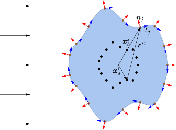
Figure 1: Schematic diagram of a flow past an object of an arbitrary shape depicting the boundary discretization and the placement of singularities outside the flow domain. The red and blue arrows at each boundary node depict the normal (pointing toward the flow domain) and tangential directions at that node, respectively.

In the MFS, it is quite natural to place the singularity points outside the flow domain Kupradze and Aleksidze (1964). Notwithstanding, the location of the singularity points is a major concern as the results obtained from the MFS are highly sensitive toward the location of singularities Alves (2009); Chen, Karageorghis, and Li (2016); Cheng and Hong (2020). There are two most common ways of distributing singularities in the MFS. One way is to place the singularities on a fictitious boundary of a very simple shape—irrespective of the shape of the object—with just one parameter to control; for example, on a circle in the two-dimensional case and on a sphere in the three-dimensional case, and the radius of the circle or sphere would be the controlling parameter. Another way is to recreate a dilated (or shrunk) fictitious boundary, which has the same shape as the boundary of the original object and to place the singularities on this fictitious boundary Cheng and Hong (2020); Li, Chen, and Karageorghis (2013)—similarly to that shown in Fig. 1 as well. The latter is also easy if the original boundary of the object can be described by a set of parametric equations having only a single controlling parameter, the dilation factor. For the problem depicted in Fig. 1, we have taken the fictitious boundary to be of the same shape as the original boundary.

Let $B$ be the number of the discretized boundary nodes and $S$ the number of singularity points. The boundary nodes and the singularities are placed at equispaced angles $\theta$ on the original and the fictitious boundary, respectively, and the distance between both boundaries can be varied by changing the value of the dilation factor $a$. It may be noted that singularities need not be placed at equispaced angles in principle; nonetheless, we have done so for the sake of simplicity. Let $\bm{x}_{i}^{s}$ and $\bm{x}_{j}^{b}$ be the position vectors of the $i^{\mathrm{th}}$ singularity site and the $j^{\mathrm{th}}$ boundary node, respectively, then the position vector from the $i^{\mathrm{th}}$ singularity site to any position $\bm{x}$ in the domain is $\bm{r}_{i}=\bm{x}-\bm{x}_{i}^{s}$ and the position vector from the $i^{\mathrm{th}}$ singularity site to the $j^{\mathrm{th}}$ boundary node is $\bm{r}_{ij}=\bm{x}_{j}^{b}-\bm{x}_{i}^{s}$. It is important to note that the subscripts ‘$i$’ and ‘$j$’ are now being used for denoting the $i^{\mathrm{th}}$ singularity site and $j^{\mathrm{th}}$ boundary node and consequently, the repetition of indices henceforth shall not imply the Einstein summation per se, unless stated otherwise (particularly, in Appendix A, wherein the Einstein summation does hold over the repeated indices). Since the point sources $\bm{f}$, $g$ and $h$—of different strengths—are to be put at each singularity site, there are four degrees of freedom corresponding to each singularity point [two scalars $g$ and $h$ from the point heat and mass sources, and two components $f_{1}$ and $f_{2}$ of the point force vector $\bm{f}=(f_{1},f_{2})^{\mathsf{T}}$]. In total, we have $4\times S$ unknowns, which are determined typically by satisfying the boundary conditions at the boundary points. Once the location of the singularity points is decided, the next step in the implementation of the MFS is superposition of the fundamental solutions associated with each singularity site, which makes sense because of the linearity of equations and gives the value of the field variables at the $j^{\mathrm{th}}$ boundary node. Superimposing the fundamental solutions (44)–(48) for each singularity site, the field variables at the $j^{\mathrm{th}}$ boundary node read

$$\bm{v}_{j} =\sum_{i=1}^{S}\bigg{[}\frac{\bm{f}_{i}\cdot\bm{A}(\bm{r}_{ij})}{8\pi\mathrm{Kn}}+\frac{1}{2\pi}\frac{c_{p}\mathrm{Kn}}{\mathrm{Pr}}\alpha_{0}^{2}\bm{f}_{i}\cdot\bm{B}(\bm{r}_{ij})+\frac{h_{i}\,\bm{r}_{ij}}{2\pi r_{ij}^{2}}\bigg{]},$$ (55)

$$p_{j} =\sum_{i=1}^{S}\frac{\bm{f}_{i}\cdot\bm{r}_{ij}}{2\pi r_{ij}^{2}},$$ (56)

$$\bm{\sigma}_{j} =\sum_{i=1}^{S}\frac{\bm{f}_{i}\cdot\bm{r}_{ij}+2\mathrm{Kn}\,(h_{i}+g_{i}\,\alpha_{0})}{2\pi}\bm{B}(\bm{r}_{ij}),$$ (57)

$$T_{j} =-\sum_{i=1}^{S}\frac{\mathrm{Pr}}{c_{p}\mathrm{Kn}}\frac{g_{i}\,\ln{r}_{ij}}{2\pi},$$ (58)

$$\bm{q}_{j} =\sum_{i=1}^{S}\bigg{[}\frac{g_{i}}{2\pi}\frac{\bm{r}_{ij}}{r_{ij}^{2}}-\frac{1}{2\pi}\frac{c_{p}\mathrm{Kn}}{\mathrm{Pr}}\alpha_{0}\bm{f}_{i}\cdot\bm{B}(\bm{r}_{ij})\bigg{]},$$ (59)

where $r_{ij}=|\bm{r}_{ij}|$; $\bm{f}_{i}=({f_{1}}_{i},{f_{2}}_{i})^{\mathsf{T}}$, $g_{i}$ and $h_{i}$ are the point force (vector), point heat source and point mass source, respectively, applied on the $i^{\mathrm{th}}$ singularity site; and

$$\bm{A}(\bm{r}_{ij})= \frac{2\bm{r}_{ij}\bm{r}_{ij}}{r_{ij}^{2}}-(2\ln{r}_{ij}-1)\bm{I},$$ (60)

$$\bm{B}(\bm{r}_{ij})= \frac{2\bm{r}_{ij}\bm{r}_{ij}}{r_{ij}^{4}}-\frac{\bm{I}}{r_{ij}^{2}}.$$ (61)

This system is solved for the unknowns ${f_{1}}_{i},{f_{2}}_{i},g_{i},h_{i}$, $i\in\{1,2,3,\dots,S\}$ by employing the boundary conditions at each boundary node. Once the unknowns ${f_{1}}_{i},{f_{2}}_{i},g_{i},h_{i}$ for $i\in\{1,2,3,\dots,S\}$ are found, the flow variables at any position $\bm{x}$ in the flow domain can be determined simply by dropping the subscript ‘$j$’ everywhere in Eqs. (55)–(59). For instance, the velocity $\bm{v}\equiv\bm{v}(\bm{x})$ at a position $\bm{x}$ in the flow domain is given by

$$\bm{v} =\sum_{i=1}^{S}\bigg{[}\frac{\bm{f}_{i}\cdot\bm{A}(\bm{r}_{i})}{8\pi\mathrm{Kn}}+\frac{h_{i}}{2\pi}\frac{\bm{r}_{i}}{r_{i}^{2}}+\frac{c_{p}\mathrm{Kn}\alpha_{0}^{2}}{2\pi\mathrm{Pr}}\bm{f}_{i}\cdot\bm{B}(\bm{r}_{i})\bigg{]}.\!$$ (62)

The other flow variables are obtained from Eqs. (56)–(59) analogously. The above procedure to evaluate flow variables works for any geometry and we have implemented this in a numerical framework. We shall elaborate on the placement of boundary nodes and source points, formation and solution of the system separately corresponding to the two problems in Sec. V and Sec. VI.

V Vapor flow confined between two coaxial cylinders

For the validation of the developed numerical framework, we revisit the problem of a rarefied vapor flow confined between two concentric cylinders. The same problem was investigated by Onishi Onishi (1977) with the linearized BGK model and the diffuse reflection boundary conditions.

V.1 Problem description

Let us consider a moderately rarefied vapor confined between the condensed phases of two concentric infinitely long circular cylinders of radii $\tilde{R}_{1}$ and $\tilde{R}_{2}$, where $\tilde{R}_{1}<\tilde{R}_{2}$. Owing to the axial symmetry along $\tilde{z}$ axis, it is sufficient to investigate the problem in 2D. A cross-sectional (two-dimensional) view of the problem is illustrated in Fig. 2.

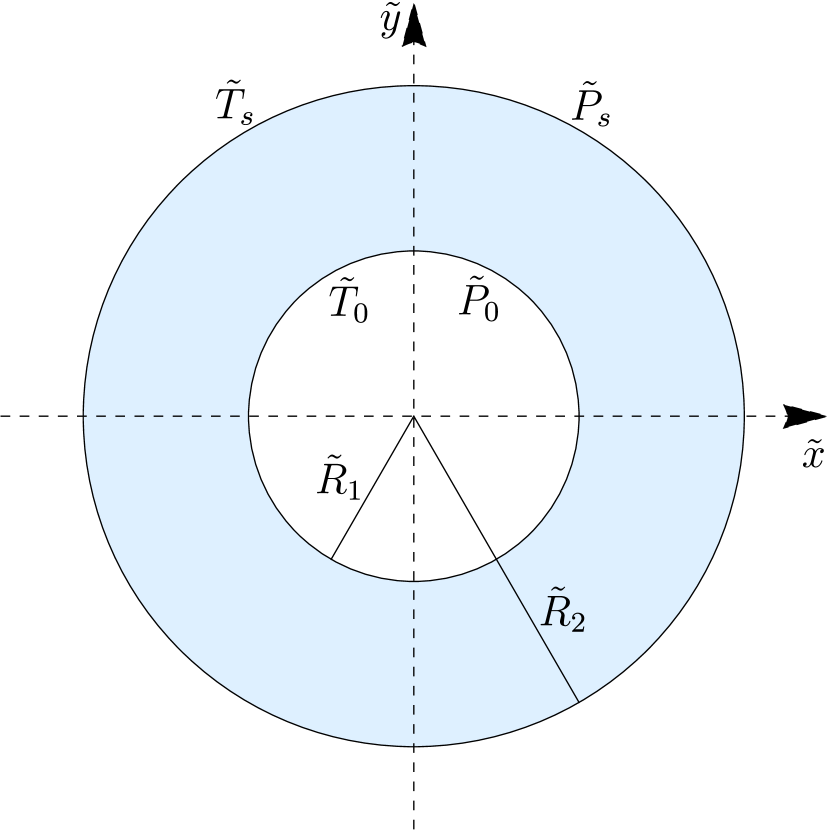
Figure 2: Cross-sectional view of the vapor flow confined between two coaxial cylinders.

For the purpose of non-dimensionalization, we take the inner radius as the characteristic length $\tilde{L}$, i.e. $\tilde{L}=\tilde{R}_{1}$. Consequently, the dimensionless radii of the inner and outer cylinders are $r_{1}=\tilde{R}_{1}/\tilde{L}=1$ and $r_{2}=\tilde{R}_{2}/\tilde{L}$, respectively. The condensed phases of the vapor at the inner and outer cylinders are assumed to be negligibly thin. Let the temperatures of the inner and outer condensed phases be maintained at uniform temperatures $\tilde{T}_{0}$ and $\tilde{T}_{s}$, respectively. Moreover, let the saturation pressures of the condensed phases corresponding to the temperatures $\tilde{T}_{0}$ and $\tilde{T}_{s}$ be $\tilde{P}_{0}$ and $\tilde{P}_{s}$, respectively; see Fig. 2. Again, for the purpose of linearization and non-dimensionalization, we take the temperature at the inner wall $\tilde{T}_{0}$ as the reference temperature and the saturation pressure at the inner wall $\tilde{P}_{0}$ as the reference pressure. Thus, the dimensionless perturbations in the temperature and saturation pressure at the inner wall vanish, and the dimensionless perturbations in the temperature and saturation pressure at the outer wall read

$$\tau_{s}=\frac{\tilde{T}_{s}-\tilde{T}_{0}}{\tilde{T}_{0}}\quad\text{and}\quad p_{s}=\frac{\tilde{P}_{s}-\tilde{P}_{0}}{\tilde{P}_{0}},$$ (63)

respectively.

V.2 Analytic solution of Onishi Onishi (1977)

Onishi Onishi (1977) investigated the problem by employing an asymptotic theory Sone (2002). According to this theory, a field variable $\tilde{h}$ of the gas can be written as

$$\tilde{h}=\tilde{h}_{H}+\tilde{h}_{K},$$ (64)

where $\tilde{h}_{H}$ is referred to as the hydrodynamic part or the Hilbert part that describes the flow behavior in the bulk of the domain and $\tilde{h}_{K}$ is referred to as the kinetic boundary layer part or the Knudsen layer part that can be seen as a correction to the Hilbert part and is significant only in a small layer near an interface. Both $\tilde{h}_{H}$ and $\tilde{h}_{K}$ for all field variables are expanded in power series of the Knudsen number, and the contribution at each power of the Knudsen number is then computed by means of the considered model (the BGK model in [Onishi, 1977]) and appropriate boundary conditions (the diffuse reflection boundary conditions in [Onishi, 1977]).

The linearized CCR model is anyway not able to predict Knudsen layers. Therefore, it makes sense to compare the results obtained from the MFS only with the Hilbert part of the solution given in Ref. [Onishi, 1977]. For the problem under consideration and for the linearized BGK model with the diffuse reflection boundary conditions, the Hilbert part of the solution is indeed straightforward to determine by solving a set of simple ordinary differential equations analytically, see Ref. [Onishi, 1977]. Denoting the radius ratio by $\beta=r_{2}/r_{1}$ and the ratio of $p_{s}$ to $\tau_{s}$ by $\gamma=p_{s}/\tau_{s}$, the analytic solution obtained from the linearized BGK model with the diffuse reflection boundary conditions for $\mathrm{Kn}\approx 0$ is given by Onishi (1977)

$$p= \medspace p_{s}\left(\frac{1}{r_{1}}+\frac{1}{r_{2}}\right)^{-1}\frac{1}{r_{1}},$$ (65)

$$v_{r}= -\frac{p_{s}}{C_{0}}\left(\frac{1}{r_{1}}+\frac{1}{r_{2}}\right)^{-1}\frac{1}{r},$$ (66)

$$T= \medspace\tau_{s}\left[\left(1-\frac{D_{0}}{C_{0}}\gamma\right)\frac{\ln{r}}{\ln{\beta}}-\left(1-\frac{D_{0}}{C_{0}}\gamma\right)\frac{\ln{r}_{1}}{\ln{\beta}}\right]$$

$$+\frac{D_{0}}{C_{0}}\gamma\tau_{s}\left(\frac{1}{r_{1}}+\frac{1}{r_{2}}\right)^{-1}\frac{1}{r_{1}},$$ (67)

$$q_{r}= 0,$$ (68)

where $C_{0}=2.132039$ and $D_{0}=0.4467494$.

V.3 Boundary conditions and implementation of the MFS

We shall revisit the problem described above by means of the MFS applied on the linearized CCR model. Recall that we have already determined the fundamental solutions of the linearized CCR model and outlined the way to implement them in Sec. III for a general two-dimensional object. The solution for the field variables at the $j^{\mathrm{th}}$ boundary node (Eqs. (44)–(48)) can directly be used once the boundary nodes and singularity points for the present problem have been decided.

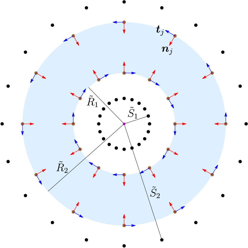
Figure 3: Schematic of the boundary nodes on the boundaries and singularity points outside the flow domain for the problem illustrated in Fig. 2. The red and blue arrows at each boundary node depict the normal (pointing toward the flow domain) and tangential directions at that node, respectively.

Since the singularity sites are to be placed outside of the computational domain, we assume the source points to be placed on two fictitious circular boundaries, one inside the circle associated with the inner cylinder and the other outside the circle associated with the outer cylinder, as shown in Fig. 3. Note that both fictitious boundaries are concentric with the circles associated with the cylinders. Let the radii of the inner and outer fictitious boundaries be $\tilde{S}_{1}$ and $\tilde{S}_{2}$, respectively. For simplicity, we consider $N_{s}$ equispaced source points on each of the two fictitious boundaries and $N_{b}$ equispaced boundary nodes on each of the actual boundaries (the boundaries of the inner and outer cylinders). As explained in Sec. IV, we have four degrees of freedom corresponding to each source point, and the total number of singularity points for the problem under consideration is $S=2N_{s}$. Thus, there will be a total of $4\times S=4\times 2N_{s}$ unknowns in the problem. Accordingly, the summations in Eqs. (44)–(48) will run from $i=1$ to $i=2N_{s}$.

Boundary conditions at the $j^{\mathrm{th}}$ boundary node are obtained from (II)–(17) by replacing the flow variables and the normal and tangent vectors with their respective values at the $j^{\mathrm{th}}$ boundary node. Furthermore, since the walls of the cylinders are fixed, $\bm{v}^{I}=\bm{0}$. Consequently, the boundary conditions at the $j^{\mathrm{th}}$ boundary node read

$$\bm{v}_{j}\cdot\bm{n}_{j}= -\eta_{11}(p_{j}-p_{\mathrm{sat}}+\bm{n}_{j}\cdot\bm{\sigma}_{j}\cdot\bm{n}_{j})$$

$$+\eta_{12}(T_{j}-T^{I}+\alpha_{0}\bm{n}_{j}\cdot\bm{\sigma}_{j}\cdot\bm{n}_{j}),$$ (69)

$$\bm{q}_{j}\cdot\bm{n}_{j}= \medspace\eta_{12}(p_{j}-p_{\mathrm{sat}}+\bm{n}_{j}\cdot\bm{\sigma}_{j}\cdot\bm{n}_{j})$$

$$-(\eta_{22}+2\tau_{0})(T_{j}-T^{I}+\alpha_{0}\bm{n}_{j}\cdot\bm{\sigma}_{j}\cdot\bm{n}_{j}),$$ (70)

$$\bm{t}_{j}\cdot\bm{\sigma}_{j}\cdot\bm{n}_{j}= -\varsigma(\bm{v}_{j}+\alpha_{0}\bm{q}_{j})\cdot\bm{t}_{j}.$$ (71)

The dimensionless perturbations in saturation pressures at the inner and outer interfaces are $p_{\mathrm{sat}}=0$ and $p_{\mathrm{sat}}=p_{s}$, respectively, and the dimensionless perturbations in temperatures at the inner and outer interfaces are $T^{I}=0$ and $T^{I}=\tau_{s}$, respectively, which need to be replaced in boundary conditions (V.3)–(71) accordingly. Note that boundary conditions (V.3)–(71) are to be satisfied at $B=2N_{b}$ boundary nodes. On substituting the values of the field variables at the $j^{\mathrm{th}}$ boundary node from (55)–(59) into boundary conditions (V.3)–(71), the resulting system of equations (associated with the $j^{\mathrm{th}}$ boundary node) can be written in a matrix form as

$$\sum_{i=1}^{S}M_{ji}\bm{u}_{i}=\bm{b}_{j},$$ (72)

for the unknown vector associated with the $i^{\mathrm{th}}$ singularity $\bm{u}_{i}=({f_{1}}_{i},{f_{2}}_{i},g_{i},h_{i})^{\mathsf{T}}$. Here, $M_{ji}$’s are coefficient matrices of dimensions $3\times 4$ and $\bm{b}_{j}$ is the $3\times 1$ vector containing the interface properties, such as $p_{s}$ and $\tau_{s}$. We collect all such $B$ systems into a new system

$$\mathcal{M}\bm{\mathcal{X}}=\bm{\mathcal{B}},$$ (73)

where $\bm{\mathcal{X}}=\big{(}{f_{1}}_{1},{f_{2}}_{1},g_{1},h_{1},{f_{1}}_{2},{f_{2}}_{2},g_{2},h_{2},\dots,{f_{1}}_{S},{f_{2}}_{S},\allowbreak g_{S},h_{S}\big{)}^{\mathsf{T}}$ is the vector containing all $4S$ unknowns, the matrix $\mathcal{M}$—containing the coefficients of the unknowns—has dimensions $3B\times 4S$ (or $6N_{b}\times 8N_{s}$) and is referred to as the collocation matrix. We have solved system (73) in the computer algebra software, Mathematica^® using the method of least squares. For the identification purpose, the first $N_{s}$ singularity points ($i=1,2,\dots,N_{s}$) in our code belong to the inner fictitious boundary and the rest $N_{s}$ singularity points ($i=N_{s}+1,N_{s}+2,\dots,2N_{s}$) to the outer fictitious boundary. Similarly, the first $N_{b}$ boundary nodes ($j=1,2,\dots,N_{b}$) belong to the actual inner boundary and the rest $N_{b}$ boundary nodes ($j=N_{b}+1,N_{b}+2,\dots,2N_{b}$) to the actual outer boundary.

V.4 Results and discussion

For numerical computations, we have taken $N_{b}=100$ boundary nodes on each of the actual boundaries and $N_{s}=100$ singularity points on each of the fictitious boundaries. The dimensionless radii of the original and fictitious boundaries are taken as $r_{1}=1$, $r_{2}=2$, $s_{1}=\tilde{S}_{1}/\tilde{R}_{1}=0.5$ and $s_{2}=\tilde{S}_{2}/\tilde{R}_{1}=4$.

Figure 4 illustrates the variation of the (scaled) temperature of the vapor in the radial direction for $\mathrm{Kn}\approx 0$ and for different values of the parameter $\gamma\,(=p_{s}/\tau_{s})$, wherein $\tau_{s}=4$ is fixed and $p_{s}$ is being varied for varying $\gamma$. The solid lines represent the results obtained from our numerical framework based on the MFS while the symbols delineate the results from Eq. (V.2), which was obtained analytically for $\mathrm{Kn}\approx 0$ through an asymptotic theory Sone (2002) performed on the linearized BGK model in Ref. [Onishi, 1977]. It is evident from the figure that the results obtained with the MFS in the present work are in an excellent agreement with the analytic results from the linearized BGK model for $\mathrm{Kn}\approx 0$.

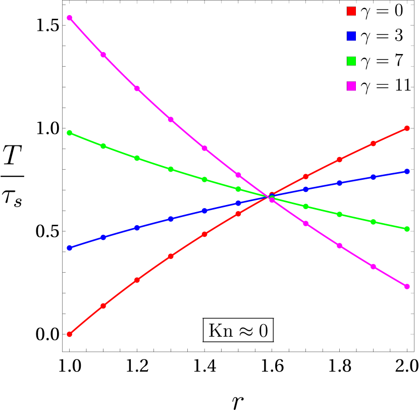
Figure 4: Variation of the (scaled) temperature in the gap between the two cylinders for different values of $\gamma$. The solid lines denote the results obtained from the MFS applied on the CCR model and the symbols indicate the analytic results from Eq. (V.2), which was obtained analytically from the linearized BGK model for $\mathrm{Kn}\approx 0$ in Ref. [Onishi, 1977]. The other parameters are $N_{b}=100$, $N_{s}=100$, $r_{1}=1$, $r_{2}=2$, $s_{1}=0.5$ and $s_{2}=4$.

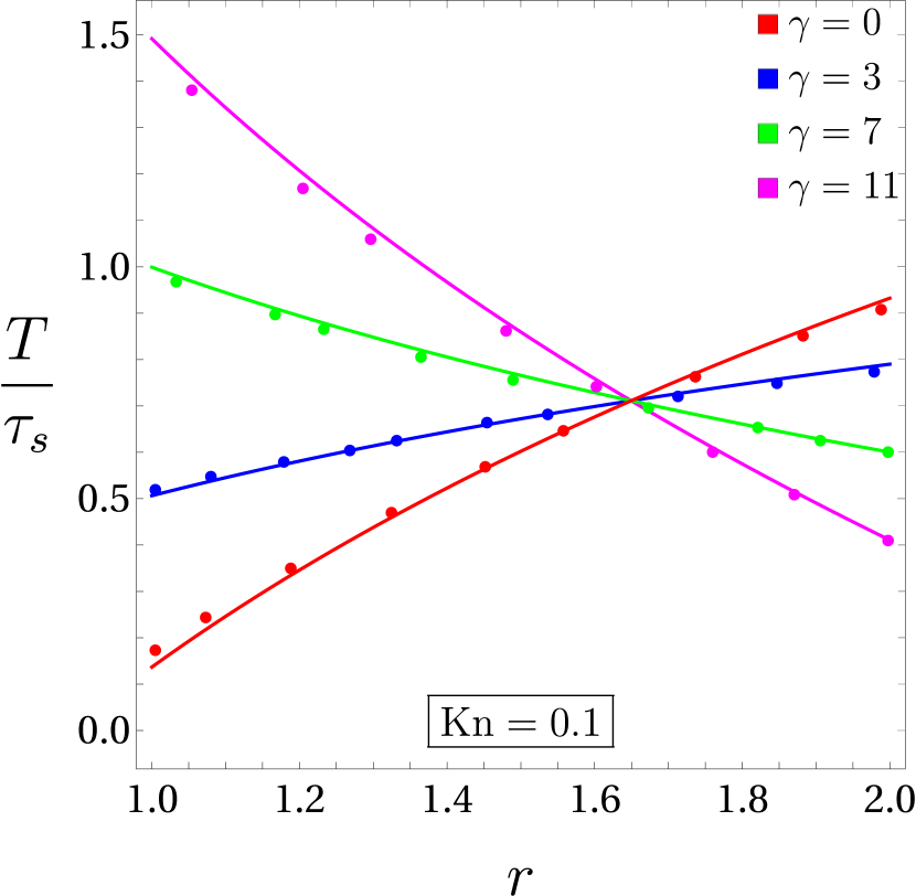
Figure 5: Same as Fig. 4 except for the symbols denote the data from Ref. [Onishi, 1977] for $\mathrm{Kn}=0.1$ obtained using the linearized BGK model.

Although not shown here for brevity, the results for the pressure and velocity from the MFS are also in excellent agreement with the analytic results from Eqs. (65) and (66) for $\mathrm{Kn}\approx 0$. It is also evident from Fig. 4 that the temperature increases on moving away from the inner cylinder toward the outer cylinder for smaller values of $\gamma$ (red and blue curves and symbols in the figure) and vice versa for larger values of $\gamma$ (green and magenta curves and symbols in the figure). This indicates the existence of a reverse temperature gradient after a critical value of $\gamma$. Indeed, at this critical value of $\gamma$, the (scaled) temperature remains constant along the radial direction. An expression for this critical value of $\gamma$ from the asymptotic theory Sone (2002) is given by Onishi (1977)

$$\gamma_{c}=\frac{C_{0}}{D_{0}}\left[1-\mathrm{Kn}\frac{C_{0}}{D_{0}}(0.124226)\left(\frac{1}{r_{1}}-\frac{1}{r_{2}}\right)+\mathcal{O}(\mathrm{Kn}^{2})\right].$$ (74)

For $\mathrm{Kn}\approx 0$, the critical value of $\gamma$ from the above expression is $\gamma_{c}=C_{0}/D_{0}\approx 4.772337$. From the MFS presented here, the critical value of $\gamma$ for $\mathrm{Kn}\approx 0$ turns out to be $\gamma_{c}\approx 4.7723$, which is also very close to that computed from the above expression. The phenomenon of reverse temperature gradient can be understood form boundary condition (V.3) as follows. There are two factors determining the normal heat flux component in boundary condition (V.3) according to which the evaporation/condensation rate depends on (i) the difference between the pressure and saturation pressure, and (ii) the temperature difference between the temperatures of the gas (or vapor) and and interface. The temperature gradient gets reversed when one dominates the other.

To examine the capabilities of the developed method, we also study the problem for higher Knudsen numbers. Figure 5 exhibits the variation of the (scaled) temperature of the vapor in the radial direction for $\mathrm{Kn}=0.1$ and for different values of the parameter $\gamma$. The solid lines again represent the results obtained from our numerical framework based on the MFS but the symbols now denote the data from the linearized BGK model taken directly from Ref. [Onishi, 1977]. It is clear from the figure that the results from the MFS are in good agreement with those from the linearized BGK model even for $\mathrm{Kn}=0.1$; nonetheless, the quantitative differences in the results from both methods are now noticeable. In addition, Fig. 5 also shows the existence of a reverse temperature gradient. For $\mathrm{Kn}=0.1$, the critical value of $\gamma$, at which the phenomenon of reverse temperature gradient occurs, computed from the MFS is $\gamma_{c}=4.66247$ whereas its reported value from the linearized BGK model in Ref. [Onishi, 1977] is $\gamma_{c}=4.63087$.

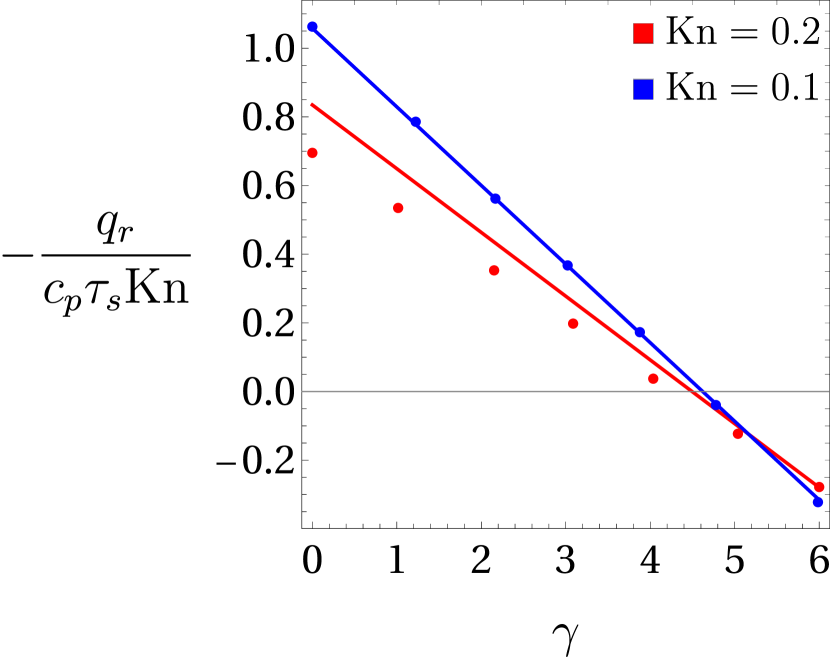
Figure 6: Variation of the (scaled) radial heat flux with $\gamma$. The solid lines denote the results obtained from the MFS applied on the CCR model and the symbols indicate the data taken directly from Ref. [Onishi, 1977], which were obtained using the linearized BGK model. The other parameters are the same as those for Fig. 4.

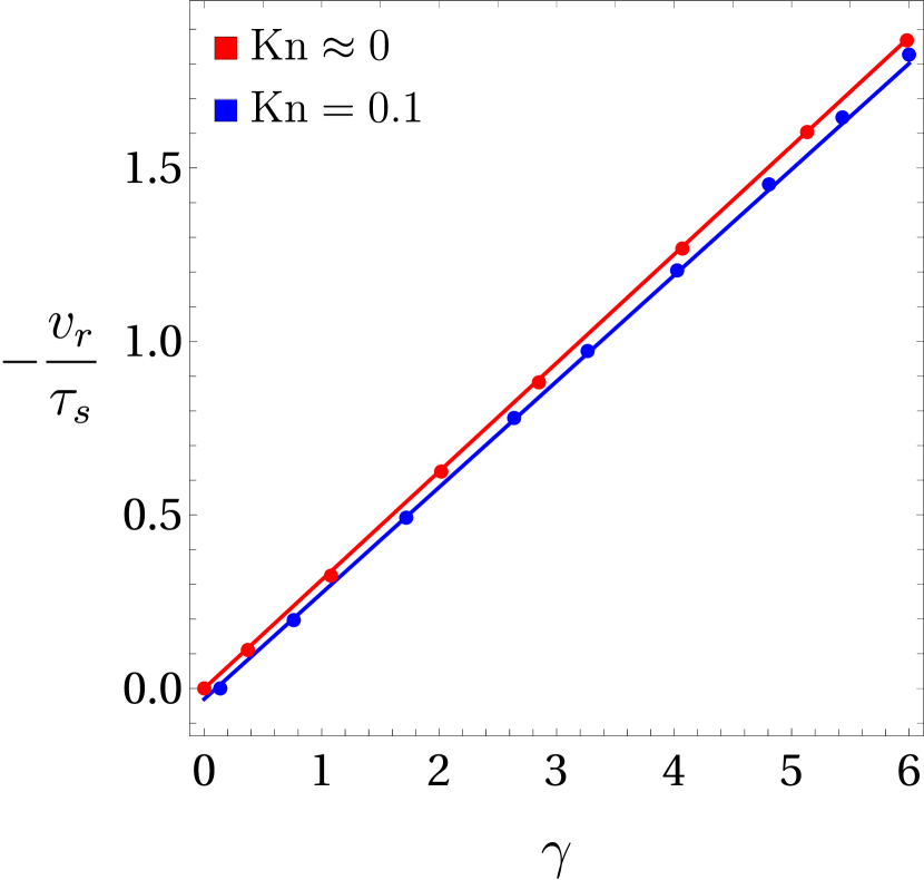
Figure 7: Variation of the (scaled) radial velocity with $\gamma$. The solid lines denote the results obtained from the MFS applied on the CCR model and the symbols indicate those from the linearized BGK model (from Eq. (66) in the case of $\mathrm{Kn}\approx 0$ and directly from Ref. [Onishi, 1977] in the case of $\mathrm{Kn}=0.1$). The other parameters are the same as those for Fig. 4.

To have further insight on the reverse temperature gradient, the (scaled) radial heat flux at the actual inner boundary (i.e. at $r=1$) is plotted against $\gamma$ in Fig. 6. The solid lines and symbols denote the results from the MFS in the present work and the data from the linearized BGK model given in Ref. [Onishi, 1977], respectively. It is apparent from the figure that our results for the radial heat flux are also in good agreement with the data from the linearized BGK model for a smaller value of the Knudsen number ($\mathrm{Kn}=0.1$ in the figure); however, for a higher value of the Knudsen number ($\mathrm{Kn}=0.2$ in the figure), there is a noticeable mismatch between the results obtained from the MFS and the data from the linearized BGK model given in Ref. [Onishi, 1977]. A plausible reason for this discrepancy could be the truncation of power series at the first order in Ref. [Onishi, 1977] because the neglected terms in the series could have significant contributions for larger values of the Knudsen number. Figure 6 also shows that for each value of the Knudsen number, there is a $\gamma$ at which the radial heat flux changes its sign. This $\gamma$ is indeed the same as the $\gamma_{c}$ described above, at which reversal of the temperature gradient takes place.

Through the plots of heat flux lines, also not shown here for brevity, it has been found that, in the case of $\tau_{s}>0$, heat flows from the outer cylinder toward the inner cylinder for $\gamma<\gamma_{c}$ and vice versa for $\gamma>\gamma_{c}$ . This makes sense in view of Figs. 4 and 5. The direction of heat flow reverses in both cases when $\tau_{s}$ is taken to be negative or, in other words, when the initial temperature of the inner cylinder is taken higher than that of the outer cylinder.

Figure 7 displays the (scaled) radial velocity plotted against $\gamma$ for $\mathrm{Kn}\approx 0$ and $\mathrm{Kn}=0.1$. The solid lines are again the results from the MFS in the present work while the symbols in the case of $\mathrm{Kn}\approx 0$ denote the results from Eq. (66) and those in the case of $\mathrm{Kn}=0.1$ denote the data taken from Ref. [Onishi, 1977]; nevertheless, in both cases symbols denote the results from the linearized BGK model. The figure also demonstrates a good agreement between the results from the method developed in the present work and those from the linearized BGK model.

VI Rarefied gas flow between two non-coaxial cylinders

In this section, we revisit the problem of flow induced by a temperature difference in a rarefied gas confined between two non-coaxial cylinders via the MFS developed above. The same problem was investigated numerically by Aoki, Sone and Yano Aoki, Sone, and Yano (1989) with the linearized BGK model and the diffuse reflection boundary conditions.

VI.1 Problem description

Let us consider a rarefied (monatomic) gas confined between two infinitely long circular cylinders of radii $\tilde{R}_{1}$ and $\tilde{R}_{2}$ (with $\tilde{R}_{1}<\tilde{R}_{2}$) that are not coaxial. Again, owing to the axial symmetry, it is sufficient to investigate the problem in 2D.

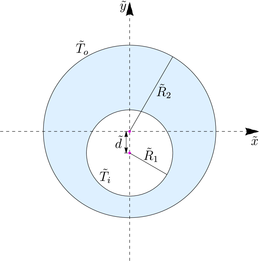
Figure 8: Cross-sectional view of the flow of a rarefied gas confined between two non-coaxial cylinders having different wall temperatures.

Let the locations of both cylinders be fixed according to the cross-sectional view portrayed in Fig. 8 so that the centers of the circles associated with the inner and outer cylinders be at the origin and at $(0,-\tilde{d})$, respectively. Furthermore, let the temperatures of the inner and outer cylinders be kept fixed at $\tilde{T}_{i}=\tilde{T}_{0}$ and $\tilde{T}_{o}=\tilde{T}_{0}(1+\Delta\tau)$, respectively, with $\Delta\tau$ being sufficiently small in comparison to $\tilde{T}_{0}$ so that the linear theory remains meaningful.

For the purpose of non-dimensionalization, we again take the radius of the inner cylinder as the characteristic length $\tilde{L}$, i.e. $\tilde{L}=\tilde{R}_{1}$. Consequently, the dimensionless radii of the inner and outer cylinders are $r_{1}=\tilde{R}_{1}/\tilde{L}=1$ and $r_{2}=\tilde{R}_{2}/\tilde{L}$, respectively, and the dimensionless distance between the centers of the cylinders is $d=\tilde{d}/\tilde{L}$. Furthermore, for the purpose of the linearization and non-dimensionalization, the equilibrium pressure of the gas $\tilde{p}_{0}$ is taken as the reference pressure and the temperature of the inner cylinder $\tilde{T}_{i}$ as the reference temperature so that the dimensionless perturbations in temperatures on the inner and outer walls are $T_{i}=(\tilde{T}_{i}-\tilde{T}_{i})/\tilde{T}_{i}=0$ and $T_{o}=(\tilde{T}_{o}-\tilde{T}_{i})/\tilde{T}_{i}=\Delta\tau$, respectively. For comparing the results from the present method with those of Ref. [Aoki, Sone, and Yano, 1989], the parameters are fixed to $r_{2}=2$, $d=0.5$ and $\Delta\tau=1$.

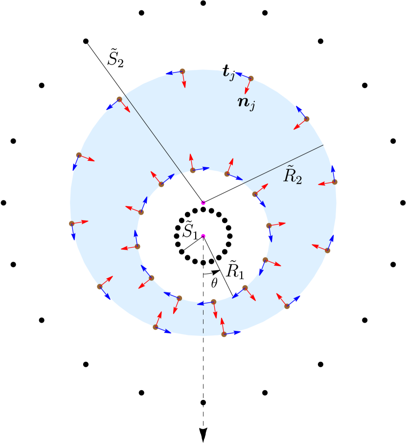
Figure 9: Schematic of the boundary nodes on the boundaries and singularity points outside the flow domain for the problem illustrated in Fig. 8. The red and blue arrows at each boundary node depict the normal (pointing toward the flow domain) and tangential directions at that node, respectively.

VI.2 Boundary Conditions and implementation of the MFS

In order to place the singularity sites outside the computational domain, we again assume the source points to be placed on two fictitious circular boundaries, one inside the circle associated with the inner cylinder and the other outside the circle associated with the outer cylinder, as shown in Fig. 9. The inner (outer) fictitious boundary is concentric with the circle associated with the inner (outer) cylinder. Let the radii of the inner and outer fictitious boundaries be $\tilde{S}_{1}$ and $\tilde{S}_{2}$, respectively. Consequently, the dimensionless radii of the inner and outer fictitious boundaries are $s_{1}=\tilde{S}_{1}/\tilde{L}$ and $s_{2}=\tilde{S}_{2}/\tilde{L}$. Similarly to the above, we consider $N_{s}$ equispaced source points on each of the two fictitious boundaries and $N_{b}$ equispaced boundary nodes on each of the actual boundaries (the boundaries of the inner and outer cylinders).

Since the walls of the cylinders are fixed for this problem as well, $\bm{v}^{I}=\bm{0}$. Hence, the boundary conditions (V.3)–(71) at the $j^{\mathrm{th}}$ boundary node hold true for the present problem as well. However, since the present problem does not involve evaporation and condensation, the evaporation/condensation coefficient $\vartheta$ is zero for this problem. Consequently, boundary conditions (V.3)–(71) for the problem under consideration further reduce to

$$\bm{v}_{j}\cdot\bm{n}_{j} =0,$$ (75)

$$\bm{q}_{j}\cdot\bm{n}_{j} =-2\tau_{0}(T_{j}-T^{I}+\alpha_{0}\,\bm{n}_{j}\cdot\bm{\sigma}_{j}\cdot\bm{n}_{j}),$$ (76)

$$\bm{t}_{j}\cdot\bm{\sigma}_{j}\cdot\bm{n}_{j} =-\varsigma(\bm{v}_{j}+\alpha_{0}^{\prime}\bm{q}_{j})\cdot\bm{t}_{j}.$$ (77)

Note that the coefficient $\alpha_{0}$ in boundary condition (77) has been changed to $\alpha_{0}^{\prime}=1/5$ (see, e.g., Refs. [Struchtrup, 2005; Struchtrup and Torrilhon, 2008; Taheri, Torrilhon, and Struchtrup, 2009]) in order to have a fair comparison with the findings of Ref. [Aoki, Sone, and Yano, 1989]. The interface temperature $T^{I}$ in boundary condition (76) is $0$ for the inner cylinder and $\Delta\tau$ for the outer cylinder.

The construction of the collocation matrix and the formation of system (73) for the present problem is exactly similar to that demonstrated in Sec. V.3. We have again solved system (73) for the present problem analogously in the computer algebra software, Mathematica^® using the method of least squares to determine the unknowns ${f_{1}}_{1},{f_{2}}_{1},g_{1},h_{1},{f_{1}}_{2},{f_{2}}_{2},g_{2},h_{2},\dots,{f_{1}}_{S},{f_{2}}_{S},\allowbreak g_{S},h_{S}$.

VI.3 Results and discussion

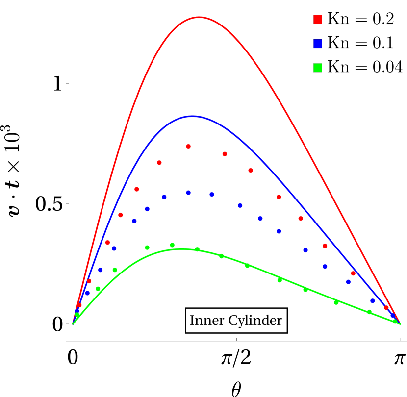
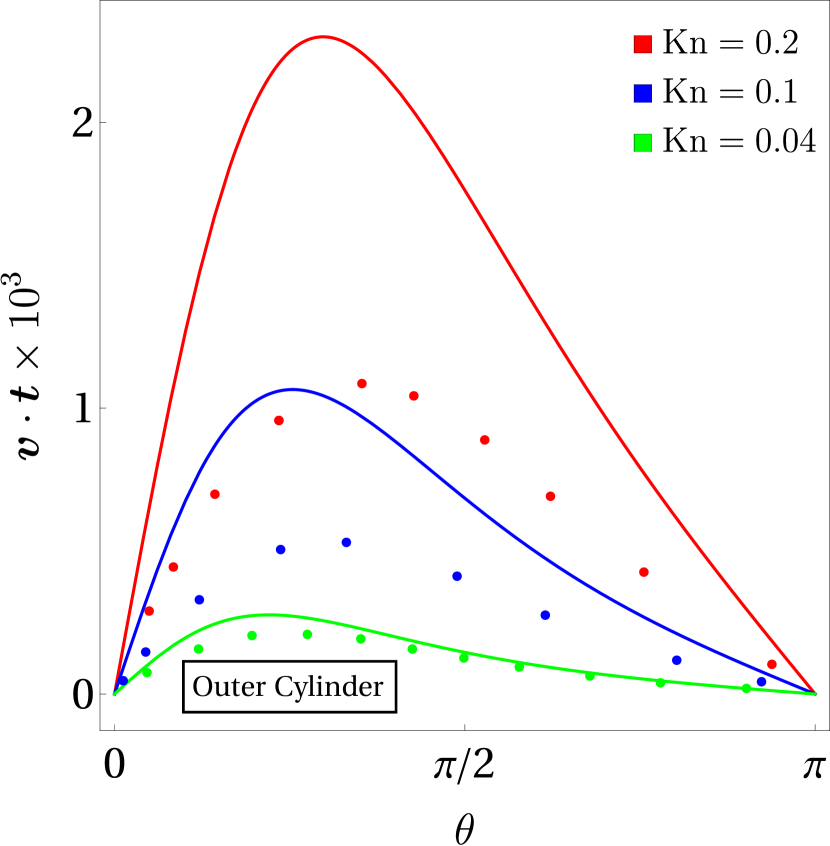
Figure 10: Tangential velocity on the right halves of the inner and outer circles associated with the respective cylinders plotted against the angle $\theta$ for different values of the Knudsen number and for $\Delta\tau=1$. The solid lines denote the results obtained from the MFS applied on the CCR model and the symbols indicate the data from the linearized BGK model Aoki, Sone, and Yano (1989). The other parameters are the same as those for Fig. 4.

We have computed the results numerically by taking the parameters as $\Delta\tau=1$, $N_{b}=N_{s}=100$, $r_{1}=1$, $r_{2}=2$, $s_{1}=0.5$ and $s_{2}=4$. In all the figures (except for Fig. 12) below, the solid lines represent the results obtained with the MFS applied on the CCR model in the present work and the symbols denote the data taken from Ref. [Aoki, Sone, and Yano, 1989], which were obtained using the linearized BGK model.

Figure 10 illustrates the variation of the tangential component of the (dimensionless) velocity on the right halves of the inner (top row) and outer (bottom row) circles associated with the respective cylinders with respect to the angle $\theta$, which is the angle measured from the negative $y$-axis anticlockwise around the center of the inner circle as shown in Fig. 9. The angle has been taken in this way in order to maintain the geometrical similarity with Ref. [Aoki, Sone, and Yano, 1989]. The unit tangential directions on the inner and outer circles are marked in Fig 9 with blue arrows. Figure 10 shows that the tangential components of the velocity for both inner and outer circles remain zero at $\theta=0$ and $\theta=\pi$ and that they attain the maximum values somewhere in $(0,\pi/2)$. Furthermore, the value of $\theta$ at which the maximum is attained also shifts more toward $\theta=\pi/2$ on increasing the value of the Knudsen number. Figure 10 evinces that the results from the MFS applied on the CCR model (solid lines) are in reasonably good agreement with those from the linearized BGK model for small Knudsen numbers (green lines and symbols) and that the differences between the results from both methods become more and more prominent with increasing Knudsen numbers (red and blue lines and symbols), where the present method starts overpredicting the results, though the trends from both methods remain qualitatively similar to each other even for high Knudsen numbers. The reason for these quantitative mismatches for large Knudsen numbers is attributed to the limitation of the CCR model in capturing the Knudsen layers, which are more conspicuous near the boundaries for large Knudsen numbers. The thickness of the Knudsen layers increases with increasing the Knudsen number Struchtrup (2008), which renders larger deviations in the tangential component of the velocity near the inner and outer walls of the cylinders with increasing the Knudsen number.

Figure 10, in other words, also reveals that at $\theta=0$ and $\theta=\pi$ the flow can happen only in the normal directions. This prompts us to draw streamlines of the flow in Fig. 11. For explanatory purpose, we also display the temperature contours in Fig. 11.

Figure 11: Velocity streamlines and temperature contours obtained from the MFS applied on the CCR model for the problem described in Sec. VI at $\mathrm{Kn}=0.1$ and $\Delta\tau=1$. The other parameters are the same as those for Fig. 4.

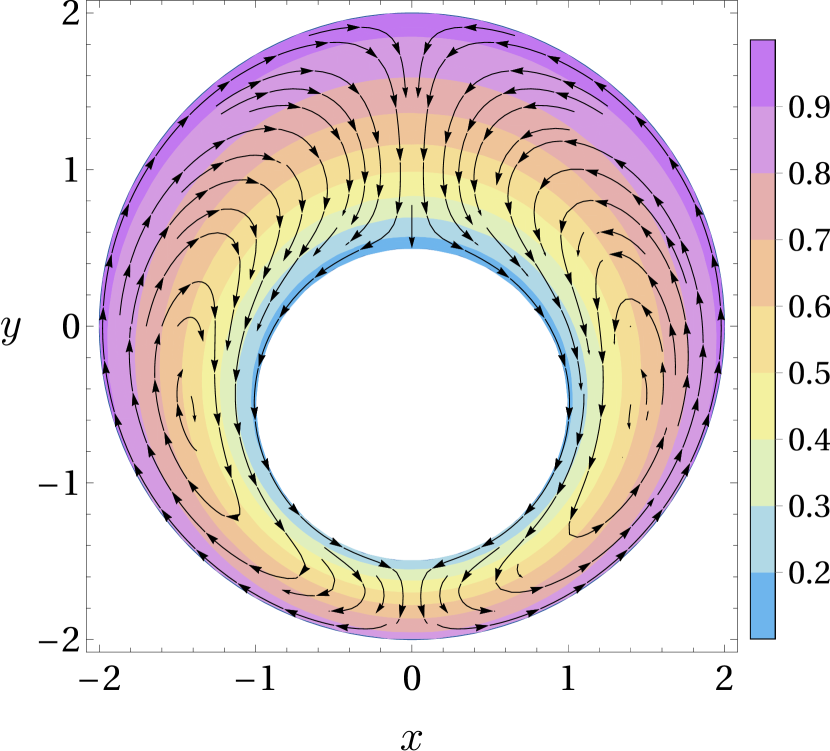
Figure 12: Velocity streamlines and temperature contours obtained from the MFS applied on the NSF equations with the second-order slip and jump boundary conditions for the problem described in Sec. VI at $\mathrm{Kn}=0.1$ and $\Delta\tau=1$. The other parameters are the same as those for Fig. 4.

The streamlines in Fig. 11 show that at the narrowest gap (at $\theta=0$), the gas starts moving from the outer (hotter) cylinder toward the inner (colder) cylinder due to the largest temperature gradient at $\theta=0$ and flows along the surface of the inner cylinder on both halves until it reaches $\theta=\pi$, at which it can flow only in the normal direction. Therefore, at the widest gap (near $\theta=\pi$), the gas flows from the inner cylinder toward the outer cylinder and returns back from there toward the narrowest gap along the surface of the outer cylinder (but in the opposite directions due to symmetry along the $y$-axis). This renders two counter-directional circulating flows, one in the left half of the domain and the other in the right half of the domain. The directions of the circulating flows reverse on taking $\Delta\tau<0$, i.e. when the inner cylinder is at a higher temperature than the outer one. With the considered values of the Knudsen number, the directions of the circulating flows apparently do not depend on the Knudsen number. The direction of the steamlines obtained from the MFS applied on the CCR model in Fig. 11 is consistent with that obtained using the linearized BGK model in Ref. [Aoki, Sone, and Yano, 1989].

In order to gain more insight into the process, we have also implemented the MFS to the (linearized) NSF equations [by setting $\alpha_{0}=0$ in Eqs. (6) and (7)] with the second-order slip and jump boundary conditions Struchtrup (2005); Struchtrup and Torrilhon (2008); Taheri, Torrilhon, and Struchtrup (2009) [obtained by setting $\alpha_{0}=1/4$ in Eq. (76) and $\alpha_{0}^{\prime}=1/5$ in Eq. (77)], and plotted the streamlines obtained with them in Fig. 12. From Figs. 11 and 12, it is evident that, in contrast to the CCR model, the NSF equations even with the second-order slip and jump boundary conditions predict streamlines in completely opposite and incorrect directions. This affirms the inadequacy of the NSF equations in describing thermal-stress slip flows (Sone, 2007) accurately, which—on the other hand—can be described reasonably well with the CCR model due to the coupling between the stress and heat flux.

The superposition of all the point force vectors at the inner source points yields the total force $\bm{F}$ acting on the inner cylinder, i.e.

$$\bm{F}=\sum_{i=1}^{N_{s}}{\bm{f}}_{i},$$ (78)

where $i=1,2,\dots,N_{s}$ refer to the points on the inner fictitious boundary. The projection of the total force in the direction opposite to the streamwise direction is referred to as the drag force (on the inner cylinder), which is given by

$$F_{d}=\bm{F}\cdot(-\hat{\bm{y}})=-\sum_{i=1}^{N_{s}}{\bm{f}}_{i}\cdot\hat{\bm{y}},$$ (79)

where $\hat{\bm{y}}$ represents the unit vector in the streamwise direction. Variation of the drag force with the Knudsen number is illustrated in Fig. 13, which shows good agreement between the results from the MFS applied on the CCR model (solid lines) and those from the linearized BGK model (symbols) even for high Knudsen numbers (especially, for $\mathrm{Kn}\lesssim 2$).

Figure 13: Drag force on the inner cylinder plotted against the Knudsen number for $\Delta\tau=1$. The solid and dashed lines denote the results obtained from the MFS applied on the CCR and NSF models, respectively, while the symbols indicate the data for the drag force obtained from the linearized BGK model Aoki, Sone, and Yano (1989). The other parameters are the same as those for Fig. 4.

This was actually not the case for tangential velocity displayed in Fig. 10, where the differences between the results from the two models were noticeable for high Knudsen numbers. This shows that the CCR model is capable of predicting the global quantities, e.g., the drag force, quite accurately but is incapacitated of predicting the local quantities, e.g., the velocity and temperature, for high Knudsen numbers due to its limitation of not being able to predict Knudsen layers. On the contrary, the drag force obtained with the NSF equations (depicted by the dashed line in Fig. 13) deviates significantly from the drag force obtained with the linearized BGK model for $\mathrm{Kn}\gtrsim 0.2$.

VII Location of singularities

As mentioned in Sec. I, the collocation matrix associated with the linear system resulting from the MFS could be ill-conditioned and there is a trade-off between the accuracy and good conditioning. Therefore, it is important to determine an appropriate location for the fictitious boundary in order to obtain the solutions with a desired accuracy.

An ill-conditioned matrix has a high condition number. Thus the MFS can yield accurate results even with the collocation matrix having a high condition number. This seems to be implausible intuitively; notwithstanding, it should be noted that the traditional condition number is not adequate for measuring the accuracy and stability of the resulting system since the condition number does not take boundary data into account. For instance, while forming matrix system (73), the boundary data, such as $p_{s}$, $\tau_{s}$ or $\Delta\tau$, for the problems investigated in this paper appear in the vector $\mathcal{B}$ but not in the collocation matrix $\mathcal{M}$. Hence, the (usual) condition number of the matrix $\mathcal{M}$ is not an adequate parameter to gauge the sensitivity of the MFS toward the location of the source points.

A more accurate estimation of the sensitivity of the MFS toward the location of the source points can be made by the effective condition number, which also takes the boundary data into account (through the right-hand side vector). The concept of the effective condition number has been used by many authors to determine an optimal location of the singularity points by conjecturing a reciprocal relationship between the inaccuracy of the MFS and the effective condition number Drombosky, Meyer, and Ling (2009); Wong and Ling (2011); Chen et al. (2023). For both the problems discussed in the above sections, we have used the same strategy to place the source points. Further details on this strategy are as follows.

Using the singular value decomposition, $\mathcal{M}$ (having dimensions $n\times m$) can be decomposed as $\mathcal{M}=UDV^{\mathsf{T}}$, where $U$ and $V$ are $n\times n$ and $m\times m$ orthogonal matrices and $D$ is a $n\times m$ diagonal matrix containing the positive singular values in descending order: $\sigma_{1}\geq\sigma_{2}\geq\sigma_{3}\geq\dots\geq\sigma_{r}>0$, where $r\leq m$. The definitions of the (traditional) condition number $\kappa$ and the effective condition number $\kappa_{\mathrm{eff}}$ in $\ell^{2}$-norm are given by

$$\kappa=\frac{\sigma_{1}}{\sigma_{r}}\quad\text{and}\quad\kappa_{\mathrm{eff}}=\frac{\|\bm{\mathcal{B}}\|}{\sigma_{r}\|\bm{\mathcal{X}}\|}.$$

Using the definition of the effective condition number, we first verify the inverse relationship between the maximum error and the effective condition number.

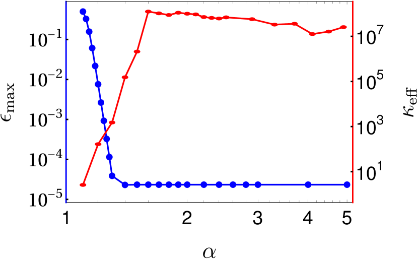
Figure 14: The maximum absolute error $\epsilon_{\max}$ in the temperature and effective condition number $\kappa_{\mathrm{eff}}$ for the problem of flow between coaxial cylinders plotted over the dilation parameter $\alpha$ for $\mathrm{Kn}\approx 0$ and $N_{b}=N_{s}=100$.

Let $\alpha>1$ be the dilation parameter that determines the separation between the actual boundary (containing boundary nodes) and the fictitious boundary (containing singularities) such that $s_{1}=r_{1}/\alpha$ and $s_{2}=\alpha\,r_{2}$. A larger value of $\alpha$ corresponds to a larger gap between the boundary nodes and source points.

For the problem described in Sec. V, the maximum absolute error $\epsilon_{\max}$ in the temperature computed with the MFS and with the analytic solution for $\mathrm{Kn}\approx 0$ along with the effective condition number is plotted against the dilation parameter $\alpha$ in Fig. 14. The figure shows that the inaccuracy of the MFS is roughly inversely proportional to the effective condition number. It is also evident from the figure that the maximum value of the effective condition number is attained for $\alpha$ around $1.6$, where the effective condition number is of order $10^{8}$ and the absolute error is minimum. It is worthwhile noting that the order of the effective condition number remains $10^{8}$ for higher values of $\alpha$ beyond $\alpha\approx 1.6$; similarly, the order of the maximum absolute error remains $10^{-5}$ for higher values of $\alpha$ beyond $\alpha\approx 1.6$.

In order to have further insight, the effective condition number for the problems considered in Sec. V and Sec. VI is plotted against the dilation parameter in Fig. 15 for different values of the Knudsen number. The number of boundary nodes at either of the actual boundaries $N_{b}$ and the number of singularity points at either of the fictitious boundaries $N_{s}$ are taken as 100 (i.e. $N_{b}=N_{s}=100$) in Fig. 15.

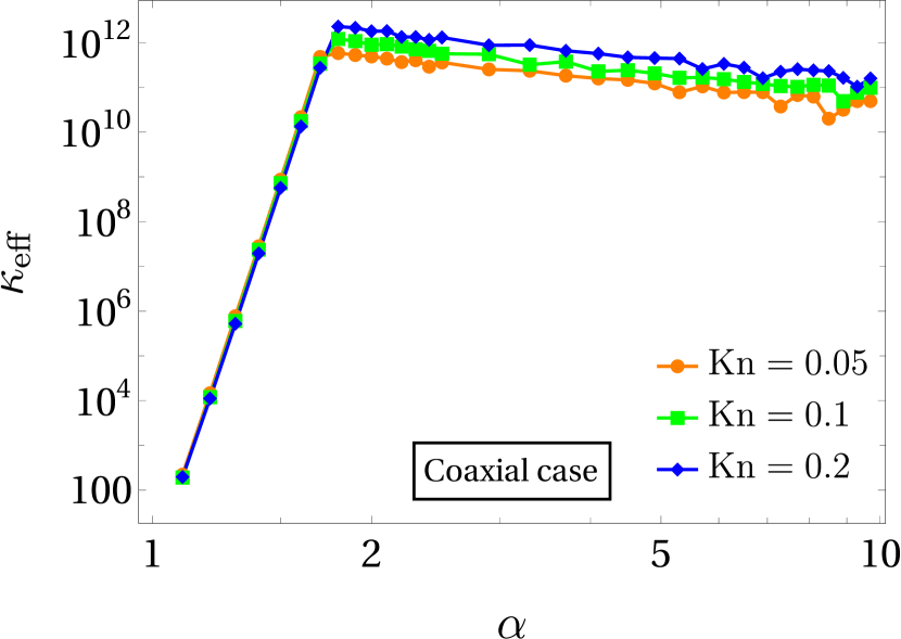
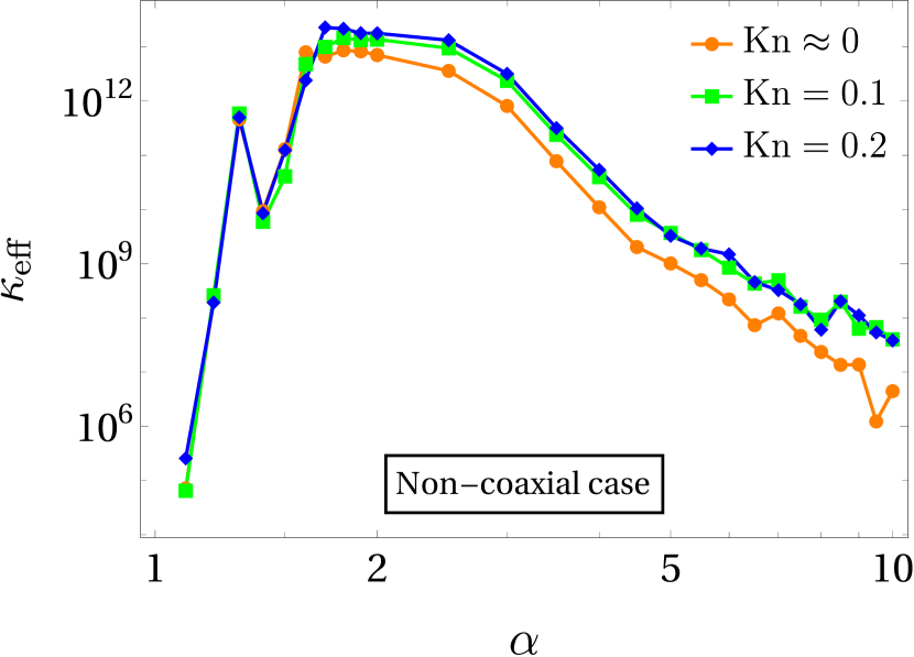
Figure 15: Variation of the effective condition number $\kappa_{\mathrm{eff}}$ with respect to the dilation parameter $\alpha$ for the problems described in Sec. V (coaxial case) and Sec. VI (non-coaxial case). The number of boundary nodes at either of the actual boundaries and the number of singularity points at either of the fictitious boundaries are 100 (i.e. $N_{b}=N_{s}=100$).

It can be noticed from the figure that the highest value of the effective condition number for a given Knudsen number is attained at a value of $\alpha$ somewhere in between $1.8$ and $2$. Although, not shown here for succinctness, it turns out that the value of $\alpha$ at which the highest effective condition number is attained increases (decreases) with decrease (increase) in the number of boundary nodes and singularities. Therefore, to save computational time, one can use smaller number of boundary nodes and source points along with a bigger value of $\alpha$. From Fig. 15, although the effective condition number decreases on increasing $\alpha$ after a certain value of $\alpha$, we have not encountered any significant change in the results on keeping the singularities farther (or on taking bigger values of $\alpha$). Therefore, it is apparently sufficient to just ensure $\alpha\geq 2$ to attain an optimal accuracy in the case of $N_{b}=N_{s}=100$. Therefore, the fictitious boundaries for both problems have safely been positioned at locations for which $\alpha=2$.

VIII Conclusion and outlook

The fundamental solutions of the CCR model in 2D have been determined by exploiting the fundamental solutions of some well-known partial differential equations, e.g., the Laplace and biharmonic equations. It turns out that the fundamental solutions of the linearized NSF and G13 equations in 2D can be recovered from the fundamental solutions of the CCR model in 2D derived in this paper by taking the coupling coefficient $\alpha_{0}$ as $0$ and $2/5$, respectively, in them. The derived fundamental solutions for the two-dimensional CCR model have then been implemented in a numerical framework.

To gauge the capability of the developed numerical framework, two problems: (i) evaporating/condensing vapor flow between two coaxial cylinders, and (ii) temperature-driven rarefied gas flow between two non-coaxial cylinders having different temperatures, have been revisited. These problems have already been investigated with the linearized BGK model in Refs. [Onishi, 1977 and Aoki, Sone, and Yano, 1989]. Comparing the results obtained from the MFS for the first problem with those from Refs. [Onishi, 1977], the accuracy of the MFS with the CCR model in investigating rarefied gas flows with phase change is vivid, particularly for small Knudsen numbers. Similarly, for the second problem, the results for the local flow fields, such as the temperature and velocity, obtained using the MFS with the CCR model compares quite well with those obtained using the linearized BGK model in the case of small Knudsen number; but the results for the local flow fields from the two models differ noticeably for larger Knudsen numbers, although their trends from both methods are qualitatively similar. On the other hand, the MFS with the CCR model is able to capture the global flow fields, such as the drag force, quite accurately even for large Knudsen numbers. In addition, since the MFS does not involve numerical computation of integrals and its implementation does not require the discretization of the domain, it is computationally efficient in comparison to the other numerical methods used for investigating rarefied gas flows. This makes the MFS with the CCR model a favorable choice for investigating rarefied gas flows. It should, however, be noted that the position of singularity points plays a major role to achieve the best results. By performing, effective condition number based studies for both problems, it has been established that the singularity points should be kept sufficiently far from the boundary nodes.

The utility of the derived fundamental solutions (and their numerical implementation) can be perceived particularly for problems wherein the quasi two-dimensional version of a problem is sufficient to study the complete problem in 3D (due to symmetry in the transverse direction) as the fundamental solutions of a model in 2D cannot be deduced directly from its counterpart in 3D and vice-versa. Since the derived fundamental solutions in this paper are not restricted to a particular geometry, the findings of this paper also open up the possibility of employing the MFS to quasi two-dimensional problems in complex geometries, for instance, to a flow confined between two right cylinders having non-circular bases. Furthermore, the derived solutions can also be extended from monatomic to polyatomic gases (of Maxwell molecules) by taking $c_{p}=(5+\mathsf{n})/2$ and $\alpha_{0}=2/(5+\mathsf{n})$, and by choosing an appropriate value of the parameter $\mathsf{n}$ that denotes the degree of freedom in a polyatomic gas.

Although the MFS is equally efficient for external flow problems as well (as demonstrated in Refs. [Lockerby and Collyer, 2016 and Rana et al., 2021]), we have not considered external flow problems in 2D as they are somewhat more involved in comparison to their 3D counterparts. This is due to Stokes’ paradox in which the solution diverges because of the presence of logarithmic term(s) in the two-dimensional fundamental solutions of Stokes’ equation. A similar logarithmic term appears in the two-dimensional fundamental solutions of the CCR model as well that makes the study of two-dimensional external flows with the MFS applied on the CCR model involved. At present, we do not have a clear understanding of dealing with Stokes’ paradox using the MFS for external flow problems, specifically for flows past an arbitrary geometry. Notwithstanding, external flows with the MFS applied on the CCR model in 2D will be considered elsewhere in the future.

IX Acknowledgement

Himanshi gratefully acknowledges the financial support from the Council of Scientific and Industrial Research (CSIR) [File No.: 09/1022(0111)/2020-EMR-I]. A.S.R. acknowledges the financial support from the Science and Engineering Research Board, India through the grants SRG/2021/000790 and MTR/2021/000417. Himanshi and V.K.G. also acknowledge the facilities of the Bhaskaracharya Mathematics Laboratory and Brahmagupta Mathematics Library supported by DST-FIST Project SR/FST/MS I/2018/26 that have been used to carry out this work.

Appendix A Inverse Fourier transforms

We use the fundamental solutions of some well-known equations, such as the Laplace and biharmonic equations, from the literature (Smyrlis, 2009; Poullikkas, Karageorghis, and Georgiou, 1998; Chen et al., 2023) to find the inverse Fourier transforms of the terms on the right-hand sides of Eqs. (33), (34) and (36)–(III). Note that the Einstein summation holds over the repeated indices in this appendix and the indices can take values $1$ and $2$ only. The fundamental solution of the Laplace equation (with a point source of unit strength)

$$\nabla^{2}\phi\equiv\frac{\partial^{2}\phi}{\partial x_{i}^{2}}=\delta(\bm{r})$$ (80)

in 2D is given by

$$\phi=\frac{\ln{r}}{2\pi}$$ (81)

where $r=|x_{i}|$.

Applying the Fourier transformation [defined by Eq. (23)] to the Laplace equation (80), we obtain

$$(-\mathbbm{i})^{2}k^{2}\hat{\phi}=1\quad\implies\quad\hat{\phi}=-\frac{1}{k^{2}}.$$ (82)

Hence, the inverse Fourier transform of $1/k^{2}$ is

$$\mathcal{F}^{-1}\left(\frac{1}{k^{2}}\right)=\mathcal{F}^{-1}(\hat{\phi})=-\frac{\ln{r}}{2\pi}.$$ (83)

Also, by definition (24), the inverse Fourier transform of $1/k^{2}$ is given by

$$\mathcal{F}^{-1}\left(\frac{1}{k^{2}}\right)=\frac{1}{(2\pi)^{2}}\int_{\mathbb{R}^{2}}\frac{1}{k^{2}}\mathrm{e}^{-\mathbbm{i}\,\bm{k}\cdot\bm{r}}\,\mathrm{d}\bm{k}.$$ (84)

Therefore, from Eqs. (83) and (84), we have

$$\frac{1}{(2\pi)^{2}}\int_{\mathbb{R}^{2}}\frac{1}{k^{2}}\mathrm{e}^{-\mathbbm{i}\,\bm{k}\cdot\bm{r}}\,\mathrm{d}\bm{k}=-\frac{\ln{r}}{2\pi}.$$ (85)

Now, taking the partial derivative with respect to $x_{i}$ on both sides in (85), we obtain

$$-\frac{\mathbbm{i}}{(2\pi)^{2}}\int_{\mathbb{R}^{2}}\frac{k_{i}}{k^{2}}\mathrm{e}^{-\mathbbm{i}\,\bm{k}\cdot\bm{r}}\,\mathrm{d}\bm{k}=-\frac{1}{2\pi}\frac{x_{i}}{r^{2}}$$ (86)

which, in turn, gives

$$\mathcal{F}^{-1}\left(\frac{k_{i}}{k^{2}}\right) =-\frac{\mathbbm{i}\,x_{i}}{2\pi r^{2}}.$$ (87)

Moreover, taking the partial derivative with respect to $x_{j}$ on both sides in (86), we obtain

$$\frac{-1}{(2\pi)^{2}}\int_{\mathbb{R}^{2}}\frac{k_{i}k_{j}}{k^{2}}\mathrm{e}^{-\mathbbm{i}\,\bm{k}\cdot\bm{r}}\,\mathrm{d}\bm{k}=-\frac{1}{2\pi}\bigg{(}\frac{\delta_{ij}}{r^{2}}-\frac{2x_{i}x_{j}}{r^{4}}\bigg{)},$$ (88)

which, in turn, gives

$$\mathcal{F}^{-1}\left(\frac{k_{i}k_{j}}{k^{2}}\right)=-\frac{1}{\pi}\frac{x_{i}x_{j}}{r^{4}}+\frac{1}{2\pi}\frac{\delta_{ij}}{r^{2}}.$$ (89)

The fundamental solution of the biharmonic equation (with a point source of unit strength)

$$\frac{\partial^{4}\phi}{\partial^{2}x_{i}\,\partial^{2}x_{j}}=\delta(\bm{r})$$ (90)

in 2D is given by

$$\phi=\frac{r^{2}\,\ln{r}}{8\pi}.$$ (91)

Following similar steps as for the Laplace equation above, we obtain

$$\mathcal{F}^{-1}\left(\frac{1}{k^{4}}\right) =\frac{r^{2}\,\ln{r}}{8\pi},$$ (92)

$$\mathcal{F}^{-1}\left(\frac{k_{i}}{k^{4}}\right) =\mathbbm{i}\frac{x_{i}(2\ln{r}+1)}{8\pi},$$ (93)

$$\mathcal{F}^{-1}\left(\frac{k_{i}k_{j}}{k^{4}}\right) =-\frac{(2\ln{r}+1)}{8\pi}\delta_{ij}-\frac{x_{i}x_{j}}{4\pi r^{2}}.$$ (94)

References

- Ohwada, Sone, and Aoki (1989) T. Ohwada, Y. Sone, and K. Aoki, “Numerical analysis of the Poiseuille and thermal transpiration flows between two parallel plates on the basis of the Boltzmann equation for hard-sphere molecules,” Phys. Fluids A 1, 2042–2049 (1989).
- Taheri, Torrilhon, and Struchtrup (2009) P. Taheri, M. Torrilhon, and H. Struchtrup, “Couette and Poiseuille microflows: Analytical solutions for regularized 13-moment equations,” Phys. Fluids 21, 017102 (2009).
- Rana et al. (2016) A. Rana, R. Ravichandran, J. H. Park, and R. S. Myong, “Microscopic molecular dynamics characterization of the second-order non-Navier-Fourier constitutive laws in the Poiseuille gas flow,” Phys. Fluids 28, 082003 (2016).
- Struchtrup and Torrilhon (2008) H. Struchtrup and M. Torrilhon, “Higher-order effects in rarefied channel flows,” Phys. Rev. E 78, 046301 (2008).
- Mohammadzadeh, Rana, and Struchtrup (2015) A. Mohammadzadeh, A. S. Rana, and H. Struchtrup, “Thermal stress vs. thermal transpiration: A competition in thermally driven cavity flows,” Phys. Fluids 27, 112001 (2015).
- Rana, Torrilhon, and Struchtrup (2013) A. Rana, M. Torrilhon, and H. Struchtrup, “A robust numerical method for the R13 equations of rarefied gas dynamics: Application to lid driven cavity,” J. Comput. Phys. 236, 169–186 (2013).
- Rana, Gupta, and Struchtrup (2018) A. S. Rana, V. K. Gupta, and H. Struchtrup, “Coupled constitutive relations: a second law based higher-order closure for hydrodynamics,” Proc. Roy. Soc. A 474, 20180323 (2018).
- Grad (1949) H. Grad, “On the kinetic theory of rarefied gases,” Comm. Pure Appl. Math. 2, 331–407 (1949).
- Rana et al. (2021) A. S. Rana, S. Saini, S. Chakraborty, D. A. Lockerby, and J. E. Sprittles, “Efficient simulation of non-classical liquid–vapour phase-transition flows: a method of fundamental solutions,” J. Fluid Mech. 919, A35 (2021).
- Modi and Rana (2022) A. Modi and A. S. Rana, “A finite difference scheme for non-Cartesian mesh: Applications to rarefied gas flows,” Phys. Fluids 34, 072002 (2022).
- Struchtrup and Torrilhon (2003) H. Struchtrup and M. Torrilhon, “Regularization of Grad’s 13 moment equations: Derivation and linear analysis,” Phys. Fluids 15, 2668–2680 (2003).
- Struchtrup (2005) H. Struchtrup, Macroscopic Transport Equations for Rarefied Gas Flows (Springer, Berlin, 2005).
- Gu and Emerson (2009) X.-J. Gu and D. R. Emerson, “A high-order moment approach for capturing non-equilibrium phenomena in the transition regime,” J. Fluid Mech. 636, 177–216 (2009).
- Lamb (1932) H. Lamb, Hydrodynamics (Cambridge University Press, Cambridge, 1932).
- Kupradze and Aleksidze (1964) V. Kupradze and M. Aleksidze, “The method of functional equations for the approximate solution of certain boundary value problems,” USSR Comput. Math. Math. Phys. 4, 82–126 (1964).
- Brebbia and Dominguez (1994) C. A. Brebbia and J. Dominguez, Boundary elements: an introductory course (WIT press, Billerica MA, 1994).
- Oñate et al. (1996) E. Oñate, S. Idelsohn, O. C. Zienkiewicz, and R. L. Taylor, “A finite point method in computational mechanics. applications to convective transport and fluid flow,” Int. J. Numer. Methods Eng. 39, 3839–3866 (1996).
- Nayroles, Touzot, and Villon (1992) B. Nayroles, G. Touzot, and P. Villon, “Generalizing the finite element method: diffuse approximation and diffuse elements,” Computational mechanics 10, 307–318 (1992).
- Belytschko, Lu, and Gu (1994) T. Belytschko, Y. Y. Lu, and L. Gu, “Element-free Galerkin methods,” Int. J. Numer. Methods Eng. 37, 229–256 (1994).
- Liu, Fan, and Šarler (2021) Q. G. Liu, C. M. Fan, and B. Šarler, “Localized method of fundamental solutions for two-dimensional anisotropic elasticity problems,” Eng. Anal. Bound. Elem. 125, 59–65 (2021).
- Berger and Karageorghis (2001) J. Berger and A. Karageorghis, “The method of fundamental solutions for layered elastic materials,” Eng. Anal. Bound. Elem. 25, 877–886 (2001).
- Fairweather, Karageorghis, and Martin (2003) G. Fairweather, A. Karageorghis, and P. Martin, “The method of fundamental solutions for scattering and radiation problems,” Eng. Anal. Bound. Elem. 27, 759–769 (2003).
- Karageorghis, Lesnic, and Marin (2011) A. Karageorghis, D. Lesnic, and L. Marin, “A survey of applications of the MFS to inverse problems,” Inverse Probl. Sci. Eng. 19, 309–336 (2011).
- Young et al. (2006) D. L. Young, S. J. Jane, C. M. Fan, K. Murugesan, and C. C. Tsai, “The method of fundamental solutions for 2D and 3D Stokes problems,” J. Comput. Phys. 211, 1–8 (2006).
- Lockerby and Collyer (2016) D. A. Lockerby and B. Collyer, “Fundamental solutions to moment equations for the simulation of microscale gas flows,” J. Fluid Mech. 806, 413–436 (2016).
- Fam and Rashed (2002) G. S. A. Fam and Y. F. Rashed, “A study on the source points locations in the method of fundamental solution,” (WIT Press, Southampton, UK, 2002) pp. 297–312.
- Chen, Karageorghis, and Smyrlis (2008) C. S. Chen, A. Karageorghis, and Y. S. Smyrlis, The method of fundamental solutions: a meshless method (Dynamic Publishers, Atlanta, 2008).
- Shigeta, Young, and Liu (2012) T. Shigeta, D. Young, and C.-S. Liu, “Adaptive multilayer method of fundamental solutions using a weighted greedy QR decomposition for the Laplace equation,” J. Comput. Phys. 231, 7118–7132 (2012).
- Alves (2009) C. J. Alves, “On the choice of source points in the method of fundamental solutions,” Eng. Anal. Bound. Elem. 33, 1348–1361 (2009).
- Poullikkas, Karageorghis, and Georgiou (1998) A. Poullikkas, A. Karageorghis, and G. Georgiou, “Methods of fundamental solutions for harmonic and biharmonic boundary value problems,” Comput. Mech. 21, 416–423 (1998).
- Marin and Lesnic (2005) L. Marin and D. Lesnic, “The method of fundamental solutions for the Cauchy problem associated with two-dimensional Helmholtz-type equations,” Comput. Struct. 83, 267–278 (2005).
- Claydon et al. (2017) R. Claydon, A. Shrestha, A. S. Rana, J. E. Sprittles, and D. A. Lockerby, “Fundamental solutions to the regularised 13-moment equations: efficient computation of three-dimensional kinetic effects,” J. Fluid Mech. 833, R4 (2017).
- Onishi (1977) Y. Onishi, “Kinetic theory of evaporation and condensation of a vapor gas between concentric cylinders and spheres,” J. Phys. Soc. Japan 42, 2023–2032 (1977).
- Aoki, Sone, and Yano (1989) K. Aoki, Y. Sone, and T. Yano, “Numerical analysis of a flow induced in a rarefied gas between noncoaxial circular cylinders with different temperatures for the entire range of the Knudsen number,” Phys. Fluids 1, 409–419 (1989).
- Bhatnagar, Gross, and Krook (1954) P. L. Bhatnagar, E. P. Gross, and M. Krook, “A model for collision processes in gases. I. small amplitude processes in charged and neutral one-component systems,” Phys. Rev. 94, 511–525 (1954).
- Sone (2007) Y. Sone, Molecular Gas Dynamics: Theory, Techniques and Applications (Birkhäuser, Boston, 2007).
- Chen, Karageorghis, and Li (2016) C. S. Chen, A. Karageorghis, and Y. Li, “On choosing the location of the sources in the MFS,” Numer. Algorithms 72, 107–130 (2016).
- Wang, Liu, and Qu (2018) F. Wang, C.-S. Liu, and W. Qu, “Optimal sources in the MFS by minimizing a new merit function: Energy gap functional,” Appl. Math. Lett. 86, 229–235 (2018).
- Cheng and Hong (2020) A. H. Cheng and Y. Hong, “An overview of the method of fundamental solutions—Solvability, uniqueness, convergence, and stability,” Eng. Anal. Bound. Elem. 120, 118–152 (2020).
- Drombosky, Meyer, and Ling (2009) T. W. Drombosky, A. L. Meyer, and L. Ling, “Applicability of the method of fundamental solutions,” Eng. Anal. Bound. Elem. 33, 637–643 (2009).
- Chen et al. (2023) C. Chen, A. Noorizadegan, D. Young, and C.-S. Chen, “On the determination of locating the source points of the MFS using effective condition number,” J. Comput. Appl. Math. 423, 114955 (2023).
- Wong and Ling (2011) K. Y. Wong and L. Ling, “Optimality of the method of fundamental solutions,” Eng. Anal. Bound. Elem. 35, 42–46 (2011).
- Gupta (2020) V. K. Gupta, “Moment theories for a -dimensional dilute granular gas of maxwell molecules,” J. Fluid Mech. 888, A12 (2020).
- Li, Chen, and Karageorghis (2013) M. Li, C. Chen, and A. Karageorghis, “The MFS for the solution of harmonic boundary value problems with non-harmonic boundary conditions,” Comput. Math. Appl. 66, 2400–2424 (2013), progress on Difference Equations.
- Sone (2002) Y. Sone, Kinetic Theory and Fluid Dynamics (Birkhäuser, Boston, MA, 2002).
- Struchtrup (2008) H. Struchtrup, “Linear kinetic heat transfer: Moment equations, boundary conditions, and Knudsen layers,” Physica A 387, 1750–1766 (2008).
- Smyrlis (2009) Y.-S. Smyrlis, “Applicability and applications of the method of fundamental solutions,” Math. Comput. 78, 1399–1434 (2009).