Multiplier Bootstrap-based Exploration

Abstract

Despite the great interest in the bandit problem, designing efficient algorithms for complex models remains challenging, as there is typically no analytical way to quantify uncertainty. In this paper, we propose Multiplier Bootstrap-based Exploration (MBE), a novel exploration strategy that is applicable to any reward model amenable to weighted loss minimization. We prove both instance-dependent and instance-independent rate-optimal regret bounds for MBE in sub-Gaussian multi-armed bandits. With extensive simulation and real data experiments, we show the generality and adaptivity of MBE.

1 Introduction

The bandit problem has found wide applications in various areas such as clinical trials (Durand et al., 2018), finance (Shen et al., 2015), recommendation systems (Zhou et al., 2017), among others. Accurate uncertainty quantification is the key to address the exploration-exploitation trade-off. Most existing bandit algorithms critically rely on certain analytical property of the imposed model (e.g., linear bandits) to quantify the uncertainty and derive the exploration strategy. Thompson Sampling (TS, Thompson, 1933) and Upper Confidence Bound (UCB, Auer et al., 2002) are two prominent examples, which are typically based on explicit-form posterior distributions or confidence sets, respectively.

However, in many real problems, the reward model is fairly complex: e.g., a general graphical model (Chapelle & Zhang, 2009) or a pipeline with multiple prediction modules and manual rules. In these cases, it is typically impossible to quantify the uncertainty in an analytical way, and frameworks such as TS or UCB are either methodologically not applicable or computationally infeasible. Motivated by the real needs, we are concerned with the following question:

Can we design a practical bandit algorithm framework that is general, adaptive, and computationally tractable, with certain theoretical guarantee?

A straightforward idea is to apply the bootstrap method (Efron, 1992), a widely applicable data-driven approach for measuring uncertainty. However, as discussed in Section 2, most existing bootstrap-based bandit algorithms are either heuristic without a theoretical guarantee, computationally intensive, or only applicable in limited scenarios. To address these limitations, we propose a new exploration strategy based on multiplier bootstrap (Van Der Vaart & Wellner, 1996), an easy-to-adapt bootstrap framework that only requires randomly weighted data points. We further show that a naive application of multiplier bootstrap may result in linear regret, and we introduce a suitable way to add additional perturbations for sufficient exploration.

Contribution. Our contributions are three-fold. First, we propose a general-purpose bandit algorithm framework, Multiplier Bootstrap-based Exploration (MBE). The main advantage of MBE is that it is general: it is applicable to any reward model amenable to weighted loss minimization, without need of analytical-form uncertainty quantification or case-by-case algorithm design. As a data-driven exploration strategy, MBE is also adaptive to different environments.

Second, theoretically, we prove near-optimal regret bounds for MBE under sub-Gaussian multi-armed bandits (MAB), in both the instance-dependent and the instance-independent sense. Compared with all existing results for bootstrap-based bandit algorithms, our result is strictly more general (see Table 1), since existing results only apply to some special cases of sub-Gaussian distributions. To overcome the technical challenges, we proved a novel concentration inequality for some function of sub-exponential variables, and also developed the first finite-sample concentration and anti-concentration analysis for multiplier bootstrap, to the best of our knowledge. Given the broad applications of multiplier bootstrap in statistics and machine learning, we believe our theoretical analysis has separate interest.

Table 1: Comparisons between several bootstrap-based bandit algorithms. We divide the sources of exploration into leveraging the intrinsic randomness in the observed data and manually adding extrinsic perturbations that are independent of the observed data. All papers derive near-optimal regret bounds in MAB, with different reward distribution requirements. To compare the computational cost, we focus on MAB to illustrate, and consider Algorithm 2 for MBE. See Section 2 for more details of discussions in this table.

	Exploration Source	Methodology Generality	Theory Requirement	Computation Cost
MBE (this paper)	intrinsic & extrinsic	general	sub-Gaussian	$\mathcal{O}(KT)$
GIRO (Kveton et al., 2019c)	intrinsic & extrinsic	general	Bernoulli	$\mathcal{O}(T^{2})$
ReBoot (Wang et al., 2020; Wu et al., 2022)	intrinsic & extrinsic	fixed & finite set of arms	Gaussian	$\mathcal{O}(KT)$
PHE (Kveton et al., 2019a, b, 2020a)	only extrinsic	general	bounded	$\mathcal{O}(KT)$

Third, with extensive simulation and real data experiments, we demonstrate that MBE yields comparable performance with existing algorithms in different MAB settings and three real-world problems (online learning to rank, online combinatorial optimization, and dynamic slate optimization). This supports that MBE is easily generalizable, as it requires minimal modifications and derivations to match the performance of those near-optimal algorithms specifically designed for each problem. Moreover, we also show that MBE adapts to different environments and is relatively robust, due to its data-driven nature.

2 Related Work

The most popular bandit algorithms, arguably, include $\epsilon$-greedy (Watkins, 1989), TS, and UCB. $\epsilon$-greedy is simple and thus widely used. However, its exploration strategy is not aware of the uncertainty in data and thus is known to be statistically sub-optimal. TS and UCB reply on posteriors and confidence sets, respectively. Yet, their closed forms only exist in limited cases, such as MAB or linear bandits. For a few other models (such as generalized linear model or neural nets), we know how to construct the approximate posteriors or confidence sets (Filippi et al., 2010; Li et al., 2017; Phan et al., 2019; Kveton et al., 2020b; Zhou et al., 2020), though the corresponding algorithms are usually costly or conservative. In more general cases, it is often not clear how to adapt UCB and TS in a valid and efficient way. Moreover, the dependency on the probabilistic model assumptions also pose challenges to being robust.

To enable wider applications of bandit algorithms, several bootstrap-based (and related perturbation-based) methods have been proposed in the literature. Most algorithms are TS-type, by replacing the posterior with a bootstrap distribution. We next review the related papers, and summarize those with near-optimal regret bounds in Table 1.

Arguably, the non-parametric bootstrap is the most well-known bootstrap method, which works by re-sampling data with replacement. Vaswani et al. (2018) proposes a version of non-parametric bootstrap with forced exploration to achieve a $\mathcal{O}(T^{2/3})$ regret bound in Bernoulli MAB. GIRO proposed in Kveton et al. (2019c) successfully achieves a rate-optimal regret bound in Bernoulli MAB, by adding Bernoulli perturbations to non-parametric bootstrap. However, due to the re-sampling nature of non-parametric bootstrap, it is hard to be updated efficiently other than in Bernoulli MAB (see Section 4.3). Specifically, the computational cost of re-sampling scales quadratically in $T$.

Another line of research is the residual bootstrap-based approach (ReBoot) (Hao et al., 2019; Wang et al., 2020; Tang et al., 2021; Wu et al., 2022). For each arm, ReBoot randomly perturbs the residuals of the corresponding observed rewards with respect to the estimated model to quantify the uncertainty for its mean reward. We note that, although these methods also use random weights, they are applied to residuals and hence are in a way fundamentally different from ours. The limitation is that, by design, this approach is only applicable to problems with a fixed and finite set of arms, since the residuals are attached closely to each arm (see Appendix LABEL:sec:ReBoot for more details).

The perturbed history exploration (PHE) algorithm (Kveton et al., 2019a, b, 2020a) is also related. PHE works by adding additive noise to the observed rewards. Osband et al. (2019) applies similar ideas to reinforcement learning. However, PHE has two main limitations. First, for models where adding additive noise is not feasible (e.g., decision trees), PHE is not applicable. Second, as demonstrated in both (Wang et al., 2020) and our experiments, the fact that PHE relies on only the extrinsically injected noise for exploration makes it less robust. For a complex structured problem, it may not be clear how to add the noise in a sound way (Wang et al., 2020). In contrast, it is typically more natural (and hence easier to be accepted) to leverage the intrinsic randomness in the observed data.

Finally, we note that multiplier bootstrap has been considered in the bandit literature, mostly as a computationally efficient approximation to non-parametric bootstrap studied in those papers. Eckles & Kaptein (2014) studies the direct adaption of multiplier bootstrap (see Section 4.1) in simulation, and its empirical performance in contextual bandits is studied later (Tang et al., 2015; Elmachtoub et al., 2017; Riquelme et al., 2018; Bietti et al., 2021). However, no theoretical guarantee is provided in these works. In fact, as demonstrated in Section 4.1, such a naive adaptation may have a linear regret. Osband & Van Roy (2015) shows that, in Bernoulli MAB, a variant of multiplier bootstrap is mathematically equivalent to TS. No further theoretical or numerical results are established except for this special case. Our work is the first systematic study of multiplier bootstrap in bandits. Our unique contributions include: we identify the potential failure of naively applying multiplier bootstrap, highlight the importance of additional perturbations, design a general algorithm framework to make this heuristic idea concrete, provide the first theoretical guarantee in general MAB settings, and conduct extensive numerical experiments to study its generality and adaptivity.

3 Preliminary

Setup. We consider a general stochastic bandit problem. For any positive integer $M$, let $[M]=\{1,\dots,M\}$. At each round $t\in[T]$, the agent observes a context vector ${\bm{x}}_{t}$ (it is empty in non-contextual problems) and an action set $\mathcal{A}_{t}$, then chooses an action $A_{t}\in\mathcal{A}_{t}$, and finally receives the corresponding reward $R_{t}=f({\bm{x}}_{t},A_{t})+\epsilon_{t}$, Here, $f$ is an unknown function and $\epsilon_{t}$ is the noise term. Without loss of generality, we assume $f({\bm{x}}_{t},A_{t})\in[0,1]$. The goal is to minimize the cumulative regret

$$\operatorname{Reg}_{T}=\sum_{t=1}^{T}\mathbb{E}\big{[}\max_{a\in\mathcal{A}_{t}}f({\bm{x}}_{t},a)-f({\bm{x}}_{t},A_{t})\big{]}.$$

At time $t$, with an existing dataset $\mathcal{D}_{t}=\{({\bm{x}}_{l},A_{l},R_{l})\}_{l\in[t]}$, to decide the action $A_{t+1}$, most algorithms typically first estimate $f$ in some function class $\mathcal{F}$ by solving a weighted loss minimization problem (also called weighted empirical risk minimization or cost-sensitive training)

$$\widehat{f}=\operatorname*{arg\,min}_{f\in\mathcal{F}}\frac{1}{t}\sum_{l=1}^{t}\omega_{l}\mathcal{L}\big{(}f({\bm{x}}_{l},A_{l}),R_{l}\big{)}+{J}(f).$$ (1)

Here, $\mathcal{L}$ is a loss function (e.g., $\ell_{2}$ loss or negative log-likelihood), $\omega_{l}$ is the weight of the $l$th data point, and $J$ is an optional penalty function. We consider the weighted problem as it is general and related to our proposal below. One can just set $\omega_{l}\equiv 1$ to get the unweighted problem. As the simplest example, consider the $K$-armed bandit problem where ${\bm{x}}_{l}$ is empty and $\mathcal{A}_{l}=[K]$. Let $\mathcal{L}$ be the $\ell_{2}$ loss, $J\equiv 0$, and $f({\bm{x}}_{l},A_{l})\equiv r_{A_{l}}$ where $r_{k}$ is the mean reward of the $k$-th arm. Then, (1) reduces to $\operatorname*{arg\,min}_{\{r_{1},\dots,r_{K}\}}\sum_{l=1}^{t}\omega_{l}(R_{l}-r_{A_{l}})^{2}$, which gives the estimator $\widehat{r}_{k}=(\sum_{l:A_{l}=k}\omega_{l})^{-1}\sum_{l:A_{l}=k}\omega_{l}R_{l}$, i.e., the arm-wise weighted average. Similarly, in linear bandits, (1) reduces to the weighted least-square problem (see Appendix LABEL:sec:MBTS_LB for details).

Challenges. The estimation of $f$, together with the related uncertainty quantification, forms the foundation of most bandit algorithms. In the literature, $\mathcal{F}$ is typically a class of models that permit closed-form uncertainty quantification (e.g., linear models, Gaussian processes, etc.). However, in many real applications, the reward model can yield a fairly complicated structure, e.g., a hierarchical pipeline with both classification and regression modules. Manually specified rules are also commonly part of the model. It is challenging to quantify the uncertainty of these complicated models in analytical forms. Even when feasible, the dependency on the probabilistic model assumptions also pose challenges to being robust.

Therefore, in this paper, we focus on the bootstrap-based approach due to its generality and data-driven nature. Bootstrapping, as a general approach to quantify the model uncertainty, has many variants. The most popular one, arguably, is non-parametric bootstrap (used in GIRO), which constructs bootstrap samples by re-sampling the dataset with replacement. However, due to the re-sampling nature, it is computationally intense (see Section 4.3 for more discussions). In contrast, multiplier bootstrap (Van Der Vaart & Wellner, 1996), as an efficient and easy-to-implement alternative, is popular in statistics and machine learning.

Multiplier bootstrap. The main idea of multiplier bootstrap is to learn the model using randomly weighted data points. Specifically, given a multiplier weight distribution $\rho(\omega)$, for every bootstrap sample, we first randomly sample $\{\omega_{t}^{MB}\}_{t=1}^{t^{\prime}}\sim\rho(\omega)$, and then solve (1) with $\omega_{t}=\omega_{t}^{MB}$ to obtain $\widehat{f}^{MB}$. Repeat the procedure and the distribution of $\widehat{f}^{MB}$ forms the bootstrap distribution that quantifies our uncertainty over $f$. The popular choices of $\rho(\omega)$ include $\mathcal{N}(1,\sigma_{\omega}^{2})$, $\text{Exp}(1)$, $\text{Poisson}(1)$, and the double-or-nothing distribution $2\times\text{Bernoulli}(0.5)$.

4 Multiplier Bootstrap-based Exploration

4.1 Failure of the naive adaption of multiplier bootstrap

To design an exploration strategy based on multiplier bootstrap, a natural idea is to replace the posterior distribution in TS with the bootstrap distribution. Specifically, at every time point, we sample a function $\widehat{f}$ following the multiplier bootstrap procedure as described in Section 3, and then take the greedy action $\operatorname*{arg\,max}_{a\in\mathcal{A}_{t}}\widehat{f}({\bm{x}}_{t},a)$. However, perhaps surprisingly, such an adaptation may not be valid. The main reason is that the intrinsic randomness in a finite dataset is, in some cases, not enough to guarantee sufficient exploration. We illustrate with the following toy example.

Example 1.

Consider a two-armed Bernoulli bandit. Let the mean rewards of the two arms be $p_{1}$ and $p_{2}$, respectively. Without loss of generality, assume $1>p_{1}>p_{2}>0$. Let $\mathbb{P}(\omega=0)=0$. Then, with non-zero probability, an agent following the naive adaption of multiplier bootstrap (breaking ties randomly; see Algorithm LABEL:alg:MBTS-naive in Appendix LABEL:sec:naive for details) takes arm $1$ only once. Therefore, The agent suffers a linear regret.

Proof. We first define two events $\mathcal{E}_{1}=\{A_{t}=1,R_{1}=0\}$ and $\mathcal{E}_{2}=\{A_{2}=2,R_{2}=1\}$. By design, at time $t=1$, the agent randomly choose an arm and hence will pull arm $1$ with probability $0.5$. Then the observed reward $R_{1}$ is $0$ with probability $1-p_{1}$. Therefore, $\mathbb{P}(\mathcal{E}_{1})=0.5(1-p_{1})$. Conditioned on $\mathcal{E}_{1}$, at $t=2$, the agent will pull arm $2$ (since multiplying $R_{1}=0$ with any weight always gives $0$), then it will observe reward $R_{2}=1$ with probability $p_{2}$. Conditioned on $\mathcal{E}_{1}\cap\mathcal{E}_{2}$, by induction, the agent will pull arm $2$ for any $t>2$. This is because the only reward record for arm $1$ is $R_{1}=0$ and hence its weighted average is always $0$, which is smaller than the weighted average for arm $2$, which is at least positive. In conclusion, with probability at least $0.5\times(1-p_{1})\times p_{2}>0$, the algorithm takes the optimal arm $1$ only once.

4.2 Main algorithm

The failure of the naive application of multiplier bootstrap implies that some additional randomness is needed to ensure sufficient exploration. In this paper, we consider achieving that by adding pseudo-rewards, an approach that proves its effectiveness in a few other setups (Kveton et al., 2019c; Wang et al., 2020). The intuition is as follows. The under-exploration issue happens when, by randomness, the observed rewards are in the low-value region (compared with the expected reward).  Therefore, if we can blend in some data points with rewards that have a relatively wide coverage, then the agent would have a higher chance to explore. 

These discussions motivate the design of our main algorithm, Multiplier Bootstrap-based Exploration (MBE), as in Algorithm 1. Specifically, at every round, in addition to the observed reward, we additionally add two pseudo-rewards with value $0$ and $1$. The pseudo-rewards are associated with the pulled arm and the context (if exists). Then, we solve a weighted loss minimization problem to update the model estimation (line 8). The weights are first sampled from a multiplier distribution (line 7), and then those of pseudo-rewards are additionally multiplied by a tuning parameter $\lambda$. In MAB, the estimates are arm-wise weighted average of all (observed or pseudo-) rewards $\overline{Y}_{k}=\sum_{\ell:A_{\ell}=k}(\omega_{\ell}R_{k,\ell}+\lambda\omega_{\ell}^{\prime})/\sum_{\ell:A_{\ell}=k}(\omega_{\ell}+\lambda\omega_{\ell}^{\prime}+\lambda\omega_{\ell}^{\prime\prime})$. See Appendix A.1 for details.

We make three remarks on the algorithm design. First, we choose to add pseudo-rewards at the boundaries of the mean reward range (i.e., $[0,1]$), since such a design naturally induces a high variance (and hence more exploration). Adding pseudo-rewards in other manners is also possible. Second, the tuning parameter $\lambda$ controls the amount of extrinsic perturbation and determines the degree of exploration (together with the dispersion of $\rho(\omega)$). In Section 5, we give a theoretically valid range for $\lambda$. Finally and critically, besides guaranteeing sufficient exploration, we need to make sure the optimal arm can still be identified (asymptotically) after adding the pseudo-rewards. Intuitively, this is guaranteed, since we shift and scale the (asymptotic) mean reward from $f({\bm{x}},a)$ to $\big{(}f({\bm{x}},a)+\lambda\big{)}/(1+2\lambda)=f({\bm{x}},a)/(1+2\lambda)+\lambda/(1+2\lambda)$, which preserves the order between arms. A detailed analysis for MAB can be found in Appendix A.1.

We conclude this section by re-visiting Example 1 to provide some insights into how do the pseudo-rewards help.

Example 1 (Continued).

Even under the event $\mathcal{E}_{1}\,\cap\,\mathcal{E}_{2}$, Algorithm 1 keeps the chance to explore. To see this, consider the example where the multiplier distribution is $2\times\text{Bernoulli}(0.5)$. Then, we have $\mathbb{P}(A_{3}=1)\geq\mathbb{P}(\overline{Y}_{1}>\overline{Y}_{0})=\mathbb{P}\left(\frac{\lambda\omega_{1}^{\prime}}{\omega_{1}+\lambda\omega_{1}^{\prime}+\lambda\omega_{1}^{\prime\prime}}>\frac{\omega_{2}+\lambda\omega_{2}^{\prime}}{\omega_{2}+\lambda\omega_{2}^{\prime}+\lambda\omega_{2}^{\prime\prime}}\right)\geq\mathbb{P}(\omega^{\prime}_{1}=2,\omega_{1}=\omega_{1}^{\prime\prime}=\omega_{2}=\omega_{2}^{\prime}=\omega_{2}^{\prime\prime}=0)=(1/2)^{6}.$ Therefore, the agent still has chance to choose the optimal arm.

Data: Function class $\mathcal{F}$, loss function $\mathcal{L}$, (optional) penalty function ${J}$, multiplier weight distribution $\rho(\omega)$, tuning parameter $\lambda$

Initialize $\widehat{f}$

for $t=1,\dots,T$ do

3       Observe context ${\bm{x}}_{t}$ and action set $\mathcal{A}_{t}$ Offer $A_{t}=\operatorname*{arg\,max}_{a\in\mathcal{A}_{t}}\widehat{f}({\bm{x}}_{t},A)$ (break ties randomly) Observe reward $R_{t}$ Sample the multiplier weights $\{\omega_{l},\omega_{l}^{\prime},\omega_{l}^{\prime\prime}\}_{l=1}^{t}\sim\rho(\omega)$ Solve the weighted loss minimization problem

$$\widehat{f}=\operatorname*{arg\,min}_{f\in\mathcal{F}}\sum_{l=1}^{t} \Big{[}\omega_{l}\mathcal{L}\big{(}f({\bm{x}}_{l},A_{l}),R_{l}\big{)}$$

$$+\lambda\omega^{\prime}_{l}\mathcal{L}\big{(}f({\bm{x}}_{l},A_{l}),0\big{)}$$

$$+\lambda\omega^{\prime\prime}_{l}\mathcal{L}\big{(}f({\bm{x}}_{l},A_{l}),1\big{)}\Big{]}+{J}(f).$$

4 end for

Algorithm 1 General Template for MBE

4.3 Computationally efficient implementation

Efficient computation is critical for real applications of bandit algorithms. One potential limitation of Algorithm 1 is the computational burden: at every decision point, we need to re-sample the weights for all historical observations (line 8). This leads to a total computational cost of order $\mathcal{O}(T^{2})$, similar to GIRO.

Fortunately, one prominent advantage of multiplier bootstrap over other bootstrap methods (such as non-parametric bootstrap or residual bootstrap) is that the (approximate) bootstrap distribution can be efficiently updated in an online manner, such that the per-round computation cost does not grow over time. Suppose we have a dataset $\mathcal{D}_{t}$ at time $t$, and denote $\mathcal{B}(\mathcal{D}_{t})$ as the corresponding bootstrap distribution for $f$. With multiplier bootstrap, it is feasible to update $\mathcal{B}(\mathcal{D}_{t+1})$ approximately based on $\mathcal{B}(\mathcal{D}_{t})$. We detail the procedure below and elaborate more in Algorithm 2.

Specifically, we maintain $B$ different models $\{\widehat{f}_{b,t}\}_{b=1}^{B}$ and the corresponding history (with random weights) as $\{\mathcal{H}_{b},\mathcal{H}^{\prime}_{b}\}_{b=1}^{B}$. $\{\widehat{f}_{b,t}\}_{b=1}^{B}$ can be regarded as sampled from $\mathcal{B}(\mathcal{D}_{t})$ and hence the empirical distribution over them is an approximation to the bootstrap distribution. At every time point $t$, for each replicate $b$, we only need to sample one weight for the new data point and then update $\widehat{f}_{b,t}$ as $\widehat{f}_{b,t+1}$. Then, $\{\widehat{f}_{b,t+1}\}_{b=1}^{B}$ are still $B$ valid samples from $\mathcal{B}(\mathcal{D}_{t+1})$ and hence still a valid approximation. We note that, since we only have one new data point, the updating of $f$ can typically be done efficiently (e.g., with closed-form updating or via online gradient descent). The per-round computational cost is hence independent of $t$.

Such an approximation is a common practice in the online bootstrap literature and can be regarded as an ensemble sampling-type algorithm (Lu & Van Roy, 2017; Qin et al., 2022). The hyper-parameter $B$ is typically not treated as a tuning parameter but depends on the available computational resource (Hao et al., 2019). In our numerical experiments, this practical variant shows desired performance with $B=50$. Moreover, the algorithm is embarrassingly parallel and also easy to implement: given an existing implementation for estimating $f$ (i.e., solving (1)), the major requirement is to replicate it for $B$ times and use random weights for each. This feature is attactive in real applications.

Data: Number of bootstrap replicates $B$, function class $\mathcal{F}$, Loss function $\mathcal{L}$, (optional) penalty function ${J}$, weight distribution $\rho(\omega)$, tuning parameter $\lambda$

Set $\mathcal{H}_{b}=\{\}$ be the history and $\mathcal{H}^{\prime}_{b}=\{\}$ be the pseudo-history, for any $b\in[B]$

Initialize $\widehat{f}_{b,0}$ for any $b\in[B]$

for $t=1,\dots,T$ do

3       Observe context ${\bm{x}}_{t}$ and action set $\mathcal{A}_{t}$ Sample an index $b_{t}$ uniformly from $\{1,\dots,B\}$ Offer $A_{t}=\arg\max_{A\in\mathcal{A}_{t}}\widehat{f}_{b_{t},t-1}({\bm{x}}_{t},A)$ (break ties randomly) Observe reward $R_{t}$ for b = 1, …, B do

4             Sample the weights $\omega_{l,b},\omega_{l,b}^{\prime},\omega_{l,b}^{\prime\prime}\sim\rho(\omega)$ Update $\mathcal{H}_{b}=\mathcal{H}_{b}\cup\big{\{}({\bm{x}}_{t},A_{t},R_{t},\omega_{l,b})\big{\}}$ and $\mathcal{H}^{\prime}_{b}=\mathcal{H}^{\prime}_{b}\cup\big{\{}({\bm{x}}_{t},A_{t},0,\omega_{l,b}^{\prime}),({\bm{x}}_{t},A_{t},1,\omega_{l,b}^{\prime\prime})\big{\}}$ Solve the weighted loss minimization problem

$$\widehat{f}_{b,t}=\operatorname*{arg\,min}_{f\in\mathcal{F}}\sum_{l=1}^{t} \Big{[}\omega_{l,b}\mathcal{L}\big{(}f({\bm{x}}_{l},A_{l}),R_{l}\big{)}$$

$$+\lambda\omega^{\prime}_{l,b}\mathcal{L}\big{(}f({\bm{x}}_{l},A_{l}),0\big{)}$$

$$+\lambda\omega^{\prime\prime}_{l,b}\mathcal{L}\big{(}f({\bm{x}}_{l},A_{l}),1\big{)}\Big{]}+{J}(f).$$

5       end for

6      

7 end for

Algorithm 2 Practical Implementation of MBE

5 Regret Analysis

In this section, we provide the regret bound for Algorithm 1 under MAB with sub-Gaussian rewards. We regard this as the first step towards the theoretical understanding of MBE, and leave the analysis of more general settings to future research. We call a random variable $X$ as $\sigma$-sub-Gaussian if $\mathbb{E}\exp\{t(X-\mathbb{E}X)\}\leq\exp\{{t^{2}\sigma^{2}}/{2}\}$ for any $t\in\mathbb{R}$.

Theorem 5.1.

Consider a $K$-armed bandit, where the reward distribution of arm $k$ is $1$-sub-Gaussian with mean $\mu_{k}$. Suppose arm $1$ is the unique best arm that has the highest mean reward and $\Delta_{k}=\mu_{1}-\mu_{k}$. Take the multiplier weight distribution as $\mathcal{N}(1,\sigma_{\omega}^{2})$ in Algorithm LABEL:alg:MBTS-MAB-2. Let the tuning parameters satisfy $\lambda\geq\left(1+4/\sigma_{\omega}\right)+\sqrt{4\left(1+4/\sigma_{\omega}\right)/\sigma_{\omega}}$. Then, the problem-dependent regret is upper bounded by

$$\operatorname{Reg}_{T}\leq\sum_{k=2}^{K}\Big{\{}7\Delta_{k}+\frac{10\big{[}C_{1}^{*}(\lambda,\sigma_{\omega})+C_{2}^{*}(\lambda,\sigma_{\omega})\big{]}}{\Delta_{k}}\log T\Big{\}},$$

and the problem-independent regret is bounded by

$$\operatorname{Reg}_{T}\leq 7K\mu_{1}+C_{1}^{*}(\lambda,\sigma_{\omega})K\log T+2\sqrt{C_{2}^{*}(\lambda,\sigma_{\omega})KT\log T}.$$

Here, $C_{1}^{*}(\lambda,\sigma_{\omega})=8\sqrt{2}C^{*}_{3}(\lambda,\sigma_{\omega})+38\sigma_{\omega}^{2}$ and $C_{2}^{*}(\lambda,\sigma_{\omega})=5\lambda^{2}+\left[45(3+\sigma_{\omega}^{2})\lambda^{4}C^{*}_{3}(\lambda,\sigma_{\omega})+38\sigma_{\omega}^{2}\right]$ are tuning parameter-related components. $C^{*}_{3}(\lambda,\sigma_{\omega})$ is a logarithmic term as $\log\big{[}(1+15\sigma_{\omega}^{-2}+3\sigma_{\omega}+10\sigma_{\omega}^{2})\lambda^{2}\big{]}/(3\log 2)+1$.

The two regret bounds are known as near-optimal (up to a logarithm term) in both the problem-dependent and problem-independent sense (Lattimore & Szepesvári, 2020). Notably, recall that the Gaussian distribution and all bounded distributions belong to the sub-Gaussian class. Therefore, as reviewed in Table 1, our theory is strictly more general than all existing results for bootstrap-based MAB algorithms.

Technical challenges. It is particularly challenging to analyze MBE due to two reasons. First, the probabilistic analysis of multiplier bootstrap itself is technically challenging, since the same random weights appear in both the denominator and the numerator (recall MBE uses the weighted averages $\big{\{}\overline{Y}_{k}=\sum_{\ell:A_{\ell}=k}(\omega_{\ell}R_{k,\ell}+\lambda\omega_{\ell}^{\prime})/\sum_{\ell:A_{\ell}=k}(\omega_{\ell}+\lambda\omega_{\ell}^{\prime}+\lambda\omega_{\ell}^{\prime\prime})\big{\}}_{k=1}^{K}$ to select actions in MAB). It is notoriously complicated to analyze the ratio of random variables, especially when they are correlated. Besides, existing bootstrap-based papers rely on the properties of specific parametric reward classes (e.g., Bernoulli in Kveton et al. (2019c) and Gaussian  in  Wang et al. (2020)), while we lose these nice structures when considering sub-Gaussian rewards.

To overcome these challenges, we start with carefully defining two good events on which the weighted average $\overline{Y}_{k}$, the non-weighted average (with pseudo-rewards)  $\overline{R}_{k}^{*}=\big{(}{\sum_{\ell:A_{\ell}=k}(R_{k,\ell}+1\times\lambda+0\times\lambda)}\big{)}/\big{(}{\sum_{\ell:A_{\ell}=k}(1+\lambda+\lambda)}\big{)}$, and the shifted asymptotic mean $(\mu_{k}+\lambda)/({1+2\lambda})$ are close to each other (see Appendix LABEL:proof_thm). To bound the probability of the bad event and to control the regret on the bad event, we face two major technical challenges. First, when transforming the ratio into an analyzable form, a summation of correlated sub-Gaussian and sub-exponential variables appears and is hard to analyze. We carefully design and analyze a novel event to remove the correlation and the sub-Gaussian terms (see proof of Lemma LABEL:lem_bounding_a_k_s_2). Second, the proof needs a new concentration inequality for functions of sub-exponential variables that do not exist in the literature. We obtain such a new concentration inequality (Lemma LABEL:lem_subE_ineq) via careful analysis of sub-exponential distributions.

We believe our new concentration inequality is of separate interest for the analysis of sub-exponential distributions. Moreover, to the best of our knowledge, our proof provides the first finite-sample concentration and anti-concentration analysis for multiplier bootstrap, which has broad applications in statistics and machine learning.

Tuning parameters. In Theorem 5.1, MBE has two tuning parameters $\lambda$ and $\sigma_{\omega}$. Intuitively, $\lambda$ controls the amount of external perturbation and $\sigma_{\omega}$ controls the magnitude of exploration from bootstrap. In general, higher values of these two parameters facilitate exploration but also lead to a slower convergence.  The condition $\lambda\geq\left(1+4/\sigma_{\omega}\right)+\sqrt{4\left(1+4/\sigma_{\omega}\right)/\sigma_{\omega}}$ requires that (i) $\lambda$ is not too small and (ii) the joint effect of $\lambda$ and $\sigma$ is not too small. Both are intuitive and reasonable. In practice, the theoretical condition could be loose: e.g., it requires $\lambda\geq 5+2\sqrt{5}$ when $\sigma_{\omega}=1$. As we observe in Section 6, MBE with a smaller $\lambda$ (e.g., $0.5$) still empirically performs well.

6 Experiments

In this section, we study the empirical performance of MBE with both simulation (Section 6.1) and real datasets (Section 6.2).

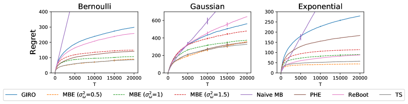
Figure 1: Simulation results under MAB. The error bars indicate the standard errors, which may not be visible when the width is small.

6.1 MAB Simulation

We first experiment with simulated MAB instances. The goal is to (i) further validate our theoretical findings, (ii) check whether MBE can yield comparable performance with standard methods, and (iii) study the robustness and adaptivity of MBE. We also experimented with linear bandits and the main findings are similar. To save space, we defer its results to Appendix LABEL:sec:results_LB.

We compare MBE with TS (Thompson, 1933), PHE (Kveton et al., 2019a), ReBoot (Wang et al., 2020), and GIRO (Kveton et al., 2019c). The last three algorithms are the existing bootstrap- or perturbation-type algorithms reviewed in Section 2. Specifically, PHE explores by perturbing observed rewards with additive noise, without leveraging the intrinsic uncertainly in the data, ReBoot explores by perturbing the residuals of the rewards observed for each arm, and GIRO re-samples observed data points. In all experiments below, the weights of MBE are sampled from $\mathcal{N}(1,\sigma_{\omega}^{2})$ . We fix $\lambda=0.5$ and run MBE with three different values of $\sigma_{\omega}^{2}$ as $0.5,1$ and $1.5$. We also compare with the naive adaption of multiplier bootstrap (i.e., no pseudo-rewards; denoted as Naive MB). We run Algorithm 2 with $B=50$ replicates.

We first study $10$-armed bandits, where the mean reward of each arm is independently sampled from $\text{Beta}(1,8)$. We consider three reward distributions, including Bernoulli, Gaussian, and exponential. For Gaussian MAB, the reward noise is sampled from $\mathcal{N}(0,1)$. The other two distributions are determined by their means. For TS, we always use the correct reward distribution class and its conjugate prior. The prior mean and variance are calibrated using the true model. Therefore, we use TS as a strong and standard baseline. For GIRO and ReBoot, we use the default implementations as they work well. For PHE, the original paper adds Bernoulli perturbation since it only studies bounded reward distributions. We extend PHE by sampling additive noise from the same distribution family as the true rewards, as did in Wu et al. (2022). GIRO, ReBoot and PHE all have one tuning parameter that control the degree of exploration. We tune these hyper-parameters over $\{2^{k-4}\}_{k=0}^{6}$, and report the best performance of each method. Without tuning, these algorithms generally do not perform well using the hyper-parameters suggested in the original papers, due to the differences in settings. We tuned Naive MB as well.

Results. Results over $100$ runs are displayed in Figure 1. Our findings can be summarized as follows. First, without knowledge of the problem settings (e.g., the reward distribution family and its parameters, and the prior distribution) and without heavy tuning, MBE performs favorably and close to TS. Second, pseudo-rewards are indeed important in exploration, otherwise the algorithm suffers a linear regret. Third, MBE has a stable performance with different $\sigma_{\omega}$ (note that other methods are tuned for their best performance). This is thanks to the data-driven nature of MBE. Finally, the other three general-purpose exploration strategies perform reasonably after tuning, as expected. However, GIRO is computationally intense. For example, in Gaussian bandits, the time cost for GIRO is $2$ minutes while all the other algorithms can complete within $10$ seconds. The computational burden is due to the limitation of non-parametric bootstrap (see Section 4.3). ReBoot also performs reasonably, yet by design it is not easy to extend it to many more complex problems (e.g., problems in Section 6.2).

Adaptivity. PHE relies on sampling additive noise from an appropriate distribution, and TS has similar dependency. In the results above, we provide auxiliary information about the environment to them and need to modify their implementation in different setups.  In contrast, MBE automatically adapts to these problems. As argued in Section 2, one main advantage of MBE over them is its adaptiveness. To see this, we consider the following procedure: we run the Gaussian versions of TS and PHE in Bernoulli MAB, and run their Bernoulli versions in Gaussian MAB. We also run MBE with $\sigma_{\omega}^{2}=0.5$. MBE does not require any modifications across the two problems. The results presented in Figure 2 clearly demonstrate that MBE adapts to reward distributions.

Similarly, we also studied the adaptivity of these methods against the reward distribution scale (the standard deviation of the Gaussian noise, $\sigma$) and the task distribution (we sample the mean rewards from $\text{Beta}(\alpha,8)$ and vary the parameter $\alpha$). For all settings, we use the algorithms tuned for Figure 1. We observe that, MBE shows impressive adaptiveness, while PHE and TS may not perform well when the environment is not close to the one they are tuned for. Recall that, in real applications, heavy tuning is not possible without ground truths. This demonstrates the adaptivity of MBE, as a data-driven exploration strategy.

Additional results. In Appendix LABEL:sec:results_robust_lam, we also try different values of $\lambda$ and $B$ for MBE. We also repeat the main experiment with $K=25$. Our main observations above still hold and MBE is relatively robust to these tuning parameters.

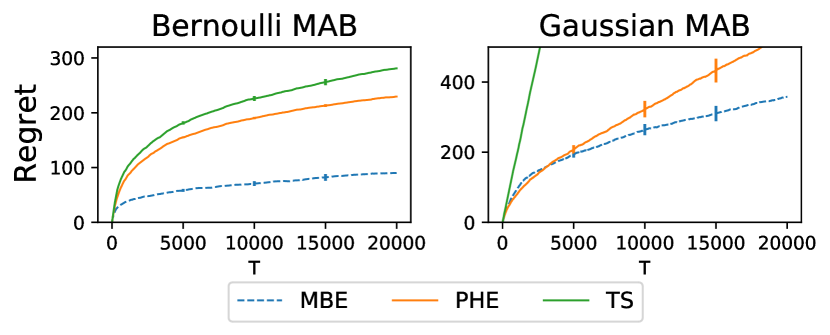
Figure 2: Robust results against the reward distribution class.

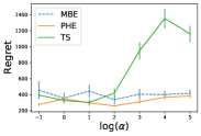
(a) Trend with $\alpha$

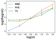
(b) Trend with $\sigma$

Figure 3: Results with different reward variances and task distributions. For the x-axis in both figures and the y-axis in the second one, we plot at the logarithmic scale for better visualization.

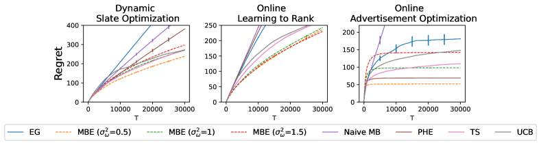
Figure 4: Real data results for three structured bandit problems that need domain-specific models.

6.2 Real data applications

The main advantage of MBE is that it easily generalizes to complex models. In this section, we use real datasets to study this property. Our goal is to investigate that, without problem-specific algorithm design and without heavy tuning, whether MBE can achieve comparable performance with strong problem-specific baselines proposed in the literature.

We study the three problems considered in Wan et al. (2022), including cascading bandits for online learning to rank (Kveton et al., 2015), combinatorial semi-bandits for online combinatorial optimization (Chen et al., 2013), and multinomial logit (MNL) bandits for dynamic slate optimization (Agrawal et al., 2017, 2019). All these are practical and important problems in real life. Yet, these domain models all have unique structures and require a case-by-case algorithm design. For example, the rewards in MNL bandits follow multinomial distributions that have complex dependency with the pulled arms. To derive the posterior or confidence bound, one has to use a delicately designed epoch-type procedure (Agrawal et al., 2019).

We compared MBE with state-of-the-art baselines in the literature, including TS-Cascade (Zhong et al., 2021) and CascadeKL-UCB (Kveton et al., 2015) for cascading bandits, CUCB (Chen et al., 2016) and CTS (Wang & Chen, 2018) for semi-bandits, and MNL-TS (Agrawal et al., 2017) and MNL-UCB (Agrawal et al., 2019) for MNL bandits. To save space, we denote the TS-type algorithms by TS and UCB-type ones by UCB. We also study PHE and $\epsilon$-greedy (EG) as two other general-purpose exploration strategies.

We use the three datasets studied in Wan et al. (2022). Specifically, we use the Yelp rating dataset (Zong et al., 2016) to recommend and rank $K$ restaurants, use the Adult dataset (Dua & Graff, 2017) to send advertisements to $K/2$ men and $K/2$ women (a combinatorial semi-bandit problem with continuous rewards), and use the MovieLens dataset (Harper & Konstan, 2015) to display $K$ movies. In our experiments, we fix $K=4$ and randomly sample $30$ items from the dataset to choose from. We provide a summary of these datasets and problems in Appendix LABEL:sec:exp_details, and refer interested readers to Wan et al. (2022) and references therein for more details.

For the baseline methods, as in Section 6.1, we either use the default hyperparameters in Wan et al. (2022) or tune them extensively and present their best performance. For EG, we set the exploration rate $\epsilon_{t}=\min(1,a/2\sqrt{t})$ with tuning parameter $a$. For MBE, with every bootstrap sample, we estimate the reward model via maximum weighted likelihood estimation, which yields nice closed-form solution that allows online updating in all three problems. The other implementation details are similar to Section 6.1.

We present the results in Figure 4. The overall findings are consistent with simulation. First, without any additional derivations or algorithm design, MBE matches the performance of problem-specific algorithms. Second, pseudo-rewards are important to guarantee sufficient exploration, and naively applying multiplier bootstrap may fail. Third, MBE has relatively stable performance with $\sigma_{\omega}$, as its exploration is mostly data-driven. In contrast, we found that the hyper-parameters of PHE and EG have to be carefully tuned, due to that they rely on externally added perturbation or forced exploration. For example, the best parameters for EG are $a=5$, $0.1$ and $0.5$ in three problems. Finally, we observe that PHE does not perform well in MNL and cascading bandits, where the outcomes are binary. From a closer look, we find one possible reason: the response rates (i.e., the probabilities for the binary outcome to be $1$) in the two datasets are low, so PHE introduces too much (additive) noise for exploration purpose, which slows down the estimation convergence.

7 Conclusion

In this paper, we propose a new bandit exploration strategy, Multiplier Bootstrap-based Exploration (MBE). The main advantage of MBE is its generality: for any reward model that can be estimated via weighted loss minimization, the idea of MBE is applicable and requires minimal efforts on derivation or implementation of the exploration mechanism. As a data-driven method, MBE also shows nice adaptivity. We prove near-optimal regret bounds for MBE in the sub-Gaussian MAB setup, which is more general compared with other bootstrap-based bandit papers. Numerical experiments demonstrate that MBE is general, efficient, and adaptive.

There are a few meaningful future extensions. First, the regret analysis for MBE (and more generally, other bootstrap-based bandit methods) in more complicated setups would be valuable. Second, adding pseudo-rewards at every round is needed for the analysis. We hypothesize that there exists a more adaptive way of adding them. Last, the practical implementation of MBE relies on an ensemble of models to approximate the bootstrap distribution and the online regression oracle to update the model estimation. Our numerical experiments show that such an approach works well empirically, but it would be still meaningful to have more theoretical understanding.

Appendix A A Additional Method Details

A.1 MBE for MAB

In this section, we present the concrete form of MBE when being applied to MAB. Recall that ${\bm{x}}_{t}$ is null, $A_{t}\in[K]$, and $r_{k}$ is the mean reward of the $k$-th arm. We define $f({\bm{x}}_{t},A_{t};{\bm{r}})=r_{A_{t}}$, where the parameter vector ${\bm{r}}=(r_{1},\dots,r_{K})^{\top}$. We define the loss function as

$$\frac{1}{t^{\prime}}\sum_{t=1}^{t^{\prime}}\omega_{t}(r_{A_{t}}-R_{t})^{2}.$$

The solution is then $(\widehat{r}_{1},\dots,\widehat{r}_{K})^{\top}$ with $\widehat{r}_{k}=(\sum_{t:A_{t}=k}\omega_{t})^{-1}\sum_{t:A_{t}=k}\omega_{t}R_{t}$, i.e., the arm-wise weighted average. After adding the pseudo rewards, we can give algorithm for MAB in Algorithm LABEL:alg:MBTS-MAB-2.

Next, we provide intuitive explanation on why Algorithm LABEL:alg:MBTS-MAB-2 works. Indeed, denote $s:=|\mathcal{H}_{k,T}|$, where $\mathcal{H}_{k,T}$ is the set of observed rewards for the $k$-th arm up to round $T$. Let $R_{k,l}$ be the $l$-th element in $\mathcal{H}_{k,T}$. Then

$$\overline{Y}_{k,s} =\frac{\sum_{i=1}^{s}\omega_{i}R_{k,i}+\lambda\sum_{i=1}^{s}\omega_{i}^{\prime}}{\sum_{i=1}^{s}\omega_{i}+\lambda\sum_{i=1}^{s}\omega_{i}^{\prime}+\lambda\sum_{i=1}^{s}\omega_{i}^{\prime\prime}}$$

$$=\frac{s^{-1}\sum_{i=1}^{s}\omega_{i}(R_{k,i}-\mu_{k})+s^{-1}\sum_{i=1}^{s}(\omega_{i}-1)+\lambda s^{-1}\sum_{i=1}^{s}(\omega_{i}^{\prime}-1)+\mu_{k}+\lambda}{s^{-1}\sum_{i=1}^{s}(\omega_{i}-1)+\lambda s^{-1}\sum_{i=1}^{s}(\omega_{i}^{\prime}-1)+\lambda s^{-1}\sum_{i=1}^{s}(\omega_{i}^{\prime\prime}-1)+1+2\lambda}\,\xlongrightarrow{\mathbb{P}}\,\frac{\mu_{k}+\lambda}{1+2\lambda}$$

by using the law of large numbers. Then, by Slutsky’s theorem,

$$\sqrt{s}\left[\overline{Y}_{k,s}-\frac{\mu_{k}+\lambda}{1+2\lambda}\right]=\frac{1}{1+2\lambda}\left[\frac{1}{\sqrt{s}}\sum_{i=1}^{s}\omega_{i}(R_{k,i}-\mu_{k})+\frac{1}{\sqrt{s}}\sum_{i=1}^{s}(\omega_{i}-1)+\frac{\lambda}{\sqrt{s}}\sum_{i=1}^{s}(\omega_{i}^{\prime}-1)\right]+o_{p}(1)$$

will weakly converge to a mean-zero Gaussian distribution $\mathcal{N}\left(0,\frac{\sigma_{k}^{2}+2}{(1+2\lambda)^{2}}\sigma_{\omega}^{2}\right)$. Therefore, our algorithm preserves the order of the arms for any $\lambda>0$.

Data: number of arms $K$, multiplier weight distribution $\rho(\omega)$, tuning parameter $\lambda$

Set $\mathcal{H}_{k}=\{\}$ be the history of the arm $k$ and $\overline{Y}_{k}=+\infty,\forall k\in[K]$

for $t=1,\dots,T$ do

3       Pull $A_{t}=\operatorname*{arg\,max}_{k\in[K]}\overline{Y}_{k}$ (break tie randomly), Observe reward $R_{t}$ Set $\mathcal{H}_{k}=\mathcal{H}_{k}\cup\{R_{t}\}$ for $k=1,\dots,K$ do

4             if $|\mathcal{H}_{k}|>0$ then

5                   Sample the multiplier weights $\{\omega_{l},\omega^{\prime}_{l},\omega^{\prime\prime}_{l}\}_{l=1}^{|\mathcal{H}_{k}|}\sim\rho(\omega)$. Update the mean reward

$$\overline{Y}_{k}=\left(\sum_{\ell=1}^{|\mathcal{H}_{k}|}(\omega_{\ell}\cdot R_{k,\ell}+\omega_{\ell}^{\prime}\cdot 1\times\lambda+\omega_{\ell}^{\prime\prime}\cdot 0\times\lambda)\right)/\left(\sum_{\ell=1}^{|\mathcal{H}_{k}|}(\omega_{\ell}+\lambda\omega_{\ell}^{\prime}+\lambda\omega_{\ell}^{\prime\prime})\right),$$

where $R_{k,l}$ is the $l$-th element in $\mathcal{H}_{k}$.

6             end if

7            

8       end for

9

References

- Agrawal et al. (2017) Agrawal, S., Avadhanula, V., Goyal, V., and Zeevi, A. Thompson sampling for the mnl-bandit. arXiv preprint arXiv:1706.00977, 2017.
- Agrawal et al. (2019) Agrawal, S., Avadhanula, V., Goyal, V., and Zeevi, A. Mnl-bandit: A dynamic learning approach to assortment selection. Operations Research, 67(5):1453–1485, 2019.
- Auer et al. (2002) Auer, P., Cesa-Bianchi, N., and Fischer, P. Finite-time analysis of the multiarmed bandit problem. Machine learning, 47(2):235–256, 2002.
- Bietti et al. (2021) Bietti, A., Agarwal, A., and Langford, J. A contextual bandit bake-off. J. Mach. Learn. Res., 22:133–1, 2021.
- Chapelle & Zhang (2009) Chapelle, O. and Zhang, Y. A dynamic bayesian network click model for web search ranking. In Proceedings of the 18th international conference on World wide web, pp. 1–10, 2009.
- Chen et al. (2013) Chen, W., Wang, Y., and Yuan, Y. Combinatorial multi-armed bandit: General framework and applications. In International Conference on Machine Learning, pp. 151–159. PMLR, 2013.
- Chen et al. (2016) Chen, W., Wang, Y., Yuan, Y., and Wang, Q. Combinatorial multi-armed bandit and its extension to probabilistically triggered arms. The Journal of Machine Learning Research, 17(1):1746–1778, 2016.
- Dua & Graff (2017) Dua, D. and Graff, C. UCI machine learning repository, 2017. URL http://archive.ics.uci.edu/ml.
- Durand et al. (2018) Durand, A., Achilleos, C., Iacovides, D., Strati, K., Mitsis, G. D., and Pineau, J. Contextual bandits for adapting treatment in a mouse model of de novo carcinogenesis. In Machine learning for healthcare conference, pp. 67–82. PMLR, 2018.
- Eckles & Kaptein (2014) Eckles, D. and Kaptein, M. Thompson sampling with the online bootstrap. arXiv preprint arXiv:1410.4009, 2014.
- Efron (1992) Efron, B. Bootstrap methods: another look at the jackknife. In Breakthroughs in statistics, pp. 569–593. Springer, 1992.
- Elmachtoub et al. (2017) Elmachtoub, A. N., McNellis, R., Oh, S., and Petrik, M. A practical method for solving contextual bandit problems using decision trees. arXiv preprint arXiv:1706.04687, 2017.
- Filippi et al. (2010) Filippi, S., Cappe, O., Garivier, A., and Szepesvári, C. Parametric bandits: The generalized linear case. Advances in Neural Information Processing Systems, 23, 2010.
- Hao et al. (2019) Hao, B., Abbasi Yadkori, Y., Wen, Z., and Cheng, G. Bootstrapping upper confidence bound. Advances in Neural Information Processing Systems, 32, 2019.
- Harper & Konstan (2015) Harper, F. M. and Konstan, J. A. The movielens datasets: History and context. Acm transactions on interactive intelligent systems (tiis), 5(4):1–19, 2015.
- Kveton et al. (2015) Kveton, B., Szepesvari, C., Wen, Z., and Ashkan, A. Cascading bandits: Learning to rank in the cascade model. In International Conference on Machine Learning, pp. 767–776. PMLR, 2015.
- Kveton et al. (2019a) Kveton, B., Szepesvári, C., Ghavamzadeh, M., and Boutilier, C. Perturbed-history exploration in stochastic multi-armed bandits. In Proceedings of the 28th International Joint Conference on Artificial Intelligence, pp. 2786–2793, 2019a.
- Kveton et al. (2019b) Kveton, B., Szepesvari, C., Ghavamzadeh, M., and Boutilier, C. Perturbed-history exploration in stochastic linear bandits. arXiv preprint arXiv:1903.09132, 2019b.
- Kveton et al. (2019c) Kveton, B., Szepesvari, C., Vaswani, S., Wen, Z., Lattimore, T., and Ghavamzadeh, M. Garbage in, reward out: Bootstrapping exploration in multi-armed bandits. In International Conference on Machine Learning, pp. 3601–3610. PMLR, 2019c.
- Kveton et al. (2020a) Kveton, B., Zaheer, M., Szepesvari, C., Li, L., Ghavamzadeh, M., and Boutilier, C. Randomized exploration in generalized linear bandits. In International Conference on Artificial Intelligence and Statistics, pp. 2066–2076. PMLR, 2020a.
- Kveton et al. (2020b) Kveton, B., Zaheer, M., Szepesvari, C., Li, L., Ghavamzadeh, M., and Boutilier, C. Randomized exploration in generalized linear bandits. In International Conference on Artificial Intelligence and Statistics, pp. 2066–2076. PMLR, 2020b.
- Lattimore & Szepesvári (2020) Lattimore, T. and Szepesvári, C. Bandit algorithms. Cambridge University Press, 2020.
- Li et al. (2017) Li, L., Lu, Y., and Zhou, D. Provably optimal algorithms for generalized linear contextual bandits. In International Conference on Machine Learning, pp. 2071–2080. PMLR, 2017.
- Lu & Van Roy (2017) Lu, X. and Van Roy, B. Ensemble sampling. Advances in neural information processing systems, 30, 2017.
- Osband & Van Roy (2015) Osband, I. and Van Roy, B. Bootstrapped thompson sampling and deep exploration. arXiv preprint arXiv:1507.00300, 2015.
- Osband et al. (2019) Osband, I., Van Roy, B., Russo, D. J., Wen, Z., et al. Deep exploration via randomized value functions. J. Mach. Learn. Res., 20(124):1–62, 2019.
- Phan et al. (2019) Phan, M., Abbasi Yadkori, Y., and Domke, J. Thompson sampling and approximate inference. Advances in Neural Information Processing Systems, 32, 2019.
- Qin et al. (2022) Qin, C., Wen, Z., Lu, X., and Roy, B. V. An analysis of ensemble sampling. In Oh, A. H., Agarwal, A., Belgrave, D., and Cho, K. (eds.), Advances in Neural Information Processing Systems, 2022. URL https://openreview.net/forum?id=c6ibx0yl-aG.
- Riquelme et al. (2018) Riquelme, C., Tucker, G., and Snoek, J. Deep bayesian bandits showdown: An empirical comparison of bayesian deep networks for thompson sampling. arXiv preprint arXiv:1802.09127, 2018.
- Shen et al. (2015) Shen, W., Wang, J., Jiang, Y.-G., and Zha, H. Portfolio choices with orthogonal bandit learning. In Twenty-fourth international joint conference on artificial intelligence, 2015.
- Tang et al. (2015) Tang, L., Jiang, Y., Li, L., Zeng, C., and Li, T. Personalized recommendation via parameter-free contextual bandits. In Proceedings of the 38th international ACM SIGIR conference on research and development in information retrieval, pp. 323–332, 2015.
- Tang et al. (2021) Tang, Q., Xie, H., Xia, Y., Lee, J., and Zhu, Q. Robust contextual bandits via bootstrapping. In Proceedings of the AAAI Conference on Artificial Intelligence, volume 35, pp. 12182–12189, 2021.
- Thompson (1933) Thompson, W. R. On the likelihood that one unknown probability exceeds another in view of the evidence of two samples. Biometrika, 25(3-4):285–294, 1933.
- Van Der Vaart & Wellner (1996) Van Der Vaart, A. W. and Wellner, J. A. Weak convergence. In Weak convergence and empirical processes, pp. 16–28. Springer, 1996.
- Vaswani et al. (2018) Vaswani, S., Kveton, B., Wen, Z., Rao, A., Schmidt, M., and Abbasi-Yadkori, Y. New insights into bootstrapping for bandits. arXiv preprint arXiv:1805.09793, 2018.
- Wan et al. (2022) Wan, R., Ge, L., and Song, R. Towards scalable and robust structured bandits: A meta-learning framework. arXiv preprint arXiv:2202.13227, 2022.
- Wang et al. (2020) Wang, C.-H., Yu, Y., Hao, B., and Cheng, G. Residual bootstrap exploration for bandit algorithms. arXiv preprint arXiv:2002.08436, 2020.
- Wang & Chen (2018) Wang, S. and Chen, W. Thompson sampling for combinatorial semi-bandits. In International Conference on Machine Learning, pp. 5114–5122. PMLR, 2018.
- Watkins (1989) Watkins, C. J. C. H. Learning from delayed rewards. 1989.
- Wen et al. (2015) Wen, Z., Kveton, B., and Ashkan, A. Efficient learning in large-scale combinatorial semi-bandits. In International Conference on Machine Learning, pp. 1113–1122. PMLR, 2015.
- Wu et al. (2022) Wu, S., Wang, C.-H., Li, Y., and Cheng, G. Residual bootstrap exploration for stochastic linear bandit. arXiv preprint arXiv:2202.11474, 2022.
- Zhang & Chen (2021) Zhang, H. and Chen, S. Concentration inequalities for statistical inference. Communications in Mathematical Research, 37(1):1–85, 2021.
- Zhang & Wei (2022) Zhang, H. and Wei, H. Sharper sub-weibull concentrations. Mathematics, 10(13):2252, 2022.
- Zhong et al. (2021) Zhong, Z., Chueng, W. C., and Tan, V. Y. Thompson sampling algorithms for cascading bandits. Journal of Machine Learning Research, 22(218):1–66, 2021.
- Zhou et al. (2020) Zhou, D., Li, L., and Gu, Q. Neural contextual bandits with ucb-based exploration. In International Conference on Machine Learning, pp. 11492–11502. PMLR, 2020.
- Zhou et al. (2017) Zhou, Q., Zhang, X., Xu, J., and Liang, B. Large-scale bandit approaches for recommender systems. In International Conference on Neural Information Processing, pp. 811–821. Springer, 2017.
- Zong et al. (2016) Zong, S., Ni, H., Sung, K., Ke, N. R., Wen, Z., and Kveton, B. Cascading bandits for large-scale recommendation problems. arXiv preprint arXiv:1603.05359, 2016.