Contrastive Learning with Consistent Representations

Abstract

Contrastive learning demonstrates great promise for representation learning. Data augmentations play a critical role in contrastive learning by providing informative views of the data without needing the labels. However, the performance of the existing works heavily relies on the quality of the employed data augmentation (DA) functions, which are typically hand picked from a restricted set of choices. While exploiting a diverse set of data augmentations is appealing, the intricacies of DAs and representation learning may lead to performance degradation. To address this challenge and allow for a systemic use of large numbers of data augmentations, this paper proposes Contrastive Learning with Consistent Representations (CoCor). At the core of CoCor is a new consistency measure, DA consistency, which dictates the mapping of augmented input data to the representation space such that these instances are mapped to optimal locations in a way consistent to the intensity of the DA applied. Furthermore, a data-driven approach is proposed to learn the optimal mapping locations as a function of DA while maintaining a desired monotonic property with respect to DA intensity. The proposed techniques give rise to a semi-supervised learning framework based on bi-level optimization, achieving new state-of-the-art results for image recognition.

1 Introduction

Data augmentation is widely used in supervised learning for image recognition, achieving excellent results on popular datasets like MNIST, CIFAR-10/100, and ImageNet [7, 22, 23, 26, 16]. AutoAugment [8] and RandAugment [9] use strong augmentations composed of a combination of different transformations. It has been shown that these manually designed data augmentations can effectively increase the amount of training data and enhance the model’s ability to capture the invariance of the training data, thereby boosting supervised training performance.

Data augmentation (DA) is also a key component in recent semi-supervised learning techniques based on contrastive learning [5]. A base encoder that learns good latent representations of the input data is trained with a contrastive loss. The contrastive loss is reflective of the following: in the latent space a pair of two views of a given data example transformed by two different data augmentation functions are correlated (similar) while transformed views of different input examples are dissimilar. The quality of the encoder trained using unlabeled data as such is essential to the overall contrastive learning performance, and is contingent upon the employed data augmentations.

[27] interprets the minimization of the contrastive loss is to achieve alignment and uniformity of the learned representations. To learn powerful and transferable representations, many studies have aimed at improving contrastive learning by choosing proper data augmentations [5, 25, 11] have shown that combining different augmentations with a proper magnitude may improve performance. In these works, data augmentations are restricted to be a random composition of four or five types of augmentations with a very limited range of magnitude. To further improve contrastive learning in downstream tasks, PIRL [20] adopts two additional data augmentations, SwAV [4] introduced multiple random resized-crops to provide the encoder with more views of data and CLSA [28] adopts combinations of stronger augmentations.

While exploiting a diverse set of data augmentations is appealing, thus far, there does not exist a systematic approach for incorporating a large number of augmentations for contrastive learning. Importantly, the intricacies of data augmentation and representation learning may result in performance degradation if data augmentation functions are not properly chosen and used. To address the above challenges, this paper proposes Contrastive Learning with Consistent Representations (CoCor). First, we define a set of composite augmentations, denoted by $\bm{A}$ and composed by combining multiple basic augmentations. We represent each composite augmentation using a composition vector that encodes the types and numbers of basic augmentations used and their augmentation magnitude. A large number of diverse augmentations can be drawn from this composite set $\bm{A}$ with widely varying transformation types and overall strength.

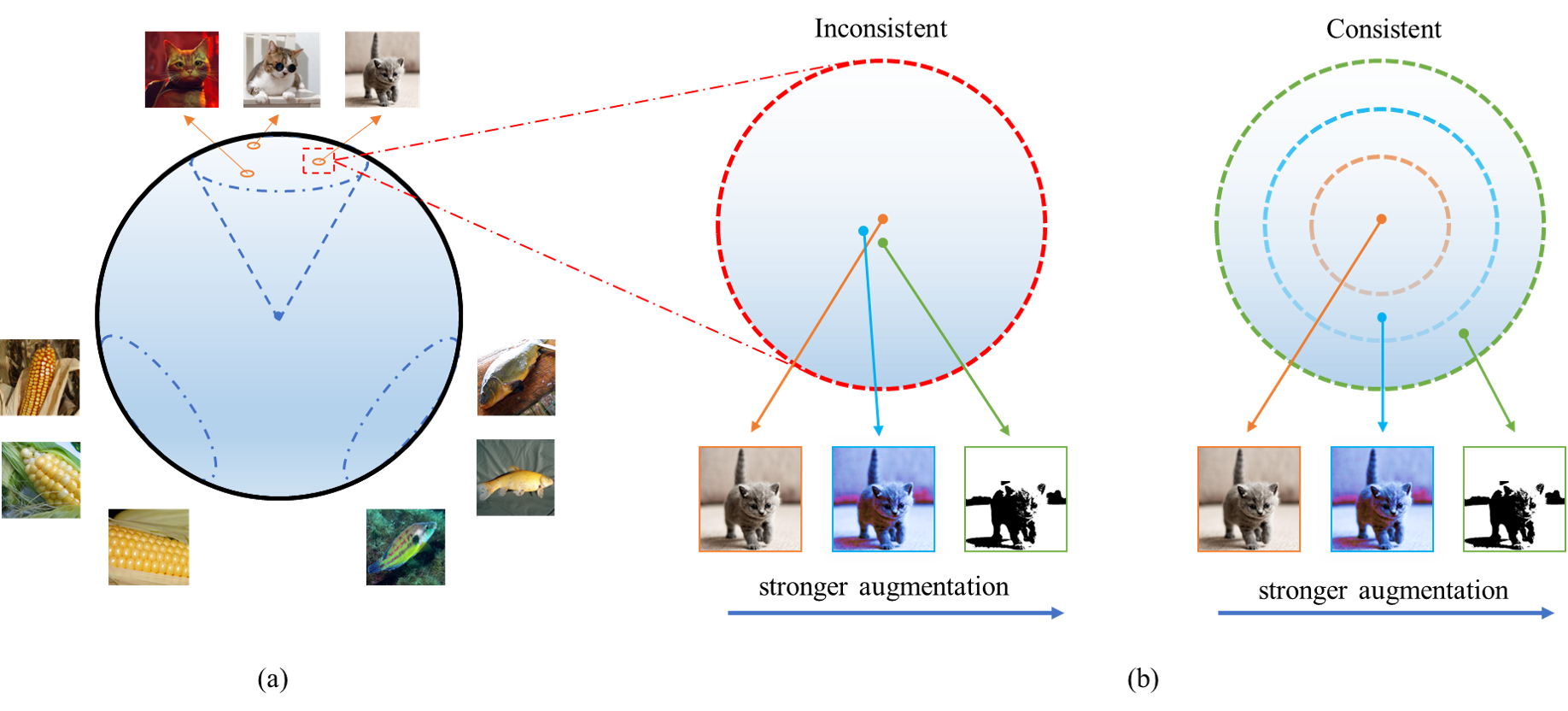
Critically, we propose a notion of consistency for data augmentations, called DA consistency, which imposes a desiring property on the latent representations of views produced by different composite data augmentations. For a given input example, a stronger data augmentation shall push its latent-space view further away from the latent representation of the original example. That is, the latent-space similarity between the transformed view and the original input decreases with the strength of the data augmentation, a very desiring characteristic, as illustrated in Fig. 1(b). In other words, a base encoder that does not satisfy the above property is deemed inconsistent from a data augmentation point of view. We consequently propose to add a new consistency loss to impose DA consistency on the base encoder. Different from the contrastive loss that is agnostic to the type and overall strength of employed data augmentations  [5, 25, 11], our consistency loss places additional finer-grained constraints on the encoder learning such that the resulted latent-space views are consistent with the strength of data augmentations applied. Enforcing DA consistency is key to circumventing inconsistencies among diverse data augmentations, which may result in performance degradation.

Figure 1: (a): Contrastive learning aims at learning well-clustered representations on the latent hypersphere [27]. (b)-Left: Encoder trained with standard contrastive loss is inconsistent since different views of an instance are encouraged to be represented samely in the feature space, regardless of the actual difference between them. (b)-Right: For a consistent encoder, the latent view of stronger augmented data should be further away from the latent view of the raw data.

The proposed consistency loss is defined upon the optimal similarity between the latent-space representations of an input example and a transformed view, which is a function of the strength of the composite data augmentation. However, this optimal similarity is not known a prior. To cope with this difficulty, we take a data-driven approach to train a black-box neural network that maps from the composition vector of each data augmentation to the desired similarity using bi-level optimization. Recognizing that the similarity monotonically decreases with the strength of augmentation, we define and impose a partial monotonicity constraint to the black-box neural network such that strictly stronger composition data augmentations correspond to a strictly smaller valued similarity.

The main contributions to contrastive learning from this paper are as follows:

• Systematically explore a large set of diverse composite data augmentations for which we define a partial monotonicity concept.

• Propose a new notion of consistency called DA consistency for data augmentation, quantifying the monotonic dependency of the latent-space similarity between an input example and its transformed view as a function of the strength of the augmentation.

• Introduce a new consistency loss for training the base encoder towards satisfying DA consistency and for making use of diverse augmentations without inconsistency-induced performance loss.

• Propose a data-driven approach to learn the desired latent-space similarities with properly defined partial monotonicity based on bi-level optimization.

The proposed techniques give rise to a semi-supervised learning framework based on bi-level optimization, achieving new state-of-the-art results for image recognition.

2 Related works

2.1 Contrastive Learning

Recently, a lot of contrastive learning methods have shown impressive results in visual representation learning. SimCLR [5] takes advantage of manually designed data augmentation to produce a pool of negative and positive data pairs in minibatches. A momentum updated encoder and a large representations memory bank were introduced to further improve the performance in MOCO [11]. Alignment and uniformity [27] were introduced to describe the quality of representations. It was shown that by minimizing contrastive loss alignment and uniformity of features can be asymptotically achieved.

2.2 Data Augmentation

In supervised deep learning, data augmentation has already been applied to natural image datasets while training, which helps improve the generalization and robustness of learnt models. Works like AutoAugment [8] and RandAugment [9] adopted combinations of various transformations to produce strong data augmentation. In self-supervised learning [5, 25, 11], data augmentations are carefully designed by sampling from a highly restricted set of augmentations to maintain identity of instances and avoid noise. SwAV [4] used multiple random resized-crops to produce more views of data. CLSA [28] utilized combinations of augmentations as stronger augmentation, in which the encoder is trained to match the distribution of the representations of weakly and strongly augmented instances.

2.3 Bi-level Optimization

In deep learning, bi-level optimization is used to adaptively adjust the learning rate during training [1]. DARTS [19] proposed an approach of architecture search based on bi-level optimization. In semi-supervised and self-supervised learning, Meta Pseudo Labels [21] adopted bi-level optimization to simultaneously update a student model and a teacher model. JOAO [30] used bi-level optimization in adaptively adjusting data augmentation applied to graph-structured data.

3 Preliminaries

3.1 Contrastive Learning with Memory

The goal of contrastive representation learning is to learn a powerful encoder parameterized by $\bm{\theta_{e}}$ that maps an input data $\bm{x}\in\mathbb{R}^{n}$ to an $\ell_{2}$ normalized feature vector $\bm{z}$ of dimension $m$, i.e., $f_{\bm{\theta_{e}}}(\cdot):\mathbb{R}^{n}\to\mathcal{S}^{m-1}$. The encoder is trained by minimizing a contrastive loss. Specifically, it defines two different augmented versions of the same input example as a positive pair, which are expected to have similar representations in the feature space. Meanwhile, the encoder shall be trained to discriminate any two instances augmented from different input examples, i.e., a negative pair, in the latent feature space. Empirically, a queue $\mathcal{Q}$ of negative embeddings is maintained for forming negative pairs with augmented data from each minibatch $\mathcal{B}$. In this paper, we consider the wide adopted loss that has been shown to be effective in representation learning [5, 11, 24]:

$$\begin{split}\mathcal{L}_{\text{contrast}}=\mathbb{E}_{i\in\mathcal{B}}[-\log\frac{e^{\bm{z}_{i}^{T}\bm{z}_{i}^{+}/\tau}}{e^{\bm{z}_{i}^{T}\bm{z}_{i}^{+}/\tau}+\sum_{z_{j}\in\mathcal{Q}}e^{\bm{z}_{i}^{T}\bm{z}_{j}/\tau}}]\end{split}$$ (1)

where $\bm{z}_{i}$ and $\bm{z}_{i}^{+}$ denote the representations of a positive pair, $\bm{z}_{i}$ and $\bm{z}_{j}$ are representations of a negative pair. $\bm{z}^{T}\bm{z}$ denotes the cosine similarity of feature vectors, which is scaled by temperature $\tau$.

3.2 Inconsistency in Contrastive Learning

Data augmentation plays a pivotal role in contrastive learning and needs to be carefully designed to maintain the latent structure of the original data. Despite that a variety of augmentations have been successfully applied to supervised settings, contrastive learning benefits from diverse augmentations to a lesser degree, and only a subset of "weak" augmentations have been empirically shown to be effective. For instance, in the popular contrastive learning framework of [5, 11, 6, 25], the adopted data augmentations are limited to a combination of three to five types of basic transformations, which are chosen empirically according to the experience. Adding to or removing from this pre-selected basic transformations can deteriorate the performance, a phenomenon that is not well understood. Moreover, although a few works have attempted to introduce “stronger"

augmentations[4, 28, 20], there still lacks a systematic view of how augmentations with a widely varying strength affect the learning process and how to leverage a larger set of diverse augmentations to improve, as opposed to, degrade the performance .

Our key observation is that the vanilla contrastive learning framework[5, 11] does not imply data augmentation (DA) consistency, a key property proposed by this work, which should be maintained during contrastive learning. Without the consistency in place, the optimized encoder simply pulls positive pairs to the same position in the latent space $\mathcal{S}^{m-1}$, regardless of the actual difference between them. However, a weakly augmented view and a strongly augmented view of an input example do not necessarily share the same latent structure, and it may be desirable to encode them to different regions in the feature space. An illustrated example is shown in Fig. 1 (b). In this case, the encoder that tries to pull the positive pairs together learns an incorrect latent representation. We refer to this phenomenon as data augmentation inconsistency in contrastive learning.

To prevent this inconsistency, the encoder should be trained to not only cluster positive pairs together, but also map them to their respective optimal location on $\mathcal{S}^{m-1}$, based on the strength of the applied augmentations. We thereby define this property as data augmentation consistency, shortly DA consistency, an additional constraint for contrastive learning. The proposed DA consistency takes into account the critical role played by the augmentation strength in the learning process, removes potential inconsistencies across different augmentations, and facilities effective use of large numbers of diverse augmentations.

4 Method

4.1 Composite Augmentations

Definition 4.1 (Composite Augmentations).

Given a set of $k$ basic augmentations $\bm{T}=\left\{T_{1},T_{2}\cdots T_{k}\right\}$, a composite augmentation with a length of $l$, namely, $A^{l}$ is defined as the composition of $l$ randomly sampled augmentations from $\bm{T}$:

$$\quad\ A^{l}=T^{1}\circ T^{2}\circ\cdots T^{l}$$ (2)

$$\text{where}\ \ T^{i}\in\bm{T},\ i={1,2\cdots l}$$

We denote the set that contains all composite augmentations with a length of $l$ by $\bm{A}^{l}$, and denote the set that contains all composite augmentations with different lengths by $\bm{A}=\bm{A}^{1}\cup\bm{A}^{2}\cdots$. Empirical studies showed that the ordering of the basic augmentations in a composite augmentation does not have a significant impact on performance. To simplify the discussion, we do not consider the effect of the ordering of the basic transformations in each composite augmentation $A\in\bm{A}$ and hence assume that $A$ is order invariant, e.g., $T^{1}\circ T^{2}=T^{2}\circ T^{1}$. Thereby, we represent a composite augmentation with an unique composition vector.

Definition 4.2 (Composition Vector).

The composition vector of a composite augmentation $A^{l}$ is defined as a $k$ dimensional vector $\bm{V}(A^{l})\in{\mathbb{R}^{k}}$, where the $i_{th}$ entry $V_{i}$ is the number of times that the basic augmentation $T_{i}$ is used in $A^{l}$. Specifically, $\sum_{i=1}^{k}V_{i}=l$.

Given an encoder $f$, the location in $\mathcal{S}^{m-1}$ to which an encoded augmented view $A(\bm{x})$ is mapped can be characterized by the cosine similarity between $f(\bm{x})$ and $f(A(\bm{x}))$, which we define as latent deviation below.

Definition 4.3 (Latent Deviation).

Given a raw input example $\bm{x}$, an encoder $f$, and a composite augmentation $A\in\bm{A}$, the latent deviation $\Omega(\cdot;f,A)$ of $A(\bm{x})$ is defined as the cosine similarity between $\bm{x}$ and $A(\bm{x})$ in the latent space $\mathcal{S}^{m-1}$:

$$\Omega(\bm{x};f,A)=f(\bm{x})^{T}\cdot f(A(\bm{x})).$$ (3)

We assume that encoder $f$ maps its input to a normalized vector in the latent space.

4.2 Data Augmentation Consistency

Defining the aforementioned DA consistency in contrastive learning requires quantifying the strength of different augmentations and learning a mapping from the strength to the optimal mapped location in $\mathcal{S}^{m-1}$ with respect to a given raw input example $\bm{x}$. We specify a mapped latent space location using the corresponding latent deviation. To be DA consistent, latent deviations of different augmentations shall be monotonically decreasing with the augmentation strength.

However, a straightforward definition of augmentation strength is challenging. This is because that two composite augmentations may consist of different basic augmentation types and it is not immediately evident how to define and compare their strength levels. To tackle this problem, we take a black-box data-driven approach to directly learn a mapping $g^{*}$ that takes a composite augmentation as input and map it to the optimal mapped latent space location of the augmented view of each given raw input $\bm{x}$, relaxing the necessity of modeling the strength of different augmentations. Since a key objective of contrastive learning is to find an optimal encoder $f^{*}$ that delivers the best performance, the optimal mapped location outputted by mapping $g^{*}$ is specified as the corresponding latent deviation of an optimal encoder $f^{*}$.

Under this optimal $f^{*}$, the mapped latent space location $f(A(\bm{x}))$ in $\mathcal{S}^{m-1}$ corresponds to the optimal latent deviation. The optimal encoder $f^{*}$ is defined to be fully data-augmentation consistent, or fully DA consistent in short, and its latent derivation for any given composite augmentation is considered optimal. For other encoders that are not fully DA consistent, we further define DA consistency level, as the degree at which the learned representations are consistent in terms of data augmentation.

Definition 4.4 (Consistency Level).

Given an encoder $f$, a set of composite augmentation $\bm{A}$, a raw input $\bm{x}$, and a fully DA consistent encoder $f^{*}$, the DA consistency level (DACL) is define as:

$$\text{DACL}(\bm{x},f;f^{*},\bm{A})=\mathbb{E}_{A\sim\bm{A}}[\lvert\Omega(\bm{x};f,A)-\Omega(\bm{x};f^{*},A)\lvert]$$ (4)

DACL measures the level of consistency of a given encoder $f$ by comparing the latent deviation of the augmented view of $\bm{x}$ with the corresponding optimal latent deviation $\Omega(\bm{x};f^{*},A^{l})$ over all possible composite augmentations.

With DACL, an encoder that is not fully DA consistent can be trained to be more DA consistent by minimizing the consistency loss defined below:

$$\quad\mathcal{L}_{\text{consistent}}(\bm{\theta_{e}})$$ (5)

$$=\mathbb{E}_{\bm{x}\sim\mathcal{B}}[\text{DACL}(\bm{x},f;f^{*},\bm{A})]$$

$$=\mathbb{E}_{\bm{x}\sim\mathcal{B},A\sim\bm{A}}[\lvert\Omega(\bm{x};f,A)-\Omega(\bm{x};f^{*},A)\lvert]$$

where $\bm{\theta_{e}}$ is the parameter of the encoder $f$.

4.3 Learning Optimal Latent Deviations with a Partially Monotonic Neural Network

Improving the consistency of an encoder by minimizing the proposed consistency loss needs to determine the optimal latent deviations $\Omega^{*}=\Omega(\bm{x};f^{*},A)$ in Eq. 5. In practice, we adopt a data-driven method to approximately learn the optimal latent deviations. We introduce a neural network $g_{\theta_{d}}(\cdot)$, parameterized by $\bm{\theta_{d}}$, to predict the optimal latent deviation for a given composite augmentation specified by its composite vector $\bm{V}$, i.e., $g_{\theta_{d}}(\bm{V})\cong\Omega^{*}(\bm{V})$.

Although it is possible to approximate the optimal latent deviation $\Omega^{*}$ with a blackbox neural network with no prior information, doing so may violate the important partially monotonic constraint discussed next. As the overall strength of a composite augmentation increases, e.g., by incorporating additional basic augmentations, the similarity between the augmented data and the raw data is expected to decrease. For instance, even though it is difficult to directly compare the impact of rotation with saturation on the input data, applying saturation twice would certainly distort the data more than applying it once. Thus, we enforce partial monotonicity of the network’s output w.r.t. the input vector $\bm{V}$, i.e., the output is monotonically decreasing w.r.t. every entry in the input vector. We consequently call the mapping network as a partially monotonic neural network (PMNN).

We replace $\Omega^{*}$ in the original consistency loss (Eq. 5) by the value estimated by PMNN and rewrite the consistency loss as:

$$\quad\mathcal{L}_{\text{consistent}}(\bm{\theta_{e}},\bm{\theta_{d}})$$ (6)

$$=\mathbb{E}_{\bm{x}\sim\mathcal{B},A\sim\bm{A}}[\lvert\Omega(\bm{x};f,A)-g_{\theta_{d}}(\bm{V}(A)\lvert]$$

The overall loss function to optimize the encoder can be written as:

$$\begin{split}\mathcal{L}_{u}(\bm{\theta_{e}},\bm{\theta_{d}})=\mathcal{L}_{\text{contrast}}(\bm{\theta_{e}})+\mathcal{L}_{\text{consist}}(\bm{\theta_{e}},\bm{\theta_{d}})\end{split}$$ (7)

PMNN aims to learn the optimal latent deviation based on the composition of augmentation which has been applied. However, to obtain the accurate optimal latent deviation is challenging since in an unsupervised learning framework, we lack the information of latent deviations’ optimality in the feature space. We hence introduce a small amount of supervision to help PMNN more accurately predict the optimal latent deviation.

Note that in Eq. 7, the update of the encoder’s parameters $\bm{\theta_{e}}$ always depends on $\bm{\theta_{d}}$ via the optimal latent deviation prediction in consistency loss. We can then express this dependency as $\bm{\theta_{e}}(\bm{\theta_{d}})$, i.e., viewing $\bm{\theta_{e}}$ as a “function" of $\bm{\theta_{d}}$. Therefore, we could further optimize $\bm{\theta_{d}}$ on labeled data:

$$\begin{split}&\quad\quad\ \min_{\bm{\theta_{d}}}\quad\text{CE}(\bm{x_{l}},y;\bm{\theta_{e}^{*}}(\bm{\theta_{d}}))\\ &\text{s.t.}\quad\bm{\theta_{e}^{*}}(\bm{\theta_{d}})=\operatorname*{arg\,min}_{\bm{\theta_{e}}}\mathcal{L}_{u}(\bm{\theta_{e}},\bm{\theta_{d}})\end{split}$$ (8)

where $\bm{x_{l}}$ is labeled data, $y$ is the corresponding label, and CE denotes the cross entropy criterion. Additionally, in order to update $\theta_{d}$ by evaluating the encoder’s performance on labeled data. We adopt a linear classifier that is trained on the fly with the PMNN on the small amount of labeled data. When calculating the cross entropy loss in Eq. 8, the classifier is connected to the stop-gradient backbone of the encoder.

Intuitively, in Eq. 8, by updating encoder’s parameter with $\mathcal{L}_{u}$ on unlabeled data, the encoder can approach optimal DA consistency predicted by PMNN. And by adjusting PMNN’s parameter $\bm{\theta_{d}}$ according to the encoder’s current performance on labeled data, PMNN can learn a more accurate mapping from augmentations to latent deviation.

With a learning rate $\eta_{e}$ and PMNN’s prediction of optimal latent deviation, the update of the encoder can be rewritten as:

$$\bm{\theta_{e}}^{\prime}=\bm{\theta_{e}}-\eta_{e}\nabla_{\bm{\theta_{e}}}\mathcal{L}_{u}(\bm{\theta_{e}},\bm{\theta_{d}})$$ (9)

And with the current encoder, PMNN’s parameters $\theta_{d}$’s update can be derived by applying chain rule. We rewrite its update as:

$$\bm{\theta_{d}}^{\prime}=\bm{\theta_{d}}-\eta_{d}\nabla_{\bm{\theta_{d}}}\text{CE}(\bm{x_{l}},y;\bm{\theta_{e}}(\bm{\theta_{d}}))$$ (10)

The detailed derivation of the dependency of $\bm{\theta_{e}}$ on $\bm{\theta_{d}}$ and the gradient of $\bm{\theta_{d}}$ are included in Appendix A.

4.4 CoCor Framework Overview

The proposed CoCor framework consists of two parameterized neural network to be trained, i.e., the encoder and the PMNN. The encoder training is based purely on unlabeled data, while small amount of labeled data is introduced for monotonic neural network training. We utilized alternating gradient descent algorithm that alternates between Eq. 9 and Eq. 10.

We summarized the overall algorithm flow of CoCor in Algorithm 1.

Input: initial parameters $\bm{\theta_{e}^{(0)}}$ and $\bm{\theta_{d}^{(0)}}$, number of training epochs $N$.

for i=1 to N do

       1.Call Eq. 9 to update the encoder’s parameter $\bm{\theta_{e}^{(i)}}$ on unlabeled data with monotonic neural network parameters $\bm{\theta_{d}^{(i-1)}}$ fixed.

       2.Call Eq. 10 to update the monotonic neural net $\bm{\theta_{d}^{(i)}}$ on labeled data with the encoder parameters $\bm{\theta_{e}^{(i)}}$ fixed.

Output: Trained encoder with parameters $\bm{\theta_{e}^{(N)}}$

Algorithm 1 Algorithm flow of CoCor

5 Experiments

We evaluate the proposed CoCor framework with different sets of experiments and benchmarks. We perform pretraining of the encoder using this proposed method and evaluate the pretrained encoder with several different downstream tasks. Its performance is compared with other unsupervised learning methods.

5.1 Pretraining on ImageNet

A ResNet-50 [12] is adopted as the backbone of the encoder [5, 11] for pretraining on ImageNet. We adopt a 128-dim projection head, which contains two layers with a 2048-dim hidden layer and ReLU. The projected features are $\ell_{2}$ before their cosine similarity are calculated. An SGD [2] optimizer with initial $\text{lr}=0.03$, $\text{weight\ decay}=10^{-4}$, and $\text{momentum}=0.9$ is used as the optimizer. The learning rate decay is completed by a cosine scheduler. The batch size is set to 256. When running on our cluster of 8 A100 GPUs, the actual size of the batch allocated to each GPU is 32. Following the setup of MOCO [11], we adopt Shuffling Batch Normalization to prevent the encoder from approaching trivial solutions.

For the sake of fair comparison with SwAV [4], we adopt multi-crop as it has been shown effective in providing the encoder with more information. In unsupervised pretraining, we apply five different crops $(224\times 224,192\times 192,160\times 160,128\times 128,96\times 96)$.

In contrastive loss, the data augmentation we utilize follows [6], which includes $224\times 224$ cropping, Gaussian Blur, Color Jittering, Grayscale, and HorizontalFlip. While in consistency loss, the composite augmentation is formed by randomly sampling augmentations from a pool of size 14, which includes Autocontrast, brightness, Color, Contrast, Equalize, Identity, Posterize, Rotate, Sharpness, ShearX, ShearY, TranslateX, TranslateY, and Solarize. Our preliminary experiments show that composite augmentations of any intensity can help boost the performance. However, we observed that lower intensity composite augmentation has better effects on downstream tasks. Thus, we report the results by applying composite augmentation that contains 1 sample from the augmentation pool.

Table 1: Transfer learning results on cross-dataset classification and object detection tasks.

		Classification	Object Detection
		VOC07	VOC07+12	COCO
Method	Epoch	mAP	$AP_{50}$	$AP$	$AP_{S}$
Supervised	-	87.5	81.3	40.8	20.1
MoCo [11]	800	79.8	81.5	-	-
PIRL [20]	800	81.1	80.7	-	-
PCL v2 [17]	200	85.4	78.5	-	-
SimCLR [5]	800	86.4	-	-	-
MoCo v2 [6]	800	87.1	82.5	42.0	20.8
SWAV [4]	800	88.9	82.6	42.1	19.7
CoCor	200	93.4	83.1	41.9	24.6

5.2 Linear Evaluation on Imagenet

We pretrained the encoder for 200 epochs. Then a fully connected classifier is trained on top of the average pooling features of the frozen pretrained backbone. The linear classifier is trained for 100 epochs, with a starting learning rate of 10.0, a cosine learning rate decay scheduler, and a batch size of 256.

Tab. 2 reports the linear evaluation results on ImageNet of different methods with the ResNet-50 backbone and 200 epochs pretraining. Our method outperforms all of the other listed methods. The fact that our method outperforms SwAV, which adopts exactly the same multi-crop as ours, indicates that the way by which we introduce more diverse augmentations indeed provides the encoder with additional beneficial information. These information helps the encoder to better explore the representations space and achieve better performance in linear classification.

Method	Batch size	Top-1 acc
InstDisc [29]	256	58.5
MoCo [11]	256	60.8
SimCLR [5]	256	61.9
CPC v2 [13]	512	63.8
PCL v2 [17]	256	67.6
MoCo v2 [6]	256	67.5
MoCHi [15]	512	68.0
PIC [3]	512	67.6
SwAV [4]	256	72.7
CoCor	256	72.8

Table 2: Linear evaluation results of different methods with ResNet-50 backbone over 200 epochs pretraining.

5.3 Transferring Representations

An essential characteristic of general and robust representations is their transferability. We hence evaluate the backbone pretrained on ImageNet by transferring to some other downstream tasks.

Firstly, we conduct the transfer learning experiments on VOC07 [10]. We freeze the pretrained ResNet-50 backbone, and fine-tune a linear classifier connected to it on VOC07trainval. The testing is completed on VOC07test.

Secondly, we fine-tune the pretrained backbone for object detection. We adopt detectron2, which has been utilized by other works[11, 5, 14], for evaluating on VOC and COCO [18] datasets. For object detection in VOC, we fine-tune the network on VOC07+12 trainval set and test it on VOC07 test set. For COCO, we fine-tune the network on train2017 set (118k images) and test it on val2017 datatset.

The results of transfer learning is reported in Tab. 1. The performance of our method with 200 epochs ImageNet pretraining is compared with other methods with 800 epochs pretraining. CoCor achieves outstanding results compared with other models’ state-of-the-art performance. CoCor’s good performance in transfer learning implies that this proposed method learns more robust and general representations than other listed methods. With only 200 epochs pretraining, CoCor outperforms other SOTAs with 800 epochs a lot on VOC in classification and object detection. In COCO, the CoCor achieved a result of 24.6% of $APs$, which stands for the accuracy of small object detection. The performance on the well known difficult challenge in COCO has been notably improved by 3.8% from MoCo v2’s performance of 20.8%. The diversity in views produced by various augmentations provides the encoder with the power of detecting and distinguishing these challenging small objects.

5.4 Benefits of the Monotonic Neural Network

We further conduct ablation study on CIFAR-10 to show the benefits of introducing the monotonic neural network. We experiment with single-crop situation, and pick for consistency loss the composite augmentation which contains two transformations from the pool.

Firstly, we select the optimal latent deviation $\Omega^{*}$ in consistency loss by repeatedly running experiments minimizing the overall loss function in Eq. 7 with different value of $\Omega$. We then fix the pre-tuned optimal $\Omega^{*}$ in further training, which means the variance caused by the transformations’ type difference is neglected. Only the number of transformation sampled to form composite augmentation is considered to be able to influence the value $\Omega$. The optimal result by fixing the constant $\Omega^{*}$ is reported in Tab. 3. Then we introduce the monotonic neural network to adaptively learn $\Omega$ w.r.t. the composition of the composite augmentation with a length of 2 and trained with the bi-level optimization framework in Algorithm 1.

	without PMNN	with PMNN
Top1 acc	50.20	52.04

Table 3: Ablation study of the partially monotonic neural network on CIFAR-10 dataset.

The encoders with same backbone structure, learning rate, optimizer, batch size, and learning rate scheduler is trained with/without the monotonic neural network. They are pretrained for 20 epochs on Cifar-10. Linear classifiers connected to the frozen pretrained backbone are then trained for 20 epochs to evaluate their performance. Tab. 3 reports the results of training with/without the monotonic neural network. The encoder trained with the monotonic neural network outperforms the one without it. With this neural network, the variance of transformations are taken into consideration. Meanwhile, the small amount of labeled data for updating the neural network can deliver information of label to the encoder under the bi-level optimization update.

Appendix A Additional Details

A.1 An Alternative of Consistency Loss

We have defined the consistency loss as:

$$\quad\mathcal{L}_{\text{consistent}}(\bm{\theta_{e}},\bm{\theta_{d}})=\mathbb{E}_{\bm{x}\sim\mathcal{B},A\sim\bm{A}}[\lvert\Omega(\bm{x};f,A)-g_{\bm{\theta_{d}}}(\bm{V}(A))\lvert]$$ (11)

However, in our preliminary experiments, we find the following consistency loss leads to better downstream tasks performance than Eq. 11.

$$\mathcal{L}_{\text{consistent}}(\bm{\theta_{e}},\bm{\theta_{d}})=\mathbb{E}_{\bm{A^{l}}\sim\bm{A}}[\text{softplus}[\mathbb{E}_{\bm{x}\sim\mathcal{B},A^{l}\sim\bm{A^{l}}}[\Omega(\bm{x};f,A^{l})-g_{\bm{\theta_{d}}}(\bm{V}(A^{l}))]]]$$ (12)

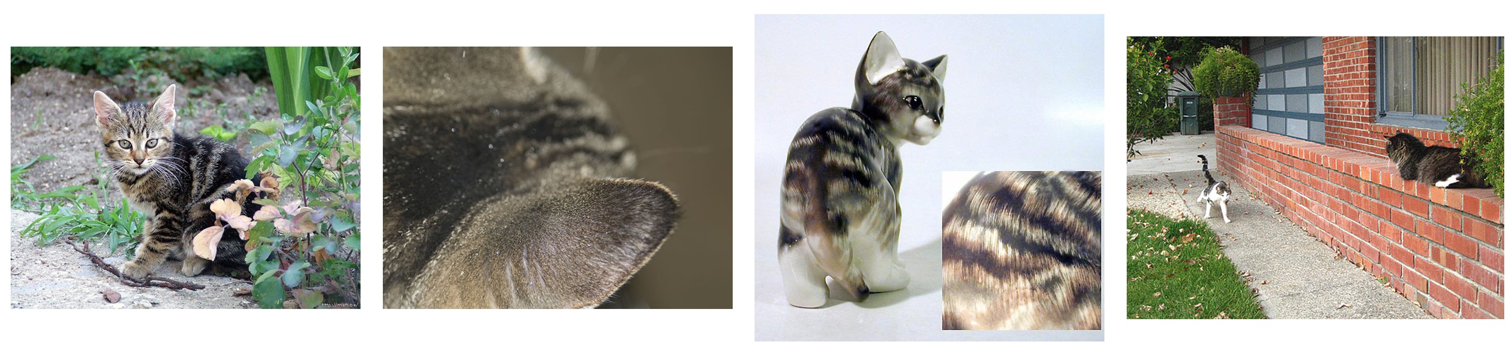
In popular visual datasets, the variance among images is high. The exactly same composite augmentation hence can lead to different latent deviation in the feature space. For instance, as illustrated in Fig. 2, target items of images may be of different size and shape, and may be located at different places. Therefore, naively enforcing all representations of augmented instances to have the same optimal deviation may not lead to the best performance.

To this end, Eq. 12 calculates the expectation of deviation in a minibatch first with each given length of augmentation composition. Eq. 12 hence aims to adjust the averaged latent deviations in a minibatch instead of every single one, which help better handle the variance.

Meanwhile, Eq. 12 replaces the computation of absolute value with $\text{softplus}(\cdot)$. As it has been demonstrated, the same augmentation may lead to different latent deviation, which means some augmented instances may still maintain all or almost all of their identity. $\text{softplus}(\cdot)$ has small gradient value with negative input, which avoids pushing apart representations which are supposed to be close to each other.

Figure 2: Images from a same category of a dataset. Target items may be of different sizes and colors, and may be located at different places in images. Thus same augmentation can have different effects on different images. ImageNet is used for illustration.

A.2 Derivation of $\theta_{d}$’s Update

We write the update of the encoder and PMNN as:

$$\begin{split}&\bm{\theta_{e}}^{\prime}=\bm{\theta_{e}}-\eta_{e}\nabla_{\bm{\theta_{e}}}\mathcal{L}_{u}(\bm{\theta_{e}},\bm{\theta_{d}})\\ &\bm{\theta_{d}}^{\prime}=\bm{\theta_{d}}-\eta_{d}\nabla_{\bm{\theta_{d}}}\text{CE}(\bm{x_{l}},y;\bm{\theta_{e}}(\bm{\theta_{d}}))\end{split}$$ (13)

With the overall loss function to optimize the encoder, the update of $\bm{\theta_{e}}$ with learning rate $\eta_{e}$ can be written as:

$$\begin{split}\bm{\theta_{e}}^{\prime}&=\bm{\theta_{e}}-\eta_{e}\cdot(\nabla_{\bm{\theta_{e}}}\mathcal{L}_{\text{contrast}}+\nabla_{\bm{\theta_{e}}}\mathcal{L}_{\text{consistent}})\end{split}$$ (14)

By applying chain rule, the update of $\bm{\theta_{d}}$ with learning rate $\eta_{d}$ can be rewritten as:

$$\begin{split}&\bm{\theta_{d}}^{\prime}=\bm{\theta_{d}}-\eta_{d}\cdot(\nabla_{\bm{\theta_{d}}}\text{CE}(\bm{x_{l}},y;\bm{\theta_{e}}(\bm{\theta_{d}})),\\ \mathrm{where}\quad&\ \nabla_{\bm{\theta_{d}}}\text{CE}(\bm{x_{l}},y;\bm{\theta_{e}}(\bm{\theta_{d}}))=\frac{\partial}{\partial\bm{\theta_{e}}}\text{CE}(\bm{x_{l}},y;\bm{\theta_{e}})\cdot\frac{\partial\bm{\theta_{e}}}{\partial\bm{\theta_{d}}}\end{split}$$ (15)

In Eq. 15, $\frac{\partial}{\partial\bm{\theta_{e}}}\text{CE}(\bm{x_{l}},y;\bm{\theta_{e}})$ is computable via back-propagation. Thus, we focus on the computation of $\frac{\partial\bm{\theta_{e}}}{\partial\bm{\theta_{d}}}$:

$$\begin{split}\frac{\partial\bm{\theta_{e}}}{\partial\bm{\theta_{d}}}&=\frac{\partial}{\partial\bm{\theta_{d}}}(\bm{\theta_{e}}^{\prime}-\eta_{e}\cdot(\nabla_{\bm{\theta_{e}}}\mathcal{L}_{\text{contrast}}+\nabla_{\bm{\theta_{e}}}\mathcal{L}_{\text{consistent}}))\\ &=-\eta_{e}\cdot\frac{\partial}{\partial\bm{\theta_{d}}}\frac{\partial}{\partial\bm{\theta_{e}}}\mathcal{L}_{\text{consistent}}\\ &=-\eta_{e}\cdot\frac{\partial}{\partial\bm{\theta_{d}}}\frac{\partial}{\partial\bm{\theta_{e}}}\mathrm{softplus}[\mathbb{E}_{i\in\mathcal{B}}[\mathrm{sim}(f_{\bm{\theta_{e}}}(\bm{x_{i}}^{\prime\prime}),f_{\bm{\theta_{e}}}(\bm{x_{i}}))-g_{\bm{\theta_{d}}}(\bm{V}(A))]]\end{split}$$ (16)

where $\bm{x_{i}}^{\prime\prime}$ denotes the augmented data, and $\bm{V}(A)$ denotes the composition vector of the corresponding augmentation.

To simplify the notation, we define:

$$\begin{split}k=&\mathbb{E}_{i\in\mathcal{B}}[\mathrm{sim}(f_{\theta_{e}}(\bm{x_{i}}^{\prime\prime}),f_{\bm{\theta_{e}}}(\bm{x_{i}}))-g_{\bm{\theta_{d}}}(\bm{V}(A)]\\ &simi=\mathbb{E}_{i\in\mathcal{B}}[\mathrm{sim}(f_{\bm{\theta_{e}}}(\bm{x_{i}}^{\prime\prime}),f_{\bm{\theta_{e}}}(\bm{x_{i}}))]\end{split}$$ (17)

Then from Eq. 16 and Eq. 17, we have:

$$\begin{split}\frac{\partial\bm{\theta_{e}}}{\partial\bm{\theta_{d}}}&=-\eta_{e}\cdot\frac{\partial}{\partial\bm{\theta_{d}}}(\frac{-e^{k}}{1+e^{k}}\cdot\frac{\partial}{\partial\bm{\theta_{e}}}simi)\\ &=-\eta_{e}\cdot\frac{e^{k}}{(1+e^{k})^{2}}\cdot\frac{\partial}{\partial\bm{\theta_{e}}}simi\cdot\frac{\partial}{\partial\bm{\theta_{d}}}\mathbb{E}_{i\in\mathcal{B}}[g_{\bm{\theta_{d}}}(\bm{V}(A))]\end{split}$$ (18)

We plug Eq. 18 in Eq. 15:

$$\begin{split}\nabla_{\bm{\theta_{d}}}CE(\bm{x_{l}},y;\bm{\theta_{e}})&=\frac{\partial}{\partial\bm{\theta_{e}}}CE(\bm{x_{l}},y;\bm{\theta_{e}})\cdot\\ &\ (-\eta_{e}\cdot\frac{e^{k}}{(1+e^{k})^{2}}\cdot\frac{\partial}{\partial\bm{\theta_{e}}}simi\cdot\frac{\partial}{\partial\bm{\theta_{d}}}\mathbb{E}_{i\in\mathcal{B}}[g_{\bm{\theta_{d}}}(\bm{V}(A))])\end{split}$$ (19)

In Equation 19, $\frac{\partial}{\partial\bm{\theta_{e}}}\text{CE}(\bm{x_{l}},y;\bm{\theta_{e}})$ can be approximated as follows:

$$\begin{split}\text{CE}(\bm{x_{l}},y;\bm{\theta_{e}}^{\prime})-\text{CE}(\bm{x_{l}},y;\bm{\theta_{e}})&=(\bm{\theta_{e}}^{\prime}-\bm{\theta_{e}})\cdot\frac{\partial}{\partial\bm{\theta_{e}}}\text{CE}(\bm{x_{l}},y;\bm{\theta_{e}})\\ \frac{\partial}{\partial\bm{\theta_{e}}}\text{CE}(\bm{x_{l}},y;\bm{\theta_{e}})&=\frac{CE(\bm{x_{l}},y;\bm{\theta_{e}}^{\prime})-\text{CE}(\bm{x_{l}},y;\bm{\theta_{e}})}{\bm{\theta_{e}}^{\prime}-\bm{\theta_{e}}}\\ &=\frac{\text{CE}(\bm{x_{l}},y;\bm{\theta_{e}}^{\prime})-\text{CE}(\bm{x_{l}},y;\bm{\theta_{e}})}{-\eta_{e}\cdot(\nabla_{\bm{\theta_{e}}}\mathcal{L}_{\text{contrast}}+\nabla_{\bm{\theta_{e}}}\mathcal{L}_{\text{consistent}})}\end{split}$$ (20)

Finally, PMNN’s update can be calculated as follows using back-propagation:

$$\begin{split}\nabla_{\bm{\theta_{d}}}\text{CE}(\bm{x_{l}},y;\bm{\theta_{e}})&=\frac{\text{CE}(\bm{x_{l}},y;\bm{\theta_{e}}^{\prime})-\text{CE}(\bm{x_{l}},y;\bm{\theta_{e}})}{-\eta_{e}\cdot(\nabla_{\bm{\theta_{e}}}\mathcal{L}_{\text{contrast}}+\nabla_{\bm{\theta_{e}}}\mathcal{L}_{\text{consistent}})}\cdot\\ &\qquad(-\eta_{e}\cdot\frac{e^{k}}{(1+e^{k})^{2}}\cdot\frac{\partial}{\partial\bm{\theta_{e}}}simi\cdot\frac{\partial}{\partial\bm{\theta_{d}}}\mathbb{E}_{i\in\mathcal{B}}[g_{\theta_{d}}(\bm{V}(A))])\\ &=\frac{e^{k}}{(1+e^{k})^{2}}\cdot(\text{CE}(\bm{x_{l}},y;\bm{\theta_{e}}^{\prime})-\text{CE}(\bm{x_{l}},y;\bm{\theta_{e}}))\cdot\\ &\qquad\frac{simi(\bm{\theta_{e}}^{\prime})-simi(\bm{\theta_{e}})}{\mathcal{L}_{u}(\bm{\theta_{e}}^{\prime})-\mathcal{L}_{u}(\bm{\theta_{e}})}\cdot\frac{\partial}{\partial\bm{\theta_{d}}}\mathbb{E}_{i\in\mathcal{B}}[g_{\theta_{d}}(\bm{V}(A))]\\ \mathrm{where}&\quad simi(\bm{\theta_{e}}^{\prime})=\mathbb{E}_{i\in\mathcal{B}}[\mathrm{sim}(f_{\theta_{e}^{\prime}}(x_{i}^{\prime\prime}),f_{\theta_{e}^{\prime}}(x_{i}))]\end{split}$$ (21)

References

- [1] Atilim Gunes Baydin, Robert Cornish, David Martinez Rubio, Mark Schmidt, and Frank Wood. Online learning rate adaptation with hypergradient descent. arXiv preprint arXiv:1703.04782, 2017.
- [2] Léon Bottou. Large-scale machine learning with stochastic gradient descent. In Proceedings of COMPSTAT’2010: 19th International Conference on Computational StatisticsParis France, August 22-27, 2010 Keynote, Invited and Contributed Papers, pages 177–186. Springer, 2010.
- [3] Yue Cao, Zhenda Xie, Bin Liu, Yutong Lin, Zheng Zhang, and Han Hu. Parametric instance classification for unsupervised visual feature learning. Advances in neural information processing systems, 33:15614–15624, 2020.
- [4] Mathilde Caron, Ishan Misra, Julien Mairal, Priya Goyal, Piotr Bojanowski, and Armand Joulin. Unsupervised learning of visual features by contrasting cluster assignments. Advances in neural information processing systems, 33:9912–9924, 2020.
- [5] Ting Chen, Simon Kornblith, Mohammad Norouzi, and Geoffrey Hinton. A simple framework for contrastive learning of visual representations. arXiv preprint arXiv:2002.05709, 2020.
- [6] Xinlei Chen, Haoqi Fan, Ross Girshick, and Kaiming He. Improved baselines with momentum contrastive learning. arXiv preprint arXiv:2003.04297, 2020.
- [7] Dan Ciregan, Ueli Meier, and Jürgen Schmidhuber. Multi-column deep neural networks for image classification. In 2012 IEEE conference on computer vision and pattern recognition, pages 3642–3649. IEEE, 2012.
- [8] Ekin D Cubuk, Barret Zoph, Dandelion Mane, Vijay Vasudevan, and Quoc V Le. Autoaugment: Learning augmentation strategies from data. In Proceedings of the IEEE/CVF conference on computer vision and pattern recognition, pages 113–123, 2019.
- [9] Ekin D Cubuk, Barret Zoph, Jonathon Shlens, and Quoc V Le. Randaugment: Practical automated data augmentation with a reduced search space. In Proceedings of the IEEE/CVF conference on computer vision and pattern recognition workshops, pages 702–703, 2020.
- [10] Mark Everingham, Luc Van Gool, Christopher KI Williams, John Winn, and Andrew Zisserman. The pascal visual object classes (voc) challenge. International journal of computer vision, 88:303–308, 2009.
- [11] Kaiming He, Haoqi Fan, Yuxin Wu, Saining Xie, and Ross Girshick. Momentum contrast for unsupervised visual representation learning. In Proceedings of the IEEE/CVF conference on computer vision and pattern recognition, pages 9729–9738, 2020.
- [12] Kaiming He, Xiangyu Zhang, Shaoqing Ren, and Jian Sun. Deep residual learning for image recognition. In Proceedings of the IEEE conference on computer vision and pattern recognition, pages 770–778, 2016.
- [13] Olivier Henaff. Data-efficient image recognition with contrastive predictive coding. In International conference on machine learning, pages 4182–4192. PMLR, 2020.
- [14] Qianjiang Hu, Xiao Wang, Wei Hu, and Guo-Jun Qi. Adco: Adversarial contrast for efficient learning of unsupervised representations from self-trained negative adversaries. In Proceedings of the IEEE/CVF Conference on Computer Vision and Pattern Recognition, pages 1074–1083, 2021.
- [15] Yannis Kalantidis, Mert Bulent Sariyildiz, Noe Pion, Philippe Weinzaepfel, and Diane Larlus. Hard negative mixing for contrastive learning. Advances in Neural Information Processing Systems, 33:21798–21809, 2020.
- [16] Alex Krizhevsky, Ilya Sutskever, and Geoffrey E Hinton. Imagenet classification with deep convolutional neural networks. Communications of the ACM, 60(6):84–90, 2017.
- [17] Junnan Li, Pan Zhou, Caiming Xiong, and Steven CH Hoi. Prototypical contrastive learning of unsupervised representations. arXiv preprint arXiv:2005.04966, 2020.
- [18] Tsung-Yi Lin, Michael Maire, Serge Belongie, James Hays, Pietro Perona, Deva Ramanan, Piotr Dollár, and C Lawrence Zitnick. Microsoft coco: Common objects in context. In Computer Vision–ECCV 2014: 13th European Conference, Zurich, Switzerland, September 6-12, 2014, Proceedings, Part V 13, pages 740–755. Springer, 2014.
- [19] Hanxiao Liu, Karen Simonyan, and Yiming Yang. Darts: Differentiable architecture search. arXiv preprint arXiv:1806.09055, 2018.
- [20] Ishan Misra and Laurens van der Maaten. Self-supervised learning of pretext-invariant representations. In Proceedings of the IEEE/CVF conference on computer vision and pattern recognition, pages 6707–6717, 2020.
- [21] Hieu Pham, Zihang Dai, Qizhe Xie, and Quoc V Le. Meta pseudo labels. In Proceedings of the IEEE/CVF conference on computer vision and pattern recognition, pages 11557–11568, 2021.
- [22] Ikuro Sato, Hiroki Nishimura, and Kensuke Yokoi. Apac: Augmented pattern classification with neural networks. arXiv preprint arXiv:1505.03229, 2015.
- [23] Patrice Y Simard, David Steinkraus, John C Platt, et al. Best practices for convolutional neural networks applied to visual document analysis. In Icdar. Edinburgh, 2003.
- [24] Yonglong Tian, Dilip Krishnan, and Phillip Isola. Contrastive multiview coding. In Computer Vision–ECCV 2020: 16th European Conference, Glasgow, UK, August 23–28, 2020, Proceedings, Part XI 16, pages 776–794. Springer, 2020.
- [25] Yonglong Tian, Chen Sun, Ben Poole, Dilip Krishnan, Cordelia Schmid, and Phillip Isola. What makes for good views for contrastive learning? Advances in neural information processing systems, 33:6827–6839, 2020.
- [26] Li Wan, Matthew Zeiler, Sixin Zhang, Yann Le Cun, and Rob Fergus. Regularization of neural networks using dropconnect. In International conference on machine learning, pages 1058–1066. PMLR, 2013.
- [27] Tongzhou Wang and Phillip Isola. Understanding contrastive representation learning through alignment and uniformity on the hypersphere. In International Conference on Machine Learning, pages 9929–9939. PMLR, 2020.
- [28] Xiao Wang and Guo-Jun Qi. Contrastive learning with stronger augmentations. arXiv preprint arXiv:2104.07713, 2021.
- [29] Zhirong Wu, Yuanjun Xiong, Stella X Yu, and Dahua Lin. Unsupervised feature learning via non-parametric instance discrimination. In Proceedings of the IEEE conference on computer vision and pattern recognition, pages 3733–3742, 2018.
- [30] Yuning You, Tianlong Chen, Yang Shen, and Zhangyang Wang. Graph contrastive learning automated. In International Conference on Machine Learning, pages 12121–12132. PMLR, 2021.