Analysis of view aliasing for the generalized Radon transform in $\mathbb{R}^{2}$

Abstract.

In this paper we consider the generalized Radon transform $\mathcal{R}$ in the plane. Let $f$ be a piecewise smooth function, which has a jump across a smooth curve $\mathcal{S}$. We obtain a formula, which accurately describes view aliasing artifacts away from $\mathcal{S}$ when $f$ is reconstructed from the data $\mathcal{R}f$ discretized in the view direction. The formula is asymptotic, it is established in the limit as the sampling rate $\epsilon\to 0$. The proposed approach does not require that $f$ be band-limited. Numerical experiments with the classical Radon transform and generalized Radon transform (which integrates over circles) demonstrate the accuracy of the formula.

1. Introduction

Resolution of image reconstruction from discrete data is one of the fundamental questions in imaging. The most direct approach to estimating resolution utilizes the notions of the point spread function (PSF) and modulation transfer function (MTF) [1, Sections 12.2, 12.3]. This and other similar approaches allow rigorous theoretical analysis of only the simplest settings, such as inversion of the classical Radon transform. For the most part, resolution of reconstruction in more difficult settings (e.g., inversion of the cone beam transform) is analyzed by heuristic arguments, numerically, or via measurements [2, 3, 4].

Sampling theory provides a related approach to investigating resolution [5, 6, 7, 8, 9, 10, 11, 12, 13, 14]. Consider, for example, the classical Radon transform in $\mathbb{R}^{2}$

(1.1) $$\hat{f}(\alpha,p)=\int_{\mathbb{R}^{2}}f(x)\delta(\vec{\alpha}\cdot x-p)\text{d}x,\ \vec{\alpha}=(\cos\alpha,\sin\alpha).$$

The corresponding discrete data are

(1.2) $$\hat{f}(\alpha_{k},p_{j}),\ \alpha_{k}=\bar{\alpha}+k\Delta\alpha,\ p_{j}=\bar{p}+j\Delta p,\ \alpha_{k}\in[0,2\pi),j\in\mathbb{Z},$$

for some fixed $\bar{\alpha}$, $\bar{p}$ and $\Delta\alpha$, $\Delta p$. Assume that $f$ is essentially band-limited (in the classical sense). This means that, with high accuracy, its Fourier transform $\tilde{f}(\xi)$ is supported in some ball $|\xi|\leq B$. The sampling theory predicts the rates $\Delta\alpha$, $\Delta p$ with which $\hat{f}(\alpha,p)$ should be sampled, so that reconstruction of $f$ from discrete data does not contain aliasing artifacts. Since the essential band-limit $B$ is related to the size of the smallest detail in $f$, a typical prescription of the theory can be loosely formulated as follows: given the size of the smallest detail in $f$, the minimal sampling rates to avoid aliasing are $\Delta\alpha$, $\Delta p$. Alternatively, the theory determines the size of the smallest detail in $f$ that can be resolved given the rates $\Delta\alpha$, $\Delta p$.

A microlocal approach to sampling was developed recently [15, 16, 17]. In this approach $f$ is assumed to be band-limited in the semiclassical sense (i.e., the semiclassical wavefront set $\text{WF}_{h}(f)$ is compact). Alternatively, the assumption is that the data represent discrete values of the convolution $w*\mathcal{R}f$. Here $\mathcal{R}$ is the generalized Radon transform, and $w$ is a semiclassically bandlimited mollifier. The mollifier models the detector aperture function. The goal is to accurately recover the semiclassical singularities of $f$ and avoid aliasing. If the sampling requirement is violated, the theory predicts the location and frequency of aliasing artifacts.

In [18, 19, 20, 21, 22], the author developed an alternative analysis of resolution (we call it Local Resolution Analysis, or LRA). The main results in these papers are simple expressions describing the reconstruction from discrete values of $\mathcal{R}f$ or $w*\mathcal{R}f$ in a neighborhood of the singularities of $f$ in a variety of settings. We call these expressions the Discrete Transition Behavior (DTB). The DTB provides a direct, quantitative link between the sampling rate and resolution. In these papers such a link is established for a wide range of integral transforms, conormal distributions $f$, and reconstruction operators. In [23, 24] LRA was generalized to objects with rough boundaries in $\mathbb{R}^{2}$. Neither $f$ nor the mollifier $w$ (if applied) is required to be bandlimited.

Suppose $\Delta p=\epsilon$ and $\Delta\alpha=\kappa\epsilon$, where $\kappa>0$ is fixed. The DTB is an accurate approximation of the reconstruction in an $\epsilon$-neighborhood of the singular support of $f$ in the limit as $\epsilon\to 0$. Therefore, the DTB provides much more than a single measure of resolution (e.g., the size of the smallest detail that can be resolved). Given the DTB function, the user may decide in a fully quantitative way what sampling rate is required to achieve a user-defined reconstruction quality. The notion of quality may include resolution (which can be described in any desired way) and/or any other requirement the user desires. Thus, the LRA answers precisely the question of the required sampling rate to guarantee the required resolution (understood broadly).

The only item missing from the LRA until now was analysis of aliasing. Some earlier results on the analysis of aliasing artifacts (more precisely, view aliasing artifacts) are in [25] and [1, Section 12.3.2]. They include an approximate formula for the artifacts far from a small, radially symmetric object. More recent results are in [15, 16, 17]. These include the prediction of the location and frequency of the artifacts, qualitative analysis of the artifacts generated by various edges (e.g., flat, convex, and a corner), as well as their numerical illustrations.

In this paper we generalize the LRA to the analysis of view aliasing. We call it the Localized Aliasing Analysis, or LAA. Our main result is Theorem 2.5, where a precise, quantitative formula describing aliasing artifacts is stated. The formula is asymptotic, it is established in the limit as the sampling rate $\epsilon\to 0$ (which is the same assumption as in [15, 16, 17]). Similarly to the LRA, the LAA is very flexible. In this paper we consider the generalized Radon transform in $\mathbb{R}^{2}$ and apply it to functions with jump discontinuities across smooth curves. Similarly to [18, 19, 20, 21, 22], we believe that the LAA is generalizable, and that it is capable of predicting aliasing artifacts for a wide range of integral transforms, conormal distributions $f$, and reconstruction operators.

To avoid confusion, we clarify the meaning of the terms “resolution” and “aliasing” used in this paper. For simplicity, we will use the example of a jump discontinuity across a smooth curve $\mathcal{S}$. Resolution at $x_{0}\in\mathcal{S}$ means the extent to which the boundary at the jump (i.e., $\mathcal{S}$) is blurred when the image is reconstructed in a neighborhood of $x_{0}$ from discrete data. This blurring is accurately described by the DTB function mentioned above. The derivation of the DTB function accounts for possible artifacts that may arise due to aliasing from the parts of $\mathcal{S}$ in a neighborhood of $x_{0}$. In other words, LRA treats local aliasing as part of resolution analysis. In this paper, the term “aliasing” stands for rapidly oscillating artifacts away from $\mathcal{S}$ that are caused by aliasing from $\mathcal{S}$.

The paper is organized as follows. In section 2 we describe the set-up, formulate the assumptions, and state the main result – Theorem 2.5. This theorem provides a simple formula that describes aliasing artifacts. We also discuss various quantities used in the formula, and state a corollary that describes what the formula looks like in the case of the classical Radon transform. The proof of Theorem 2.5 is in section 3. Section 4.1 establishes a few useful properties of the function $\Psi$, in terms of which the artifacts are described. An algorithm for computing $\Psi$ numerically is in Section 4.2. Section 5 contains numerical experiments with the classical and generalized Radon transforms. The latter integrates over circles. Details of implementation, which illustrate the use of the theorem, are provided. All experiments demonstrate a good match between reconstruction and prediction. Proofs of some lemmas are in appendix A.

2. Preliminaries

2.1. Generalized Radon transform

Let $p=\mathcal{P}_{*}(\alpha,x)$ be a defining function for the generalized Radon transform $\mathcal{R}$:

(2.1) $$\hat{f}(\alpha,p)=\int_{\mathcal{S}_{\alpha,p}}W(\alpha,p;x)f(x)\text{d}A,\ \mathcal{S}_{\alpha,p}:=\{x\in\mathbb{R}^{2}:\mathcal{P}_{*}(\alpha,x)=p\},\alpha\in\Omega,p\in\mathbb{R},$$

where $W\in C^{\infty}(\Omega\times\mathbb{R}\times U)$ is some (known) integration weight, $\text{d}A$ is the length element on the curve $\mathcal{S}_{\alpha,p}$, $U\subset\mathbb{R}^{2}$ is a small open set, and $\Omega\subset\mathbb{R}$ is a small interval. Similarly to the classical Radon transform, we think about $\alpha$ as the polar angle, and $p$ - as the affine variable. However, since we consider the generalized Radon transform, these variables admit many alternative interpretations. See [26, 27] for more information and references about generalized Radon transforms, their properties and applications.

Let $\mathcal{S}$ be a $C^{\infty}$ curve. Let $(\alpha_{\star},p_{\star})$ be a pair such that $\mathcal{S}_{\alpha_{\star},p_{\star}}$ is tangent to $\mathcal{S}$ at some $y_{0}\in\mathcal{S}{\color[rgb]{0,0,0}\cap U}$. To simplify notation, denote $\mathcal{S}_{\star}:=\mathcal{S}_{\alpha_{\star},p_{\star}}$. We will compute a reconstruction in a small neighborhood of some point $x_{0}\not\in\mathcal{S}_{\star}$. Let $H(y)=0$ be an equation for $\mathcal{S}$ in a neighborhood of $y_{0}$. The function $H$ is smooth, and $\text{d}H(y)\not=0$, $y\in\mathcal{S}$. Multiplying $H$ by a constant if necessary, we can assume that $\mathcal{P}_{*}$ satisfies the equations

(2.2) $$\mathcal{P}_{*}(\alpha_{\star},x_{0})=\mathcal{P}_{*}(\alpha_{\star},y_{0})=p_{\star},\ \text{d}_{x}\mathcal{P}_{*}(\alpha_{\star},y_{0})=\text{d}H(y_{0}).$$

Assumptions 2.1 (Properties of $\mathcal{P}_{*}$).

         

1. $\mathcal{P}_{*}\in C^{\infty}(\Omega\times{\color[rgb]{0,0,0}U})$, and $\text{d}_{x}\mathcal{P}_{*}(\alpha,x)\not=0$, $x=x_{0},y_{0}$;

2. Equations (2.2) hold;

3. $\partial_{\alpha}\mathcal{P}_{*}(\alpha_{\star},x_{0})\not=\partial_{\alpha}\mathcal{P}_{*}(\alpha_{\star},y_{0})$ (the Bolker condition);

4. One has

   (2.3) $$M:=(\vec{\Theta}_{0}^{\perp}\cdot\partial_{y})^{2}(\mathcal{P}_{*}(\alpha_{\star},y)-H(y))|_{y=y_{0}}>0,$$

   where $\vec{\Theta}_{0}^{\perp}$ is a unit vector orthogonal to $\text{d}H(y_{0})$; and

5. There exists $c>0$ such that $y_{0}\not\in\mathcal{S}_{\alpha,p}$ for any $\alpha\in\Omega$ and $|p-p_{\star}|\geq c$.

Assumption 2.1(4) is equivalent to the condition that the curvatures of $\mathcal{S}$ and $\mathcal{S}_{\star}$ at $y_{0}$ are not equal. In other words, the order of contact between $\mathcal{S}$ and $\mathcal{S}_{\star}$ is one (and not higher). For example, if one of the two curves is flat at $y_{0}$, then $M\not=0$ as long as the other one is not flat. The requirement that $M$ be positive is not restrictive. If $M<0$, we can flip the $p$-axis and replace $H\to-H$, $\mathcal{P}_{*}\to-\mathcal{P}_{*}$ to make $M$ positive. The essential requirement is that $M\not=0$.

The requirement $M>0$ means that $\mathcal{S}_{\alpha_{\star},p_{\star}+\delta}$ intersects $\mathcal{S}$ at two points near $y_{0}$ when $\delta>0$, and does not intersect $\mathcal{S}$ near $y_{0}$ – if $\delta<0$ (see Figure 1). In what follows we set

(2.4) $$\vec{\Theta}_{0}:=\pm\text{d}H(y_{0}),$$

and the sign ($+$ or $-$) is selected so that $\vec{\Theta}_{0}$ points towards the part of $\mathcal{S}_{\alpha_{\star},p_{\star}+\delta}$, $0<\delta\ll 1$, located between its two intersection points with $\mathcal{S}$ (see Figure 1).

Shrinking, if necessary, $\Omega$ and $U$ further, we may assume that there is no other pair $(\alpha’,p’)\not=(\alpha_{\star},p_{\star})$, $\alpha’\in\Omega$, such that $x_{0}\in\mathcal{S}_{\alpha’,p’}$, and $\mathcal{S}_{\alpha’,p’}$ is tangent to $\mathcal{S}$ at $y_{0}$.

Figure 1. Illustration of the curves $\mathcal{S}$ and $\mathcal{S}_{\alpha,p}$.

Let $\mathcal{P}(\alpha)$, $\alpha\in\Omega$, be the function defined by the requirement that the curves $\mathcal{S}_{\alpha,\mathcal{P}(\alpha)}$ be tangent to $\mathcal{S}$ in a neighborhood of $y_{0}$. Figure 2 illustrates the function $\mathcal{P}(\alpha)$ in the case of the classical Radon transform (left panel) and the generalized Radon transform that integrates over circles (right panel). The circles have arbitrary radii and centers on a given curve $z(\alpha)\in\Gamma$, $\alpha\in\Omega$. Consider the latter case. Suppose, for example, that $\mathcal{S}$ is a circle with radius $r$ and center $a$. Then, globally, there are two such functions: $\mathcal{P}(\alpha)=|z(\alpha)-a|\pm r$. See also Section 5.2 for more details about the circular Radon transform.

The following simple lemma is proven in appendix A.1.

Figure 2. Illustration of the function $\mathcal{P}(\alpha)$. Left panel - the classical Radon transform that integrates over lines. Right panel - the generalized Radon transform that integrates over circles with centers on a given curve parametrized by $\alpha$ (denoted $\Gamma$ in the figure).

Lemma 2.2.

For a sufficiently small neighborhood $\Omega\ni\alpha_{\star}$, one has

(2.5) $$\mathcal{P}(\alpha_{\star})=p_{\star},\ \mathcal{P}(\alpha)\in C^{\infty}(\Omega),\ {\color[rgb]{0,0,0}\partial_{\alpha}\mathcal{P}_{*}(\alpha_{\star},y_{0})=\mathcal{P}’(\alpha_{\star}).}$$

From assumptions 2.1(1, 3) and Lemma 2.2,

(2.6) $$u_{0}:=\text{d}_{x}\mathcal{P}_{*}(\alpha_{\star},x_{0})\not=0,\ \mu_{0}:=\partial_{\alpha}(\mathcal{P}_{*}(\alpha_{\star},x_{0})-\mathcal{P}(\alpha_{\star}))\not=0.$$

2.2. Remaining assumptions and main result

Consider a function $f(x)$ on the plane, $x\in\mathbb{R}^{2}$. We suppose that

Assumptions 2.3 (Properties of $f$).

         

1. $\text{supp}(f)\subset U$, and $\text{diam}(U)$ is sufficiently small;

2. There exist open sets $D_{\pm}$ and functions $f_{\pm}\in C^{\infty}(\mathbb{R}^{2})$ such that

   (2.7) $$\begin{split}&f(x)\equiv f_{-}(x),\ x\in D_{-},\ f(x)\equiv f_{+}(x),\ x\in D_{+},\\ &D_{-}\cap D_{+}=\varnothing,\ D_{-}\cup D_{+}=U\setminus\mathcal{S};\end{split}$$

   and

3. $\mathcal{S}\cap U$ is a $C^{\infty}$ curve.

Thus, $\text{sing\,supp}(f)\subset\mathcal{S}$. In general, $f_{-}(x)\not=f_{+}(x)$, $x\in\mathcal{S}$, so $f$ may have a jump across $\mathcal{S}$. Note that whether $x_{0}\in U$ or not is irrelevant. Also, when $U$ shrinks towards $y_{0}$, $\mathcal{S}$ does not change. Thus, $\mathcal{S}\cap U$ is a small segment of $\mathcal{S}$ around $y_{0}$. With this understanding, in what follows we do not distinguish between $\mathcal{S}$ and $\mathcal{S}\cap U$.

Similarly to [17], we consider semi-discrete data

(2.8) $$\hat{f}_{\epsilon}(\alpha_{k},p):=\int w_{\epsilon}(p-s)\hat{f}(\alpha_{k},s)\text{d}s,\ \alpha_{k}:=k\Delta\alpha,\ p\in\mathbb{R},\ w_{\epsilon}(t):=\epsilon^{-1}w(t/\epsilon),$$

where $w$ is a mollifier (e.g., the detector aperture function), $\Delta\alpha=\kappa\epsilon$, and $\kappa>0$ is fixed. It is reasonable to assume that the support of $w_{\epsilon}$ is of size $O(\epsilon)$, because sampling rates along $\alpha$ and $p$ are usually of the same order of magnitude.

Assumptions 2.4 (Assumptions about the mollifier $w$).

         

1. $w$ is compactly supported and $w’\in L^{q}(\mathbb{R})$ for some $q>2$; and

2. $\int w(p)\text{d}p=1$.

Hence, the data (2.8) represent the integrals of $f$ along thin strips around $\mathcal{S}_{\alpha_{k},p}$, and their width ($=O(\epsilon)$) is determined by $\epsilon$ and the support of $w$. In the ideal case (not considered in this paper) , where $w$ is the Dirac $\delta$-function, the data represent the integrals of $f$ along $\mathcal{S}_{\alpha_{k},p}$.

Reconstruction from the data (2.8) is achieved by the formula

(2.9) $$f_{\epsilon}^{\text{rec}}(x)=-\frac{\Delta\alpha}{2\pi}\sum_{\alpha_{k}\in\Omega}\frac{\omega(\alpha_{k},x)}{\pi}\int\frac{\partial_{p}\hat{f}_{\epsilon}(\alpha_{k},p)}{p-\mathcal{P}_{*}(\alpha_{k},x)}\text{d}p,\ x\in U’,$$

where $U’$ is a small neighborhood of $x_{0}$, and $\omega\in C^{\infty}(\Omega\times U’)$ is some weight function. This is a discretized (in $\alpha$) version of the classical FBP inversion formula [28] adapted to the generalized Radon transform in $\mathbb{R}^{2}$ (e.g., as it was done in [29, 30]). The integral with respect to $p$, which is understood in the principal value sense, is the filtering step (the Hilbert transform). The exterior sum is a quadrature rule corresponding to the backprojection integral.

To better understand (2.9), we consider its continuous analogue. Suppose $w$ is the $\delta$-function. The continuous version of (2.9) reads

(2.10) $$f^{\text{rec}}=\mathcal{R}^{*}(\mathcal{H}\partial_{p})\mathcal{R}f.$$

Here $\mathcal{R}^{*}$ is a weighted adjoint transform, and $\mathcal{H}$ is the Hilbert transform acting with respect to $p$. By imposing additional restrictions on $\mathcal{P}_{*}$, $\omega$, and $W$ we can ensure that $\mathcal{R}^{*}(\mathcal{H}\partial_{p})\mathcal{R}$ is a $\Psi$DO of order zero (see e.g. [31, 29]) with some other desired properties (e.g., elliptic, principal symbol equal 1). We do not do this, since our focus here is only the reconstruction of rapidly oscillating artifacts in $f_{\epsilon}^{\text{rec}}$ away from $\mathcal{S}$. In particular, no attempt is made to achieve exact reconstruction. In view of this we impose only a minimal set of conditions that guarantee that Theorem 2.5 holds. These conditions do not guarantee that $\mathcal{R}^{*}(\mathcal{H}\partial_{p})\mathcal{R}$ is a $\Psi$DO.

Introduce the following functions:

(2.11) $$\begin{split}\psi(\hat{q}):=&(1/2)\int_{0}^{\infty}w(\hat{q}+\hat{p})\hat{p}^{-1/2}\text{d}\hat{p},\ {\color[rgb]{0,0,0}\hat{q}\in\mathbb{R},}\\ \Psi(h;a,r):=&\sum_{{\color[rgb]{0,0,0}k\in\mathbb{Z}}}\left[\psi\left(a(k-r)+h\right)-\psi\left(a(k-r)\right)\right],\ \color[rgb]{0,0,0}h,a,r\in\mathbb{R},a\not=0,\\ \color[rgb]{0,0,0}\Psi(h;0,r):=&{\color[rgb]{0,0,0}0,\ h,r\in\mathbb{R}},\end{split}$$

and

(2.12) $$\begin{split}\Delta f(y_{0})=&\lim_{\epsilon\to 0^{+}}(f(y_{0}+\epsilon\vec{\Theta}_{0})-f(y_{0}-\epsilon\vec{\Theta}_{0})).\end{split}$$

Various properties of $\psi$ and $\Psi$ (e.g., that $\psi$ is continuous and decays sufficiently fast, so that the series in the definition of $\Psi$ is absolutely convergent) are established in Sections 3.1 and 4. Our main result is as follows.

Theorem 2.5.

Suppose $W\in C^{\infty}(\Omega\times\mathbb{R}\times U)$, and $\omega\in C^{\infty}(\Omega\times U’)$ for some small open sets $\Omega\ni\alpha_{\star}$, $U\ni y_{0}$, and $U’\ni x_{0}$. Under the assumptions 2.1, 2.3, and 2.4, one has

(2.13) $$\begin{split}\epsilon^{-1/2}&(f_{\epsilon}^{\text{rec}}(x_{0}+\epsilon\check{x})-f_{\epsilon}^{\text{rec}}(x_{0}))=c\Psi(u_{0}\cdot\check{x};\kappa\mu_{0},k_{\star})+O(\epsilon^{1/2}),\ \epsilon\to 0,\\ c:=&-\frac{\kappa\omega(\alpha_{\star},x_{0})W(\alpha_{\star},p_{\star};y_{0})}{\pi}(2/M)^{1/2}\,\Delta f(y_{0}),\\ \color[rgb]{0,0,0}k_{\star}:=&\color[rgb]{0,0,0}\alpha_{\star}/\Delta\alpha,\ \kappa:=\Delta\alpha/\epsilon,\color[rgb]{0,0,0}\end{split}$$

where $M$ is defined in (2.3), $u_{0}$ and $\mu_{0}$ are defined (2.6), and the $O(\epsilon^{1/2})$ term is uniform with respect to $\check{x}$ confined to any bounded set.

To help the reader, we discuss various quantities occurring in (2.13).

1. $\check{x}$ is a rescaled displacement from a fixed point $x_{0}$ to a nearby reconstruction point $x$: $\check{x}=(x-x_{0})/\epsilon$;

2. For the classical Radon transform (CRT), $\mathcal{P}_{*}(\alpha,x)=\vec{\alpha}\cdot x$, where $\alpha$ and $\vec{\alpha}$ are related by $\vec{\alpha}=(\cos\alpha,\sin\alpha)$;

3. $\alpha_{\star},p_{\star}$ are the values such that the integration curve $\mathcal{S}_{\star}=\mathcal{S}_{\alpha_{\star},p_{\star}}$ contains $x_{0}$ is tangent to $\mathcal{S}$ at some point, denoted $y_{0}$ (see Figure 1);

4. $W(\alpha,p;y)$ and $\omega(\alpha,x)$ are integration weights in $\mathcal{R}$ and its adjoint (see (2.1), (2.9), (2.10), and the discussion around the latter equation). For the CRT, $W(\alpha,p;y)\equiv 1$ and $\omega(\alpha,x)\equiv 1$;

5. $\kappa=\Delta\alpha/\epsilon$, where $\Delta\alpha$ is the step-size along $\alpha$;

6. Up to a nonzero factor, $M$ is the difference of curvatures of $\mathcal{S}$ and $\mathcal{S}_{\star}$ at $y_{0}$;

7. $\Delta f(y_{0})$ is the value of the jump of $f$ across $\mathcal{S}$ at $y_{0}$;

8. $k_{\star}=\alpha_{\star}/\Delta\alpha$ is the “index” value corresponding to the angle $\alpha_{\star}$. We put the word index in quotes, because $k_{\star}$ is not necessarily an integer. As is easily seen from (2.11) and (2.13), only the fractional part of $k_{\star}$ is important;

9. The quantities $u_{0}:=\text{d}_{x}\mathcal{P}_{*}(\alpha_{\star},x_{0})$ and $\mu_{0}:=\partial_{\alpha}(\mathcal{P}_{*}(\alpha_{\star},x_{0})-\mathcal{P}(\alpha_{\star}))$ depend on the properties of the Radon transform (via the function $\mathcal{P}_{*}$) and the curve $\mathcal{S}$. For the CRT, $u_{0}=\vec{\alpha}_{\star}$ and $\mu_{0}=\vec{\alpha}_{\star}^{\perp}\cdot(x_{0}-y_{0})$, so $|\mu_{0}|=|x_{0}-y_{0}|$.

The following corollary, which follows immediately from Theorem 2.5, illustrates what eq. (2.13) looks like in the case of the classical Radon transform.

Corollary 2.6.

Let $\mathcal{R}$ be the classical Radon transform. Under the assumptions of Theorem 2.5 one has

(2.14) $$\begin{split}\epsilon^{-1/2}&(f_{\epsilon}^{\text{rec}}(x_{0}+\epsilon\check{x})-f_{\epsilon}^{\text{rec}}(x_{0}))=c\Psi(\alpha_{\star}\cdot\check{x};\kappa\vec{\alpha}_{\star}^{\perp}\cdot(x_{0}-y_{0}),k_{\star})+O(\epsilon^{1/2}),\ \epsilon\to 0,\\ c:=&-(\kappa/\pi)(2r)^{1/2}\,\Delta f(y_{0}),\ k_{\star}:=\alpha_{\star}/\Delta\alpha,\ \kappa:=\Delta\alpha/\epsilon,\end{split}$$

where $r$ is the radius of curvature of $\mathcal{S}$ at $y_{0}$, and the $O(\epsilon^{1/2})$ term is uniform with respect to $\check{x}$ confined to any bounded set.

See Section 5 for more details on how to apply (2.13) for the classical and circular Radon transforms.

3. Proof of Theorem 2.5

By (2.6), $u_{0}\not=0$, $\mu_{0}\not=0$. By linearity of the Radon transform, we can assume that the support of $f$ is contained in a small neighborhood of $y_{0}$ (i.e., by shrinking $U$ as much as necessary). By assumption 2.1(5), shrinking $U$ and $\Omega$ even more, we can assume that there exists $c>0$ such that

(3.1) $$\begin{split}&\mathcal{S}_{\alpha,p}\cap U=\varnothing\text{ for any }\alpha\in\Omega,|p-p_{\star}|\geq c.\end{split}$$

Then

(3.2) $$\hat{f}(\alpha,p)=\varphi_{1}(\alpha)(p-\mathcal{P}(\alpha))_{+}^{1/2}+\varphi_{2}(\alpha,p)(p-\mathcal{P}(\alpha))_{+}^{3/2}+\varphi_{3}(\alpha,p),\ \alpha\in\Omega,p\in\mathbb{R},$$

where $\varphi_{1}\in C_{0}^{\infty}(\Omega)$, $\varphi_{2,3}\in C^{\infty}(\Omega\times\mathbb{R})$, and

(3.3) $$\varphi_{1}(\alpha_{\star})=W(\alpha_{\star},p_{\star};y_{0})\Delta f(y_{0})2(2/M)^{1/2}.$$

For the classical Radon transform this result is established in [32, 33]. For the generalized Radon transform it easily follows from $\text{d}_{x}\mathcal{P}_{*}(\alpha_{\star},y_{0})\not=0$ and $M\not=0$ (see assumptions 2.1(1, 4)) by applying the method of proof of Lemma 3.5 in [21].

Since $f(x)$ is compactly supported, $\hat{f}(\alpha,p)$ is compactly supported in $p$ by (3.1). Hence we can assume that $\varphi_{2}(\alpha,p)$ is compactly supported as well, and

(3.4) $$\varphi_{3}(\alpha,p)\equiv-\varphi_{1}(\alpha)(p-\mathcal{P}(\alpha))_{+}^{1/2},\ \alpha\in\Omega,|p|\geq c,$$

for some $c$.

The idea of the proof is to split $\hat{f}$ into three terms using (3.2), substitute each of them one by one into (2.8), (2.9), and investigate the resulting expressions separately.

3.1. Beginning of proof. Estimate of the leading term.

Replace $\hat{f}(\alpha,s)$ with $\varphi_{1}(\alpha)(s-\mathcal{P}(\alpha))_{+}^{1/2}$ in (2.8) and substitute into (2.9). After simple transformations we get

(3.5) $$\begin{split}f_{\epsilon}^{\text{rec-1}}(x):=&-\frac{\Delta\alpha}{2\pi\epsilon^{1/2}}\sum_{\alpha_{k}\in\Omega}\omega(\alpha_{k},x)\varphi_{1}(\alpha_{k})\psi((\mathcal{P}_{*}(\alpha_{k},x)-\mathcal{P}(\alpha_{k}))/\epsilon),\\ \psi(\hat{q}):=&(2\pi)^{-1}\int(\hat{p}-\hat{q})^{-1}\int w(\hat{p}-\hat{s})\hat{s}_{+}^{-1/2}\text{d}\hat{s}\text{d}\hat{p}.\end{split}$$

After additional transformations with the help of the integral (3.13), $\psi$ simplifies to the expression in (2.11). These transformations are justified by applying $\psi$ in (3.5) to a test function and changing the order of integration using the result in [34, Section III.28.4]. In turn, (2.11) gives

(3.6) $$\begin{split}&\psi(\hat{q})=0,\ \hat{q}>c;\quad{\color[rgb]{0,0,0}\psi(\hat{q})\ \text{ is uniformly continuous on $\mathbb{R}$};}\\ &\psi^{(n)}(\hat{q})=c_{n}(-\hat{q})^{-(1/2)-n}+O(|\hat{q}|^{-(3/2)-n}),\ \hat{q}<-c,\hat{q}\to-\infty,n=0,1,2,\dots,\\ \end{split}$$

for some $c>0$ and $c_{n}$. Since $\hat{p}_{+}^{-1/2}\in L_{loc}^{q’}(\mathbb{R})$ for any $q’<2$, Assumption 2.4(1) and [35, Exercise 11, p. 196] imply that $\psi$ is uniformly continuous on $\mathbb{R}$. Note that $\psi(\hat{q})$ is of limited smoothness on a compact set, outside of which $\psi$ is $C^{\infty}$.

Using the notation in (2.6) and (2.11) we formulate the following result

Lemma 3.1.

Under the assumptions of Theorem 2.5 one has

(3.7) $$\begin{split}\epsilon^{-1/2}(f_{\epsilon}^{\text{rec-1}}(x_{0}+\epsilon\check{x})-&f_{\epsilon}^{\text{rec-1}}(x_{0}))\\ =&-\frac{\kappa\omega(\alpha_{\star},x_{0})\varphi_{1}(\alpha_{\star})}{2\pi}\Psi(u_{0}\cdot\check{x};\mu_{0}\kappa,k_{\star})+O(\epsilon^{1/2}),\end{split}$$

where the $O(\epsilon^{1/2})$ term is uniform with respect to $\check{x}$ confined to any bounded set.

The proof of the lemma is in subsection A.2.

3.2. The second term

Similarly, replace $\hat{f}(\alpha,s)$ with $\varphi_{2}(\alpha,s)(s-\mathcal{P}(\alpha))_{+}^{3/2}$ in (2.8) and substitute into (2.9). After simple transformations we get with some $c$

(3.8) $$\begin{split}f_{\epsilon}^{\text{rec-2}}(x):=&c\epsilon\sum_{\alpha_{k}\in\Omega}\omega(\alpha_{k},x)g_{2}(\mathcal{P}_{*}(\alpha_{k},x),\mathcal{P}(\alpha_{k}),\alpha_{k}),\ x=x_{0}+\epsilon\check{x},\\ g_{2}(p,q,\alpha):=&\int(t-p)^{-1}\partial_{t}\int w_{\epsilon}(t-s)\varphi_{2}(\alpha,s)(s-q)_{+}^{3/2}\text{d}s\text{d}t,\\ &{\color[rgb]{0,0,0}p=\mathcal{P}_{*}(\alpha_{k},x),\ q=\mathcal{P}(\alpha_{k}).}\end{split}$$

Therefore, in (3.8) $p,q$ satisfy

(3.9) $$\begin{split}|p|\leq\sup_{\alpha\in\Omega}|\mathcal{P}_{*}(\alpha,x_{0})|+O(\epsilon),\ |q|\leq c,\end{split}$$

where $c$ is the same as in (3.1). Reducing, if necessary, $\Omega$ further, we can assume that the supremum in (3.9) is bounded. Thus, $|p|,|q|\leq P$ for some $P<\infty$. For simplicity, the dependence of $g_{2}$, $\varphi_{2}$, and related functions on $\alpha$ will be omitted from notation. Rewrite $g_{2}$ as follows:

(3.10) $$g_{2}(p,q)=\int w_{\epsilon}(p-t)\int(s-t)^{-1}\partial_{s}\left(\varphi_{2}(s)(s-q)_{+}^{3/2}\right)\text{d}s\text{d}t.$$

Using the results in [36, §8.3], we find

(3.11) $$\begin{split}g_{2}(p,q)&=\int w_{\epsilon}(p-t)\left(\varphi_{2,1}(t,q)(t-q)_{-}^{1/2}+\varphi_{2,2}(t,q)\right)\text{d}t\end{split}$$

for some smooth and bounded $\varphi_{2,1}$ and $\varphi_{2,2}$. The same result can be obtained by elementary means by writing

(3.12) $$\int_{0}^{\infty}\frac{\varphi(s)}{s^{1/2}(s-\rho)}\text{d}s=\varphi(\rho)\int_{0}^{\infty}\frac{\text{d}s}{s^{1/2}(s-\rho)}+\int_{0}^{\infty}\frac{\varphi(s)-\varphi(\rho)}{s-\rho}s^{-1/2}\text{d}s,$$

using the integral (see [37, Equations 2.2.4.25 and 2.2.4.26])

(3.13) $$\int(s-\rho)^{-1}s_{+}^{-1/2}\text{d}s=\pi\rho_{-}^{-1/2},$$

and substituting $\rho=t-q$, $\varphi(s)=s\bigl{[}(3/2)\varphi_{2}(s+q)+s\varphi_{2}’(s+q)\bigr{]}$.

From (3.11) it follows that

(3.14) $$\begin{split}&|g_{2}(p+\Delta p,q)-g_{2}(p,q)|\\ &\leq O(|\Delta p|)+c\max_{|\tau|\leq c\epsilon}\left|(p-q+\Delta p+\tau)_{-}^{1/2}-(p-q+\tau)_{-}^{1/2}\right|\end{split}$$

for some $c$. Recall that in (3.14)

(3.15) $$p-q=\mathcal{P}_{*}(\alpha_{k},x_{0})-\mathcal{P}(\alpha_{k}),\ \Delta p=\mathcal{P}_{*}(\alpha_{k},x)-\mathcal{P}_{*}(\alpha_{k},x_{0})=O(\epsilon),\ \tau=O(\epsilon),$$

where $x=x_{0}+\epsilon\check{x}$. Since $\mu_{0}\not=0$ (cf. (2.6)), we have $|\mathcal{P}_{*}(\alpha,x_{0})-\mathcal{P}(\alpha)|\geq c|\alpha-\alpha_{\star}|$ for any $\alpha\in\Omega$ and some $c>0$. Therefore, there exists $c_{1}>0$ such that whenever $|\alpha-\alpha_{\star}|\geq c_{1}\epsilon$ and $\epsilon>0$ is sufficiently small, the expressions $(p-q+\Delta p+\tau)_{-}^{1/2}$ and $(p-q+\tau)_{-}^{1/2}$ are either both zero or both nonzero. When they are both nonzero, the magnitude of their difference equals

(3.16) $$\frac{|\Delta p|}{|p-q+\Delta p+\tau|^{1/2}+|p-q+\tau|^{1/2}}\leq\frac{c\epsilon}{|\alpha-\alpha_{\star}|^{1/2}},\quad|\alpha-\alpha_{\star}|\geq c_{1}\epsilon,$$

for some $c$. Also, there are finitely many $k$ (close to $k_{\star}$) such that $|\alpha_{k}-\alpha_{\star}|<c_{1}\epsilon$. For those $k$, the same difference is $O(\epsilon^{1/2})$.

Using (3.14) and (3.16) in (3.8), we find similarly to (2.13):

(3.17) $$\begin{split}&\epsilon^{-1/2}(f_{\epsilon}^{\text{rec-2}}(x_{0}+\epsilon\check{x})-f_{\epsilon}^{\text{rec-2}}(x_{0}))\\ &=O(\epsilon^{1/2})+O(\epsilon^{1/2})\biggl{[}\epsilon^{1/2}+\sum_{1\leq k\leq O(1/\epsilon)}\frac{\epsilon}{(k\epsilon)^{1/2}}\biggr{]}=O(\epsilon^{1/2}).\end{split}$$

The first $O(\epsilon^{1/2})$ term on the right in (3.17) absorbs the contributions, which arise due to the $x$-dependence of $\omega$ in (3.8) and due to the $O(|\Delta p|)=O(\epsilon)$ term in (3.14). Here we use that $|\omega(x_{0}+\epsilon\check{x},\alpha)-\omega(x_{0},\alpha)|\leq c\epsilon$ and $|g_{2}(p,q,\alpha)|\leq c$ for some $c$ and all $\alpha\in\Omega$, $|p|,|q|\leq P$.

3.3. The third term

Finally, replace $\hat{f}(\alpha,s)$ with $\varphi_{3}(\alpha,s)$ in (2.8) and substitute into (2.9). Recall that $\varphi_{3}$ is not necessarily compactly supported in $s$ (cf. (3.4)), and

(3.18) $$\partial_{s}^{l}\varphi_{3}(\alpha,s)=O(|s|^{(1/2)-l}),\ s\to\infty,\ \alpha\in\Omega,\ l=0,1,2,$$

where the big-$O$ term is uniform in $\alpha$. Similarly to (3.8) and (3.10), we find

(3.19) $$\begin{split}f_{\epsilon}^{\text{rec-3}}(x):=&c\epsilon\sum_{\alpha_{k}\in\Omega}\omega(\alpha_{k},x)g_{3}(\mathcal{P}_{*}(\alpha_{k},x),\alpha_{k}),\\ g_{3}(p,\alpha):=&\int(t-p)^{-1}\partial_{t}\int w_{\epsilon}(t-s)\varphi_{3}(\alpha,s)\text{d}s\text{d}t\\ =&\int w_{\epsilon}(-\tau)\int s^{-1}\partial_{s}\varphi_{3}(\alpha,s+\tau+p)\text{d}s\text{d}\tau,\ |p|\leq P.\end{split}$$

The following lemma is proven in appendix A.3.

Lemma 3.2.

One has

(3.20) $$\int s^{-1}\partial_{s}\left[\varphi_{3}(\alpha,s+q+\Delta q)-\varphi_{3}(\alpha,s+q)\right]\text{d}s=O(|\Delta q|),\ \Delta q\to 0,$$

uniformly in $\alpha\in\Omega$, $|q|\leq c$, for any $c$.

Using Lemma 3.2, the analogue of (3.14) becomes (with $\Delta p$ the same as in (3.15))

(3.21) $$\begin{split}&|g_{3}(p+\Delta p,\alpha)-g_{3}(p,\alpha)|\\ &\leq c\max_{|\tau|\leq c\epsilon}\biggl{|}\int s^{-1}\partial_{s}\left[\varphi_{3}(\alpha,s+\tau+p+\Delta p)-\varphi_{3}(\alpha,s+\tau+p)\right]\text{d}s\biggr{|}\\ &=O(|\Delta p|)=O(\epsilon),\ \alpha\in\Omega,\end{split}$$

for some $c$. Hence, we obtain similarly to (3.17):

(3.22) $$\epsilon^{-1/2}(f_{\epsilon}^{\text{rec-3}}(x_{0}+\epsilon\check{x})-f_{\epsilon}^{\text{rec-3}}(x_{0}))=O(\epsilon^{1/2}).$$

Combining (2.13), (3.3), (3.17), (3.22), and using that $f_{\epsilon}^{\text{rec}}=f_{\epsilon}^{\text{rec-1}}+f_{\epsilon}^{\text{rec-2}}+f_{\epsilon}^{\text{rec-3}}$, we finish the proof of Theorem 2.5.

4. A more detailed look at the function $\Psi$

4.1. Properties of the function $\Psi$

Theorem 2.5 shows that the function $\Psi$ defined in (2.11) plays a key role in the description of the aliasing artifact. By (3.6), the series that defines $\Psi$ converges absolutely at every point. Here we prove some of the properties of $\Psi$.

Lemma 4.1.

Under the assumptions 2.4 one has

1. $\Psi$ is continuous on $\mathbb{R}\times(\mathbb{R}\setminus 0)\times\mathbb{R}$;

2. $\Psi(h;a,r+1)=\Psi(h;a,r)$ and ${\color[rgb]{0,0,0}\Psi(h;-a,-r)=\Psi(h;a,r)}$ for all $h,a,r\in\mathbb{R}$;

3. $\Psi(h+a;a,r)=\Psi(h;a,r)$ for all $h,a,r\in\mathbb{R}$;

Proof.

When $a$ is bounded away from zero, the number of terms with limited smoothness in the sum in (2.11) is uniformly bounded when $h$ and $r$ are confined to a bounded set. Hence we can represent $\Psi$ as a sum of finitely many continuous terms and an absolutely convergent series, whose terms are smooth functions. This proves statement (1).

The first half of statement (2) is obvious. The second half of statement (2) follows immediately by replacing $a\to-a$, $r\to-r$ in (2.11), and changing the index of summation $k\to-k$.

To prove statement (3), fix some $c\gg 1$ and shift the index of summation $k’=k+1$ in (2.11):

(4.1) $$\Psi(h+a;a,r)=\sum_{k’\leq c}\left[\psi\left(a(k’-r)+h\right)-\psi\left(a(k’-1-r)\right)\right].$$

At first glance, to finish the proof we can just change back $k=k’-1$ in the second $\psi$. This does not work, since each of the sums taken separately is divergent (cf. (3.6)). Hence we argue differently. We have for any $K\gg 1$:

(4.2) $$\begin{split}\Psi(h+a;a,r)=&\sum_{k’=-K}^{c}\left[\psi(a(k’-r)+h)-\psi(a(k’-1-r))\right]+O(K^{-1/2})\\ =&\sum_{k’=-K}^{c}\left[\psi(a(k’-r)+h)-\psi(a(k’-r))\right]-\psi(a(K-1-r))\\ &+O(K^{-1/2})=\Psi(h;a,r)+O(K^{-1/2}),\ K\to\infty.\end{split}$$

The desired assertion now follows. ∎

Lemma 4.2.

Suppose $w$ is compactly supported and $w^{(N)}\in L^{q}(\mathbb{R})$ for some $N\geq 1$ and $q>2$. One has:

(4.3) $$\partial_{h}^{n_{1}}\partial_{r}^{n_{2}}\Psi(h;a,r)=O(|a|^{{N-(n_{1}+n_{2})}}),\ a\to 0,\ n_{1},n_{2}\geq 0,n_{1}+n_{2}\leq N-1,$$

uniformly in $h,r\in\mathbb{R}$.

Proof.

We need the following simple lemma, which follows immediately from the Euler-MacLaurin summation formula [38, eq. (25.7)]. For convenience of the reader, the lemma is proven in appendix A.4.

Lemma 4.3.

Pick some $N’\geq 1$. Suppose $g,g^{(N’)}\in L^{1}(\mathbb{R})$, $g^{(n)}(t)\to 0$ as $t\to\infty$ for any $n=0,1,2,\dots,N’-1$, and $\int_{\mathbb{R}}g(x)dx=0$. Then,

(4.4) $$\bigl{|}\epsilon\sum_{k\in\mathbb{Z}}g(\epsilon k)\bigr{|}\leq c\,\epsilon^{N’}\|g^{(N’)}\|_{L^{1}(\mathbb{R})}$$

for some $c$ independent of $g$ and $\epsilon$.

Set

(4.5) $$g(t):=\partial_{h}^{n_{1}}\partial_{r}^{n_{2}}(\psi(t-ar+h)-\psi(t-ar)).$$

The dependence of $g$ on $h$ and $r$ is omitted for simplicity. As is easily seen, $g$ satisfies the assumptions of Lemma 4.3. Indeed, due to Lemma 4.1(2,3), we can assume $h\in[0,a)$, $r\in[0,1)$. The assumption $w^{(N)}\in L^{q}(\mathbb{R})$, $q>2$, and (2.11) imply that all the derivatives of $\psi$ up to the order $N$ are continuous on $\mathbb{R}$.

From (3.6), $|g^{(m)}(t)|\leq c_{m}(1+|t|)^{-3/2}$, $0\leq m\leq N-(n_{1}+n_{2})$, for some $c_{m}$ independent of $h$ and $r$. Hence $g$ decays sufficiently fast at infinity.

It remains to check that $g$ integrates to zero. If $n_{1}>0$ or $n_{2}>0$, this is obvious. Suppose $n_{1}=n_{2}=0$. For some $c>0$,

(4.6) $$\begin{split}\int_{\mathbb{R}}g(t)\text{d}t&=\int_{-A}^{c}g(t)\text{d}t+O(A^{-1/2})\\ &=-\int_{-A}^{h-A}\psi(t)\text{d}t+O(A^{-1/2})=O(A^{-1/2}),\ A\to\infty.\end{split}$$

Application of Lemma 4.3 to $g$ in (4.5) with $\epsilon=a$ and $N_{1}=N-(n_{1}+n_{2})$ proves the desired assertion. The uniformity with respect to $h$ and $r$ is obvious. ∎

Corollary 4.4.

Suppose $w$ is compactly supported, and $w^{(N)}\in L^{q}(\mathbb{R})$ for some $N\geq 1$ and $q>2$. Then the derivatives $\partial_{h}^{n_{1}}\partial_{r}^{n_{2}}\Psi(h;a,r)$, $n_{1},n_{2}\geq 0$, $n_{1}+n_{2}\leq N-1$, are continuous for all values of their arguments.

Proof.

The continuity away from $a=0$ is proven the same way as assertion (1) of Lemma 4.1. The continuity at $a=0$ follows from Lemma 4.2. ∎

4.2. Computing $\Psi$ numerically

Numerically, we compute $\Psi$ using the following approach. Due to Lemma 4.1(2,3), we assume $h\in[0,a)$, $r\in[0,1)$. The mollifier in our experiments is given by

(4.7) $$w(t)=(15/16)(1-t^{2})_{+}^{2}.$$

First, $\psi(t)$ is computed by analytically evaluating the integral in (2.11). Then we compute $\Delta\psi(t,h):=\psi(t+h)-\psi(t)$. For moderate values of $t$ we compute $\Delta\psi$ directly from the definition. For $t\ll-1$ we use

(4.8) $$\Delta\psi(t,h)\approx h/(4|t|^{3/2}).$$

Finally, we write

(4.9) $$\begin{split}\Psi(h;a,r)\approx&\sum_{k=-K+1}^{c}\Delta\psi(a(k-r),h)+\frac{h}{4|a|^{3/2}}\sum_{k=K}^{\infty}k^{-3/2},\end{split}$$

where $c>0$ is selected so that $\Delta\psi(a(k-r),h)=0$ for all $k>c$ and $h\in[0,a)$, and $K\gg 1$. The last sum is estimated using the asymptotic formula for the Hurwitz Zeta Function [39, Equation (1.1)]

(4.10) $$\zeta(s,t):=\sum_{k=0}^{\infty}(k+t)^{-s}=\frac{t^{1-s}}{s-1}+\frac{t^{-s}}{2}+O(t^{-(s+1)}),\ t\to+\infty,$$

where $s=3/2$ and $t=K$. The plots of $\Psi(ah’;a,r)$, $0\leq h’\leq 1$, for the values $a=1,2,4$ and $r=1/3$ are shown in Figure 3.

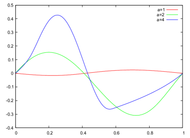
Figure 3. Plots of $\Psi(ah’;a,r)$ for three values of $a$. The variable $h’$ is on the horizontal axis.

In agreement with Lemma 4.2, we see that $\Psi(ah’;a,r)$ decays rapidly as $a\to 0$.

5. Numerical experiments

5.1. Classical Radon transform

In this subsection we experiment with the classical Radon transform (CRT), which integrates over lines:

(5.1) $$\hat{f}(\alpha,p)=\int_{S_{\alpha,p}}f(x)\text{d}x,\ \vec{\alpha}=(\cos\alpha,\sin\alpha),\ S_{\alpha,p}:=\{x\in\mathbb{R}^{2}:\alpha\cdot x=p\}.$$

Reconstruction uses (2.9):

(5.2) $$\begin{split}f_{\epsilon}^{\text{rec}}(x)=&-\frac{\Delta\alpha}{2\pi}\sum_{|\alpha_{k}|\leq\pi/2}\frac{1}{\pi}\int\frac{\partial_{p}\hat{f}_{\epsilon}(\alpha_{k},p)}{p-\mathcal{P}_{*}(x,\alpha_{k})}\text{d}p,\ \mathcal{P}_{*}(x,\alpha)\equiv\vec{\alpha}\cdot x,\\ \hat{f}_{\epsilon}(\alpha_{k},p)=&\int w_{\epsilon}(p-\rho)\hat{f}(\alpha_{k},\rho)\text{d}\rho,\ \alpha_{k}=-(\pi/2)+(\pi/N_{\alpha})(k+\delta),\end{split}$$

and $w$ is the same as in (4.7). The weights in both the Radon transform and the inversion formula are set to 1: $W(\alpha,p;x)\equiv 1$, $\omega(\alpha,x)\equiv 1$.

The function $f$ is the characteristic function of the disk centered at the origin with radius $r$. Thus, $\mathcal{S}=\{x\in\mathbb{R}^{2}:|x|=r\}$. By (2.2),

(5.3) $$|\text{d}H(y_{0})|=|\text{d}_{x}\mathcal{P}_{*}(\alpha_{\star},y_{0})|=|\alpha_{\star}|=1.$$

Therefore, by (2.3),

(5.4) $$M=-(\vec{\Theta}_{0}^{\perp}\cdot\partial_{y})^{2}H(y)|_{y=y_{0}}=1/r>0$$

is the curvature of $\mathcal{S}$ at $y_{0}$. Also, $\vec{\Theta}_{0}=\text{d}H(y_{0})$ points towards the center of curvature of $\mathcal{S}$ at $y_{0}$ (the center of the disk) .

At a given $x\not\in\mathcal{S}$, aliasing arises due to the parts of $\mathcal{S}$ where the lines $\mathcal{S}_{\alpha,p}\ni x$ are tangent to $\mathcal{S}$. For $|x|>r$, two such lines exist. We pick $x_{0}=(r,b)$ and find two pairs $(\alpha_{\star},p_{\star})$ with the required properties. Clearly, one of the pairs is $(\alpha_{\star}=\pi,p_{\star}=-r)$, and the other - $(\alpha_{\star}=2\tan^{-1}(b/r)-\pi,p_{\star}=-r)$. This choice of values of $(\alpha_{\star},p_{\star})$ ensures that $\mathcal{S}_{\alpha_{\star},p_{\star}+\delta}$, where $0<\delta\ll 1$, intersects $\mathcal{S}$ at two points (cf. the paragraph following (2.3)). See Figure 4, where the first pair (with $\alpha_{\star}=\pi$) is shown in red, and the second - in blue. Contributions coming from a neighborhood of each point of tangency $y_{0}$ are computed by (2.13) using the corresponding values of parameters (computed elsewhere in this subsection) and added. For reconstructions we use $r=5$ and $x_{0}=(5,7)$. To better illustrate the aliasing artifact we also reconstruct a small region of interest (ROI), which is a square centered at $x_{0}$ with side length $40\epsilon$.

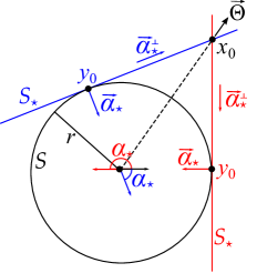
Figure 4. Illustration of various quantities used in the main formula (2.13) to predict aliasing from a disk in the case of the classical Radon transform.

For computations we also need $u_{0}$ and $\mu_{0}$ (cf. (2.13)). They follow easily from (2.6):

(5.5) $$u_{0}=\vec{\alpha}_{\star},\ \mu_{0}=\vec{\alpha}_{\star}^{\perp}\cdot(x_{0}-y_{0}),$$

where $y_{0}$ is the point where $\mathcal{S}_{\star}$ is tangent to $\mathcal{S}$. As is seen from Figure 4, $\mu_{0}=-|x_{0}-y_{0}|$ for the first (red) pair $(\alpha_{\star},p_{\star})$, and $\mu_{0}=|x_{0}-y_{0}|$ for the second (blue) pair.

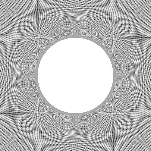
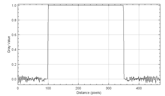
Figure 5. CRT reconstruction of the region $|x_{1}|,|x_{2}|\leq 10$: $\epsilon=0.02$, $N_{\alpha}=200$, $\delta=0.03$. Left: global reconstruction, right: profile of the reconstruction through the center.

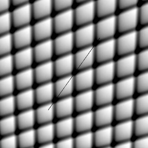
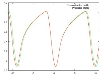
Figure 6. ROI CRT reconstruction: $\epsilon=0.02$, $N_{\alpha}=200$, $\delta=0.03$. The ROI is the square shown in Figure 5. Left: reconstructed ROI, right: reconstructed (green) and predicted (red) profiles along the line segment $x=x_{0}+\epsilon h\vec{\Theta}$, $|h|\leq 11$, shown on the left. The variable $h$ is on the horizontal axis.

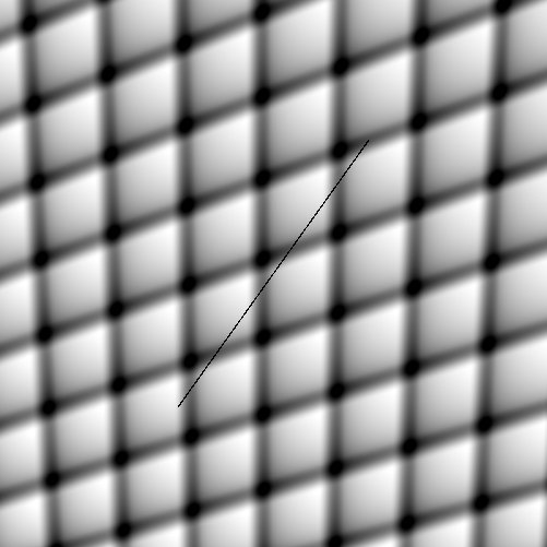
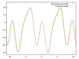
Figure 7. ROI CRT reconstruction: $\epsilon=0.02$, $N_{\alpha}=200$, $\delta=0.2$. The ROI is the square shown on the left in Figure 5. Left: reconstructed ROI, right: reconstructed (green) and predicted (red) profiles along the line segment $x=x_{0}+\epsilon h\vec{\Theta}$, $|h|\leq 11$, shown on the left. The variable $h$ is on the horizontal axis.

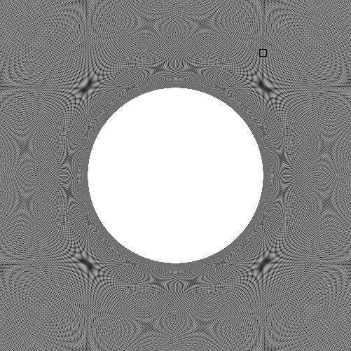
Figure 8. CRT reconstruction of the region $|x_{1}|,|x_{2}|\leq 10$: $\epsilon=0.01$, $N_{\alpha}=400$, $\delta=0.03$.

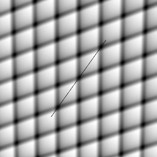
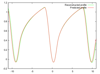
Figure 9. ROI CRT reconstruction: $\epsilon=0.01$, $N_{\alpha}=400$, $\delta=0.03$. The ROI is the square shown on the left in Figure 8. Left: reconstructed ROI, right: reconstructed (green) and predicted (red) profiles along the line segment $x=x_{0}+\epsilon h\vec{\Theta}$, $|h|\leq 11$, shown on the left. The variable $h$ is on the horizontal axis.

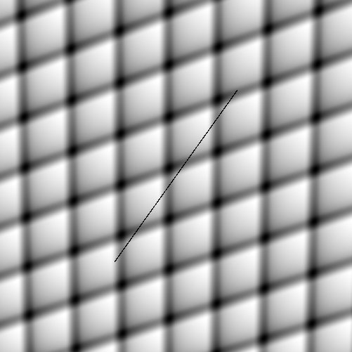
Figure 10. ROI CRT reconstruction: $\epsilon=0.01$, $N_{\alpha}=400$, $\delta=0.2$. The ROI is the square shown on the left in Figure 8. Left: reconstructed ROI, right: reconstructed (green) and predicted (red) profiles along the line segment $x=x_{0}+\epsilon h\vec{\Theta}$, $|h|\leq 11$, shown on the left. The variable $h$ is on the horizontal axis.

In the first experiment, $\epsilon=0.02$, $N_{\alpha}=200$, and in the second: $\epsilon=0.01$, $N_{\alpha}=400$. Since the direction $\alpha_{\star}=0$ is special, we use a non-zero shift $\delta$ in (5.2) for additional generality. The results are shown in Figures 5 – 10.

Figure 5 (left panel) shows the reconstructed region $|x_{1}|,|x_{2}|\leq 10$ with $\epsilon=0.02$ and $N_{\alpha}=200$. The left panel also shows the ROI (a small square). The right panel shows a line profile through the origin to confirm the accuracy of reconstruction. Figure 6 shows the reconstructed ROI with $\delta=0.03$. The right panel shows the profiles of the reconstructed difference $\epsilon^{-1/2}(f_{\epsilon}^{\text{rec}}(x)-f_{\epsilon}^{\text{rec}}(x_{0}))$ (green) and the prediction given by the main term on the right in (2.13) (red) along the line segment $x=x_{0}+\epsilon h\vec{\Theta}$, $|h|\leq 11$, where $\vec{\Theta}=x_{0}/|x_{0}|$. The line segment is indicated on the left panel. The values of $h$ are on the horizontal axis of the profile. From (5.5), the values of $u_{0}\cdot\check{x}$ used in (2.13) are given by $h\,\vec{\alpha}_{\star}\cdot\Theta$.

Similarly, Figure 7 shows the reconstructed ROI and line profiles for the same line segment when $\delta=0.2$.

Figure 8 shows the reconstructed region $|x_{1}|,|x_{2}|\leq 10$ with $\epsilon=0.01$ and $N_{\alpha}=400$. The ROI is indicated on the left panel. Recall that the size of the ROI is proportional to $\epsilon$. Figure 9 shows the ROI and the corresponding line profiles for $\delta=0.03$. Similarly, Figure 10 shows the reconstructed ROI and line profiles when $\delta=0.2$. In both cases, the vector $\vec{\Theta}$ and the range of $h$ that determine the line segment are the same as before.

Comparing Figure 6 with Figure 9 and Figure 7 with Figure 10, we see that reducing $\epsilon$ and $\Delta\alpha$ improves the match between the reconstruction and prediction.

5.2. Circular Radon transform

In this subsection we experiment with the generalized Radon transform (GRT), which integrates over circles with any radius $\rho>0$ and centers on the circle $|x|=R$:

(5.6) $$\begin{split}(\mathcal{R}f)(\alpha,\rho)=&\hat{f}(\alpha,\rho)=\int_{S_{\alpha,\rho}}f(x)\text{d}x,\ \vec{\alpha}=(\cos\alpha,\sin\alpha),\\ \mathcal{P}_{*}(\alpha,x):=&|x-R\vec{\alpha}|,\ S_{\alpha,\rho}:=\{x\in\mathbb{R}^{2}:|x-R\vec{\alpha}|=\rho\}.\end{split}$$

The value of $R$ is fixed. Therefore

(5.7) $$\begin{split}&\text{d}_{x}\mathcal{P}_{*}(\alpha,x)=\frac{x-R\vec{\alpha}}{|x-R\vec{\alpha}|},\ M=(1/\rho_{\star})-(\vec{\Theta}_{0}^{\perp}\cdot\partial_{y})^{2}H(y)|_{y=y_{0}}>0.\end{split}$$

In the computation of $M$ we used that $\text{d}_{x}\mathcal{P}_{*}(\alpha,x)=1$. Reconstruction is achieved using a straightforward modification of (2.9)

(5.8) $$\begin{split}f_{\epsilon}^{\text{rec}}(x)=&-\frac{\Delta\alpha}{2\pi}\sum_{\alpha_{k}\in\Omega}\frac{1}{\pi}\int\frac{\partial_{\rho}\hat{f}_{\epsilon}(\alpha_{k},\rho)}{p-\mathcal{P}_{*}(x,\alpha_{k})}\text{d}\rho,\\ \hat{f}(\alpha_{k},\rho)=&\int w_{\epsilon}(\rho-\rho’)\hat{f}(\alpha_{k},\rho’)\text{d}\rho’,\ \alpha_{k}=(2\pi/N_{\alpha})k,\ w(\rho)=(15/16)(1-\rho^{2})_{+}^{2},\end{split}$$

i.e. $w$ is the same as in (4.7). Clearly, the reconstruction is not theoretically exact anymore. But it preserves the strength of the singularities (in the Sobolev scale). Again, the weights in both the Radon transform and the inversion formula are set to 1: $W(\alpha,\rho;x)\equiv 1$, $\omega(\alpha,x)\equiv 1$.

The function $f$ is the characteristic function of the disk centered at $x_{c}$ with radius $r$. Thus, $\mathcal{S}=\{x\in\mathbb{R}^{2}:|x-x_{c}|=r\}$, see Figure 11 .

At a given $x_{0}$, aliasing arises due to the parts of $\mathcal{S}$ where various $\mathcal{S}_{\alpha,\rho}\ni x_{0}$ are tangent to $\mathcal{S}$. All such $(\alpha,\rho)$ are found by solving each of the two equations

(5.9) $$|x_{c}-R\vec{\alpha}|-|x_{0}-R\vec{\alpha}|=\pm r$$

for $\alpha$ and setting $\rho=|x_{0}-R\vec{\alpha}|$. Generally, up to four solutions $(\alpha,\rho)$ (i.e., up to four circles $\mathcal{S}_{\alpha,\rho}$) can exist. To simplify the experiment, we reverse the argument. We pick some pair $(\alpha_{\star},\rho_{\star})$ such that $\mathcal{S}_{\star}$ is tangent to $\mathcal{S}$ at some $y_{0}$, and then select some $x_{0}\in\mathcal{S}_{\star}$. To be specific, we select a ‘$+$’ in (5.9), i.e. $\rho_{\star}$ satisfies $|x_{c}-R\vec{\alpha}_{\star}|=r+\rho_{\star}$. This implies that $M=(1/r)+(1/\rho_{\star})$, and $\vec{\Theta}_{0}=(y_{0}-R\vec{\alpha}_{\star})/|y_{0}-R\vec{\alpha}_{\star}|$ points towards the center of curvature of $\mathcal{S}$ at $y_{0}$ (see Figure 11). Similarly to the classical Radon transform, our construction ensures that $\mathcal{S}_{\alpha_{\star},\rho_{\star}+\delta}$, where $0<\delta\ll 1$, intersects $\mathcal{S}$ at two points.

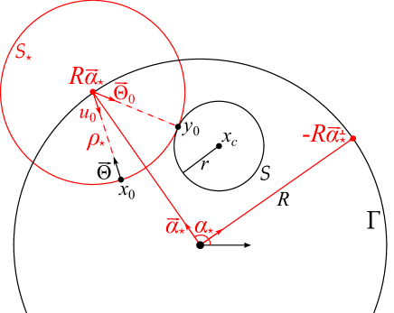
Figure 11. Illustration of various quantities used in the main formula (2.13) to predict aliasing from a disk in the case of the circular Radon transform.

To illustrate aliasing only from the place where $\mathcal{S}_{\star}$ is tangent to $\mathcal{S}$ we select $\Omega$ to be a sufficiently small neighborhood of $\alpha_{\star}$. Since $\mathcal{P}_{*}(\alpha,x)=|x-R\vec{\alpha}|$ and $\mathcal{P}(\alpha)=|x_{c}-R\vec{\alpha}|-r$, we find

(5.10) $$\begin{split}u_{0}=&\frac{x_{0}-R\vec{\alpha}_{\star}}{|x_{0}-R\vec{\alpha}_{\star}|},\\ \mu_{0}=&-R\vec{\alpha}_{\star}^{\perp}\cdot(u_{0}-\vec{\Theta}_{0})=-(R/\rho_{\star})\vec{\alpha}_{\star}\cdot(x_{0}-y_{0}),\end{split}$$

see Figure 11.

For reconstructions we use

(5.11) $$\begin{split}&R=5,\ x_{c}=(1,1),\ r=2,\ (\alpha_{\star},\rho_{\star})=(0.53\pi,2.24),\ x_{0}=(-1.42,2.95),\\ &\Omega:=[\alpha_{\star}-\pi/4,\alpha_{\star}+\pi/4].\end{split}$$

In the first reconstruction, $\epsilon=10^{-2}$, $N_{\alpha}=500$, and in the second: $\epsilon=0.5\cdot 10^{-2}$, $N_{\alpha}=1000$. The results are shown in Figures 12 and 13, respectively. The left panels show the limited angle reconstruction of the region $|x_{1}|,|x_{2}|\leq 4$. The middle panels show the limited angle reconstruction of an ROI. The ROI is a small square centered at $x_{0}$ with side length $40\epsilon$, the ROI is shown on the left panel. The right panels show the profiles of the reconstructed difference $\epsilon^{-1/2}(f_{\epsilon}^{\text{rec}}(x)-f_{\epsilon}^{\text{rec}}(x_{0}))$ (green) and the prediction given by the main term on the right in (2.13) (red) along the line segment $x=x_{0}+\epsilon h\vec{\Theta}$, $|h|\leq 6$, shown in the middle panel. The values of $h$ are on the horizontal axis of the profiles. The unit vector $\vec{\Theta}$ is chosen to be orthogonal to $\mathcal{S}_{\star}$ at $x_{0}$ (i.e., $\vec{\Theta}$ and $u_{0}$ are parallel, see Figure 11 ). In the experiments we set $\vec{\Theta}=-u_{0}$. As is seen, reducing $\epsilon$ and $\Delta\alpha$ improves the match between the reconstruction and prediction.

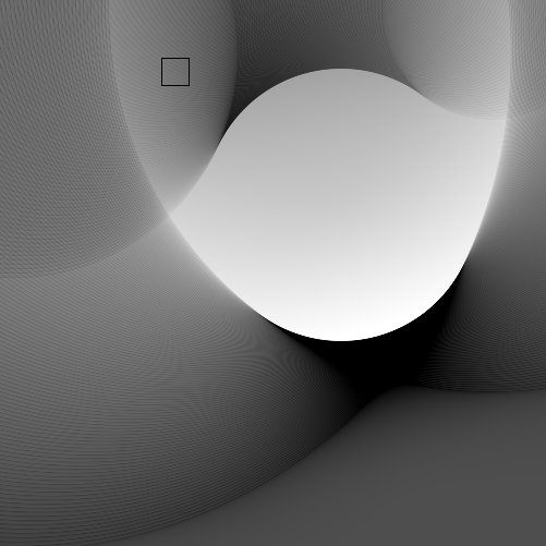
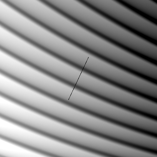
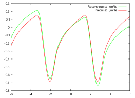
Figure 12. Limited angle GRT reconstruction: $\epsilon=0.01$, $N_{\alpha}=500$. Left: global reconstruction, middle: reconstruction inside the square ROI shown on the left, right: profiles of the reconstruction (green) and prediction (red) along the line segment $x=x_{0}+\epsilon h\vec{\Theta}$, $|h|\leq 6$, shown in the middle. The variable $h$ is on the horizontal axis.

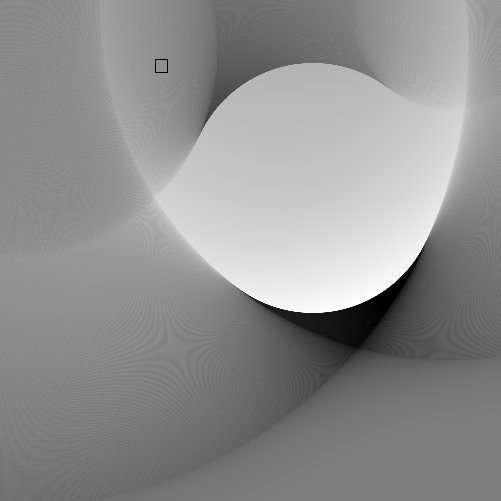
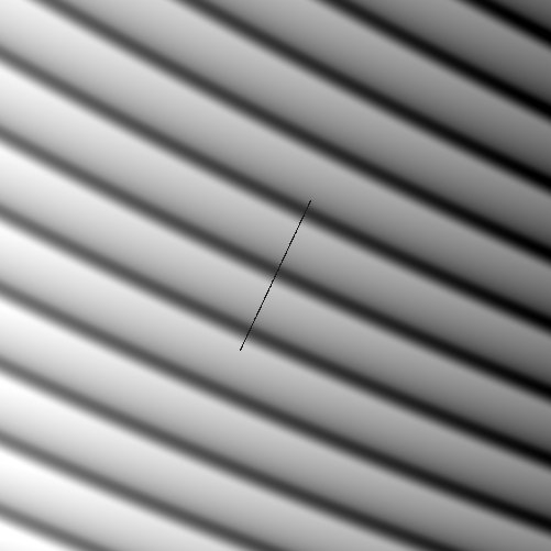
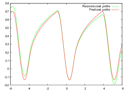
Figure 13. Limited angle GRT reconstruction: $\epsilon=0.005$, $N_{\alpha}=1000$. Left: global reconstruction, middle: reconstruction inside the square ROI shown on the left, right: profiles of the reconstruction (green) and prediction (red) along the line segment $x=x_{0}+\epsilon h\vec{\Theta}$, $|h|\leq 6$, shown in the middle. The variable $h$ is on the horizontal axis.

Appendix A Proofs of lemmas

A.1. Proof of Lemma 2.2

The property $\mathcal{P}(\alpha_{\star})=p_{\star}$ follows from assumption 2.1(2). Recall that $H(y)=0$ is a local equation of $\mathcal{S}$ (cf. (2.2) and the paragraph preceding it). To find $\mathcal{P}(\alpha)$, we solve

(A.1) $$H(y)=0,\ \lambda\text{d}H(y)=\text{d}_{y}\mathcal{P}_{*}(\alpha,y)$$

for $y\in\mathcal{S}$ and $\lambda$ in terms of $\alpha$ near $({\color[rgb]{0,0,0}\lambda=1,}y=y_{0},\alpha=\alpha_{\star})$ and then set $\mathcal{P}(\alpha)=\mathcal{P}_{*}(\alpha,y(\alpha))$. Assumptions 2.1(1, 2, 4) and the Implicit Function Theorem imply that $y(\alpha)$ and, therefore, $\mathcal{P}(\alpha)$ are smooth in a small neighborhood $\Omega\ni\alpha_{\star}$. Since $y’(\alpha)$ is tangent to $\mathcal{S}$, using the second equation in (A.1) gives $\mathcal{P}’(\alpha_{\star})=\partial_{\alpha}\mathcal{P}_{*}(\alpha_{\star},y_{0})$.

A.2. Proof of Lemma 3.1

Denote

(A.2) $$H(x,\alpha,\epsilon):=\frac{\mathcal{P}_{*}(\alpha,x)-\mathcal{P}(\alpha)}{\epsilon},\ x=x_{0}+\epsilon\check{x},\alpha\in\Omega.$$

Since $\mu_{0}\not=0$ (cf. (2.6)), we have $|\mathcal{P}_{*}(\alpha,x_{0})-\mathcal{P}(\alpha)|\geq c|\alpha-\alpha_{\star}|$ for any $\alpha\in\Omega$ and some $c>0$. Hence

(A.3) $$|H(x,\alpha_{k},\epsilon)|\geq c_{1}|k-k_{\star}|,\text{ for all }|\check{x}|\leq c,\alpha_{k}\in\Omega,{\color[rgb]{0,0,0}|k-k_{\star}|\geq c_{2},}$$

for some $c,c_{1},c_{2}>0$, and all $\epsilon>0$ sufficiently small. From (3.5),

(A.4) $$\begin{split}&f_{\epsilon}^{\text{rec-1}}(x_{0}+\epsilon\check{x})-f_{\epsilon}^{\text{rec-1}}(x_{0})=-\frac{\Delta\alpha}{2\pi\epsilon^{1/2}}\bigl{(}J+O(\epsilon^{1/2})\bigr{)},\\ &J:=\sum_{\alpha_{k}\in\Omega}\omega(\alpha_{k},x_{0})\varphi_{1}(\alpha_{k})\left[\psi\left(H(x_{0}+\epsilon\check{x},\alpha_{k},\epsilon)\right)-\psi\left(H(x_{0},\alpha_{k},\epsilon)\right)\right].\end{split}$$

The $O(\epsilon^{1/2})$ term in parentheses on the right in (A.4) denotes the contribution, which arises due to the $x$-dependence of $\omega$ in (3.5). Here we use (3.6) with $n=0$, (A.3), and that for some $c$ and all $\check{x}$ in a bounded set:

(A.5) $$|\omega(\alpha,x_{0}+\epsilon\check{x})-\omega(\alpha,x_{0})|\leq c\epsilon,\ |\varphi_{1}(\alpha)|\leq c,\ \alpha\in\Omega,$$

hence

(A.6) $$O(\epsilon)\biggl{(}O(1)+\sum_{c_{2}\leq|k-k_{\star}|\leq O(1/\epsilon)}|k-k_{\star}|^{-1/2}\biggr{)}=O(\epsilon^{1/2}).$$

From (2.6),

(A.7) $$\begin{split}H(x_{0}+\epsilon\check{x},\alpha,\epsilon)&={\color[rgb]{0,0,0}H(x_{0},\alpha,\epsilon)+\text{d}_{x}\mathcal{P}_{*}(\alpha,x_{0})\check{x}+O(\epsilon)}\\ &=H(x_{0},\alpha,\epsilon)+u_{0}\cdot\check{x}+O(\epsilon+|\alpha-\alpha_{\star}|).\end{split}$$

Also, $|\omega(x_{0},\alpha)\varphi_{1}(\alpha)|\leq c$ for some $c$ and all $\alpha\in\Omega$. Therefore, by (3.6) with $n=1$ and (A.3),

(A.8) $$\begin{split}\sum_{\alpha_{k}\in\Omega}&\omega(\alpha_{k},x_{0})\varphi_{1}(\alpha_{k})\bigl{[}\psi(H(x_{0}+\epsilon\check{x},\alpha_{k},\epsilon))-\psi(H(x_{0},\alpha_{k},\epsilon)+u_{0}\cdot\check{x})\bigr{]}\\ &=\sum_{|k|\leq O(1/\epsilon)}\psi’(H(x_{0},\alpha_{k},\epsilon)+O(1))O(\epsilon+\epsilon|k-k_{\star}|)\\ &=O(\epsilon)\biggl{(}1+\sum_{{\color[rgb]{0,0,0}c_{2}\leq}|k-k_{\star}|\leq O(1/\epsilon)}\frac{1+|k-k_{\star}|}{|k-k_{\star}|^{3/2}}\biggr{)}=O(\epsilon^{1/2}).\end{split}$$

Here we use that $w’\in L^{q}(\mathbb{R})$, $q>2$ (see assumption 2.4(1)), so $\psi’$ is continuous. This shows that if $w$ does not have the required smoothness (e.g., if $w$ is the characteristic function of a detector pixel), the magnitude of the expression in (A.8) may turn out to be much larger, leading to a slower rate of convergence in Theorem 2.5 (or even to a breakdown of the convergence altogether).

From (A.4), (A.7), and (A.8),

(A.9) $$\begin{split}&J=\sum_{\alpha_{k}\in\Omega}\omega(\alpha_{k},x_{0})\varphi_{1}(\alpha_{k})\Delta\psi(H(x_{0},\alpha_{k},\epsilon))+O(\epsilon^{1/2}),\\ &\Delta\psi(t):=\psi(t+u_{0}\cdot\check{x})-\psi(t).\end{split}$$

Furthermore,

(A.10) $$H(x_{0},\alpha_{k},\epsilon)=\mu_{0}\frac{\alpha_{k}-\alpha_{\star}}{\epsilon}+R_{k},\ R_{k}=O(\epsilon(k-k_{\star})^{2}).$$

Denote, for simplicity, $a_{k}=\mu_{0}\kappa(k-k_{\star})$. Then

(A.11) $$\Delta\psi(a_{k}+R_{k})-\Delta\psi(a_{k})=R_{k}\Delta\psi’(a_{k}+\xi_{k}),$$

where $|\xi_{k}|\leq|R_{k}|$. We can assume that $\Omega$ is sufficiently small, so that

(A.12) $$|\mu_{0}(\alpha_{k}-\alpha_{\star})+\epsilon R_{k}|\geq c|\alpha_{k}-\alpha_{\star}|,\ \forall\alpha_{k}\in\Omega,$$

for some $c>0$. Dividing by $\epsilon$ implies

(A.13) $$\left|a_{k}+R_{k}\right|\geq c\kappa|k-k_{\star}|,\ \forall\alpha_{k}\in\Omega,$$

with the same $c$. Using (3.6) with $n=2$ gives

(A.14) $$\begin{split}\sum_{{\color[rgb]{0,0,0}c\leq}|k-k_{\star}|\leq O(1/\epsilon)}&\omega(\alpha_{k},x_{0})\varphi_{1}(\alpha_{k})\bigl{[}\Delta\psi(a_{k}+R_{k})-\Delta\psi(a_{k})\bigr{]}\\ &=\sum_{{\color[rgb]{0,0,0}c\leq}|k-k_{\star}|\leq O(1/\epsilon)}\frac{O(\epsilon|k-k_{\star}|^{2})}{1+|k-k_{\star}|^{5/2}}=O(\epsilon^{1/2}),\end{split}$$

for some $c>0$ sufficiently large. The requirement $|k-k_{\star}|\geq c$ is needed, because $\psi^{\prime\prime}(\hat{q})$, on which the estimate (A.14) is based, may not exist for $\hat{q}$ in a compact set when $w’\in L^{q}$. To estimate the remaining finitely many terms without appealing to the second derivative we write

(A.15) $$\begin{split}&\Delta\psi(a_{k}+R_{k})-\Delta\psi(a_{k})\\ &=\bigl{[}\psi(a_{k}+u_{0}\cdot\check{x}+R_{k})-\psi(a_{k}+u_{0}\cdot\check{x})\bigr{]}-\bigl{[}\psi(a_{k}+R_{k})-\psi(a_{k})\bigr{]}\\ &=O(\epsilon),\ |k-k_{\star}|\leq c.\end{split}$$

This follows, because $\psi’$ is continuous on all of $\mathbb{R}$, and $R_{k}=O(\epsilon)$ whenever $|k-k_{\star}|\leq c$ (cf. (A.10)). This is another place where we use that $w’\in L^{q}$. If $w$ is not sufficiently smooth, the quantity in (A.15) may turn out to be much larger.

It is clear that all the big-$O$ terms are uniform with respect to $\check{x}$ (and, hence, $h$) restricted to a bounded set. Combining (A.4), (A.9), (A.14), and (A.15) finishes the proof.

A.3. Proof of Lemma 3.2

Denote

(A.16) $$J:=\int s^{-1}\left[\varphi_{3}’(s+q+\Delta q)-\varphi_{3}’(s+q)\right]\text{d}s,$$

where we omitted the dependence on $\alpha$ for simplicity. All the big-$O$ terms in this subsection are uniform with respect to $\alpha\in\Omega$. Restricting the integral in (A.16) to $|s|\leq 1$ we find

(A.17) $$J_{1}:=\int_{|s|\leq 1}s^{-1}\left(\left[\varphi_{3}’(s+q+\Delta q)-\varphi_{3}’(q+\Delta q)\right]-\left[\varphi_{3}’(s+q)-\varphi_{3}’(q)\right]\right)\text{d}s.$$

Clearly, $J_{1}=O(|\Delta q|)$ uniformly in $|q|\leq c$. Here we have used that $\varphi_{3}$ is smooth, so its third order derivative is bounded on compact sets. By (3.18), $\varphi_{3}^{\prime\prime}(p)=O(|p|^{-3/2}),\ p\to\infty$. Hence

(A.18) $$J_{2}:=\int_{|s|\geq 1}s^{-1}\left[\varphi_{3}’(s+q+\Delta q)-\varphi_{3}’(s+q)\right]\text{d}s=O(|\Delta q|)$$

uniformly in $|q|\leq c$. Combining the estimates for $J_{1,2}$ proves the lemma.

A.4. Proof of Lemma 4.3

The Euler-MacLauren formula reads as follows [38, eq. (25.7)]:

(A.19) $$\begin{split}\sum_{k=a}^{b-1}f(k)=&\int_{a}^{b}f(t)\text{d}t+\sum_{m=1}^{N’}\frac{b_{m}}{m!}(f^{(m-1)}(b)-f^{(m-1)}(a))\\ &-\int_{a}^{b}\frac{B_{N’}(\{1-t\})}{N’!}f^{(N’)}(t)\text{d}t.\end{split}$$

Here $b>a$ are integers, $B_{m}$ and $b_{m}$ are Bernoulli polynomials and numbers, respectively, $\{t\}=t-\lfloor t\rfloor$ is the fractional part of $t\in\mathbb{R}$, and $\lfloor t\rfloor$ is the floor function, i.e. the largest integer not exceeding $t$.

Substituting $f(t)=g(\epsilon t)$, taking the limit as $a\to-\infty$, $b\to\infty$ (which is allowed due to the decay of $g$ and its derivatives), changing variables $\tau=\epsilon t$, and using that $g^{(N’)}\in L^{1}(\mathbb{R})$, we finish the proof.

References

- [1] C. L. Epstein, Introduction to the mathematics of medical imaging. Philadelphia: SIAM, second ed., 2008.
- [2] B. Li, G. B. Avinash, and J. Hsieh, “Resolution and noise trade-off analysis for volumetric CT,” Medical Physics, vol. 34, no. 10, pp. 3732–3738, 2007.
- [3] R. Grimmer, J. Krause, M. Karolczak, R. Lapp, and M. Kachelriess, “Assessment of spatial resolution in CT,” IEEE Nuclear Science Symposium Conference Record, pp. 5562–5566, 2008.
- [4] S. N. Friedman, G. S. Fung, J. H. Siewerdsen, and B. M. Tsui, “A simple approach to measure computed tomography (CT) modulation transfer function (MTF) and noise-power spectrum (NPS) using the American College of Radiology (ACR) accreditation phantom,” Medical Physics, vol. 40, no. 5, pp. 1–9, 2013.
- [5] H. Kruse, “Resolution of Reconstruction Methods in Computerized Tomography,” SIAM Journal on Scientific and Statistical Computing, vol. 10, pp. 447–474, 1989.
- [6] L. Desbat, “Efficient sampling on coarse grids in tomography,” Inverse Problems, vol. 9, pp. 251–269, 1993.
- [7] F. Natterer, “Sampling in Fan Beam Tomography,” SIAM Journal on Applied Mathematics, vol. 53, pp. 358–380, 1993.
- [8] F. Natterer, “Sampling and resolution in CT,” in Proceedings of the Fourth International Symposium (CT-93): Novosibirsk, 1993 (M. M. Lavrentév, ed.), pp. 343–354, Utrecht: VSP, 1995.
- [9] V. P. Palamodov, “Localization of harmonic decomposition of the Radon transform,” Inverse Problems, vol. 11, pp. 1025–1030, 1995.
- [10] A. Caponnetto and M. Bertero, “Tomography with a finite set of projections: singular value decomposition and resolution,” IEEE Transactions on Information Theory, vol. 13, pp. 1191–1205, 1997.
- [11] A. Faridani and E. Ritman, “High-resolution computed tomography from efficient sampling,” Inverse Problems, vol. 16, pp. 635–650, 2000.
- [12] A. Faridani, “Sampling theory and parallel-beam tomography,” in Sampling, wavelets, and tomography, vol. 63 of Applied and Numerical Harmonic Analysis, pp. 225–254, Boston, MA: Birkhauser Boston, 2004.
- [13] A. Rieder and A. Schneck, “Optimality of the fully discrete filtered backprojection algorithm for tomographic inversion,” Numerische Mathematik, vol. 108, pp. 151–175, 2007.
- [14] S. H. Izen, “Sampling in Flat Detector Fan Beam Tomography,” SIAM Journal on Applied Mathematics, vol. 72, pp. 61–84, 2012.
- [15] P. Stefanov, “Semiclassical sampling and discretization of certain linear inverse problems,” SIAM Journal of Mathematical Analysis, vol. 52, pp. 5554–5597, 2020.
- [16] F. Monard and P. Stefanov, “Sampling the X-ray transform on simple surfaces,” ArXiv ID:2110.05761, 2021.
- [17] P. Stefanov, “The Radon transform with finitely many angles,” arXiv:2208.05936v1, pp. 1–30, 2022.
- [18] A. Katsevich, “A local approach to resolution analysis of image reconstruction in tomography,” SIAM Journal on Applied Mathematics, vol. 77, no. 5, pp. 1706–1732, 2017.
- [19] A. Katsevich, “Analysis of reconstruction from discrete Radon transform data in when the function has jump discontinuities,” SIAM Journal on Applied Mathematics, vol. 79, pp. 1607–1626, 2019.
- [20] A. Katsevich, “Analysis of resolution of tomographic-type reconstruction from discrete data for a class of distributions,” Inverse Problems, vol. 36, no. 12, 2020.
- [21] A. Katsevich, “Resolution analysis of inverting the generalized Radon transform from discrete data in ,” SIAM Journal of Mathematical Analysis, vol. 52, no. 4, pp. 3990–4021, 2020.
- [22] A. Katsevich, “Resolution analysis of inverting the generalized -dimensional Radon transform in from discrete data,” Journal of Fourier Analysis and Applications, vol. 29, art. 6, 2023.
- [23] A. Katsevich, “Resolution of 2D reconstruction of functions with nonsmooth edges from discrete Radon transform data,” SIAM Journal on Applied Mathematics, vol. to appear, 2023.
- [24] A. Katsevich, “Novel resolution analysis for the Radon transform in for functions with rough edges,” SIAM Journal of Mathematical Analysis, vol. to appear, 2023.
- [25] P. M. Joseph and R. A. Schulz, “View sampling requirements in fan beam computed tomography,” Medical Physics, vol. 7, no. 6, pp. 692–702, 1980.
- [26] P. Kuchment, “Generalized transforms of Radon type and their applications,” in The Radon Transform, Inverse Problems, and Tomography (G. Ólafsson and E. T. Quinto, eds.), pp. 67–91, Providence, R.I.: American Mathematical Society, 2005.
- [27] G. Ambartsoumian and E. T. Quinto, “Generalized Radon transforms and applications in tomography,” Inverse Problems, vol. 36, no. 2, p. 020301, 2020.
- [28] F. Natterer, The Mathematics of Computerized Tomography. Philadelphia: SIAM, 2001.
- [29] G. Beylkin, “The inversion problem and applications of the generalized Radon transform,” 1984.
- [30] A. Katsevich, “An accurate approximate algorithm for motion compensation in two-dimensional tomography,” Inverse Problems, vol. 26, 2010.
- [31] E. T. Quinto, “The dependence of the generalized Radon transforms on defining measures,” Transactions of the American Mathematical Society, vol. 257, pp. 331–346, 1980.
- [32] A. G. Ramm and A. I. Zaslavsky, “Singularities of the Radon transform,” Bull. Amer. Math. Soc., vol. 25, pp. 109–115, 1993.
- [33] A. G. Ramm and A. I. Zaslavsky, “Reconstructing singularities of a function given its Radon transform,” Math. and Comput. Modelling, vol. 18, no. 1, pp. 109–138, 1993.
- [34] N. I. Muskhelishvili, Singular Integral Equations. Boundary problems of functions theory and their applications to mathematical physics. Dordrecht: Springer, 1958.
- [35] W. Rudin, Real and Complex Analysis. London: McGraw-Hill, 1970.
- [36] F. D. Gakhov, Boundary Value Problems. Oxford: Pergamon Press, 1966.
- [37] A. P. Prudnikov, Y. A. Brychkov, and O. I. Marichev, Integrals and series. Volume 1. Elementary functions. New York: Gordon and Breach, 1986.
- [38] V. Kac and P. Cheung, Quantum Calculus. New York, NY: Springer, 2002.
- [39] G. Nemes, “Error bounds for the asymptotic expansion of the Hurwitz zeta function,” Proceedings of the Royal Society A: Mathematical, Physical and Engineering Sciences, vol. 473, no. 2203, 2017.