Hyper-parameter Tuning for
Fair Classification without Sensitive Attribute Access

Abstract

Fair machine learning methods seek to train models that balance model performance across demographic subgroups defined over sensitive attributes like race and gender. Although sensitive attributes are typically assumed to be known during training, they may not be available in practice due to privacy and other logistical concerns. Recent work has sought to train fair models without sensitive attributes on training data. However, these methods need extensive hyper-parameter tuning to achieve good results, and hence assume that sensitive attributes are known on validation data. However, this assumption too might not be practical. Here, we propose Antigone, a framework to train fair classifiers without access to sensitive attributes on either training or validation data. Instead, we generate pseudo sensitive attributes on the validation data by training a biased classifier and using the classifier’s incorrectly (correctly) labeled examples as proxies for minority (majority) groups. Since fairness metrics like demographic parity, equal opportunity and subgroup accuracy can be estimated to within a proportionality constant even with noisy sensitive attribute information, we show theoretically and empirically that these proxy labels can be used to maximize fairness under average accuracy constraints. Key to our results is a principled approach to select the hyper-parameters of the biased classifier in a completely unsupervised fashion (meaning without access to ground truth sensitive attributes) that minimizes the gap between fairness estimated using noisy versus ground-truth sensitive labels.

1 Introduction

Deep neural networks have achieved state-of-the-art accuracy on a wide range of real-world tasks. But, prior work (Hovy & Søgaard, 2015; Oren et al., 2019; Hashimoto et al., 2018a) has found that state-of-the-art networks exhibit unintended biases towards specific population groups, especially harming minority groups. Seminal work by (Buolamwini & Gebru, 2018) demonstrated, for instance, that commercial face recognition systems had lower accuracy on darker skinned women than other groups. A body of work has sought to design fair machine learning algorithms that account for a model’s performance on a per-group basis (Prost et al., 2019; Liu et al., 2021; Sohoni et al., 2020).

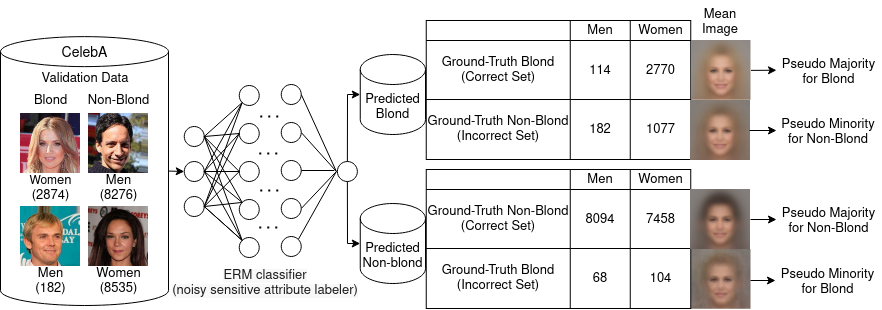
Figure 1: Antigone on CelebA dataset with hair color as target label and gender as (unknown) sensitive attribute. Blond men are discriminated against. Correspondingly, the mean image of the Blond class’ incorrect (row 4) has more male features than that of its correct set (row 1), reflecting this bias. Similarly, a bias against non-blond women is also reflected.

Much of the prior work assumes that demographic attributes like gender and race on which we seek to train fair models, referred to as sensitive attributes, are available on training and validation data (Sagawa* et al., 2020; Prost et al., 2019). However, there is a growing body of literature (Veale & Binns, 2017; Holstein et al., 2019) highlighting real-world settings in which sensitive attributes may not be available. For example, data subjects may abstain from providing sensitive information for privacy reasons or to eschew potential discrimination in the future (Markos et al., 2017). Alternately, the attributes on which the model discriminates might not be known or available during training and only identified post-deployment (Citron & Pasquale, 2014; Pasquale, 2015). For instance, recent work shows that fair natural language processing models trained on western datasets discriminate based on last names when re-contextualized to geo-cultural settings like India (Bhatt et al., 2022). Similarly, Nikon’s face detection models were reported as repeatedly identify Asian faces as blinking, a bias that was only identified retrospectively (Leslie, 2020). Unfortunately, by this point at least some harm is already incurred.

Hence, recent work seeks to train fair classifiers without access to sensitive attributes on the training set (Liu et al., 2021; Creager et al., 2021; Nam et al., 2020; Hashimoto et al., 2018a). Although the details vary, these methods all work in two stages. In the first stage, sub-groups in the training data potentially being discriminated against are identified. In the second, a fair training procedure is used to train a fair model with respect to these sub-groups. For example, JTT’s (Liu et al., 2021) stage 1 uses mis-classified examples of a standard empirical risk minimization (ERM) model as a proxy for minority sub-groups. In stage 2, JTT retrains the model by up-weighting these mis-classified examples.

However, Liu et al., (2021) have shown that these methods are highly sensitive to choice of hyper-parameters; the up-weighting factor in JTT, for example, can have a significant impact on the resulting model’s fairness. JTTs results without proper hyper-parameter tuning can be even less fair that standard ERM (Liu et al., 2021). Therefore, JTT and other methods (except for GEORGE (Sohoni et al., 2020)) assume access to sensitive attributes on the validation data for hyper-parameter tuning.

However, sensitive information on the validation dataset may not be available for the same reasons they are hard to acquire on training data.

In this paper, we propose Antigone, a principled approach that enables hyper-parameter tuning for fairness without access to sensitive attributes on validation data.  Antigone can be used in conjunction with prior methods like JTT and GEORGE that train fair models without sensitive attributes on training data (Liu et al., 2021), and for several fairness metrics including demographic parity, equal opportunity and worst sub-group accuracy.

Antigone builds on the same intuition as in prior work: mis-classified examples of a model trained with standard ERM loss serve as an effective proxy for minority groups. Accordingly, Antigone uses an ERM classifier to obtain pseudo sensitive attribute labels on the validation dataset using correctly and incorrectly classified validation data as proxies for majority and minority groups, respectively. That is, the ERM classifier can be viewed as a noisy sensitive attribute labeler on the validation dataset. But this raises a key question: how do we select the hyper-parameters of the noisy sensitive attribute labeler?

Intuitively, to obtain accurate sensitive attribute labels, we seek to maximize the fraction of true minority (majority) samples in the ERM classifier’s incorrect (correct) set. In other words, the sensitive attribute labels of the ERM classifier will be accurate if (perhaps counter-intuitively) the classifier is itself biased. Figure 1 illustrates this intuition using the CelebA dataset in which blond men are discriminated against; hence, the incorrect set for the blond class has a greater fraction of men than its correct set. Since the classifier’s bias cannot be measured directly, Antigone uses the distance between the data distributions of the correct and incorrect sets as a proxy. Specifically, Antigone uses the Euclidean distance between the means (EDM) of the two sets as a distance measure. The mean images of each set for CelebA are shown in Figure 1 and visually capture the ERM model’s biases.

We provide theoretical justification for Antigone in an idealized setting in which a fraction of sensitive attribute labels from the minority group are contaminated with labels from majority group (and vice-versa). This is referred to as the mutually contaminated (MC) noise model in literature (Scott et al., 2013), and prior work shows that common fairness metrics can be estimated up to a proportionality constant under this model (Lamy et al., 2019). We show that maximizing Antigone’s EDM metric equivalently maximizes this proportionality constant, thus providing the most reliable estimates of fairness.

We evaluate Antigone in conjunction with JTT (Liu et al., 2021) and GEORGE (Sohoni et al., 2020) on the CelebA, Waterbirds and UCI Adult datasets using demographic parity, equal opportunity, and worst subgroup accuracy as fairness metrics. Empirically, we find that (1) Antigone produces more accurate sensitive attribute labels on validation data compared to GEORGE; (2) used with JTT, Antigone comes close to matching the fairness of JTT with ground-truth sensitive attribute labels on validation data; and (3) improves fairness of GEORGE when its sensitive attribute labels are replaced with Antigone’s. Ablation studies demonstrate the effectiveness of Antigone’s EDM metric versus alternatives.

2 Proposed Methodology

We now describe Antigone, starting with the problem formulation (Section 2.1) followed by a description of the Antigone algorithm (Section 2.2).

2.1 Problem Setup

Consider a data distribution over set $\mathcal{D}=\mathcal{X}\times\mathcal{A}\times\mathcal{Y}$, the product of input data ($\mathcal{X}$), sensitive attributes ($\mathcal{A}$) and target labels ($\mathcal{Y}$) triplets. We are given a training set $D^{tr}=\{x^{tr}_{i},a^{tr}_{i},y^{tr}_{i}\}_{i=1}^{N^{tr}}$ with $N^{tr}$ training samples, and a validation set $D^{val}=\{x^{val}_{i},a^{val}_{i},y^{val}_{i}\}_{i=1}^{N^{val}}$ with $N^{val}$ validation samples. We will assume binary sensitive attributes ($\mathcal{A}\in\{0,1\}$) and target labels ($\mathcal{Y}\in\{0,1\}$). We note that for now Antigone is limited to binary sensitive attributes, but can be extended to multiple target labels.

We seek to train a machine learning model, say a deep neural network (DNN), which can be represented as a parameterized function $f_{\theta}:\mathcal{X}\rightarrow\mathcal{Y}\in\{0,1\}$, where $\theta\in\Theta$ are the trainable parameters, e.g., DNN weights and biases.

Standard fairness unaware empirical risk minimization (ERM) optimizes over trainable parameters $\theta$ to minimize average loss $\mathcal{L}_{ERM}$:

$$\mathcal{L}_{ERM}=-\frac{1}{N^{tr}}\sum_{i=1}^{N}l(x^{tr}_{i},y^{tr}_{i}),$$ (1)

on $D^{tr}$, where $l(x_{i},y_{i})$ is the binary cross-entropy loss.

Optimized model parameters $\theta^{*}$ are obtained by invoking a training algorithm, for instance stochastic gradient descent (SGD), on the training dataset and model, i.e., $\theta^{*,\gamma}=\mathcal{M}^{ERM}(D^{tr},f_{\theta},\gamma)$, where $\gamma\in\Gamma$ are hyper-parameters of the training algorithm including learning rate, training epochs etc. Hyper-parameters are tuned by evaluating models $f_{\theta^{*,\gamma}}$ for all $\gamma\in\Gamma$ on $D^{val}$ and picking the best model. More sophisticated algorithms like Bayesian optimization can also be used.

Now, we review three commonly used fairness metrics that we account for in this paper.

Demographic parity (DP):

DP requires the model’s outcomes to be independent of sensitive attribute. In practice, we seek to minimize the demographic parity gap:

$$\Delta^{DP}_{\theta}=\mathbb{P}[f_{\theta}(X)=1|A=1]-\\ \mathbb{P}[f_{\theta}(X)=1|A=0]$$ (2)

Equal opportunity (EO):

EO aims to equalize only the model’s true positive rates across sensitive attributes. In practice, we seek to minimize

$$\begin{split}\Delta^{EO}_{\theta}=\mathbb{P}[f_{\theta}(X)=1|A=1,Y=1]-\\ \mathbb{P}[f_{\theta}(X)=1|A=0,Y=1]\end{split}$$ (3)

Worst-group accuracy (WGA):

WGA seeks to maximize the minimum accuracy over all sub-groups (over sensitive attributes and target labels). That is, we seek to maximize:

$$WGA_{\theta}=\min_{a\in\{0,1\},y\in\{0,1\}}\mathbb{P}[f(x)=y|A=a,Y=y]$$ (4)

In all three settings, we seek to train models that optimize fairness under a constraint on average target label accuracy, i.e., accuracy in predicting the target label. For example, for equal opportunity, we seek $\theta^{*}=\arg\min_{\theta\in\Theta}\Delta^{EO}_{\theta}$ such that $\mathbb{P}[f_{\theta}(x)=Y]\in[Acc^{thr}_{lower},Acc^{thr}_{upper})$, where $Acc^{thr}_{lower}$ and $Acc^{thr}_{upper}$ are user-specified lower and upper bounds on target label accuracies, respectively.

2.2 Antigone Algorithm

We now describe the Antigone algorithm which consists of three main steps. In step 1, we train multiple intentionally biased ERM models that each provide pseudo sensitive attribute labels on validation data. We view each model as a noisy sensitive attribute labeller on the validation set. In step 2, we use the proposed EDM metric to pick a noisy labeller from step 1 with the least noise. Finally, in step 3, we use the labelled validation set from step 2 to tune the hyper-parameters of methods like JTT that train fair classifiers without sensitive attributes on training data.

Step 1: Generating sensitive attribute labels on validation set.

In step 1, we use the training dataset and standard ERM training to obtain a set of classifiers, $\theta^{*,\gamma}=\mathcal{M}^{ERM}(D^{tr},f_{\theta},\gamma)$, each corresponding to a different value of training hyper-parameters $\gamma\in\Gamma$. As we discuss in Section 2.1, these include learning rate, weight decay and number of training epochs. Each classifier, which predicts the target label for a given input, generates a validation set with noisy pseudo sensitive attribute labels as follows:

$$D^{val,\gamma}_{{\color[rgb]{0,0,0}noisy}}=\{x^{val}_{i},a^{val,\gamma}_{i},y^{val}_{i}\}_{i=1}^{N^{val}}\quad\forall\gamma\in\Gamma$$ (5)

where:

$$a^{val,\gamma}_{i}=\begin{cases}1,&\text{if}\ f_{\theta^{*,\gamma}}(x^{val}_{i})=y^{val}_{i}\\ 0,&\text{otherwise}.\end{cases}$$ (6)

where $a^{val,\gamma}_{i}$ now refers to noisy pseudo sensitive attribute labels. We now seek to pick the set whose pseudo sensitive attribute labels match most closely with true (but unknown) sensitive attributes. That is, we seek to pick the hyper-parameters corresponding to the “best” noisy labeller.

Step 2: Picking the best noisy labeller.

From Step 1, let the correct set be $X^{val,\gamma}_{A=1,noisy}=\{x^{val}_{i}:a^{val,\gamma}_{i}=1\}$ and the incorrect set be $X^{val,\gamma}_{A=0,noisy}=\{x^{val}_{i}:a^{val,\gamma}_{i}=0\}$. To maximize the pseudo label accuracy, i.e., accuracy of our pseudo sensitive attributes labels, we would like the correct set to contain mostly majority group examples, and incorrect set to contain mostly minority group examples. That is, (perhaps counter-intuitively) we want our noisy labeler to be biased. In the absence of true sensitive attribute labels, since we cannot measure bias directly, we instead use the distance between the data distributions in the correct and incorrect sets as a proxy. In Antigone, we pick the simplest distance metric between two distributions, i.e., the Euclidean distance between their means (EDM) and theoretically justify this choice in Section 2.3. Formally,

$$EDM^{\gamma}=\|\mu(X^{val,\gamma}_{A=1,noisy})-\mu(X^{val,\gamma}_{A=0,noisy})\|_{2}$$ (7)

where $\mu(.)$ represents the empirical mean of a dataset. We pick $\gamma^{*}=\operatorname*{arg\,max}_{\gamma\in\Gamma}EDM^{\gamma}$. Note that in practice we pick two different noisy labellers corresponding to target labels $Y=\{0,1\}$.

Step 3: Training a fair model.

Step 2 yields $D^{val,\gamma^{*}}_{{\color[rgb]{0,0,0}noisy}}$, a validation dataset with (estimated) sensitive attribute labels. We can provide $D^{val,\gamma^{*}}_{{\color[rgb]{0,0,0}noisy}}$ as an input to any method that trains fair models without access to sensitive attributes on training data, but requires a validation set with sensitive attribute labels to tune its own hyper-parameters. In our experimental results, we use $D^{val,\gamma^{*}}_{{\color[rgb]{0,0,0}noisy}}$ to tune the hyper-parameters of JTT (Liu et al., 2021) and GEORGE (Sohoni et al., 2020).

2.3 Analyzing Antigone under Ideal MC Noise

Prior work (Lamy et al., 2019) has modeled noisy sensitive attributes using the mutually contaminated (MC) noise model (Scott et al., 2013). Here, it is assumed that we have access to input instances with pseudo sensitive attribute labels, ${X}_{A=0,noisy}\in\mathcal{X}$ and ${X}_{A=1,noisy}\in\mathcal{X}$, corresponding to minority (pseudo sensitive attribute labels $=0$) and majority (pseudo sensitive attribute labels $=1$) groups, respectively, that are mixtures of their input instances with ground-truth sensitive attribute labels, ${X}_{A=0}\in\mathcal{X}$ and ${X}_{A=1}\in\mathcal{X}$. Specifically,

$$\begin{array}[]{l}{X}_{A=1,noisy}=(1-\alpha){X}_{A=1}+\alpha{X}_{A=0}\\ \\ {X}_{A=0,noisy}=\beta{X}_{A=1}+(1-\beta){X}_{A=0}\end{array}$$ (8)

where $\alpha$ and $\beta$ are noise parameters. We construct ${D}_{A=0,noisy}$ by appending input instances in ${X}_{A=0,noisy}$ with their corresponding pseudo sensitive attribute labels (i.e., $a_{i}=0$) and target labels, respectively. We do the same for ${D}_{A=1,noisy}$. Note that strictly speaking Equation 8 should refer to the probability distributions of the respective datasets, but we will abuse this notation to refer to the datasets themselves. As such Equation 8 says that fraction $\alpha$ of the noisy majority group, ${X}_{A=1,noisy}$, is contaminated with data from the minority group, and fraction $\beta$ of the noisy minority group, ${X}_{A=0,noisy}$, is contaminated with data from the majority group. An extension of this model assumes that the noise parameters are target label dependent, i,e., $(\alpha_{0}$,$\beta_{0})$ for $Y=0$ and $(\alpha_{1}$,$\beta_{1})$ for $Y=1$.

Note that the ideal MC model assumes that noisy datasets are constructed by sampling independently from the ground-truth distributions. While this is not strictly true in our case since the noise in our sensitive attribute labels might be instance dependent, the ideal MC model can still shed light on the design of Antigone.

Proposition 2.1.

(Lamy et al., 2019) Under the ideal MC noise model in Equation 8, demographic parity and equal opportunity gaps measured on the noisy datsets are proportional to the true DP and EO gaps. Mathematically:

$$\begin{split}\Delta^{DP}({D}_{A=0,noisy}\cup D_{A=1,noisy})=\\ (1-\alpha-\beta)\Delta^{DP}({D_{A=0}\cup D_{A=1}}),\end{split}$$ (9)

and

$$\begin{split}\Delta^{EO}({D}_{A=0,noisy}\cup D_{A=1,noisy})=\\ (1-\alpha_{1}-\beta_{1})\Delta^{EO}({D_{A=0}\cup D_{A=1}}).\end{split}$$ (10)

From Equation 9 and Equation 10, we can conclude that under the ideal MC noise model, the DP and EO gaps can be equivalently minimized using noisy sensitive attribute labels, assuming independent contamination and infinite validation data samples. In practice, these assumptions do not hold, however, and therefore we seek to maximize the proportionality constant $1-\alpha-\beta$ (or $1-\alpha_{1}-\beta_{1}$) to minimize the gap between the true and estimated fairness values.

Lemma 2.2.

Assume ${X}_{A=0,noisy}$ and $X_{A=1,noisy}$ correspond to the input data of noisy datasets in the ideal MC model. Then, maximizing the EDM between ${X}_{A=0,noisy}$ and $X_{A=1,noisy}$, i.e., $\|\mu({X}_{A=0,noisy})-\mu(X_{A=1,noisy})\|_{2}$ maximizes $1-\alpha-\beta$.

Proof.

From Equation 8, we can see that $\|\mu({X}_{A=0,noisy})-\mu(X_{A=1,noisy})\|_{2}=(1-\alpha-\beta)^{2}\|\mu({X}_{A=0})-\mu(X_{A=1})\|_{2}.$ Here $\|\mu({X}_{A=0})-\mu(X_{A=1})\|_{2}$ is the EDM between the ground truth majority and minority data and is therefore a constant. Hence, maximizing EDM between ${X}_{A=0,noisy}$ and $X_{A=1,noisy}$ maximizes $1-\alpha-\beta$. ∎

In practice, we separately maximize EDM for target labels $Y=\{0,1\}$ and hence maximize both $1-\alpha_{0}-\beta_{0}$ and $1-\alpha_{1}-\beta_{1}$. We note that our theoretical justification motivates the use of EDM for DP and EO fairness. While not exact, minimizing $\alpha+\beta$ using EDM as a proxy is still helpful for WGA because it reduces contamination and, empirically, provides more reliable fairness estimates.

3 Experimental Setup

We describe below the implementation details of Antigone and baseline approaches JTT and GEORGE, followed by a description of datasets used.

3.1 Implementation Details

We evaluate Antigone with the state-of-the-art fairness methods that work without sensitive attributes on training data: JTT (Liu et al., 2021) and GEORGE (Sohoni et al., 2020). GEORGE additionally does not require sensitive attributes on validation data. Below, we describe these baselines how we implement Antigone in conjunction with them.

JTT:

JTT operates in two stages. In the first stage, a biased model is trained using $T$ epochs of standard ERM training to identify the incorrectly classified training examples. In the second stage, the misclassified examples are upsampled $\lambda$ times, and the model is trained again to completion with standard ERM. The hyperparameters of stage 1 and stage 2 classifiers, including early stopping epoch $T$, learning rate and weight decay for stage 1 and upsampling factor $\lambda$ for stage 2, are jointly tuned using a validation dataset with ground-truth sensitive attribute label. We refer to this as the Ground-truth sensitive attributes + JTT baseline.

Antigone+JTT:

Here, we replace the ground-truth sensitive attributes in the validation dataset with noisy sensitive attributes obtained from Antigone and use it to tune JTT’s hyper-parameters. Antigone’s ERM model has the same network architecture as the corresponding JTT model, and we explore over the same hyper-parameters as JTT’s stage 1 model. The EDM metric is used to select the best hyper-parameter setting for Antigone.

GEORGE:

GEORGE is a competing approach to Antigone in that it does not assume access to sensitive attributes on either training or validation data. GEORGE operates in two stages: In stage 1, an ERM model is trained until completion on the ground-truth target labels. The activation in the penultimate layer of the ERM model are clustered into $k$ clusters to generate pseudo sensitive attributes on both the training and validation datasets. In Stage 2, these pseudo attributes are used to train/validate Group DRO.

Antigone+GEORGE:

For a fair comparison with GEORGE, we replace its stage 1 with Antigone, and use the resulting pseudo sensitive attribute labels on the validation set to tune the hyper-parameters of GEORGE’s stage 2. For Antigone, we tune over the same hyper-parameter settings used in Antigone+JTT using the EDM metric.

3.2 Datasets and Parameter Settings

We empirically evaluate Antigone on the CelebA and Waterbirds datasets, which allow for a direct comparison with related work (Liu et al., 2021; Sohoni et al., 2020). We also evaluate Antigone on UCI Adult Dataset, a tabular dataset commonly used in the fairness literature (see Appendix A.1)

3.2.1 CelebA Dataset

Dataset details: CelebA (Liu et al., 2015) is an image dataset, consisting of 202,599 celebrity face images annotated with 40 attributes including gender, hair colour, age, smiling, etc. The task is to predict hair color, which is either blond $Y=1$ or non-blond $Y=0$ and the sensitive attribute is gender $A=\{\text{Men},\text{Women}\}$. The dataset is split into training, validation and test sets with 162770, 19867 and 19962 images, respectively. Only 15% of individuals in the dataset are blond, and only 6% of blond individuals are men. Consequently, the baseline ERM model under-performs on the blond men.

Hyper-parameter settings: In all our experiments using CelebA dataset, we fine-tune a pre-trained ResNet50 architecture for a total of 50 epochs using SGD optimizer and a batch size of 128. We tune JTT over the same hyper-parameters as in their paper: three pairs of learning rates and weight decays, ${(1e-04,1e-04),(1e-04,1e-02),(1e-05,1e-01)}$ for both stages, and over ten early stopping points up to $T=50$ and $\lambda\in\{20,50,100\}$ for stage 2. For Antigone, we explore over the same learning rate and weight decay values, as well as early stopping at any of the 50 training epochs. We report results for DP, EO and WGA fairness metrics. In each case, we seek to optimize fairness while constraining average target label accuracy to ranges $\{[90,91),[91,92),[92,93),[93,94),[94,95)\}$.

For GEORGE, we use the same architecture and early stopping stage 2 hyper-parameter (up to $T=50$) reported in their paper. For Antigone+GEORGE, we replace GEORGE’s stage 1 with the Antigone model identified by searching over the same hyper-parameter space as in Antigone+JTT.

3.2.2 Waterbirds Dataset

Dataset details: Waterbirds is a synthetically generated dataset, containing 11,788 images of water and land birds overlaid on top of either water or land backgrounds (Sagawa* et al., 2020). The task is to predict the bird type, which is either a waterbird $Y=1$ or a landbird $Y=0$ and the sensitive attribute is the background $A=\{\text{Water background},\text{Land background}\}$. The dataset is split into training, validation and test sets with 4795, 1199 and 5794 images, respectively. While the validation and test sets are balanced within each target class, the training set contains a majority of waterbirds (landbirds) in water (land) backgrounds and a minority of waterbirds (landbirds) on land (water) backgrounds. Thus, the baseline ERM model under-performs on the minority group.

Hyper-parameter settings: In all our experiments using Waterbirds dataset, we fine-trained ResNet50 architecture for a total of 300 epoch using the SGD optimizer and a batch size of 64. We tune JTT over the same hyper-parameters as in their paper: three pairs of learning rates and weight decays, ${(1e-03,1e-04),(1e-04,1e-01),(1e-05,1.0)}$ for both stages, and over 14 early stopping points up to $T=300$ and $\lambda\in\{20,50,100\}$ for stage 2. For Antigone, we explore over the same learning rate and weight decay values, as well as early stopping points at any of the 300 training epochs. In each case, we seek to optimize fairness while constraining average accuracy to ranges $\{[94,94.5),[94.5,95),[95,95.5),[95.5,96),[96,96.5)\}$.

For GEORGE, we use the same architecture and early stopping stage 2 hyper-parameter (up to $T=300$) reported in their paper. For Antigone+GEORGE, as in the CelebA dataset, we replace GEORGE’s stage 1 with Antigone with hyper-parameters as described above.

4 Experimental Results

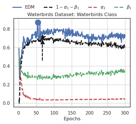
Figure 2: Euclidean Distance between Means (EDM) and noise parameters ($\alpha_{1},\beta_{1}$ and $1-\alpha_{1}-\beta_{1}$) for the positive target class of Waterbirds dataset. Blue dot indicates the model picked by Antigone, while black star indicates the model that maximizes $1-\alpha_{1}-\beta_{1}$.

Table 1: F1 scores and pseudo label accuracies (Ps. Acc.) We mark the best performance in bold. BM (blond men), BW (blond women), NBW (non-blond women) and NBM (non-blond men) for CelebA; WL (waterbirds landbkgd), WW (waterbirds waterbkgd), LW (landbirds waterbkgd) and LL (landbirds landbkgd) for Waterbirds.

	Antigone	GEORGE	GEORGE	Antigone
	(w/o EDM)		($k=2$)	(w/ EDM)
	CelebA (F1 Scores)
BM	0.28$\pm$ 0.01	0.13$\pm$ 0.02	0.12 $\pm$ 0.01	0.35$\pm$ 0.04
BW	0.95$\pm$ 0.01	0.43$\pm$ 0.04	0.51$\pm$ 0.02	0.96$\pm$ 0.00
NBW	0.22$\pm$ 0.02	0.42$\pm$ 0.01	0.6$\pm$ 0.01	0.22$\pm$ 0.01
NBM	0.67$\pm$ 0.01	0.4$\pm$ 0.02	0.31$\pm$ 0.01	0.68$\pm$ 0.01
Ps. Acc.	0.59$\pm$ 0.01	0.33$\pm$ 0.01	0.48$\pm$ 0.00	0.60$\pm$ 0.00
	Waterbirds (F1 Scores)
WL	0.41$\pm$ 0.02	0.43$\pm$ 0.02	0.52$\pm$ 0.01	0.76$\pm$ 0.03
WW	0.72$\pm$ 0.00	0.36$\pm$ 0.02	0.43$\pm$ 0.02	0.83$\pm$ 0.01
LW	0.58$\pm$ 0.02	0.44$\pm$ 0.03	0.55$\pm$ 0.03	0.78$\pm$ 0.04
LL	0.76$\pm$ 0.01	0.34$\pm$ 0.02	0.55$\pm$ 0.03	0.84$\pm$ 0.02
Ps. Acc.	0.68$\pm$ 0.01	0.30$\pm$ 0.02	0.53$\pm$ 0.03	0.81$\pm$ 0.02

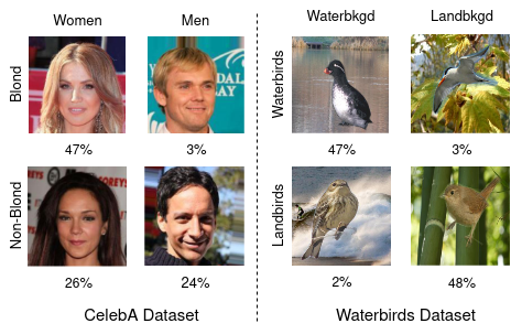
(a) Dataset Details

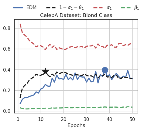
(b) EDM and noise parameters on Celeba

Figure 3: Figure (a) illustrates CelebA and Waterbirds datasets along with fraction of each sub-group examples in their respective training dataset. Figure (b) shows Euclidean Distance between Means (EDM) and noise parameters $\alpha_{1},\beta_{1}$ and and $1-\alpha_{1}-\beta_{1}$ for the positive target class of CelebA dataset. The noise parameters are unknown in practice. Blue dot indicates the model that we pick to generate pseudo sensitive attributes, while black star indicates the model that maximizes $1-\alpha_{1}-\beta_{1}$.

Quality of Antigone’s sensitive attribute labels: Antigone seeks to generate accurate sensitive attribute labels on validation data, referred to as pseudo label accuracy, based on the EDM criterion (Lemma 2.2). In Figure 2, we empirically validate Lemma 2.2 by plotting EDM and noise parameters $\alpha_{1}$ (contamination in majority group labels), $\beta_{1}$ (contamination in minority group labels) and $1-\alpha_{1}-\beta_{1}$ (proportionality constant between true and estimated fairness) on Waterbirds dataset (similar plot for CelebA dataset is in Appendix Figure 3(b)). From the figure, we observe that in both cases the EDM metric indeed captures the trend in $1-\alpha_{1}-\beta_{1}$, enabling early stopping at an epoch that minimizes contamination. The best early stopping points based on EDM and oracular knowledge of $1-\alpha_{1}-\beta_{1}$ are shown in a blue dot and star, respectively, and are very close.

Next, we evaluate the F1 scores of Antigone’s noisy sensitive attributes for all four subgroups in the CelebA and Waterbirds datasets. In  Table 1 we compare Antigone’s sensitive attribute labels’ F1 Score to GEORGE with the baseline number of clusters and GEORGE with $k=2$ clusters. Across CelebA and Waterbirds datasets and all four subgroups, we find that Antigone outperforms GEORGE except for one sub-group in CelebA dataset. Finally, Table 1 also reports results on a version of Antigone that uses standard ERM training instead of EDM (Antigone (w/o EDM)). We find that EDM provides higher pseudo-label accuracy compared to this baseline. Appendix Table 5 shows precision and recall of Antigone’s pseudo sensitive attribute labels and reaches the same conclusion.

Table 2: (Avg. target label accuracy, Fairness) on test data for different validation accuracy thresholds on the CelebA dataset. Lower DP and EO gaps are better. Higher WGA is better.

Val. Thresh.	Method	DP Gap	EO Gap	Worst-group Acc.
[94, 95)	Antigone $+$ JTT	(94.6, 15.0)$\pm$ (0.2, 0.7)	(94.7, 30.1)$\pm$ (0.2, 3.2)	(94.4, 59)$\pm$ (0.2, 4.7)
	Ground-Truth $+$ JTT	(94.7, 14.9)$\pm$ (0.2, 0.6)	(94.5, 30.4)$\pm$ (0.2, 2.3)	(94.3, 62.1)$\pm$ (0.3, 3.2)
[93, 94)	Antigone $+$ JTT	(93.7, 13.1)$\pm$ (0.2, 0.7)	(93.6, 26.4)$\pm$ (0.4, 5.0)	(93.4, 62.6)$\pm$ (0.2, 7.0)
	Ground-Truth $+$ JTT	(93.6, 13.1)$\pm$ (0.1, 0.6)	(93.6, 22.7)$\pm$ (0.3, 2.7)	(93.4, 67.9)$\pm$ (0.1, 1.9)
[92, 93)	Antigone $+$ JTT	(92.7, 11.1)$\pm$ (0.2, 0.5)	(92.3, 20.2)$\pm$ (0.2, 3.4)	(92.7, 68.1)$\pm$ (0.4, 3.7)
	Ground-Truth $+$ JTT	(92.7, 11.2)$\pm$ (0.3, 0.5)	(92.7, 16.9)$\pm$ (0.4, 2.9)	(92.7, 72.5)$\pm$ (0.2, 1.3)
[91, 92)	Antigone $+$ JTT	(91.7, 9.6)$\pm$ (0.1, 0.5)	(91.5, 16.3)$\pm$ (0.3, 3.4)	(91.3, 63.2)$\pm$ (0.3, 2.6)
	Ground-Truth $+$ JTT	(91.8, 9.7)$\pm$ (0.2, 0.5)	(91.8, 10.1)$\pm$ (0.3, 4.1)	(91.8, 77.3)$\pm$ (0.1, 2.4)
[90, 91)	Antigone $+$ JTT	(91.0, 8.3)$\pm$ (0.2, 0.4)	(90.9, 13.1)$\pm$ (0.1, 3.6)	(90.9, 63.1)$\pm$ (0.5, 4.4)
	Ground-Truth $+$ JTT	(91.0, 8.4)$\pm$ (0.2, 0.4)	(90.7, 6.8)$\pm$ (0.4, 3.7)	(91.4, 78.6)$\pm$ (0.2, 2.0)
	ERM	(95.8, 18.6)$\pm$ (0.0, 0.3)	(95.8, 46.4)$\pm$ (0.0, 2.2)	(95.8, 38.7)$\pm$ (0.0, 2.8)

Table 3: Performance of GEORGE using Antigone’s noisy validation data compared with GEORGE by itself. We observe that on CelebA and Waterbirds dataset, GEORGE $+$ Antigone out-performs GEORGE, even if GEORGE assumes knowledge of number of clusters $(k=2)$ in its clustering step. We show errors for over five runs.

	CelebA		Waterbirds
Method	Avg Acc	WGA	Avg Acc	WGA
ERM	95.7$\pm$0.1	34.5$\pm$3.1	95.9$\pm$0.2	29.7$\pm$1.6
GEORGE	93.6$\pm$0.3	60.4$\pm$2.3	95.5$\pm$0.7	50.0$\pm$5.8
Antigone + GEORGE	93.3$\pm$0.3	62.1$\pm$1.2	96.0$\pm$0.2	57.4$\pm$6.6
GEORGE (k=2)	94.6$\pm$0.1	62.6$\pm$2.1	95.0$\pm$0.8	46.7$\pm$11.7
Antigone +	94.2$\pm$0.3	65.3$\pm$2.9	95.8$\pm$0.6	54.4$\pm$7.1
GEORGE (k=2)

To understand the sensitivity of Antigone to minority group representation, we vary the fraction of minority group individuals from 5%, 20%, 35%, 50% in CelebA dataset. The results are shown in Appendix Table 6. As the dataset gets more balanced, the pseudo label accuracy reduces (as expected) because the trained models themselves become fairer. Nonetheless, the corresponding $1-\alpha-\beta$ values (also shown in the table) are unchanged till 20% of imbalance, and minority group individuals are over-represented in incorrect sets up to 35% imbalance.

Antigone+JTT: Next, in Table 2, we compare the test accuracy in predicting the target labels, quantified as target label accuracy, and fairness achieved by Antigone with JTT (Antigone+JTT) versus a baseline ERM model and with JTT using ground-truth sensitive attributes (Ground-Truth+JTT). As expected, baseline ERM yields unfair outcomes on all three fairness metrics: DP, EO and WGA. We observe that Antigone + JTT improves fairness over the baseline ERM model and closes the gap with Ground-Truth+JTT.

On both DP and EO, Antigone+JTT is very close to Ground-Truth+JTT in terms of both target label accuracy and fairness, and substantially improves on standard ERM models. On WGA, Antigone+JTT improves WGA from 38.7% for standard ERM to 68.1% at the expense of $3\%$ target label accuracy drop. Ground-Truth+JTT improves WGA further up to 78.6% but with a 4.4% target label accuracy drop. Data for Waterbirds (Appendix Table 7) and UCI Adults (Appendix Table 8) have the same trends.

Comparison with GEORGE: Like Antigone, GEORGE also generates pseudo-sensitive attributes on validation data, but as noted in Table 1, Antigone’s pseudo attribute labels are more accurate and have higher F1 scores than GEORGE’s. We now analyze how these improvements translate to greater fairness by comparing the WGA achieved by GEORGE alone versus Antigone+GEORGE in Table 3. On Waterbirds, Antigone+GEORGE has both 7.4% higher WGA and marginally higher target label accuracy than GEORGE. On Celeb-A, Antigone+GEORGE has 2.7% higher WGA but with a small 0.4% drop in target label accuracy. The results in  Table 3 are averaged over five runs, as is common in prior work. In interpreting the standard deviations, we note that the performance of Antigone+GEORGE and GEORGE are correlated over the five runs (likely because of a shared stage 2): for CelebA, Antigone+GEORGE’s WGA was equal to or better than GEORGE’s in each one of our five runs. Similarly, for Waterbirds, Antigone+GEORGE’s WGA is atleast 8.4% higher than GEORGE’s in each run, except in one run where GEORGE has 1% higher WGA.

Table 4: Antigone $+$ JTT vs Ideal MC $+$ JTT (Avg. target label accuracy, Fairness) comparison on test data for different validation accuracy thresholds on the CelebA dataset. Lower DP and EO gaps are better. Higher WGA is better.

		DP Gap	EO Gap	WGA
[94, 95)	Antigone $+$ JTT	(94.9, 14.7)	(94.6, 33.7)	(94.5, 61.7)
	Ideal MC $+$ JTT	(94.9, 14.7)	(94.4, 34.1)	(94.4, 58.3)
[93, 94)	Antigone $+$ JTT	(93.7, 12.2)	(93.9, 30.3)	(93.3, 60.0)
	Ideal MC $+$ JTT	(93.7, 12.2)	(93.5, 26.3)	(93.7, 65.0)
[92, 93)	Antigone $+$ JTT	(93.1, 12.1)	(92.4, 22.9)	(92.9, 65.6)
	Ideal MC $+$ JTT	(93.1, 12.1)	(93.0, 22.7)	(93.2, 69.4)
[91, 92)	Antigone $+$ JTT	(91.9, 9.3)	(91.1, 13.9)	(91.1, 66.7)
	Ideal MC $+$ JTT	(91.9, 9.3)	(92.2, 19.1)	(91.8, 73.9)
[90, 91)	Antigone $+$ JTT	(91.1, 7.9)	(91.1, 13.9)	(91.1, 66.7)
	Ideal MC $+$ JTT	(90.9, 8)	(90.4, 18.9)	(91.4, 72.2)

Ablation Studies:

We perform two ablation experiments to understand the benefits of Antigone’s proposed EDM metric. We already noted in Table 1 that Antigone with the proposed EDM metric produces higher quality sensitive attribute labels compared to a version of Antigone that picks hyper-parameters using standard ERM. We evaluated these two approaches using JTT’s training algorithm and find that Antigone with EDM results in a 5.7% increase in WGA and a small 0.06% increase in average target label accuracy

Second, in  Table 4, we also compare Antigone+JTT against a synthetically labeled validation dataset that exactly follows the ideal MC noise model in Section  2.3. We find that on DP Gap and EO Gap fairness metrics, Antigone ’s results are comparable (in fact sometimes slightly better) with those derived from the ideal MC model. On WGA, the most challenging fairness metric to optimize for, we find that the ideal MC model has a best-case WGA of 73.9% compared to Antigone’s 69.4%. This reflects the loss in fairness due to the gap between the assumptions of the idealized model versus Antigone’s implementation; however, the reduction in fairness is marginal when compared to the ERM baseline which has only a 38% WGA.

5 Related Work

Several works have observed that standard ERM training algorithms can achieve state-of-the-art accuracy on many tasks, but unintentionally make biased predictions for different sensitive attributes failing to meet the fairness objectives (Hovy & Søgaard, 2015; Oren et al., 2019; Hashimoto et al., 2018a; Buolamwini & Gebru, 2018).

Methods that seek to achieve fairness are of three types: pre-processing, in-processing and post-processing algorithms. Pre-processing (Quadrianto et al., 2019; Ryu et al., 2018) methods focus on curating the dataset that includes removal of sensitive information or balancing the datasets. In-processing methods (Hashimoto et al., 2018b; Agarwal et al., 2018; Zafar et al., 2019; Lahoti et al., 2020; Prost et al., 2019; Liu et al., 2021; Sohoni et al., 2020) alter the training mechanism by adding fairness constrains to the loss function or by training an adversarial framework to make predictions independent of sensitive attributes (Zhang et al., 2018). Post-processing methods (Hardt et al., 2016; Wang et al., 2020; Savani et al., 2020) alter the outputs, for e.g. use different threshold for different sensitive attributes. In this work, we focus on in-processing algorithms.

Prior in-processing algorithms, including the ones referenced above, assume access to sensitive attributes on the training data and validation dataset. Recent work sought to train fair model without training data annotations (Liu et al., 2021; Nam et al., 2020; Hashimoto et al., 2018a; Creager et al., 2021) but, except for GEORGE (Sohoni et al., 2020), require sensitive attributes on validation dataset to tune the hyperparameters. Like GEORGE, we seek to train fair classification models without ground-truth sensitive information on either training or validation dataset.

Antigone is different from GEORGE in three ways: (1) Unlike GEORGE, we account for the model prediction and the ground-truth target label to generate pseudo-sensitive attributes. (2) The hyper-parameters of the clustering step in GEORGE are fixed from literature and not specifically tuned for each dataset. In this paper, we propose a more principled approach to tune the model’s hyperparameters in an unsupervised fashion to obtain noisy sensitive features. And finally, (3) GEORGE only focuses on worst-group accuracy, whereas Antigone can be adapted to different notions of fairness.

A related body of work develops post-processing methods to improve fairness without access to sensitive attributes but assuming a small set of labelled data for auditing (Kim et al., 2019). One could use Antigone to create this auditing dataset, albeit with noise. Evaluating Antigone with these post-processing methods is an avenue for future work.

6 Conclusion

In this paper, we propose Antigone, a method to enable hyper-parameter tuning for fair ML models without access to sensitive attributes on training or validation sets. Antigone generates high-quality pseudo-sensitive attribute labels on validation data by training a family of biased classifiers using standard ERM and using correctly (incorrectly) classified examples as proxies for majority (minority) group membership. We propose a novel EDM metric based approach to pick the most biased model from this family and provide theoretical justification for this choice using the ideal MC noise model. The resulting validation dataset with pseudo sensitive attribute labels can then be used to tune the hyper-parameters of a fair training algorithm like JTT or GEORGE. We show that Antigone produces the highest quality of sensitive attributes compared to the state-of-art.

Appendix A Appendix

A.1 UCI Adult Dataset

Dataset details: Adult dataset (Dua & Graff, 2017) is used to predict if an individual’s annual income is $\leq 50K$ ($Y=0$) or $>50K$ ($Y=1$) based on several continuous and categorical attributes like the individual’s education level, age, gender, occupation, etc. The sensitive attribute is gender $A=\{\text{Men},\text{Women}\}$ (Zemel et al., 2013). The dataset consists of 45,000 instances and is split into training, validation and test sets with 21112, 9049 and 15060 instances, respectively. The dataset has twice as many men as women, and only $15\%$ of high income individuals are women. Consequently, the baseline ERM model under-performs on the minority group.

Hyper-parameter settings: In all our experiments using Adult dataset, we train a multi-layer neural network with one hidden layer consisting of 64 neurons. We train for a total of 100 epochs using the SGD optimizer and a batch size of 256. We tune Antigone and JTT by performing grid search over learning rates $\in\{1e-03,1e-04,1e-05\}$ and weight decays $\in\{1e-01,1e-03\}$. For JTT, we explore over $T\in\{1,2,5,10,15,20,30,35,40,45,50,65,80,95\}$ and $\lambda\in\{5,10,20\}$. In each case, we seek to optimize fairness while constraining average accuracy to ranges $\{[82,82.5),[81.5,82),[81,81.5),[80.5,81),[80,80.5)\}$.

A.2 Quality of Antigone’s Sensitive Attribute Labels

Table 5: We tabulate the precision, recall, F1-score of the noisy validation groups generated from ERM model, GEORGE, GEORGE with number of clusters $=2$ and Antigone. We observe that Antigone has higher precision and F1 scores across different noisy groups on CelebA and Waterbirds, respectively.

	Antigone	GEORGE	GEORGE	Antigone
	(w/o EDM)		($k=2$)	(w/ EDM)
	CelebA (Precision, Recall, F1 Scores)
Blond Men	0.26, 0.31, 0.28	0.09, 0.32, 0.13	0.06, 0.70, 0.12	0.36, 0.34, 0.35
	(0.02, 0.03, 0.01)	(0.01, 0.09, 0.02)	(0.01, 0.05, 0.01)	(0.05, 0.04, 0.04)
Blond Women	0.95, 0.94, 0.95	0.94, 0.28, 0.43	0.95, 0.35, 0.51	0.96, 0.96, 0.96
	(0.01, 0.01, 0.01)	(0.01, 0.04, 0.04)	(0.00, 0.02, 0.02)	(0.0, 0.0, 0.0)
Non-blond Women	0.82, 0.13, 0.22	0.51, 0.36, 0.42	0.5, 0.76, 0.6	0.86, 0.13, 0.22
	(0.01, 0.01, 0.02)	(0.00, 0.01, 0.01)	(0.00, 0.01, 0.01)	(0.01, 0.01, 0.01)
Non-blond Men	0.52, 0.97, 0.67	0.53, 0.33, 0.40	0.47, 0.23, 0.31	0.52, 0.98, 0.68
	(0.00, 0.00, 0.01)	(0.01, 0.02, 0.02)	(0.01, 0.01, 0.01)	(0.0, 0.0, 0.0)
CelebA Accuracy	0.59 $\pm$ 0.01	0.33 $\pm$ 0.01	0.48 $\pm$ 0.00	0.60 $\pm$ 0.00
	Waterbirds (Precision, Recall, F1 Scores)
Waterbirds Landbkgd	0.94, 0.26, 0.41	0.56, 0.34, 0.43	0.48, 0.57, 0.52	0.96, 0.63, 0.76
	(0.01, 0.02, 0.02)	(0.03, 0.02, 0.02)	(0.01, 0.01, 0.01)	(0.01, 0.04, 0.03)
Waterbirds Waterbkgd	0.57, 0.98, 0.72	0.55, 0.27, 0.36	0.48, 0.39, 0.43	0.73, 0.97, 0.83
	(0.01, 0.00, 0.00)	(0.07, 0.03, 0.02)	(0.02, 0.02, 0.02)	(0.02, 0.01, 0.01)
Landbirds Waterbkgd	0.96, 0.42, 0.58	0.57, 0.36, 0.44	0.55, 0.55, 0.55	0.97, 0.65, 0.78
	(0.00, 0.03, 0.02)	(0.04, 0.03, 0.03)	(0.03, 0.03, 0.03)	(0.00, 0.05, 0.04)
Landbirds Landbkgd	0.63, 0.98, 0.76	0.55, 0.24, 0.34	0.55, 0.56, 0.55	0.74, 0.98, 0.84
	(0.01, 0.00, 0.01)	(0.04, 0.04, 0.02)	(0.03, 0.04, 0.03)	(0.03, 0.00, 0.02)
Waterbirds Accuracy	0.68 $\pm$ 0.01	0.30 $\pm$ 0.02	0.53 $\pm$ 0.03	0.81 $\pm$ 0.02

Table 6: We tabulate the precision, recall, F1-score, pseudo label accuracy of the noisy validation groups generated by varying the fraction of minority group examples in each class of CelebA dataset. We observe that Antigone has higher precision, recall, F1 score and pseudo label accuracy if the imbalance is more in the training dataset.

Fraction Minority	5%	20%	35%	50%
	Precision, Recall, F1 Score
Blond Men (Minority)	0.57, 0.40, 0.47	0.81, 0.17, 0.29	0.67, 0.15, 0.24	0.75, 0.14, 0.24
Blond Women (Majority)	0.97, 0.98, 0.98	0.83, 0.99, 0.90	0.68, 0.96, 0.79	0.53, 0.95, 0.68
$1-\alpha_{1}-\beta_{1}$	0.54	0.64	0.35	0.28
Blond Ps. Acc	0.95	0.83	0.68	0.55
Non-blond Women (Minority)	0.45, 0.26, 0.33	0.59, 0.17, 0.26	0.63, 0.18, 0.28	0.63, 0.16, 0.26
Non-blond Men (Majority)	0.96, 0.98, 0.97	0.82, 0.97, 0.89	0.68, 0.94, 0.79	0.52, 0.91, 0.66
$1-\alpha_{0}-\beta_{0}$	0.41	0.41	0.31	0.15
Non-blond Ps. Acc.	0.94	0.81	0.67	0.54
Overall Ps. Acc.	0.95	0.81	0.67	0.54

A.3 Antigone + JTT

Table 7: We report the (Test average target label accuracy, Test fairness metric) for different validation accuracy thresholds on Waterbirds dataset. We observe that Antigone $+$ JTT (our noisy sensitive attributes) improves fairness over baseline ERM model and closes the gap with Ground-Truth $+$ JTT (ground-truth sensitive attributes).

Val. Thresh.	Method	DP Gap	EO Gap	Worst-group
[96, 96.5)	Antigone $+$ JTT	(95.8, 3.9) $\pm$ (0.4, 0.4)	(96.2, 10.7) $\pm$ (0.3, 7.1)	(96.3, 83.0) $\pm$ (0.4, 1.3)
	Ground-Truth $+$ JTT	(95.8, 3.9) $\pm$ (0.4, 0.4)	(96.0, 7.1) $\pm$ (0.3, 1.4)	(96.3, 83.0) $\pm$ (0.4, 1.3)
[95.5, 96)	Antigone $+$ JTT	(95.4, 2.8) $\pm$ (0.1, 0.1)	(96.0, 7.5) $\pm$ (0.2, 1.5)	(96.3, 83.2) $\pm$ (0.3, 0.6)
	Ground-Truth $+$ JTT	(95.4, 2.9) $\pm$ (0.4, 1.1)	(95.6, 6.0) $\pm$ (0.3, 2.1)	(96.1, 83.5) $\pm$ (0.5, 0.8)
[95, 95.5)	Antigone $+$ JTT	(94.5, 1.5) $\pm$ (0.6, 0.6)	(94.7, 4.2) $\pm$ (0.9, 3.1)	(94.7, 85.9) $\pm$ (0.9, 1.4)
	Ground-Truth $+$ JTT	(94.4, 1.7) $\pm$ (0.7, 0.7)	(94.3, 1.1) $\pm$ (0.5, 0.6)	(95.1, 86.8) $\pm$ (0.6, 1.1)
[94.5, 95)	Antigone $+$ JTT	(94.2, 0.4) $\pm$ (0.4, 0.4)	(93.8, 2.0) $\pm$ (0.5, 1.4)	(94.2, 86.7) $\pm$ (0.8, 1.8)
	Ground-Truth $+$ JTT	(93.6, 0.6) $\pm$ (0.5, 0.5)	(93.8, 2.0) $\pm$ (0.5, 1.4)	(94.1, 88.2) $\pm$ (0.6, 0.7)
[94.0, 94.5)	Antigone $+$ JTT	(93.0, 1.5) $\pm$ (0.6, 0.3)	(93.6, 4.8) $\pm$ (1.2, 3.0)	(93.7, 87.9) $\pm$ (0.5, 1.4)
	Ground-Truth $+$ JTT	(93.1, 1.5) $\pm$ (0.3, 0.4)	(93.2, 4.0) $\pm$ (1.0, 2.1)	(93.8, 88.1) $\pm$ (0.7, 1.1)
	ERM	(97.3, 21.3) $\pm$ (0.2, 1.1)	(97.3, 35.0) $\pm$ (0.2, 3.4)	(97.3, 59.1) $\pm$ (0.2, 3.8)

Table 8: (Avg. target label accuracy, Fairness) on test data for different validation accuracy thresholds on the UCI Adult dataset. Lower DP and EO gaps are better. Higher WGA is better.

Val. Thresh.	Method	DP Gap	EO Gap	Worst-group Acc.
[82, 82.5)	Antigone $+$ JTT	(81.9, 11.7)	(81.9, 0)	(81.7, 54.6)
	Ground-Truth $+$ JTT	(81.8, 11.9)	(81.4, 3.3)	(81.7, 54.6)
[81.5, 82)	Antigone $+$ JTT	(81.5, 9.3)	(81.5, 1.9)	(81.0, 56.0)
	Ground-Truth $+$ JTT	(81.5, 9.3)	(81.1, 4.0)	(81.0, 56.0)
[81, 81.5)	Antigone $+$ JTT	(80.8, 7.1)	(80.9, 0.9)	(81.0, 57.1)
	Ground-Truth $+$ JTT	(80.8, 7.1)	(81.0, 2.4)	(81.0, 57.1)
[80.5, 81)	Antigone $+$ JTT	(80.4, 7.2)	(80.1, 1.9)	(80.4, 58.2)
	Ground-Truth $+$ JTT	(79.8, 5.1)	(80.5, 5.0)	(80.5, 58.0)
[80, 80.5)	Antigone $+$ JTT	(79.7, 5.4)	(79.7, 1.4)	(80.4, 58.0)
	Ground-Truth $+$ JTT	(79.5, 3.9)	(80.4, 4.2)	(80.4, 58.0)
	ERM	(84.8, 53.8)	(84.8, 10.6)	(84.8, 52.4)

References

- Agarwal et al. (2018) Agarwal, A., Beygelzimer, A., Dudík, M., Langford, J., and Wallach, H. A reductions approach to fair classification, 2018.
- Bhatt et al. (2022) Bhatt, S., Dev, S., Talukdar, P., Dave, S., and Prabhakaran, V. Re-contextualizing fairness in nlp: The case of india, 2022. URL https://arxiv.org/abs/2209.12226.
- Buolamwini & Gebru (2018) Buolamwini, J. and Gebru, T. Gender shades: Intersectional accuracy disparities in commercial gender classification. In Friedler, S. A. and Wilson, C. (eds.), Proceedings of the 1st Conference on Fairness, Accountability and Transparency, volume 81 of Proceedings of Machine Learning Research, pp. 77–91. PMLR, 23–24 Feb 2018. URL https://proceedings.mlr.press/v81/buolamwini18a.html.
- Citron & Pasquale (2014) Citron, D. K. and Pasquale, F. The scored society: Due process for automated predictions. Wash. L. Rev., 89:1, 2014.
- Creager et al. (2021) Creager, E., Jacobsen, J.-H., and Zemel, R. Environment inference for invariant learning. In International Conference on Machine Learning, 2021.
- Dua & Graff (2017) Dua, D. and Graff, C. UCI machine learning repository, 2017. URL http://archive.ics.uci.edu/ml.
- Hardt et al. (2016) Hardt, M., Price, E., Price, E., and Srebro, N. Equality of opportunity in supervised learning. In Lee, D., Sugiyama, M., Luxburg, U., Guyon, I., and Garnett, R. (eds.), Advances in Neural Information Processing Systems, volume 29. Curran Associates, Inc., 2016. URL https://proceedings.neurips.cc/paper/2016/file/9d2682367c3935defcb1f9e247a97c0d-Paper.pdf.
- Hashimoto et al. (2018a) Hashimoto, T., Srivastava, M., Namkoong, H., and Liang, P. Fairness without demographics in repeated loss minimization. In International Conference on Machine Learning, pp. 1929–1938. PMLR, 2018a.
- Hashimoto et al. (2018b) Hashimoto, T. B., Srivastava, M., Namkoong, H., and Liang, P. Fairness without demographics in repeated loss minimization. In ICML, 2018b.
- Holstein et al. (2019) Holstein, K., Wortman Vaughan, J., Daumé, H., Dudik, M., and Wallach, H. Improving fairness in machine learning systems: What do industry practitioners need? In Proceedings of the 2019 CHI Conference on Human Factors in Computing Systems, CHI ’19, pp. 1–16, New York, NY, USA, 2019. Association for Computing Machinery. ISBN 9781450359702. doi: 10.1145/3290605.3300830. URL https://doi.org/10.1145/3290605.3300830.
- Hovy & Søgaard (2015) Hovy, D. and Søgaard, A. Tagging performance correlates with author age. In Proceedings of the 53rd Annual Meeting of the Association for Computational Linguistics and the 7th International Joint Conference on Natural Language Processing (Volume 2: Short Papers), pp. 483–488, Beijing, China, July 2015. Association for Computational Linguistics. doi: 10.3115/v1/P15-2079. URL https://aclanthology.org/P15-2079.
- Kim et al. (2019) Kim, M. P., Ghorbani, A., and Zou, J. Multiaccuracy: Black-box post-processing for fairness in classification. In Proceedings of the 2019 AAAI/ACM Conference on AI, Ethics, and Society, pp. 247–254, 2019.
- Lahoti et al. (2020) Lahoti, P., Beutel, A., Chen, J., Lee, K., Prost, F., Thain, N., Wang, X., and Chi, E. H. Fairness without demographics through adversarially reweighted learning, 2020.
- Lamy et al. (2019) Lamy, A., Zhong, Z., Menon, A. K., and Verma, N. Noise-Tolerant Fair Classification. Curran Associates Inc., Red Hook, NY, USA, 2019.
- Leslie (2020) Leslie, D. Understanding bias in facial recognition technologies. Technical report, 2020. URL https://zenodo.org/record/4050457.
- Liu et al. (2021) Liu, E. Z., Haghgoo, B., Chen, A. S., Raghunathan, A., Koh, P. W., Sagawa, S., Liang, P., and Finn, C. Just train twice: Improving group robustness without training group information. In Meila, M. and Zhang, T. (eds.), Proceedings of the 38th International Conference on Machine Learning, volume 139 of Proceedings of Machine Learning Research, pp. 6781–6792. PMLR, 18–24 Jul 2021. URL https://proceedings.mlr.press/v139/liu21f.html.
- Liu et al. (2015) Liu, Z., Luo, P., Wang, X., and Tang, X. Deep learning face attributes in the wild. In Proceedings of International Conference on Computer Vision (ICCV), December 2015.
- Markos et al. (2017) Markos, E., Milne, G. R., and Peltier, J. W. Information sensitivity and willingness to provide continua: A comparative privacy study of the united states and brazil. Journal of Public Policy & Marketing, 36(1):79–96, 2017. doi: 10.1509/jppm.15.159. URL https://doi.org/10.1509/jppm.15.159.
- Nam et al. (2020) Nam, J., Cha, H., Ahn, S., Lee, J., and Shin, J. Learning from failure: Training debiased classifier from biased classifier. In Advances in Neural Information Processing Systems, 2020.
- Oren et al. (2019) Oren, Y., Sagawa, S., Hashimoto, T. B., and Liang, P. Distributionally robust language modeling. In Proceedings of the 2019 Conference on Empirical Methods in Natural Language Processing and the 9th International Joint Conference on Natural Language Processing (EMNLP-IJCNLP), pp. 4227–4237, Hong Kong, China, November 2019. Association for Computational Linguistics. doi: 10.18653/v1/D19-1432. URL https://aclanthology.org/D19-1432.
- Pasquale (2015) Pasquale, F. The black box society: The secret algorithms that control money and information. Harvard University Press, 2015.
- Prost et al. (2019) Prost, F., Qian, H., Chen, Q., Chi, E. H., Chen, J., and Beutel, A. Toward a better trade-off between performance and fairness with kernel-based distribution matching, 2019.
- Quadrianto et al. (2019) Quadrianto, N., Sharmanska, V., and Thomas, O. Discovering fair representations in the data domain. In Proceedings of the IEEE/CVF Conference on Computer Vision and Pattern Recognition (CVPR), June 2019.
- Ryu et al. (2018) Ryu, H. J., Adam, H., and Mitchell, M. Inclusivefacenet: Improving face attribute detection with race and gender diversity, 2018.
- Sagawa* et al. (2020) Sagawa*, S., Koh*, P. W., Hashimoto, T. B., and Liang, P. Distributionally robust neural networks. In International Conference on Learning Representations, 2020. URL https://openreview.net/forum?id=ryxGuJrFvS.
- Savani et al. (2020) Savani, Y., White, C., and Govindarajulu, N. S. Intra-processing methods for debiasing neural networks, 2020.
- Scott et al. (2013) Scott, C., Blanchard, G., and Handy, G. Classification with asymmetric label noise: Consistency and maximal denoising. In Shalev-Shwartz, S. and Steinwart, I. (eds.), Proceedings of the 26th Annual Conference on Learning Theory, volume 30 of Proceedings of Machine Learning Research, pp. 489–511, Princeton, NJ, USA, 12–14 Jun 2013. PMLR. URL https://proceedings.mlr.press/v30/Scott13.html.
- Sohoni et al. (2020) Sohoni, N., Dunnmon, J., Angus, G., Gu, A., and Ré, C. No subclass left behind: Fine-grained robustness in coarse-grained classification problems. In Larochelle, H., Ranzato, M., Hadsell, R., Balcan, M., and Lin, H. (eds.), Advances in Neural Information Processing Systems, volume 33, pp. 19339–19352. Curran Associates, Inc., 2020. URL https://proceedings.neurips.cc/paper/2020/file/e0688d13958a19e087e123148555e4b4-Paper.pdf.
- Veale & Binns (2017) Veale, M. and Binns, R. Fairer machine learning in the real world: Mitigating discrimination without collecting sensitive data. Big Data & Society, 4(2):2053951717743530, 2017. doi: 10.1177/2053951717743530. URL https://doi.org/10.1177/2053951717743530.
- Wang et al. (2020) Wang, Z., Qinami, K., Karakozis, I. C., Genova, K., Nair, P., Hata, K., and Russakovsky, O. Towards fairness in visual recognition: Effective strategies for bias mitigation, 2020.
- Zafar et al. (2019) Zafar, M. B., Valera, I., Gomez-Rodriguez, M., and Gummadi, K. P. Fairness constraints: A flexible approach for fair classification. Journal of Machine Learning Research, 20(75):1–42, 2019. URL http://jmlr.org/papers/v20/18-262.html.
- Zemel et al. (2013) Zemel, R., Wu, Y., Swersky, K., Pitassi, T., and Dwork, C. Learning fair representations. In International conference on machine learning, pp. 325–333. PMLR, 2013.
- Zhang et al. (2018) Zhang, B. H., Lemoine, B., and Mitchell, M. Mitigating unwanted biases with adversarial learning, 2018.