P3H-23-008, TTP23-004, TU-1178, ZU-TH 06/23
Analytic approximations of $2\to 2$ processes with massive internal particles

Abstract

We consider two-loop corrections to $2\to 2$ scattering processes with massive particles in the final state and massive particles in the loop. We discuss the combination of analytic expansions in the high-energy limit and for small Mandelstam variable $t$. For the example of double Higgs boson production we show that the whole phase space can be covered and time-consuming numerical integrations can be avoided.

1 Introduction

In many higher-order calculations of cross sections the virtual corrections are the bottleneck, particularly if they involve massive particles propagating in loops. A prominent example of such a process is Higgs boson pair production, where the real-radiation contribution with exact dependence on the top quark mass [2] was available long before the corresponding virtual corrections [3, 4, 5]. One of the reasons is certainly the enormous expressions which are present in intermediate stages of the calculation, and the complicated integrals which in general depend on several invariants. Often a purely numerical approach for the evaluation of the loop integrals is necessary, which comes with the well-known disadvantages of long run-times and reduced flexibility in the choice of values for parameters. In this paper we suggest an alternative approach for the computation of virtual loop integrals for $2\to 2$ processes. It is based on the combination expansions in different kinematic regions.

We consider the scattering of two (massless) partons in the initial state with momenta $q_{1}$ and $q_{2}$ into two massive particles in the final state with momenta $q_{3}$ and $q_{4}$. It is convenient to introduce the Mandelstam variables as

$$s=(q_{1}+q_{2})^{2}\,,\qquad t=(q_{1}+q_{3})^{2}\,,\qquad u=(q_{1}+q_{4})^{2}\,,$$ (1)

where all momenta are incoming. Furthermore we have

$$q_{1}^{2}=q_{2}^{2}=0\,,\qquad q_{3}^{2}=m_{X}^{2}\,,\qquad q_{4}^{2}=m_{Y}^{2}\,,$$ (2)

where in general $m_{X}$ and $m_{Y}$ are allowed to be different and the transverse momentum of the final-state particles is given by

$$p_{T}^{2} = \frac{u\,t-m_{X}^{2}m_{Y}^{2}}{s}\,.$$ (3)

For definiteness we will denote the internal mass by $m_{t}$, the top quark mass.

The computation of massive two-loop integrals with the kinematics described above is a difficult problem. Purely numerical approaches have been developed and applied to the processes $gg\to HH$, $gg\to ZZ$, $gg\to ZH$, $gg\to W^{+}W^{-}$ (see, e.g., Refs. [3, 4, 5, 6, 7, 8]). Usually these computations require a large amount of CPU time for a single phase space point. Furthermore, it is often necessary to fix numerical values for the top quark and Higgs boson masses at an early stage of the calculation. Thus a change of value or renormalization scheme makes it necessary to repeat a large part of the calculation.

In order to avoid the disadvantages of a purely numerical calculation a number of analytic approximation methods have been developed. Initially they have usually been applied to Higgs boson pair production and afterwards also to more complicated processes. Among the approximations for $gg\to HH$ are large top quark mass expansions [9, 10, 11], high-energy expansions [12, 13], small transverse-momentum expansions [14] and expansions around the top quark threshold [15]. In Refs. [16, 17] a method has been developed where the two-loop amplitude is expanded for small Higgs boson mass with a subsequent numerical evaluation.

Since such approximations are only valid in a restricted phase space it is tempting to combine different approaches. A first example of such a combination has been presented in Ref. [18] where the exact numerical results from Refs. [3, 4] were combined with the high-energy expansion of Refs. [12, 13]. The CPU-time expensive calculations were only necessary for relatively small values of the Higgs transverse momentum, say below $p_{T}\approx 200$ GeV, and the fast evaluation of the analytic high-energy expansions could be used for the remaining phase space.

A similar approach to the one proposed in this paper has been discussed in Refs. [19, 20] where the analytic small $p_{T}$ and high-energy expansions are “merged”. For both expansions Padé approximations are constructed, however, only to low order ($[1/1]$ and $[6/6]$, respectively). The Padé approximants are constructed from the analytic expression and kept fixed, thus there is no estimation of the uncertainty due to this approach. In our approach high-order Padé approximants are constructed numerically in the high-energy region and the approach of Ref. [21] is used to determine an uncertainty estimate. Furthermore, instead of an expansion in $p_{T}$ we perform an expansion in the Mandelstam variable $t$. We believe that our approach leads to simpler expressions in intermediate steps. Note that in [19, 20] only terms up to $m_{H}^{2}$ have been used in the high-energy approximation. This introduces a systematic uncertainty of up to a few percent, as we will discuss below. In this work we will include quartic corrections which reduces this uncertainty below the percent level.

In this paper we review the high-energy expansion method developed in Refs. [13, 18, 21]. An improvement in the method allows us to obtain significantly deeper expansions in $m_{t}^{2}/s$, $m_{t}^{2}/t$ and $m_{t}^{2}/u$ which includes terms up to about $m_{t}^{120}$ (see also Ref. [22]) (instead of $m_{t}^{32}$ as in [13, 21]). The deeper expansions combined with the construction of Padé approximants extends the range of validity to even smaller values of $\sqrt{s}$ and $p_{T}$. We will provide details regarding this approach in Section 2.1.

In Section 2.2 we will describe our approach for the expansion around $t\to 0$. It is based on the observation that for this limit a simple Taylor expansion can be performed, rather than a complicated asymptotic expansion. We can thus reduce the calculation to integrals which only depend on $m_{t}^{2}/s$. These integrals are obtained with the help of differential equations using the “expand and match” approach developed in Refs. [23, 24]. The boundary conditions are obtained from the large-$m_{t}$ limit, in which the integrals are simple and can be computed analytically.

In Section 3 we will use the process $gg\to HH$ to illustrate the methods of Sections 2.1 and 2.2. However, the approach is more general and with straightforward modifications it can also be applied to other processes as, e.g., $gg\to ZH$. We will show that we can cover the whole kinematic phase space which we parametrize in terms of $\sqrt{s}$ and $p_{T}$. A summary of our findings together with a discussion of possible bottlenecks are discussed in Section 4.

2 Analytic expansions

We begin by performing a Taylor expansion in the masses of the final-state particles. This is always possible for diagrams where the final-state particles couple to massive internal lines. This produces an amplitude in terms of four-point functions which depend on $s$, $t$ and $m_{t}$, but not on $m_{X}$ or $m_{Y}$. We then proceed by considering analytic expansions of the amplitude in the following limits:

• high energy

• $t\to 0$

In both cases we perform an exact reduction of the amplitude to master integrals, which we then expand in the relevant limit. The reduction is the same for both cases, leading to the same master integrals. For the process $gg\to HH$ this step was first done in Refs. [12, 13] and leads to 161 two-loop master integrals. In the following subsections we briefly discuss the features of methods A and B in more detail.

It is also possible to perform an asymptotic expansion in the limit of a large top quark mass. In this case it is not necessary to expand in the masses of the final state particles. Such an expansion is automated in the program exp [25, 26] and the approach is well established; results for the $gg\to HH$ form factors at three loops can be found in Refs. [10, 27]. In this work we use the results of this approach to provide boundary conditions for the differential equations considered in method B described above. We also show some numerical values for the form factors in this approximation in Section 3.3, however our proposed procedure to approximate the two-loop form factors requires only the high-energy and small-$t$ expansions.

2.1 High-energy expansion

The method of high-energy expansion, including a subsequent Padé approximant–based improvement, has been developed in Ref. [12, 13, 18, 21, 28]. We improve this approach by constructing a deeper expansion of the master integrals, which includes 120 terms in the small-$m_{t}$ expansion. Such an expansion is obtained in the following way:

1. We insert an ansatz for the expansion of each master integral $M_{i}$, $i=1,...,161$

   $$M_{i}(\epsilon,s,t,m_{t}) = \sum\limits_{a=-3}^{a_{i,\text{max}}}\sum\limits_{b=-3}^{b_{\text{max}}}\sum\limits_{c=0}^{4+a}c_{abc}^{(i)}(s,t)\>\epsilon^{a}\>\left(\frac{m_{t}}{\sqrt{s}}\right)^{b}\>\ln\left(\frac{m_{t}^{2}}{s}\right)^{c}~{},$$ (4)

   into the system of differential equations for the master integrals, with respect to $m_{t}$. $a_{i,\text{max}}$ is a master integral–specific value determined by the $\epsilon$ order required to produce the amplitude to $\epsilon^{0}$ and we choose $b_{\text{max}}=120$ for each master integral. The planar master integrals depend only on even powers of $m_{t}$, while the non-planar integrals also have contributions from odd powers as was shown in Ref. [13].

2. By comparing the coefficients of powers of $\epsilon$, $m_{t}$ and $\ln(m_{t})$ we establish a system of linear equations for the expansion coefficients $c_{abc}^{(i)}(s,t)$, which depend on the Mandelstam variables $s$ and $t$. We solve this system in terms of a small number of boundary constants by making use of the reduce_user_defined_system feature of Kira [29]. Solving over finite fields with subsequent rational reconstruction using FireFly [30, 31] is much faster than solving symbolically using Fermat [32]. It is this method of solving the system of equations which allows us to expand much more deeply than Ref. [13], which expands only up to $b_{\text{max}}=32$.

3. The boundary constants can be fixed using the solutions from Refs. [12, 13], where these constants were computed using the method of regions and Mellin-Barnes techniques, see also Ref. [33] for more details.

The expansion coefficients of the master integrals are then exported to a FORM Tablebase which is used to efficiently insert the expansions into the amplitude, which is also expanded in $\epsilon$ and $m_{t}$ to the required depth.

The subsequent Padé approximation is performed numerically following Refs. [18, 21]. For convenience we repeat the important steps in the following. The starting point is a form factor as an expansion in $m_{t}$, i.e., numerical values for all other kinematic variables and masses are inserted. We then apply the replacements $m_{t}^{2k}\to m_{t}^{2k}x^{k}$ and $m_{t}^{2k-1}\to m_{t}^{2k-1}x^{k}$ to pair together the even and odd powers of $m_{t}$, yielding a degree-$N$ polynomial in the variable $x$, with half the maximum degree of the $m_{t}$ expansion.

Next we construct Padé approximants in the variable $x$ and write the form factor as a rational function of the form

$$[n/m](x) = \frac{a_{0}+a_{1}x+\ldots+a_{n}x^{n}}{1+b_{1}x+\ldots+b_{m}x^{m}}\,,$$ (5)

where the coefficients $a_{i}$ and $b_{i}$ are determined by comparing the coefficients of $x^{k}$ after expanding the right-hand side of Eq. (5) around the point $x=0$. Evaluation of this rational function at $x=1$ yields the Padé approximated value for the form factor.

The numerator and denominator degrees $(n,m)$ in Eq. (5) are free parameters; one only must ensure that $n+m\leq N$ such that a sufficient number of expansion terms are available to determine the coefficients $a_{i}$ and $b_{i}$. We define $N_{\rm low}$ and $N_{\rm high}$ and include Padé approximations in our analysis which fulfil

$$N_{\rm low}\leq n+m\leq N_{\rm high}\quad\textnormal{and}\quad N_{\rm low}\leq n+m-|n-m|\,.$$ (6)

Our default choice is $N_{\rm low}=49$ and $N_{\rm high}=56$ which leads to 28 different Padé approximants. They are combined using three different criteria:

• The rational function in Eq. (5) develops poles at the roots of the denominator. We give more weight to those Padé approximants which have poles further away from the evaluation point $x=1$ (“pole-distance re-weighted” Padé approximation).

• We give more weight to Padé approximants which are derived from a larger number of expansion terms.

• We give more weight to “near-diagonal” Padé approximants.

We combine the weights from each criterion for each of the Padé approximants, and use the combined weight to produce a central value and corresponding uncertainty for the phase-space point under consideration. Explicit formulae for the individual steps of the construction are given in Section 4 of Ref. [21]. In the supplementary material [34] to this paper we provide Mathematica code which can be used to construct, for a given polynomial in $x$, an approximation based on the procedure described above, including an uncertainty estimate.

We have demonstrated this approach applied to a single planar master integral in Ref. [22] and the comparison to (exact) numerical results can be found in Fig. 7(a) of that reference. In Fig. LABEL:fig::non-pl_MI we discuss results for the non-planar integral shown in Fig. 1. We choose $p_{T}=40$ GeV and vary $\sqrt{s}$ between 300 GeV and 1100 GeV. In Fig. LABEL:fig::non-pl_MI(a) we compare Padé results constructed from expansions up to $m_{t}^{32}$ and $m_{t}^{112}$, which are shown by the green and orange bands, respectively. One observes a dramatic reduction of the uncertainty. At the same time it is reassuring to see that the uncertainty estimate of the Padé procedure is reliable, when comparing to the numerical values obtained using FIESTA [35]. In Fig. LABEL:fig::non-pl_MI(b) we focus on the comparison of the orange band with the results from FIESTA; we observe good agreement within uncertainties in the whole plotted range of $\sqrt{s}$, even very close to the threshold for the production of two top quarks.

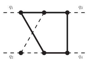
Figure 1: The two-loop Feynman diagram $G_{59}(1,1,1,1,1,1,1,-1,0)$ (see Appendix A of Ref. [13] for more details). Solid and dashed lines correspond to massive and massless propagators. All external momenta are massless.

2.2 Expansion for $t\to 0$

In this subsection we aim for an expansion of the original 161 master integrals around $t=0$ such that the amplitude can be expanded in this limit. This complements the the high-energy expansion, i.e. we aim for a good description in the region around the threshold where $s\approx 4m_{t}^{2}$ and the high-energy expansion breaks down. However, as we will see below, good results are also obtained for larger values of $\sqrt{s}$, in particular for smaller values of $p_{T}$. The expansion is performed as follows.

• As for the high-energy expansion, we first expand in the masses of the final-state particles. For $gg\to HH$ it is sufficient to expand up to $m_{H}^{4}$ to obtain a precision below the percent level. We are left with integral families which depend on $s,t$ and $m_{t}$. Here we note that the expansion in $m_{H}$ generates spurious $1/t$ terms which cancel after inserting the $t$-expansion of the master integrals.

  As discussed previously, this expansion is a simple Taylor expansion in cases where the final-state particles couple to massive internal lines; otherwise, a more involved asymptotic expansion must be performed.

• Establish differential equations, with respect to $t$, for the master integrals of the $2\to 2$ problem where all external lines are massless. The master integrals, and thus the resulting $t$-differential equations, are the same as in the high-energy case discussed in Section 2.1.

• We use the differential equations to obtain, for each master integral, a generic Taylor expansion around $t=0$. This is achieved by expanding the coefficients of the differential equations around $t\to 0$ and for each master integral, inserting an ansatz of the form

  $$M_{i}(\epsilon,s,t,m_{t}) = \sum_{a=-3}^{a_{i,\text{max}}}\sum_{b\geq 0}c_{ab}^{(i)}(s,m_{t}^{2})\>\epsilon^{a}\>\left(\frac{t}{m_{t}^{2}}\right)^{b}\,,$$

  where the (unknown) coefficients $c_{ab}^{(i)}(s,m_{t}^{2})$ are functions of $s$ and $m_{t}^{2}$.

Note that for $t\to 0$ some of the propagators of the original integral families (see Appendix A of Refs. [12] and [13]) become linearly dependent. After a partial fraction decomposition we can define new integral families which contain fewer propagators. In terms of these new families, the number of master integrals in the $t\to 0$ limit reduces from 161 to 48. One of the resulting topologies has been studied in Ref. [36], where it was shown that two master integrals are elliptic and cannot be expressed in terms of iterated integrals. These master integrals depend on two different square roots.

We have calculated all 46 non-elliptic master integrals analytically by solving the associated differential equations in the variable $s/m_{t}^{2}$ following the algorithms outlined in Ref. [37] implemented with the help of the packages Sigma [38], OreSys [39] and HarmonicSums [40]. The boundary conditions have been fixed in the large-$m_{t}$ limit, where the integrals can be calculated by performing a large mass expansion, implemented in q2e/exp [25, 26]. Our final result can be expressed in terms of iterated integrals over letters which contain the three square roots $\sqrt{x}\sqrt{4-x},\sqrt{x}\sqrt{4+x},\sqrt{4-x}\sqrt{4+x}$. However, we find that this representation is not well suited for numerical evaluation for several reasons:

1. Some of the iterated integrals depend on two square-root valued letters at the same time, which cannot easily be rationalized simultaneously.

2. The iterated integrals have spurious poles at $s/m_{t}^{2}=1$ and $s/m_{t}^{2}=4$, which require analytic continuation.

3. The analytic results for the two elliptic integrals are rather involved.

Therefore, we calculate all 48 master integrals using the semi-analytic approach developed in Refs. [41, 42]. For each master integral, we provide a deep expansion of 50 terms around different values of $s/m_{t}^{2}$, with high-precision numerical coefficients. In particular we construct expansions around 18 values of $s/m_{t}^{2}$ to cover values of $s$ between 0 and $\infty$. Our starting point for the construction of the approximations is the expansion around $s=0$ where all master integrals can be computed analytically. As a by-product we extend the large-$m_{t}$ expansion of these master integrals (but only at $t=0$).

This method has a number of advantages compared to purely numerical approaches. Since the value of $m_{t}$ is only inserted into the final expression, it is possible to easily change the value or renormalization scheme used for $m_{t}$. It is straightforward to take derivatives w.r.t. $m_{t}$ of the one-loop expressions in order to generate the corresponding counterterm contributions.

3 Application to Higgs boson pair production

In this section we apply the expansion methods discussed above to the particular case of the $gg\to HH$ amplitude. We start by examining the $m_{H}$ and $t$ expansions of one-loop master integrals by comparing to numerical results obtained with FIESTA [35] and Package-X [43]. We show that the Taylor expansion in $m_{H}$ produces good agreement with the exact result, even for smaller values of $\sqrt{s}$ close to the Higgs pair production threshold at $\sqrt{s}=2m_{H}$. Afterwards we discuss results for the one- and two-loop form factors. Finally we compare the virtual corrections to the Higgs pair production cross section with the numerical results obtained in Ref. [18].

For the numerical evaluations we use input values for the top quark and Higgs boson masses of $m_{t}=173.21$ GeV and $m_{H}=125.1$ GeV, respectively.

For completeness we provide in the following the definition of the form factors for Higgs boson pair production. The amplitude for the process $g(q_{1})g(q_{2})\to H(q_{3})H(q_{4})$ can be decomposed into two Lorentz structures ($a$ and $b$ are adjoint colour indices)

$${\cal M}^{ab} = \varepsilon_{1,\mu}\varepsilon_{2,\nu}{\cal M}^{\mu\nu,ab}\,\,=\,\,\varepsilon_{1,\mu}\varepsilon_{2,\nu}\delta^{ab}X_{0}s\left(F_{1}A_{1}^{\mu\nu}+F_{2}A_{2}^{\mu\nu}\right)\,,$$ (7)

where

$$A_{1}^{\mu\nu} = g^{\mu\nu}-{\frac{1}{q_{12}}q_{1}^{\nu}q_{2}^{\mu}}\,,$$

$$A_{2}^{\mu\nu} = g^{\mu\nu}+\frac{1}{{p_{T}^{2}}q_{12}}\left(q_{33}q_{1}^{\nu}q_{2}^{\mu}-2q_{23}q_{1}^{\nu}q_{3}^{\mu}-2q_{13}q_{3}^{\nu}q_{2}^{\mu}+2q_{12}q_{3}^{\mu}q_{3}^{\nu}\right)\,.$$ (8)

Here we have introduced the abbreviation $q_{ij}=q_{i}\cdot q_{j}$ and $p_{T}$ is given in Eq. (3). The prefactor $X_{0}$ is given by

$$X_{0} = \frac{G_{F}}{\sqrt{2}}\frac{\alpha_{s}(\mu)}{2\pi}T_{F}\,,$$ (9)

where $T_{F}=1/2$, $G_{F}$ is Fermi’s constant and $\alpha_{s}(\mu)$ is the strong coupling constant evaluated at the renormalization scale $\mu$.

We define the expansion in $\alpha_{s}$ of the form factors as

$$F = F^{(0)}+\frac{\alpha_{s}(\mu)}{\pi}F^{(1)}+\cdots\,,$$ (10)

and decompose the functions $F_{1}$ and $F_{2}$ introduced in Eq. (7) into “triangle” and “box” form factors. We thus cast the one- and two-loop corrections in the form ($k=0,1$)

$$F_{1}^{(k)} = \frac{3m_{H}^{2}}{s-m_{H}^{2}}F^{(k)}_{\rm tri}+F^{(k)}_{\rm box1}+\delta_{k1}F^{(1)}_{\rm dt1}\,,$$

$$F_{2}^{(k)} = F^{(k)}_{\rm box2}+\delta_{k1}F^{(1)}_{\rm dt2}\,.$$ (11)

$F^{(1)}_{\rm dt1}$ and $F^{(1)}_{\rm dt2}$ denote the contribution from one-particle reducible double-triangle diagrams, see, e.g. Fig. 1(f) of Ref. [18]. The main focus in this paper is on $F^{(1)}_{\rm box1}$ and $F^{(1)}_{\rm box2}$. Analytic results for the leading-order form factors are available from [44, 45] and the two-loop triangle form factors have been computed in Refs. [46, 47, 48]. The results for the double-triangle contribution can be found in [11].

3.1 Expansion of a one-loop master integral in $m_{H}$

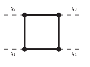
Figure 3: The one-loop master integral $G_{2}(1,1,1,1)$, where all internal lines are massive and for the external lines we have $q_{1}^{2}=q_{2}^{2}=0$ and $q_{3}^{2}=q_{4}^{2}=m_{H}^{2}$.

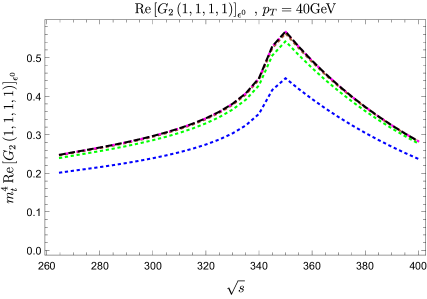
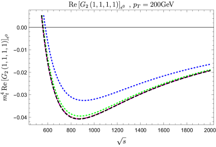
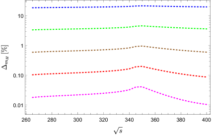
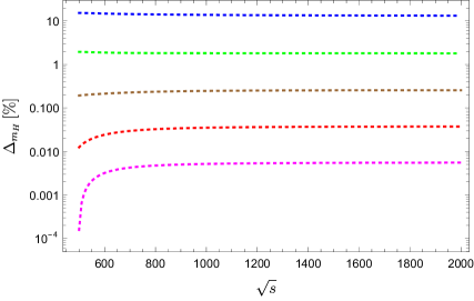
Figure 4: Real part of the master integral $G_{2}(1,1,1,1)$ as a function of $\sqrt{s}$ for $p_{T}=40$ GeV (left) and $p_{T}=200$ GeV (right). The coloured lines include expansions in $m_{H}$ up to the indicated orders. The exact result is shown in black. The lower panels show the relative error between the expansions and the exact curve.

In Fig. 4 we show, as a function of $\sqrt{s}$, the real part of the one-loop box master integral $G_{2}(1,1,1,1)$ (see Appendix A of Ref. [12] for details on the notation), which is depicted in Fig. 3. The left and right panels correspond to $p_{T}=40$ GeV and $p_{T}=200$ GeV, respectively. The coloured lines show expansions in $m_{H}^{2}$ up to fourth order, and the black line represents the exact result. After the Taylor expansion in $m_{H}$ a reduction to master integrals is necessary. It has been performed with LiteRed [49] and for the numerical evaluation of the resulting master integrals we have used Package-X [43].

The upper row shows the results for the master integral and the lower row shows the relative error between the expansions and the exact curve. One observes that the $m_{H}^{0}$ curves do not describe the exact result particularly well, with differences at the 15-20% level, however including the quadratic and quartic terms provide a description below the 5% level and 1% level, respectively; these observations are largely independent of the values of $\sqrt{s}$ and $p_{T}$.

3.2 Expansion of a one-loop master integral in $t$

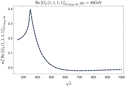
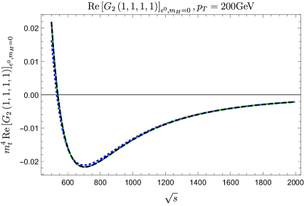
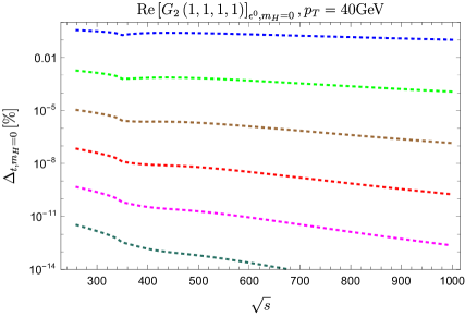
Figure 5: Real part of the master integral $G_{2}(1,1,1,1)$ as a function of $\sqrt{s}$ for $p_{T}=40$ GeV (left) and $p_{T}=200$ GeV (right). The coloured lines include expansions in $t$ up to $t^{10}$. The exact result is shown in black. The lower panels show the relative error between the expansions and the exact curve.

Next we study the $t\to 0$ expansion of the same one-loop box master integral, $G_{2}(1,1,1,1)$. For this purpose we choose $m_{H}=0$, i.e., the leading term of the expansion discussed in Section 3.1. We perform the expansion in $t$ using LiteRed [49] and then map the resulting integrals to new integral families which have only three propagators and depend only on $s/m_{t}^{2}$. For these integrals we establish a system of differential equations which can be solved analytically, incorporating boundary conditions from the $s\to 0$ limit. The resulting coefficients of the polynomial in $t$ can be written in terms of Harmonic Polylogarithms [50], which we evaluate using the Mathematica package HPL.m [51, 52].

In Fig. 5 we show the convergence of the $t$ expansion for the values $p_{T}=40$ GeV and $p_{T}=200$ GeV in the left and right columns, respectively. The lower row shows the relative error between the expansion and the exact curve. For the smaller value of $p_{T}=40$ GeV, we observe that the leading expansion term ($t^{0}$) already reproduces the exact result at the percent level. For $p_{T}=200$ GeV the leading term does not perform so well, however by including higher-order terms the expansion converges on the exact result very quickly.

3.3 Expansion of the one-loop form factors

We now discuss the high-energy and small-$t$ expansions at the level of the one-loop form factors $F_{\rm box1}^{(0)}$ and $F_{\rm box2}^{(0)}$, and compare them to the exact results.

In Figs. 6 and 7 we show, for various values of $p_{T}$, the results for the form factors $F_{\rm box1}^{(0)}$ and $F_{\rm box2}^{(0)}$ as a function of $\sqrt{s}$. The high-energy and small-$t$ expansions are shown as coloured dashed lines; the solid black line (in the background) corresponds to the exact result. For these plots we have incorporated quartic expansion terms in $m_{H}$, the order which is also available at the two-loop level. Furthermore, for the small-$t$ expansion terms up to $t^{5}$ are taken into account and the high-energy expansion includes Padé approximations which include terms up to at least $(m_{t}^{2})^{49}$ and at most $(m_{t}^{2})^{56}$.

Above the top quark pair threshold we observe that both expansions agree with the exact result even for values of $p_{T}$ as small as $50$ GeV and as large as $200$ GeV. For larger values of $p_{T}$ the small-$t$ expansion starts to deviate from the black curve, as can be seen in the panel for $p_{T}=300$ GeV, whereas the high-energy approximation agrees very well, as expected. On the other hand, for values of $p_{T}$ below $50$ GeV the small-$t$ expansion provides an excellent approximation. From the panels in Figs. 6 and 7 one observes that for $100~{}\mbox{GeV}\lesssim p_{T}\lesssim 200$ GeV both approximations work well for $\sqrt{s}\gtrsim 350$ GeV.

Below the top quark pair threshold we observe that the small-$t$ expansion provides an excellent description of the exact result, whereas the high-energy expansion deviates; this is expected since it does not contain any information about the threshold. Values $\sqrt{s}\lesssim 2m_{t}$ are kinematically only allowed for $p_{T}\lesssim 120$ GeV.

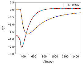
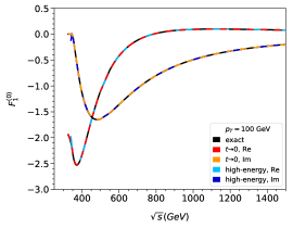
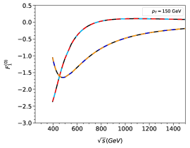
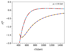
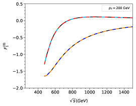
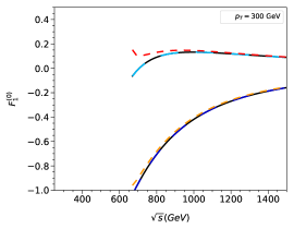
Figure 6: One-loop form factor $F_{\rm box1}^{(0)}$ as a function of $\sqrt{s}$ for various values of $p_{T}$.

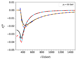
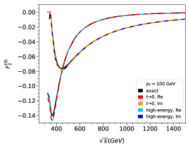
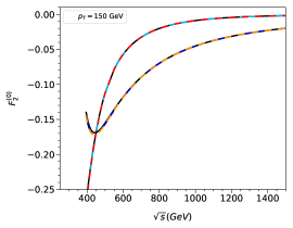
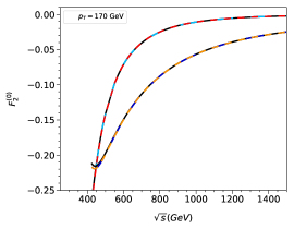
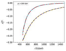
Figure 7: One-loop form factor $F_{\rm box2}^{(0)}$ as a function of $\sqrt{s}$ for various values of $p_{T}$.

To quantify the quality of the approximations we show in Tabs. 1, 2 and 3, for three different values of $p_{T}$, results for the real part of $F_{\rm box1}^{(0)}$ for various values of $\sqrt{s}$. We show the exact results, the results for the small-$t$ expansion for different expansion depths in $m_{H}$, the high-energy expansion including terms up to $m_{H}^{4}$, and results for the large-$m_{t}$ expansion (LME) up to $1/m_{t}^{12}$ [27].

Let us start the discussion with Tab. 1 ($p_{T}=50$ GeV) where we observe the following:

• If we restrict ourselves to the approximation which includes quartic $m_{H}$ terms, in the region above the top quark threshold we observe an agreement of at least 3 significant digits between the small-$t$ and high-energy expansions.

• The agreement between the exact result and the approximations based on an expansion in $m_{H}$ up to quartic order is well below the percent level.

• Including expansion terms in $m_{H}$, beyond the quartic terms, for the small-$t$ expansion improves the agreement with the exact result.

Similar conclusions also hold for $p_{T}=200$ GeV, as can be seen in Tab. 2. In practical applications the high-energy expansion can be used for such values of $p_{T}$.

The purpose of Tab. 3 is to show that the small-$t$ expansion also works for small values of $p_{T}$ and large values of $\sqrt{s}$. It is impressive that for such small values of $p_{T}$ the high-energy expansion still provides good approximations for $\sqrt{s}$ values around $400$ GeV. This demonstrates the power of a deep expansion in $m_{t}$ combined with a Padé improvement. For larger values of $\sqrt{s}$ the high-energy expansion breaks down, because it is no longer the case that $|t|\gg m_{t}^{2}$.

For $F_{\rm box2}^{(0)}$ the comparison is not so straightforward, as can be seen in the first two panels of Fig. 7 and in Tab. 4. We observe that the expansion in $m_{H}$ does not converge sufficiently quickly for the quartic terms to provide a good description of the exact curve for $p_{T}\lesssim 100$ GeV. While including terms to $m_{H}^{8}$ in the small-$t$ expansion again provides good agreement, such expansion terms are not available at two loops.

We show in Tab. 4 that below the top quark pair production threshold, the large top quark expansion of Ref. [27] (including expansion terms to $1/m_{t}^{12}$) provides a good approximation of the exact result and can be used instead in this region. However, $F_{\rm box2}^{(0)}$ is numerically much smaller than $F_{\rm box1}^{(0)}$; we have verified that the use of the large top quark expansion in this region does not affect the results and conclusions of Section 3.5.

$\sqrt{s}$ (GeV)		$270$	$300$	$350$	$400$	$610$	$990$
exact		$-1.72013$	$-1.81435$	$-2.32246$	$-2.34773$	$-0.393996$	$0.0855054$
small-$t$	$m_{H}^{0}$	$-1.44108$	$-1.52523$	$-1.92423$	$-2.01154$	$-0.420989$	$0.0626770$
	$m_{H}^{2}$	$-1.67642$	$-1.77026$	$-2.25482$	$-2.30931$	$-0.404100$	$0.0837986$
	$m_{H}^{4}$	$-1.71321$	$-1.80759$	$-2.31050$	$-2.34518$	$-0.395265$	$0.0854682$
	$m_{H}^{6}$	$-1.71902$	$-1.81331$	$-2.32026$	$-2.34808$	$-0.394063$	$0.0855094$
	$m_{H}^{8}$	$-1.71995$	$-1.81419$	$-2.32204$	$-2.34793$	$-0.393990$	$0.0855057$
high-en.	$m_{H}^{4}$	—	—	$-2.31129$	$-2.34521$	$-0.395262$	$0.0854694$
LME		$-1.71813$	$-1.80468$	$-2.08865$	$-2.76874$	—	—

Table 1: Real part of $F_{\rm box1}^{(0)}$ for $p_{T}=50$ GeV.

$\sqrt{s}$ (GeV)		$610$	$990$
exact		$-0.311182$	$0.110469$
small-$t$	$m_{H}^{0}$	$-0.340443$	$0.089788$
	$m_{H}^{2}$	$-0.319571$	$0.109173$
	$m_{H}^{4}$	$-0.311692$	$0.110538$
	$m_{H}^{6}$	$-0.310705$	$0.110570$
	$m_{H}^{8}$	$-0.310651$	$0.110567$
high-energy	$m_{H}^{4}$	$-0.312218$	$0.110440$

Table 2: Real part of $F_{\rm box1}^{(0)}$ for $p_{T}=200$ GeV.

$\sqrt{s}$ (GeV)		$270$	$300$	$350$	$400$	$610$	$990$
exact		$-1.72358$	$-1.81816$	$-2.32666$	$-2.35282$	$-0.400246$	$0.0835134$
small-$t$	$m_{H}^{0}$	$-1.44780$	$-1.52956$	$-1.92815$	$-2.01570$	$-0.426920$	$0.0605334$
	$m_{H}^{2}$	$-1.68133$	$-1.77444$	$-2.25910$	$-2.31430$	$-0.410425$	$0.0817808$
	$m_{H}^{4}$	$-1.71707$	$-1.81151$	$-2.31474$	$-2.35027$	$-0.401533$	$0.0834753$
	$m_{H}^{6}$	$-1.72257$	$-1.81714$	$-2.32446$	$-2.35317$	$-0.400314$	$0.0835175$
	$m_{H}^{8}$	$-1.72342$	$-1.81800$	$-2.32624$	$-2.35302$	$-0.400239$	$0.0835137$
high-en.	$m_{H}^{4}$	—	—	$-2.32046$	$-2.35382$	$-0.464921$	$-0.539285$
LME		$-1.72158$	$-1.80854$	$-2.09373$	$-2.77895$	—	—

Table 3: Real part of $F_{\rm box1}^{(0)}$ for $p_{T}=10$ GeV.

From the considerations above, we propose the following selection criteria for the choice of expansion in the different regions of the $\{\sqrt{s},p_{T}\}$ plane:

• Below $p_{T}=150$ GeV: use small-$t$ expansion for all values of $\sqrt{s}$.

• For $150$ GeV$\lesssim p_{T}\lesssim 200$ GeV either approximation can be used.

• Above $p_{T}=200$ GeV use the high-energy expansion for all values of $\sqrt{s}$.

As a consequence, below $\sqrt{s}=2m_{t}$ the small-$t$ expansion is always selected. The fact that the high-energy and small-$t$ expansions agree with each other (and with the exact result) in the region $150$ GeV$\lesssim p_{T}\lesssim 200$ GeV increases our confidence in the accuracy of the expansions; we will check for this agreement at two loops, where no exact analytic result for the form factors is available.

$\sqrt{s}$ (GeV)		$270$	$300$	$350$	$400$	$610$	$990$
exact		$-0.025050$	$-0.026046$	$-0.033323$	$-0.029569$	$-0.006633$	$-0.001207$
small-$t$	$m_{H}^{0}$	$-0.111991$	$-0.072393$	$-0.064400$	$-0.050849$	$-0.009550$	$-0.001571$
	$m_{H}^{2}$	$-0.069277$	$-0.058082$	$-0.061193$	$-0.048812$	$-0.008496$	$-0.001339$
	$m_{H}^{4}$	$-0.033254$	$-0.031982$	$-0.039319$	$-0.032503$	$-0.006558$	$-0.001190$
	$m_{H}^{6}$	$-0.026450$	$-0.027041$	$-0.034525$	$-0.029807$	$-0.006603$	$-0.001206$
	$m_{H}^{8}$	$-0.025286$	$-0.026208$	$-0.033565$	$-0.029543$	$-0.006631$	$-0.001207$
high-en.	$m_{H}^{4}$	—	—	$-0.039369$	$-0.032504$	$-0.006558$	$-0.001189$
LME		$-0.024977$	$-0.025767$	$-0.028531$	$-0.034309$	—	—

Table 4: Real part of $F_{\rm box2}^{(0)}$ for $p_{T}=50$ GeV.

3.4 Two-loop form factors

In the following we present results for the two-loop box form factors where for the ultra-violet renormalization and infra-red subtraction we follow Ref. [13]. In particular, we renormalize the top quark mass in the on-shell scheme.

In Figs. 8, 9, 10 and 11 we show the results for the two colour factors of the two-loop form factors, for various values of $p_{T}$, as a function of $\sqrt{s}$. For the small-$t$ expansion terms up to $t^{5}$ are taken into account and the high-energy expansion includes Padé approximations with at least $(m_{t}^{2})^{49}$ and at most $(m_{t}^{2})^{56}$ terms. In all cases quartic terms in $m_{H}$ are included. Results for the high-energy form factors at the deeper expansion depths considered here are provided in the ancillary files of this paper [34].

An exact result for the form factors is not at our disposal, however, we observe that the approximations show a very similar behaviour as at one-loop order. In particular, we observe that for $100$ GeV$\lesssim p_{T}\lesssim 200$ GeV there is a wide range in $\sqrt{s}$ where we find excellent agreement between the two approximations. We want to stress that for these $p_{T}$ values the small-$t$ expansion works well even for larger values of $\sqrt{s}$. This is demonstrated by the black and gray curves which show the relative percentage difference between the small-$t$ and high-energy expansions for the real and imaginary parts of the form factors, respectively. For each value of $100$ GeV$\lesssim p_{T}\lesssim 170$ GeV there is an overlap region in which the relative difference is far below 1%, and mostly even below $0.1\%$. Note that the spikes in the gray and black curves are related to zeros of the form factors.

For $p_{T}>200$ GeV we can rely on the high-energy expansion. This is supported by the fact that even for $p_{T}\approx 100$ GeV the high-energy expansion agrees with the small-$t$ expansion even for $\sqrt{s}\approx 2m_{t}$. Note that for $\sqrt{s}<2m_{t}$ the high-energy expansion is not valid for any value of $p_{T}$ since no information about the top quark pair threshold is used for the construction of the approximation. However, for $\sqrt{s}<2m_{t}$ the small-$t$ approximation is always valid since $p_{T}$ is kinematically constrained to be less than about 120 GeV.

For smaller values of $p_{T}$ the small-$t$ expansion is even more reliable, as can been seen from the one-loop comparison in Tab. 3.

In summary, in Sections 2.1 and 2.2 we demonstrate that the combination of the small-$t$ and high-energy expansions is sufficient to cover the whole phase space, and that the final uncertainty is given only by the expansion in $m_{H}$ which we estimate to be below 1%.

In our current implementation in Mathematica we have an explicit dependence on all parameters ($m_{t},m_{H},s$ and $t$) which allows for a straightforward change of parameter values or renormalization scheme. Thus the computing time required to evaluate the form factors is not very optimized. Nevertheless, it takes just a few seconds to evaluate the small $t$ expansion. The numerical evaluation of the high-energy expansion and the subsequent Padé approximation takes between 40 and 50 seconds. If required a significant speed-up is possible.

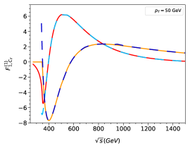
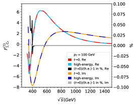
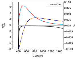
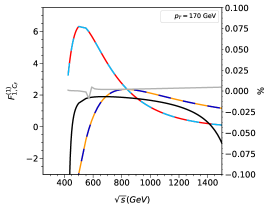
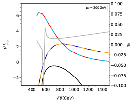
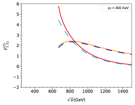
Figure 8: $C_{F}$ contribution to the two-loop form factor $F_{\rm box1}^{(1)}$ as a function of $\sqrt{s}$ for various values of $p_{T}$.

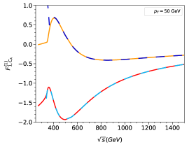
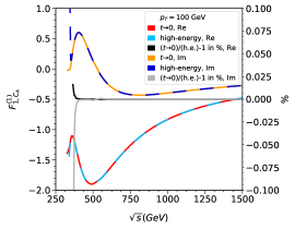
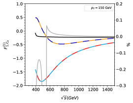
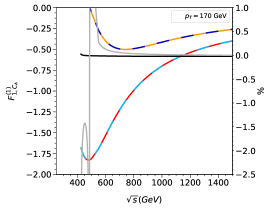
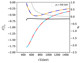
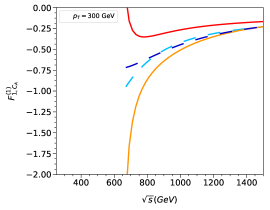
Figure 9: $C_{A}$ contribution to the two-loop form factor $F_{\rm box1}^{(1)}$ as a function of $\sqrt{s}$ for various values of $p_{T}$.

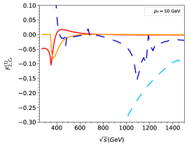
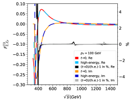
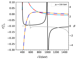
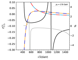
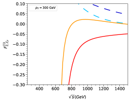
Figure 10: $C_{F}$ contribution to the two-loop form factor $F_{\rm box2}^{(1)}$ as a function of $\sqrt{s}$ for various values of $p_{T}$.

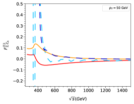
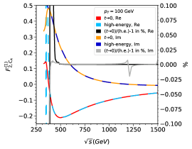
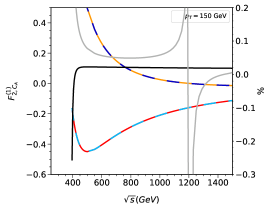
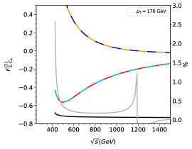
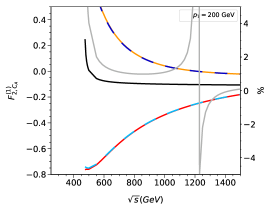
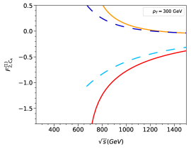
Figure 11: $C_{A}$ contribution to the two-loop form factor $F_{\rm box2}^{(1)}$ as a function of $\sqrt{s}$ for various values of $p_{T}$.

3.5 Virtual NLO corrections

As a final comparison, we construct the infra-red subtracted virtual corrections, following Ref. [53]. They are given by

$$\widetilde{\mathcal{V}}_{\textnormal{fin}} = \frac{\alpha_{s}^{2}\left(\mu\right)}{16\pi^{2}}\frac{G_{F}^{2}s^{2}}{64}\left[C+2\left({\tilde{F}_{1}^{(0)*}}\tilde{F}_{1}^{(1)}+{\tilde{F}_{2}^{(0)*}}\tilde{F}_{2}^{(1)}+\tilde{F}_{1}^{(0)}{\tilde{F}_{1}^{(1)*}}+\tilde{F}_{2}^{(0)}{\tilde{F}_{2}^{(1)*}}\right)\right]\,,$$ (12)

with

$$C = \left[\left|\tilde{F}_{1}^{(0)}\right|^{2}+\left|\tilde{F}_{2}^{(0)}\right|^{2}\right]\left(C_{A}\pi^{2}-C_{A}\log^{2}\frac{\mu^{2}}{s}\right)\,,$$ (13)

where $\alpha_{s}$ corresponds to the five-flavour strong coupling constant. It is convenient to introduce the $\alpha_{s}$-independent quantity

$$\mathcal{V}_{\textnormal{fin}} = \frac{\widetilde{\mathcal{V}}_{\textnormal{fin}}}{\alpha_{s}^{2}(\mu)}\,.$$ (14)

We use the exact expressions for the one-loop form factors along with the approximations discussed in the previous section for the two-loop form factors, to compute $\mathcal{V}_{\textnormal{fin}}$. The triangle and double-triangle diagrams are included in the form factors, as described in Eq. (11); we use exact expressions for the double-triangle diagrams, while for the triangle diagrams we use the expansions discussed above.

In Ref. [18] the high-energy expansions of Refs. [12, 13, 33] have been combined with the exact, numerical two-loop results of [53], such that $\mathcal{V}_{\textnormal{fin}}$ can be evaluated at any phase-space point and costly two-loop numerical integrations are only required in a restricted phase space, namely for $p_{T}<150$ GeV if $\sqrt{s}\geq 700$ GeV and for $p_{T}<200$ GeV if $\sqrt{s}<700$ GeV. The results of [18] are collected as data points in hhgrid [54]. The high-energy expansion used in [18] only includes terms up to $m_{t}^{32}$, in contrast to the much deeper expansions which we consider in this work.

Figure 12: ${\cal V}_{\rm fin}$ as a function of $p_{T}$, normalized to the central values of the pySecDec-evaluated points of hhgrid. We switch from the small-$t$ to the high-energy expansion at $p_{T}=175$ GeV.

In Fig. 12 we compare our new results for $\mathcal{V}_{\textnormal{fin}}$ to those obtained using pySecDec [55, 56] in Ref. [18]. The grey data points and uncertainties correspond to the pySecDec data points, normalized to their central values. In comparison the uncertainty of our approximation is negligible. The blue and red data points are obtained from the small-$t$ and high-energy expansions, where we normalize to the central values of the hhgrid data. This plot may be compared with Fig. 3 of Ref. [18].

To quantify the agreement between our approximations and the pySecDec evaluations, the following table describes the proportion of points which are contained within a number of pySecDec error intervals.
pySecDec err. intervals 1$\sigma$ 2$\sigma$ 3$\sigma$ small-$t$ 0.57 0.85 0.92 high-energy 0.65 0.94 0.99
We observe that the high-energy expansion demonstrates a Gaussian behaviour, while the small-$t$ expansion shows a non-Gaussian disagreement, which we ascribe to the systematic error due to the slower convergence of the $m_{H}^{2}$ expansion in the lower-$p_{T}$ region, as shown in Fig. 4.

Let us finally compare to the findings of Refs. [19, 20]. In these works the integration over $t$ has been performed and an uncertainty of $1\%$ is claimed. We present detailed results for the form factors and find a several-digit agreement in the overlap region for $p_{T}\approx 100$ GeV to $200$ GeV. On the other hand, the result for the form factors in Refs. [19, 20] suggest a several-percent difference between the expansions in some cases.

In Refs. [19, 20] only 13 high-energy terms have been taken into account to construct a $[6/6]$ Padé approximant and thus the transition from the small-$p_{T}$ to the high-energy approximation is made at relatively high values of $p_{T}$ ($p_{T}\approx 312$ GeV and $340$ GeV for the choices $\sqrt{s}=900$ GeV and $\sqrt{s}=2000$ GeV in Fig. 3 of Ref. [19]). As we show in Figs. 6 and 7 the $t\to 0$ expansion does not perform very well in this region. In our approach, we use the high-energy expansion at much smaller values of $p_{T}$ so this region is well described. Let us also mention that in Refs. [19, 20] only quadratic $m_{H}$ terms are taken into account which leads to a few-percent systematic uncertainty at the level of the form factors.

In the small-$p_{T}$ expansion in Refs. [19, 20] only a $[1/1]$ Padé approximant is constructed which means that three expansion terms are available. In our analysis we use terms up to $t^{5}$, i.e. six expansion terms; no Padé improvement of the $t\to 0$ expansion is necessary.

4 Conclusions

In this paper we consider a $2\to 2$ process with massive internal particles, which is a multi-scale problem and thus notoriously difficult, both in an analytic and in a numerical approach. We show that the combination of analytic expansions in two regions of phase space provides a complete description of the two-loop virtual amplitude. On the one hand we consider a deep expansion in the high-energy limit where the internal mass (in our application, the top quark mass) is small compared to the Mandelstam variables $s$ and $t$. On the other hand we perform an expansion in $t$ which again eliminates a scale from the integrand. In both cases we expand in the mass of the final-state particles.

We discuss in detail the two-loop corrections for $gg\to HH$ and show that for this process no numerical integration is necessary to obtain the differential virtual corrections. Other processes such as $gg\to ZH$ or $gg\to ZZ$ can be treated in analogy.

Using a similar approach to the one developed in this paper it might be possible to extend the $t\to 0$ expansion to three loops, yielding the NNLO virtual corrections to this gluon fusion processes. Possible bottlenecks, which have to be studied in the future, are huge intermediate expressions and the integration-by-parts reduction of the expanded amplitudes to master integrals.

References

- [1]
- [2] F. Maltoni, E. Vryonidou and M. Zaro, JHEP 11 (2014), 079 [arXiv:1408.6542 [hep-ph]].
- [3] S. Borowka, N. Greiner, G. Heinrich, S. P. Jones, M. Kerner, J. Schlenk, U. Schubert and T. Zirke, Phys. Rev. Lett. 117 (2016) no.1, 012001 [erratum: Phys. Rev. Lett. 117 (2016) no.7, 079901] [arXiv:1604.06447 [hep-ph]].
- [4] S. Borowka, N. Greiner, G. Heinrich, S. P. Jones, M. Kerner, J. Schlenk and T. Zirke, JHEP 10 (2016), 107 [arXiv:1608.04798 [hep-ph]].
- [5] J. Baglio, F. Campanario, S. Glaus, M. Mühlleitner, M. Spira and J. Streicher, Eur. Phys. J. C 79 (2019) no.6, 459 [arXiv:1811.05692 [hep-ph]].
- [6] B. Agarwal, S. P. Jones and A. von Manteuffel, JHEP 05 (2021), 256 [arXiv:2011.15113 [hep-ph]].
- [7] L. Chen, G. Heinrich, S. P. Jones, M. Kerner, J. Klappert and J. Schlenk, JHEP 03 (2021), 125 doi:10.1007/JHEP03(2021)125 [arXiv:2011.12325 [hep-ph]].
- [8] C. Brønnum-Hansen and C. Y. Wang, JHEP 05 (2021), 244 [arXiv:2101.12095 [hep-ph]].
- [9] S. Dawson, S. Dittmaier and M. Spira, Phys. Rev. D 58 (1998), 115012 [arXiv:hep-ph/9805244 [hep-ph]].
- [10] J. Grigo, J. Hoff, K. Melnikov and M. Steinhauser, Nucl. Phys. B 875 (2013), 1-17 doi:10.1016/j.nuclphysb.2013.06.024 [arXiv:1305.7340 [hep-ph]].
- [11] G. Degrassi, P. P. Giardino and R. Gröber, Eur. Phys. J. C 76 (2016) no.7, 411 [arXiv:1603.00385 [hep-ph]].
- [12] J. Davies, G. Mishima, M. Steinhauser and D. Wellmann, JHEP 03 (2018), 048 doi:10.1007/JHEP03(2018)048 [arXiv:1801.09696 [hep-ph]].
- [13] J. Davies, G. Mishima, M. Steinhauser and D. Wellmann, JHEP 01 (2019), 176 doi:10.1007/JHEP01(2019)176 [arXiv:1811.05489 [hep-ph]].
- [14] R. Bonciani, G. Degrassi, P. P. Giardino and R. Gröber, Phys. Rev. Lett. 121 (2018) no.16, 162003 [arXiv:1806.11564 [hep-ph]].
- [15] R. Gröber, A. Maier and T. Rauh, JHEP 03 (2018), 020 [arXiv:1709.07799 [hep-ph]].
- [16] X. Xu and L. L. Yang, JHEP 01 (2019), 211 [arXiv:1810.12002 [hep-ph]].
- [17] G. Wang, Y. Wang, X. Xu, Y. Xu and L. L. Yang, Phys. Rev. D 104 (2021) no.5, L051901 [arXiv:2010.15649 [hep-ph]].
- [18] J. Davies, G. Heinrich, S. P. Jones, M. Kerner, G. Mishima, M. Steinhauser and D. Wellmann, JHEP 11 (2019), 024 doi:10.1007/JHEP11(2019)024 [arXiv:1907.06408 [hep-ph]].
- [19] L. Bellafronte, G. Degrassi, P. P. Giardino, R. Gröber and M. Vitti, JHEP 07 (2022), 069 doi:10.1007/JHEP07(2022)069 [arXiv:2202.12157 [hep-ph]].
- [20] G. Degrassi, R. Gröber, M. Vitti and X. Zhao, JHEP 08 (2022), 009 doi:10.1007/JHEP08(2022)009 [arXiv:2205.02769 [hep-ph]].
- [21] J. Davies, G. Mishima, M. Steinhauser and D. Wellmann, JHEP 04 (2020), 024 doi:10.1007/JHEP04(2020)024 [arXiv:2002.05558 [hep-ph]].
- [22] J. Davies, G. Mishima, K. Schönwald, M. Steinhauser and H. Zhang, JHEP 08 (2022), 259 doi:10.1007/JHEP08(2022)259 [arXiv:2207.02587 [hep-ph]].
- [23] M. Fael, F. Lange, K. Schönwald and M. Steinhauser, SciPost Phys. Proc. 7 (2022), 041 [arXiv:2110.03699 [hep-ph]].
- [24] M. Fael, F. Lange, K. Schönwald and M. Steinhauser, Phys. Rev. D 106 (2022) no.3, 034029 [arXiv:2207.00027 [hep-ph]].
- [25] T. Seidensticker, hep-ph/9905298.
- [26] R. Harlander, T. Seidensticker and M. Steinhauser, Phys. Lett. B 426 (1998) 125 [hep-ph/9712228].
- [27] J. Davies and M. Steinhauser, JHEP 10 (2019), 166 doi:10.1007/JHEP10(2019)166 [arXiv:1909.01361 [hep-ph]].
- [28] J. Davies, G. Mishima and M. Steinhauser, JHEP 03 (2021), 034 doi:10.1007/JHEP03(2021)034 [arXiv:2011.12314 [hep-ph]].
- [29] J. Klappert, F. Lange, P. Maierhöfer and J. Usovitsch, Comput. Phys. Commun. 266 (2021), 108024 [arXiv:2008.06494 [hep-ph]].
- [30] J. Klappert, S. Y. Klein and F. Lange, Comput. Phys. Commun. 264 (2021), 107968 [arXiv:2004.01463 [cs.MS]].
- [31] J. Klappert and F. Lange, Comput. Phys. Commun. 247 (2020), 106951 [arXiv:1904.00009 [cs.SC]].
- [32] R. H. Lewis, Fermat’s User Guide, http://www.bway.net/~lewis.
- [33] G. Mishima, JHEP 02 (2019), 080 [arXiv:1812.04373 [hep-ph]].
-
[34]
https://www.ttp.kit.edu/preprints/2023/ttp23-004/. - [35] A. V. Smirnov, N. D. Shapurov and L. I. Vysotsky, Comput. Phys. Commun. 277 (2022), 108386 [arXiv:2110.11660 [hep-ph]].
- [36] A. von Manteuffel and L. Tancredi, JHEP 06 (2017), 127 [arXiv:1701.05905 [hep-ph]].
- [37] J. Ablinger, J. Blümlein, P. Marquard, N. Rana and C. Schneider, Nucl. Phys. B 939 (2019), 253-291 [arXiv:1810.12261 [hep-ph]].
- [38] C. Schneider, Sém. Lothar. Combin. 56 (2007) 1, article B56b; C. Schneider, in: Computer Algebra in Quantum Field Theory: Integration, Summation and Special Functions Texts and Monographs in Symbolic Computation eds. C. Schneider and J. Blümlein (Springer, Wien, 2013) 325 arXiv:1304.4134 [cs.SC].
- [39] S. Gerhold, Uncoupling systems of linear Ore operator equations, Diploma Thesis, RISC, J. Kepler University, Linz, 2002.
- [40] J. A. M. Vermaseren, Int. J. Mod. Phys. A 14 (1999), 2037-2076 [arXiv:hep-ph/9806280 [hep-ph]]; J. Blümlein, Comput. Phys. Commun. 180 (2009), 2218-2249 [arXiv:0901.3106 [hep-ph]]; J. Ablinger, Diploma Thesis, J. Kepler University Linz, 2009, arXiv:1011.1176 [math-ph]; J. Ablinger, J. Blümlein and C. Schneider, J. Math. Phys. 52 (2011) 102301 [arXiv:1105.6063 [math-ph]]; J. Ablinger, J. Blümlein and C. Schneider, J. Math. Phys. 54 (2013), 082301 [arXiv:1302.0378 [math-ph]]; J. Ablinger, Ph.D. Thesis, J. Kepler University Linz, 2012, arXiv:1305.0687 [math-ph]; J. Ablinger, J. Blümlein and C. Schneider, J. Phys. Conf. Ser. 523 (2014), 012060 [arXiv:1310.5645 [math-ph]]; J. Ablinger, J. Blümlein, C. G. Raab and C. Schneider, J. Math. Phys. 55 (2014), 112301 [arXiv:1407.1822 [hep-th]]; J. Ablinger, PoS LL2014 (2014), 019 [arXiv:1407.6180 [cs.SC]]; J. Ablinger, [arXiv:1606.02845 [cs.SC]]; J. Ablinger, PoS RADCOR2017 (2017), 069 [arXiv:1801.01039 [cs.SC]]; J. Ablinger, PoS LL2018 (2018), 063; J. Ablinger, [arXiv:1902.11001 [math.CO]].
- [41] M. Fael, F. Lange, K. Schönwald and M. Steinhauser, JHEP 09 (2021), 152 doi:10.1007/JHEP09(2021)152 [arXiv:2106.05296 [hep-ph]].
- [42] M. Fael, F. Lange, K. Schönwald and M. Steinhauser, Phys. Rev. Lett. 128 (2022) no.17, 172003 doi:10.1103/PhysRevLett.128.172003 [arXiv:2202.05276 [hep-ph]].
- [43] H. H. Patel, Comput. Phys. Commun. 218 (2017) 66 [arXiv:1612.00009 [hep-ph]].
- [44] E. W. N. Glover and J. J. van der Bij, Nucl. Phys. B 309 (1988), 282-294
- [45] T. Plehn, M. Spira and P. M. Zerwas, Nucl. Phys. B 479 (1996), 46-64 [erratum: Nucl. Phys. B 531 (1998), 655-655] [arXiv:hep-ph/9603205 [hep-ph]].
- [46] R. Harlander and P. Kant, JHEP 12 (2005), 015 [arXiv:hep-ph/0509189 [hep-ph]].
- [47] C. Anastasiou, S. Beerli, S. Bucherer, A. Daleo and Z. Kunszt, JHEP 01 (2007), 082 [arXiv:hep-ph/0611236 [hep-ph]].
- [48] U. Aglietti, R. Bonciani, G. Degrassi and A. Vicini, JHEP 01 (2007), 021 [arXiv:hep-ph/0611266 [hep-ph]].
- [49] R. N. Lee, J. Phys. Conf. Ser. 523 (2014), 012059 [arXiv:1310.1145 [hep-ph]].
- [50] E. Remiddi and J. A. M. Vermaseren, Int. J. Mod. Phys. A 15 (2000), 725-754 [arXiv:hep-ph/9905237 [hep-ph]].
- [51] D. Maitre, Comput. Phys. Commun. 174 (2006), 222-240 [arXiv:hep-ph/0507152 [hep-ph]].
- [52] D. Maitre, Comput. Phys. Commun. 183 (2012), 846 [arXiv:hep-ph/0703052 [hep-ph]].
- [53] G. Heinrich, S. P. Jones, M. Kerner, G. Luisoni and E. Vryonidou, JHEP 08 (2017), 088 [arXiv:1703.09252 [hep-ph]].
-
[54]
https://github.com/mppmu/hhgrid. - [55] S. Borowka, G. Heinrich, S. Jahn, S. P. Jones, M. Kerner, J. Schlenk and T. Zirke, Comput. Phys. Commun. 222 (2018), 313-326 [arXiv:1703.09692 [hep-ph]].
- [56] S. Borowka, G. Heinrich, S. Jahn, S. P. Jones, M. Kerner and J. Schlenk, Comput. Phys. Commun. 240 (2019), 120-137 [arXiv:1811.11720 [physics.comp-ph]].