Lower Bounds for Learning in Revealing POMDPs

Abstract

This paper studies the fundamental limits of reinforcement learning (RL) in the challenging partially observable setting. While it is well-established that learning in Partially Observable Markov Decision Processes (POMDPs) requires exponentially many samples in the worst case, a surge of recent work shows that polynomial sample complexities are achievable under the revealing condition—A natural condition that requires the observables to reveal some information about the unobserved latent states. However, the fundamental limits for learning in revealing POMDPs are much less understood, with existing lower bounds being rather preliminary and having substantial gaps from the current best upper bounds.

We establish strong PAC and regret lower bounds for learning in revealing POMDPs. Our lower bounds scale polynomially in all relevant problem parameters in a multiplicative fashion, and achieve significantly smaller gaps against the current best upper bounds, providing a solid starting point for future studies. In particular, for multi-step revealing POMDPs, we show that (1) the latent state-space dependence is at least $\Omega(S^{1.5})$ in the PAC sample complexity, which is notably harder than the $\widetilde{\Theta}(S)$ scaling for fully-observable MDPs; (2) Any polynomial sublinear regret is at least $\Omega(T^{2/3})$, suggesting its fundamental difference from the single-step case where $\widetilde{\mathcal{O}}(\sqrt{T})$ regret is achievable. Technically, our hard instance construction adapts techniques in distribution testing, which is new to the RL literature and may be of independent interest.

1 Introduction

Table 1: A summary of lower bounds and current best upper bounds for learning revealing POMDPs, with our contributions highlighted in gray cells. The rates presented here only focus on the dependence in $S,O,A,\alpha^{-1}$, and $T$ (or $\varepsilon^{-1}$), and omit ${\rm poly}(H)$ and all polylog factors. We also assume $O\geq\Omega(SA)$ (in our upper bounds) and $A^{H}\gg\operatorname{poly}(H,S,O,A^{m},\alpha^{-1},T)$ to simplify the presentation. For regret lower bounds, we additional ignore the min with $T$ (due to the trivial $O(T)$ regret upper bound). ^∗Obtained by an explore-then-exploit conversion.

Problem	PAC sample complexity		Regret
	Upper bound	Lower bound	Upper bound	Lower bound
$1$-step $\alpha$-revealing	$\widetilde{\mathcal{O}}\Big{(}\frac{S^{2}OA}{\alpha^{2}\varepsilon^{2}}\Big{)}$	$\Omega\Big{(}\frac{SO^{1/2}A}{\alpha^{2}\varepsilon^{2}}\Big{)}$	$\widetilde{\mathcal{O}}\Big{(}\sqrt{\frac{S^{2}O^{2}A}{\alpha^{2}}\cdot T}\Big{)}$	$\Omega\Big{(}\sqrt{\frac{SO^{1/2}A}{\alpha^{2}}\cdot T}\Big{)}$
	(Chen et al., 2022a)	(Theorem 3.1)	(Theorem 6.2)	(Corollary 6.1)
$m$-step ($m\geq 2$) $\alpha$-revealing	$\widetilde{\mathcal{O}}\Big{(}\frac{S^{2}OA^{m}}{\alpha^{2}\varepsilon^{2}}\Big{)}$	$\Omega\Big{(}\frac{(S^{3/2}+SA)O^{1/2}A^{m-1}}{\alpha^{2}\varepsilon^{2}}\Big{)}$	$\widetilde{\mathcal{O}}\Big{(}{\left(\frac{S^{2}OA^{m}}{\alpha^{2}}\right)}^{1/3}T^{2/3}\Big{)}$	$\Omega\Big{(}{\left(\frac{SO^{1/2}A^{m}}{\alpha^{2}}\right)}^{1/3}T^{2/3}\Big{)}$
	(Chen et al., 2022a)	(Theorem 3.2)	(Chen et al., 2022a)∗	(Theorem 4.1)

Partial observability—where the agent can only observe partial information about the true underlying state of the system—is ubiquitous in real-world applications of Reinforcement Learning (RL) and constitutes a central challenge to RL (Kaelbling et al., 1998; Sutton and Barto, 2018). It is known that learning in the standard model of Partially Observable Markov Decision Processes (POMDPs) is much more challenging than its fully observable counterpart—Finding a near-optimal policy in long-horizon POMDPs requires a number of samples at least exponential in the horizon length in the worst-case (Krishnamurthy et al., 2016). Such an exponential hardness originates from the fact that the agent may not observe any useful information about the true underlying state of the system, without further restrictions on the structure of the POMDP. This is in stark contrast to learning fully observable (tabular) MDPs where polynomially many samples are necessary and sufficient without further assumptions (Kearns and Singh, 2002; Jaksch et al., 2010; Azar et al., 2017; Jin et al., 2018; Zhang et al., 2020; Domingues et al., 2021).

Towards circumventing this hardness result, recent work seeks additional structural conditions that permit sample-efficient learning. One natural proposal is the revealing condition (Jin et al., 2020a; Liu et al., 2022a), which at a high level requires the observables (observations and actions) to reveal some information about the underlying latent state, thus ruling out the aforementioned worst-case situation where the observables are completely uninformative. Concretely, the single-step revealing condition (Jin et al., 2020a) requires the (immediate) emission probabilities of the latent states to be well-conditioned, in the sense that different states are probabilistically distinguishable from their emissions. The multi-step revealing condition (Liu et al., 2022a) generalizes the single-step case by requiring the well conditioning of the multi-step emission-action probabilities—the probabilities of observing a sequence of observations in the next $m\geq 2$ steps, conditioned on taking a specific sequence of actions at the current latent state.

Sample-efficient algorithms for learning single-step and multi-step revealing POMDPs are initially designed by Jin et al. (2020a) and Liu et al. (2022a), and subsequently developed in a surge of recent work (Cai et al., 2022; Wang et al., 2022; Uehara et al., 2022b; Zhan et al., 2022; Chen et al., 2022a; Liu et al., 2022b; Zhong et al., 2022). For finding an $\varepsilon$ near-optimal policy in $m$-step revealing POMDPs, these results obtain PAC sample complexities (required episodes of play) that scale polynomially with the number of states, observations, action sequences (of length $m$), the horizon, $(1/\alpha)$ where $\alpha>0$ is the revealing constant, and $(1/\varepsilon)$, with the current best rate given by Chen et al. (2022a).

Despite this progress, the fundamental limit for learning in revealing POMDPs remains rather poorly understood. First, lower bounds for revealing POMDPs are currently scarce, with existing lower bounds either being rather preliminary in its rates (Liu et al., 2022a), or following by direct reduction from fully observable settings, which does not exhibit the challenge of partial observability (cf. Section 2.2 for detailed discussions). Such lower bounds leave open many fundamental questions, such as the dependence on $\alpha$ in the optimal PAC sample complexity: the current best lower bound scales in $\alpha^{-1}$ while the current best upper bound requires $\alpha^{-2}$. Second, the current best upper bounds for learning revealing POMDPs are mostly obtained by general-purpose algorithms not specially tailored to POMDPs (Chen et al., 2022a; Liu et al., 2022b; Zhong et al., 2022). These algorithms admit unified analysis frameworks for a large number of RL problems including revealing POMDPs, and it is unclear whether these analyses (and the resulting upper bounds) unveil fundamental limits of revealing POMDPs.

This paper establishes strong sample complexity lower bounds for learning revealing POMDPs. Our contributions can be summarized as follows.

• We establish PAC lower bounds for learning both single-step (Section 3.1) and multi-step (Section 3.2) revealing POMDPs. Our lower bounds are the first to scale with all relevant problem parameters in a multiplicative fashion, and settles several open questions about the fundamental limits for learning revealing POMDPs. Notably, our PAC lower bound for the multi-step case scales as $\Omega(S^{1.5})$, where $S$ is the size of the latent state-space, which is notably harder than fully observable MDPs where $\widetilde{\Theta}(S)$ is the minimax optimal scaling. Further, our lower bounds exhibit rather mild gaps from the current best upper bounds, which could serve as a starting point for further fine-grained studies.

• We establish regret lower bounds for the same settings. Perhaps surprisingly, we show an $\Omega(T^{2/3})$ regret lower bound for multi-step revealing POMDPs (Section 4). Our construction unveils some new insights about the multi-step case, and suggests its fundamental difference from the single-step case in which $\widetilde{\mathcal{O}}(\sqrt{T})$ regret is achievable.

• Technically, our lower bounds are obtained by embedding uniformity testing problems into revealing POMDPs, in particular into an $m$-step revealing combination lock which is the core of our hard instance constructions (Section 5). The proof further uses information-theoretic techniques such as Ingster’s method for bounding certain divergences, which are new to the RL literature.

• We discuss some additional interesting implications to RL theory in general, in particular to the Decision-Estimation Coefficients (DEC) framework (Section 6.2).

We illustrate our main results against the current best upper bounds in Table 1.

1.1 Related work

Hardness of learning general POMDPs

It is well-established that learning a near-optimal policy in POMDPs is computationally hard in the worst case Papadimitriou and Tsitsiklis (1987); Mossel and Roch (2005). With regard to learning, Krishnamurthy et al. (2016); Jin et al. (2020a) used the combination lock hard instance to show that learning episodic POMDPs requires a sample size at least exponential in the horizon $H$. Kearns et al. (1999); Even-Dar et al. (2005) developed algorithms for learning episodic POMDPs that admit sample complexity scaling with $A^{H}$. A similar sample complexity can also be obtained by bounding the Bellman rank (Jiang et al., 2017; Du et al., 2021; Jin et al., 2021) or coverability (Xie et al., 2022).

Revealing POMDPs

Jin et al. (2020a) proposed the single-step revealing condition in under-complete POMDPs and showed that it is a sufficient condition for sample-efficient learning of POMDPs by designing a spectral type learning algorithm. Liu et al. (2022a, c) proposed the multi-step revealing condition to the over-complete POMDPs and developed the optimistic maximum likelihood estimation (OMLE) algorithm for efficient learning. Cai et al. (2022); Wang et al. (2022) extended these results to efficient learning of linear POMDPs under variants of the revealing condition. Golowich et al. (2022b, a) showed that approximate planning under the observable condition, a variant of the revealing condition, admits quasi-polynomial time algorithms.

The only existing lower bound for learning revealing POMDPs is provided by Liu et al. (2022a), which modified the combination lock hard instance Krishnamurthy et al. (2016) to construct an $m$-step $1$-revealing POMDP and show an $\Omega(A^{m-1})$ sample complexity lower bound for learning a $1/2$-optimal policy. Our lower bound improves substantially over theirs using a much more sophisticated hard instance construction that integrates the combination lock with the tree hard instance for learning MDPs (Domingues et al., 2021) and the hard instance for uniformity testing (Paninski, 2008; Canonne, 2020). Similar to the lower bound for uniformity testing, the proof of our lower bound builds on Ingster’s method (Ingster and Suslina, 2012).

Other structural conditions

Other conditions that enable sample-efficient learning of POMDPs include reactiveness (Jiang et al., 2017), decodablity (Efroni et al., 2022), structured latent MDPs (Kwon et al., 2021), learning short-memory policies (Uehara et al., 2022b), deterministic transitions (Uehara et al., 2022a), and regular predictive state representations (PSRs) (Zhan et al., 2022). Chen et al. (2022a); Liu et al. (2022b); Zhong et al. (2022) propose unified structural conditions for PSRs, which encompasses most existing tractable classes including revealing POMDPs, decodable POMDPs, and regular PSRs.

2 Preliminaries

POMDPs

An episodic Partially Observable Markov Decision Process (POMDP) is specified by a tuple $M=\{H,\mathcal{S},\mathcal{O},\mathcal{A},\{\mathbb{T}_{h}\}_{h\in[H]},\{\mathbb{O}_{h}\}_{h\in[H]},\{r_{h}\}_{h\in[H]},\mu_{1}\}$, where $H\in\mathbb{Z}_{\geq 1}$ is the horizon length; $(\mathcal{S},\mathcal{O},\mathcal{A})$ are the spaces of (latent) states, observations, and actions with cardinality $(S,O,A)$ respectively; $\mathbb{O}_{h}(\cdot|\cdot):\mathcal{S}\to\Delta(\mathcal{O})$ is the emission dynamics at step $h$ (which we identify as an emission matrix $\mathbb{O}_{h}\in\mathbb{R}^{\mathcal{O}\times\mathcal{S}}$); $\mathbb{T}_{h}(\cdot|\cdot,\cdot):\mathcal{S}\times\mathcal{A}\to\Delta(\mathcal{S})$ is the transition dynamics over the latent states (which we identify as a transition matrix $\mathbb{T}_{h}\in\mathbb{R}^{\mathcal{S}\times(\mathcal{S}\times\mathcal{A})}$); $r_{h}(\cdot,\cdot):\mathcal{O}\times\mathcal{A}\to[0,1]$ is the (possibly random) reward function; $\mu_{1}=\mathbb{T}_{0}(\cdot)\in\Delta(\mathcal{S})$ specifies the distribution of initial state. At each step $h\in[H]$, given latent state $s_{h}$ (which the agent does not observe), the system emits observation $o_{h}\sim\mathbb{O}_{h}(\cdot|s_{h})$, receives action $a_{h}\in\mathcal{A}$ from the agent, emits reward $r_{h}(o_{h},a_{h})$, and then transits to the next latent state $s_{h+1}\sim\mathbb{T}_{h}(\cdot|s_{h},a_{h})$ in a Markovian fashion.

We use $\tau=(o_{1},a_{1},\dots,o_{H},a_{H})=(o_{1:H},a_{1:H})$ to denote a full history of observations and actions observed by the agent, and $\tau_{h}=(o_{1:h},a_{1:h})$ to denote a partial history up to step $h\in[H]$. A policy is given by a collection of distributions over actions $\pi={\left\{\pi_{h}(\cdot|\tau_{h-1},o_{h})\in\Delta(\mathcal{A})\right\}}_{h,\tau_{h-1},o_{h}}$, where $\pi_{h}(\cdot|\tau_{h-1},o_{h})$ specifies the distribution of $a_{h}$ given the history $(\tau_{h-1},o_{h})$. We denote $\Pi$ as the set of all policies. The value function of any policy $\pi$ is denoted as $V_{M}(\pi)=\mathbb{E}_{M}^{\pi}[\sum_{h=1}^{H}r_{h}(o_{h},a_{h})]$, where $\mathbb{E}_{M}^{\pi}$ specifies the law of $(o_{1:H},a_{1:H})$ under model $M$ and policy $\pi$. The optimal value function of model $M$ is denoted as $V^{\star}_{M}=\max_{\pi\in\Pi}V_{M}(\pi)$. Without loss of generality, we assume that the total rewards are bounded by one, i.e. $\sum_{h\in[H]}r_{h}(o_{h},a_{h})\leq 1$ for any $(o_{1:H},a_{1:H})\in(\mathcal{O}\times\mathcal{A})^{H}$.

Learning goals

We consider learning POMDPs from bandit feedback (exploration setting) where the agent plays with a fixed (unknown) POMDP model $M$ for $T\in\mathbb{N}_{+}$ episodes. In each episode, the agent plays some policy $\pi^{(t)}$, and observes the trajectory $\tau^{(t)}$ and the rewards $r^{(t)}_{1:H}$.

We consider the two standard learning goals of PAC learning and no-regret learning. In PAC learning, the goal is to output a near-optimal policy $\widehat{\pi}$ so that $V^{\star}_{M}-V_{M}(\widehat{\pi})\leq\varepsilon$ within as few episodes of play as possible. In no-regret learning, the goal is to minimize the regret

$$\textstyle\mathrm{\mathbf{Regret}}(T)\mathrel{\mathop{:}}=\sum_{t=1}^{T}{\left(V^{\star}_{M}-V_{M}{\left(\pi^{(t)}\right)}\right)},$$

and an algorithm is called no-regret if $\mathrm{\mathbf{Regret}}(T)=o(T)$ is sublinear in $T$. It is known that no-regret learning is no easier than PAC learning, as any no-regret algorithm can be turned to a PAC learning algorithm by the standard online-to-batch conversion (e.g. Jin et al. (2018)) that outputs the average policy $\widehat{\pi}\mathrel{\mathop{:}}=\frac{1}{T}\sum_{t=1}^{T}\pi^{(t)}$ after $T$ episodes of play.

2.1 Revealing POMDPs

We consider revealing POMDPs (Jin et al., 2020a; Liu et al., 2022a), a structured subclass of POMDPs that is known to be sample-efficiently learnable. For any $m\geq 1$, define the $m$-step emission-action matrix $\mathbb{M}_{h,m}\in\mathbb{R}^{\mathcal{O}^{m}\mathcal{A}^{m-1}\times\mathcal{S}}$ of a POMDP $M$ at step $h\in[H-m+1]$ as

$$[\mathbb{M}_{h,m}]_{(\mathbf{o},\mathbf{a}),s}\mathrel{\mathop{:}}=\mathbb{P}_{M}(o_{h:h+m-1}=\mathbf{o}|s_{h}=s,a_{h:h+m-2}=\mathbf{a}).$$ (1)

In the special case where $m=1$ (the single-step case), we have $\mathbb{M}_{h,1}=\mathbb{O}_{h}\in\mathbb{R}^{\mathcal{O}\times\mathcal{S}}$, i.e. the emission-action matrix reduces to the emission matrix. For $m\geq 2$, the $m$-step emission-action matrix $\mathbb{M}_{h,m}$ generalizes the emission matrix by encoding the emission-action probabilities, i.e. probabilities of observing any observation sequence $\mathbf{o}\in\mathcal{O}^{m}$, starting from any latent state $s\in\mathcal{S}$ and taking any action sequence $\mathbf{a}\in\mathcal{A}^{m-1}$ in the next $m-1$ steps.

A POMDP is called $m$-step revealing if its emission-action matrices $\{\mathbb{M}_{h,m}\}_{h\in[H-m+1]}$ admit generalized left inverses with bounded operator norm.

Definition 2.1 ($m$-step $\alpha$-revealing POMDPs).

For $m\geq 1$ and $\alpha>0$, a POMDP model $M$ is called $m$-step revealing, if there exists matrices $\mathbb{M}_{h,m}^{+}\in\mathbb{R}^{\mathcal{S}\times\mathcal{O}^{m}\mathcal{A}^{m-1}}$ satisfying $\mathbb{M}_{h,m}^{+}\mathbb{M}_{h,m}\mathbb{T}_{h-1}=\mathbb{T}_{h-1}$ (generalized left inverse of $\mathbb{M}_{h,m}$) for any $h\in[H-m+1]$. Furthermore, the POMDP model $M$ is called $m$-step $\alpha$-revealing if each $\mathbb{M}_{h,m}^{+}$ further admits $(*\to 1)$-operator norm bounded by $\alpha^{-1}$:

$$\|\mathbb{M}_{h,m}^{+}\|_{*\to 1}\mathrel{\mathop{:}}=\max_{\left\|\mathbf{x}\right\|_{*}\leq 1}\|\mathbb{M}_{h,m}^{+}\mathbf{x}\|_{1}\leq\alpha^{-1},$$ (2)

where for any vector $\mathbf{x}=(\mathbf{x}(\mathbf{o},\mathbf{a}))_{\mathbf{o}\in\mathcal{O}^{m},\mathbf{a}\in\mathcal{A}^{m-1}}$, we denote its star-norm by

$$\textstyle\left\|\mathbf{x}\right\|_{*}\mathrel{\mathop{:}}=\Big{[}\sum_{\mathbf{a}\in\mathcal{A}^{m-1}}\Big{(}\sum_{\mathbf{o}\in\mathcal{O}^{m}}\left|\mathbf{x}(\mathbf{o},\mathbf{a})\right|\Big{)}^{2}\Big{]}^{1/2}.$$

Let $\alpha_{m}(M)$—the $m$-step revealing constant of model $M$—denote the maximum possible $\alpha>0$ such that Equation 2 holds, so that $M$ is $m$-step $\alpha$-revealing iff $\alpha_{m}(M)\geq\alpha$.

In Definition 2.1, the existence of a generalized left inverse requires the matrix $\mathbb{M}_{h,m}$ to have full rank in the column space of $\mathbb{T}_{h-1}$, which ensures that different states reachable from the previous step are information-theoretically distinguishable from the next $m$ observations and $m-1$ actions. The revealing condition—as a quantitative version of this full rank condition—ensures that states can be probabilistically “revealed” from the observables, and enables sample-efficient learning (Liu et al., 2022a).

The choice of the particular norm in Equation 2 is not important when only polynomial learnability is of consideration, due to the equivalence between norms. Our choice of the $(*\to 1)$-norm is different from existing work (Liu et al., 2022a, b; Chen et al., 2022a); however, it enables a tighter gap between our lower bounds and existing upper bounds.

Single-step vs. multi-step

We highlight that when $m=1$, the emission-action matrix $\mathbb{M}_{h,1}=\mathbb{O}_{h}$ does not involve the effect of actions. This turns out to make it qualitatively different from the multi-step cases where $m\geq 2$, which will be reflected in our results.

Additionally, we show that any $m$-step $\alpha$-revealing POMDP is also $(m+1)$-step $\alpha$-revealing, but not vice versa (proof in Section C.1; this result is intuitive yet we were unable to find it in the literature). Therefore, as $m$ increases, the class of $m$-step revealing POMDPs becomes strictly larger and thus no easier to learn.

Proposition 2.2 ($m$-step revealing $\subsetneq$ $(m+1)$-step revealing).

For any $m\geq 1$ and any POMDP $M$ with horizon $H\geq m+1$, we have $\alpha_{m+1}(M)\geq\alpha_{m}(M)$. Consequently, any $m$-step $\alpha$-revealing POMDP is also an $(m+1)$-step $\alpha$-revealing POMDP. Conversely, there exists an $(m+1)$-step revealing POMDP that is not an $m$-step revealing POMDP.

2.2 Known upper and lower bounds

Upper bounds

Learning revealing POMDPs is known to admit polynomial sample complexity upper bounds (Liu et al., 2022a, b; Chen et al., 2022a). The current best PAC sample complexity for learning revealing POMDPs is given in the following result, which follows directly by adapting the results of Chen et al. (2022a, b) to our definition of the revealing condition (cf. Section C.2).

Theorem 2.3 (PAC upper bound for revealing POMDPs (Chen et al., 2022a)).

There exists algorithms (OMLE, Explorative E2D & MOPS) that can find an $\varepsilon$-optimal policy of any $m$-step $\alpha$-revealing POMDP w.h.p. within

$$T\leq\widetilde{\mathcal{O}}\!\left(\frac{S^{2}OA^{m}(1+SA/O)H^{3}}{\alpha^{2}\varepsilon^{2}}\right)$$ (3)

episodes of play.

Lower bounds

Existing lower bounds for learning revealing POMDPs are scarce and preliminary. The only existing PAC lower bound for $m$-step $\alpha$-revealing POMDPs is

$$\textstyle\Omega(\min{\left\{\frac{1}{\alpha H},A^{H-1}\right\}}+A^{m-1})$$

given by Liu et al. (2022a, Theorem 6 & 9) for learning an $\varepsilon=\Theta(1)$-optimal policy, which does not scale with either the model parameters $S,O$ or $(1/\varepsilon)$ for small $\varepsilon$.

In addition, revealing POMDPs subsume two fully observable models as special cases: (fully observable) MDPs with $H$ steps, $\min{\left\{S,O\right\}}$ states, and $A$ actions (with $\alpha=1$); and contextual bandits with $O$ contexts and $A$ actions. By standard PAC lower bounds (Dann and Brunskill, 2015; Lattimore and Szepesvári, 2020; Domingues et al., 2021) in both settings, this implies an

$$\Omega{\left((H\min{\left\{S,O\right\}}A+OA)/\varepsilon^{2}\right)}$$

PAC lower bound for $m$-step $\alpha$-revealing POMDPs for any $m\geq 1$ and $\alpha\leq 1$.

Both lower bounds above exhibit substantial gaps from the upper bound (3). Indeed, the upper bound scales multiplicatively in $S,A^{m},O,\alpha^{-1}$ and $1/\varepsilon^{2}$, whereas the lower bounds combined are far smaller than this multiplicative scaling.

3 PAC lower bounds

We establish PAC lower bounds for both single-step (Section 3.1) and multi-step (Section 3.2) revealing POMDPs. We first state and discuss our results, and then provide a proof overview for the multi-step case in Section 5.

3.1 Single-step revealing POMDPs

We begin by establishing the PAC lower bound for the single-step case. The proof can be found in Appendix E.

Theorem 3.1 (PAC lower bound for single-step revealing POMDPs).

For any $O\geq S\geq 5$, $A\geq 3$, $H\geq 4\log_{2}S$, $\alpha\in(0,\frac{1}{5H}]$, $\varepsilon\in(0,0.01]$, there exists a family $\mathcal{M}$ of single-step revealing POMDPs with $|\mathcal{S}|\leq S$, $|\mathcal{O}|\leq O$, $|\mathcal{A}|=A$, and $\alpha_{1}(M)\geq\alpha$ for all $M\in\mathcal{M}$, such that for any algorithm $\mathfrak{A}$ that interacts with the environment for $T$ episodes and returns a $\pi^{\mathrm{out}}$ such that $V_{M}^{\star}-V_{M}(\pi^{\mathrm{out}})<\varepsilon$ with probability at least $3/4$ for all $M\in\mathcal{M}$, we must have

$$T\geq c\cdot\min{\left\{\frac{SO^{1/2}AH}{\alpha^{2}\varepsilon^{2}},\frac{SA^{H/2}H}{\varepsilon^{2}}\right\}},$$ (4)

where $c>0$ is an absolute constant.

The lower bound in Theorem 3.1 (and subsequent lower bounds) involves the minimum over two terms, where the second term “caps” the lower bound by an exponential scaling in $H$ and is less important. The main term $\Omega(S\sqrt{O}AH/(\alpha^{2}\varepsilon^{2}))$ scales polynomially in $1/\alpha^{2}$, $1/\varepsilon^{2}$, and $(S,O,A)$ in a multiplicative fashion. This is the first such result for revealing POMDPs and improves substantially over existing lower bounds (cf. Section 2.2).

Implications

Theorem 3.1 shows that, the multiplicative dependence on $(S,A,O,1/\alpha,1/\varepsilon)$ in the the current best PAC upper bound $\widetilde{\mathcal{O}}(S^{2}OA(1+SA/O)/(\alpha^{2}\varepsilon^{2}))$ (Theorem 2.3; ignoring $H$) is indeed necessary, and settles several open questions about learning revealing POMDPs:

• It settles the optimal dependence on $\alpha$ to be $\Theta(\alpha^{-2})$ (combining our lower bound with the $\mathcal{O}(\alpha^{-2})$ upper bound), whereas the previous best lower bound on $\alpha$ is $\Omega(\alpha^{-1})$ (Liu et al., 2022a).

• For joint dependence on $(\alpha,\varepsilon)$, it shows that $1/(\alpha^{2}\varepsilon^{2})$ samples are necessary. This rules out possibilities for better rates—such as the $\widetilde{\mathcal{O}}(\max\{1/\alpha^{2},1/\varepsilon^{2}\})$ upper bound for single-step revealing POMDPs with deterministic transitions (Jin et al., 2020a)—in the general case.

• It necessitates a ${\rm poly}(O)$ factor as multiplicative upon the other parameters (most importantly $1/(\alpha^{2}\varepsilon^{2})$) in the sample complexity, which confirms that large observation spaces do impact learning in a strong sense.

Finally, compared with the current best PAC upper bound, the lower bound $\Omega(SO^{1/2}A/(\alpha^{2}\varepsilon^{2}))$ captures all the parameters and is a $S\sqrt{O}$-factor away in the rich-observation regime where $O\geq\Omega(SA)$. This provides a solid starting point for future studies.

3.2 Multi-step revealing POMDPs

Using similar hard instance constructions (more details in Section 5), we establish the PAC lower bound for the multi-step case with $m\geq 2$ (proof in Appendix G).

Theorem 3.2 (PAC lower bound for multi-step revealing POMDPs).

For any $m\geq 2$, $O\geq S\geq 10$, $A\geq 3$, $H\geq 8\log_{2}S+2m$, $\alpha\in(0,0.1]$, $\varepsilon\in(0,0.01]$, there exists a family $\mathcal{M}$ of $m$-step revealing POMDPs with $|\mathcal{S}|\leq S$, $|\mathcal{O}|\leq O$, $|\mathcal{A}|=A$, and $\alpha_{m}(M)\geq\alpha$ for all $M\in\mathcal{M}$, such that any algorithm $\mathfrak{A}$ that interacts with the environment and returns a $\pi^{\mathrm{out}}$ such that $V_{M}^{\star}-V_{M}(\pi^{\mathrm{out}})<\varepsilon$ with probability at least $3/4$ for all $M\in\mathcal{M}$, we must have

$$T\geq c_{m}\cdot\min{\left\{\frac{(S^{1.5}\vee SA)O^{1/2}A^{m-1}H}{\alpha^{2}\varepsilon^{2}},\frac{SA^{H/2}H}{\varepsilon^{2}}\right\}},$$

where $c_{m}=c_{0}/m$ for some absolute constant $c_{0}>0$.

The main difference in the multi-step case (Theorem 3.2) is in its higher $A$ dependence $\Omega(A^{m-1})$, which suggests that the $A^{m}$ dependence in the upper bound (Theorem 2.3) is morally unimprovable. Also, the $S^{1.5}$ scaling in Theorem 3.2 is higher than Theorem 3.1, which makes the result qualitatively stronger than the single-step case even aside from the $A$-dependence. This happens since the hard instance here is actually a strengthening—instead of a direct adaptation—of the single-step case, by leveraging the nature of multi-step revealing; see Section 5.3 for a discussion.

Again, compared with the current best PAC upper bound $S^{2}OA^{m}(1+SA/O)/(\alpha^{2}\varepsilon^{2})$ (Theorem 2.3), the lower bound in Theorem 3.2 has an $\sqrt{SO}A\wedge S\sqrt{O}$ gap from the current best upper bound. We believe that the $\sqrt{SO}$ factor in this gap is unimprovable from the lower bound side under the current hard instance; see Section 6.3 for a discussion.

$\sqrt{O}$ dependence

Our lower bounds for both the single-step and the multi-step cases scale as $\sqrt{O}$ in its $O$-dependence. Such a scaling comes from the complexity of the uniformity testing task of size $\mathcal{O}(O)$, embedded in the revealing POMDP hard instances, whose sample complexity is $\Theta(\sqrt{O}/\varepsilon^{2})$ (Paninski, 2008; Diakonikolas et al., 2014; Canonne, 2020). The construction of the hard instances will be described in detail in Section 5.

4 Regret lower bound for multi-step case

We now turn to establishing regret lower bounds. We show that surprisingly, for $m$-step revealing POMDPs with any $m\geq 2$, a non-trivial polynomial regret (neither linear in $T$ nor exponential in $H$) has to be at least $\Omega(T^{2/3})$. The proof can be found in Appendix F.

Theorem 4.1 ($\Omega(T^{2/3})$ regret lower bound for multi-step revealing POMDPs).

For any $m\geq 2,O\geq S\geq 8$, $A\geq 3$, $H\geq 8\log_{2}S+2m$, $\alpha\in(0,0.1]$, $T\geq 1$, there exists a family $\mathcal{M}$ of $m$-step revealing POMDPs with $|\mathcal{S}|\leq S$, $|\mathcal{O}|\leq O$, $|\mathcal{A}|=A$, and $\alpha_{m}(M)\geq\alpha$ for all $M\in\mathcal{M}$, such that for any algorithm $\mathfrak{A}$, it holds that

$$\max_{M\in\mathcal{M}}\mathbb{E}^{\mathfrak{A}}_{M}{\left[\mathrm{\mathbf{Regret}}\right]}\geq c_{m}\cdot\min{\left\{{\left(\frac{SO^{1/2}A^{m}H}{\alpha^{2}}\right)}^{1/3}T^{2/3},\sqrt{SA^{H/2}HT},T\right\}},$$

where $c_{m}=c_{0}/m$ for some absolute constant $c_{0}>0$.

Currently, the best sublinear regret (polynomial in other problem parameters) is indeed $T^{2/3}$ by a standard explore-then-exploit style conversion from the PAC result (Chen et al., 2022a). Theorem 4.1 rules out possibilities for obtaining an improvement (e.g. to $\sqrt{T}$) by showing that $T^{2/3}$ is rather a fundamental limit.

Proof intuition

The hard instance used in Theorem 4.1 is the same as one of the PAC hard instances (see Section 5). However, Theorem 4.1 relies on a key new observation that leads to the $\Omega(T^{2/3})$ regret lower bound. Specifically, for multi-step revealing POMDPs, we can design a hard instance such that the following two kinds of action sequences (of length $m-1$) are disjoint:

• Revealing action sequences, which yield observations that reveal information about the true latent state;

• High-reward action sequences.

The multi-step revealing condition (Definition 2.1) permits such constructions. Intuitively, this is since its requirement that $\mathbb{M}_{h,m}\in\mathbb{R}^{\mathcal{O}^{m}\mathcal{A}^{m-1}\times\mathcal{S}}$ admits a generalized left inverse is fairly liberal, and can be achieved by carefully designing the emission-action probabilities over a subset of action sequences. In other words, the multi-step revealing condition allows only some action sequences to be revealing, such as the ones that receive rather suboptimal rewards.

Such a hard instance forbids an efficient exploration-exploitation tradeoff, as exploration (taking revealing actions) and exploitation (taking high-reward actions) cannot be simultaneously done. Consequently, the best thing to do is simply an explore-then-exploit type algorithm whose regret is typically $\Theta(T^{2/3})$ (Lattimore and Szepesvári, 2020).

Difference from the single-step case

Theorem 4.1 demonstrates a fundamental difference between the multi-step and single-step settings, as single-step revealing POMDPs are known to admit $\widetilde{\mathcal{O}}(\sqrt{T})$ regret upper bounds (Liu et al., 2022a). Intuitively, the difference is that in single-step revealing POMDPs, the agent does not need to take specific actions to acquire information about the latent state, so that information acquisition (exploration) and taking high-reward actions (exploitation) can always be achieved simultaneously.

Towards $\sqrt{T}$ regret under stronger assumptions

It is natural to ask whether the $\Omega(T^{2/3})$ lower bound can be circumvented by suitably strengthening the multi-step revealing condition (yet still weaker than single-step revealing). Based on our intuitions above, a possible direction is to additionally require that all action sequences (of length $m-1$) must reveal information about the latent state. We leave this as a question for future work.

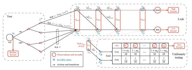
Figure 1: Schematic plot of a simplified version of our hard instance for $2$-step revealing POMDPs. The instance consists of three components: tree, lock, and uniformity testing. In the tree, all transitions are deterministic and fully observable, and the agent fully controls how to transit from $s_{0}$ to a leaf node. The tree transits stochastically to the lock if any action is taken at any leaf of the tree, but there is a unique (unknown) state $s^{\star}$, step $h^{\star}$, and action $a^{\star}$ at which the agent to transit to $s_{\oplus}$ with positive probability. In the lock, the agent cannot observe the latent states $\{s_{\oplus},s_{\ominus}\}$, and they need to enter the correct password $\mathbf{a}^{\star}$ to stay at $s_{\oplus}$ to eventually receive a high reward. The agent may also take the revealing action $a_{{\sf rev}}^{\star}$ at any $o_{\sf dum}$ to transit to the uniformity testing component, in which they will receive an observation that slightly reveals whether the previous latent state is $s_{\oplus}$ or $s_{\ominus}$. See Section 5.1 for a more detailed description.

5 Proof overview

We now provide a technical overview of the hard instance constructions and the lower bound proofs. We present a simplified version of the multi-step revealing hard instance in Appendix F that is used for proving both the PAC and the regret lower bounds (Theorem 3.2 & 4.1). For simplicity, we describe our construction in the 2-step case ($m=2$); a schematic plot of the resulting POMDP is given in Figure 1.

5.1 Construction of hard instance

A main challenge for obtaining our lower bounds—compared with existing lower bounds in fully observable settings—is to characterize the difficulty of partial observability, i.e. the dependence on $O$ and $\alpha^{-1}$.

2-step revealing combination lock

To reflect this difficulty, the basic component we design is a “2-step revealing combination lock” (cf. the “Lock” part in Figure 1), which is a modification of the non-revealing combination lock of Liu et al. (2022a); Jin et al. (2020a). This lock consists of two hidden states $s_{\oplus},s_{\ominus}$ and an (unknown) sequence of “correct” actions (i.e. the “password”) $\mathbf{a}^{\star}_{h^{\star}+1:H}$. The only way to stay at $s_{\oplus}$ is to take the correct action $\mathbf{a}^{\star}_{h}$ at each step $h$, and only state $s_{\oplus}$ at step $H$ gives a high reward. Therefore, the task of learning the optimal policy is equivalent to identifying the correct action $\mathbf{a}^{\star}_{h}$ at each step. We make the hidden states $s_{\oplus},s_{\ominus}$ non-observable (emit dummy observations $o_{\sf dum}$), so that a naive strategy for the agent is to guess the sequence $\mathbf{a}^{\star}$ from scratch, which incurs an $\exp(\Omega\!\left(H\right))$ sample complexity.

A central ingredient of our design is a unique (known) revealing action $a_{{\sf rev}}^{\star}$ at each step that is always distinct from the correct action. Taking $a_{{\sf rev}}^{\star}$ will transit from latent state $s_{\oplus}$ to $e_{\oplus}$ which then emits an observation from distribution $\mu_{\oplus}\in\Delta(\mathcal{O})$, and similarly from $s_{\ominus}$ to $e_{\ominus}$ which then emits an observation from distribution $\mu_{\ominus}\in\Delta(\mathcal{O})$. After this (single) emission, the system deterministically transits to an absorbing terminal state with reward $0$.

Uniformity testing

We adapt techniques from the uniformity testing (Canonne, 2020, 2022) literature to pick $\{\mu_{\oplus},\mu_{\ominus}\}$ that are as hard to distinguish as possible, yet ensuring that the POMDP still satisfies the $\alpha$-revealing condition. Concretely, picking $\mu_{\ominus}=\mathrm{Unif}(\mathcal{O})$ to be the uniform distribution over $\mathcal{O}$, it is known that testing $\mu_{\ominus}$ from a nearby $\mu_{\oplus}$ with $D_{\mathrm{TV}}\left(\mu_{\oplus},\mu_{\ominus}\right)\asymp\sigma$ requires $\Theta(\sqrt{O}/\sigma^{2})$ samples (Paninski, 2008). Further, the worst-case prior for $\mu_{\oplus}$ takes form $\mu_{\oplus}=\mathrm{Unif}(\mathcal{O})+\sigma\mu/O$, where $\mu\sim\mathrm{Unif}(\{(+1,-1),(-1,+1)\}^{O/2})$. We adopt such choices of $\mu_{\ominus}$ and $\mu_{\oplus}$ in our hard instance (cf. the “Uniformity testing” part in Figure 1), which can also ensure that the POMDP is $\Theta\!\left(\sigma^{-1}\right)$-revealing.

Tree MDP; rewards

To additionally exhibit an $HSA$ factor in the lower bound, we further embed a fully observable tree MDP (Domingues et al., 2021) before the combination lock. The tree is a balanced binary tree with $S$ leaf nodes, with deterministic transitions (so that which leaf node to arrive at is fully determined by the action sequence) and full observability. All leaf nodes of the tree will transit to the combination lock (i.e. one of ${\left\{s_{\oplus},s_{\ominus}\right\}}$). However, there exists a unique $(h^{\star},s^{\star},\mathbf{a}^{\star})$ such that only taking $a_{h^{\star}}=a^{\star}$ at $s_{h^{\star}}=s^{\star}$ and step $h^{\star}$ has a probability $\varepsilon$ of transiting to $s_{\oplus}$; all other choices at leaf nodes transit to $s_{\ominus}$ with probability one (cf. the “Tree” part in Figure 1).

We further design the reward function so that the agent must identify the underlying parameters $(h^{\star},s^{\star},a^{\star})$ correctly to learn a $\Theta(\varepsilon)$ near-optimal policy.

5.2 Calculation of lower bound

Base on our construction, to learn an $\varepsilon$ near-optimal policy in this hard instance, the agent has to identify $(h^{\star},s^{\star},a^{\star})$, which can only be achieved by trying all “entrances” $(s,a,h)$ and testing between

$$H_{0}: ~{}\mathbb{P}(s_{h+1}=s_{\oplus}|s_{h}=s,a_{h}=a)=0,$$

$$H_{1}: ~{}\mathbb{P}(s_{h+1}=s_{\oplus}|s_{h}=s,a_{h}=a)=\varepsilon.$$

for each entrance. As we have illustrated, to achieve this, the agent has to either (1) guess the password $\mathbf{a}^{\star}$ from scratch (using $\Omega\!\left(A^{H-h}/\varepsilon^{2}\right)$ samples), or (2) take $a_{{\sf rev}}^{\star}$ and perform uniformity testing using the observations. The latter task turns out to be equivalent to testing between

$$H_{0}^{\prime}=\mu_{\ominus},\quad H_{1}^{\prime}=\varepsilon\mu_{\oplus}+(1-\varepsilon)\mu_{\ominus},$$

where $\mu_{\ominus}$ is the uniform distribution over $2K=\Theta(O)$ elements, and $\mu_{\oplus}$ is drawn from the worst-case prior for uniformity testing. Distinguishing between $H_{0}^{\prime}$ and $H_{1}^{\prime}$ is a uniformity testing task with parameter $\sigma\varepsilon$, which requires $n\geq\Omega(\sqrt{O}/(\varepsilon\sigma)^{2})$ samples (Paninski, 2008).

With careful information-theoretic arguments, the arguments above will result in a PAC lower bound

$$\Theta\!\left(SAH\right)\times\Omega\Big{(}\min\Big{\{}\frac{\sqrt{O}}{\sigma^{2}\varepsilon^{2}},\frac{A^{\Theta\!\left(H\right)}}{\varepsilon^{2}}\Big{\}}\Big{)},$$

for learning 2-step $\Theta(\sigma^{-1})$-revealing POMDPs. This rate is similar as (though slightly worse than) our actual PAC lower bound (Theorem 3.2). The same hard instance further yields a $\Omega(T^{2/3})$ regret lower bound (though slightly worse rate than Theorem 4.1); see a calculation in Section F.8.

We remark that the above calculations are heuristic; rigorizing these arguments relies on information-theoretic arguments—in our case Ingster’s method (Ingster and Suslina, 2012) (cf. Appendix D & Lemma E.5 as an example)—for bounding the divergences between distributions induced by an arbitrary algorithm on different hard instances.

5.3 Remark on actual constructions

The above 2-step hard instance is a simplification of the actual ones used in the proofs of Theorem 3.2 & 4.1 in several aspects. The actual constructions are slightly more sophisticated, with the following additional ingredients:

• For the $m$-step case, to obtain a lower bound that scales with $A^{m}$, we modify the construction above so that the agent can take $a_{{\sf rev}}^{\star}$ only once per $(m-1)$-steps, and replace $a_{{\sf rev}}^{\star}$ by a set $|\mathcal{A}_{{\sf rev}}|=\Theta(A)$ of revealing actions, which collectively lead to an $A^{m-1}\times A=A^{m}$ factor.

• We further obtain an extra $\sqrt{S}$ factor in Theorem 3.2 by replacing the single combination lock with $\Theta(S)$ parallel locks that share the same password but differ in their emission probabilities. We show that learning in this setting is least as hard as uniformity testing over $\Theta(SO)$ elements, which leads to the extra $\sqrt{S}$ factor.

6 Discussions

6.1 Regret for single-step case

As we have discussed, single-step revealing POMDPs cannot possibly admit a $\Omega(T^{2/3})$ regret lower bound like the multi-step case, as a $\widetilde{\mathcal{O}}(\sqrt{T})$ upper bound is achievable. Nevertheless, we obtain a matching $\Omega(\sqrt{T})$ regret lower bound by a direct reduction from the PAC lower bound (Theorem 3.1) using Markov’s inequality and standard online-to-batch conversion, which we state as follows.

Corollary 6.1 (Regret lower bound for single-step revealing POMDPs).

Under the same setting as Theorem 3.1, the same family $\mathcal{M}$ of single-step $\alpha$-revealing POMDPs there satisfy that for any algorithm $\mathfrak{A}$,

$$\begin{aligned} \max_{M\in\mathcal{M}}\mathbb{E}^{\mathfrak{A}}_{M}{\left[\mathrm{\mathbf{Regret}}\right]}\geq c_{0}\cdot\min\Big{\{}\sqrt{\frac{SO^{1/2}AH}{\alpha^{2}}T},\sqrt{SA^{H/2}HT},T\Big{\}},\end{aligned}$$ (5)

where $c_{0}>0$ is an absolute constant.

To contrast this lower bound, the current best regret upper bound for single-step revealing POMDPs is $\widetilde{\mathcal{O}}(\sqrt{S^{3}O^{3}A^{2}(1+SA/O)\alpha^{-4}\cdot T}\times{\rm poly}(H))$ (Liu et al., 2022b), which is at least a $\sqrt{S^{2}O^{2.5}A\alpha^{-2}}$-factor larger than the main term in Equation 5. Here we present a much sharper regret upper bound, reducing this gap to $\sqrt{SO^{1.5}}$ and importantly settling the dependence on $\alpha$.

Theorem 6.2 (Regret upper bound for single-step revealing POMDPs).

There exists algorithms (OMLE, E2D-TA, and MOPS) that can interact with any single-step $\alpha$-revealing POMDP $M$ and achieve regret

$$\textstyle\mathrm{\mathbf{Regret}}\leq\widetilde{\mathcal{O}}\Big{(}\sqrt{\frac{S^{2}O^{2}A(1+SA/O)H^{3}}{\alpha^{2}}\cdot T}\Big{)}$$ (6)

with high probability.

We establish Theorem 6.2 on a broader class of sequential decision problems termed as strongly B-stable PSRs (cf. Section H.1), which include single-step revealing POMDPs as a special case. The proof is largely parallel to the analysis of PAC learning for B-stable PSRs (Chen et al., 2022a), and can be found in Appendix H.

6.2 Implications on the DEC approach

The Decision-Estimation Coefficient (DEC) (Foster et al., 2021) offers another potential approach for establishing sample complexity lower bounds for any general RL problem. However, here we demonstrate that for revealing POMDPs, any lower bound given by the DEC will necessarily be strictly weaker than our lower bounds.

For example, for PAC learning, the Explorative DEC (EDEC) of $m$-step revealing POMDPs is known to admit an upper bound ${\rm edec}_{\gamma}\leq\widetilde{\mathcal{O}}(SA^{m}H^{2}\alpha^{-2}/\gamma)$ (Chen et al. (2022a); see also Proposition C.2), and consequently any PAC lower bound obtained by lower bounding the EDEC is at most $\Omega(SA^{m}H^{2}\alpha^{-2}/\varepsilon^{2})$ (Chen et al., 2022b). Such a lower bound would be necessarily smaller than our Theorem 3.2 by at least a factor of $\sqrt{O}(1\vee\sqrt{S}/A)$, and importantly does not scale polynomially in $O$.

Our lower bounds have additional interesting implications on the DEC theory in that, while algorithms such as the E2D achieve sample complexity upper bounds in terms of the DEC and log covering number for the model class (Foster et al., 2021; Chen et al., 2022b), without further assumptions, this log covering number cannot be replaced by that of either the value class or the policy class, giving negative answers to the corresponding questions left open in Foster et al. (2021) (cf. Section I.1 for a detailed discussion).

6.3 Towards closing the gaps

Finally, as an important open question, our lower bounds still have mild gaps from the current best upper bounds, importantly in the $(S,O)$ dependence. For example, for multi-step revealing POMDPs, the (first term in the) PAC lower bound $\Omega(S^{1.5}\sqrt{O}A^{m-1}/(\alpha^{2}\varepsilon^{2}))$ (Theorem 3.2) still has a $\sqrt{SO}A$ gap from the upper bound (Theorem 2.3). While we believe that the $A$ factor is an analysis artifact that may be removed, the remaining $\sqrt{SO}$ factor cannot be obtained in the lower bound if we stick to the current family of hard instances—There exists an algorithm specially tailored to this family that achieves an $\widetilde{\mathcal{O}}(S^{1.5}\sqrt{O}A^{m}/(\alpha^{2}\varepsilon^{2}))$ upper bound, by brute-force enumeration in the tree and uniformity testing in the combination lock (Appendix I.2).

Closing this $\sqrt{SO}$ gap may require either stronger lower bounds with alternative hard instances—e.g. by embedding other problems in distribution testing (Canonne, 2020)—or sharper upper bounds, which we leave as future work.

7 Conclusion

This paper establishes sample complexity lower bounds for partially observable reinforcement learning in the important tractable class of revealing POMDPs. Our lower bounds are the first to scale polynomially in the number of states, actions, observations, and the revealing constant in a multiplicative fashion, and suggest rather mild gaps between the lower bounds and current best upper bounds. Our work provides a strong foundation for future fine-grained studies and opens up many interesting questions, such as closing the gaps (from either side), or strengthening the multi-step revealing assumption meaningfully to allow a $\sqrt{T}$ regret.

Appendix A Technical tools

Lemma A.1.

For positive real numbers $A,B,T,\varepsilon_{0}>0$, it holds that

$$\sup_{\varepsilon\in(0,\varepsilon_{0}]}{\left(\varepsilon T\wedge\frac{A}{\varepsilon^{2}}\wedge\frac{B}{\varepsilon}\right)}\geq A^{1/3}T^{2/3}\wedge\sqrt{BT}\wedge\varepsilon_{0}T.$$

Proof of Lemma A.1.

Suppose that $R>0$ is such that $R\geq\varepsilon T\wedge\frac{A}{\varepsilon^{2}}\wedge\frac{B}{\varepsilon}$ for all $\varepsilon\in(0,\varepsilon_{0}]$. Then for each $\varepsilon\in(0,\varepsilon_{0}]$, either $\varepsilon\leq\frac{R}{T}$, or $\varepsilon\geq\sqrt{\frac{A}{R}}$, or $\varepsilon\geq\frac{B}{R}$. Thus,

$$(0,\varepsilon_{0}]\subseteq(0,\frac{R}{T}]\cup[\sqrt{\frac{A}{R}},+\infty)\cup[\frac{B}{R},+\infty).$$

Therefore, either $\frac{R}{T}\geq\varepsilon_{0}$, or $\sqrt{\frac{A}{R}}\leq\frac{R}{T}$, or $\frac{B}{R}\leq\frac{R}{T}$. Combining these three cases together, we obtain

$$R\geq\varepsilon_{0}T\wedge A^{1/3}T^{2/3}\wedge\sqrt{BT}.$$

∎

Lemma A.2.

Suppose that $(R_{t})_{t\geq 1}$ is a sequence of positive random variables adapted to filtration $(\mathcal{F}_{t})_{t\geq 1}$ and $\mathsf{T}$ is a stopping time (i.e. for $t\geq 1$, $R_{t}$ is $\mathcal{F}_{t}$-measurable and the event ${\left\{\mathsf{T}\leq t\right\}}\in\mathcal{F}_{t}$). Then it holds that

$$\mathbb{E}{\left[\prod_{t=1}^{\mathsf{T}}R_{t}\times\prod_{t=1}^{\mathsf{T}}\mathbb{E}[R_{t}|\mathcal{F}_{t-1}]^{-1}\right]}=1.$$

Equivalently,

$$\mathbb{E}{\left[\prod_{t=1}^{\mathsf{T}}R_{t}\times\exp{\left(-\sum_{t=1}^{\mathsf{T}}\log\mathbb{E}[R_{t}|\mathcal{F}_{t-1}]\right)}\right]}=1.$$

Lemma A.2 follows immediately from iteratively applications of the tower properties.

Lemma A.3.

Suppose that random variable $X$ is $\sigma$-sub-Gaussian, i.e. $\mathbb{E}{\left[\exp(tX)\right]}\leq\exp{\left(\frac{\sigma^{2}t^{2}}{2}\right)}$ for any $t\in\mathbb{R}$. Then for all $t\geq 0$, we have

$$\mathbb{E}{\left[\exp(t\left|X\right|)\right]}\leq\exp{\left(\max{\left\{\sigma^{2}t^{2},\frac{4}{3}\sigma t\right\}}\right)}.$$

Proof of Lemma A.3.

For any $x\geq 1$, we have

$$\mathbb{E}{\left[\exp(t\left|X\right|)\right]}\leq\mathbb{E}{\left[\exp(xt\left|X\right|)\right]}^{\frac{1}{x}}\leq{\left(\mathbb{E}{\left[\exp(xtX)\right]}+\mathbb{E}{\left[\exp(-xtX)\right]}\right)}^{\frac{1}{x}}\leq 2^{\frac{1}{x}}\exp{\left(\frac{\sigma^{2}t^{2}x}{2}\right)}=\exp{\left(\frac{\sigma^{2}t^{2}x}{2}+\frac{\log 2}{x}\right)}.$$

We consider two cases: 1. If $\sigma t\geq\sqrt{2\log 2}$, then by taking $x=1$ in the above inequality, we have $\mathbb{E}{\left[\exp(t\left|X\right|)\right]}\leq\exp(\sigma^{2}t^{2})$. 2. If $\sigma t<\sqrt{2\log 2}$, then by taking $x=\frac{\sqrt{2\log 2}}{\sigma t}>1$ in the above inequality, we have $\mathbb{E}{\left[\exp(t\left|X\right|)\right]}\leq\exp(\sqrt{2\log 2}\sigma t)\leq\exp(\frac{4}{3}\sigma t)$. Combining these two cases completes the proof. ∎

For probability distributions $\mathbb{P}$ and $\mathbb{Q}$ on a measurable space $(\mathcal{X},\mathcal{F})$ with a base measure $\mu$, we define the TV distance and the Hellinger distance between $\mathbb{P},\mathbb{Q}$ as

$$D_{\mathrm{TV}}\left(\mathbb{P},\mathbb{Q}\right) =\sup_{A\in\mathcal{F}}\left|\mathbb{P}(A)-\mathbb{Q}(A)\right|=\frac{1}{2}\int_{\mathcal{X}}\left|\frac{d\mathbb{P}}{d\mu}(x)-\frac{d\mathbb{Q}}{d\mu}(x)\right|d\mu(x),$$

$$D_{\mathrm{H}}^{2}\left(\mathbb{P},\mathbb{Q}\right) =\int_{\mathcal{X}}{\left(\sqrt{\frac{d\mathbb{P}}{d\mu}}-\sqrt{\frac{d\mathbb{Q}}{d\mu}}\right)}^{2}d\mu.$$

When $\mathbb{P}\ll\mathbb{Q}$, we can also define the KL-divergence and the $\chi^{2}$-divergence between $\mathbb{P},\mathbb{Q}$ as

$$\operatorname{KL}(\mathbb{P}\;\|\;\mathbb{Q})=\mathbb{E}_{\mathbb{P}}{\left[\log{\frac{d\mathbb{P}}{d\mathbb{Q}}}\right]},\qquad\chi^{2}(\mathbb{P}\;\|\;\mathbb{Q})=\mathbb{E}_{\mathbb{Q}}{\left[{\left(\frac{d\mathbb{P}}{d\mathbb{Q}}\right)}^{2}\right]}-1.$$

Lemma A.4.

Suppose $\mathbb{P},\mathbb{Q},\mathbb{P}^{\prime},\mathbb{Q}^{\prime}$ are four probability measures on $(\mathcal{X},\mathcal{F})$, and $\Omega$ is an event such that $\mathbb{P}|_{\Omega}=\mathbb{P}^{\prime}|_{\Omega}$, $\mathbb{Q}|_{\Omega}=\mathbb{Q}^{\prime}|_{\Omega}$. Then it holds that

$$D_{\mathrm{TV}}\left(\mathbb{P}^{\prime},\mathbb{Q}^{\prime}\right)\geq D_{\mathrm{TV}}\left(\mathbb{P},\mathbb{Q}\right)-\mathbb{P}(\Omega^{c}).$$

Proof of Lemma A.4.

Let $\mu$ be a base measure on $(\mathcal{X},\mathcal{F})$ such that $\mathbb{P},\mathbb{P}^{\prime},\mathbb{Q},\mathbb{Q}^{\prime}$ have densities with respect to $\mu$ (for example, $\mu=(\mathbb{P}+\mathbb{P}^{\prime}+\mathbb{Q}+\mathbb{Q}^{\prime})/4$). For notation simplicity, we use $\mathbb{P}(x)$ to stand for $d\mathbb{P}(x)/d\mu(x)$ and use $dx$ to stand for $\mu(dx)$. Then we have

$$2D_{\mathrm{TV}}\left(\mathbb{P}^{\prime},\mathbb{Q}^{\prime}\right)= \int_{\mathcal{X}}\left|\mathbb{P}^{\prime}(x)-\mathbb{Q}^{\prime}(x)\right|dx=\int_{\Omega}\left|\mathbb{P}^{\prime}(x)-\mathbb{Q}^{\prime}(x)\right|dx+\int_{\Omega^{c}}\left|\mathbb{P}^{\prime}(x)-\mathbb{Q}^{\prime}(x)\right|dx$$

$$\geq \int_{\Omega}\left|\mathbb{P}^{\prime}(x)-\mathbb{Q}^{\prime}(x)\right|dx+\left|\mathbb{P}^{\prime}(\Omega^{c})-\mathbb{Q}^{\prime}(\Omega^{c})\right|$$

$$= \int_{\Omega}\left|\mathbb{P}(x)-\mathbb{Q}(x)\right|dx+\left|\mathbb{P}(\Omega^{c})-\mathbb{Q}(\Omega^{c})\right|$$

$$\geq \int_{\Omega}\left|\mathbb{P}(x)-\mathbb{Q}(x)\right|dx+\mathbb{P}(\Omega^{c})+\mathbb{Q}(\Omega^{c})-2\mathbb{P}(\Omega^{c})$$

$$\geq \int_{\Omega}\left|\mathbb{P}(x)-\mathbb{Q}(x)\right|dx+\int_{\Omega^{c}}\left|\mathbb{P}(x)-\mathbb{Q}(x)\right|dx-2\mathbb{P}(\Omega^{c})$$

$$= 2D_{\mathrm{TV}}\left(\mathbb{P},\mathbb{Q}\right)-2\mathbb{P}(\Omega^{c}).$$

This completes the proof. ∎

Lemma A.5 (Divergence inequalities, see e.g. Sason and Verdú (2016)).

For two probability measures $\mathbb{P},\mathbb{Q}$ on $(\mathcal{X},\mathcal{F})$, it holds that

$$2D_{\mathrm{TV}}\left(\mathbb{P},\mathbb{Q}\right)^{2}\leq\operatorname{KL}(\mathbb{P}\;\|\;\mathbb{Q})\leq\log{\left(1+\chi^{2}(\mathbb{P}\;\|\;\mathbb{Q})\right)}.$$

Lemma A.6 (Hellinger conditioning lemma, see e.g. Chen et al. (2022a, Lemma A.1)).

For any pair of random variables $(X,Y)$, it holds that

$$\mathbb{E}_{X\sim\mathbb{P}_{X}}{\left[D_{\mathrm{H}}^{2}\left(\mathbb{P}_{Y|X},\mathbb{Q}_{Y|X}\right)\right]}\leq 2D_{\mathrm{H}}^{2}\left(\mathbb{P}_{X,Y},\mathbb{Q}_{X,Y}\right).$$

Appendix B Basics of predictive state representations and B-stability

The following notations for predictive state representations (PSRs) and the B-stability condition are extracted from (Chen et al., 2022a).

Sequential decision processes with observations

An episodic sequential decision process is specified by a tuple ${\left\{H,\mathcal{O},\mathcal{A},\mathbb{P},\{r_{h}\}_{h\in[H]}\right\}}$, where $H\in\mathbb{Z}_{\geq 1}$ is the horizon length; $\mathcal{O}$ is the observation space; $\mathcal{A}$ is the action space; $\mathbb{P}$ specifies the transition dynamics, such that the initial observation follows $o_{1}\sim\mathbb{P}_{0}(\cdot)\in\Delta(\mathcal{O})$, and given the history $\tau_{h}\mathrel{\mathop{:}}=(o_{1},a_{1},\cdots,o_{h},a_{h})$ up to step $h$, the observation follows $o_{h+1}\sim\mathbb{P}(\cdot|\tau_{h})$; $r_{h}:\mathcal{O}\times\mathcal{A}\to[0,1]$ is the reward function at $h$-th step, which we assume is a known deterministic function of $(o_{h},a_{h})$.

In an episodic sequential decision process, a policy $\pi=\{\pi_{h}:(\mathcal{O}\times\mathcal{A})^{h-1}\times\mathcal{O}\to\Delta(\mathcal{A})\}_{h\in[H]}$ is a collection of $H$ functions. At step $h\in[H]$, an agent running policy $\pi$ observes the observation $o_{h}$ and takes action $a_{h}\sim\pi_{h}(\cdot|\tau_{h-1},o_{h})\in\Delta(\mathcal{A})$ based on the history $(\tau_{h-1},o_{h})=(o_{1},a_{1},\dots,o_{h-1},a_{h-1},o_{h})$. The agent then receives their reward $r_{h}(o_{h},a_{h})$, and the environment generates the next observation $o_{h+1}\sim\mathbb{P}(\cdot|\tau_{h})$ based on $\tau_{h}=(o_{1},a_{1},\cdots,o_{h},a_{h})$ (if $h<H$). The episode terminates immediately after $a_{H}$ is taken.

For any $\tau_{h}=(o_{1},a_{1},\cdots,o_{h},a_{h})$, we write

$$\mathbb{P}(\tau_{h})\mathrel{\mathop{:}}= ~{}\mathbb{P}(o_{1:h}|a_{1:h})=\prod_{h^{\prime}\leq h}\mathbb{P}(o_{h^{\prime}}|\tau_{h^{\prime}-1}),$$

$$\pi(\tau_{h})\mathrel{\mathop{:}}= ~{}\prod_{h^{\prime}\leq h}\pi_{h^{\prime}}(a_{h^{\prime}}|\tau_{h^{\prime}-1},o_{h^{\prime}}),$$

$$\mathbb{P}^{\pi}(\tau_{h})\mathrel{\mathop{:}}= ~{}\mathbb{P}(\tau_{h})\times\pi(\tau_{h}).$$

Then $\mathbb{P}^{\pi}(\tau_{h})$ is the probability of observing $\tau_{h}$ (for the first $h$ steps) when executing $\pi$.

PSR, core test sets, and predictive states

A test $t$ is a sequence of future observations and actions (i.e. $t\in\mathfrak{T}:=\bigcup_{W\in\mathbb{Z}_{\geq 1}}\mathcal{O}^{W}\times\mathcal{A}^{W-1}$). For some test $t_{h}=(o_{h:h+W-1},a_{h:h+W-2})$ with length $W\geq 1$, we define the probability of test $t_{h}$ being successful conditioned on (reachable) history $\tau_{h-1}$ as $\mathbb{P}(t_{h}|\tau_{h-1})\mathrel{\mathop{:}}=\mathbb{P}(o_{h:h+W-1}|\tau_{h-1};\mathrm{do}(a_{h:h+W-2}))$, i.e., the probability of observing $o_{h:h+W-1}$ if the agent deterministically executes actions $a_{h:h+W-2}$, conditioned on history $\tau_{h-1}$. We follow the convention that, if $\mathbb{P}^{\pi}(\tau_{h-1})=0$ for any $\pi$, then $\mathbb{P}(t|\tau_{h-1})=0$.

Definition B.1 (PSR, core test sets, and predictive states).

For any $h\in[H]$, we say a set ${\mathcal{U}_{h}}\subset\mathfrak{T}$ is a core test set at step $h$ if the following holds: For any $W\in\mathbb{Z}_{\geq 1}$, any possible future (i.e., test) $t_{h}=(o_{h:h+W-1},a_{h:h+W-2})\in\mathcal{O}^{W}\times\mathcal{A}^{W-1}$, there exists a vector $b_{t_{h},h}\in\mathbb{R}^{{\mathcal{U}_{h}}}$ such that

$$\mathbb{P}(t_{h}|\tau_{h-1})=\langle b_{t_{h},h},[\mathbb{P}(t|\tau_{h-1})]_{t\in{\mathcal{U}_{h}}}\rangle,\qquad\forall\tau_{h-1}\in\mathcal{T}^{h-1}:=(\mathcal{O}\times\mathcal{A})^{h-1}.$$ (7)

We refer to the vector $\mathbf{q}(\tau_{h-1})\mathrel{\mathop{:}}=[\mathbb{P}(t|\tau_{h-1})]_{t\in{\mathcal{U}_{h}}}$ as the predictive state at step $h$ (with convention $\mathbf{q}(\tau_{h-1})=0$ if $\tau_{h-1}$ is not reachable), and $\mathbf{q}_{0}\mathrel{\mathop{:}}=[\mathbb{P}(t)]_{t\in\mathcal{U}_{1}}$ as the initial predictive state. A (linear) PSR is a sequential decision process equipped with a core test set $\{{\mathcal{U}_{h}}\}_{h\in[H]}$.

Define $\mathcal{U}_{A,h}\mathrel{\mathop{:}}=\{\mathbf{a}:(\mathbf{o},\mathbf{a})\in{\mathcal{U}_{h}}~{}\textrm{for some}~{}\mathbf{o}\in\bigcup_{W\in\mathbb{N}^{+}}\mathcal{O}^{W}\}$ as the set of “core actions” (possibly including an empty sequence) in ${\mathcal{U}_{h}}$, with $U_{A}\mathrel{\mathop{:}}=\max_{h\in[H]}\left|\mathcal{U}_{A,h}\right|$. Further define $\mathcal{U}_{H+1}\mathrel{\mathop{:}}={\left\{o_{\rm dum}\right\}}$ for notational simplicity. The core test sets $({\mathcal{U}_{h}})_{h\in[H]}$ are assumed to be known and the same within a PSR model class.

Definition B.2 (PSR rank).

Given a PSR, its PSR rank is defined as $d_{\sf PSR}:=\max_{h\in[H]}\mathrm{rank}(D_{h})$, where $D_{h}:=\left[\mathbf{q}(\tau_{h})\right]_{\tau_{h}\in\mathcal{T}^{h}}\in\mathbb{R}^{{\mathcal{U}_{h+1}}\times\mathcal{T}^{h}}$ is the matrix formed by predictive states at step $h\in[H]$.

For POMDP, it is clear that $d_{\sf PSR}\leq S$, regardless of the core test sets.

B-representation

(Chen et al., 2022a) introduced the notion of B-representation of PSR, which plays a fundamental role in their general structural condition and their analysis.

Definition B.3 (B-representation).

A B-representation of a PSR with core test set $({\mathcal{U}_{h}})_{h\in[H]}$ is a set of matrices $\{(\mathbf{B}_{h}(o_{h},a_{h})\in\mathbb{R}^{{\mathcal{U}_{h+1}}\times{\mathcal{U}_{h}}})_{h,o_{h},a_{h}},\mathbf{q}_{0}\in\mathbb{R}^{\mathcal{U}_{1}}\}$ such that for any $0\leq h\leq H$, policy $\pi$, history $\tau_{h}=(o_{1:h},a_{1:h})\in\mathcal{T}^{h}$, and core test $t_{h+1}=(o_{h+1:h+W},a_{h+1:h+W-1})\in{\mathcal{U}_{h+1}}$, the quantity $\mathbb{P}(\tau_{h},t_{h+1})$, i.e. the probability of observing $o_{1:h+W}$ upon taking actions $a_{1:h+W-1}$, admits the decomposition

$$\mathbb{P}(\tau_{h},t_{h+1})=\mathbb{P}(o_{1:h+W}|\mathrm{do}(a_{1:h+W-1}))=\mathbf{e}_{t_{h+1}}^{\top}\cdot\mathbf{B}_{h:1}(\tau_{h})\cdot\mathbf{q}_{0},$$ (8)

where $\mathbf{e}_{t_{h+1}}\in\mathbb{R}^{{\mathcal{U}_{h+1}}}$ is the indicator vector of $t_{h+1}\in{\mathcal{U}_{h+1}}$, and

$$\mathbf{B}_{h:1}(\tau_{h})\mathrel{\mathop{:}}=\mathbf{B}_{h}(o_{h},a_{h})\mathbf{B}_{h-1}(o_{h-1},a_{h-1})\cdots\mathbf{B}_{1}(o_{1},a_{1}).$$

Based on the B-representations of PSRs, Chen et al. (2022a) proposed the following structural condition for sample-efficient learning in PSRs.

Definition B.4 (B-stability (Chen et al., 2022a)).

A PSR is B-stable with parameter $\Lambda_{\sf B}\geq 1$ (henceforth also $\Lambda_{\sf B}$-stable) if it admits a B-representation such that for all step $h\in[H]$, policy $\pi$, and $x\in\mathbb{R}^{{\mathcal{U}_{h}}}$, we have

$$\sum_{\tau_{h:H}=(o_{h},a_{h},\cdots,o_{H},a_{H})}\pi(\tau_{h:H})\times\left|\mathbf{B}_{H}(o_{H},a_{H})\cdots\mathbf{B}_{h}(o_{h},a_{h})x\right|\leq\Lambda_{\sf B}\max{\left\{\left\|x\right\|_{*},\left\|x\right\|_{\Pi^{\prime}}\right\}},$$ (9)

where for any vector $x=(x(t))_{t\in{\mathcal{U}_{h}}}$, we denote its $(1,2)$-norm by

$$\textstyle\left\|x\right\|_{*}\mathrel{\mathop{:}}=\big{(}\sum_{\mathbf{a}\in\mathcal{U}_{A,h}}\big{(}\sum_{\mathbf{o}:(\mathbf{o},\mathbf{a})\in{\mathcal{U}_{h}}}|x(\mathbf{o},\mathbf{a})|\big{)}^{2}\big{)}^{1/2},$$

and its $\Pi^{\prime}$-norm by

$$\textstyle\left\|x\right\|_{\Pi^{\prime}}\mathrel{\mathop{:}}=\max_{\bar{\pi}}\sum_{t\in\overline{\mathcal{U}}_{h}}\bar{\pi}(t)\left|x(t)\right|,$$

where $\overline{\mathcal{U}}_{h}\mathrel{\mathop{:}}=\{t\in{\mathcal{U}_{h}}:\not\exists t^{\prime}\in{\mathcal{U}_{h}}\text{ such that $t$ is a prefix of $t^{\prime}$}\}$.

Equivalently, (9) can be written as $\left\|\mathcal{B}x\right\|_{\Pi}\leq\Lambda_{\sf B}\max{\left\{\left\|x\right\|_{*},\left\|x\right\|_{\Pi^{\prime}}\right\}}$, where for each step $h$, vector $x\in\mathbb{R}^{{\mathcal{U}_{h}}}$, we write

$$\left\|\mathcal{B}_{H:h}x\right\|_{\Pi}\mathrel{\mathop{:}}=\max_{\pi}\sum_{\tau_{h:H}}\pi(\tau_{h:H})\times\left|\mathbf{B}_{H:h}(\tau_{h:H})x\right|.$$ (10)

Chen et al. (2022a) showed that B-stability enables sample efficiency of PAC-learning, and we summarize the results in the following theorem.

Theorem B.5 (PAC upper bound for learning PSRs).

Suppose $\Theta$ is a PSR class with the same core test sets $\{{\mathcal{U}_{h}}\}_{h\in[H]}$, and each $\theta\in\Theta$ admits a B-representation that is $\Lambda_{\sf B}$-stable and has PSR rank at most $d$. Then there exists algorithms (OMLE/Explorative E2D/MOPS) that can find an $\varepsilon$-optimal policy with probability at least $1-\delta$, within

$$T\leq\widetilde{\mathcal{O}}\!\left(\frac{\Lambda_{\sf B}^{2}dAU_{A}H^{2}\log(\mathcal{N}_{\Theta}(1/T)/\delta)}{\varepsilon^{2}}\right)$$ (11)

episodes of play, where $\mathcal{N}_{\Theta}$ is the covering number of $\Theta$ (cf. Chen et al. (2022a, Definition A.4)).

When $\Theta$ is a subclass of POMDPs, we have $\log\mathcal{N}_{\Theta}(1/T)=\widetilde{\mathcal{O}}\!\left(H(S^{2}A+SO)\right)$ (Chen et al., 2022a). Therefore, to deduce Theorem 2.3 from the above general theorem, it remains to upper bound $\Lambda_{\sf B}$ for $m$-step $\alpha$-revealing POMDPs, which is done in Section C.2.

Appendix C Proofs for Section 2

C.1 Proof of Proposition 2.2

Fix any POMDP $M$, and we first show that $\alpha_{m+1}(M)\geq\alpha_{m}(M)$. By the definition of $\alpha_{m+1}(M)$ (Definition 2.1), it suffices to show the following result.

Lemma C.1.

For any $h\in[H-m]$, and any choice of generalized left inverse $\mathbb{M}_{h,m}^{+}$ (of $\mathbb{M}_{h,m}$), the matrix $\mathbb{M}_{h,m+1}$ admits a generalized left inverse $\mathbb{M}_{h,m+1}^{+}$ such that

$$\left\|\mathbb{M}_{h,m+1}^{+}\right\|_{*\to 1}\leq\left\|\mathbb{M}_{h,m}^{+}\right\|_{*\to 1}.$$

The converse part of Proposition 2.2 can be shown directly by examples. In particular, our construction in Appendix F readily provides such an example (see Remark F.10).

Proof of Lemma C.1.

Fix an arbitrary action $\widetilde{a}\in\mathcal{A}$. Consider the matrix $F_{\widetilde{a}}\in\mathbb{R}^{\mathcal{O}^{m}\mathcal{A}^{m-1}\times\mathcal{O}^{m+1}\mathcal{A}^{m}}$ defined as (the unique matrix associated with) the following linear operator:

$${\left[F_{\widetilde{a}}\mathbf{x}\right]}(\mathbf{o}_{h:h+m-1},\mathbf{a}_{h:h+m-2})\mathrel{\mathop{:}}=\sum_{o\in\mathcal{O}}\mathbf{x}(\mathbf{o}_{h:h+m-1}o,\mathbf{a}_{h:h+m-2}\widetilde{a}),\quad\textrm{for all}\;\mathbf{x}\in\mathbb{R}^{\mathcal{O}^{m+1}\mathcal{A}^{m}}.$$

We first show that $F_{\widetilde{a}}\mathbb{M}_{h,m+1}=\mathbb{M}_{h,m}$. Indeed,

$$\quad{\left[F_{\widetilde{a}}\mathbb{M}_{h,m+1}\right]}_{\mathbf{o}_{h:h+m-1}\mathbf{a}_{h:h+m-2},s}=\sum_{o\in\mathcal{O}}{\left[\mathbb{M}_{h,m+1}\right]}_{(\mathbf{o}_{h:h+m-1}o)(\mathbf{a}_{h:h+m-2}\widetilde{a}),s}$$

$$=\sum_{o\in\mathcal{O}}\mathbb{P}{\left(o_{h:h+m}=\mathbf{o}_{h:h+m-1}o|a_{h:h+m-1}=\mathbf{a}_{h:h+m-2}\widetilde{a},s_{h}=s\right)}$$

$$=\mathbb{P}{\left(o_{h:h+m-1}=\mathbf{o}_{h:h+m-1}|a_{h:h+m-2}=\mathbf{a}_{h:h+m-2},s_{h}=s\right)}={\left[\mathbb{M}_{h,m}\right]}_{\mathbf{o}_{h:h+m-1}\mathbf{a}_{h:h+m-2},s}$$

for any $(\mathbf{o}_{h:h+m-1}\mathbf{a}_{h:h+m-2},s)$, which verifies the claim. Therefore, for any generalized left inverse $\mathbb{M}_{h,m}^{+}$, we can take

$$\mathbb{M}_{h,m+1}^{+}\mathrel{\mathop{:}}=\mathbb{M}_{h,m}^{+}F_{\widetilde{a}}.$$

This matrix satisfies $\mathbb{M}_{h,m+1}^{+}\mathbb{M}_{h,m+1}\mathbb{T}_{h-1}=\mathbb{M}_{h,m}^{+}F_{\widetilde{a}}\mathbb{M}_{h,m+1}\mathbb{T}_{h-1}=\mathbb{M}_{h,m}^{+}\mathbb{M}_{h,m}\mathbb{T}_{h-1}=\mathbb{T}_{h-1}$ and is thus indeed a generalized left inverse of $\mathbb{M}_{h,m+1}$. Further,

$$\left\|\mathbb{M}_{h,m+1}^{+}\right\|_{*\to 1}=\left\|\mathbb{M}_{h,m}^{+}F_{\widetilde{a}}\right\|_{*\to 1}\leq\left\|\mathbb{M}_{h,m}^{+}\right\|_{*\to 1}\left\|F_{\widetilde{a}}\right\|_{*\to*},$$

so it remains to show that $\left\|F_{\widetilde{a}}\right\|_{*\to*}\leq 1$. To see this, note that for any $\mathbf{x}\in\mathbb{R}^{\mathcal{O}^{m+1}\mathcal{A}^{m}}$ with $\left\|\mathbf{x}\right\|_{*}^{2}\leq 1$, we have

$$\quad\left\|F_{\widetilde{a}}\mathbf{x}\right\|_{*}^{2}=\sum_{\mathbf{a}_{h:h+m-2}\in\mathcal{A}^{m-1}}{\left(\sum_{\mathbf{o}_{h:h+m-1}\in\mathcal{O}^{m}}\left|\sum_{o\in\mathcal{O}}\mathbf{x}(\mathbf{o}_{h:h+m-1}o,\mathbf{a}_{h:h+m-2}\widetilde{a})\right|\right)}^{2}$$

$$\leq\sum_{\mathbf{a}_{h:h+m-2}\in\mathcal{A}^{m-1}}{\left(\sum_{\mathbf{o}_{h:h+m}\in\mathcal{O}^{m+1}}\left|\mathbf{x}(\mathbf{o}_{h:h+m},\mathbf{a}_{h:h+m-2}\widetilde{a})\right|\right)}^{2}$$

$$\leq\sum_{\mathbf{a}_{h:h+m-1}\in\mathcal{A}^{m}}{\left(\sum_{\mathbf{o}_{h:h+m}\in\mathcal{O}^{m+1}}\left|\mathbf{x}(\mathbf{o}_{h:h+m},\mathbf{a}_{h:h+m-1})\right|\right)}^{2}=\left\|\mathbf{x}\right\|_{*}^{2}.$$

This proves $\left\|F_{\widetilde{a}}\right\|_{*\to*}\leq 1$ and thus the desired result. ∎

C.2 Proof of Theorem 2.3

We will deduce Theorem 2.3 from the general result (Theorem B.5) of learning PSRs (Chen et al., 2022a). To apply Theorem B.5, we first invoke the following proposition, which basically states that any $m$-step $\alpha$-revealing POMDP is B-stable with $\Lambda_{\sf B}\leq\alpha^{-1}$.

Proposition C.2.

Any $m$-step $\alpha$-revealing POMDP is a $\alpha^{-1}$-stable PSR with core test set ${\mathcal{U}_{h}}=(\mathcal{O}\times\mathcal{A})^{\min{\left\{m-1,H-h\right\}}}\times\mathcal{O}$, i.e. it admits a $\Lambda_{\sf B}\leq\alpha^{-1}$-stable B-representation.

Therefore, for $\mathcal{M}$ a class of $m$-step $\alpha$-revealing POMDPs, $\mathcal{M}$ is also a class of PSRs with common core test sets, such that each $M\in\mathcal{M}$ is $\alpha^{-1}$-stable, has PSR rank at most $S$ and $U_{A}=A^{m-1}$. Then, Theorem B.5 implies that an $\varepsilon$-optimal policy of $\mathcal{M}$ can be learned using OMLE, Explorative E2D, or MOPS, with sample complexity

$$\widetilde{\mathcal{O}}\!\left(\frac{SA^{m}H^{2}\log(\mathcal{N}_{\mathcal{M}}(1/T)/\delta)}{\alpha^{2}\varepsilon^{2}}\right),$$

and we also have $\log\mathcal{N}_{\mathcal{M}}(1/T)=\widetilde{\mathcal{O}}\!\left(H(S^{2}A+SO)\right)$ (Chen et al., 2022a). Combining these facts completes the proof of Theorem 2.3. ∎

Proof of Proposition C.2.

Chen et al. (2022a, Appendix B.3.3) showed that any $m$-step $\alpha$-revealing POMDP $M$ is a $\alpha^{-1}$-stable PSR with core test set ${\mathcal{U}_{h}}=(\mathcal{O}\times\mathcal{A})^{\min{\left\{m-1,H-h\right\}}}\times\mathcal{O}$, and explicitly constructed the following B-representation for it: when $h\leq H-m$, set

$$\mathbf{B}_{h}(o,a)=\mathbb{M}_{h+1}\mathbb{T}_{h,a}\operatorname{diag}{\left(\mathbb{O}_{h}(o|\cdot)\right)}\mathbb{M}_{h}^{+},\qquad h\in[H-m],$$ (12)

and when $h>H-m$, take

$$\mathbf{B}_{h}(o_{h},a_{h})={\left[\mathbbm{1}{\left(t_{h}=(o_{h},a_{h},t_{h+1})\right)}\right]}_{(t_{h+1},t_{h})\in{\mathcal{U}_{h+1}}\times{\mathcal{U}_{h}}}\in\mathbb{R}^{{\mathcal{U}_{h+1}}\times{\mathcal{U}_{h}}},$$ (13)

where $\mathbbm{1}{\left(t_{h}=(o_{h},a_{h},t_{h+1})\right)}$ is 1 if $t_{h}$ equals to $(o_{h},a_{h},t_{h+1})$, and 0 otherwise.

Then, by Chen et al. (2022a, Lemma B.13), for any $1\leq h\leq H$, $x\in\mathbb{R}^{\left|{\mathcal{U}_{h}}\right|}$, it holds that

$$\left\|\mathcal{B}_{H:h}x\right\|_{\Pi}=\max_{\pi}\sum_{\tau_{h:H}}\left\|\mathbf{B}_{H}(o_{H},a_{H})\cdots\mathbf{B}_{h}(o_{h},a_{h})x\right\|_{1}\times\pi(\tau_{h:H})\leq\max{\left\{\left\|{\mathbb{M}_{h}^{+}x}\right\|_{1},\left\|x\right\|_{\Pi^{\prime}}\right\}}\leq\alpha^{-1}\max{\left\{\left\|x\right\|_{*},\left\|x\right\|_{\Pi^{\prime}}\right\}}.$$

Therefore, B-representation provided in (12) and (13) is indeed $\alpha^{-1}$-stable, and hence completes the proof. ∎

Appendix D Basics of Ingster’s method

In this section, we first introduce the basic notations frequently used in our analysis of hard instances, and then state Ingster’s method for proving information-theoretic lower bounds Ingster and Suslina (2012). Recall that we have introduced the formulation of sequential decision process in Appendix B.

Algorithms for sequential decision processes

An algorithm $\mathfrak{A}$ for sequential decision processes (with a fixed number of episodes $T$) is specified by a collection of $HT$ functions $\mathfrak{A}=\{\pi^{\mathfrak{A}}_{t,h}\}_{h\in[H],t\in[T]}$, where $\pi^{\mathfrak{A}}_{t,h}$ maps the tuple of all past histories and the current observation $(\tau^{(1)},\cdots,\tau^{(t-1)},\tau_{h-1}^{(t)},o_{h}^{(t)})$ to a distribution over actions $\Delta(\mathcal{A})$ from which we sample the next action $a_{h}^{(t)}\sim\pi^{\mathfrak{A}}_{t,h}(\cdot|\tau^{(1:t-1)},\tau_{h-1}^{(t)},o_{h}^{(t)})$. At the end of interaction, the algorithm output a $\pi^{\mathrm{out}}\in\Pi$ by taking $\pi^{\mathrm{out}}=\pi^{\mathfrak{A}}_{\sf output}(\tau^{1:T})$.

For any algorithm $\mathfrak{A}$ (with a fixed number of episodes $T$), we write $\mathbb{P}^{\mathfrak{A}}_{M}$ to be the law of $(\tau^{(1)},\tau^{(2)},\cdots,\tau^{(T)})$ under the model $M$ and the algorithm $\mathfrak{A}$. We remark that although our formulation seems only to allow deterministic algorithms where each $\pi^{\mathfrak{A}}_{t,h}$ is a deterministic mapping to $\Delta(\mathcal{A})$, our formulation indeed allows randomized algorithms: any randomized algorithm can be written as a mixture of deterministic algorithm $\mathfrak{B}(\omega)$ parameterized by $\omega$ which satisfies a distribution $\omega\sim\zeta$; furthermore, for any $\mathfrak{B}(\omega)$ and $\zeta$, there exists a deterministic algorithm $\mathfrak{A}$ such that the marginal laws of $\tau^{1:T}$ induced by $\mathfrak{B}$ and $\mathfrak{A}$ are the same, i.e., $\mathbb{E}_{\omega\sim\zeta}[\mathbb{P}^{\mathfrak{B}(\omega)}_{M}(\,\cdot\,)]=\mathbb{P}^{\mathfrak{A}}_{M}(\,\cdot\,)$.

Algorithms with a random stopping time

Our analysis requires us to consider algorithms with a random stopping time. An algorithm $\mathfrak{A}$ with a random stopping time (with at most $T$ interaction) is specified by a collection of $HT$ functions $\{\pi^{\mathfrak{A}}_{t,h}\}_{h\in[H],t\in[T]}$ along with an exit criterion $\mathsf{exit}$, where $\pi^{\mathfrak{A}}_{t,h}$ is the strategy at $t$-th episode and $h$-th step, and $\mathsf{exit}$ is a deterministic function such that

$$\mathsf{exit}(\tau^{(1)},\cdots,\tau^{(t)})\in{\left\{\mathsf{TRUE},\mathsf{FALSE}\right\}}.$$

Once $\mathsf{exit}(\tau^{(1)},\cdots,\tau^{(\mathsf{T})})=\mathsf{TRUE}$ or $\mathsf{T}=T$, the algorithm $\mathfrak{A}$ terminates at the end of the $\mathsf{T}$-th episode. The random variable $\mathsf{T}$ (induced by the exit criterion $\mathsf{exit}$) is clearly a stopping time. We write $\mathbb{P}^{\mathfrak{A}}_{M}$ to be the law of $(\tau^{(1)},\tau^{(2)},\cdots,\tau^{(\mathsf{T})})$ under the model $M$ and the algorithm $\mathfrak{A}$.

The following lemma and discussions hold for algorithms with or without a random stopping time.

Lemma D.1 (Ingster’s method).

For a family of sequential decision processes $(\mathbb{P}_{M})_{M\in\mathcal{M}}$, a distribution $\zeta$ over $\mathcal{M}$, a reference model $0\in\mathcal{M}$, and an algorithm $\mathfrak{A}$ that interacts with the environment for $\mathsf{T}$ episodes (where $\mathsf{T}$ is stopping time), it holds that

$$1+\chi^{2}(\mathbb{E}_{M\sim\zeta}{\left[\mathbb{P}_{M}^{\mathfrak{A}}\right]}\;\|\;\mathbb{P}_{0}^{\mathfrak{A}})=\mathbb{E}_{M,M^{\prime}\sim_{\rm iid}\zeta}\mathbb{E}_{\tau^{(1)},\cdots,\tau^{(\mathsf{T})}\sim\mathbb{P}_{0}^{\mathfrak{A}}}{\left[\prod_{t=1}^{\mathsf{T}}\frac{\mathbb{P}_{M}(\tau^{(t)})\mathbb{P}_{M^{\prime}}(\tau^{(t)})}{\mathbb{P}_{0}(\tau^{(t)})^{2}}\right]}.$$

Proof.

We only need to consider the case $\mathfrak{A}$ has a random stopping time $\mathsf{T}$. By our definition, $\mathbb{P}_{M}^{\mathfrak{A}}$ is supported on the following set:

$$\Omega_{0}\mathrel{\mathop{:}}={\left\{\omega=\tau^{(1:\mathsf{T})}:\forall t<\mathsf{T},\mathsf{exit}(\tau^{(1:t)})=\mathsf{FALSE},\text{ and either }\mathsf{T}=T\text{ or }\mathsf{exit}(\tau^{(1:\mathsf{T})})=\mathsf{TRUE}\right\}}.$$

For any $(\tau^{(1)},\cdots,\tau^{(\mathsf{T})})\in\Omega_{0}$, we have

$$\begin{aligned} \mathbb{P}_{M}^{\mathfrak{A}}(\tau^{(1)},\cdots,\tau^{(\mathsf{T})})=&~{}\prod_{t=1}^{\mathsf{T}}\mathbb{P}_{M}^{\mathfrak{A}}(\tau^{(t)}|\tau^{(1:t-1)})\\ =&~{}\prod_{t=1}^{\mathsf{T}}\prod_{h=1}^{H}\mathbb{P}_{M}(o_{h}^{(t)}|\tau^{(t)}_{1:h})\times\pi_{t,h}^{\mathfrak{A}}(a_{h}^{(t)}|\tau^{(1:t-1)},\tau^{(t)}_{1:h},o_{h}^{(t)})\\ =&~{}\prod_{t=1}^{\mathsf{T}}\mathbb{P}_{M}(\tau^{(t)})\times\prod_{t=1}^{\mathsf{T}}\prod_{h=1}^{H}\pi_{t,h}^{\mathfrak{A}}(a_{h}^{(t)}|\tau^{(1:t-1)},\tau^{(t)}_{1:h},o_{h}^{(t)}).\end{aligned}$$ (14)

Therefore, by definition of $\chi^{2}$ divergence, we have

$$1+\chi^{2}(\mathbb{E}_{M\sim\zeta}{\left[\mathbb{P}_{M}^{\mathfrak{A}}\right]}\;\|\;\mathbb{P}_{0}^{\mathfrak{A}})= ~{}\mathbb{E}_{\tau^{(1)},\cdots,\tau^{(\mathsf{T})}\sim\mathbb{P}_{0}^{\mathfrak{A}}}{\left[{\left(\frac{\mathbb{E}_{M\sim\zeta}{\left[\mathbb{P}_{M}^{\mathfrak{A}}(\tau^{(1)},\cdots,\tau^{(\mathsf{T})})\right]}}{\mathbb{P}_{0}^{\mathfrak{A}}(\tau^{(1)},\cdots,\tau^{(\mathsf{T})})}\right)}^{2}\right]}$$

$$= ~{}\mathbb{E}_{M,M^{\prime}\sim\zeta}\mathbb{E}_{\tau^{(1)},\cdots,\tau^{(\mathsf{T})}\sim\mathbb{P}_{0}^{\mathfrak{A}}}{\left[\frac{\mathbb{P}_{M}^{\mathfrak{A}}(\tau^{(1)},\cdots,\tau^{(\mathsf{T})})\mathbb{P}_{M^{\prime}}^{\mathfrak{A}}(\tau^{(1)},\cdots,\tau^{(\mathsf{T})})}{\mathbb{P}_{0}^{\mathfrak{A}}(\tau^{(1)},\cdots,\tau^{(\mathsf{T})})^{2}}\right]}$$

$$= ~{}\mathbb{E}_{M,M^{\prime}\sim\zeta}\mathbb{E}_{\tau^{(1)},\cdots,\tau^{(\mathsf{T})}\sim\mathbb{P}_{0}^{\mathfrak{A}}}{\left[\prod_{t=1}^{\mathsf{T}}\frac{\mathbb{P}_{M}(\tau^{(t)})\mathbb{P}_{M^{\prime}}(\tau^{(t)})}{\mathbb{P}_{0}(\tau^{(t)})^{2}}\right]},$$

where the last equality is due to (14). This proves the lemma. ∎

Therefore, in order to upper bound $\chi^{2}(\mathbb{E}_{M\sim\zeta}{\left[\mathbb{P}_{M}^{\mathfrak{A}}\right]}\;\|\;\mathbb{P}_{0}^{\mathfrak{A}})$, we just need to upper bound the quantity

$$\mathbb{E}_{\tau^{(1)},\cdots,\tau^{(\mathsf{T})}\sim\mathbb{P}_{0}^{\mathfrak{A}}}{\left[\prod_{t=1}^{\mathsf{T}}\frac{\mathbb{P}_{M}(\tau^{(t)})\mathbb{P}_{M^{\prime}}(\tau^{(t)})}{\mathbb{P}_{0}(\tau^{(t)})^{2}}\right]}=\mathbb{E}_{\tau^{(1)},\cdots,\tau^{(\mathsf{T})}\sim\mathbb{P}_{0}^{\mathfrak{A}}}{\left[\prod_{t=1}^{\mathsf{T}}\prod_{h=1}^{H}\frac{\mathbb{P}_{M}(o_{h}^{(t)}|\tau^{(t)}_{h-1})\mathbb{P}_{M^{\prime}}(o_{h}^{(t)}|\tau^{(t)}_{h-1})}{\mathbb{P}_{0}(o_{h}^{(t)}|\tau^{(t)}_{h-1})^{2}}\right]}.$$ (15)

At this aim, we will leverage the following fact (which is due to Lemma A.2 and (15)):

$$\mathbb{E}_{\tau^{(1)},\cdots,\tau^{(\mathsf{T})}\sim\mathbb{P}_{0}^{\mathfrak{A}}}{\left[\prod_{t=1}^{\mathsf{T}}\frac{\mathbb{P}_{M}(\tau^{(t)})\mathbb{P}_{M^{\prime}}(\tau^{(t)})}{\mathbb{P}_{0}(\tau^{(t)})^{2}}\cdot\exp{\left(-\sum_{t=1}^{\mathsf{T}}\sum_{h=1}^{H}\log I_{M,M^{\prime}}(\tau^{(t)}_{h-1})\right)}\right]}=1,$$ (16)

where $I_{M,M^{\prime}}(\tau_{h-1})$ is defined as

$$I_{M,M^{\prime}}(\tau_{h-1})\mathrel{\mathop{:}}=\mathbb{E}_{0}{\left[\left.\frac{\mathbb{P}_{M}(o_{h}|\tau_{h-1})\mathbb{P}_{M^{\prime}}(o_{h}|\tau_{h-1})}{\mathbb{P}_{0}(o_{h}|\tau_{h-1})^{2}}\right|\tau_{h-1}\right]}.$$ (17)

Early stopped algorithm

Consider an algorithm $\mathfrak{A}$ that interacts with the environment for a fixed number of episodes $T$ and consider an exit criterion $\mathsf{exit}$. We define the early stopped algorithm $\mathfrak{A}(\mathsf{exit})$, which executes the algorithm $\mathfrak{A}$ until $\mathsf{exit}=\mathsf{TRUE}$ is satisfied (or $T$ is reached). Clearly, $\mathfrak{A}(\mathsf{exit})$ is an algorithm with a random stopping time. We have the following lemma regarding how much the TV distance $D_{\mathrm{TV}}\left(\mathbb{E}_{M\sim\zeta}{\left[\mathbb{P}_{M}^{\mathfrak{A}}\right]},\mathbb{P}_{0}^{\mathfrak{A}}\right)$ is perturbed after changing the algorithm $\mathfrak{A}$ to its stopped version $\mathfrak{A}(\mathsf{exit})$.

Lemma D.2.

It holds that

$$D_{\mathrm{TV}}\left(\mathbb{E}_{M\sim\zeta}{\left[\mathbb{P}_{M}^{\mathfrak{A}(\mathsf{exit})}\right]},\mathbb{P}_{0}^{\mathfrak{A}(\mathsf{exit})}\right)\geq D_{\mathrm{TV}}\left(\mathbb{E}_{M\sim\zeta}{\left[\mathbb{P}_{M}^{\mathfrak{A}}\right]},\mathbb{P}_{0}^{\mathfrak{A}}\right)-\mathbb{P}_{0}^{\mathfrak{A}}(\exists t<T,\mathsf{exit}(\tau^{(1:t)})=\mathsf{TRUE}).$$

Proof.

We consider the event $\Omega=\{\omega=\tau^{(1:T)}:\forall t<T,\mathsf{exit}(\tau^{(1:t)})=\mathsf{FALSE}\}$. To prove this lemma, we only need to verify that $\mathbb{P}_{M}^{\mathfrak{A}}|_{\Omega}=\mathbb{P}_{M}^{\mathfrak{A}(\mathsf{exit})}|_{\Omega}$ and then apply Lemma A.4.

Indeed, for $\omega=\tau^{(1:T)}\in\Omega$, we have that for all $t<T$, $\mathsf{exit}(\tau^{(1:t)})=\mathsf{FALSE}$. Then, by (14) we have

$$\mathbb{P}_{M}^{\mathfrak{A}(\mathsf{exit})}(\tau^{(1:T)})= ~{}\prod_{t=1}^{T}\mathbb{P}_{M}(\tau^{(t)})\times\prod_{t=1}^{T}\prod_{h=1}^{H}\pi_{t,h}^{\mathfrak{A}}(a_{h}^{(t)}|\tau^{(1:t-1)},\tau^{(t)}_{1:h},o_{h}^{(t)})=\mathbb{P}_{M}^{\mathfrak{A}}(\tau^{(1:T)}),$$

and thus $\mathbb{P}_{M}^{\mathfrak{A}(\mathsf{exit})}(\omega)=\mathbb{P}_{M}^{\mathfrak{A}}(\omega)$ for any $\omega\in\Omega$. Applying Lemma A.4 proves the lemma. ∎

Appendix E Proof of Theorem 3.1

We first construct a family of hard instances in Section E.1. We state the PAC lower bound of this family of hard instances in Proposition E.1. Theorem 3.1 then follows from Proposition E.1 as a direct corollary.

E.1 Construction of hard instances and proof of Theorem 3.1

We consider the following family of single-step revealing POMDPs $\mathcal{M}$ that admits a tuple of hyperparameters $(\varepsilon,\sigma,n,K,H)$. All POMDPs in $\mathcal{M}$ have the same horizon length $H$, the state space $\mathcal{S}$, the action space $\mathcal{A}$, and the observation space $\mathcal{O}$, defined as follows.

• The state space $\mathcal{S}=\mathcal{S}_{\sf tree}\bigsqcup{\left\{s_{\oplus},s_{\ominus}\right\}}$, where $\mathcal{S}_{\sf tree}$ is a binary tree with level $n$ (so that $\left|\mathcal{S}_{\sf tree}\right|=2^{n}-1$). Let $s_{0}$ be the root of $\mathcal{S}_{\sf tree}$, and $\mathcal{S}_{\sf leaf}$ be the set of leaves of $\mathcal{S}_{\sf tree}$, with $\left|\mathcal{S}_{\sf leaf}\right|=2^{n-1}$.

• The observation space $\mathcal{O}=\mathcal{S}_{\sf tree}\bigsqcup{\left\{o_{1}^{+},o_{1}^{-},\cdots,o_{K}^{+},o_{K}^{-}\right\}}\bigsqcup{\left\{{\sf good},{\sf bad}\right\}}$. Note that here we slightly abuse notations, reusing $\mathcal{S}_{\sf tree}$ to denote both a set of states and the corresponding set of observations, in the sense that each state $s\in\mathcal{S}_{\sf tree}\subset\mathcal{S}$ corresponds to a unique observation $o_{s}\in\mathcal{S}_{\sf tree}\subset\mathcal{O}$, which we also denote as $s$ when it is clear from the context.

• The action space $\mathcal{A}={\left\{0,1,\cdots,A-1\right\}}$.

Model parameters

Each non-null POMDP model $M=M_{\theta,\mu}\in\mathcal{M}\setminus\{M_{0}\}$ is specified by two parameters $(\theta,\mu)$. Here $\mu\in{\left\{-1,+1\right\}}^{K}$, and $\theta=(h^{\star},s^{\star},a^{\star},\mathbf{a}^{\star})$, where

• $s^{\star}\in\mathcal{S}_{\sf leaf}$, $a^{\star}\in\mathcal{A}_{c}\mathrel{\mathop{:}}={\left\{1,\cdots,A-1\right\}}$.

• $h^{\star}\in{\left\{n+1,\cdots,H-1\right\}}$.

• $\mathbf{a}^{\star}=(\mathbf{a}^{\star}_{h^{\star}+1},\dots,\mathbf{a}^{\star}_{H-1})\in\mathcal{A}^{H-h^{\star}-1}$ is an action sequence indexed by $h^{\star}+1,\cdots,H-1$.

For any POMDP $M_{\theta,\mu}$, its emmision and transition dynamics $\mathbb{P}_{\theta,\mu}\mathrel{\mathop{:}}=\mathbb{P}_{M_{\theta,\mu}}$ are defined as follows.

Emission dynamics

• At states $s\in\mathcal{S}_{\sf tree}$, the agent always receives (the unique observation corresponding to) $s$ itself as the observation.

• At state $s_{\oplus}$ and steps $h<H$, the emission dynamics is given by

  $$\mathbb{O}_{h;\mu}(o_{i}^{+}|s_{\oplus})=\frac{1+\sigma\mu_{i}}{2K},\qquad\mathbb{O}_{h;\mu}(o_{i}^{-}|s_{\oplus})=\frac{1-\sigma\mu_{i}}{2K},\qquad\forall i\in[K].$$

• At state $s_{\ominus}$ and steps $h<H$, the observation is uniformly drawn from $\mathcal{O}_{o}\mathrel{\mathop{:}}={\left\{o_{1}^{+},o_{1}^{-},\cdots,o_{K}^{+},o_{K}^{-}\right\}}$:

  $$\mathbb{O}_{h}(o_{i}^{+}|s_{\ominus})=\mathbb{O}_{h}(o_{i}^{-}|s_{\ominus})=\frac{1}{2K},\qquad\forall i\in[K].$$

  Here we omit the subscript $\mu$ to emphasize that the dynamic does not depend on $\mu$.

• At step $H$, the emission dynamics at ${\left\{s_{\oplus},s_{\ominus}\right\}}$ is given by

  $$\mathbb{O}_{H}({\sf good}|s_{\oplus})=\frac{3}{4},\qquad\mathbb{O}_{H}({\sf bad}|s_{\oplus})=\frac{1}{4},$$

  $$\mathbb{O}_{H}({\sf good}|s_{\ominus})=\frac{1}{4},\qquad\mathbb{O}_{H}({\sf bad}|s_{\ominus})=\frac{3}{4}.$$

Transition dynamics

In each episode, the agent always begins at $s_{0}$.

• At any node $s\in\mathcal{S}_{\sf tree}\setminus\mathcal{S}_{\sf leaf}$, there are three types of available actions: ${\sf wait}=0$, ${\sf left}=1$ and ${\sf right}=2$, such that the agent can take ${\sf wait}$ to stay at $s$, ${\sf left}$ to transit to the left child of $s$, and ${\sf right}$ to transit to the right child of $s$.

• At any $s\in\mathcal{S}_{\sf leaf}$, the agent can take action ${\sf wait}=0$ to stay at $s$ (i.e. $\mathbb{P}(s|s,{\sf wait})=1$); otherwise, for $s\in\mathcal{S}_{\sf leaf}$, $h\in[H-1]$, $a\neq{\sf wait}$ (i.e. $a\in\mathcal{A}_{c}$),

  $$\mathbb{P}_{h;\theta}(s_{\oplus}|s,a) =\varepsilon\cdot\mathbbm{1}(h=h^{\star},s=s^{\star},a=a^{\star}),$$

  $$\mathbb{P}_{h;\theta}(s_{\ominus}|s,a) =1-\varepsilon\cdot\mathbbm{1}(h=h^{\star},s=s^{\star},a=a^{\star}),$$

  where we use subscript $\theta$ to emphasize the dependence of the transition probability $\mathbb{P}_{h;\theta}$ on $\theta$. In words, at step $h$, state $s\in\mathcal{S}_{\sf leaf}$, and after $a\in\mathcal{A}_{c}$ is taken, any leaf node will transit to one of ${\left\{s_{\oplus},s_{\ominus}\right\}}$, and only taking $a^{\star}$ at state $s^{\star}$ and step $h^{\star}$ can transit to the state $s_{\oplus}$ with a small probability $\varepsilon$; in any other case, the system will transit to the state $s_{\ominus}$ with probability one.

• At state $s_{\oplus}$, we set

  $$\mathbb{P}_{h;\theta}(s_{\oplus}|s_{\oplus},a)=\begin{cases}1,&a=\mathbf{a}^{\star}_{h},\\ 0,&a\neq\mathbf{a}^{\star}_{h},\end{cases},\qquad\mathbb{P}_{h;\theta}(s_{\ominus}|s_{\oplus},a)=\begin{cases}0,&a=\mathbf{a}^{\star}_{h},\\ 1,&a\neq\mathbf{a}^{\star}_{h}.\end{cases}$$

• The state $s_{\ominus}$ is an absorbing state, i.e. $\mathbb{P}_{h}(s_{\ominus}|s_{\ominus},a)=1$ for all $a\in\mathcal{A}$.

Reward

The reward function is known (and only depends on the observation): at the first $H-1$ steps, no reward is given; at step $H$, we set $r_{H}({\sf good})=1$, $r_{H}({\sf bad})=0$, $r_{H}(s_{0})=(1+\varepsilon)/4$, and $r_{H}(o)=0$ for any other $o\in\mathcal{O}$.

Reference model

We use $M_{0}$ (or simply $0$) to refer to the null model (reference model). The null model $M_{0}$ has transition and emission the same as any non-null model, except that the agent always arrives at $s_{\ominus}$ by taking any action $a\neq{\sf wait}$ at $s\in\mathcal{S}_{\sf leaf}$ and $h\in[H-1]$ (i.e., $\mathbb{P}_{h;M_{0}}(s_{\ominus}|s,a)=1$ for any $s\in\mathcal{S}_{\sf leaf}$, $a\in\mathcal{A}_{c}$, $h\in[H-1]$). In this model, $s_{\oplus}$ is not reachable, and hence we do not need to specify the emission dynamics at $s_{\oplus}$.

We present the PAC-learning sample complexity lower bound of the above POMDP model class $\mathcal{M}$ in the following proposition, which we prove in Section E.2.

Proposition E.1.

For given $\varepsilon\in(0,0.1],\sigma\in(0,\frac{1}{2H}]$, $n\geq 1$, $K\geq 1$, $H\geq 4n$, the model class $\mathcal{M}$ we construct above satisfies the following properties:

1. $|\mathcal{S}|=2^{n}+1$, $|\mathcal{O}|=2^{n}+2K+1$, $|\mathcal{A}|=A$.

2. For each $M\in\mathcal{M}$ (including the null model $M_{0}$), $M$ is single-step revealing with $\alpha_{1}(M)^{-1}\leq 1+\frac{2}{\sigma}$.

3. $\log\left|\mathcal{M}\right|\leq K\log 2+H\log A+\log(SAH)$.

4. Suppose algorithm $\mathfrak{A}$ interacts with the environment for $T$ episodes and returns $\pi^{\mathrm{out}}$ such that

   $$\mathbb{P}^{\mathfrak{A}}_{M}{\left(V_{M}^{\star}-V_{M}(\pi^{\mathrm{out}})<\frac{\varepsilon}{8}\right)}\geq\frac{3}{4}$$

   for any $M\in\mathcal{M}$. Then it must hold that

   $$T\geq\frac{1}{20000}\min{\left\{\frac{\left|\mathcal{S}_{\sf leaf}\right|K^{1/2}AH}{\sigma^{2}\varepsilon^{2}},\frac{\left|\mathcal{S}_{\sf leaf}\right|A^{H/2}H}{\varepsilon^{2}}\right\}},$$

   where we recall that $\left|\mathcal{S}_{\sf leaf}\right|=2^{n-1}$.

Proof of Theorem 3.1     In Proposition E.1, suitably choosing $\sigma,n,K$, and choosing a rescaled $\varepsilon$, we obtain Theorem 3.1. More specifically, we can take $n\geq 1$ to be the largest integer such that $2^{n}\leq\min{\left\{S-1,(O-1)/2\right\}}$, and take $K=\left\lfloor\frac{O-2^{n}-1}{2}\right\rfloor\geq\frac{O-1}{4}$, $\varepsilon^{\prime}=\varepsilon/8$, and $\sigma=\frac{2}{\alpha^{-1}-1}\leq\frac{1}{2H}$. Applying Proposition E.1 to the parameters $(\varepsilon^{\prime},\sigma,n,K,H)$ completes the proof of Theorem 3.1. ∎

E.2 Proof of Proposition E.1

All propositions and lemmas stated in this section are proved in Section E.3-E.6.

Claim 1 follows directly by the counting the number of states, observations, and actions in construction of $\mathcal{M}$. Claim 3 follows as we have $\left|\mathcal{M}\right|=\left|{\left\{(h^{\star},s^{\star},a^{\star},\mathbf{a}^{\star})\right\}}\right|\times|\{\pm 1\}^{K}|+1\leq HSA\times A^{H}\times 2^{K}$. Taking logarithm yields the claim.

Claim 2 follows directly by the following proposition with proof in Section E.3.

Proposition E.2.

For any $M\in\mathcal{M}$, $M$ is single-step revealing with $\alpha_{1}(M)^{-1}\leq\frac{2}{\sigma}+1$.

We now prove Claim 4 (the sample complexity lower bound). We begin by using the following lemma to relate the PAC learning problem to a testing problem, using the structure of $\mathcal{M}$. Intuitively, the lemma states that a near-optimal policy of any $M\neq 0$ cannot “stay” at $s_{0}$, whereas a near-optimal policy of model $M=0$ has to “stay” at $s_{0}$. The proof of the lemma is contained in Section E.4.

Lemma E.3 (Relating policy suboptimality to the probability of staying).

For any $M\in\mathcal{M}$ such that $M\neq 0$ and any policy $\pi$, it holds that

$$V_{M}^{\star}-V_{M}(\pi)\geq\frac{\varepsilon}{4}\mathbb{P}^{\pi}_{M}{\left(o_{H}=s_{0}\right)}.$$ (18)

On the other hand, for the reference model $0$ and any policy $\pi$, we have

$$V_{0}^{\star}-V_{0}(\pi)\geq\frac{\varepsilon}{4}\mathbb{P}^{\pi}_{0}{\left(o_{H}\neq s_{0}\right)}.$$ (19)

Notice that the probability $\mathbb{P}^{\pi}_{M}{\left(o_{H}=s_{0}\right)}$ actually does not depend on the model $M\in\mathcal{M}$, i.e.

$$\mathbb{P}^{\pi}_{M}{\left(o_{H}=s_{0}\right)}=\mathbb{P}^{\pi}_{0}{\left(o_{H}=s_{0}\right)}.$$

This is because once the agent leaves $s_{0}$, it will never come back (for any model $M\in\mathcal{M}$). In the following, we define $w(\pi)\mathrel{\mathop{:}}=\mathbb{P}^{\pi}_{0}{\left(o_{H}=s_{0}\right)}$. Note that $\pi^{\mathrm{out}}$ is the output policy that depends on the observation histories $\tau^{1:T}$, and thus $w(\pi^{\mathrm{out}})$ is a deterministic function of the observation histories $\tau^{1:T}$.

By Lemma E.3 and our assumption that $\mathbb{P}^{\mathfrak{A}}_{M}{\left(V_{M}^{\star}-V_{M}(\pi^{\mathrm{out}})<\frac{\varepsilon}{8}\right)}\geq\frac{3}{4}$ for any $M\in\mathcal{M}$, we have

$$\mathbb{P}^{\mathfrak{A}}_{0}{\left(1-w(\pi^{\mathrm{out}})<\frac{1}{2}\right)}\geq\frac{3}{4},\qquad\text{while }\qquad\mathbb{P}^{\mathfrak{A}}_{M}{\left(w(\pi^{\mathrm{out}})<\frac{1}{2}\right)}\geq\frac{3}{4},\qquad\forall M\neq 0.$$

Now we consider $\mu\sim\mathrm{Unif}(\{\pm 1\}^{K})$ to be the uniform prior over the parameter $\mu$. For any fixed $\theta$, we consider averaging the above quantity over the non-null models $M=(\theta,\mu)$ when $\mu\sim\mathrm{Unif}(\{\pm 1\}^{K})$,

$$\mathbb{E}_{\mu\sim{\sf unif}}{\left[\mathbb{P}^{\mathfrak{A}}_{\theta,\mu}\right]}{\left(w(\pi^{\mathrm{out}})<\frac{1}{2}\right)}=\mathbb{E}_{\mu\sim{\sf unif}}{\left[\mathbb{P}^{\mathfrak{A}}_{\theta,\mu}{\left(w(\pi^{\mathrm{out}})<\frac{1}{2}\right)}\right]}\geq\frac{3}{4}.$$

However, we also have

$$\mathbb{P}^{\mathfrak{A}}_{0}{\left(w(\pi^{\mathrm{out}})<\frac{1}{2}\right)}=1-\mathbb{P}^{\mathfrak{A}}_{0}{\left(w(\pi^{\mathrm{out}})\geq\frac{1}{2}\right)}\leq 1-\mathbb{P}^{\mathfrak{A}}_{0}{\left(w(\pi^{\mathrm{out}})>\frac{1}{2}\right)}\leq\frac{1}{4}.$$

Thus by the definition of TV distance we must have

$$D_{\mathrm{TV}}\left(\mathbb{P}^{\mathfrak{A}}_{0},\mathbb{E}_{\mu\sim{\sf unif}}{\left[\mathbb{P}^{\mathfrak{A}}_{\theta,\mu}\right]}\right)\geq\left|\mathbb{P}^{\mathfrak{A}}_{0}{\left(w(\pi^{\mathrm{out}})<\frac{1}{2}\right)}-\mathbb{E}_{\mu\sim{\sf unif}}{\left[\mathbb{P}^{\mathfrak{A}}_{\theta,\mu}\right]}{\left(w(\pi^{\mathrm{out}})<\frac{1}{2}\right)}\right|\geq\frac{1}{2}.$$ (20)

As the core of the proof, we now use (20) to derive our lower bound on $T$. Recall that $\mathbb{P}^{\mathfrak{A}}_{M}$ is the law of $(\tau^{(1)},\tau^{(2)},\cdots,\tau^{(\mathsf{T})})$ induced by letting $\mathfrak{A}$ interact with the model $M$. For any event $E\subseteq(\mathcal{O}\times\mathcal{A})^{H}$, we denote the visitation count of $E$ as

$$N(E)\mathrel{\mathop{:}}=\sum_{t=1}^{T}\mathbbm{1}(\tau^{(t)}\in E).$$

Since $N(E)$ is a function of $\tau^{(1:T)}$, we can talk about its expectation under the distribution $\mathbb{P}^{\mathfrak{A}}_{M}$ for any $M\in\mathcal{M}$. We present the following lemma on the lower bound of the expected visitation count of some good events, whose proofs are contained in Section E.5.

Lemma E.4.

Fix a $\theta=(h^{\star},s^{\star},a^{\star},\mathbf{a}^{\star})$. We consider events

$$E_{{\sf rev},h}^{\theta} \mathrel{\mathop{:}}={\left\{o_{h^{\star}}=s^{\star},a_{h^{\star}:h}=(a^{\star},\mathbf{a}^{\star}_{h^{\star}+1:h})\right\}},~{}~{}~{}~{}~{}~{}~{}~{}~{}~{}\forall h\in\{h^{\star}+1,\ldots,H-2\},$$

$$E_{{\sf correct}}^{\theta} \mathrel{\mathop{:}}={\left\{o_{h^{\star}}=s^{\star},a_{h^{\star}:H-1}=(a^{\star},\mathbf{a}^{\star})\right\}}.$$

Then for any algorithm $\mathfrak{A}$ with $\delta\mathrel{\mathop{:}}=D_{\mathrm{TV}}\left(\mathbb{P}_{0}^{\mathfrak{A}},\mathbb{E}_{\mu\sim{\sf unif}}{\left[\mathbb{P}_{\theta,\mu}^{\mathfrak{A}}\right]}\right)>0$, we have

$$\text{either }\sum_{h=h^{\star}}^{H-2}\mathbb{E}^{\mathfrak{A}}_{0}{\left[N(E_{{\sf rev},h}^{\theta})\right]}\geq\frac{\delta^{3}\sqrt{K}}{54\varepsilon^{2}\sigma^{2}}-\frac{H\delta}{6},\quad\text{ or }\quad\mathbb{E}^{\mathfrak{A}}_{0}{\left[N(E_{\sf correct}^{\theta})\right]}\geq\frac{\delta^{3}}{54\varepsilon^{2}}-\frac{\delta}{6}.$$

Applying Lemma E.4 for any parameter tuple $\theta=(h^{\star},s^{\star},a^{\star},\mathbf{a}^{\star})$ with $\delta=\frac{1}{2}$, we obtain

$$\text{either }\sum_{h=h^{\star}}^{H-2}\mathbb{E}^{\mathfrak{A}}_{0}{\left[N{\left(E_{{\sf rev},h}^{(h^{\star},s^{\star},a^{\star},\mathbf{a}^{\star})}\right)}\right]}\geq\frac{\sqrt{K}}{1000\varepsilon^{2}\sigma^{2}},\quad\text{ or }\quad\mathbb{E}^{\mathfrak{A}}_{0}{\left[N{\left(E_{\sf correct}^{(h^{\star},s^{\star},a^{\star},\mathbf{a}^{\star})}\right)}\right]}\geq\frac{1}{1000\varepsilon^{2}},$$ (21)

by our choice that $\varepsilon\in(0,0.1]$ and $\sigma\in(0,\frac{1}{2H}]$.

Fix a tuple $(h^{\star},s^{\star},a^{\star})$ with $s^{\star}\in\mathcal{S}_{\sf leaf},a^{\star}\in\mathcal{A}_{c},h^{\star}\in[n+1,\frac{H}{2}]$. By (21), we know that for all $\mathbf{a}\in\mathcal{A}^{H-h^{\star}-1}$, it holds that

$$\sum_{h=h^{\star}}^{H-2}\mathbb{E}^{\mathfrak{A}}_{0}{\left[N{\left(E_{{\sf rev},h}^{(h^{\star},s^{\star},a^{\star},\mathbf{a})}\right)}\right]}+A^{H-h^{\star}-1}\cdot\mathbb{E}^{\mathfrak{A}}_{0}{\left[N{\left(E_{\sf correct}^{(h^{\star},s^{\star},a^{\star},\mathbf{a})}\right)}\right]}\geq\frac{1}{1000}\min{\left\{\frac{\sqrt{K}}{\varepsilon^{2}\sigma^{2}},\frac{A^{H/2-1}}{\varepsilon^{2}}\right\}}=:\omega.$$ (22)

Notice that by definition,

$$\sum_{\mathbf{a}\in\mathcal{A}^{H-h^{\star}-1}}\mathbb{E}^{\mathfrak{A}}_{0}{\left[N{\left(E_{\sf correct}^{(h^{\star},s^{\star},a^{\star},\mathbf{a})}\right)}\right]}= \sum_{\mathbf{a}\in\mathcal{A}^{H-h^{\star}-1}}\mathbb{E}^{\mathfrak{A}}_{0}{\left[N{\left(o_{h^{\star}}=s^{\star},a_{h^{\star}:H-1}=(a^{\star},\mathbf{a})\right)}\right]}$$

$$= \mathbb{E}^{\mathfrak{A}}_{0}{\left[\sum_{\mathbf{a}\in\mathcal{A}^{H-h^{\star}-1}}N{\left(o_{h^{\star}}=s^{\star},a_{h^{\star}:H-1}=(a^{\star},\mathbf{a})\right)}\right]}$$

$$= \mathbb{E}^{\mathfrak{A}}_{0}{\left[N{\left(o_{h^{\star}}=s^{\star},a_{h^{\star}}=a^{\star}\right)}\right]},$$

and similarly for each $h\in[h^{\star},H-2]$, it holds

$$\sum_{\mathbf{a}\in\mathcal{A}^{H-h^{\star}-1}}\mathbb{E}^{\mathfrak{A}}_{0}{\left[N{\left(E_{{\sf rev},h}^{(h^{\star},s^{\star},a^{\star},\mathbf{a})}\right)}\right]}= \sum_{\mathbf{a}\in\mathcal{A}^{H-h^{\star}-1}}\mathbb{E}^{\mathfrak{A}}_{0}{\left[N{\left(o_{h^{\star}}=s^{\star},a_{h^{\star}:h}=(a^{\star},\mathbf{a}_{h^{\star}+1:h})\right)}\right]}$$

$$= \sum_{\mathbf{a}_{h^{\star}+1:h}\in\mathcal{A}^{h-h^{\star}}}\mathbb{E}^{\mathfrak{A}}_{0}{\left[N{\left(o_{h^{\star}}=s^{\star},a_{h^{\star}:h}=(a^{\star},\mathbf{a}_{h^{\star}+1:h})\right)}\right]}\cdot\sum_{\mathbf{a}_{h+1:H-1}\in\mathcal{A}^{H-h-1}}1$$

$$= \mathbb{E}^{\mathfrak{A}}_{0}{\left[N{\left(o_{h^{\star}}=s^{\star},a_{h^{\star}}=a^{\star}\right)}\right]}\cdot A^{H-h-1}.$$

Therefore, summing the bound Equation 22 over all $\mathbf{a}\in\mathcal{A}^{H-h^{\star}-1}$, we get

$$A^{H-h^{\star}-1}\omega=\sum_{\mathbf{a}\in\mathcal{A}^{H-h^{\star}-1}}\omega\leq \sum_{\mathbf{a}\in\mathcal{A}^{H-h^{\star}-1}}{\left[\sum_{h=h^{\star}}^{H-2}\mathbb{E}^{\mathfrak{A}}_{0}{\left[N{\left(E_{{\sf rev},h}^{(h^{\star},s^{\star},a^{\star},\mathbf{a})}\right)}\right]}+A^{H-h^{\star}-1}\cdot\mathbb{E}^{\mathfrak{A}}_{0}{\left[N{\left(E_{\sf correct}^{(h^{\star},s^{\star},a^{\star},\mathbf{a})}\right)}\right]}\right]}$$

$$= {\left(\sum_{h=h^{\star}}^{H-2}A^{H-h-1}+A^{H-h^{\star}-1}\right)}\mathbb{E}^{\mathfrak{A}}_{0}{\left[N{\left(o_{h^{\star}}=s^{\star},a_{h^{\star}}=a^{\star}\right)}\right]}$$

$$\leq 3A^{H-h^{\star}-1}\mathbb{E}^{\mathfrak{A}}_{0}{\left[N{\left(o_{h^{\star}}=s^{\star},a_{h^{\star}}=a^{\star}\right)}\right]},$$

where the last inequality is due to $\sum_{h=h^{\star}}^{H-2}A^{H-h-1}=\frac{A^{H-h}-A}{A-1}\leq 2A^{H-h-1}$ for $A\geq 3$.

Therefore, we have shown that $\mathbb{E}^{\mathfrak{A}}_{0}{\left[N{\left(o_{h^{\star}}=s^{\star},a_{h^{\star}}=a^{\star}\right)}\right]}\geq\frac{\omega}{3}$ for each $s^{\star}\in\mathcal{S}_{\sf leaf},a^{\star}\in\mathcal{A}_{c},h^{\star}\in[n+1,\frac{H}{2}]$. Taking summation over all such $(h^{\star},s^{\star},a^{\star})$, we derive that

$$\left|\mathcal{S}_{\sf leaf}\right|\left|\mathcal{A}_{c}\right|{\left(\left\lfloor\frac{H}{2}\right\rfloor-n\right)}\cdot\frac{\omega}{3}\leq\sum_{s^{\star}\in\mathcal{S}_{\sf leaf}}\sum_{a^{\star}\in\mathcal{A}_{c}}\sum_{h^{\star}=n+1}^{\left\lfloor H/2\right\rfloor-1}\mathbb{E}^{\mathfrak{A}}_{0}{\left[N{\left(o_{h^{\star}}=s^{\star},a_{h^{\star}}=a^{\star}\right)}\right]}\leq T,$$

where the second inequality is because events ${\left\{o_{h^{\star}}=s^{\star},a_{h^{\star}}=a^{\star}\right\}}$ are disjoint. Plugging in $\left|\mathcal{A}_{c}\right|=A-1,H\geq 4n$ and the definition of $\omega$ in (22) completes the proof of Proposition E.1. ∎

E.3 Proof of Proposition E.2

We first consider the case $M=M_{\theta,\mu}$. At the step $h<H$, the emission matrix $\mathbb{O}_{h;\mu}$ can be written as (up to some permutation of rows and columns)

$$\mathbb{O}_{h;\mu}=\begin{bmatrix}\frac{\mathbbm{1}_{2K}+\sigma\widetilde{\mu}}{2K}&\frac{\mathbbm{1}_{2K}}{2K}&0_{2K\times\mathcal{S}_{\sf tree}}\\ 0_{\mathcal{S}_{\sf tree}\times 1}&0_{\mathcal{S}_{\sf tree}\times 1}&I_{\mathcal{S}_{\sf tree}\times\mathcal{S}_{\sf tree}}\\ 0_{2\times 1}&0_{2\times 1}&0_{2\times\mathcal{S}_{\sf tree}}\end{bmatrix}\in\mathbb{R}^{\mathcal{O}\times\mathcal{S}},$$

where $\widetilde{\mu}=[\mu;-\mu]\in{\left\{-1,1\right\}}^{2K}$, and $\mathbbm{1}=\mathbbm{1}_{2K}$ is the column vector in $\mathbb{R}^{2K}$ with all entries being one. A simple calculation shows that

$${\left[\frac{\mathbbm{1}+\sigma\widetilde{\mu}}{2K},\frac{\mathbbm{1}}{2K}\right]}^{\dagger\top}={\left[\frac{1}{\sigma}\widetilde{\mu},\mathbbm{1}-\frac{1}{\sigma}\widetilde{\mu}\right]},$$

whose $1$-norm is bounded by $\frac{2}{\sigma}+1$. Hence $\left\|{\mathbb{O}_{h;\mu}^{\dagger}}\right\|_{1}\leq\frac{2}{\sigma}+1$.

Similarly, for $h=H$, $\mathbb{O}_{H}$ has the form (up to some permutation of rows and columns)

$$\mathbb{O}_{H}=\begin{bmatrix}\frac{3}{4}&\frac{1}{4}&0_{1\times\mathcal{S}_{\sf tree}}\\ \frac{1}{4}&\frac{3}{4}&0_{1\times\mathcal{S}_{\sf tree}}\\ 0_{\mathcal{S}_{\sf tree}\times 1}&0_{\mathcal{S}_{\sf tree}\times 1}&I_{\mathcal{S}_{\sf tree}\times\mathcal{S}_{\sf tree}}\\ 0_{2K\times 1}&0_{2K\times 1}&0_{2K\times\mathcal{S}_{\sf tree}}\\ \end{bmatrix}\in\mathbb{R}^{\mathcal{O}\times\mathcal{S}}.$$

Notice that $\begin{bmatrix}\frac{3}{4}&\frac{1}{4}\\ \frac{1}{4}&\frac{3}{4}\end{bmatrix}^{-1}=\begin{bmatrix}\frac{3}{2}&-\frac{1}{2}\\ -\frac{1}{2}&\frac{3}{2}\end{bmatrix}$, and hence $\left\|{\mathbb{O}_{H}^{\dagger}}\right\|_{1}\leq 2$.

Finally, by Definition 2.1 and noting that $\mathbb{M}_{h,1}=\mathbb{O}_{h}$ and taking the generalized left inverse $\mathbb{M}_{h,1}^{+}=\mathbb{O}_{h}^{\dagger}$ to be the pseudo-inverse for all $h\in[H]$, this gives $(\alpha_{1}(M))^{-1}\leq\max{\left\{\frac{1}{\sigma}+2,2\right\}}=\frac{2}{\sigma}+1$.

We next consider the case $M=0$. In this case, $s_{\oplus}$ is not reachable, and hence for each step $h$, we can consider the generalized left inverse of $\mathbb{O}_{h}$ given by

$$\mathbb{O}_{h}^{+}\mathrel{\mathop{:}}={\left[{\mathbbm{1}{\left(\mathbb{O}_{h}(o|s)>0\right)}}\right]}_{(s,o)}\in\mathbb{R}^{\mathcal{S}\times\mathcal{O}},$$

with the convention that ${\mathbbm{1}{\left(\mathbb{O}_{h}(o|s_{\oplus})>0\right)}}=0$ for all $o\in\mathcal{O}$ as $\mathbb{O}_{h}(\cdot|s_{\oplus})$ is not defined. Then it is direct to verify $\mathbb{O}_{h}^{+}\mathbb{O}_{h}\mathbf{e}_{s}=\mathbf{e}_{s}$ for all state $s\neq s_{\oplus}$ (because the supports $\operatorname{supp}(\mathbb{O}_{h}(\cdot|s))$ are disjoint by our construction). It is clear that $\left\|\mathbb{O}_{h}^{+}\right\|_{1\to 1}\leq 1$, and hence $(\alpha_{1}(M))^{-1}\leq 1$, which completes the proof. ∎

E.4 Proof of Lemma E.3

By definition, for any model $M\in\mathcal{M}$ and policy $\pi$,

$$V_{M}(\pi) =\mathbb{E}^{\pi}_{M}{\left[r_{H}(o_{H})\right]}=\frac{1+\varepsilon}{4}\mathbb{P}_{M}^{\pi}(o_{H}=s_{0})+\mathbb{P}_{M}^{\pi}(o_{H}={\sf good})$$

$$=\frac{1+\varepsilon}{4}\mathbb{P}_{M}^{\pi}(o_{H}=s_{0})+\frac{3}{4}\mathbb{P}_{M}^{\pi}(s_{H}=s_{\oplus})+\frac{1}{4}\mathbb{P}_{M}^{\pi}(s_{H}=s_{\ominus}),$$

where we have used the following equality due to our construction:

$$\mathbb{P}_{M}^{\pi}(o_{H}={\sf good})= \mathbb{P}_{M}(o_{H}={\sf good}|s_{H}=s_{\oplus})\cdot\mathbb{P}_{M}^{\pi}(s_{H}=s_{\oplus})+\mathbb{P}_{M}(o_{H}={\sf good}|s_{H}=s_{\ominus})\cdot\mathbb{P}_{M}^{\pi}(s_{H}=s_{\ominus})$$

$$= \frac{3}{4}\mathbb{P}_{M}^{\pi}(s_{H}=s_{\oplus})+\frac{1}{4}\mathbb{P}_{M}^{\pi}(s_{H}=s_{\ominus}).$$

We next prove the result for the case $M=0$ and $M\neq 0$ separately.

Case 1: $M=0$. In this case, $s_{\oplus}$ is not reachable, and hence we have $V_{0}^{\star}=\max_{\pi}V_{0}(\pi)=\max{\left\{\frac{1+\varepsilon}{4},\frac{1}{4}\right\}}=\frac{1+\varepsilon}{4}$, which is attained by staying at $s_{0}$. Thus, for any policy $\pi$,

$$V_{0}^{\star}-V_{0}(\pi)= \frac{1+\varepsilon}{4}-\frac{1+\varepsilon}{4}\mathbb{P}_{0}^{\pi}(o_{H}=s_{0})-\frac{1}{4}\mathbb{P}_{0}^{\pi}(s_{H}=s_{\ominus})$$

$$= \frac{1+\varepsilon}{4}\mathbb{P}_{0}^{\pi}(o_{H}\neq s_{0})-\frac{1}{4}\mathbb{P}_{0}^{\pi}(s_{H}=s_{\ominus})$$

$$= \frac{1}{4}{\left(\mathbb{P}_{0}^{\pi}(o_{H}\neq s_{0})-\mathbb{P}_{0}^{\pi}(s_{H}=s_{\ominus})\right)}+\frac{\varepsilon}{4}\mathbb{P}_{0}^{\pi}(o_{H}\neq s_{0})$$

$$\geq \frac{\varepsilon}{4}\mathbb{P}_{0}^{\pi}(o_{H}\neq s_{0}).$$

Case 2: $M=(\theta,\mu)$ for some $\theta=(h^{\star},s^{\star},a^{\star},\mathbf{a}^{\star})$. In this case, $s_{\oplus}$ is reachable only when $o_{h^{\star}}=s^{\star}$ and $a_{h^{\star}}=a^{\star}$, and

$$\mathbb{P}_{M}^{\pi}(s_{H}=s_{\oplus})=\mathbb{P}_{M}^{\pi}(s_{H}=s_{\oplus}|o_{h^{\star}}=s^{\star},a_{h^{\star}}=a^{\star})\mathbb{P}_{M}^{\pi}(o_{h^{\star}}=s^{\star},a_{h^{\star}}=a^{\star})\leq\varepsilon\mathbb{P}_{M}^{\pi}(o_{h^{\star}}=s^{\star},a_{h^{\star}}=a^{\star})\leq\varepsilon,$$

where the equality can be attained when $\pi$ is any deterministic policy that ensure $o_{h^{\star}}=s^{\star},a_{h^{\star}}=a^{\star},a_{h^{\star}+1:H-1}=\mathbf{a}^{\star}$. Thus, in this case $V_{M}^{\star}=\max_{\pi}V_{M}(\pi)=\max{\left\{\frac{1+\varepsilon}{4},\frac{3\varepsilon}{4}+\frac{1-\varepsilon}{4}\right\}}=\frac{1+2\varepsilon}{4}$, and

$$V_{M}^{\star}-V_{M}(\pi)= \frac{1+2\varepsilon}{4}-\frac{1+\varepsilon}{4}\mathbb{P}_{M}^{\pi}(o_{H}=s_{0})-\frac{3}{4}\mathbb{P}_{M}^{\pi}(s_{H}=s_{\oplus})-\frac{1}{4}\mathbb{P}_{M}^{\pi}(s_{H}=s_{\ominus})$$

$$= \frac{\varepsilon}{4}\mathbb{P}_{M}^{\pi}(o_{H}=s_{0})+\frac{1+2\varepsilon}{4}\mathbb{P}_{M}^{\pi}(o_{H}\neq s_{0})-\frac{3}{4}\mathbb{P}_{M}^{\pi}(s_{H}=s_{\oplus})-\frac{1}{4}\mathbb{P}_{M}^{\pi}(s_{H}=s_{\ominus})$$

$$\geq \frac{\varepsilon}{4}\mathbb{P}_{M}^{\pi}(o_{H}=s_{0})+\frac{\varepsilon}{2}\mathbb{P}_{M}^{\pi}(o_{H}\neq s_{0})-\frac{1}{2}\mathbb{P}_{M}^{\pi}(s_{H}=s_{\oplus})$$

$$\geq \frac{\varepsilon}{4}\mathbb{P}_{M}^{\pi}(o_{H}=s_{0}),$$

where the first inequality is because $\mathbb{P}_{M}^{\pi}(s_{H}=s_{\oplus})+\mathbb{P}_{M}^{\pi}(s_{H}=s_{\ominus})\leq\mathbb{P}_{M}^{\pi}(o_{H}\neq s_{0})$ by the inclusion of events. ∎

E.5 Proof of Lemma E.4

We first prove the following version of Lemma E.4 with an additional condition that the visitation counts are almost surely bounded under $\mathbb{P}_{0}^{\mathfrak{A}}$, and then prove Lemma E.4 by reducing to this case using a truncation argument.

Lemma E.5.

Suppose that algorithm $\mathfrak{A}$ (with possibly random stopping time $\mathsf{T}$) satisfies $\sum_{h}N(E_{{\sf rev},h}^{\theta})\leq\overline{N}_{o}$ and $N(E_{\sf correct}^{\theta})\leq\overline{N}_{r}$ almost surely under $\mathbb{P}_{0}^{\mathfrak{A}}$, for some fixed $\overline{N}_{o},\overline{N}_{r}$. Then

$$\text{either }\overline{N}_{o}\geq\frac{\delta^{2}\sqrt{K}}{4\varepsilon^{2}\sigma^{2}},\quad\text{ or }\overline{N}_{r}\geq\frac{\delta^{2}}{4\varepsilon^{2}},$$

where $\delta=D_{\mathrm{TV}}\left(\mathbb{P}_{0}^{\mathfrak{A}},\mathbb{E}_{\mu\sim{\sf unif}}{\left[\mathbb{P}_{\theta,\mu}^{\mathfrak{A}}\right]}\right)$.

Proof of Lemma E.5.

By Lemma D.1, we have

$$1+\chi^{2}(\mathbb{E}_{\mu\sim{\sf unif}}{\left[\mathbb{P}_{\theta,\mu}^{\mathfrak{A}}\right]}\;\|\;\mathbb{P}_{0}^{\mathfrak{A}})=\mathbb{E}_{\mu,\mu^{\prime}\sim{\sf unif}}\mathbb{E}_{\tau^{(1)},\cdots,\tau^{(\mathsf{T})}\sim\mathbb{P}_{0}^{\mathfrak{A}}}{\left[\prod_{t=1}^{\mathsf{T}}\frac{\mathbb{P}_{\theta,\mu}(\tau^{(t)})\mathbb{P}_{\theta,\mu^{\prime}}(\tau^{(t)})}{\mathbb{P}_{0}(\tau^{(t)})^{2}}\right]}.$$

To upper bound the above quantity, we invoke the following lemma, which serves a key step for bounding the above “$\chi^{2}$-inner product” (Canonne, 2022, Section 3.1) between $\mathbb{P}_{\theta,\mu}/\mathbb{P}_{0}$ and $\mathbb{P}_{\theta,\mu^{\prime}}/\mathbb{P}_{0}$ (proof in Section E.6).

Lemma E.6 (Bound on the $\chi^{2}$-inner product).

Under the conditions of Lemma E.5 (for a fixed $\theta$), it holds that for any $\mu,\mu^{\prime}\in{\left\{-1,1\right\}}^{K}$,

$$\mathbb{E}_{0}^{\mathfrak{A}}{\left[\prod_{t=1}^{\mathsf{T}}\frac{\mathbb{P}_{\theta,\mu}(\tau^{(t)})\mathbb{P}_{\theta,\mu^{\prime}}(\tau^{(t)})}{\mathbb{P}_{0}(\tau^{(t)})^{2}}\right]}\leq\exp{\left(\overline{N}_{o}\cdot\frac{C\sigma^{2}\varepsilon^{2}}{K}\left|\left\langle\mu,\mu^{\prime}\right\rangle\right|+\frac{4}{3}C\varepsilon^{2}\overline{N}_{r}\right)}.$$ (23)

where $C\mathrel{\mathop{:}}=(1+\sigma)^{2H}\leq e$ as $\sigma\leq\frac{1}{2H}$.

Now we assume that Lemma E.6 holds and continue the proof of Lemma E.5. Taking expectation of (23) over $\mu,\mu^{\prime}\sim\mathrm{Unif}({\left\{-1,+1\right\}}^{K})$, we obtain

$$1+\chi^{2}(\mathbb{E}_{\mu\sim{\sf unif}}{\left[\mathbb{P}_{\theta,\mu}^{\mathfrak{A}}\right]}\;\|\;\mathbb{P}_{0}^{\mathfrak{A}})= \mathbb{E}_{\mu,\mu^{\prime}\sim{\sf unif}}\mathbb{E}_{\tau^{(1)},\cdots,\tau^{(\mathsf{T})}\sim\mathbb{P}_{0}^{\mathfrak{A}}}{\left[\prod_{t=1}^{\mathsf{T}}\frac{\mathbb{P}_{\theta,\mu}(\tau^{(t)})\mathbb{P}_{\theta,\mu^{\prime}}(\tau^{(t)})}{\mathbb{P}_{0}(\tau^{(t)})^{2}}\right]}$$

$$\leq \mathbb{E}_{\mu,\mu^{\prime}\sim{\sf unif}}{\left[\exp{\left(\overline{N}_{o}\cdot\frac{C\sigma^{2}\varepsilon^{2}}{K}\left|\left\langle\mu,\mu^{\prime}\right\rangle\right|+\frac{4}{3}C\varepsilon^{2}\overline{N}_{r}\right)}\right]}.$$

Notice that $\mu_{i},\mu_{i}^{\prime}$ are i.i.d. $\mathrm{Unif}(\{\pm 1\})$, and hence $\mu_{1}\mu_{1}^{\prime},\cdots,\mu_{K}\mu_{K}^{\prime}$ are i.i.d. $\mathrm{Unif}(\{\pm 1\})$. Then by Hoeffding’s lemma, it holds that $\mathbb{E}_{\mu,\mu^{\prime}\sim{\sf unif}}{\left[\exp{\left(x\sum_{i=1}^{K}\mu_{i}\mu_{i}^{\prime}\right)}\right]}\leq\exp{\left(Kx^{2}/2\right)}$ for all $x\in\mathbb{R}$, and thus by Lemma A.3, we have

$$\mathbb{E}_{\mu,\mu^{\prime}\sim{\sf unif}}{\left[\exp{\left(\frac{C\overline{N}_{o}\sigma^{2}\varepsilon^{2}}{K}\left|\left\langle\mu,\mu^{\prime}\right\rangle\right|\right)}\right]}\leq\exp{\left(\max{\left\{\frac{C^{2}\sigma^{4}\varepsilon^{4}\overline{N}_{o}^{2}}{K},\frac{4}{3}\frac{C\sigma^{2}\varepsilon^{2}\overline{N}_{o}}{\sqrt{K}}\right\}}\right)}.$$

Therefore, combining the above inequalities with Lemma A.5, we obtain

$$2\delta^{2}=2D_{\mathrm{TV}}\left(\mathbb{E}_{\mu\sim{\sf unif}}{\left[\mathbb{P}_{\theta,\mu}^{\mathfrak{A}}\right]},\mathbb{P}_{0}^{\mathfrak{A}}\right)^{2}\leq\log{\left(1+\chi^{2}(\mathbb{E}_{\mu\sim{\sf unif}}{\left[\mathbb{P}_{\theta,\mu}^{\mathfrak{A}}\right]}\;\|\;\mathbb{P}_{0}^{\mathfrak{A}})\right)}\leq\max{\left\{\frac{4}{3}\frac{\overline{N}_{o}C\sigma^{2}\varepsilon^{2}}{\sqrt{K}},\frac{\overline{N}_{o}^{2}C^{2}\sigma^{4}\varepsilon^{4}}{K}\right\}}+\frac{4}{3}C\varepsilon^{2}\overline{N}_{r}.$$

Then, we either have $\overline{N}_{r}\geq\frac{3\delta^{2}}{4C\varepsilon^{2}}$, or it holds

$$\max{\left\{\frac{4}{3}\frac{\overline{N}_{o}C\sigma^{2}\varepsilon^{2}}{\sqrt{K}},\frac{\overline{N}_{o}^{2}C^{2}\sigma^{4}\varepsilon^{4}}{K}\right\}}\geq\delta^{2},$$

which implies that $\frac{\overline{N}_{o}C\sigma^{2}\varepsilon^{2}}{\sqrt{K}}\geq\min{\left\{\frac{4}{3},\frac{3}{4}\delta^{2}\right\}}=\frac{3}{4}\delta^{2}$ (as $\delta\leq 1$). Using the fact that $C\leq e$ completes the proof of Lemma E.5. ∎

Proof of Lemma E.4.

We perform a truncation type argument to reduce Lemma E.4 to Lemma E.5. Let us take $\overline{N}_{o}=\left\lceil 6\delta^{-1}\mathbb{E}_{0}^{\mathfrak{A}}{\left[\sum_{h=h^{\star}}^{H-2}N(E_{{\sf rev},h}^{\theta})\right]}\right\rceil$ and $\overline{N}_{r}=\left\lceil 6\delta^{-1}\mathbb{E}_{0}^{\mathfrak{A}}N(E_{\sf correct}^{\theta})\right\rceil$. By Markov’s inequality, we have

$$\mathbb{P}_{0}^{\mathfrak{A}}{\left(\sum_{h=h^{\star}}^{H-2}N(E_{{\sf rev},h}^{\theta})\geq\overline{N}_{o}\right)}\leq\frac{\delta}{6},\qquad\mathbb{P}_{0}^{\mathfrak{A}}{\left(N(E_{\sf correct}^{\theta})\geq\overline{N}_{r}\right)}\leq\frac{\delta}{6}.$$

Therefore, we can consider the following exit criterion $\mathsf{exit}$ for the algorithm $\mathfrak{A}$:

$${\mathsf{exit}(\tau^{(1:T^{\prime})})}=\mathsf{TRUE}\quad\textrm{iff}\quad\sum_{t=1}^{T^{\prime}}\sum_{h=h^{\star}}^{H-2}{{\mathbb{I}}{\left(\tau^{(t)}\in E_{{\sf rev},h}^{\theta}\right)}\geq\overline{N}_{o}\text{ or }\sum_{t=1}^{T^{\prime}}{{\mathbb{I}}{\left(\tau^{(t)}\in E_{\sf correct}^{\theta}\right)}}\geq\overline{N}_{r}.}$$

The criterion $\mathsf{exit}$ induces a stopping time $T_{\mathsf{exit}}$, and we have

$$\mathbb{P}_{0}^{\mathfrak{A}}(\exists t<T,\mathsf{exit}(\tau^{(1:t)})=\mathsf{TRUE})\leq\mathbb{P}_{0}^{\mathfrak{A}}{\left(\sum_{h=h^{\star}}^{H-2}N(E_{{\sf rev},h}^{\theta})\geq\overline{N}_{o}\text{ or }N(E_{\sf correct}^{\theta})\geq\overline{N}_{r}\right)}\leq\frac{\delta}{6}+\frac{\delta}{6}\leq\frac{\delta}{3}.$$

Therefore, we can consider the early stopped algorithm $\mathfrak{A}(\mathsf{exit})$ with exit criterion $\mathsf{exit}$ (cf. Appendix D), and by Lemma D.2 we have

$$D_{\mathrm{TV}}\left(\mathbb{P}_{0}^{\mathfrak{A}(\mathsf{exit})},\mathbb{E}_{\mu\sim{\sf unif}}{\left[\mathbb{P}_{\theta,\mu}^{\mathfrak{A}(\mathsf{exit})}\right]}\right)\geq D_{\mathrm{TV}}\left(\mathbb{P}_{0}^{\mathfrak{A}},\mathbb{E}_{\mu\sim{\sf unif}}{\left[\mathbb{P}_{\theta,\mu}^{\mathfrak{A}}\right]}\right)-\mathbb{P}_{0}^{\mathfrak{A}}(\exists t<T,\mathsf{exit}(\tau^{(1:t)})=\mathsf{TRUE})\geq\frac{2\delta}{3}.$$

Notice that by our definition of $\mathsf{exit}$ and stopping time $T_{\mathsf{exit}}$, in the execution of $\mathfrak{A}(\mathsf{exit})$, we also have

$$\sum_{t=1}^{T_{\mathsf{exit}}-1}\sum_{h=h^{\star}}^{H-2}{\mathbbm{1}{\left(\tau^{(t)}\in E_{{\sf rev},h}^{\theta}\right)}}<\overline{N}_{o},\qquad\sum_{t=1}^{T_{\mathsf{exit}}-1}{\mathbbm{1}{\left(\tau^{(t)}\in E_{\sf correct}^{\theta}\right)}}<\overline{N}_{r}.$$

Therefore, algorithm $\mathfrak{A}(\mathsf{exit})$ ensures that

$$\sum_{h=h^{\star}}^{H-2}N(E_{{\sf rev},h}^{\theta})=\sum_{t=1}^{T_{\mathsf{exit}}}\sum_{h=h^{\star}}^{H-2}{\mathbbm{1}{\left(\tau^{(t)}\in E_{{\sf rev},h}^{\theta}\right)}}\leq\overline{N}_{o}+H-1,\qquad N(E_{\sf correct}^{\theta})=\sum_{t=1}^{T_{\mathsf{exit}}}{\mathbbm{1}{\left(\tau^{(t)}\in E_{\sf correct}^{\theta}\right)}}\leq\overline{N}_{r}.$$

Applying Lemma E.5 to the algorithm $\mathfrak{A}(\mathsf{exit})$ (and $\delta^{\prime}=\frac{2}{3}\delta$), we can obtain

$$\text{either }~{}\frac{\delta^{2}\sqrt{K}}{9\varepsilon^{2}\sigma^{2}}\leq\overline{N}_{o}+H-1\leq 6\delta^{-1}\mathbb{E}_{0}^{\mathfrak{A}}{\left[\sum_{h=h^{\star}}^{H-2}N(E_{{\sf rev},h}^{\theta})\right]}+H,\qquad\text{ or }~{}\frac{\delta^{2}}{9\varepsilon^{2}}\leq\overline{N}_{r}\leq 6\delta^{-1}\mathbb{E}_{0}^{\mathfrak{A}}{\left[N(E_{\sf correct}^{\theta})\right]}+1,$$

and rearranging gives the desired result. ∎

E.6 Proof of Lemma E.6

Throughout the proof, the parameters $\theta,\mu,\mu^{\prime}$ are fixed.

By our discussions in Appendix D, using Equation 16, we have

$$\mathbb{E}_{\tau^{(1)},\cdots,\tau^{(\mathsf{T})}\sim\mathbb{P}_{0}^{\mathfrak{A}}}{\left[\prod_{t=1}^{\mathsf{T}}\frac{\mathbb{P}_{M}(\tau^{(t)})\mathbb{P}_{M^{\prime}}(\tau^{(t)})}{\mathbb{P}_{0}(\tau^{(t)})^{2}}\cdot\exp{\left(-\sum_{t=1}^{\mathsf{T}}\sum_{h=1}^{H}\log I(\tau^{(t)}_{h-1})\right)}\right]}=1,$$ (24)

where for any partial trajectory $\tau_{l}$ up to step $l\in[H]$, $I(\tau_{l})$ is defined as

$$I(\tau_{l})\mathrel{\mathop{:}}=\mathbb{E}_{0}\left[\left.\frac{\mathbb{P}_{\theta,\mu}(o_{l+1}|\tau_{l})\mathbb{P}_{\theta,\mu^{\prime}}(o_{l+1}|\tau_{l})}{\mathbb{P}_{0}(o_{l+1}|\tau_{l})^{2}}\right|\tau_{l}\right].$$

Notice that the model $\mathbb{P}_{\theta,\mu}$ and $\mathbb{P}_{0}$ are different only at the transition from $s_{h^{\star}}=s^{\star},a_{h^{\star}}=a^{\star}$ to $s_{\oplus}$ and the transition dynamic at state $s_{\oplus}$. Therefore, for any (reachable) trajectory $\tau_{l}=(o_{1},a_{1},\cdots,o_{l},a_{l})$, $\mathbb{P}_{\theta,\mu}(o_{l+1}=\cdot|\tau_{l})\neq\mathbb{P}_{0}(o_{l+1}=\cdot|\tau_{l})$ only if $o_{h^{\star}}=s^{\star},a_{h^{\star}}=a^{\star}$. In other words, $I(\tau_{l})=1$ if $\tau_{l}\not\in{\left\{o_{h^{\star}}=s^{\star},a_{h^{\star}}=a^{\star}\right\}}$.

We next compute $I(\tau_{l})$ for $\tau_{l}\in{\left\{o_{h^{\star}}=s^{\star},a_{h^{\star}}=a^{\star}\right\}}$. By our construction, we have

$$\mathbb{P}_{\theta,\mu}(o_{l+1}=o|\tau_{l})= ~{}\mathbb{P}_{\theta,\mu}(o_{l+1}=o|s_{l+1}=s_{\oplus})\cdot\mathbb{P}_{\theta,\mu}(s_{l+1}=s_{\oplus}|\tau_{l})$$ (25)

$$~{}+\mathbb{P}_{\theta,\mu}(o_{l+1}=o|s_{l+1}=s_{\ominus})\cdot\mathbb{P}_{\theta,\mu}(s_{l+1}=s_{\ominus}|\tau_{l})$$

$$= ~{}{\left(\mathbb{O}_{l;\mu}(o|s_{\oplus})-\mathbb{O}_{l}(o|s_{\ominus})\right)}\cdot\mathbb{P}_{\theta,\mu}(s_{l+1}=s_{\oplus}|\tau_{l})+\mathbb{O}_{l}(o|s_{\ominus}).$$

Notice that if $\tau_{l}\not\in E_{{\sf rev},l}$, then $s_{l+1}$ must be $s_{\ominus}$, and hence $\mathbb{P}_{\theta,\mu}(o_{l+1}=\cdot|\tau_{l})=\mathbb{O}_{h}(\cdot|s_{\ominus})=\mathbb{P}_{0}(o_{l+1}=\cdot|\tau_{l})$ which implies that $I(\tau_{l})=1$.

We next consider the case $\tau_{l}\in E_{{\sf rev},l}$, i.e. $a_{h^{\star}+1:l}=\mathbf{a}^{\star}_{h^{\star}+1:l}$:

$$\mathbb{P}_{\theta,\mu}(s_{l+1}=s_{\oplus}|\tau_{l})= ~{}\mathbb{P}_{\theta,\mu}(s_{l+1}=s_{\oplus}|o_{h^{\star}}=s^{\star},a_{h^{\star}}=a^{\star},o_{h^{\star}+1:l},a_{h^{\star}+1:l})$$

$$= ~{}\frac{\mathbb{P}_{\theta,\mu}(o_{h^{\star}+1:l},s_{l+1}=s_{\oplus}|o_{h^{\star}}=s^{\star},a_{h^{\star}}=a^{\star},a_{h^{\star}+1:l})}{\mathbb{P}_{\theta,\mu}(o_{h^{\star}+1:l}|o_{h^{\star}}=s^{\star},a_{h^{\star}}=a^{\star},a_{h^{\star}+1:l})}$$

$$= ~{}\frac{\varepsilon\cdot\mathbb{P}_{\theta,\mu}(o_{h^{\star}+1:l}|s_{h^{\star}+1}=s_{\oplus},a_{h^{\star}+1:l})}{\varepsilon\cdot\mathbb{P}_{\theta,\mu}(o_{h^{\star}+1:l}|s_{h^{\star}+1}=s_{\oplus},a_{h^{\star}+1:l})+(1-\varepsilon)\cdot\mathbb{P}_{\theta,\mu}(o_{h^{\star}+1:l}|s_{h^{\star}+1}=s_{\ominus},a_{h^{\star}+1:l})}$$

$$= ~{}\frac{\varepsilon}{\varepsilon+(1-\varepsilon)\cdot\frac{\mathbb{P}_{\theta,\mu}(o_{h^{\star}+1:l}|s_{h^{\star}+1}=s_{\ominus},a_{h^{\star}+1:l})}{\mathbb{P}_{\theta,\mu}(o_{h^{\star}+1:l}|s_{h^{\star}+1}=s_{\oplus},a_{h^{\star}+1:l})}},$$

where the third equality is because $\mathbb{P}_{\theta,\mu}(s_{h^{\star}+1}=s_{\oplus}|o_{h^{\star}}=s^{\star},a_{h^{\star}}=a^{\star})=\varepsilon$. Notice that

$$\beta_{\tau_{l}}\mathrel{\mathop{:}}=\frac{\mathbb{P}_{\theta,\mu}(o_{h^{\star}+1:l}|s_{h^{\star}+1}=s_{\oplus},a_{h^{\star}+1:l})}{\mathbb{P}_{\theta,\mu}(o_{h^{\star}+1:l}|s_{h^{\star}+1}=s_{\ominus},a_{h^{\star}+1:l})}= ~{}\prod_{h=h^{\star}+1}^{l}\frac{\mathbb{O}_{h;\mu}(o_{h}|s_{\oplus})}{\mathbb{O}_{h}(o_{h}|s_{\ominus})}\leq(1+\sigma)^{l-h^{\star}},$$

where the inequality holds by our construction of $\mathbb{O}$, as long as $\tau_{l}$ is reachable (i.e. $o_{h^{\star}+1:l}\in\mathcal{O}^{l-h^{\star}}$). Thus, for

$$c_{\tau_{l}}\mathrel{\mathop{:}}=\mathbb{P}_{\theta,\mu}(s_{l+1}=s_{\oplus}|\tau_{l})=\frac{\beta_{\tau_{l}}}{\varepsilon\beta_{\tau_{l}}+1-\varepsilon},$$

we have $c_{\tau_{l}}\leq(1+\sigma)^{H}=\sqrt{C}$. Notice that by Equation 25 and the equation above we have

$$\text{when }l<H-1,\qquad\mathbb{P}_{\theta,\mu}(o_{l+1}=o_{i}^{+}|\tau_{l})=\frac{1+c_{\tau_{l}}\varepsilon\sigma\mu_{i}}{2K},\qquad\mathbb{P}_{\theta,\mu}(o_{l+1}=o_{i}^{-}|\tau_{l})=\frac{1-c_{\tau_{l}}\varepsilon\sigma\mu_{i}}{2K}\qquad\forall i\in[K],$$

$$\text{when }l=H-1,\qquad\mathbb{P}_{\theta,\mu}(o_{H}={\sf good}|\tau_{H-1})=\frac{1+2c_{\tau_{H-1}}\varepsilon}{4},\qquad\mathbb{P}_{\theta,\mu}(o_{H}={\sf bad}|\tau_{H-1})=\frac{3-2c_{\tau_{H-1}}\varepsilon}{4}.$$

On the other hand, when $l<H-1$, $\mathbb{P}_{\theta,\mu}(o_{l+1}=\cdot|\tau_{l})=\mathrm{Unif}({\left\{o_{1}^{+},o_{1}^{-},\cdots,o_{K}^{+},o_{K}^{-}\right\}})$. Hence,

$$I(\tau_{l})= \mathbb{E}_{0}\left[\left.\frac{\mathbb{P}_{\theta,\mu}(o_{l+1}|\tau_{l})\mathbb{P}_{\theta,\mu^{\prime}}(o_{l+1}|\tau_{l})}{\mathbb{P}_{0}(o_{l+1}|\tau_{l})^{2}}\right|\tau_{l}\right]$$

$$= \frac{1}{2K}\sum_{o\in\mathcal{O}_{o}}\frac{\mathbb{P}_{\theta,\mu}(o_{l+1}=o|\tau_{l})\mathbb{P}_{\theta,\mu^{\prime}}(o_{l+1}=o|\tau_{l})}{\mathbb{P}_{0}(o_{l+1}=o|\tau_{l})^{2}}$$

$$= \frac{1}{2K}\sum_{i=1}^{K}(1+c_{\tau_{l}}\varepsilon\sigma\mu_{i})(1+c_{\tau_{l}}\varepsilon\sigma\mu_{i}^{\prime})+(1-c_{\tau_{l}}\varepsilon\sigma\mu_{i})(1-c_{\tau_{l}}\varepsilon\sigma\mu_{i}^{\prime})$$

$$= 1+\frac{c_{\tau_{l}}^{2}\varepsilon^{2}\sigma^{2}}{K}\sum_{i=1}^{K}\mu_{i}\mu_{i}^{\prime}\leq 1+\frac{C\varepsilon^{2}\sigma^{2}}{K}\left|\left\langle\mu,\mu^{\prime}\right\rangle\right|.$$

Similarly, when $l=H-1$, we can compute

$$I(\tau_{H-1})=\mathbb{E}_{0}\left[\left.\frac{\mathbb{P}_{\theta,\mu}(o_{H}|\tau_{H-1})\mathbb{P}_{\theta,\mu^{\prime}}(o_{H}|\tau_{H-1})}{\mathbb{P}_{0}(o_{H}|\tau_{H-1})^{2}}\right|\tau_{H-1}\right]=1+\frac{4}{3}c_{\tau_{H-1}}^{2}\varepsilon^{2}\leq 1+\frac{4}{3}C\varepsilon^{2}.$$

Therefore, combining all these facts above, we can conclude that

$$\begin{cases}I(\tau_{l})=1,&l\leq h^{\star},\\ I(\tau_{l})\leq 1+{\mathbbm{1}{\left(\tau_{l}\in E_{{\sf rev},l}^{\theta}\right)}}\cdot\frac{C\varepsilon^{2}\sigma^{2}}{K}\left|\left\langle\mu,\mu^{\prime}\right\rangle\right|,&h^{\star}<l<H-1,\\ I(\tau_{H-1})\leq 1+{\mathbbm{1}{\left(\tau_{H-1}\in E_{\sf correct}^{\theta}\right)}}\cdot\frac{4}{3}C\varepsilon^{2},&l=H-1,\end{cases}$$

where we use the fact that $E_{\sf correct}^{\theta}=E_{{\sf rev},H-1}^{\theta}$ by definition. Hence, using the fact $\log(1+x)\leq x$, we have

$$\sum_{t=1}^{\mathsf{T}}\sum_{l=0}^{H-1}\log I(\tau^{(t)}_{l})= ~{}\sum_{t=1}^{\mathsf{T}}\sum_{l=h^{\star}+1}^{H-1}\log I(\tau^{(t)}_{l})$$

$$\leq ~{}\sum_{t=1}^{\mathsf{T}}\sum_{l=h^{\star}+1}^{H-2}{\mathbbm{1}{\left(\tau^{(t)}_{l}\in E_{{\sf rev},l}^{\theta}\right)}}\cdot\frac{C\varepsilon^{2}\sigma^{2}}{K}\left|\left\langle\mu,\mu^{\prime}\right\rangle\right|+{\mathbbm{1}{\left(\tau^{(t)}_{H-1}\in E_{\sf correct}^{\theta}\right)}}\cdot\frac{4}{3}C\varepsilon^{2}$$

$$= ~{}\sum_{l=h^{\star}+1}^{H-2}N{\left(E_{{\sf rev},l}^{\theta}\right)}\cdot\frac{C\varepsilon^{2}\sigma^{2}}{K}\left|\left\langle\mu,\mu^{\prime}\right\rangle\right|+N{\left(E_{\sf correct}^{\theta}\right)}\cdot\frac{4}{3}C\varepsilon^{2}$$

$$\leq ~{}\overline{N}_{o}\cdot\frac{C\varepsilon^{2}\sigma^{2}}{K}\left|\left\langle\mu,\mu^{\prime}\right\rangle\right|+\overline{N}_{r}\cdot\frac{4}{3}C\varepsilon^{2}.$$

Plugging the above inequality into (24) completes the proof of Lemma E.6. ∎

Appendix F Proof of Theorem 4.1

We first construct a family of hard instances in Section F.1. We state the regret lower bound of this family of hard instances in Proposition F.1. Theorem 4.1 then follows from Proposition F.1 as a direct corollary. Proposition F.1 also implies a part of the PAC lower bound stated in Theorem 3.2.

F.1 Construction of hard instances and proof of Theorem 4.1

We consider the following family of $m$-step revealing POMDPs $\mathcal{M}$ that admits a tuple of hyperparameters $(\varepsilon,\sigma,n,m,K,H)$. All POMDPs in $\mathcal{M}$ share the state space $\mathcal{S}$, action space $\mathcal{A}$, observation space $\mathcal{O}$, and horizon length $H$, defined as following.

• The state space $\mathcal{S}=\mathcal{S}_{\sf tree}\bigsqcup{\left\{s_{\oplus},s_{\ominus},e_{\oplus},e_{\ominus},{\sf terminal}\right\}}$, where $\mathcal{S}_{\sf tree}$ is a binary tree with level $n$ (so that $\left|\mathcal{S}_{\sf tree}\right|=2^{n}-1$). Let $s_{0}$ be the root of $\mathcal{S}_{\sf tree}$, and $\mathcal{S}_{\sf leaf}$ be the set of leaves of $\mathcal{S}_{\sf tree}$, with $\left|\mathcal{S}_{\sf leaf}\right|=2^{n-1}$.

• The observation space $\mathcal{O}=\mathcal{S}_{\sf tree}\bigsqcup{\left\{o_{1}^{+},o_{1}^{-},\cdots,o_{K}^{+},o_{K}^{-}\right\}}\bigsqcup{\left\{{\sf lock},{\sf good},{\sf bad},{\sf terminal}\right\}}$.

• The action space $\mathcal{A}={\left\{0,1,\cdots,A-1\right\}}$.

We further define $\mathcal{A}_{{\sf rev}}={\left\{0,1,\cdots,A_{1}-1\right\}},\mathcal{A}_{\sf tr}={\left\{A_{1},\cdots,A-1\right\}},$ with $A_{1}=1+\left\lfloor A/6\right\rfloor$.

Model parameters

Each non-null POMDP model $M=M_{\theta,\mu}\in\mathcal{M}\setminus\{M_{0}\}$ is specified by two parameters $(\theta,\mu)$. Here $\mu\in{\left\{-1,+1\right\}}^{K}$, and $\theta=(h^{\star},s^{\star},a^{\star},a_{{\sf rev}}^{\star},\mathbf{a}^{\star})$, where

• $s^{\star}\in\mathcal{S}_{\sf leaf}$, $a^{\star}\in\mathcal{A}_{c}\mathrel{\mathop{:}}={\left\{1,\cdots,A-1\right\}}$, $a_{{\sf rev}}^{\star}\in\mathcal{A}_{{\sf rev}}$.

• $h^{\star}\in\mathcal{H}\mathrel{\mathop{:}}={\left\{h=n+lm:h<H,l\in\mathbb{Z}_{\geq 0}\right\}}$.

• $\mathbf{a}^{\star}=(\mathbf{a}^{\star}_{h^{\star}+1},\dots,\mathbf{a}^{\star}_{H-1})\in\mathcal{A}^{H-h^{\star}-1}$ is an action sequence indexed by $h^{\star}+1,\cdots,H-1$, such that when $h\in\mathcal{H}$, we have $\mathbf{a}^{\star}_{h}\in\mathcal{A}_{\sf tr}$. We use $\mathcal{A}_{{\sf code},h^{\star}}$ to denote the set of all such $\mathbf{a}^{\star}$.

Our construction ensures that, only at steps $h\in\mathcal{H}$ and states $s_{h}\in{\left\{s_{\oplus},s_{\ominus}\right\}}$, the agent can take actions in $\mathcal{A}_{{\sf rev}}$ and transits to ${\left\{e_{\oplus},e_{\ominus}\right\}}$.

For any POMDP $M_{\theta,\mu}$, its system dynamics $\mathbb{P}_{\theta,\mu}\mathrel{\mathop{:}}=\mathbb{P}_{M_{\theta,\mu}}$ is defined as follows.

Emission dynamics

At state $s\in\mathcal{S}_{\sf tree}\cup{\left\{{\sf terminal}\right\}}$, the agent always receives (the unique observation corresponding to) $s$ itself as the observation.

• At state $e_{\oplus}$, the emission dynamic is given by

  $$\mathbb{O}_{\mu}(o_{i}^{+}|e_{\oplus})=\frac{1+\sigma\mu_{i}}{2K},\qquad\mathbb{O}_{\mu}(o_{i}^{-}|e_{\oplus})=\frac{1-\sigma\mu_{i}}{2K},\qquad\forall i\in[K],$$

  where we omit the subscript $h$ because the emission distribution does not depend on $h$.

• At state $e_{\ominus}$, the observation is uniformly drawn from $\mathcal{O}_{o}\mathrel{\mathop{:}}={\left\{o_{1}^{+},o_{1}^{-},\cdots,o_{K}^{+},o_{K}^{-}\right\}}$, i.e. $\mathbb{O}(\cdot|e_{\ominus})=\mathrm{Unif}(\mathcal{O}_{o})$.

• At states $s\in{\left\{s_{\oplus},s_{\ominus}\right\}}$ and steps $h\in[H-1]$, the agent always receives ${\sf lock}$ as the observation; At step $H$, the emission dynamics at ${\left\{s_{\oplus},s_{\ominus}\right\}}$ is given by

  $$\mathbb{O}_{H}({\sf good}|s_{\oplus})=\frac{3}{4},\qquad\mathbb{O}_{H}({\sf bad}|s_{\oplus})=\frac{1}{4},$$

  $$\mathbb{O}_{H}({\sf good}|s_{\ominus})=\frac{1}{4},\qquad\mathbb{O}_{H}({\sf bad}|s_{\ominus})=\frac{3}{4}.$$

Transition dynamics

In each episode, the agent always starts at state $s_{0}$.

• At any node $s\in\mathcal{S}_{\sf tree}\setminus\mathcal{S}_{\sf leaf}$, there are three types of available actions: ${\sf wait}=0$, ${\sf left}=1$ and ${\sf right}=2$, such that the agent can take ${\sf wait}$ to stay at $s$, ${\sf left}$ to transit to the left child of $s$ and ${\sf right}$ to transit to the right child of $s$.

• At any $s\in\mathcal{S}_{\sf leaf}$, the agent can take action ${\sf wait}=0$ to stay at $s$ (i.e. $\mathbb{P}(s|s,{\sf wait})=1$); otherwise, for $s\in\mathcal{S}_{\sf leaf}$, $h\in[H-1]$, $a\neq{\sf wait}$,

  $$\mathbb{P}_{h;\theta}(s_{\oplus}|s,a) =\varepsilon\cdot\mathbbm{1}(h=h^{\star},s=s^{\star},a=a^{\star}),$$

  $$\mathbb{P}_{h;\theta}(s_{\ominus}|s,a) =1-\varepsilon\cdot\mathbbm{1}(h=h^{\star},s=s^{\star},a=a^{\star}).$$

  where we use subscript $\theta$ to emphasize the dependence on $\theta$. In words, at step $h^{\star}$, at any leaf node taking any action, the agent will transit to one of ${\left\{s_{\oplus},s_{\ominus}\right\}}$; only by taking $a^{\star}$ at $s^{\star}$, the agent can transit to state $s_{\oplus}$ with a small probability $\varepsilon$; in any other case the agent will transit to state $s_{\ominus}$ with probability one.

• The state $s\in{\left\{e_{\oplus},e_{\ominus}\right\}}$ always transits to ${\sf terminal}$, regardless of the action taken.

• The ${\sf terminal}$ state is an absorbing state.

• At state $s_{\ominus}$:

  • For steps $h\in\mathcal{H}$ and $a\in\mathcal{A}_{{\sf rev}}$, we set $\mathbb{P}_{h;\theta}(e_{\ominus}|s_{\ominus},a)=1$, i.e. taking $a\in\mathcal{A}_{{\sf rev}}$ always transits to $e_{\ominus}$.

  • For steps $h\not\in\mathcal{H}$ or $a\in\mathcal{A}_{\sf tr}$, we set $\mathbb{P}_{h;\theta}(s_{\ominus}|s_{\ominus},a)=1$, i.e. taking such action always stays at $s_{\ominus}$.

• At state $s_{\oplus}$, we only need to specify the transition dynamics for steps $h\geq h^{\star}+1$:

  • For steps $h\in\mathcal{H}_{>h^{\star}}=\mathcal{H}\cap{\left\{h>h^{\star}\right\}}$ and $a\in\mathcal{A}_{{\sf rev}}$, we set

    $$\mathbb{P}_{h;\theta}(e_{\oplus}|s_{\oplus},a)=\mathbbm{1}(a=a_{{\sf rev}}^{\star}),\qquad\mathbb{P}_{h;\theta}(e_{\ominus}|s_{\oplus},a) =\mathbbm{1}(a\neq a_{{\sf rev}}^{\star}).$$

    In words, at steps $h\in\mathcal{H}_{>h^{\star}}$ and states $s_{h}\in{\left\{s_{\oplus},s_{\ominus}\right\}}$ (corresponding to $o_{h}={\sf lock}$), the agent can take actions $a_{h}\in\mathcal{A}_{{\sf rev}}$ to transit to ${\left\{e_{\oplus},e_{\ominus}\right\}}$; but only by taking $a_{h}=a_{{\sf rev}}^{\star}$ “correctly” at $s_{\oplus}$ the agent can transit to $e_{\oplus}$; in any other case the agent will transit to state $e_{\ominus}$ with probability one. Note that $\mathcal{H}={\left\{h=n+lm:h<H,l\in\mathbb{Z}_{\geq 0}\right\}}$, so we only allow the agent to take the reveal action $a_{{\sf rev}}^{\star}$ every $m$ steps, which ensures that our construction is $(m+1)$-step revealing.

  • For steps $h\not\in\mathcal{H}$ or $a\in\mathcal{A}_{\sf tr}$, we set

    $$\mathbb{P}_{h;\theta}(s_{\oplus}|s_{\oplus},a)=\mathbbm{1}(a=\mathbf{a}^{\star}_{h}),\qquad\mathbb{P}_{h;\theta}(s_{\ominus}|s_{\oplus},a) =\mathbbm{1}(a\neq\mathbf{a}^{\star}_{h}).$$

Reward

The reward function is known (and only depends on the observation): at the first $H-1$ steps, no reward is given; at step $H$, we set $r_{H}({\sf good})=1$, $r_{H}({\sf bad})=0$, $r_{H}(s_{0})=(1+\varepsilon)/4$, and $r_{H}(o)=0$ for any other $o\in\mathcal{O}$.

Reference model

We use $M_{0}$ (or simply $0$) to refer to the null model (reference model). The null model $M_{0}$ has transition and emission the same as any non-null model, except that the agent always arrives at $s_{\ominus}$ by taking any action $a\neq{\sf wait}$ at $s\in\mathcal{S}_{\sf leaf}$ and $h\in[H-1]$ (i.e., $\mathbb{P}_{h;M_{0}}(s_{\ominus}|s,a)=1$ for any $s\in\mathcal{S}_{\sf leaf}$, $a\in\mathcal{A}_{c}$, $h\in[H-1]$). In this model, $s_{\oplus}$ is not reachable (and so does $e_{\oplus}$), and hence we do not need to specify the transition and emission dynamics at $s_{\oplus},e_{\oplus}$.

We present the expected regret lower bound and PAC-learning sample complexity lower bound of the above POMDP model class $\mathcal{M}$ in the following proposition, which we prove in Section F.2.

Proposition F.1.

For given $\varepsilon\in(0,0.1],\sigma\in(0,1]$, $m,n\geq 1$, $K\geq 2$, $H\geq 8n+m+1$, the above model class $\mathcal{M}$ satisfies the following properties.

1. $|\mathcal{S}|=2^{n}+4$, $|\mathcal{O}|=2^{n}+2K+3$, $|\mathcal{A}|=A$.

2. For each $M\in\mathcal{M}$, $M$ is $(m+1)$-step revealing with $\alpha_{m+1}(M)^{-1}\leq 1+\frac{2}{\sigma}$.

3. $\log\left|\mathcal{M}\right|\leq K\log 2+H\log A+\log(SAH)$.

4. Suppose algorithm $\mathfrak{A}$ interacts with the environment for $T$ episodes, then

   $$\max_{M\in\mathcal{M}}\mathbb{E}^{\mathfrak{A}}_{M}{\left[\mathrm{\mathbf{Regret}}\right]}\geq\frac{1}{120000}\min{\left\{\frac{\left|\mathcal{S}_{\sf leaf}\right|K^{1/2}A^{m+1}H}{m\sigma^{2}\varepsilon^{2}},\frac{\left|\mathcal{S}_{\sf leaf}\right|A^{H/2}H}{m\varepsilon},\varepsilon T\right\}},$$

   where we recall that $\left|\mathcal{S}_{\sf leaf}\right|=2^{n-1}$.

5. Suppose algorithm $\mathfrak{A}$ interacts with the environment for $T$ episodes and returns $\pi^{\mathrm{out}}$ such that

   $$\mathbb{P}^{\mathfrak{A}}_{M}{\left(V_{M}^{\star}-V_{M}(\pi^{\mathrm{out}})<\frac{\varepsilon}{8}\right)}\geq\frac{3}{4}.$$

   for any $M\in\mathcal{M}$, then it must hold that

   $$T\geq\frac{1}{60000}\min{\left\{\frac{\left|\mathcal{S}_{\sf leaf}\right|K^{1/2}A^{m+1}H}{\sigma^{2}\varepsilon^{2}},\frac{\left|\mathcal{S}_{\sf leaf}\right|A^{H/2}H}{\varepsilon^{2}}\right\}}.$$

Proof of Theorem 4.1     We only need to suitably choose parameters when applying Proposition F.1. More specifically, given $(S,O,A,H,\alpha,m)$, we can let $m^{\prime}=m-1$, and take $n\geq 1$ to be the largest integer such that $2^{n}\leq\min{\left\{S-4,(O-5)/2\right\}}$, and take $K=\left\lfloor\frac{O-2^{n}-3}{2}\right\rfloor\geq\frac{O-5}{4}$, $\varepsilon^{\prime}=\varepsilon/8$, and $\sigma=\frac{2}{\alpha^{-1}-1}\leq 1$. For any fixed $\varepsilon\in(0,0.1]$, applying Proposition F.1 to the parameters $(\varepsilon,\sigma,n,m^{\prime},K,H)$, we obtain a model class $\mathcal{M}_{\varepsilon}$ such that for any algorithm $\mathfrak{A}$,

$$\max_{M\in\mathcal{M}_{\varepsilon}}\mathbb{E}^{\mathfrak{A}}_{M}{\left[\mathrm{\mathbf{Regret}}\right]}\geq c_{0}\min{\left\{\frac{SO^{1/2}A^{m}H}{m\alpha^{2}\varepsilon^{2}},\frac{SA^{H/2}H}{m\varepsilon},\varepsilon T\right\}},$$

where $c_{0}$ is a universal constant. We can then take the $\varepsilon\in(0,0.1]$ that maximizes the RHS of the above inequality, and applying Lemma A.1 completes the proof of Theorem 4.1. ∎

Remark F.2.

The requirement $S\leq O$ in Theorem 4.1 (and Theorem 3.2) can actually be relaxed to $S\leq O^{m}$. The reason why we require $S\leq O$ in the current construction is that we directly embed $\mathcal{S}_{\sf tree}$ directly into the observation space $\mathcal{O}$, i.e. for each state $s\in\mathcal{S}_{\sf tree}$ it emits the corresponding $o_{s}\in\mathcal{O}$. However, when $O^{m}\geq\left|\mathcal{S}_{\sf tree}\right|\gg O$, we can alternatively take an embedding $\mathcal{S}_{\sf tree}\to\mathcal{O}^{m}$, i.e. for each state $s\in\mathcal{S}_{\sf tree}$ such that $s\mapsto(o_{s}^{(1)},\cdots,o_{s}^{(m)})$, it emits $o_{s}^{(h~{}\mathrm{mod}~{}m)}\in\mathcal{O}$ at step $h$.

F.2 Proof of Proposition F.1

All propositions and lemmas stated in this section are proved in Section F.3-F.7.

Claim 1 follows directly by counting the number of states, observations, and actions in models in $\mathcal{M}$. Claim 3 follows as we have $\left|\mathcal{M}\right|=\left|{\left\{(h^{\star},s^{\star},a^{\star},a_{{\sf rev}}^{\star},\mathbf{a}^{\star})\right\}}\right|\times\left|{\left\{\pm 1\right\}}^{K}\right|+1\leq HSA^{H}\times 2^{K}$. Taking logarithm yields the claim.

Claim 2 follows from this lemma, which is proved in Section F.3.

Lemma F.3.

For each $M\in\mathcal{M}$, it holds that $\alpha_{m+1}(M)^{-1}\leq\frac{2}{\sigma}+1$.

We now prove Claim 4 & 5. Similar to the proof of Proposition E.1, we begin by relating the learning problem to a testing problem. Recall that $\mathbb{P}^{\mathfrak{A}}_{M}$ is the law of $(\tau^{(1)},\tau^{(2)},\cdots,\tau^{(\mathsf{T})})$ induced by algorithm $\mathfrak{A}$ and model $M$. For any event $E\subseteq(\mathcal{O}\times\mathcal{A})^{H}$, we denote the visitation count of $E$ as

$$N(E)\mathrel{\mathop{:}}=\sum_{t=1}^{T}\mathbbm{1}(\tau^{(t)}\in E).$$

Since $N(E)$ is a function of $\tau^{(1:T)}$, we can talk about its expectation under the distribution $\mathbb{P}^{\mathfrak{A}}_{M}$ for any $M\in\mathcal{M}$. We first relate the expected regret to the expected visitation count of some “bad” events, giving the following lemma whose proof is contained in Section F.4.

Lemma F.4 (Relating regret to visitation counts).

For any $M\in\mathcal{M}$ such that $M\neq 0$, it holds that

$$\mathbb{E}^{\mathfrak{A}}_{M}{\left[\mathrm{\mathbf{Regret}}\right]}\geq\frac{\varepsilon}{4}\mathbb{E}^{\mathfrak{A}}_{M}{\left[N(o_{H}=s_{0})\right]}.$$ (26)

On the other hand, for the reference model $0$, we have

$$\mathbb{E}^{\mathfrak{A}}_{0}{\left[\mathrm{\mathbf{Regret}}\right]}\geq\frac{\varepsilon}{4}\mathbb{E}^{\mathfrak{A}}_{0}{\left[N(o_{H}\neq s_{0})\right]}+\frac{1}{4}\mathbb{E}^{\mathfrak{A}}_{0}{\left[N(E_{{\sf rev}})\right]}.$$ (27)

where we define $E_{{\sf rev}}\mathrel{\mathop{:}}={\left\{\tau:\text{for some }h\in\mathcal{H},o_{h}={\sf lock},a_{h}\in\mathcal{A}_{{\sf rev}}\right\}}$.

On the other hand, for any policy $\pi$, we have

$$V_{M}^{\star}-V_{M}(\pi)\geq\frac{\varepsilon}{4}\mathbb{P}^{\pi}_{M}{\left(o_{H}=s_{0}\right)}\ \ \forall M\neq 0,\qquad\text{and}\qquad V_{0}^{\star}-V_{0}(\pi)\geq\frac{\varepsilon}{4}\mathbb{P}^{\pi}_{0}{\left(o_{H}\neq s_{0}\right)}.$$ (28)

Therefore, we can relate the regret (or sub-optimality of the output policy) to the TV distance (under $\mu\sim\mathrm{Unif}({\left\{-1,+1\right\}}^{K})$ the prior distribution of parameter $\mu$), by an argument similar to the one in Section E.2, giving the following lemma whose proof is contained in Section F.5.

Lemma F.5.

Suppose that either statement below holds for the algorithm $\mathfrak{A}$:

(a) For any model $M\in\mathcal{M}$, $\mathbb{E}^{\mathfrak{A}}_{M}{\left[\mathrm{\mathbf{Regret}}\right]}\leq T\varepsilon/32$.

(b) For any model $M\in\mathcal{M}$, the algorithm $\mathfrak{A}$ outputs a policy $\pi^{\mathrm{out}}$ such that $\mathbb{P}^{\mathfrak{A}}_{M}{\left(V_{M}^{\star}-V_{M}(\pi^{\mathrm{out}})<\frac{\varepsilon}{8}\right)}\geq\frac{3}{4}$.

Then we have

$$D_{\mathrm{TV}}\left(\mathbb{P}^{\mathfrak{A}}_{0},\mathbb{E}_{\mu\sim{\sf unif}}{\left[\mathbb{P}^{\mathfrak{A}}_{\theta,\mu}\right]}\right)\geq\frac{1}{2},\qquad\forall\theta.$$ (29)

By our assumptions in Claim 4 (or 5), in the following we only need to consider the case that (29) holds for all $\theta$. We will use (29) to derive lower bounds of $\mathbb{E}^{\mathfrak{A}}_{0}{\left[N(o_{H}\neq s_{0})\right]}$ and $\mathbb{E}^{\mathfrak{A}}_{0}{\left[N(E_{\sf rev})\right]}$, giving the following lemma whose proof is contained in Section F.6.

Lemma F.6.

Fix a $\theta=(h^{\star},s^{\star},a^{\star},a_{{\sf rev}}^{\star},\mathbf{a}^{\star})$. We consider events

$$E_{{\sf rev}}^{\theta} \mathrel{\mathop{:}}={\left\{o_{h^{\star}}=s^{\star},a_{h^{\star}:h}=(a^{\star},\mathbf{a}^{\star}_{h^{\star}+1:h-1},a_{{\sf rev}}^{\star})\text{ for some }h\in\mathcal{H}_{>h^{\star}}\right\}},$$

$$E_{{\sf correct}}^{\theta} \mathrel{\mathop{:}}={\left\{o_{h^{\star}}=s^{\star},a_{h^{\star}:H-1}=(a^{\star},\mathbf{a}^{\star})\right\}}.$$

Then for any algorithm $\mathfrak{A}$ with $\delta\mathrel{\mathop{:}}=D_{\mathrm{TV}}\left(\mathbb{P}_{0}^{\mathfrak{A}},\mathbb{E}_{\mu\sim{\sf unif}}{\left[\mathbb{P}_{\theta,\mu}^{\mathfrak{A}}\right]}\right)>0$, we have

$$\text{either }\mathbb{E}^{\mathfrak{A}}_{0}{\left[N(E_{\sf rev}^{\theta})\right]}\geq\frac{\delta^{3}\sqrt{K}}{18\varepsilon^{2}\sigma^{2}}-\frac{\delta}{6},\text{ or }\mathbb{E}^{\mathfrak{A}}_{0}{\left[N(E_{\sf correct}^{\theta})\right]}\geq\frac{\delta^{3}}{18\varepsilon^{2}}-\frac{\delta}{6}.$$

Applying Lemma F.6 for any parameter tuple $\theta=(h^{\star},s^{\star},a^{\star},a_{{\sf rev}}^{\star},\mathbf{a}^{\star})$ with $\delta=\frac{1}{2}$, we obtain

$$\text{either }\mathbb{E}^{\mathfrak{A}}_{0}{\left[N{\left(E_{\sf rev}^{(h^{\star},s^{\star},a^{\star},a_{{\sf rev}}^{\star},\mathbf{a}^{\star})}\right)}\right]}\geq\frac{\sqrt{K}}{300\varepsilon^{2}\sigma^{2}},\quad\text{ or }\quad\mathbb{E}^{\mathfrak{A}}_{0}{\left[N{\left(E_{\sf correct}^{(h^{\star},s^{\star},a^{\star},a_{{\sf rev}}^{\star},\mathbf{a}^{\star})}\right)}\right]}\geq\frac{1}{300\varepsilon^{2}},$$ (30)

as we choose $\varepsilon\in(0,0.1]$.

Fix a tuple $(h^{\star},s^{\star},a^{\star})$ such that $h^{\star}\in\mathcal{H}$ and $h^{\star}\leq n+m\left\lfloor H/10m\right\rfloor$, $s^{\star}\in\mathcal{S}_{\sf leaf}$, $a^{\star}\in\mathcal{A}_{c}$. By (30), we know that for all $\mathbf{a}^{\star}\in\mathcal{A}_{{\sf code},h^{\star}}$, $a_{{\sf rev}}^{\star}\in\mathcal{A}_{{\sf rev}}$, $\theta=(h^{\star},s^{\star},a^{\star},a_{{\sf rev}}^{\star},\mathbf{a}^{\star})$, real constant $r\geq 0$, it holds that

$$~{}\left|\mathcal{A}_{{\sf rev}}\right|A^{m-1}\cdot\mathbb{E}^{\mathfrak{A}}_{0}{\left[N{\left(E_{\sf rev}^{(h^{\star},s^{\star},a^{\star},a_{{\sf rev}}^{\star},\mathbf{a}^{\star})}\right)}\right]}+r\left|\mathcal{A}_{{\sf code},h^{\star}}\right|\cdot\mathbb{E}^{\mathfrak{A}}_{0}{\left[N{\left(E_{\sf correct}^{(h^{\star},s^{\star},a^{\star},a_{{\sf rev}}^{\star},\mathbf{a}^{\star})}\right)}\right]}$$

$$\geq ~{}\frac{1}{300}\min{\left\{\frac{\left|\mathcal{A}_{{\sf rev}}\right|A^{m-1}\sqrt{K}}{\varepsilon^{2}\sigma^{2}},\frac{r\left|\mathcal{A}_{{\sf code},h^{\star}}\right|}{\varepsilon^{2}}\right\}}\geq\frac{1}{300}\min{\left\{\frac{\left|\mathcal{A}_{{\sf rev}}\right|A^{m-1}\sqrt{K}}{\varepsilon^{2}\sigma^{2}},\frac{rA^{H/2-1}}{\varepsilon^{2}}\right\}}=:\omega_{r},$$

where the last inequality follows from a direct calculation (see Lemma F.7). Notice that

$$~{}\sum_{a_{{\sf rev}}^{\star}\in\mathcal{A}_{{\sf rev}},\mathbf{a}^{\star}\in\mathcal{A}_{{\sf code},h^{\star}}}\mathbb{E}^{\mathfrak{A}}_{0}{\left[N{\left(E_{\sf rev}^{(h^{\star},s^{\star},a^{\star},a_{{\sf rev}}^{\star},\mathbf{a}^{\star})}\right)}\right]}$$

$$= ~{}\sum_{a_{{\sf rev}}^{\star}\in\mathcal{A}_{{\sf rev}},\mathbf{a}^{\star}\in\mathcal{A}_{{\sf code},h^{\star}}}\mathbb{E}^{\mathfrak{A}}_{0}{\left[N{\left(o_{h^{\star}}=s^{\star},a_{h^{\star}:h}=(a^{\star},\mathbf{a}^{\star}_{h^{\star}+1:h-1},a_{{\sf rev}}^{\star})\text{ for some }h\in\mathcal{H}_{>h^{\star}}\right)}\right]}$$

$$\leq ~{}\sum_{a_{{\sf rev}}^{\star}\in\mathcal{A}_{{\sf rev}},\mathbf{a}^{\star}\in\mathcal{A}_{{\sf code},h^{\star}}}\mathbb{E}^{\mathfrak{A}}_{0}{\left[N{\left(o_{h^{\star}}=s^{\star},a_{h^{\star}:h^{\star}+m-1}=(a^{\star},\mathbf{a}^{\star}_{h^{\star}+1:h^{\star}+m-1}),a_{h}=a_{{\sf rev}}^{\star}\text{ for some }h\in\mathcal{H}_{>h^{\star}}\right)}\right]}$$

$$= ~{}\sum_{a_{{\sf rev}}^{\star}\in\mathcal{A}_{{\sf rev}},\mathbf{a}\in\mathcal{A}^{m-1}}\mathbb{E}^{\mathfrak{A}}_{0}{\left[N{\left(o_{h^{\star}}=s^{\star},a_{h^{\star}:h^{\star}+m-1}=(a^{\star},\mathbf{a}),a_{h}=a_{{\sf rev}}^{\star}\text{ for some }h\in\mathcal{H}_{>h^{\star}}\right)}\right]}\cdot\sum_{\begin{subarray}{c}\mathbf{a}^{\star}\in\mathcal{A}_{{\sf code},h^{\star}}\\ \mathbf{a}^{\star}\text{ begins with }\mathbf{a}\end{subarray}}1$$

$$= ~{}\sum_{a_{{\sf rev}}^{\star}\in\mathcal{A}_{{\sf rev}},\mathbf{a}\in\mathcal{A}^{m-1}}\mathbb{E}^{\mathfrak{A}}_{0}{\left[N{\left(o_{h^{\star}}=s^{\star},a_{h^{\star}:h^{\star}+m-1}=(a^{\star},\mathbf{a}),a_{h}=a_{{\sf rev}}^{\star}\text{ for some }h\in\mathcal{H}_{>h^{\star}}\right)}\right]}\cdot\frac{\left|\mathcal{A}_{{\sf code},h^{\star}}\right|}{A^{m-1}}$$

$$= ~{}\frac{\left|\mathcal{A}_{{\sf code},h^{\star}}\right|}{A^{m-1}}\cdot\mathbb{E}^{\mathfrak{A}}_{0}{\left[N{\left(o_{h^{\star}}=s^{\star},a_{h^{\star}}=a^{\star},a_{h}\in\mathcal{A}_{{\sf rev}}\text{ for some }h\in\mathcal{H}_{>h^{\star}}\right)}\right]},$$

where the second line is due to the inclusion of events, the fourth line follows from our definition of $\mathcal{A}_{{\sf code},h^{\star}}$, and the last line is because the events ${\left\{o_{h^{\star}}=s^{\star},a_{h^{\star}:h^{\star}+m-1}=(a^{\star},\mathbf{a}),a_{h}=a_{{\sf rev}}^{\star}\text{ for some }h\in\mathcal{H}_{>h^{\star}}\right\}}$ are disjoint and their union is simply ${\left\{o_{h^{\star}}=s^{\star},a_{h^{\star}}=a^{\star},a_{h}\in\mathcal{A}_{{\sf rev}}\text{ for some }h\in\mathcal{H}_{>h^{\star}}\right\}}$. Similarly we have

$$\sum_{a_{{\sf rev}}^{\star}\in\mathcal{A}_{{\sf rev}},\mathbf{a}^{\star}\in\mathcal{A}_{{\sf code},h^{\star}}}\mathbb{E}^{\mathfrak{A}}_{0}{\left[N{\left(E_{\sf correct}^{(h^{\star},s^{\star},a^{\star},a_{{\sf rev}}^{\star},\mathbf{a}^{\star})}\right)}\right]}= ~{}\sum_{a_{{\sf rev}}^{\star}\in\mathcal{A}_{{\sf rev}},\mathbf{a}^{\star}\in\mathcal{A}_{{\sf code},h^{\star}}}\mathbb{E}^{\mathfrak{A}}_{0}{\left[N{\left(o_{h^{\star}}=s^{\star},a_{h^{\star}:H-1}=(a^{\star},\mathbf{a}^{\star})\right)}\right]}$$

$$= ~{}\left|\mathcal{A}_{{\sf rev}}\right|\cdot\sum_{\mathbf{a}^{\star}\in\mathcal{A}_{{\sf code},h^{\star}}}\mathbb{E}^{\mathfrak{A}}_{0}{\left[N{\left(o_{h^{\star}}=s^{\star},a_{h^{\star}:H-1}=(a^{\star},\mathbf{a}^{\star})\right)}\right]}$$

$$= ~{}\left|\mathcal{A}_{{\sf rev}}\right|\cdot\mathbb{E}^{\mathfrak{A}}_{0}{\left[N{\left(o_{h^{\star}}=s^{\star},a_{h^{\star}}=a^{\star},a_{h^{\star}+1:H-1}\in\mathcal{A}_{{\sf code},h^{\star}}\right)}\right]}.$$

Combining all these facts, we obtain

$$\omega_{r}\leq ~{}\frac{1}{\left|\mathcal{A}_{{\sf rev}}\right|\left|\mathcal{A}_{{\sf code},h^{\star}}\right|}\sum_{a_{{\sf rev}}^{\star}\in\mathcal{A}_{{\sf rev}}}\sum_{\mathbf{a}^{\star}\in\mathcal{A}_{{\sf code},h^{\star}}}{\left(\left|\mathcal{A}_{{\sf rev}}\right|A^{m-1}\cdot\mathbb{E}^{\mathfrak{A}}_{0}{\left[N{\left(E_{\sf rev}^{(h^{\star},s^{\star},a^{\star},a_{{\sf rev}}^{\star},\mathbf{a}^{\star})}\right)}\right]}+r\left|\mathcal{A}_{{\sf code},h^{\star}}\right|\cdot\mathbb{E}^{\mathfrak{A}}_{0}{\left[N{\left(E_{\sf correct}^{(h^{\star},s^{\star},a^{\star},a_{{\sf rev}}^{\star},\mathbf{a}^{\star})}\right)}\right]}\right)}$$

$$\leq ~{}\mathbb{E}^{\mathfrak{A}}_{0}{\left[N{\left(o_{h^{\star}}=s^{\star},a_{h^{\star}}=a^{\star},a_{h}\in\mathcal{A}_{{\sf rev}}\text{ for some }h\in\mathcal{H}_{>h^{\star}}\right)}\right]}+r\mathbb{E}^{\mathfrak{A}}_{0}{\left[N{\left(o_{h^{\star}}=s^{\star},a_{h^{\star}}=a^{\star}\right)}\right]}$$

Notice that the above inequality holds for any given $s^{\star}\in\mathcal{S}_{\sf leaf},a^{\star}\in\mathcal{A}_{c},h^{\star}\in\mathcal{H}$ such that $h^{\star}\leq n+m\left\lfloor H/10m\right\rfloor$, and any $r\geq 0$. Therefore, we can take summation over all $s^{\star}\in\mathcal{S}_{\sf leaf},a^{\star}\in\mathcal{A}_{c},h^{\star}=n+lm\in\mathcal{H}$ with $0\leq l\leq\left\lfloor H/10m\right\rfloor$, and obtain

$$\left|\mathcal{S}_{\sf leaf}\right|\left|\mathcal{A}_{c}\right|(\left\lfloor H/10m\right\rfloor+1)\cdot\min{\left\{\frac{\left|\mathcal{A}_{{\sf rev}}\right|A^{m-1}\sqrt{K}}{300\varepsilon^{2}\sigma^{2}},\frac{rA^{H/2-1}}{300\varepsilon^{2}}\right\}}=\sum_{s^{\star}\in\mathcal{S}_{\sf leaf}}\sum_{a^{\star}\in\mathcal{A}_{c}}\sum_{\begin{subarray}{c}h^{\star}=n+lm:\\ 0\leq l\leq\left\lfloor H/10m\right\rfloor\end{subarray}}\omega$$

$$\leq ~{}\sum_{s^{\star}\in\mathcal{S}_{\sf leaf}}\sum_{a^{\star}\in\mathcal{A}_{c}}\sum_{\begin{subarray}{c}h^{\star}=n+lm:\\ 0\leq l\leq\left\lfloor H/10m\right\rfloor\end{subarray}}\mathbb{E}^{\mathfrak{A}}_{0}{\left[N{\left(o_{h^{\star}}=s^{\star},a_{h^{\star}}=a^{\star},a_{h}\in\mathcal{A}_{{\sf rev}}\text{ for some }h\in\mathcal{H}_{>h^{\star}}\right)}\right]}+r\mathbb{E}^{\mathfrak{A}}_{0}{\left[N{\left(o_{h^{\star}}=s^{\star},a_{h^{\star}}=a^{\star}\right)}\right]}$$

$$\leq ~{}\mathbb{E}^{\mathfrak{A}}_{0}{\left[N{\left(E_{\sf rev}\right)}\right]}+r\mathbb{E}^{\mathfrak{A}}_{0}{\left[N{\left(o_{H}\neq s_{0}\right)}\right]},$$

where the last inequality is because

$$\bigsqcup_{s^{\star}\in\mathcal{S}_{\sf leaf},a^{\star}\in\mathcal{A}_{c},h^{\star}\in\mathcal{H}}{\left\{o_{h^{\star}}=s^{\star},a_{h^{\star}}=a^{\star},a_{h}\in\mathcal{A}_{{\sf rev}}\text{ for some }h\in\mathcal{H}_{>h^{\star}}\right\}}\subseteq{\left\{\text{for some }h\in\mathcal{H},o_{h}={\sf lock},a_{h}\in\mathcal{A}_{{\sf rev}}\right\}}=E_{\sf rev},$$

and $\bigsqcup_{s^{\star}\in\mathcal{S}_{\sf leaf},a^{\star}\in\mathcal{A}_{c},h^{\star}\in\mathcal{H}}{\left\{o_{h^{\star}}=s^{\star},a_{h^{\star}}=a^{\star}\right\}}\subseteq{\left\{o_{H}\neq s_{0}\right\}}$. Plugging in our choice $\left|\mathcal{A}_{c}\right|=A-1\geq\frac{2}{3}A$, $\left|\mathcal{A}_{{\sf rev}}\right|=1+\left\lfloor A/6\right\rfloor\geq A/6$ and $\left\lfloor H/10m\right\rfloor+1\geq H/10m$, we conclude the proof of the following claim:

Claim: as long as (29) holds, we have

$$\mathbb{E}^{\mathfrak{A}}_{0}{\left[N{\left(E_{\sf rev}\right)}\right]}+r\mathbb{E}^{\mathfrak{A}}_{0}{\left[N{\left(o_{H}\neq s_{0}\right)}\right]}\geq\frac{\left|\mathcal{S}_{\sf leaf}\right|H}{30000m}\cdot\min{\left\{\frac{A^{m+1}\sqrt{K}}{\varepsilon^{2}\sigma^{2}},\frac{rA^{H/2}}{\varepsilon^{2}}\right\}},\qquad\forall r\geq 0.$$ (31)

To deduce Claim 4 from the above fact, we notice that either (1) $\mathbb{E}^{\mathfrak{A}}_{M}{\left[\mathrm{\mathbf{Regret}}\right]}>T\varepsilon/32$ for some $M\in\mathcal{M}$, or (2) $\mathbb{E}^{\mathfrak{A}}_{M}{\left[\mathrm{\mathbf{Regret}}\right]}\leq T\varepsilon/32$ for any $M\in\mathcal{M}$, and then by Lemma F.5, (29) holds, and hence we have

$$\mathbb{E}^{\mathfrak{A}}_{0}{\left[\mathrm{\mathbf{Regret}}\right]}\geq\frac{1}{4}\mathbb{E}^{\mathfrak{A}}_{0}{\left[N{\left(E_{\sf rev}\right)}\right]}+\frac{\varepsilon}{4}\mathbb{E}^{\mathfrak{A}}_{0}{\left[N{\left(o_{H}\neq s_{0}\right)}\right]}\geq\frac{\left|\mathcal{S}_{\sf leaf}\right|H}{120000m}\cdot\min{\left\{\frac{A^{m+1}\sqrt{K}}{\varepsilon^{2}\sigma^{2}},\frac{A^{H/2}}{\varepsilon}\right\}}$$

by setting $r=\varepsilon$ in (31). Combining these two cases, we complete the proof of Claim 4 in Proposition F.1.

Similarly, suppose that the condition in Claim 5 holds, which implies (29) (by Lemma F.5). Then we can set $r=1$ in (31) to obtain

$$2T\geq\mathbb{E}^{\mathfrak{A}}_{0}{\left[N{\left(E_{\sf rev}\right)}\right]}+\mathbb{E}^{\mathfrak{A}}_{0}{\left[N{\left(o_{H}\neq s_{0}\right)}\right]}\geq\frac{\left|\mathcal{S}_{\sf leaf}\right|H}{30000m}\cdot\min{\left\{\frac{A^{m+1}\sqrt{K}}{\varepsilon^{2}\sigma^{2}},\frac{A^{H/2}}{\varepsilon^{2}}\right\}},$$

and hence complete the proof of Claim 4. This completes the proof of Section F.2. ∎

Lemma F.7.

As long as $\left|\mathcal{A}_{{\sf rev}}\right|=A_{1}\leq 1+\left\lfloor A/6\right\rfloor$, we have $\left|\mathcal{A}_{{\sf code},h^{\star}}\right|\geq A^{H/2-1}$ for $h^{\star}\in\mathcal{H}$ such that $h^{\star}\leq n+m\left\lfloor H/10m\right\rfloor$.

Proof.

We denote $H_{0}=\left\lfloor(H-n)/m\right\rfloor$, and assume that $h^{\star}=n+ml$. Recall that

$$\mathcal{A}_{{\sf code},h^{\star}}\mathrel{\mathop{:}}={\left\{\mathbf{a}^{\star}=(\mathbf{a}^{\star}_{h^{\star}+1},\dots,\mathbf{a}^{\star}_{H-1})\in\mathcal{A}^{H-h^{\star}-1}:\mathbf{a}^{\star}_{h}\in\mathcal{A}_{\sf tr},\forall h\in\mathcal{H}_{>h^{\star}}\right\}}.$$

Hence, noticing that $\left|\mathcal{H}_{>h^{\star}}\right|=H_{0}-l$, $\left|\mathcal{A}\right|=A$, $\left|\mathcal{A}_{\sf tr}\right|=A-A_{1}$, we have

$$\left|\mathcal{A}_{{\sf code},h^{\star}}\right|=A^{H-h^{\star}-1-(H_{0}-l)}\times(A-A_{1})^{H_{0}-l}.$$

Thus, we only need to prove that

$$H-h^{\star}-1-(H_{0}-l)+\frac{\log(A-A_{1})}{\log A}(H_{0}-l)\geq\frac{H}{2}-1.$$ (32)

Notice that as long as $A_{1}\leq 1+\left\lfloor A/6\right\rfloor$, it holds that $\frac{\log(A-A_{1})}{\log A}\geq\frac{\log 2}{\log 3}=:w$. Using this fact and rearranging, we can see (32) holds if

$$l\leq\frac{\frac{H}{2}-n-(1-w)H_{0}}{m-1+w}=:l_{0}.$$

Now, using our assumption that $H\geq 10n$, we have

$$l_{0}\geq\frac{\frac{H}{2}-n-(1-w)(H-n)}{mw}=\frac{(w-0.5)H-wn}{mw}\geq\frac{(w-0.5)H-0.1wH}{mw}\geq\frac{H}{10m},$$

where the last inequality uses $w>\frac{5}{8}$. Therefore, as long as $l\leq\left\lfloor H/10m\right\rfloor$ (i.e. $h^{\star}\leq n+m\left\lfloor H/10m\right\rfloor$), we have $l\leq l_{0}$, which implies (32) and hence completes the proof. ∎

F.3 Proof of Lemma F.3

The idea here is similar to the proof of Proposition E.2, but as our construction is more involved, the direct description of $\mathbb{M}_{h,m+1}$ can be very complicated (even though actually only a few of its entries are non-zero). Therefore, in order to upper bound $\mathbb{M}_{h,m+1}$, we invoke the following lemmas, which will make our discussion cleaner.

Lemma F.8.

For $m\geq 1$, $h\in[H-m]$, $\mathbf{a}\in\mathcal{A}^{m}$, we consider

$$\mathbb{M}_{h,\mathbf{a}}\mathrel{\mathop{:}}={\left[\mathbb{P}(o_{h:h+m}=\mathbf{o}|s_{h}=s,a_{h:h+m-1}=\mathbf{a})\right]}_{\mathbf{o}\in\mathcal{O}^{m+1},s\in\mathcal{S}}\in\mathbb{R}^{\mathcal{O}^{m+1}\times\mathcal{S}}.$$

Then it holds that

$$\min_{\mathbb{M}_{h,m+1}^{+}}\left\|\mathbb{M}_{h,m+1}^{+}\right\|_{*\to 1}\leq\min_{\mathbb{M}_{h,\mathbf{a}}^{+}}\left\|\mathbb{M}_{h,\mathbf{a}}^{+}\right\|_{1\to 1},$$

where $\min_{\mathbb{M}_{h,\mathbf{a}}^{+}}$ is taken over all $\mathbb{M}_{h,\mathbf{a}}^{+}$ such that $\mathbb{M}_{h,\mathbf{a}}^{+}\mathbb{M}_{h,\mathbf{a}}\mathbb{T}_{h-1}=\mathbb{T}_{h-1}$ (cf. Definition 2.1).

Proof of Lemma F.8.

Notice that given a $\mathbf{a}\in\mathcal{A}^{m}$, $\mathbb{M}_{h,\mathbf{a}}^{+}$ such that $\mathbb{M}_{h,\mathbf{a}}^{+}\mathbb{M}_{h,\mathbf{a}}\mathbb{T}_{h-1}=\mathbb{T}_{h-1}$, we can construct a generalized left inverse of $\mathbb{M}_{h,m}$ as follows:

$$\mathbb{M}_{h,m}^{+}=\begin{bmatrix}\vdots\\ \mathbbm{1}(\mathbf{a}^{\prime}=\mathbf{a})\mathbb{M}_{h,\mathbf{a}}^{+}\\ \vdots\end{bmatrix}_{\mathbf{a}^{\prime}\in\mathcal{A}^{m}},$$

and clearly $\left\|\mathbb{M}_{h,m}^{+}\right\|_{*\to 1}\leq\left\|\mathbb{M}_{h,\mathbf{a}}^{+}\right\|_{1\to 1}$. ∎

In the following, for any matrix $M$, we write

$$\gamma(M)\mathrel{\mathop{:}}=\min_{M^{+}:M^{+}M=I}\left\|M^{+}\right\|_{1\to 1}.$$

Lemma F.9.

Fix a step $h$ and a set of states $\mathcal{S}_{h}$. Suppose that $\mathcal{S}_{h}$ contains all $s\in\mathcal{S}$ such that $\exists(s^{\prime},a)\in\mathcal{S}\times\mathcal{A}$, $\mathbb{T}_{h-1}(s|s^{\prime},a)>0$. Further, suppose that $\mathcal{S}_{h}$ can be partitioned as $\mathcal{S}_{h}=\bigsqcup_{i=1}^{n}\mathcal{S}_{h}^{i}$, such that for each $i\neq j$, $s\in\mathcal{S}_{h}^{i}$, $s^{\prime}\in\mathcal{S}_{h}^{j}$,

$$\operatorname{supp}(\mathbb{M}_{h,\mathbf{a}}(\cdot|s))\bigcap\operatorname{supp}(\mathbb{M}_{h,\mathbf{a}}(\cdot|s^{\prime}))=\emptyset,$$

i.e. the observations emitted from different $\mathcal{S}_{h}^{i}$ are different. Then it holds that

$$\min_{\mathbb{M}_{h,\mathbf{a}}^{+}}\left\|\mathbb{M}_{h,\mathbf{a}}^{+}\right\|_{1\to 1}\leq\max{\left\{\gamma{\left(\mathbb{M}_{h,\mathbf{a}}(\mathcal{S}^{1}_{h})\right)},\cdots,\gamma{\left(\mathbb{M}_{h,\mathbf{a}}(\mathcal{S}^{n}_{h})\right)}\right\}},$$

where

$$\mathbb{M}_{h,\mathbf{a}}(\mathcal{S}^{\prime})\mathrel{\mathop{:}}={\left[\mathbb{P}(o_{h:h+m}=\mathbf{o}|s_{h}=s,a_{h:h+m-1}=\mathbf{a})\right]}_{\mathbf{o}\in\mathcal{O}^{m+1},s\in\mathcal{S}^{\prime}}\in\mathbb{R}^{\mathcal{O}^{m+1}\times\mathcal{S}^{\prime}},\qquad\text{for }\mathcal{S}^{\prime}\subset\mathcal{S}_{h}.$$

Proof of Lemma F.9.

We first note that $\min_{\mathbb{M}_{h,\mathbf{a}}^{+}}\left\|\mathbb{M}_{h,\mathbf{a}}^{+}\right\|_{1\to 1}\leq\gamma{\left(\mathbb{M}_{h,\mathbf{a}}(\mathcal{S}_{h})\right)}$, because the matrix $\mathbb{M}_{h,\mathbf{a}}(\mathcal{S}_{h})$ directly gives a generalized left inverse of $\mathbb{M}_{h,\mathbf{a}}$ (because $\mathcal{S}_{h}$ contains all $s\in\mathcal{S}$ such that $\exists(s^{\prime},a)\in\mathcal{S}\times\mathcal{A}$, $\mathbb{T}_{h-1}(s|s^{\prime},a)>0$).

Next, as each $\mathcal{S}_{h}^{i}$ has the disjoint set of possible observation, the matrix $\mathbb{M}_{h,\mathbf{a}}(\mathcal{S}_{h})$ can be written as (up to permutation of rows and columns, and any empty entry is zero)

$$\mathbb{M}_{h,\mathbf{a}}(\mathcal{S}_{h})=\begin{bmatrix}\mathbb{M}_{h,\mathbf{a}}(\mathcal{S}^{1}_{h})&&&\\ &\mathbb{M}_{h,\mathbf{a}}(\mathcal{S}^{2}_{h})&&\\ &&\ddots&\\ &&&\mathbb{M}_{h,\mathbf{a}}(\mathcal{S}^{n}_{h})\\ &&&\end{bmatrix}.$$

Therefore, suppose that for each $i$ we have a left inverse $\mathbb{M}_{h,\mathbf{a}}(\mathcal{S}^{i}_{h})^{+}$ of $\mathbb{M}_{h,\mathbf{a}}(\mathcal{S}^{i}_{h})$, then we can form a left inverse of $\mathbb{M}_{h,\mathbf{a}}(\mathcal{S}_{h})$ as

$$\mathbb{M}_{h,\mathbf{a}}(\mathcal{S}_{h})^{+}=\begin{bmatrix}\mathbb{M}_{h,\mathbf{a}}(\mathcal{S}^{1}_{h})^{+}&&&\\ &\mathbb{M}_{h,\mathbf{a}}(\mathcal{S}^{2}_{h})^{+}&&\\ &&\ddots&\\ &&&\mathbb{M}_{h,\mathbf{a}}(\mathcal{S}^{n}_{h})^{+}\\ &&&\end{bmatrix},$$

and hence we derive that $\gamma{\left(\mathbb{M}_{h,\mathbf{a}}(\mathcal{S}_{h})\right)}\leq\max{\left\{\gamma{\left(\mathbb{M}_{h,\mathbf{a}}(\mathcal{S}^{1}_{h})\right)},\cdots,\gamma{\left(\mathbb{M}_{h,\mathbf{a}}(\mathcal{S}^{n}_{h})\right)}\right\}}$. ∎

An important observation is that, for matrix $M\in\mathbb{R}^{m\times 1}$, we have $\gamma(M)\leq\frac{1}{\left\|{M}\right\|_{1}}$. Thus, when the sum of entries of $M$ equals $1$, then $\gamma(M)\leq 1$. With the lemmas above, we now provide the proof of Lemma F.3.

Proof of Lemma F.3.

We first show that the null model $0$ is 1-step 1-revealing. In this model, the state $s_{\oplus}$ and $e_{\oplus}$ are not reachable, and hence for each step $h$, we consider the set $\mathcal{S}^{\prime}=\mathcal{S}_{\sf tree}\bigsqcup{\left\{s_{\ominus},e_{\ominus},{\sf terminal}\right\}}$. For different states $s,s^{\prime}\in\mathcal{S}^{\prime}$, the support of $\mathbb{O}_{h}(\cdot|s)$ and $\mathbb{O}_{h}(\cdot|s^{\prime})$ are disjoint by our construction, and hence applying Lemma F.9 gives

$$\min_{\mathbb{O}_{h}^{+}}\left\|\mathbb{O}_{h}^{+}\right\|_{1\to 1}\leq\max_{s\in\mathcal{S}^{\prime}}\gamma{\left(\mathbb{O}_{h}(s)\right)}\leq 1.$$

Applying Proposition 2.2 completes the proof for null model $0$.

We next consider the non-null model $M=M_{\theta,\mu}\in\mathcal{M}\setminus\{M_{0}\}$. By our construction, for $h\leq h^{\star}$, state $s_{\oplus}$ and $e_{\oplus}$ are not reachable, and hence by the same argument as in the null model, we obtain that $\min_{\mathbb{M}_{h,m+1}^{+}}\left\|\mathbb{M}_{h,m+1}^{+}\right\|_{*\to 1}\leq\min_{\mathbb{O}_{h}^{+}}\left\|\mathbb{O}_{h}^{+}\right\|_{1\to 1}\leq 1$.

Hence, we only need to bound the quantity $\min_{\mathbb{M}_{h,m+1}^{+}}\left\|\mathbb{M}_{h,m+1}^{+}\right\|_{*\to 1}$ for a fixed step $h>h^{\star}$. In this case, there exists a $l\in\mathcal{H}$ such that $h\leq l\leq h+m-1$, and we write $r=l-h+1$. By Lemma C.1, we only need to bound $\min_{\mathbb{M}_{h,r+1}^{+}}\left\|\mathbb{M}_{h,r+1}^{+}\right\|_{*\to 1}$. Consider the action sequence $\mathbf{a}=(\mathbf{a}^{\star}_{h:l-1},a_{{\sf rev}}^{\star})\in\mathcal{A}^{r}$, and we partition $\mathcal{S}$ as

$$\mathcal{S}=\bigsqcup_{s\in\mathcal{S}_{\sf tree}}{\left\{s\right\}}\sqcup\{s_{\oplus},s_{\ominus}\}\sqcup\{e_{\oplus},e_{\ominus}\}\sqcup{\left\{{\sf terminal}\right\}}.$$

It is direct to verify that, in $M_{\theta,\mu}$, for states $s,s^{\prime}$ come from different subsets in the above partition, the support of $\mathbb{M}_{h,\mathbf{a}}(\cdot|s)$ and $\mathbb{M}_{h,\mathbf{a}}(\cdot|s^{\prime})$ are disjoint. Then, we can apply Lemma F.8 and Lemma F.9, and obtain

$$\min_{\mathbb{M}_{h,r+1}^{+}}\left\|\mathbb{M}_{h,r+1}^{+}\right\|_{*\to 1}\leq\min_{\mathbb{M}_{h,\mathbf{a}}^{+}}\left\|\mathbb{M}_{h,\mathbf{a}}^{+}\right\|_{1\to 1}\leq\max{\left\{1,\gamma{\left(\mathbb{M}_{h,\mathbf{a}}(\{s_{\oplus},s_{\ominus}\})\right)},\gamma{\left(\mathbb{M}_{h,\mathbf{a}}(\{e_{\oplus},e_{\ominus}\})\right)}\right\}}.$$

Therefore, in the following we only need to consider left inverses of the matrix $\mathbb{M}_{h,\mathbf{a}}(\{s_{\oplus},s_{\ominus}\})$ and $\mathbb{M}_{h,\mathbf{a}}(\{e_{\oplus},e_{\ominus}\})$.

(1) The matrix $\mathbb{M}_{h,\mathbf{a}}(\{s_{\oplus},s_{\ominus}\})$. By our construction, taking $\mathbf{a}$ at $s_{h}=s_{\oplus}$ will lead to $o_{h:l}={\sf lock}$ and $o_{l+1}\sim\mathbb{O}_{\mu}(\cdot|e_{\oplus})$; taking $\mathbf{a}$ at $s_{h}=s_{\ominus}$ will lead to $o_{h:l}={\sf lock}$ and $o_{l+1}\sim\mathbb{O}_{\mu}(\cdot|e_{\ominus})$. Hence, $\mathbb{M}_{h,\mathbf{a}}(\{s_{\oplus},s_{\ominus}\})$ can be written as (up to permutation of rows)

$$\mathbb{M}_{h,\mathbf{a}}(\{s_{\oplus},s_{\ominus}\})=\begin{bmatrix}\frac{\mathbbm{1}_{2K}+\sigma\widetilde{\mu}}{2K}&\frac{\mathbbm{1}_{2K}}{2K}\\ \mathbf{0}&\mathbf{0}\end{bmatrix}\in\mathbb{R}^{\mathcal{O}^{r+1}\times 2},$$

where $\widetilde{\mu}=[\mu;-\mu]\in{\left\{-1,1\right\}}^{2K}$, $\mathbbm{1}=\mathbbm{1}_{2K}$ is the vector in $\mathbb{R}^{2K}$ with all entries being one. Similar to Proposition E.2, we can directly verify that $\gamma{\left(\mathbb{M}_{h,\mathbf{a}}({\left\{s_{\oplus},s_{\ominus}\right\}})\right)}\leq\frac{2}{\sigma}+1$.

(2) The matrix $\mathbb{M}_{h,\mathbf{a}}(\{e_{\oplus},e_{\ominus}\})$. By our construction, at $s_{h}=e_{\oplus}$, we have $o_{h}\sim\mathbb{O}_{\mu}(\cdot|e_{\oplus})$ and $o_{h+1:l+1}={\sf terminal}$; at $s_{h}=e_{\ominus}$, we have $o_{h}\sim\mathbb{O}_{\mu}(\cdot|e_{\ominus})$ and $o_{h+1:l+1}={\sf terminal}$. Thus, $\mathbb{M}_{h,\mathbf{a}}(\{e_{\oplus},e_{\ominus}\})$ can also be written as (up to permutation of rows)

$$\mathbb{M}_{h,\mathbf{a}}(\{e_{\oplus},e_{\ominus}\})=\begin{bmatrix}\frac{\mathbbm{1}_{2K}+\sigma\widetilde{\mu}}{2K}&\frac{\mathbbm{1}_{2K}}{2K}\\ \mathbf{0}&\mathbf{0}\end{bmatrix}\in\mathbb{R}^{\mathcal{O}^{r+1}\times 2},$$

and hence we also have $\gamma{\left(\mathbb{M}_{h,\mathbf{a}}(\{e_{\oplus},e_{\ominus}\})\right)}\leq\frac{1}{\sigma}+2$.

Combining the two cases above gives

$$\min_{\mathbb{M}_{h,m+1}^{+}}\left\|\mathbb{M}_{h,m+1}^{+}\right\|_{*\to 1}\leq\min_{\mathbb{M}_{h,r+1}^{+}}\left\|\mathbb{M}_{h,r+1}^{+}\right\|_{*\to 1}\leq\min_{\mathbb{M}_{h,\mathbf{a}}^{+}}\left\|\mathbb{M}_{h,\mathbf{a}}^{+}\right\|_{1\to 1}\leq\frac{2}{\sigma}+1,$$

and hence completes the proof of Lemma F.3. ∎

Remark F.10.

From the proof above, it is not easy to see the POMDP $M=M_{\theta,\mu}$ is not $m$-step revealing for any parameters $(\theta,\mu)$. Actually, for $\theta=(h^{\star},s^{\star},a^{\star},a_{{\sf rev}}^{\star},\mathbf{a}^{\star})$, we can show that the matrix $\mathbb{M}_{h^{\star}+1,m}$ does not admit a generalized left inverse. This is because for any $\mathbf{a}\in\mathcal{A}^{m-1}$, we have

$$\mathbb{P}_{\theta,\mu}(o_{h^{\star}+1:h^{\star}+m}=\cdot|s_{h^{\star}+1}=s_{\oplus},a_{h^{\star}+1:h^{\star}+m-1}=\mathbf{a})=\mathbb{P}_{\theta,\mu}(o_{h^{\star}+1:h^{\star}+m}=\cdot|s_{h^{\star}+1}=s_{\ominus},a_{h^{\star}+1:h^{\star}+m-1}=\mathbf{a}),$$

because both of the distributions are supported on the dummy observation ${\sf lock}^{\otimes m}$. However, it is clear that $\mathbf{e}_{s_{\oplus}},\mathbf{e}_{s_{\ominus}}\in{\rm colspan}(\mathbb{T}_{h^{\star}})$, and hence if $\mathbb{M}_{h^{\star}+1,m}$ admits a generalized left inverse $\mathbb{M}_{h^{\star}+1,m}^{+}$, then $\mathbf{e}_{s_{\oplus}}=\mathbb{M}_{h^{\star}+1,m}^{+}\mathbb{M}_{h^{\star}+1,m}\mathbf{e}_{s_{\oplus}}=\mathbb{M}_{h^{\star}+1,m}^{+}\mathbb{M}_{h^{\star}+1,m}\mathbf{e}_{s_{\ominus}}=\mathbf{e}_{s_{\ominus}}$, a contradiction! Therefore, we can conclude that $\mathbb{M}_{h^{\star}+1,m}$ does not admit a generalized left inverse, and hence $M$ is not $m$-step revealing.

F.4 Proof of Lemma F.4

In the following, we prove Equation 26 and Equation 27. This proof is very similar to the proof of Lemma E.3. The proof of Equation 28 is very similar and hence omitted for succinctness.

Notice that by the definition of $\mathrm{\mathbf{Regret}}$ and our construction of reward function, we have

$$\mathbb{E}_{M}^{\mathfrak{A}}{\left[\mathrm{\mathbf{Regret}}\right]}= ~{}T\cdot V_{M}^{\star}-\mathbb{E}_{M}^{\mathfrak{A}}{\left[\sum_{t=1}^{T}r_{H}(o_{H}^{(t)})\right]}=T\cdot V_{M}^{\star}-\mathbb{E}_{M}^{\mathfrak{A}}{\left[\frac{1+\varepsilon}{4}\cdot N(o_{H}=s_{0})+N(o_{H}={\sf good})\right]}$$

$$= ~{}{\left(V_{M}^{\star}-\frac{1+\varepsilon}{4}\right)}\mathbb{E}_{M}^{\mathfrak{A}}{\left[N(o_{H}=s_{0})\right]}+V_{M}^{\star}\mathbb{E}_{M}^{\mathfrak{A}}{\left[N(o_{H}\neq s_{0})\right]}-\mathbb{E}_{M}^{\mathfrak{A}}{\left[N(o_{H}={\sf good})\right]}$$

and

$$\mathbb{E}_{M}^{\mathfrak{A}}{\left[N(o_{H}={\sf good})\right]}= ~{}\mathbb{E}_{M}^{\mathfrak{A}}{\left[\sum_{t=1}^{T}\mathbb{E}_{M}{\left[\left.\mathbbm{1}(o_{H}^{(t)}={\sf good})\right|\tau^{(t)}_{H-1}\right]}\right]}$$

$$= ~{}\mathbb{E}_{M}^{\mathfrak{A}}{\left[\sum_{t=1}^{T}\sum_{\tau_{H-1}}\mathbb{P}_{M}(o_{H}={\sf good}|\tau_{H-1})\cdot\mathbbm{1}(\tau^{(t)}_{H-1}=\tau_{H-1})\right]}$$

$$= ~{}\sum_{\tau_{H-1}}\mathbb{E}_{M}^{\mathfrak{A}}{\left[N(\tau_{H-1})\right]}\cdot\mathbb{P}_{M}(o_{H}={\sf good}|\tau_{H-1}).$$

We prove the result for the $M\neq 0$ and the case $M=0$ separately.

Case 1: $M=(\theta,\mu)\neq 0$. In this case, we have

$$\mathbb{P}_{M}(o_{H}={\sf good}|\tau_{H-1})=\frac{3}{4}\mathbb{P}_{M}(s_{H}=s_{\oplus}|\tau_{H-1})+\frac{1}{4}\mathbb{P}_{M}(s_{H}=s_{\ominus}|\tau_{H-1})\leq\frac{1}{4}+\frac{1}{2}\mathbb{P}_{M}(s_{H}=s_{\oplus}|\tau_{H-1})\leq\frac{1}{4}+\frac{1}{2}\varepsilon,$$

because $\mathbb{P}_{M}(s_{H}=s_{\oplus}|\tau_{H-1})\leq\varepsilon$ by our construction. Thus, we have shown that

$$\mathbb{E}_{M}^{\mathfrak{A}}{\left[N(o_{H}={\sf good})\right]}\leq{\left(\frac{1}{4}+\frac{1}{2}\varepsilon\right)}\mathbb{E}_{M}^{\mathfrak{A}}{\left[N(o_{H}\neq s_{0})\right]}.$$

Notice that by this way we can also show that $V_{M}^{\star}=\frac{1+2\varepsilon}{4}$. Therefore, combining the equations above, we conclude that

$$\mathbb{E}^{\mathfrak{A}}_{M}{\left[\mathrm{\mathbf{Regret}}\right]}\geq\frac{\varepsilon}{4}\mathbb{E}^{\mathfrak{A}}_{M}{\left[N(o_{H}=s_{0})\right]}.$$

Case 2: $M=0$. In this case, $s_{\oplus}$ is not reachable, and hence we have

$$\mathbb{P}_{0}(o_{H}={\sf good}|\tau_{H-1})=\frac{1}{4}\mathbb{P}_{0}(s_{H}=s_{\ominus}|\tau_{H-1})\leq\frac{1}{4}.$$

Also notice that, for any trajectory $\tau\in E_{\sf rev}$, we have $\mathbb{P}_{0}(o_{H}={\sf good}|\tau_{H-1})=0$. Thus, we have shown that

$$\mathbb{E}_{0}^{\mathfrak{A}}{\left[N(o_{H}={\sf good})\right]}\leq\frac{1}{4}\mathbb{E}_{0}^{\mathfrak{A}}{\left[N({\left\{o_{H}\neq s_{0}\right\}}-E_{\sf rev})\right]}=\frac{1}{4}\mathbb{E}_{0}^{\mathfrak{A}}{\left[N(o_{H}\neq s_{0})\right]}-\frac{1}{4}\mathbb{E}_{0}^{\mathfrak{A}}{\left[N(E_{\sf rev})\right]}.$$

By this way we can also show that $V_{0}^{\star}=\frac{1+\varepsilon}{4}$. Therefore, we can conclude that

$$\mathbb{E}_{0}^{\mathfrak{A}}{\left[\mathrm{\mathbf{Regret}}\right]}= ~{}\frac{1+\varepsilon}{4}\mathbb{E}_{0}^{\mathfrak{A}}{\left[N(o_{H}\neq s_{0})\right]}-\mathbb{E}_{0}^{\mathfrak{A}}{\left[N(o_{H}={\sf good})\right]}$$

$$\geq ~{}\frac{\varepsilon}{4}\mathbb{E}_{0}^{\mathfrak{A}}{\left[N(o_{H}\neq s_{0})\right]}+\frac{1}{4}\mathbb{E}_{0}^{\mathfrak{A}}{\left[N(E_{\sf rev})\right]}.$$

This completes the proof of Lemma F.4. ∎

F.5 Proof of Lemma F.5

We first consider case (a), i.e. suppose that $\mathbb{E}^{\mathfrak{A}}_{M}{\left[\mathrm{\mathbf{Regret}}\right]}\leq T\varepsilon/32$ for all $M\in\mathcal{M}$. By Markov’s inequality and Equation 26 and Equation 27, it holds that

$$\mathbb{P}^{\mathfrak{A}}_{0}{\left(N(o_{H}\neq s_{0})\geq T/2\right)}\leq\frac{1}{4},$$

$$\mathbb{P}^{\mathfrak{A}}_{M}{\left(N(o_{H}=s_{0})\geq T/2\right)}\leq\frac{1}{4},\qquad\forall M\neq 0.$$

In particular, for any fixed $\theta$, we consider the prior distribution of $M=(\theta,\mu)$ with $\mu\sim\mathrm{Unif}({\left\{-1,1\right\}}^{K})$, then

$$\mathbb{E}_{\mu\sim{\sf unif}}{\left[\mathbb{P}^{\mathfrak{A}}_{\theta,\mu}\right]}{\left(N(o_{H}=s_{0})\geq T/2\right)}\leq\frac{1}{4}.$$

However, we also have

$$\mathbb{P}^{\mathfrak{A}}_{0}{\left(N(o_{H}=s_{0})\geq T/2\right)}=\mathbb{P}^{\mathfrak{A}}_{0}{\left(N(o_{H}\neq s_{0})\leq T/2\right)}=1-\mathbb{P}^{\mathfrak{A}}_{0}{\left(N(o_{H}\neq s_{0})>T/2\right)}\geq\frac{3}{4},$$

and then by the definition of TV distance it holds

$$D_{\mathrm{TV}}\left(\mathbb{P}^{\mathfrak{A}}_{0},\mathbb{E}_{\mu\sim{\sf unif}}{\left[\mathbb{P}^{\mathfrak{A}}_{\theta,\mu}\right]}\right)\geq\frac{1}{2}.$$

The proof of case (b) follows from an argument which is the same as the proof of (20), and hence omitted. ∎

F.6 Proof of Lemma F.6

We first prove the following version of Lemma F.6 with an additional condition that the visitation counts are almost surely bounded under $\mathbb{P}_{0}^{\mathfrak{A}}$, and then prove Lemma F.6 by reducing to this case using a truncation argument.

To upper bound the above quantity, we invoke the following lemma, which serves a key step for bounding the above “$\chi^{2}$-inner product” (Canonne, 2022, Section 3.1) between $\mathbb{P}_{\theta,\mu}/\mathbb{P}_{0}$ and $\mathbb{P}_{\theta,\mu^{\prime}}/\mathbb{P}_{0}$ (proof in Section F.7).

Lemma F.11 (Bound on the $\chi^{2}$-inner product).

Suppose that algorithm $\mathfrak{A}$ (with possibly random stopping time $\mathsf{T}$) satisfies $N(E_{\sf rev}^{\theta})\leq\overline{N}_{o}$ and $N(E_{\sf correct}^{\theta})\leq\overline{N}_{r}$ almost surely, for some fixed $\overline{N}_{o},\overline{N}_{r}$. Then

$$\text{either }\overline{N}_{o}\geq\frac{3}{4}\frac{\delta^{2}\sqrt{K}}{\varepsilon^{2}\sigma^{2}},\text{ or }\overline{N}_{r}\geq\frac{3}{4}\frac{\delta^{2}}{\varepsilon^{2}},$$

where $\delta=D_{\mathrm{TV}}\left(\mathbb{P}_{0}^{\mathfrak{A}},\mathbb{E}_{\mu\sim{\sf unif}}{\left[\mathbb{P}_{\theta,\mu}^{\mathfrak{A}}\right]}\right)$.

Proof of Lemma F.11.

By Lemma D.1, it holds that

$$1+\chi^{2}(\mathbb{E}_{\mu\sim{\sf unif}}{\left[\mathbb{P}_{\theta,\mu}^{\mathfrak{A}}\right]}\;\|\;\mathbb{P}_{0}^{\mathfrak{A}})=\mathbb{E}_{\mu,\mu^{\prime}\sim{\sf unif}}\mathbb{E}_{\tau^{(1)},\cdots,\tau^{(\mathsf{T})}\sim\mathbb{P}_{0}^{\mathfrak{A}}}{\left[\prod_{t=1}^{\mathsf{T}}\frac{\mathbb{P}_{\theta,\mu}(\tau^{(t)})\mathbb{P}_{\theta,\mu^{\prime}}(\tau^{(t)})}{\mathbb{P}_{0}(\tau^{(t)})^{2}}\right]}.$$

In the following lemma (proof in Section F.7), we bound the LHS of the equality above.

Lemma F.12.

Under the conditions of Lemma F.11, it holds that for any $\mu,\mu^{\prime}\in{\left\{-1,1\right\}}^{K}$,

$$\mathbb{E}_{0}^{\mathfrak{A}}{\left[\prod_{t=1}^{\mathsf{T}}\frac{\mathbb{P}_{\theta,\mu}(\tau^{(t)})\mathbb{P}_{\theta,\mu^{\prime}}(\tau^{(t)})}{\mathbb{P}_{0}(\tau^{(t)})^{2}}\right]}\leq\exp{\left(\overline{N}_{o}\cdot\frac{\sigma^{2}\varepsilon^{2}}{K}\left|\left\langle\mu,\mu^{\prime}\right\rangle\right|+\frac{4}{3}\varepsilon^{2}\overline{N}_{r}\right)}.$$ (33)

With Lemma F.12, we can take expectation of (33) over $\mu,\mu^{\prime}\sim\mathrm{Unif}({\left\{-1,+1\right\}}^{K})$, and then

$$1+\chi^{2}(\mathbb{E}_{\mu\sim{\sf unif}}{\left[\mathbb{P}_{\theta,\mu}^{\mathfrak{A}}\right]}\;\|\;\mathbb{P}_{0}^{\mathfrak{A}})= \mathbb{E}_{\mu,\mu^{\prime}\sim{\sf unif}}\mathbb{E}_{\tau^{(1)},\cdots,\tau^{(\mathsf{T})}\sim\mathbb{P}_{0}^{\mathfrak{A}}}{\left[\prod_{t=1}^{\mathsf{T}}\frac{\mathbb{P}_{\theta,\mu}(\tau^{(t)})\mathbb{P}_{\theta,\mu^{\prime}}(\tau^{(t)})}{\mathbb{P}_{0}(\tau^{(t)})^{2}}\right]}$$

$$\leq \mathbb{E}_{\mu,\mu^{\prime}\sim{\sf unif}}{\left[\exp{\left(\overline{N}_{o}\cdot\frac{\sigma^{2}\varepsilon^{2}}{K}\left|\left\langle\mu,\mu^{\prime}\right\rangle\right|+\frac{4}{3}\varepsilon^{2}\overline{N}_{r}\right)}\right]}.$$

Notice that $\mu_{i},\mu_{i}^{\prime}$ are i.i.d. $\mathrm{Unif}(\{\pm 1\})$, and hence $\mu_{1}\mu_{1}^{\prime},\cdots,\mu_{K}\mu_{K}^{\prime}$ are i.i.d. $\mathrm{Unif}(\{\pm 1\})$. Then by Hoeffding’s lemma, it holds that $\mathbb{E}_{\mu,\mu^{\prime}\sim{\sf unif}}{\left[\exp{\left(x\sum_{i=1}^{K}\mu_{i}\mu_{i}^{\prime}\right)}\right]}\leq\exp{\left(Kx^{2}/2\right)}$ for all $x\in\mathbb{R}$, and thus by Lemma A.3, we have

$$\mathbb{E}_{\mu,\mu^{\prime}\sim{\sf unif}}{\left[\exp{\left(\frac{\overline{N}_{o}\sigma^{2}\varepsilon^{2}}{K}\left|\left\langle\mu,\mu^{\prime}\right\rangle\right|\right)}\right]}\leq\exp{\left(\max{\left\{\frac{\sigma^{4}\varepsilon^{4}\overline{N}_{o}^{2}}{K},\frac{4}{3}\frac{\sigma^{2}\varepsilon^{2}\overline{N}_{o}}{\sqrt{K}}\right\}}\right)}.$$

Therefore, combining the above inequalities with Lemma A.5, we obtain

$$2\delta^{2}=2D_{\mathrm{TV}}\left(\mathbb{E}_{\mu\sim{\sf unif}}{\left[\mathbb{P}_{\theta,\mu}^{\mathfrak{A}}\right]},\mathbb{P}_{0}^{\mathfrak{A}}\right)^{2}\leq\log{\left(1+\chi^{2}(\mathbb{E}_{\mu\sim{\sf unif}}{\left[\mathbb{P}_{\theta,\mu}^{\mathfrak{A}}\right]}\;\|\;\mathbb{P}_{0}^{\mathfrak{A}})\right)}\leq\max{\left\{\frac{4}{3}\frac{\overline{N}_{o}\sigma^{2}\varepsilon^{2}}{\sqrt{K}},\frac{\overline{N}_{o}^{2}\sigma^{4}\varepsilon^{4}}{K}\right\}}+\frac{4}{3}\varepsilon^{2}\overline{N}_{r}.$$

Then, we either have $\overline{N}_{r}\geq\frac{3\delta^{2}}{4\varepsilon^{2}}$, or it holds

$$\max{\left\{\frac{4}{3}\frac{\overline{N}_{o}\sigma^{2}\varepsilon^{2}}{\sqrt{K}},\frac{\overline{N}_{o}^{2}\sigma^{4}\varepsilon^{4}}{K}\right\}}\geq\delta^{2},$$

which implies that $\frac{\overline{N}_{o}\sigma^{2}\varepsilon^{2}}{\sqrt{K}}\geq\min{\left\{\frac{4}{3},\frac{3}{4}\delta^{2}\right\}}=\frac{3}{4}\delta^{2}$ (as $\delta\leq 1$). The proof of Lemma F.11 is completed by rearranging. ∎

Proof of Lemma F.6.

We perform a truncation type argument to reduce Lemma F.6 to Lemma F.11, which is similar to the proof of Lemma E.4.

Let us take $\overline{N}_{o}=\left\lceil 6\delta^{-1}\mathbb{E}_{0}^{\mathfrak{A}}{\left[N(E_{\sf rev}^{\theta})\right]}\right\rceil$ and $\overline{N}_{r}=\left\lceil 6\delta^{-1}\mathbb{E}_{0}^{\mathfrak{A}}{\left[N(E_{\sf correct}^{\theta})\right]}\right\rceil$. By Markov’s inequality, we have

$$\mathbb{P}_{0}^{\mathfrak{A}}{\left(N(E_{\sf rev}^{\theta})\geq\overline{N}_{o}\right)}\leq\frac{\delta}{6},\qquad\mathbb{P}_{0}^{\mathfrak{A}}{\left(N(E_{\sf correct}^{\theta})\geq\overline{N}_{r}\right)}\leq\frac{\delta}{6}.$$

Therefore, we can consider the following exit criterion $\mathsf{exit}$ for the algorithm $\mathfrak{A}$:

$${\mathsf{exit}(\tau^{(1:T^{\prime})})}=\mathsf{TRUE}\quad\textrm{iff}\quad\sum_{t=1}^{T^{\prime}}{{\mathbb{I}}{\left(\tau^{(t)}\in E_{\sf rev}^{\theta}\right)}\geq\overline{N}_{o}\text{ or }\sum_{t=1}^{T^{\prime}}{{\mathbb{I}}{\left(\tau^{(t)}\in E_{\sf correct}^{\theta}\right)}}\geq\overline{N}_{r}.}$$

The criterion $\mathsf{exit}$ induces a stopping time $T_{\mathsf{exit}}$, and we have

$$\mathbb{P}_{0}^{\mathfrak{A}}(\exists t<T,\mathsf{exit}(\tau^{(1:t)})=\mathsf{TRUE})\leq\mathbb{P}_{0}^{\mathfrak{A}}{\left(N(E_{\sf rev}^{\theta})\geq\overline{N}_{o}\text{ or }N(E_{\sf correct}^{\theta})\geq\overline{N}_{r}\right)}\leq\frac{\delta}{6}+\frac{\delta}{6}\leq\frac{\delta}{3}.$$

Therefore, we can consider the early stopped algorithm $\mathfrak{A}(\mathsf{exit})$ with exit criterion $\mathsf{exit}$ (cf. Appendix D), and by Lemma D.2 we have

$$D_{\mathrm{TV}}\left(\mathbb{P}_{0}^{\mathfrak{A}(\mathsf{exit})},\mathbb{E}_{\mu\sim{\sf unif}}{\left[\mathbb{P}_{\theta,\mu}^{\mathfrak{A}(\mathsf{exit})}\right]}\right)\geq D_{\mathrm{TV}}\left(\mathbb{P}_{0}^{\mathfrak{A}},\mathbb{E}_{\mu\sim{\sf unif}}{\left[\mathbb{P}_{\theta,\mu}^{\mathfrak{A}}\right]}\right)-\mathbb{P}_{0}^{\mathfrak{A}}(\exists t<T,\mathsf{exit}(\tau^{(1:t)})=\mathsf{TRUE})\geq\frac{2\delta}{3}.$$

Notice that by our definition of $\mathsf{exit}$ and stopping time $T_{\mathsf{exit}}$, in the execution of $\mathfrak{A}(\mathsf{exit})$, we also have

$$\sum_{t=1}^{T_{\mathsf{exit}}-1}{\mathbbm{1}{\left(\tau^{(t)}\in E_{\sf rev}^{\theta}\right)}}<\overline{N}_{o},\qquad\sum_{t=1}^{T_{\mathsf{exit}}-1}{\mathbbm{1}{\left(\tau^{(t)}\in E_{\sf correct}^{\theta}\right)}}<\overline{N}_{r}.$$

Therefore, algorithm $\mathfrak{A}(\mathsf{exit})$ ensures that

$$N(E_{{\sf rev},h}^{\theta})=\sum_{t=1}^{T_{\mathsf{exit}}}{\mathbbm{1}{\left(\tau^{(t)}\in E_{\sf rev}^{\theta}\right)}}\leq\overline{N}_{o},\qquad N(E_{\sf correct}^{\theta})=\sum_{t=1}^{T_{\mathsf{exit}}}{\mathbbm{1}{\left(\tau^{(t)}\in E_{\sf correct}^{\theta}\right)}}\leq\overline{N}_{r}.$$

Applying Lemma F.11 to the algorithm $\mathfrak{A}(\mathsf{exit})$ (and $\delta^{\prime}=\frac{2}{3}\delta$), we can obtain

$$\text{either }~{}\frac{\delta^{2}\sqrt{K}}{3\varepsilon^{2}\sigma^{2}}\leq\overline{N}_{o}\leq 6\delta^{-1}\mathbb{E}_{0}^{\mathfrak{A}}{\left[N(E_{\sf rev}^{\theta})\right]}+1,\qquad\text{ or }~{}\frac{\delta^{2}}{3\varepsilon^{2}}\leq\overline{N}_{r}\leq 6\delta^{-1}\mathbb{E}_{0}^{\mathfrak{A}}{\left[N(E_{\sf correct}^{\theta})\right]}+1,$$

and rearranging gives the desired result of Lemma F.6. ∎

F.7 Proof of Lemma F.12

Throughout the proof, the parameters $\theta,\mu,\mu^{\prime}$ are fixed.

By our discussion in Appendix D, using Equation 16, we have

$$\mathbb{E}_{\tau^{(1)},\cdots,\tau^{(\mathsf{T})}\sim\mathbb{P}_{0}^{\mathfrak{A}}}{\left[\prod_{t=1}^{\mathsf{T}}\frac{\mathbb{P}_{M}(\tau^{(t)})\mathbb{P}_{M^{\prime}}(\tau^{(t)})}{\mathbb{P}_{0}(\tau^{(t)})^{2}}\cdot\exp{\left(-\sum_{t=1}^{\mathsf{T}}\sum_{h=1}^{H}\log I(\tau^{(t)}_{h-1})\right)}\right]}=1,$$ (34)

where we have defined $I(\tau_{l})$ for any partial trajectory $\tau_{l}$ up to step $l\in[H]$ as

$$I(\tau_{l})\mathrel{\mathop{:}}=\mathbb{E}_{0}\left[\left.\frac{\mathbb{P}_{\theta,\mu}(o_{l+1}|\tau_{l})\mathbb{P}_{\theta,\mu^{\prime}}(o_{l+1}|\tau_{l})}{\mathbb{P}_{0}(o_{l+1}|\tau_{l})^{2}}\right|\tau_{l}\right].$$

Notice that the model $\mathbb{P}_{\theta,\mu}$ and $\mathbb{P}_{0}$ are different only at the transition from $s_{h^{\star}}=s^{\star},a_{h^{\star}}=a^{\star}$ to $s_{\oplus}$ and the dynamic at the component ${\left\{s_{\oplus},e_{\oplus}\right\}}$. Therefore, for any (reachable) trajectory $\tau_{l}=(o_{1},a_{1},\cdots,o_{l},a_{l})$, we can consider the implication of $\mathbb{P}_{\theta,\mu}(o_{l+1}=\cdot|\tau_{l})\neq\mathbb{P}_{0}(o_{l+1}=\cdot|\tau_{l})$:
1. Clearly, $o_{h^{\star}}=s^{\star}$, $a_{h^{\star}}=a^{\star}$ (i.e. $l\geq h^{\star}+1$ and taking action $a_{1:h^{\star}-1}$ from $s_{0}$ will result in $s^{\star}$ at step $h^{\star}$).
2. Either $a_{h^{\star}+1:l}=(\mathbf{a}^{\star}_{h^{\star}+1:l-1},a_{{\sf rev}}^{\star})$ for some $l\in\mathcal{H}_{>h^{\star}}$, or $l=H-1$ and $a_{h^{\star}+1:H-1}=\mathbf{a}^{\star}$.

Hence, for $l\in\mathcal{H}_{>h^{\star}}$, we define

$$E_{{\sf rev},l}^{\theta}\mathrel{\mathop{:}}={\left\{o_{h^{\star}}=s^{\star},a_{h^{\star}:l}=(a^{\star},\mathbf{a}^{\star}_{h^{\star}+1:l-1},a_{{\sf rev}}^{\star})\right\}}.$$

Also recall that we define $E_{{\sf correct}}^{\theta}\mathrel{\mathop{:}}={\left\{o_{h^{\star}}=s^{\star},a_{h^{\star}:H-1}=(a^{\star},\mathbf{a}^{\star})\right\}}$. Then if $\mathbb{P}_{\theta,\mu}(\cdot|\tau_{l})\neq\mathbb{P}_{0}(\cdot|\tau_{l})$, then either $l\in\mathcal{H}_{>h^{\star}},\tau_{l}\in E_{{\sf rev},l}^{\theta}$, or $l=H-1,\tau_{H-1}\in E_{\sf correct}^{\theta}$. In other words, for any $\tau_{l}$ (that is reachable under $\mathbb{P}_{0}$), we have $I(\tau_{l})=1$ except for these two cases, and it remains to compute $I(\tau_{l})$ for these two cases.

Case 1: $l\in\mathcal{H}_{>h^{\star}},\tau_{l}\in E_{{\sf rev},l}^{\theta}$. In this case, we have

$$\mathbb{P}_{\theta,\mu}(o_{l+1}=o|\tau_{l})= ~{}\mathbb{P}_{\theta,\mu}(o_{l+1}=o|s_{l+1}=e_{\oplus})\mathbb{P}_{\theta,\mu}(s_{l+1}=e_{\oplus}|\tau_{l})+\mathbb{P}_{\theta,\mu}(o_{l+1}=o|s_{l+1}=e_{\ominus})\mathbb{P}_{\theta,\mu}(s_{l+1}=e_{\ominus}|\tau_{l})$$

$$= ~{}{\left(\mathbb{O}_{\mu}(o|e_{\oplus})-\mathbb{O}(o|e_{\ominus})\right)}\cdot\mathbb{P}_{\theta,\mu}(s_{l+1}=e_{\oplus}|\tau_{l})+\mathbb{O}(o|e_{\ominus}),$$

where the second equality is because conditional on $\tau_{l}$, we have $s_{l+1}\in{\left\{e_{\oplus},e_{\ominus}\right\}}$. Now, we have

$$\mathbb{P}_{\theta,\mu}(s_{l+1}=e_{\oplus}|\tau_{l})= ~{}\mathbb{P}_{\theta,\mu}(s_{l+1}=e_{\oplus}|o_{h^{\star}}=s^{\star},a_{h^{\star}:l}=(a^{\star},\mathbf{a}^{\star}_{h^{\star}+1:l-1},a_{{\sf rev}}^{\star}))$$

$$= ~{}\mathbb{P}_{\theta,\mu}(s_{h^{\star}+1}=s_{\oplus}|o_{h^{\star}}=s^{\star},a_{h^{\star}}=a^{\star})=\varepsilon.$$

Hence, by the definition of $\mathbb{O}_{\mu}(\cdot|e_{\oplus})$ and $\mathbb{O}(\cdot|e_{\ominus})$, we can conclude that

$$\mathbb{P}_{\theta,\mu}(o_{l+1}=o_{i}^{+}|\tau_{l})=\frac{1+\varepsilon\sigma\mu_{i}}{2K},\qquad\mathbb{P}_{\theta,\mu}(o_{l+1}=o_{i}^{-}|\tau_{l})=\frac{1-\varepsilon\sigma\mu_{i}}{2K},\qquad\forall i\in[K].$$

On the other hand, clearly $\mathbb{P}_{0}(o_{l+1}=\cdot|\tau_{l})=\mathrm{Unif}(\{o_{1}^{+},o_{1}^{-},\cdots,o_{K}^{+},o_{K}^{-}\})$. Hence, it holds that

$$I(\tau_{l})= \mathbb{E}_{0}\left[\left.\frac{\mathbb{P}_{\theta,\mu}(o_{l+1}|\tau_{l})\mathbb{P}_{\theta,\mu^{\prime}}(o_{l+1}|\tau_{l})}{\mathbb{P}_{0}(o_{l+1}|\tau_{l})^{2}}\right|\tau_{l}\right]$$

$$= \frac{1}{2K}\sum_{o\in\mathcal{O}_{o}}\frac{\mathbb{P}_{\theta,\mu}(o_{l+1}=o|\tau_{l})\mathbb{P}_{\theta,\mu^{\prime}}(o_{l+1}=o|\tau_{l})}{\mathbb{P}_{0}(o_{l+1}=o|\tau_{l})^{2}}$$

$$= \frac{1}{2K}\sum_{i=1}^{K}(1+\varepsilon\sigma\mu_{i})(1+\varepsilon\sigma\mu_{i}^{\prime})+(1-\varepsilon\sigma\mu_{i})(1-\varepsilon\sigma\mu_{i}^{\prime})$$

$$= 1+\frac{\varepsilon^{2}\sigma^{2}}{K}\sum_{i=1}^{K}\mu_{i}\mu_{i}^{\prime}=1+\frac{\varepsilon^{2}\sigma^{2}}{K}\left\langle\mu,\mu^{\prime}\right\rangle.$$

Case 2: $l=H-1.\tau_{H-1}\in E_{\sf correct}^{\theta}$. In this case, the distribution $\mathbb{P}(o_{H}=\cdot|\tau_{H-1})$ is supported on ${\left\{{\sf good},{\sf bad}\right\}}$. Similar to case 1, we have

$$\mathbb{P}_{\theta,\mu}(o_{H}=\cdot|\tau_{l})= ~{}\mathbb{P}_{\theta,\mu}(o_{H}=\cdot|s_{H}=s_{\oplus})\mathbb{P}_{\theta,\mu}(s_{H}=s_{\oplus}|\tau_{H-1})+\mathbb{P}_{\theta,\mu}(o_{H}=\cdot|s_{H}=s_{\ominus})\mathbb{P}_{\theta,\mu}(s_{H}=s_{\ominus}|\tau_{H-1})$$

$$= ~{}{\left(\mathbb{O}_{H}(\cdot|s_{\oplus})-\mathbb{O}_{H}(\cdot|s_{\ominus})\right)}\cdot\mathbb{P}_{\theta,\mu}(s_{H}=s_{\oplus}|\tau_{H-1})+\mathbb{O}_{H}(\cdot|s_{\ominus}),$$

where the second equality is because conditional on $\tau_{H-1}\in E_{\sf correct}^{\theta}$, we have $s_{H}\in{\left\{s_{\oplus},s_{\ominus}\right\}}$. Now, we have

$$\mathbb{P}_{\theta,\mu}(s_{H}=s_{\oplus}|\tau_{H-1})=\mathbb{P}_{\theta,\mu}(s_{H}=s_{\oplus}|o_{h^{\star}}=s^{\star},a_{h^{\star}:H-1}=(a^{\star},\mathbf{a}^{\star}))=\mathbb{P}_{\theta,\mu}(s_{h^{\star}+1}=s_{\oplus}|o_{h^{\star}}=s^{\star},a_{h^{\star}}=a^{\star})=\varepsilon.$$

Hence, by the definition of $\mathbb{O}_{H}(\cdot|s_{\oplus})$ and $\mathbb{O}_{H}(\cdot|s_{\ominus})$, we have

$$\mathbb{P}_{\theta,\mu}(o_{H}=o|\tau_{H-1})= \begin{cases}\frac{1+2\varepsilon}{4},&o={\sf good},\\ \frac{3-2\varepsilon}{4},&o={\sf bad}.\\ \end{cases}$$

On the other hand, clearly $\mathbb{P}_{0}(o_{H}={\sf good}|\tau_{H-1})=\frac{1}{4},\mathbb{P}_{0}(o_{H}={\sf bad}|\tau_{H-1})=\frac{3}{4}$. Therefore, in this case, we have

$$I(\tau_{H-1})=\mathbb{E}_{0}\left[\left.\frac{\mathbb{P}_{\theta,\mu}(o_{H}|\tau_{H-1})\mathbb{P}_{\theta,\mu^{\prime}}(o_{H}|\tau_{H-1})}{\mathbb{P}_{0}(o_{H}|\tau_{H-1})^{2}}\right|\tau_{H-1}\right]=\frac{1}{4}\times{\left(\frac{(1+2\varepsilon)/4}{1/4}\right)}^{2}+\frac{3}{4}\times{\left(\frac{(3-2\varepsilon)/4}{3/4}\right)}^{2}=1+\frac{4}{3}\varepsilon^{2}.$$

Combining the two cases above, we obtain

$$I(\tau_{l})=\begin{cases}1+\frac{\varepsilon^{2}\sigma^{2}}{K}\left\langle\mu,\mu^{\prime}\right\rangle,&l\in\mathcal{H}_{>h^{\star}},\tau_{l}\in E_{{\sf rev},l}^{\theta},\\ 1+\frac{4}{3}\varepsilon^{2},&l=H-1,\tau_{H-1}\in E_{\sf correct}^{\theta},\\ 1,&\text{otherwise}.\end{cases}$$

Hence, for each $t\in[\mathsf{T}]$,

$$\sum_{l=0}^{H-1}\log I(\tau^{(t)}_{l})= ~{}\sum_{l=0}^{H-1}{\mathbbm{1}{\left(l\in\mathcal{H}_{>h^{\star}},\tau^{(t)}_{l}\in E_{{\sf rev},l}^{\theta}\right)}}\cdot\log{\left(1+\frac{\varepsilon^{2}\sigma^{2}}{K}\left\langle\mu,\mu^{\prime}\right\rangle\right)}+{\mathbbm{1}{\left(\tau^{(t)}_{H-1}\in E_{\sf correct}^{\theta}\right)}}\cdot\log{\left(1+\frac{4}{3}\varepsilon^{2}\right)}$$

$$\leq ~{}\sum_{l\in\mathcal{H}_{>h^{\star}}}{\mathbbm{1}{\left(\tau^{(t)}_{l}\in E_{{\sf rev},l}^{\theta}\right)}}\cdot\frac{\varepsilon^{2}\sigma^{2}}{K}\left\langle\mu,\mu^{\prime}\right\rangle+{\mathbbm{1}{\left(\tau^{(t)}_{H-1}\in E_{\sf correct}^{\theta}\right)}}\cdot\frac{4}{3}\varepsilon^{2}$$

$$= ~{}{\mathbbm{1}{\left(\tau^{(t)}_{H}\in E_{{\sf rev}}^{\theta}\right)}}\cdot\frac{\varepsilon^{2}\sigma^{2}}{K}\left\langle\mu,\mu^{\prime}\right\rangle+{\mathbbm{1}{\left(\tau^{(t)}_{H}\in E_{\sf correct}^{\theta}\right)}}\cdot\frac{4}{3}\varepsilon^{2},$$

where the last equality is because $E_{\sf rev}^{\theta}=\bigsqcup_{l:l\in\mathcal{H}_{>h^{\star}}}E_{{\sf rev},l}^{\theta}$. Taking summation over $t\in[\mathsf{T}]$, we obtain

$$\sum_{t=1}^{\mathsf{T}}\sum_{l=0}^{H-1}\log I(\tau^{(t)}_{l})\leq ~{}\sum_{t=1}^{\mathsf{T}}{\mathbbm{1}{\left(\tau^{(t)}_{H}\in E_{\sf correct}^{\theta}\right)}}\cdot\frac{4}{3}\varepsilon^{2}+{\mathbbm{1}{\left(\tau^{(t)}_{H}\in E_{{\sf rev}}^{\theta}\right)}}\cdot\frac{\varepsilon^{2}\sigma^{2}}{K}\left\langle\mu,\mu^{\prime}\right\rangle$$

$$= ~{}N(E_{\sf correct}^{\theta})\cdot\frac{4}{3}\varepsilon^{2}+N(E_{\sf rev}^{\theta})\cdot\frac{\varepsilon^{2}\sigma^{2}}{K}\left\langle\mu,\mu^{\prime}\right\rangle$$

$$\leq ~{}\overline{N}_{r}\cdot\frac{4}{3}\varepsilon^{2}+\overline{N}_{o}\cdot\frac{\varepsilon^{2}\sigma^{2}}{K}\left|\left\langle\mu,\mu^{\prime}\right\rangle\right|.$$

Plugging the above inequality into (34) completes the proof of Lemma F.12. ∎

F.8 Regret calculation for hard instance in Section 5

For the hard instance presented in Section 5, we notice that any algorithm either incurs a $\Omega(\varepsilon T)$ regret, or must have successfully identified $(h^{\star},s^{\star},a^{\star})$ within $T$ episodes of play, which requires either at least $\Omega(SAH\times\sqrt{O}/(\sigma^{2}\varepsilon^{2}))$ episodes of taking revealing actions, each being $\Theta(1)$-suboptimal, or at least $\Omega(SAH\times A^{\Theta(H)}/\varepsilon^{2})$ episodes of trying out all possible action sequences, each being $\Theta(\varepsilon)$-suboptimal. This yields a regret lower bound

$$\textstyle\Omega\Big{(}SAH\times\min\Big{\{}\frac{\sqrt{O}}{\sigma^{2}\varepsilon^{2}},\frac{A^{\Theta\!\left(H\right)}}{\varepsilon^{2}}\cdot\varepsilon\Big{\}}\Big{)}\wedge\Omega(\varepsilon T).$$

Optimizing over $\varepsilon>0$, we obtain a $\Omega(T^{2/3})$-type regret lower bound (for $T\ll A^{\mathcal{O}(H)}$) similar as (though slightly worse rate than) Theorem 4.1.

Appendix G Proof of Theorem 3.2

We first construct a family of hard instances in Section G.1. We then state the PAC lower bound of this family of hard instances in Proposition G.1. Theorem 3.2 then follows from combining Proposition G.1 with Proposition F.1.

G.1 Construction of hard instances and proof of Theorem 3.2

We consider the following family of $m$-step revealing POMDPs $\mathcal{M}$ that admits a tuple of hyperparameters $(\varepsilon,\sigma,n,m,K,L,H)$. All POMDPs in $\mathcal{M}$ share the state space $\mathcal{S}$, action space $\mathcal{A}$, observation space $\mathcal{O}$, and horizon length $H$, defined as following.

• The state space $\mathcal{S}=\mathcal{S}_{\sf tree}\bigsqcup_{j=1}^{L}{\left\{s_{\oplus}^{j},s_{\ominus}^{j},e_{\oplus}^{j},e_{\ominus}^{j},{\sf terminal}^{j}\right\}}$, where $\mathcal{S}_{\sf tree}$ is a binary tree with level $n$ (so that $\left|\mathcal{S}_{\sf tree}\right|=2^{n}-1$). Let $s_{0}$ be the root of $\mathcal{S}_{\sf tree}$, and $\mathcal{S}_{\sf leaf}$ be the set of leaves of $\mathcal{S}_{\sf tree}$, with $\left|\mathcal{S}_{\sf leaf}\right|=2^{n-1}$.

• The observation space $\mathcal{O}=\mathcal{S}_{\sf tree}\bigsqcup{\left\{o_{1}^{+},o_{1}^{-},\cdots,o_{K}^{+},o_{K}^{-}\right\}}\bigsqcup{\left\{{\sf lock},{\sf good},{\sf bad}\right\}}\bigsqcup_{j=1}^{L}{\left\{{\sf lock}^{j},{\sf terminal}^{j}\right\}}$.

• The action space $\mathcal{A}={\left\{0,1,\cdots,A-1\right\}}$.

We further define ${\sf reveal}=0\in\mathcal{A},\mathcal{A}_{c}={\left\{1,\cdots,A-1\right\}}.$

Model parameters

Each non-null POMDP model $M=M_{\theta,\mu}\in\mathcal{M}\setminus\{M_{0}\}$ is specified by parameters $(\theta,\mu)$, where $\mu\in{\left\{-1,+1\right\}}^{L\times K}$, and $\theta=(h^{\star},s^{\star},a^{\star},\mathbf{a}^{\star})$, where

• $s^{\star}\in\mathcal{S}_{\sf leaf}$, $a^{\star}\in\mathcal{A}_{c}\mathrel{\mathop{:}}={\left\{1,\cdots,A-1\right\}}$.

• $h^{\star}\in\mathcal{H}\mathrel{\mathop{:}}={\left\{h=n+lm:l\in\mathbb{Z}_{\geq 0},h<H\right\}}$.

• $\mathbf{a}^{\star}=(\mathbf{a}^{\star}_{h^{\star}+1},\dots,\mathbf{a}^{\star}_{H-1})\in\mathcal{A}^{H-h^{\star}-1}$ is an action sequence indexed by $h^{\star}+1,\cdots,H-1$, such that when $h\in\mathcal{H}$, we have $\mathbf{a}^{\star}_{h}\neq{\sf reveal}$. We use $\mathcal{A}_{{\sf code},h^{\star}}$ to denote the set of all such $\mathbf{a}^{\star}$.

Our construction will ensure that, only at steps $h\in\mathcal{H}$ and states $s_{h}\in{\left\{s_{\oplus},s_{\ominus}\right\}}$, the agent can observe ${\sf lock}^{j}$ and take action ${\sf reveal}$ to transit to ${\left\{e_{\oplus}^{j},e_{\ominus}^{j}\right\}}$.

For any POMDP $M_{\theta,\mu}$, its system dynamics $\mathbb{P}_{\theta,\mu}\mathrel{\mathop{:}}=\mathbb{P}_{M_{\theta,\mu}}$ is defined as follows.

Emission dynamics

At state $s\in\mathcal{S}_{\sf tree}\cup{\left\{{\sf terminal}\right\}}$, the agent always receives (the unique observation corresponding to) $s$ itself as the observation.

• At state $e_{\oplus}^{j}$, the emission dynamics is given by

  $$\mathbb{O}_{\mu}(o_{i}^{+}|e_{\oplus}^{j})=\frac{1+\sigma\mu_{j,i}}{2K},\qquad\mathbb{O}_{\mu}(o_{i}^{-}|e_{\oplus}^{j})=\frac{1-\sigma\mu_{j,i}}{2K},\qquad\forall i\in[K],$$

  where we omit the subscript $h$ because the emission distribution does not depend on $h$.

• At state $e_{\ominus}^{j}$, the observation is uniformly drawn from $\mathcal{O}_{o}\mathrel{\mathop{:}}={\left\{o_{1}^{+},o_{1}^{-},\cdots,o_{K}^{+},o_{K}^{-}\right\}}$, i.e. $\mathbb{O}(\cdot|e_{\ominus}^{j})=\mathrm{Unif}(\mathcal{O}_{o})$.

• At states $s\in\{s_{\oplus}^{j},s_{\ominus}^{j}\}$:

  • For steps $h\in\mathcal{H}$, the agent always receives ${\sf lock}^{j}$ as the observation.

  • For steps $h\leq H-1$ that does not belong to $\mathcal{H}$, the agent always receives ${\sf lock}$ as the observation.

  • At step $H$, the emission dynamics at $\{s_{\oplus}^{j},s_{\ominus}^{j}\}$ is given by

    $$\mathbb{O}_{H}({\sf good}|s_{\oplus}^{j})=\frac{3}{4},\qquad\mathbb{O}_{H}({\sf bad}|s_{\oplus}^{j})=\frac{1}{4},$$

    $$\mathbb{O}_{H}({\sf good}|s_{\ominus}^{j})=\frac{1}{4},\qquad\mathbb{O}_{H}({\sf bad}|s_{\ominus}^{j})=\frac{3}{4}.$$

Transition dynamics

In each episode, the agent always starts at $s_{0}$.

• At any node $s\in\mathcal{S}_{\sf tree}\setminus\mathcal{S}_{\sf leaf}$, there are three types of available actions: ${\sf wait}=0$, ${\sf left}=1$ and ${\sf right}=2$, such that the agent can take ${\sf wait}$ to stay at $s$, ${\sf left}$ to transit to the left child of $s$ and ${\sf right}$ to transit to the right child of $s$.

• At any $s\in\mathcal{S}_{\sf leaf}$, the agent can take action ${\sf wait}=0$ to stay at $s$ (i.e. $\mathbb{P}(s|s,{\sf wait})=1$); otherwise, for $s\in\mathcal{S}_{\sf leaf}$, $h\in[H-1]$, $a\neq{\sf wait}$,

  $$\mathbb{P}_{h;\theta}(s_{\oplus}^{j}|s,a) =\frac{\varepsilon}{L}\cdot\mathbbm{1}(h=h^{\star},s=s^{\star},a=a^{\star}),$$

  $$\mathbb{P}_{h;\theta}(s_{\ominus}^{j}|s,a) =\frac{1}{L}-\frac{\varepsilon}{L}\cdot\mathbbm{1}(h=h^{\star},s=s^{\star},a=a^{\star}).$$

• The states $s\in\{e_{\oplus}^{j},e_{\ominus}^{j}\}$ always transit to ${\sf terminal}^{j}$, regardless of the action taken.

• The states ${\sf terminal}^{1},\cdots,{\sf terminal}^{L}$ are absorbing states.

• At states $s\in\{s_{\oplus}^{j},s_{\ominus}^{j}\}$:

  • For the step $h\in\mathcal{H}$, we set

    $$\mathbb{P}_{h;\theta}(e_{\oplus}^{j}|s_{\oplus}^{j},{\sf reveal})=1,\qquad\mathbb{P}_{h;\theta}(e_{\ominus}^{j}|s_{\ominus}^{j},{\sf reveal})=1.$$

    In words, at steps $h\in\mathcal{H}$ and states $s\in\{s_{\oplus}^{j},s_{\ominus}^{j}\}$ (corresponding to $o={\sf lock}^{j}$), the agent can take action ${\sf reveal}$ to transit to $\{e_{\oplus}^{j},e_{\ominus}^{j}\}$, respectively. Note that $\mathcal{H}={\left\{h=n+lm:h<H,l\in\mathbb{Z}_{\geq 0}\right\}}$, so we only allow the agent to take the reveal action ${\sf reveal}$ every $m$ steps, which ensures that our construction is $(m+1)$-step revealing.

  • For $h\not\in\mathcal{H}$ or $a\neq{\sf reveal}$, we set

    $$\mathbb{P}_{h;\theta}(s_{\oplus}^{j}|s_{\oplus}^{j},a)=\mathbbm{1}(a=\mathbf{a}^{\star}_{h}),\qquad\mathbb{P}_{h;\theta}(s_{\ominus}^{j}|s_{\oplus}^{j},a) =\mathbbm{1}(a\neq\mathbf{a}^{\star}_{h}),$$

    $$\mathbb{P}_{h;\theta}(s_{\ominus}^{j}|s_{\ominus}^{j},a) =1.$$

Reward

The reward function is known (and only depends on the observation): at the first $H-1$ steps, no reward is given; at step $H$, we set $r_{H}({\sf good})=1$, $r_{H}({\sf bad})=0$, $r_{H}(s_{0})=(1+\varepsilon)/4$, and $r_{H}(o)=0$ for any other $o\in\mathcal{O}$.

Reference model

We use $M_{0}$ (or simply $0$) to refer to the null model (reference model). The null model $M_{0}$ has transition and emission the same as any non-null model, except that the agent always arrives at $s_{\ominus}^{j}$ (with $j\sim\mathrm{Unif}([L])$) by taking any action $a\neq{\sf wait}$ at $s\in\mathcal{S}_{\sf leaf}$ and $h\in[H-1]$ (i.e., $\mathbb{P}_{h;M_{0}}(s_{\ominus}^{j}|s,a)=\frac{1}{L}$ for any $s\in\mathcal{S}_{\sf leaf}$, $a\in\mathcal{A}_{c}$, $h\in[H-1]$). In this model, states in $\{s_{\oplus}^{1},e_{\oplus}^{1},\cdots,s_{\oplus}^{L},e_{\oplus}^{L}\}$ are all not reachable, and hence we do not need to specify the transition and emission dynamics at these states.

We summarize the results of the hard instances we construct in the following proposition, which we prove in Section G.2.

Proposition G.1.

For given $\varepsilon\in(0,0.1],\sigma\in(0,1]$, $m,n\geq 1$, $K,L\geq 1$, $H\geq 8n+m+1$, the above model class $\mathcal{M}$ satisfies the following properties.

1. $|\mathcal{S}|=2^{n}+5L$, $|\mathcal{O}|=2^{n}+2K+2L+3$, $|\mathcal{A}|=A$.

2. For each $M\in\mathcal{M}$, $M$ is $(m+1)$-step revealing with $\alpha_{m+1}(M)^{-1}\leq 1+\frac{2}{\sigma}$.

3. $\log\left|\mathcal{M}\right|\leq LK\log 2+H\log A+\log(SAH)$.

4. Suppose algorithm $\mathfrak{A}$ interacts with the environment for $T$ episodes and returns $\pi^{\mathrm{out}}$ such that

   $$\mathbb{P}^{\mathfrak{A}}_{M}{\left(V_{M}^{\star}-V_{M}(\pi^{\mathrm{out}})<\frac{\varepsilon}{8}\right)}\geq\frac{3}{4}.$$

   for any $M\in\mathcal{M}$. Then it must hold that

   $$T\geq\frac{1}{10000m}\min{\left\{\frac{\left|\mathcal{S}_{\sf leaf}\right|\sqrt{LK}A^{m}H}{\sigma^{2}\varepsilon^{2}},\frac{\left|\mathcal{S}_{\sf leaf}\right|A^{H/2}H}{\varepsilon^{2}}\right\}}.$$

Proof of Theorem 3.2     We have to suitably choose parameters when applying Proposition G.1. More specifically, given $(S,O,A,H,\alpha,m)$, we can let $m^{\prime}=m-1$, and take $n\geq 1$ to be the largest integer such that $2^{n}\leq S/4$, and take $L=\left\lfloor(S-2^{n})/5\right\rfloor$, $K=\left\lfloor\frac{O-2^{n}-2L-3}{2}\right\rfloor\gtrsim O$ (because $O\geq S\geq 10$), $\varepsilon^{\prime}=\varepsilon/8$, and $\sigma=\frac{2}{\alpha^{-1}-1}\leq 1$. Applying Proposition G.1 to the parameters $(\varepsilon,\sigma,n,m^{\prime},K,L,H)$, we obtain a model class $\mathcal{M}$ of $m$-step $\alpha$-revealing POMDPs, such that if there exists an algorithm $\mathfrak{A}$ that interacts with the environment for $T$ episodes and returns a $\pi^{\mathrm{out}}$ such that $V_{M}^{\star}-V_{M}(\pi^{\mathrm{out}})<\varepsilon$ with probability at least $3/4$ for all $M\in\mathcal{M}$, then

$$T\geq\frac{c_{0}}{m}\min{\left\{\frac{S^{3/2}O^{1/2}A^{m-1}H}{\alpha^{2}\varepsilon^{2}},\frac{SA^{H/2}H}{\varepsilon^{2}}\right\}},$$

where $c_{0}$ is a universal constant.

Furthermore, we can apply Proposition F.1 (claim 5) instead, and similarly obtain a model class $\mathcal{M}^{\prime}$ of $m$-step $\alpha$-revealing POMDPs, such that if there exists an algorithm $\mathfrak{A}$ that interacts with the environment for $T$ episodes and returns a $\pi^{\mathrm{out}}$ such that $V_{M}^{\star}-V_{M}(\pi^{\mathrm{out}})<\varepsilon$ with probability at least $3/4$ for all $M\in\mathcal{M}^{\prime}$, then

$$T\geq\frac{c_{0}^{\prime}}{m}\min{\left\{\frac{SO^{1/2}A^{m}H}{\alpha^{2}\varepsilon^{2}},\frac{SA^{H/2}H}{\varepsilon^{2}}\right\}},$$

where $c_{0}^{\prime}$ is a universal constant.

Combining these two cases completes the proof of Theorem 3.2. ∎

G.2 Proof of Proposition G.1

All propositions and lemmas stated in this section are proved in Section G.3-G.4.

Claim 1 follows directly by counting the number of states, observations, and actions in models in $\mathcal{M}$. Claim 3 follows as we have $\left|\mathcal{M}\right|=\left|{\left\{(h^{\star},s^{\star},a^{\star},\mathbf{a}^{\star})\right\}}\right|\times\left|{\left\{\pm 1\right\}}^{L\times K}\right|+1\leq HSA^{H}\times 2^{LK}$. Taking logarithm yields the claim.

Claim 2 follows from this lemma, which is proved in Section G.3.

Lemma G.2.

For each $M\in\mathcal{M}$, it holds that $\alpha_{m+1}(M)^{-1}\leq\frac{2}{\sigma}+1$.

By our construction, we can relate the sub-optimality of the output policy to the TV distance between models (under the prior distribution of parameter $\mu\sim\mathrm{Unif}({\left\{-1,+1\right\}}^{L\times K})$), by an argument similar to the one in Section E.2. We summarize the results in the following lemma, whose proof is omitted for succinctness.

Lemma G.3 (Relating learning to testing).

In holds that

$$V_{M}^{\star}-V_{M}(\pi)\geq\frac{\varepsilon}{4}\mathbb{P}^{\pi}_{M}{\left(o_{H}=s_{0}\right)}\ \ \forall M\neq 0,\qquad\text{and}\qquad V_{0}^{\star}-V_{0}(\pi)\geq\frac{\varepsilon}{4}\mathbb{P}^{\pi}_{0}{\left(o_{H}\neq s_{0}\right)}.$$

Therefore, suppose that the algorithm $\mathfrak{A}$ outputs a policy $\pi^{\mathrm{out}}$ such that $\mathbb{P}^{\mathfrak{A}}_{M}{\left(V_{M}^{\star}-V_{M}(\pi^{\mathrm{out}})<\frac{\varepsilon}{8}\right)}\geq\frac{3}{4}$ for any model $M\in\mathcal{M}$, then we have

$$D_{\mathrm{TV}}\left(\mathbb{P}^{\mathfrak{A}}_{0},\mathbb{E}_{\mu\sim{\sf unif}}{\left[\mathbb{P}^{\mathfrak{A}}_{\theta,\mu}\right]}\right)\geq\frac{1}{2},\qquad\forall\theta.$$ (35)

In the following, we use (35) to derive lower bounds of the expected visitation count of some good events, and then deduce a lower bound of $T$, giving the following lemma whose proof is contained in Section G.4.

Lemma G.4.

Fix a $\theta=(h^{\star},s^{\star},a^{\star},\mathbf{a}^{\star})$. We consider events

$$E_{\sf reach}^{\theta} \mathrel{\mathop{:}}={\left\{o_{h^{\star}}=s^{\star},a_{h^{\star}:h^{\star}+m-1}=(a^{\star},\mathbf{a}^{\star}_{h^{\star}+1:h^{\star}+m-1})\right\}},$$

$$E_{{\sf correct}}^{\theta} \mathrel{\mathop{:}}={\left\{o_{h^{\star}}=s^{\star},a_{h^{\star}:H-1}=(a^{\star},\mathbf{a}^{\star})\right\}}.$$

Then for any algorithm $\mathfrak{A}$ with $\delta\mathrel{\mathop{:}}=D_{\mathrm{TV}}\left(\mathbb{P}_{0}^{\mathfrak{A}},\mathbb{E}_{\mu\sim{\sf unif}}{\left[\mathbb{P}_{\theta,\mu}^{\mathfrak{A}}\right]}\right)>0$, we have

$$\text{either }\mathbb{E}^{\mathfrak{A}}_{0}{\left[N(E_{\sf reach}^{\theta})\right]}\geq\frac{\delta^{3}\sqrt{LK}}{18\varepsilon^{2}\sigma^{2}}-\frac{\delta}{6},\text{ or }\mathbb{E}^{\mathfrak{A}}_{0}{\left[N(E_{\sf correct}^{\theta})\right]}\geq\frac{\delta^{3}}{18\varepsilon^{2}}-\frac{\delta}{6}.$$

Applying Lemma G.4 for any parameter tuple $\theta=(h^{\star},s^{\star},a^{\star},\mathbf{a}^{\star})$ with $\delta=\frac{1}{2}$, we obtain

$$\text{either }\mathbb{E}^{\mathfrak{A}}_{0}{\left[N{\left(E_{\sf reach}^{(h^{\star},s^{\star},a^{\star},\mathbf{a}^{\star})}\right)}\right]}\geq\frac{\sqrt{LK}}{300\varepsilon^{2}\sigma^{2}},\quad\text{ or }\quad\mathbb{E}^{\mathfrak{A}}_{0}{\left[N{\left(E_{\sf correct}^{(h^{\star},s^{\star},a^{\star},\mathbf{a}^{\star})}\right)}\right]}\geq\frac{1}{300\varepsilon^{2}},$$ (36)

by our choice that $\varepsilon\in(0,0.1]$.

Fix a tuple $(h^{\star},s^{\star},a^{\star})$ such that $h^{\star}\in\mathcal{H}$ and $h^{\star}\leq n+m\left\lfloor H/10m\right\rfloor$, $s^{\star}\in\mathcal{S}_{\sf leaf}$, $a^{\star}\in\mathcal{A}_{c}$. By (36), we know that for all $\mathbf{a}^{\star}\in\mathcal{A}_{{\sf code},h^{\star}}$, it holds that

$$\begin{aligned} &~{}A^{m-1}\cdot\mathbb{E}^{\mathfrak{A}}_{0}{\left[N{\left(E_{\sf reach}^{(h^{\star},s^{\star},a^{\star},\mathbf{a}^{\star})}\right)}\right]}+\left|\mathcal{A}_{{\sf code},h^{\star}}\right|\cdot\mathbb{E}^{\mathfrak{A}}_{0}{\left[N{\left(E_{\sf correct}^{(h^{\star},s^{\star},a^{\star},\mathbf{a}^{\star})}\right)}\right]}\\ \geq&~{}\frac{1}{300}\min{\left\{\frac{A^{m-1}\sqrt{LK}}{\varepsilon^{2}\sigma^{2}},\frac{\left|\mathcal{A}_{{\sf code},h^{\star}}\right|}{\varepsilon^{2}}\right\}}\geq\frac{1}{300}\min{\left\{\frac{A^{m-1}\sqrt{LK}}{\varepsilon^{2}\sigma^{2}},\frac{A^{H/2-1}}{\varepsilon^{2}}\right\}}=:\omega,\end{aligned}$$ (37)

where the last inequality uses the fact that $\left|\mathcal{A}_{{\sf code},h^{\star}}\right|\geq A^{H/2-1}$ for $h^{\star}\leq n+m\left\lfloor H/10m\right\rfloor$, which follows from a direct calculation (Lemma F.7). Notice that by our definition of $E_{\sf reach}$,

$$\sum_{\mathbf{a}^{\star}\in\mathcal{A}^{H-h^{\star}-1}}\mathbb{E}^{\mathfrak{A}}_{0}{\left[N{\left(E_{\sf reach}^{(h^{\star},s^{\star},a^{\star},\mathbf{a}^{\star})}\right)}\right]}= \sum_{\mathbf{a}^{\star}\in\mathcal{A}_{{\sf code},h^{\star}}}\mathbb{E}^{\mathfrak{A}}_{0}{\left[N{\left(o_{h^{\star}}=s^{\star},a_{h^{\star}:h^{\star}+m-1}=(a^{\star},\mathbf{a}^{\star}_{h^{\star}+1:h^{\star}+m-1})\right)}\right]}$$

$$= \sum_{\mathbf{a}\in\mathcal{A}^{m-1}}\mathbb{E}^{\mathfrak{A}}_{0}{\left[N{\left(o_{h^{\star}}=s^{\star},a_{h^{\star}:h^{\star}+m-1}=(a^{\star},\mathbf{a})\right)}\right]}\cdot\sum_{\begin{subarray}{c}\mathbf{a}^{\star}\in\mathcal{A}_{{\sf code},h^{\star}}\\ \mathbf{a}^{\star}\text{ begins with }\mathbf{a}\end{subarray}}1$$

$$= \sum_{\mathbf{a}\in\mathcal{A}^{m-1}}\mathbb{E}^{\mathfrak{A}}_{0}{\left[N{\left(o_{h^{\star}}=s^{\star},a_{h^{\star}:h^{\star}+m-1}=(a^{\star},\mathbf{a})\right)}\right]}\cdot\frac{\left|\mathcal{A}_{{\sf code},h^{\star}}\right|}{A^{m-1}}$$

$$= \mathbb{E}^{\mathfrak{A}}_{0}{\left[N{\left(o_{h^{\star}}=s^{\star},a_{h^{\star}}=a^{\star}\right)}\right]}\cdot\frac{\left|\mathcal{A}_{{\sf code},h^{\star}}\right|}{A^{m-1}}.$$

Similarly, by our definition of $E_{\sf correct}$, we have

$$\sum_{\mathbf{a}^{\star}\in\mathcal{A}_{{\sf code},h^{\star}}}\mathbb{E}^{\mathfrak{A}}_{0}{\left[N{\left(E_{\sf correct}^{(h^{\star},s^{\star},a^{\star},\mathbf{a}^{\star})}\right)}\right]}= ~{}\sum_{\mathbf{a}^{\star}\in\mathcal{A}_{{\sf code},h^{\star}}}\mathbb{E}^{\mathfrak{A}}_{0}{\left[N{\left(o_{h^{\star}}=s^{\star},a_{h^{\star}:H-1}=(a^{\star},\mathbf{a}^{\star})\right)}\right]}$$

$$= ~{}\mathbb{E}^{\mathfrak{A}}_{0}{\left[N{\left(o_{h^{\star}}=s^{\star},a_{h^{\star}}=a^{\star},a_{h^{\star}+1:H-1}\in\mathcal{A}_{{\sf code},h^{\star}}\right)}\right]}\leq\mathbb{E}^{\mathfrak{A}}_{0}{\left[N{\left(o_{h^{\star}}=s^{\star},a_{h^{\star}}=a^{\star}\right)}\right]}.$$

Therefore, taking average of Equation 37 over all $\mathbf{a}\in\mathcal{A}_{{\sf code},h^{\star}}$ and using the equations above, we get

$$\omega\leq \frac{1}{\left|\mathcal{A}_{{\sf code},h^{\star}}\right|}\sum_{\mathbf{a}\in\mathcal{A}_{{\sf code},h^{\star}}}{\left[A^{m-1}\cdot\mathbb{E}^{\mathfrak{A}}_{0}{\left[N{\left(E_{\sf reach}^{(h^{\star},s^{\star},a^{\star},\mathbf{a}^{\star})}\right)}\right]}+\left|\mathcal{A}_{{\sf code},h^{\star}}\right|\cdot\mathbb{E}^{\mathfrak{A}}_{0}{\left[N{\left(E_{\sf correct}^{(h^{\star},s^{\star},a^{\star},\mathbf{a}^{\star})}\right)}\right]}\right]}$$

$$\leq 2~{}\mathbb{E}^{\mathfrak{A}}_{0}{\left[N{\left(o_{h^{\star}}=s^{\star},a_{h^{\star}}=a^{\star}\right)}\right]}.$$

Now, we have shown that $\mathbb{E}^{\mathfrak{A}}_{0}{\left[N{\left(o_{h^{\star}}=s^{\star},a_{h^{\star}}=a^{\star}\right)}\right]}\geq\frac{\omega}{2}$ for each $s^{\star}\in\mathcal{S}_{\sf leaf},a^{\star}\in\mathcal{A}_{c}$, $h^{\star}\in\mathcal{H}$ such that $h^{\star}\leq n+m\left\lfloor H/10m\right\rfloor$. Taking summation over all such $(h^{\star},s^{\star},a^{\star})$, we derive that

$$\frac{\left|\mathcal{S}_{\sf leaf}\right|\left|\mathcal{A}_{c}\right|{\left(\left\lfloor H/10m\right\rfloor+1\right)}}{600}\min{\left\{\frac{A^{m-1}\sqrt{LK}}{\varepsilon^{2}\sigma^{2}},\frac{A^{H/2-1}}{\varepsilon^{2}}\right\}}\leq\sum_{s^{\star}\in\mathcal{S}_{\sf leaf}}\sum_{a^{\star}\in\mathcal{A}_{c}}\sum_{\begin{subarray}{c}h^{\star}=n+lm:\\ 0\leq l\leq\left\lfloor H/10m\right\rfloor\end{subarray}}\mathbb{E}^{\mathfrak{A}}_{0}{\left[N{\left(o_{h^{\star}}=s^{\star},a_{h^{\star}}=a^{\star}\right)}\right]}\leq T,$$

where the second inequality is because events ${\left({\left\{o_{h^{\star}}=s^{\star},a_{h^{\star}}=a^{\star}\right\}}\right)}_{h^{\star},s^{\star},a^{\star}}$ are disjoint. Plugging in $\left|\mathcal{A}_{c}\right|=A-1\geq\frac{2}{3}A$, $\left\lfloor H/10m\right\rfloor+1\geq H/10m$ completes the proof of Proposition G.1. ∎

G.3 Proof of Lemma G.2

The proof is very similar to the proof of Lemma F.3, with only slight modification.

Case 1: We first show that the null model $0$ is 1-step 1-revealing. In this model, the states in ${\left\{s_{\oplus}^{1},e_{\oplus}^{1},\cdots,s_{\oplus}^{L},e_{\oplus}^{L}\right\}}$ are all not reachable, and hence for each step $h$, we consider the set $\mathcal{S}^{\prime}=\mathcal{S}_{\sf tree}\sqcup\bigsqcup_{j=1}^{L}{\left\{s_{\ominus}^{j},e_{\ominus}^{j},{\sf terminal}^{j}\right\}}$. For different states $s,s^{\prime}\in\mathcal{S}^{\prime}$, the support of $\mathbb{O}_{h}(\cdot|s)$ and $\mathbb{O}_{h}(\cdot|s^{\prime})$ are disjoint by our construction, and hence applying Lemma F.9 gives

$$\min_{\mathbb{O}_{h}^{+}}\left\|\mathbb{O}_{h}^{+}\right\|_{1\to 1}\leq\max_{s\in\mathcal{S}^{\prime}}\gamma{\left(\mathbb{O}_{h}(s)\right)}\leq 1.$$

Applying Proposition 2.2 completes the proof for null model $0$.

Case 2: We next consider the model $M=M_{\theta,\mu}\in\mathcal{M}$. By our construction, for $h\leq h^{\star}$, the states in ${\left\{s_{\oplus}^{1},e_{\oplus}^{1},\cdots,s_{\oplus}^{L},e_{\oplus}^{L}\right\}}$ are all not reachable, and hence by the same argument as in the null model, we obtain

$$\min_{\mathbb{M}_{h,m+1}^{+}}\left\|\mathbb{M}_{h,m+1}^{+}\right\|_{*\to 1}\leq\min_{\mathbb{O}_{h}^{+}}\left\|\mathbb{O}_{h}^{+}\right\|_{1\to 1}\leq 1.$$

Hence, we only need to bound the quantity $\min_{\mathbb{M}_{h,m+1}^{+}}\left\|\mathbb{M}_{h,m+1}^{+}\right\|_{*\to 1}$ for a fixed step $h>h^{\star}$. In this case, there exists a $l\in\mathcal{H}$ such that $h\leq l\leq h+m-1$, and we write $r=l-h+1$. By Lemma C.1, we only need to bound $\min_{\mathbb{M}_{h,r+1}^{+}}\left\|\mathbb{M}_{h,r+1}^{+}\right\|_{*\to 1}$. Consider the action sequence $\mathbf{a}=(\mathbf{a}^{\star}_{h:l-1},{\sf reveal})\in\mathcal{A}^{r}$, and we partition $\mathcal{S}$ as

$$\mathcal{S}=\bigsqcup_{s\in\mathcal{S}_{\sf tree}}{\left\{s\right\}}\sqcup\bigsqcup_{j=1}^{L}\{s_{\oplus}^{j},s_{\ominus}^{j}\}\sqcup\{e_{\oplus}^{j},e_{\ominus}^{j}\}\sqcup{\left\{{\sf terminal}^{j}\right\}}.$$

It is direct to verify that, in $M_{\theta,\mu}$, for states $s,s^{\prime}$ come from different subsets in the above partition, the support of $\mathbb{M}_{h,\mathbf{a}}(\cdot|s)$ and $\mathbb{M}_{h,\mathbf{a}}(\cdot|s^{\prime})$ are disjoint. Then, we can apply Lemma F.8 and Lemma F.9, and obtain

$$\min_{\mathbb{M}_{h,r+1}^{+}}\left\|\mathbb{M}_{h,r+1}^{+}\right\|_{*\to 1}\leq\min_{\mathbb{M}_{h,\mathbf{a}}^{+}}\left\|\mathbb{M}_{h,\mathbf{a}}^{+}\right\|_{1\to 1}\leq\max_{j}{\left\{1,\gamma{\left(\mathbb{M}_{h,\mathbf{a}}(\{s_{\oplus}^{j},s_{\ominus}^{j}\})\right)},\gamma{\left(\mathbb{M}_{h,\mathbf{a}}(\{e_{\oplus}^{j},e_{\ominus}^{j}\})\right)}\right\}}.$$

Therefore, in the following we only need to consider left inverses of the matrix $\mathbb{M}_{h,\mathbf{a}}(\{s_{\oplus}^{j},s_{\ominus}^{j}\})$ and $\mathbb{M}_{h,\mathbf{a}}(\{e_{\oplus}^{j},e_{\ominus}^{j}\})$ for each $j\in[L]$.

(1) The matrix $\mathbb{M}_{h,\mathbf{a}}(\{s_{\oplus}^{j},s_{\ominus}^{j}\})$. By our construction, taking $\mathbf{a}$ at $s_{h}=s_{\oplus}^{j}$ will lead to $o_{h:l-1}={\sf lock}$, $o_{l}={\sf lock}^{j}$ and $o_{l+1}\sim\mathbb{O}_{\mu}(\cdot|e_{\oplus}^{j})$; taking $\mathbf{a}$ at $s_{h}=s_{\ominus}^{j}$ will lead to $o_{h:l-1}={\sf lock}$, $o_{l}={\sf lock}^{j}$ and $o_{l+1}\sim\mathbb{O}_{\mu}(\cdot|e_{\ominus}^{j})$. Hence, $\mathbb{M}_{h,\mathbf{a}}(\{s_{\oplus}^{j},s_{\ominus}^{j}\})$ can be written as (up to permutation of rows)

$$\mathbb{M}_{h,\mathbf{a}}(\{s_{\oplus}^{j},s_{\ominus}^{j}\})=\begin{bmatrix}\frac{\mathbbm{1}_{2K}+\sigma\widetilde{\mu}_{j}}{2K}&\frac{\mathbbm{1}_{2K}}{2K}\\ \mathbf{0}&\mathbf{0}\end{bmatrix}\in\mathbb{R}^{\mathcal{O}^{r+1}\times 2},$$

where $\widetilde{\mu}_{j}=[\mu_{j};-\mu_{j}]\in{\left\{-1,1\right\}}^{2K}$, $\mathbbm{1}=\mathbbm{1}_{2K}$ is the vector in $\mathbb{R}^{2K}$ with all entry being one. Similar to Proposition E.2, we can directly verify that $\gamma{\left(\mathbb{M}_{h,\mathbf{a}}({\left\{s_{\oplus},s_{\ominus}\right\}})\right)}\leq\frac{2}{\sigma}+1$.

(2) The matrix $\mathbb{M}_{h,\mathbf{a}}(\{e_{\oplus}^{j},e_{\ominus}^{j}\})$. By our construction, at $s_{h}=e_{\oplus}^{j}$, we have $o_{h}\sim\mathbb{O}_{\mu}(\cdot|e_{\oplus}^{j})$ and $o_{h+1:l+1}={\sf terminal}^{j}$; at $s_{h}=e_{\ominus}$, we have $o_{h}\sim\mathbb{O}_{\mu}(\cdot|e_{\ominus}^{j})$ and $o_{h+1:l+1}={\sf terminal}^{j}$. Thus, $\mathbb{M}_{h,\mathbf{a}}(\{s_{\oplus}^{j},s_{\ominus}^{j}\})$ can also be written as

$$\mathbb{M}_{h,\mathbf{a}}(\{e_{\oplus}^{j},e_{\ominus}^{j}\})=\begin{bmatrix}\frac{\mathbbm{1}_{2K}+\sigma\widetilde{\mu}_{j}}{2K}&\frac{\mathbbm{1}_{2K}}{2K}\\ \mathbf{0}&\mathbf{0}\end{bmatrix}\in\mathbb{R}^{\mathcal{O}^{r+1}\times 2},$$

and hence we also have $\gamma{\left(\mathbb{M}_{h,\mathbf{a}}(\{e_{\oplus}^{j},e_{\ominus}^{j}\})\right)}\leq\frac{2}{\sigma}+1$.

Combining the two cases above gives

$$\min_{\mathbb{M}_{h,m+1}^{+}}\left\|\mathbb{M}_{h,m+1}^{+}\right\|_{*\to 1}\leq\min_{\mathbb{M}_{h,r+1}^{+}}\left\|\mathbb{M}_{h,r+1}^{+}\right\|_{*\to 1}\leq\min_{\mathbb{M}_{h,\mathbf{a}}^{+}}\left\|\mathbb{M}_{h,\mathbf{a}}^{+}\right\|_{1\to 1}\leq\frac{2}{\sigma}+1,$$

and hence completes the proof of Lemma G.2. ∎

G.4 Proof of Lemma G.4

Similar to the proof of Lemma F.6, we only need to show the following lemma, and the proof of Lemma G.4 follows by a reduction argument (see Section F.6).

Lemma G.5.

Suppose that algorithm $\mathfrak{A}$ (with possibly random stopping time $\mathsf{T}$) satisfies $N(E_{\sf reach}^{\theta})\leq\overline{N}_{o}$ and $N(E_{\sf correct}^{\theta})\leq\overline{N}_{r}$ almost surely, for some fixed $\overline{N}_{o},\overline{N}_{r}$. Then

$$\text{either }\overline{N}_{o}\geq\frac{3}{4}\frac{\delta^{2}\sqrt{LK}}{\varepsilon^{2}\sigma^{2}},\text{ or }\overline{N}_{r}\geq\frac{3}{4}\frac{\delta^{2}}{\varepsilon^{2}},$$

where $\delta=D_{\mathrm{TV}}\left(\mathbb{P}_{0}^{\mathfrak{A}},\mathbb{E}_{\mu\sim{\sf unif}}{\left[\mathbb{P}_{\theta,\mu}^{\mathfrak{A}}\right]}\right)$.

Proof.

Fix a $\theta=(h^{\star},s^{\star},a^{\star},\mathbf{a}^{\star})$. Recall that we define $E_{\sf reach}^{\theta}\mathrel{\mathop{:}}={\left\{o_{h^{\star}}=s^{\star},a_{h^{\star}:h^{\star}+m-1}=(a^{\star},\mathbf{a}^{\star}_{h^{\star}+1:h^{\star}+m-1})\right\}}$, and we further define

$$E_{{\sf rev}}^{\theta} \mathrel{\mathop{:}}={\left\{o_{h^{\star}}=s^{\star},a_{h^{\star}:h}=(a^{\star},\mathbf{a}^{\star}_{h^{\star}+1:h-1},{\sf reveal})\text{ for some }h\in\mathcal{H}_{>h^{\star}}\right\}}.$$

For any model $M\in\mathcal{M}_{\theta}\mathrel{\mathop{:}}=\big{\{}M_{\theta,\mu}:\mu\in{\left\{-1,+1\right\}}^{L\times K}\big{\}}\cup{\left\{0\right\}}$, we consider the following “augmented” system dynamics $\overline{\mathbb{P}}_{M}$:
1. For each episode, after the interaction $\tau_{H}\sim\mathbb{P}_{M}$ is finished, the environment generated an extra observation $o_{H+1}=o^{\sf aug}$.
2. If $\tau_{H}\not\in E_{\sf reach}^{\theta}$ or $\tau_{H}\in E_{\sf rev}^{\theta}$, then $o^{\sf aug}={\sf dummy}$.
3. If $\tau_{H}\in E_{\sf reach}^{\theta}-E_{\sf rev}^{\theta}$, then in $\tau_{H}=(o_{1},a_{1},\cdots,o_{H},a_{H})$ we have $o_{h^{\star}+m}={\sf lock}^{j}$ for some $j\in[L]$, and then the environment generates $o^{\sf aug}$ as

$$M=M_{\theta,\mu}:\qquad\overline{\mathbb{P}}_{\theta,\mu}(o^{\sf aug}=o_{i}^{+}|\tau_{H})=\frac{1+\varepsilon\sigma\mu_{j,i}}{2K},\qquad\overline{\mathbb{P}}_{\theta,\mu}(o^{\sf aug}=o_{i}^{+}|\tau_{H})=\frac{1-\varepsilon\sigma\mu_{j,i}}{2K},\qquad\forall i\in[K],$$

and for $M=0$, $\overline{\mathbb{P}}_{0}(o^{\sf aug}=\cdot|\tau_{H})=\mathrm{Unif}({\left\{o_{1}^{+},o_{1}^{-},\cdots,o_{K}^{+},o_{K}^{-}\right\}})$.

Clearly, for each $M\in\mathcal{M}_{\theta}$, $\overline{\mathbb{P}}_{M}$ is still a sequential decision process. Under such construction, each policy $\pi$ induces a distribution of $\overline{\tau}=(\tau_{H},o^{\sf aug})\sim\overline{\mathbb{P}}^{\pi}_{M}$, and the algorithm $\mathfrak{A}$ induce a distribution of $\overline{\tau}^{(1)},\cdots,\overline{\tau}^{(\mathsf{T})}\sim\overline{\mathbb{P}}_{0}^{\mathfrak{A}}$. By data-processing inequality, we have

$$D_{\mathrm{TV}}\left(\mathbb{P}_{0}^{\mathfrak{A}},\mathbb{E}_{\mu\sim{\sf unif}}{\left[\mathbb{P}_{\theta,\mu}^{\mathfrak{A}}\right]}\right)\leq D_{\mathrm{TV}}\left(\overline{\mathbb{P}}_{0}^{\mathfrak{A}},\mathbb{E}_{\mu\sim{\sf unif}}{\left[\overline{\mathbb{P}}_{\theta,\mu}^{\mathfrak{A}}\right]}\right).$$

Hence, by Lemma D.1, we only need to bound

$$1+\chi^{2}(\mathbb{E}_{\mu\sim{\sf unif}}{\left[\overline{\mathbb{P}}_{\theta,\mu}^{\mathfrak{A}}\right]}\;\|\;\overline{\mathbb{P}}_{0}^{\mathfrak{A}})=\mathbb{E}_{\mu,\mu^{\prime}\sim{\sf unif}}\mathbb{E}_{\overline{\tau}^{(1)},\cdots,\overline{\tau}^{(\mathsf{T})}\sim\overline{\mathbb{P}}_{0}^{\mathfrak{A}}}{\left[\prod_{t=1}^{\mathsf{T}}\frac{\overline{\mathbb{P}}_{\theta,\mu}(\overline{\tau}^{(t)})\overline{\mathbb{P}}_{\theta,\mu^{\prime}}(\overline{\tau}^{(t)})}{\overline{\mathbb{P}}_{0}(\overline{\tau}^{(t)})^{2}}\right]}.$$

To upper bound the above quantity, we invoke the following lemma (proof in Section G.5).

Lemma G.6 (Bound on the $\chi^{2}$-inner product).

Under the conditions of Lemma G.5 (for a fixed $\theta$), it holds that for any $\mu,\mu^{\prime}\in{\left\{-1,1\right\}}^{K}$,

$$\overline{\mathbb{E}}_{0}^{\mathfrak{A}}{\left[\prod_{t=1}^{\mathsf{T}}\frac{\overline{\mathbb{P}}_{\theta,\mu}(\overline{\tau}^{(t)})\overline{\mathbb{P}}_{\theta,\mu^{\prime}}(\overline{\tau}^{(t)})}{\overline{\mathbb{P}}_{0}(\overline{\tau}^{(t)})^{2}}\right]}\leq\exp{\left(\overline{N}_{o}\cdot\frac{\sigma^{2}\varepsilon^{2}}{LK}\left|\left\langle\mu,\mu^{\prime}\right\rangle\right|+\frac{4}{3}\varepsilon^{2}\overline{N}_{r}\right)}.$$ (38)

Given Lemma G.6, the desired result follows from a standard argument (see e.g. the proof of Lemma F.11). ∎

G.5 Proof of Lemma G.6

We first show the following lemma, which is a single-episode version of Lemma G.6.

Lemma G.7.

For any policy $\pi$ and parameter $\theta,\mu,\mu^{\prime}$, it holds that

$$\mathbb{E}_{\overline{\tau}\sim\overline{\mathbb{P}}_{0}^{\pi}}{\left[\frac{\overline{\mathbb{P}}_{\theta,\mu}(\overline{\tau})\overline{\mathbb{P}}_{\theta,\mu^{\prime}}(\overline{\tau})}{\overline{\mathbb{P}}_{0}(\overline{\tau})^{2}}\exp{\left(-\mathbbm{1}(\overline{\tau}\in E_{\sf reach}^{\theta})\cdot\frac{\varepsilon^{2}\sigma^{2}}{LK}\left\langle\mu,\mu^{\prime}\right\rangle-\mathbbm{1}(\overline{\tau}\in E_{\sf correct}^{\theta})\cdot\frac{4}{3}\varepsilon^{2}\right)}\right]}\leq 1.$$ (39)

Proof of Lemma G.7.

In the following, all expectation and conditional expectation is taken with respect to $\overline{\tau}=(\tau_{H},o^{\sf aug})\sim\overline{\mathbb{P}}_{0}^{\pi}$.

Similar to the proof of Lemma F.12 (in Section F.7), the core of our analysis is still computing the quantity $I(\tau_{l})$, defined as

$$I(\tau_{l})\mathrel{\mathop{:}}= ~{}\mathbb{E}_{o_{l+1}\sim\overline{\mathbb{P}}_{0}(\tau_{l})}{\left[\frac{\overline{\mathbb{P}}_{\theta,\mu}(o_{l+1}|\tau_{l})\overline{\mathbb{P}}_{\theta,\mu^{\prime}}(o_{l+1}|\tau_{l})}{\overline{\mathbb{P}}_{0}(o_{l+1}|\tau_{l})^{2}}\right]}=\left\{\begin{aligned} &\mathbb{E}\left[\left.\frac{\mathbb{P}_{\theta,\mu}(o_{l+1}|\tau_{l})\mathbb{P}_{\theta,\mu^{\prime}}(o_{l+1}|\tau_{l})}{\mathbb{P}_{0}(o_{l+1}|\tau_{l})^{2}}\right|\tau_{l}\right],&&l<H,\\ \\ &\mathbb{E}_{o^{\sf aug}\sim\mathbb{P}_{0}(\tau_{H})}{\left[\frac{\overline{\mathbb{P}}_{\theta,\mu}(o^{\sf aug}|\tau_{H})\overline{\mathbb{P}}_{\theta,\mu^{\prime}}(o^{\sf aug}|\tau_{H})}{\overline{\mathbb{P}}_{0}(o^{\sf aug}|\tau_{H})^{2}}\right]},&&l=H.\end{aligned}\right.$$ (40)

Basically, by Lemma A.2, we have

$$1=\mathbb{E}_{\overline{\tau}\sim\overline{\mathbb{P}}^{\pi}_{0}}{\left[\left.\frac{\overline{\mathbb{P}}_{\theta,\mu}(\overline{\tau}|\tau_{h^{\star}+m})\overline{\mathbb{P}}_{\theta,\mu^{\prime}}(\overline{\tau}|\tau_{h^{\star}+m})}{\overline{\mathbb{P}}_{0}(\overline{\tau}|\tau_{h^{\star}+m})^{2}}\cdot\exp{\left(-\sum_{l=h^{\star}+m}^{H}\log I(\tau_{l})\right)}\right|\tau_{h^{\star}+m}\right]}.$$ (41)

In the following, we first compute $I(\tau_{l})$ for each (reachable) $\tau_{l}$.

An important observation is that, for a trajectory $\tau_{l}=(o_{1},a_{1},\cdots,o_{l},a_{l})$ with $l<H$, if $\mathbb{P}_{\theta,\mu}(o_{l+1}=\cdot|\tau_{l})\neq\mathbb{P}_{0}(o_{l+1}=\cdot|\tau_{l})$, then
1. Clearly, $o_{h^{\star}}=s^{\star}$, $a_{h^{\star}}=a^{\star}$ (i.e. $l\geq h^{\star}+1$ and taking action $a_{1:h^{\star}-1}$ from $s_{0}$ will result in $s^{\star}$ at step $h^{\star}$).
2. Either $a_{h^{\star}+1:l}=(\mathbf{a}^{\star}_{h^{\star}+1:l-1},{\sf reveal})$ for some $l\in\mathcal{H}_{>h^{\star}}$, or $l=H-1$ and $a_{h^{\star}+1:H-1}=\mathbf{a}^{\star}$.

Therefore, for each $l\in\mathcal{H}_{>h^{\star}}$ we define

$$E_{{\sf rev},l}^{\theta}\mathrel{\mathop{:}}={\left\{o_{h^{\star}}=s^{\star},a_{h^{\star}:l}=(a^{\star},\mathbf{a}^{\star}_{h^{\star}+1:l-1},{\sf reveal})\right\}}.$$

Then, if $\mathbb{P}_{\theta,\mu}(\cdot|\tau_{l})\neq\mathbb{P}_{0}(\cdot|\tau_{l})$, either (case 1) $l\in\mathcal{H}_{>h^{\star}},\tau_{H-1}\in E_{{\sf rev},l}^{\theta}$, or (case 2) $l=H-1,\tau_{l}\in E_{\sf correct}^{\theta}$, or (case 3) $l=H,\tau_{H}\in E_{\sf reach}^{\theta}-E_{\sf rev}^{\theta}$.

In the following, we compute $I(\tau_{l})$ for these three cases separately. We consider the events $\mathcal{L}_{j}\mathrel{\mathop{:}}={\left\{o_{h^{\star}+m}={\sf lock}^{j}\right\}}(j\in[L])$ to simplify our discussion.

Case 1: $l\in\mathcal{H}_{>h^{\star}},\tau_{l}\in E_{{\sf rev},l}^{\theta}$. In this case, there exists a $j\in[L]$ such that $o_{h^{\star}+m}={\sf lock}^{j}$, i.e. $\tau_{l}\in\mathcal{L}_{j}$. In other words, observing $\tau_{l}$ implies that $s_{h^{\prime}}\in\{s_{\oplus}^{j},s_{\ominus}^{j}\}$ for $h<h^{\prime}\leq l$, and $s_{l+1}\in\{e_{\oplus}^{j},e_{\ominus}^{j}\}$ (because $a_{l}={\sf reveal}$). Therefore,

$$\mathbb{P}_{\theta,\mu}(o_{l+1}=o|\tau_{l})= ~{}\mathbb{P}_{\theta,\mu}(o_{l+1}=o|s_{l+1}=e_{\oplus}^{j})\mathbb{P}_{\theta,\mu}(s_{l+1}=e_{\oplus}^{j}|\tau_{l})+\mathbb{P}_{\theta,\mu}(o_{l+1}=o|s_{l+1}=e_{\ominus}^{j})\mathbb{P}_{\theta,\mu}(s_{l+1}=e_{\ominus}^{j}|\tau_{l})$$

$$= ~{}{\left(\mathbb{O}_{\mu}(o|e_{\oplus}^{j})-\mathbb{O}(o|e_{\ominus}^{j})\right)}\cdot\mathbb{P}_{\theta,\mu}(s_{l+1}=e_{\oplus}^{j}|\tau_{l})+\mathbb{O}(o|e_{\ominus}^{j}),$$

Notice that by our construction,

$$\mathbb{P}_{\theta,\mu}(s_{l+1}=e_{\oplus}^{j}|\tau_{l})= ~{}\mathbb{P}_{\theta,\mu}(s_{l}=s_{\oplus}^{j}|\tau_{l-1},o_{l})$$

$$= ~{}\mathbb{P}_{\theta,\mu}(s_{l}=s_{\oplus}^{j}|o_{h^{\star}}=s^{\star},a_{h^{\star}:l-1}=(a^{\star},\mathbf{a}^{\star}_{h^{\star}+1:l-1}),\mathcal{L}_{j})$$

$$= ~{}\mathbb{P}_{\theta,\mu}(s_{h^{\star}+1}=s_{\oplus}^{j}|o_{h^{\star}}=s^{\star},a_{h^{\star}:l-1}=(a^{\star},\mathbf{a}^{\star}_{h^{\star}+1:l-1}),\mathcal{L}_{j})$$

$$= ~{}\mathbb{P}_{\theta,\mu}(s_{h^{\star}+1}=s_{\oplus}^{j}|o_{h^{\star}}=s^{\star},a_{h^{\star}:l-1}=a^{\star},s_{h^{\star}+1}\in\{s_{\oplus}^{j},s_{\ominus}^{j}\})$$

$$= ~{}\varepsilon,$$

where the first equality is because $s_{l+1}=e_{\oplus}^{j}$ if and only if $s_{l}=s_{\oplus}^{j},a_{l}={\sf reveal}$, the second inequality is because there are only ${\sf lock}$ and ${\sf lock}^{j}$ in $o_{h^{\star}+1:l}$ are the third equality is because $s_{l}=s_{\oplus}^{j}$ if and only if $s_{h^{\star}+1}=s_{\oplus}^{j},a_{h^{\star}+1:l-1}=\mathbf{a}^{\star}_{h^{\star}+1:l-1}$. Combining the above equations with our definition of $\mathbb{O}_{\mu}(\cdot|e_{\oplus}^{j})$ and $\mathbb{O}(\cdot|e_{\ominus}^{j})$ gives

$$\mathbb{P}_{\theta,\mu}(o_{l+1}=o_{i}^{+}|\tau_{l})=\frac{1+\varepsilon\sigma\mu_{j,i}}{2K},\qquad\mathbb{P}_{\theta,\mu}(o_{l+1}=o_{i}^{-}|\tau_{l})=\frac{1-\varepsilon\sigma\mu_{j,i}}{2K},\qquad\forall i\in[K].$$

On the other hand, clearly $\mathbb{P}_{0}(o_{l+1}=\cdot|\tau_{l})=\mathrm{Unif}(\{o_{1}^{+},o_{1}^{-},\cdots,o_{K}^{+},o_{K}^{-}\})$. Hence, it holds that

$$I(\tau_{l})=\frac{1}{2K}\sum_{o\in\mathcal{O}_{o}}\frac{\mathbb{P}_{\theta,\mu}(o_{l+1}=o|\tau_{l})\mathbb{P}_{\theta,\mu^{\prime}}(o_{l+1}=o|\tau_{l})}{\mathbb{P}_{0}(o_{l+1}=o|\tau_{l})^{2}}=1+\frac{\varepsilon^{2}\sigma^{2}}{K}\sum_{i=1}^{K}\mu_{j,i}\mu_{j,i}^{\prime},\quad\text{for any }\tau_{l}\in E_{{\sf rev},l}^{\theta}\cap\mathcal{L}_{j}.$$ (42)

Case 2: $l=H-1,\tau_{H-1}\in E_{\sf correct}^{\theta}$. In this case, by a calculation exactly the same as the proof of Lemma F.12 (Section F.7, case 2), we can obtain

$$I(\tau_{H-1})=1+\frac{4}{3}\varepsilon^{2},\quad\text{for any }\tau_{H-1}\in E_{\sf correct}^{\theta}.$$ (43)

Case 3: $l=H,\tau_{H}\in E_{\sf reach}^{\theta}-E_{\sf rev}^{\theta}$. Suppose that for some $j\in[L]$, $\tau_{H}\in{\left(E_{\sf reach}^{\theta}-E_{\sf rev}^{\theta}\right)}\cap\mathcal{L}_{j}$, then by our construction of $\overline{\mathbb{P}}$, we have

$$I(\tau_{H})=1+\frac{\varepsilon^{2}\sigma^{2}}{K}\sum_{i=1}^{K}\mu_{j,i}\mu_{j,i}^{\prime},\quad\text{for any }\tau_{H}\in{\left(E_{\sf reach}^{\theta}-E_{\sf rev}^{\theta}\right)}\cap\mathcal{L}_{j}.$$ (44)

Combining (42) (43) (44) together, we have shown that for any $\tau_{H}$ that begins with $\tau_{h^{\star}+m}\in E_{\sf reach}^{\theta}\cap\mathcal{L}_{j}$,

$$\sum_{l=h^{\star}+m}^{H}\log I(\tau_{l})= ~{}\sum_{l\in\mathcal{H}_{>h^{\star}}}{\mathbbm{1}{\left(\tau_{l}\in E_{{\sf rev},l}^{\theta}\right)}}\cdot\log{\left(1+\frac{\varepsilon^{2}\sigma^{2}}{K}\sum_{i=1}^{K}\mu_{j,i}\mu_{j,i}^{\prime}\right)}+{\mathbbm{1}{\left(\tau_{H-1}\in E_{\sf correct}^{\theta}\right)}}\cdot\log{\left(1+\frac{4}{3}\varepsilon^{2}\right)}$$

$$~{}+{\mathbbm{1}{\left(\tau_{H}\in E_{\sf reach}^{\theta}-E_{\sf rev}^{\theta}\right)}}\cdot\log{\left(1+\frac{\varepsilon^{2}\sigma^{2}}{K}\sum_{i=1}^{K}\mu_{j,i}\mu_{j,i}^{\prime}\right)}$$

$$= ~{}{\mathbbm{1}{\left(\tau_{H}\in E_{{\sf rev}}^{\theta}\right)}}\cdot\log{\left(1+\frac{\varepsilon^{2}\sigma^{2}}{K}\sum_{i=1}^{K}\mu_{j,i}\mu_{j,i}^{\prime}\right)}+{\mathbbm{1}{\left(\tau_{H}\in E_{\sf correct}^{\theta}\right)}}\cdot\log{\left(1+\frac{4}{3}\varepsilon^{2}\right)}$$

$$~{}+{\mathbbm{1}{\left(\tau_{H}\in E_{\sf reach}^{\theta}-E_{\sf rev}^{\theta}\right)}}\cdot\log{\left(1+\frac{\varepsilon^{2}\sigma^{2}}{K}\sum_{i=1}^{K}\mu_{j,i}\mu_{j,i}^{\prime}\right)}$$

$$= ~{}{\mathbbm{1}{\left(\tau_{H}\in E_{\sf reach}^{\theta}\right)}}\cdot\log{\left(1+\frac{\varepsilon^{2}\sigma^{2}}{K}\sum_{i=1}^{K}\mu_{j,i}\mu_{j,i}^{\prime}\right)}+{\mathbbm{1}{\left(\tau_{H}\in E_{\sf correct}^{\theta}\right)}}\cdot\log{\left(1+\frac{4}{3}\varepsilon^{2}\right)},$$

where the second equality is because $E_{\sf rev}^{\theta}=\bigsqcup_{l}E_{{\sf rev},l}^{\theta}$. We also have $\sum_{l=h^{\star}+m}^{H}\log I(\tau_{l})=0$ for $\tau_{h^{\star}+m}\not\in E_{\sf reach}^{\theta}$. Plugging the value of $\sum_{l=h^{\star}+m}^{H}\log I(\tau_{l})$ into (41) and using the fact that $\mathbb{P}_{\theta,\mu}(\tau_{h^{\star}+m})=\mathbb{P}_{0}(\tau_{h^{\star}+m})$ by our construction, we have

$$\mathbb{E}_{\overline{\tau}\sim\overline{\mathbb{P}}^{\pi}_{0}}{\left[\left.\frac{\overline{\mathbb{P}}_{\theta,\mu}(\overline{\tau})\overline{\mathbb{P}}_{\theta,\mu^{\prime}}(\overline{\tau})}{\overline{\mathbb{P}}_{0}(\overline{\tau})^{2}}\cdot{\left(1+\mathbbm{1}(\tau_{H}\in E_{\sf correct}^{\theta})\cdot\frac{4}{3}\varepsilon^{2}\right)}^{-1}\right|\tau_{h^{\star}+m}\right]}=\begin{cases}1+\frac{\varepsilon^{2}\sigma^{2}}{K}\sum_{i=1}^{K}\mu_{j,i}\mu_{j,i}^{\prime},&\text{for }\tau_{h^{\star}+m}\in E_{\sf reach}^{\theta}\cap\mathcal{L}_{j},\\ 1,&\text{if }\tau_{h^{\star}+m}\not\in E_{\sf reach}^{\theta}.\end{cases}$$

Notice that in $\mathbb{P}_{0}$, conditional on $\tau_{h^{\star}+m-1}\in E_{\sf reach}^{\theta}$, $o_{h^{\star}+m}$ is uniformly distributed over ${\left\{{\sf lock}^{1},\cdots,{\sf lock}^{L}\right\}}$, and hence

$$~{}\mathbb{E}\left[\left.\frac{\overline{\mathbb{P}}_{\theta,\mu}(\overline{\tau})\overline{\mathbb{P}}_{\theta,\mu^{\prime}}(\overline{\tau})}{\overline{\mathbb{P}}_{0}(\overline{\tau})^{2}}\cdot{\left(1+\mathbbm{1}(\tau_{H}\in E_{\sf correct}^{\theta})\cdot\frac{4}{3}\varepsilon^{2}\right)}^{-1}\right|\tau_{h^{\star}+m-1}\right]$$

$$= ~{}\mathbb{E}\left[\left.\mathbb{E}\left[\left.\frac{\overline{\mathbb{P}}_{\theta,\mu}(\overline{\tau})\overline{\mathbb{P}}_{\theta,\mu^{\prime}}(\overline{\tau})}{\overline{\mathbb{P}}_{0}(\overline{\tau})^{2}}\cdot{\left(1+\mathbbm{1}(\tau_{H}\in E_{\sf correct}^{\theta})\cdot\frac{4}{3}\varepsilon^{2}\right)}^{-1}\right|\tau_{h^{\star}+m}\right]\right|\tau_{h^{\star}+m-1}\right]$$

$$= ~{}\frac{1}{L}\sum_{j=1}^{L}{\left(1+\frac{\varepsilon^{2}\sigma^{2}}{K}\sum_{i=1}^{K}\mu_{j,i}\mu_{j,i}^{\prime}\right)}=1+\frac{\varepsilon^{2}\sigma^{2}}{LK}\left\langle\mu,\mu^{\prime}\right\rangle.$$

On the other hand, for $\tau_{h^{\star}+m-1}\not\in E_{\sf reach}^{\theta}$,

$$\mathbb{E}_{\overline{\tau}\sim\overline{\mathbb{P}}^{\pi}_{0}}{\left[\left.\frac{\overline{\mathbb{P}}_{\theta,\mu}(\overline{\tau})\overline{\mathbb{P}}_{\theta,\mu^{\prime}}(\overline{\tau})}{\overline{\mathbb{P}}_{0}(\overline{\tau})^{2}}\cdot{\left(1+\mathbbm{1}(\overline{\tau}\in E_{\sf correct}^{\theta})\cdot\frac{4}{3}\varepsilon^{2}\right)}^{-1}\right|\tau_{h^{\star}+m-1}\right]}=1.$$

Hence, taking expectation over $\tau_{h^{\star}+m-1}$ gives

$$\mathbb{E}_{\overline{\tau}\sim\overline{\mathbb{P}}^{\pi}_{0}}{\left[\frac{\overline{\mathbb{P}}_{\theta,\mu}(\overline{\tau})\overline{\mathbb{P}}_{\theta,\mu^{\prime}}(\overline{\tau})}{\overline{\mathbb{P}}_{0}(\overline{\tau})^{2}}\cdot{\left(1+\mathbbm{1}(\overline{\tau}\in E_{\sf correct}^{\theta})\cdot\frac{4}{3}\varepsilon^{2}\right)}^{-1}\cdot{\left(1+\mathbbm{1}(\overline{\tau}\in E_{\sf reach}^{\theta})\cdot\frac{\varepsilon^{2}\sigma^{2}}{LK}\left\langle\mu,\mu^{\prime}\right\rangle\right)}^{-1}\right]}=1.$$

Using the fact $(1+x)^{-1}\geq\exp(-x)$ completes the proof. ∎

With Lemma G.7 proven, we continue to prove Lemma G.6. Applying Lemma G.7 to algorithm $\mathfrak{A}$, we obtain that for each $t\in[\mathsf{T}]$,

$$\mathbb{E}_{\overline{\tau}^{(1)},\cdots,\overline{\tau}^{(\mathsf{T})}\sim\overline{\mathbb{P}}_{0}^{\mathfrak{A}}}\left[\left.\frac{\overline{\mathbb{P}}_{\theta,\mu}(\overline{\tau}^{(t)})\overline{\mathbb{P}}_{\theta,\mu^{\prime}}(\overline{\tau}^{(t)})}{\overline{\mathbb{P}}_{0}(\overline{\tau}^{(t)})^{2}}\cdot\exp{\left(-\mathbbm{1}(\overline{\tau}^{(t)}\in E_{\sf reach}^{\theta})\cdot\frac{\varepsilon^{2}\sigma^{2}}{LK}\left\langle\mu,\mu^{\prime}\right\rangle-\mathbbm{1}(\overline{\tau}^{(t)}\in E_{\sf correct}^{\theta})\cdot\frac{4}{3}\varepsilon^{2}\right)}\right|\overline{\tau}^{(1:t-1)}\right]\leq 1.$$

Therefore, by the martingale property, it holds that

$$1\geq ~{}\mathbb{E}_{\overline{\tau}^{(1)},\cdots,\overline{\tau}^{(\mathsf{T})}\sim\overline{\mathbb{P}}_{0}^{\mathfrak{A}}}{\left[\prod_{t=1}^{\mathsf{T}}\frac{\overline{\mathbb{P}}_{\theta,\mu}(\overline{\tau}^{(t)})\overline{\mathbb{P}}_{\theta,\mu^{\prime}}(\overline{\tau}^{(t)})}{\overline{\mathbb{P}}_{0}(\overline{\tau}^{(t)})^{2}}\cdot\exp{\left(-\mathbbm{1}(\overline{\tau}^{(t)}\in E_{\sf reach}^{\theta})\cdot\frac{\varepsilon^{2}\sigma^{2}}{LK}\left\langle\mu,\mu^{\prime}\right\rangle-\mathbbm{1}(\overline{\tau}^{(t)}\in E_{\sf correct}^{\theta})\cdot\frac{4}{3}\varepsilon^{2}\right)}\right]}$$

$$= ~{}\mathbb{E}_{\overline{\tau}^{(1)},\cdots,\overline{\tau}^{(\mathsf{T})}\sim\overline{\mathbb{P}}_{0}^{\mathfrak{A}}}{\left[\prod_{t=1}^{\mathsf{T}}\frac{\overline{\mathbb{P}}_{\theta,\mu}(\overline{\tau}^{(t)})\overline{\mathbb{P}}_{\theta,\mu^{\prime}}(\overline{\tau}^{(t)})}{\overline{\mathbb{P}}_{0}(\overline{\tau}^{(t)})^{2}}\times\exp{\left(-\sum_{t=1}^{T}\mathbbm{1}(\overline{\tau}^{(t)}\in E_{\sf reach}^{\theta})\cdot\frac{\varepsilon^{2}\sigma^{2}}{LK}\left\langle\mu,\mu^{\prime}\right\rangle-\sum_{t=1}^{T}\mathbbm{1}(\overline{\tau}^{(t)}\in E_{\sf correct}^{\theta})\cdot\frac{4}{3}\varepsilon^{2}\right)}\right]}$$

$$= ~{}\mathbb{E}_{\overline{\tau}^{(1)},\cdots,\overline{\tau}^{(\mathsf{T})}\sim\overline{\mathbb{P}}_{0}^{\mathfrak{A}}}{\left[\prod_{t=1}^{\mathsf{T}}\frac{\overline{\mathbb{P}}_{\theta,\mu}(\overline{\tau}^{(t)})\overline{\mathbb{P}}_{\theta,\mu^{\prime}}(\overline{\tau}^{(t)})}{\overline{\mathbb{P}}_{0}(\overline{\tau}^{(t)})^{2}}\times\exp{\left(-N(E_{\sf reach}^{\theta})\cdot\frac{\varepsilon^{2}\sigma^{2}}{LK}\left\langle\mu,\mu^{\prime}\right\rangle-N(E_{\sf correct}^{\theta})\cdot\frac{4}{3}\varepsilon^{2}\right)}\right]}$$

$$\geq ~{}\mathbb{E}_{\overline{\tau}^{(1)},\cdots,\overline{\tau}^{(\mathsf{T})}\sim\overline{\mathbb{P}}_{0}^{\mathfrak{A}}}{\left[\prod_{t=1}^{\mathsf{T}}\frac{\overline{\mathbb{P}}_{\theta,\mu}(\overline{\tau}^{(t)})\overline{\mathbb{P}}_{\theta,\mu^{\prime}}(\overline{\tau}^{(t)})}{\overline{\mathbb{P}}_{0}(\overline{\tau}^{(t)})^{2}}\times\exp{\left(-\overline{N}_{o}\cdot\frac{\varepsilon^{2}\sigma^{2}}{LK}\left|\left\langle\mu,\mu^{\prime}\right\rangle\right|-\overline{N}_{r}\cdot\frac{4}{3}\varepsilon^{2}\right)}\right]}.$$

Multiplying both sides by $\exp{\left(\overline{N}_{o}\cdot\frac{\sigma^{2}\varepsilon^{2}}{LK}\left|\left\langle\mu,\mu^{\prime}\right\rangle\right|+\frac{4}{3}\varepsilon^{2}\overline{N}_{r}\right)}$ completes the proof of Lemma G.6. ∎

Appendix H Regret for single-step revealing POMDPs

In this section, we establish Theorem 6.2 on a broader class of sequential decision problems termed as strongly B-stable PSRs, and then deduce the guarantee for single-step revealing POMDPs as a special case. The proof is largely parallel to the analysis of PAC learning for B-stable PSRs (Chen et al., 2022a), and we follow the notations there: in the following we use $\theta$ to refer to the PSR model, and $\Theta$ to refer to the class of PSR models.

H.1 Strongly B-stable PSRs

We recall the definition of PSRs and B-stability in Appendix B. To establish $\sqrt{T}$-regret upper bound for learning PSRs, we introduce the following structural condition.

Definition H.1 (Strong B-stability).

A PSR is strongly B-stable with parameter $\Lambda_{\sf B}\geq 1$ (henceforth also $\Lambda_{\sf B}$-strongly-stable) if it admits a B-representation such that for all step $h\in[H]$, policy $\pi$, $x\in\mathbb{R}^{{\mathcal{U}_{h}}}$,

$$\sum_{\tau_{h:H}}\pi(\tau_{h:H})\times\left|\mathbf{B}_{H:h}(\tau_{h:H})x\right|\leq\Lambda_{\sf B}\sum_{t_{h}\in{\mathcal{U}_{h}}}\pi(t_{h})\times\left|x(t_{h})\right|.$$ (45)

For notational simplicity, from now on we assume that for each step $h$, ${\mathcal{U}_{h}}=(\mathcal{O}\times\mathcal{A})^{m_{h}-1}\times\mathcal{O}$ for some $m_{h}\in\mathbb{Z}_{\geq 1}$, and we define $\Omega_{h}\mathrel{\mathop{:}}=(\mathcal{O}\times\mathcal{A})^{m_{h}-1}$; our results also hold for any general ${\mathcal{U}_{h}}$ using slightly more involved notation.

Proposition H.2 (Error decomposition for strongly B-stable PSRs).

Suppose that two PSR models $\theta,{\bar{\theta}}$ admit $\{\{\mathbf{B}_{h}^{\theta}(o_{h},a_{h})\}_{h,o_{h},a_{h}},\mathbf{q}_{0}^{\theta}\}$ and $\{\{\mathbf{B}_{h}^{{\bar{\theta}}}(o_{h},a_{h})\}_{h,o_{h},a_{h}},\mathbf{q}_{0}^{{\bar{\theta}}}\}$ as B-representation respectively. Define

$$\mathcal{E}_{\theta,h}^{{\bar{\theta}}}(\pi,\tau_{h-1})\mathrel{\mathop{:}}= \frac{1}{2}\max_{\pi^{\prime}\in\Pi_{h}(\pi)}\sum_{\tau_{h:H}}\pi^{\prime}(\tau_{h:H}|\tau_{h-1})\times\left|\mathbf{B}_{H:h+1}^{\theta}(\tau_{h+1:H})\left(\mathbf{B}^{\theta}_{h}(o_{h},a_{h})-\mathbf{B}^{{\bar{\theta}}}_{h}(o_{h},a_{h})\right)\mathbf{q}^{{\bar{\theta}}}(\tau_{h-1})\right|,$$

$$\mathcal{E}_{\theta,0}^{{\bar{\theta}}}(\pi)\mathrel{\mathop{:}}= \frac{1}{2}\max_{\pi^{\prime}\in\Pi_{0}(\pi)}\sum_{\tau_{1:H}}\pi^{\prime}(\tau_{1:H})\times\left|\mathbf{B}_{H:1}^{\theta}(\tau_{1:H}){\left(\mathbf{q}_{0}^{\theta}-\mathbf{q}_{0}^{{\bar{\theta}}}\right)}\right|,$$

where we define

$$\Pi_{h}(\pi)\mathrel{\mathop{:}}={\left\{\pi^{\prime}:\pi^{\prime}|_{\mathcal{O}\times\mathcal{A}\times\Omega_{h+1}}=\pi|_{\mathcal{O}\times\mathcal{A}\times\Omega_{h+1}}\right\}},\qquad\Pi_{0}(\pi)\mathrel{\mathop{:}}={\left\{\pi^{\prime}:\pi^{\prime}|_{\Omega_{1}}=\pi|_{\Omega_{1}}\right\}},$$

i.e. $\Pi_{h}(\pi)$ is the set of all policy $\pi^{\prime}$ such that for all $(o_{h},a_{h},\omega_{h+1})\in\mathcal{O}\times\mathcal{A}\times\Omega_{h+1}$, $\pi^{\prime}(o_{h},a_{h},\omega_{h+1}|\tau_{h-1})=\pi(o_{h},a_{h},\omega_{h+1}|\tau_{h-1})$.

Then the following claims hold.

1. (Performance decomposition) It holds that

$$D_{\mathrm{TV}}\left(\mathbb{P}_{\theta}^{\pi},\mathbb{P}_{{\bar{\theta}}}^{\pi}\right)\leq\mathcal{E}_{\theta,0}^{{\bar{\theta}}}(\pi)+\sum_{h=1}^{H}\mathbb{E}_{{\bar{\theta}}}^{\pi}{\left[\mathcal{E}_{\theta,h}^{{\bar{\theta}}}(\pi,\tau_{h-1})\right]},$$

where for $h\in[H]$, the expectation $\mathbb{E}_{{\bar{\theta}}}^{\pi}$ is taking over $\tau_{h-1}$ under model ${\bar{\theta}}$ and policy $\pi$.

2. (Bounding errors by Hellinger distance) Suppose that $\theta$ is $\Lambda_{\sf B}$-strong-stable and $\{\{\mathbf{B}_{h}^{\theta}(o_{h},a_{h})\}_{h,o_{h},a_{h}},\mathbf{q}_{0}^{\theta}\}$ satisfies the stability condition (45). For any step $h$, policy $\pi$, it holds that

$$\mathbb{E}_{{\bar{\theta}}}^{\pi}{\left[\mathcal{E}_{\theta,h}^{{\bar{\theta}}}(\pi,\tau_{h-1})^{2}\right]}\leq 2\Lambda_{\sf B}^{2}D_{\mathrm{H}}^{2}\left(\mathbb{P}_{\theta}^{\pi},\mathbb{P}_{\bar{\theta}}^{\pi}\right).$$

and $(\mathcal{E}_{\theta,0}^{{\bar{\theta}}}(\pi))^{2}\leq\Lambda_{\sf B}^{2}D_{\mathrm{H}}^{2}\left(\mathbb{P}_{\theta}^{\pi},\mathbb{P}_{\bar{\theta}}^{\pi}\right)$.

H.2 Algorithms and guarantees

In this section, we state the $\sqrt{T}$-regret guarantee of the algorithm OMLE (Algorithm 1, (Liu et al., 2022a; Chen et al., 2022a)). Its proof is in presented Section H.4, which is adapted from the analysis of the (explorative) OMLE algorithm in Chen et al. (2022a). We also remark that the regret upper bound of OMLE in Theorem 6.2 can also be shown directly for single-step revealing POMDP, by strengthening the analysis in Liu et al. (2022a) using the ideas of Chen et al. (2022a).

Algorithm 1 Optimistic Maximum Likelihood Estimation (OMLE) (Liu et al., 2022a; Chen et al., 2022a)

1:  Input: Model class $\Theta$, parameter $\beta>0$.

2:  Initialize: $\Theta^{1}=\Theta$, $\mathcal{D}=\{\}$.

3:  for iteration $k=1,\ldots,T$ do

4:     Set $(\theta^{k},\pi^{k})=\operatorname*{arg\,max}_{\theta\in\Theta^{k},\pi}V_{\theta}(\pi)$.

5:     Execute $\pi^{k}$ to collect a trajectory $\tau^{k}$, and add $(\pi^{k},\tau^{k})$ into $\mathcal{D}$.

6:     Update confidence set

$$\textstyle\Theta^{k+1}=\bigg{\{}\widehat{\theta}\in\Theta:\sum_{(\pi,\tau)\in\mathcal{D}}\log\mathbb{P}_{{\widehat{\theta}}}^{\pi}(\tau)\geq\max_{\theta\in\Theta}\sum_{(\pi,\tau)\in\mathcal{D}}\log\mathbb{P}^{\pi}_{{\theta}}(\tau)-\beta\bigg{\}}.$$

Theorem H.3.

Suppose every $\theta\in\Theta$ is $\Lambda_{\sf B}$-strongly stable (Definition H.1), and the true model $\theta^{\star}\in\Theta$ with rank $d_{\sf PSR}\leq d$. Then, choosing $\beta=C\log(\mathcal{N}_{\Theta}(1/T))/\delta)$ for some absolute constant $C>0$, with probability at least $1-\delta$, Algorithm 1 achieves

$$\sum_{t=1}^{T}V^{\star}-V_{\theta^{\star}}(\pi^{t})\leq\mathcal{O}\!\left(\sqrt{\Lambda_{\sf B}^{2}OAU_{\mathcal{T}}dH^{2}\iota\beta T}\right)$$ (46)

where $U_{\mathcal{T}}\mathrel{\mathop{:}}=\max_{h}\left|\Omega_{h}\right|$, $\iota\mathrel{\mathop{:}}=\log{\left(1+TdOAU_{\mathcal{T}}\Lambda_{\sf B}R_{\sf B}\right)}$ with $R_{\sf B}\mathrel{\mathop{:}}=1+\max_{h,o,a}\left\|{\mathbf{B}_{h}(o,a)}\right\|_{1}$.

Using analysis entirely parallel to Chen et al. (2022a, Appendix G), we can show that E2D-TA (Chen et al., 2022b) and MOPS (Chen et al., 2022a, Algorithm 4) both achieve the same regret guarantees as Theorem 6.2.

Theorem H.4.

Suppose $\Theta$ is a PSR class with the same core test sets $\{{\mathcal{U}_{h}}\}_{h\in[H]}$, and each $\theta\in\Theta$ admits a B-representation that is $\Lambda_{\sf B}$-strongly-stable (cf. Definition H.1), and has PSR rank $d_{\sf PSR}\leq d$. Then for the coefficients $\operatorname{dec}$ and $\operatorname{psc}$ introduced in Chen et al. (2022b), it holds that

$$\overline{\operatorname{dec}}_{\gamma}(\Theta)\leq\mathcal{O}\!\left(\frac{\Lambda_{\sf B}^{2}OAU_{\mathcal{T}}dH^{2}}{\gamma}\right),\qquad\operatorname{psc}_{\gamma}(\Theta)\leq\mathcal{O}\!\left(\frac{\Lambda_{\sf B}^{2}OAU_{\mathcal{T}}dH^{2}}{\gamma}\right).$$

Therefore, we can apply Chen et al. (2022b, Theorem D.1) (for MOPS) and Chen et al. (2022b, Theorem C.7) (for E2D-TA) to show that, with suitably chosen parameters, MOPS and E2D-TA both achieve a regret of

$$\mathrm{\mathbf{Regret}}\leq\mathcal{O}\!\left(\sqrt{\Lambda_{\sf B}^{2}OAU_{\mathcal{T}}dH^{2}\log(\mathcal{N}_{\Theta}(1/T))/\delta)T}\right),$$ (47)

with probability at least $1-\delta$.

Proof of Theorem 6.2.

To apply Theorem H.3, we first notice that Proposition C.2 readily implies that any single-step $\alpha$-revealing is strongly B-stable PSR, with $\Lambda_{\sf B}\leq\alpha^{-1}$ and core test sets ${\mathcal{U}_{h}}=\mathcal{O}$ for all $h$. Therefore, applying Theorem H.3 shows that with a model class $\mathcal{M}$ of single-step $\alpha$-revealing POMDPs, OMLE achieves a regret of

$$\mathrm{\mathbf{Regret}}\leq\widetilde{\mathcal{O}}\!\left(\sqrt{\alpha^{-2}SOAH^{2}\log\mathcal{N}_{\mathcal{M}}(1/T)\cdot T}\right),$$

as $U_{\mathcal{T}}=1,d\leq S,\Lambda_{\sf B}\leq\alpha^{-1},R_{\sf B}\leq\alpha^{-1}$ and $\iota=\widetilde{\mathcal{O}}\!\left(1\right)$. Similarly, E2D-TA and MOPS also achieve the same regret upper bound. Noticing that $\log\mathcal{N}_{\mathcal{M}}(1/T)=\widetilde{\mathcal{O}}\!\left(H(S^{2}A+SO)\right)$ (Chen et al., 2022a) completes the proof. ∎

H.3 Proof of Proposition H.2

Claim 1 follows from the proof of Chen et al. (2022a, Lemma D.1) directly. In the following, we show claim 2.

Fix a step $h\in[H]$. An important observation is that, by the strong $\Lambda_{\sf B}$-stability of $\theta$ (Definition H.1), for any $\pi^{\prime}\in\Pi_{h}(\pi)$, we have $\forall x\in\mathbb{R}^{{\mathcal{U}_{h}}}$

$$\begin{aligned} &\sum_{\tau_{h:H}}\pi^{\prime}(\tau_{h:H}|\tau_{h-1})\times\left|\mathbf{B}_{H:h}^{\theta}(\tau_{h:H})x\right|\leq\Lambda_{\sf B}\sum_{t_{h}\in{\mathcal{U}_{h}}}\pi^{\prime}(t_{h}|\tau_{h-1})\times\left|x(t_{h})\right|=\Lambda_{\sf B}\sum_{t_{h}\in{\mathcal{U}_{h}}}\pi(t_{h}|\tau_{h-1})\times\left|x(t_{h})\right|,\end{aligned}$$ (48)

and similarly, for $\forall x\in\mathbb{R}^{{\mathcal{U}_{h+1}}}$,

$$\begin{aligned} &\sum_{\tau_{h+1:H}}\pi^{\prime}(\tau_{h+1:H}|\tau_{h})\times\left|\mathbf{B}_{H:h+1}^{\theta}(\tau_{h+1:H})x\right|\leq\Lambda_{\sf B}\sum_{t_{h+1}\in{\mathcal{U}_{h+1}}}\pi(t_{h+1}|\tau_{h})\times\left|x(t_{h+1})\right|.\end{aligned}$$ (49)

Therefore, using use the following formula:

$$\left(\mathbf{B}^{\theta}_{h}(o_{h},a_{h})-\mathbf{B}^{{\bar{\theta}}}_{h}(o_{h},a_{h})\right)\mathbf{q}^{{\bar{\theta}}}(\tau_{h-1})=\mathbf{B}^{\theta}_{h}(o_{h},a_{h}){\left(\mathbf{q}^{{\bar{\theta}}}(\tau_{h-1})-\mathbf{q}^{\theta}(\tau_{h-1})\right)}+{\left(\mathbf{B}^{\theta}_{h}(o_{h},a_{h})\mathbf{q}^{\theta}(\tau_{h-1})-\mathbf{B}^{{\bar{\theta}}}_{h}(o_{h},a_{h})\mathbf{q}^{{\bar{\theta}}}(\tau_{h-1})\right)},$$

we have

$$2\mathcal{E}_{\theta,h}^{{\bar{\theta}}}(\pi,\tau_{h-1})= \max_{\pi^{\prime}\in\Pi_{h}(\pi)}\sum_{\tau_{h:H}}\pi^{\prime}(\tau_{h:H}|\tau_{h-1})\times\left|\mathbf{B}_{H:h+1}^{\theta}(\tau_{h+1:H})\left(\mathbf{B}^{\theta}_{h}(o_{h},a_{h})-\mathbf{B}^{{\bar{\theta}}}_{h}(o_{h},a_{h})\right)\mathbf{q}^{{\bar{\theta}}}(\tau_{h-1})\right|$$

$$\leq \max_{\pi^{\prime}\in\Pi_{h}(\pi)}\sum_{\tau_{h:H}}\pi^{\prime}(\tau_{h:H}|\tau_{h-1})\times\left|\mathbf{B}_{H:h}^{\theta}(\tau_{h:H})\left(\mathbf{q}^{\theta}(\tau_{h-1})-\mathbf{q}^{{\bar{\theta}}}(\tau_{h-1})\right)\right|$$

$$+\max_{\pi^{\prime}\in\Pi_{h}(\pi)}\sum_{\tau_{h:H}}\pi^{\prime}(\tau_{h:H}|\tau_{h-1})\times\left|\mathbf{B}_{H:h+1}^{\theta}(\tau_{h+1:H})\left(\mathbf{B}^{\theta}_{h}(o_{h},a_{h})\mathbf{q}^{\theta}(\tau_{h-1})-\mathbf{B}_{h}^{{\bar{\theta}}}(o_{h},a_{h})\mathbf{q}^{{\bar{\theta}}}(\tau_{h-1})\right)\right|$$

$$\leq \Lambda_{\sf B}\sum_{t_{h}\in{\mathcal{U}_{h}}}\pi(t_{h}|\tau_{h-1})\times\left|\mathbf{e}_{t_{h}}^{\top}{\left(\mathbf{q}^{\theta}(\tau_{h-1})-\mathbf{q}^{{\bar{\theta}}}(\tau_{h-1})\right)}\right|$$

$$+\Lambda_{\sf B}\sum_{o_{h},a_{h}}\sum_{t_{h+1}\in{\mathcal{U}_{h+1}}}\pi(o_{h},a_{h},t_{h+1}|\tau_{h-1})\times\left|\mathbf{e}_{t_{h+1}}^{\top}{\left(\mathbf{B}^{\theta}_{h}(o_{h},a_{h})\mathbf{q}^{\theta}(\tau_{h-1})-\mathbf{B}_{h}^{{\bar{\theta}}}(o_{h},a_{h})\mathbf{q}^{{\bar{\theta}}}(\tau_{h-1})\right)}\right|,$$

where the last inequality uses (48) and (49). Notice that $\mathbf{q}^{\theta}(\tau_{h-1})={\left[\mathbb{P}_{\theta}(t_{h}|\tau_{h-1})\right]}_{t_{h}\in{\mathcal{U}_{h}}}$, and hence

$$~{}\sum_{t_{h}\in{\mathcal{U}_{h}}}\pi(t_{h}|\tau_{h-1})\times\left|\mathbf{e}_{t_{h}}^{\top}{\left(\mathbf{q}^{\theta}(\tau_{h-1})-\mathbf{q}^{{\bar{\theta}}}(\tau_{h-1})\right)}\right|$$

$$= ~{}\sum_{t_{h}\in{\mathcal{U}_{h}}}\pi(t_{h}|\tau_{h-1})\times\left|\mathbb{P}_{\theta}(t_{h}|\tau_{h-1})-\mathbb{P}_{\bar{\theta}}(t_{h}|\tau_{h-1})\right|$$

$$\leq ~{}D_{\mathrm{TV}}\left(\mathbb{P}_{\theta}^{\pi}(\tau_{h:H}=\cdot|\tau_{h-1}),\mathbb{P}_{\bar{\theta}}^{\pi}(\tau_{h:H}=\cdot|\tau_{h-1})\right).$$

Also, by the definition of B-representation (cf. Definition B.3), we have

$${\left[\mathbf{B}_{h}^{\theta}(o,a)\mathbf{q}^{\theta}(\tau_{h-1})\right]}(t_{h+1})=\mathbb{P}_{\theta}(t_{h+1}|\tau_{h-1},o,a)\times\mathbb{P}_{\theta}(o|\tau_{h-1})=\mathbb{P}_{\theta}(o,a,t_{h+1}|\tau_{h-1}),$$

and therefore

$$~{}\sum_{o_{h},a_{h}}\sum_{t_{h+1}\in{\mathcal{U}_{h+1}}}\pi(o_{h},a_{h},t_{h+1}|\tau_{h-1})\times\left|\mathbf{e}_{t_{h+1}}^{\top}{\left(\mathbf{B}^{\theta}_{h}(o_{h},a_{h})\mathbf{q}^{\theta}(\tau_{h-1})-\mathbf{B}_{h}^{{\bar{\theta}}}(o_{h},a_{h})\mathbf{q}^{{\bar{\theta}}}(\tau_{h-1})\right)}\right|$$

$$= ~{}\sum_{o_{h},a_{h}}\sum_{t_{h+1}\in{\mathcal{U}_{h+1}}}\pi(o_{h},a_{h},t_{h+1}|\tau_{h-1})\times\left|\mathbb{P}_{\theta}(o_{h},a_{h},t_{h+1}|\tau_{h-1})-\mathbb{P}_{{\bar{\theta}}}(o_{h},a_{h},t_{h+1}|\tau_{h-1})\right|$$

$$= ~{}\sum_{o_{h},a_{h}}\sum_{t_{h+1}\in{\mathcal{U}_{h+1}}}\left|\mathbb{P}_{\theta}^{\pi}(o_{h},a_{h},t_{h+1}|\tau_{h-1})-\mathbb{P}_{{\bar{\theta}}}^{\pi}(o_{h},a_{h},t_{h+1}|\tau_{h-1})\right|$$

$$\leq ~{}D_{\mathrm{TV}}\left(\mathbb{P}_{\theta}^{\pi}(\tau_{h:H}=\cdot|\tau_{h-1}),\mathbb{P}_{\bar{\theta}}^{\pi}(\tau_{h:H}=\cdot|\tau_{h-1})\right).$$

Combining the inequalities above, we have already shown that

$$\mathcal{E}_{\theta,h}^{{\bar{\theta}}}(\pi,\tau_{h-1})\leq\Lambda_{\sf B}D_{\mathrm{TV}}\left(\mathbb{P}_{\theta}^{\pi}(\tau_{h:H}=\cdot|\tau_{h-1}),\mathbb{P}_{\bar{\theta}}^{\pi}(\tau_{h:H}=\cdot|\tau_{h-1})\right)$$

for any step $h\in[H]$. Therefore, we can use that fact that $D_{\mathrm{TV}}\leq D_{\mathrm{H}}$ and apply Lemma A.6 to obtain

$$\mathbb{E}_{{\bar{\theta}}}^{\pi}{\left[\mathcal{E}_{\theta,h}^{{\bar{\theta}}}(\pi,\tau_{h-1})^{2}\right]}\leq \Lambda_{\sf B}^{2}\mathbb{E}_{{\bar{\theta}}}^{\pi}{\left[D_{\mathrm{TV}}\left(\mathbb{P}_{\theta}^{\pi}(\tau_{h:H}=\cdot|\tau_{h-1}),\mathbb{P}_{\bar{\theta}}^{\pi}(\tau_{h:H}=\cdot|\tau_{h-1})\right)^{2}\right]}$$

$$\leq \Lambda_{\sf B}^{2}\mathbb{E}_{{\bar{\theta}}}^{\pi}{\left[D_{\mathrm{H}}^{2}\left(\mathbb{P}_{\theta}^{\pi}(\tau_{h:H}=\cdot|\tau_{h-1}),\mathbb{P}_{\bar{\theta}}^{\pi}(\tau_{h:H}=\cdot|\tau_{h-1})\right)\right]}\leq 2\Lambda_{\sf B}^{2}D_{\mathrm{H}}^{2}\left(\mathbb{P}_{\theta}^{\pi},\mathbb{P}_{\bar{\theta}}^{\pi}\right).$$

A similar argument can also show that $(\mathcal{E}_{\theta,0}^{{\bar{\theta}}}(\pi))^{2}\leq\Lambda_{\sf B}^{2}D_{\mathrm{TV}}\left(\mathbb{P}_{\theta}^{\pi},\mathbb{P}_{\bar{\theta}}^{\pi}\right)^{2}\leq\Lambda_{\sf B}^{2}D_{\mathrm{H}}^{2}\left(\mathbb{P}_{\theta}^{\pi},\mathbb{P}_{\bar{\theta}}^{\pi}\right)$. ∎

H.4 Proof of Theorem H.3

The proof of Theorem H.3 uses the following fast rate guarantee for the OMLE algorithm, which is standard (e.g. Van de Geer (2000); Agarwal et al. (2020), and a simple proof can be found in (Chen et al., 2022a, Appendix E)).

Proposition H.5 (Guarantee of MLE).

Suppose that we choose $\beta\geq 2\log\mathcal{N}_{\Theta}(1/T)+2\log(1/\delta)+2$ in Algorithm 1. Then with probability at least $1-\delta$, the following holds:

1. For all $k\in[K]$, ${\theta^{\star}}\in\Theta^{k}$;

2. For all $k\in[K]$ and any $\theta\in\Theta^{k}$, it holds that

   $$\sum_{t=1}^{k-1}D_{\mathrm{H}}^{2}\left(\mathbb{P}^{\pi^{t}}_{\theta},\mathbb{P}^{\pi^{t}}_{{\theta^{\star}}}\right)\leq 2\beta.$$

We next prove Theorem H.3. We adopt the definitions of $\mathcal{E}_{\theta,h}^{{\bar{\theta}}}(\pi,\tau_{h-1})$ as in Proposition H.2 and abbreviate $\mathcal{E}^{\star}_{k,h}=\mathcal{E}^{{\theta^{\star}}}_{\theta^{k},h}$. We also condition on the success of the event in Proposition H.5.

Step 1.

By Proposition H.5, it holds that ${\theta^{\star}}\in\Theta$. Therefore, $V_{\theta^{k}}(\pi^{k})\geq V_{\star}$, and by Proposition H.2, we have

$$\sum_{t=1}^{k}{\left(V_{\star}-V_{{\theta^{\star}}}(\pi^{t})\right)}\leq \sum_{t=1}^{k}{\left(V_{\theta^{t}}(\pi^{t})-V_{{\theta^{\star}}}(\pi^{t})\right)}\leq\sum_{t=1}^{k}D_{\mathrm{TV}}\left(\mathbb{P}_{\theta^{t}}^{\pi^{t}},\mathbb{P}_{{\theta^{\star}}}^{\pi^{t}}\right)$$ (50)

$$\leq \sum_{t=1}^{k}1\wedge{\left(\mathcal{E}_{t,0}^{\star}(\pi^{t})+\sum_{h=1}^{H}\mathbb{E}_{\pi^{t}}{\left[\mathcal{E}^{\star}_{t,h}(\pi^{t},\tau_{h-1})\right]}\right)}$$

$$\leq \sum_{t=1}^{k}{\left(1\wedge\mathcal{E}_{t,0}^{\star}(\pi^{t})+\sum_{h=1}^{H}1\wedge\mathbb{E}_{\pi^{t}}{\left[\mathcal{E}^{\star}_{t,h}(\pi^{t},\tau_{h-1})\right]}\right)},$$

where the expectation $\mathbb{E}_{\pi^{t}}$ is taken over $\tau_{h-1}\sim\mathbb{P}^{\pi^{t}}_{\theta^{\star}}$. On the other hand, by Proposition H.2, we have

$$\mathbb{E}_{\pi^{t}}{\left[\mathcal{E}^{\star}_{k,h}(\pi^{t},\tau_{h-1})^{2}\right]}\leq 2\Lambda_{\sf B}^{2}D_{\mathrm{H}}^{2}\left(\mathbb{P}_{\theta^{k}}^{\pi^{t}},\mathbb{P}_{\theta^{\star}}^{\pi^{t}}\right),\qquad\mathcal{E}^{\star}_{k,0}(\pi^{t})^{2}\leq\Lambda_{\sf B}^{2}D_{\mathrm{H}}^{2}\left(\mathbb{P}_{\theta^{k}}^{\pi^{t}},\mathbb{P}_{\theta^{\star}}^{\pi^{t}}\right).$$

Furthermore, by Proposition H.5 we have $\sum_{t=1}^{k-1}D_{\mathrm{H}}^{2}\left(\mathbb{P}^{\pi^{t}}_{\theta^{k}},\mathbb{P}^{\pi^{t}}_{{\theta^{\star}}}\right)\leq 2\beta.$ Therefore, combining the two equations above gives

$$\sum_{t<k}\mathbb{E}_{\pi^{t}}[\mathcal{E}^{\star}_{k,h}(\pi^{t},\tau_{h-1})^{2}]\leq 4\Lambda_{\sf B}^{2}\beta,\qquad\forall k\in[K],0\leq h\leq H.$$ (51)

Step 2.

We would like to bridge the performance decomposition (50) and the squared B-errors bound (51) using the generalized $\ell_{2}$-Eluder argument. We consider separately the case for $h\in[H]$ and $h=0$.

Case 1: $h\in[H]$. We denote $m=m_{h+1}$ such that ${\mathcal{U}_{h+1}}=(\mathcal{O}\times\mathcal{A})^{m-1}\times\mathcal{O}$, $\Omega_{h+1}=(\mathcal{O}\times\mathcal{A})^{m-1}$. By definition,

$$\mathcal{E}^{\star}_{k,h}(\pi^{t},\tau_{h-1})\mathrel{\mathop{:}}= \frac{1}{2}\max_{\pi^{\prime}\in\Pi_{h}(\pi^{t})}\sum_{\tau_{h:H}}\pi^{\prime}(\tau_{h:H}|\tau_{h-1})\times\left|\mathbf{B}_{H:h+1}^{k}(\tau_{h+1:H})\left(\mathbf{B}^{k}_{h}(o_{h},a_{h})-\mathbf{B}^{\star}_{h}(o_{h},a_{h})\right)\mathbf{q}^{\star}(\tau_{h-1})\right|,$$

$$= \frac{1}{2}\max_{\pi^{\prime}}\sum_{\tau_{h:H}}\pi^{\prime}(\tau_{h+m:H}|\tau_{h+m-1})\times\pi^{t}(\tau_{h:h+m-1}|\tau_{h-1})\times\left|\mathbf{B}_{H:h+1}^{k}(\tau_{h+1:H})\left(\mathbf{B}^{k}_{h}(o_{h},a_{h})-\mathbf{B}^{\star}_{h}(o_{h},a_{h})\right)\mathbf{q}^{\star}(\tau_{h-1})\right|$$

$$= \frac{1}{2}\sum_{o_{h},a_{h}}\sum_{\omega_{h+1}\in\Omega_{h+1}}\pi^{t}(o_{h},a_{h},\omega_{h+1}|\tau_{h-1})\left\|\mathcal{B}^{k}_{H:h+m}\cdot\mathbf{B}^{k}_{h+m-1:h+1}(\omega_{h+1})\left(\mathbf{B}^{k}_{h}(o_{h},a_{h})-\mathbf{B}^{\star}_{h}(o_{h},a_{h})\right)\mathbf{q}^{\star}(\tau_{h-1})\right\|_{\Pi},$$

where in the last equality we adopt the notation introduced in (10).

To bridge between (50) and (51), we invoke the following generalized $\ell_{2}$-Eluder lemma, which can be obtained directly by generalizing Chen et al. (2022a, Proposition C.1 & Corollary C.2) (which correspond to the special case of the following result with $N=1$).

Lemma H.6 (Generalized $\ell_{2}$-Eluder argument).

Suppose we have a sequence of functions $\{f_{k,l}:\mathbb{R}^{n}\to\mathbb{R}\}_{(k,l)\in[K]\times[N]}$:

$$f_{k,l}(x):=\max_{r\in\mathcal{R}}\sum_{j=1}^{J}\left|\left\langle x,y_{k,l,j,r}\right\rangle\right|,$$

which is given by the family of vectors ${\left\{y_{k,l,j,r}\right\}}_{(k,j,r)\in[K]\times[J]\times\mathcal{R}}\subset\mathbb{R}^{n}$. Further assume that there exists $L>0$ such that $f_{k,l}(x)\leq L\left\|x\right\|_{1}$.

Consider further a sequence of vector $(x_{t,l,i})_{(t,l,i)\in[K]\times[N]\times\mathcal{I}}$, satisfying the following condition

$$\sum_{t=1}^{k-1}\mathbb{E}_{i\sim q_{t}}{\left[{\left(\sum_{l=1}^{N}f_{k,l}(x_{t,l,i})\right)}^{2}\right]}\leq\beta_{k},\phantom{xxxx}\forall k\in[K],$$

and the subspace spanned by $(x_{t,l,i})$ has dimension at most $d$. Then it holds that

$$\sum_{t=1}^{k}1\wedge\mathbb{E}_{i\sim q_{t}}{\left[\sum_{l=1}^{N}f_{t,l}(x_{t,l,i})\right]}\leq\sqrt{4Nd\Big{(}k+\sum_{t=1}^{k}\beta_{t}\Big{)}\log\left(1+kdL\max_{i}\left\|{x_{i}}\right\|_{1}\right)},\phantom{xxxx}\forall k\in[K].$$

We have the following three preparation steps to apply Lemma H.6.

1. We define

$$x_{t,l,i} :=\pi^{t}(o_{h}^{l},a_{h}^{l},\omega_{h+1}^{l}|\tau_{h-1}^{i})\times\mathbf{q}^{\star}(\tau_{h-1}^{i})\in\mathbb{R}^{{\mathcal{U}_{h}}},$$

$$y_{k,l,j,\pi} :=\frac{1}{2}\pi(\tau_{h+m:H}^{j})\times{\left[\mathbf{B}_{H:h+m}^{k}(\tau_{h+1:H}^{j})\mathbf{B}_{h+m-1:h+1}^{k}(\omega_{h+1}^{l})\left(\mathbf{B}^{k}_{h}(o_{h}^{l},a_{h}^{l})-\mathbf{B}^{\star}_{h}(o_{h}^{l},a_{h}^{l})\right)\right]}^{\top}\in\mathbb{R}^{{\mathcal{U}_{h}}},$$

where $\{\tau_{h-1}^{i}\}_{i}$ is an ordering of all possible $\tau_{h-1}\in(\mathcal{O}\times\mathcal{A})^{h-1}$, $\{\tau_{h+m:H}^{j}=(o_{h+m},a_{h+m},\cdots,o_{H},a_{H})\}_{j=1}^{n}$ is an ordering of all possible $\tau_{h+m:H}$ (and hence $n=(OA)^{H-h-m+1}$), $\{(o_{h}^{l},a_{h}^{l},\omega_{h+1}^{l})\}_{l=1}^{N}$ is an ordering of $\mathcal{O}\times\mathcal{A}\times\Omega_{h+1}$ (and hence $N=OA\left|\Omega_{h+1}\right|\leq OAU_{\mathcal{T}}$), $\pi$ is any policy that starts at step $h$. We then define

$$f_{k,l}(x)=\max_{\pi}\sum_{j}\left|\left\langle y_{k,l,j,\pi},x\right\rangle\right|,\qquad x\in\mathbb{R}^{{\mathcal{U}_{h}}}.$$

It follows from definition that

$$\mathcal{E}^{\star}_{k,h}(\pi^{t},\tau_{h-1}^{i})=\sum_{l=1}^{N}\pi^{t}(o_{h}^{l},a_{h}^{l},\omega_{h+1}^{l}|\tau_{h-1}^{i})\times f_{k,l}(\mathbf{q}^{\star}(\tau_{h-1}^{i}))=\sum_{l=1}^{N}f_{k,l}(x_{t,l,i}).$$

2. By the assumption that $\theta^{\star}$ has PSR rank less than or equal to $d$, we have $\dim\mathrm{span}(x_{t,l,i})\leq d$. Furthermore, we have $\left\|{x_{t,l,i}}\right\|_{1}\leq U_{A}\leq U_{\mathcal{T}}$ by definition.

3. It remains to verify that $f_{k}$ is Lipschitz with respect to $1$-norm. Clearly,

$$f_{k,l}(\mathbf{q})\leq ~{}\frac{1}{2}{\left[\left\|\mathcal{B}_{H:h}^{k}\mathbf{q}\right\|_{\Pi}+\max_{o,a}\left\|\mathcal{B}_{H:h+1}^{k}\mathbf{B}^{\star}_{h}(o,a)\mathbf{q}\right\|_{\Pi}\right]}$$

$$\leq ~{}\frac{1}{2}{\left[\Lambda_{\sf B}\left\|{\mathbf{q}}\right\|_{1}+\Lambda_{\sf B}\max_{o,a}\left\|{\mathbf{B}^{\star}_{h}(o,a)\mathbf{q}}\right\|_{1}\right]}\leq\frac{1}{2}\Lambda_{\sf B}R_{\sf B}\left\|{\mathbf{q}}\right\|_{1}.$$

Hence we can take $L=\frac{1}{2}\Lambda_{\sf B}R_{\sf B}$ to ensure that $f_{k,l}(x)\leq L\left\|x\right\|_{1}$.

Therefore, applying Lemma H.6 yields

$$\sum_{t=1}^{k}1\wedge\mathbb{E}_{\pi^{t}}{\left[\mathcal{E}^{\star}_{t,h}(\pi^{t},\tau_{h-1})\right]}\leq\mathcal{O}\!\left(\sqrt{\Lambda_{\sf B}^{2}Nd\iota\beta k}\right)\leq\mathcal{O}\!\left(\sqrt{\Lambda_{\sf B}^{2}OAU_{\mathcal{T}}d\iota\beta k}\right).$$ (52)

This completes case 1.

Case 2: $h=0$. This case follows similarly as

$$\sum_{t=1}^{k}1\wedge\mathcal{E}^{\star}_{t,0}(\pi^{t})\leq\mathcal{O}\!\left(\sqrt{\Lambda_{\sf B}^{2}OAU_{\mathcal{T}}\iota\beta k}\right).$$ (53)

Combining these two cases, we obtain

$$\sum_{t=1}^{k}{\left(V_{\star}-V_{{\theta^{\star}}}(\pi^{t})\right)}\stackrel{{\scriptstyle(i)}}{{\leq}} \sum_{t=1}^{k}1\wedge\mathcal{E}_{t,0}^{\star}(\pi^{t})+\sum_{h=1}^{H}\sum_{t=1}^{k}1\wedge\mathbb{E}_{\pi^{t}}{\left[\mathcal{E}^{\star}_{t,h}(\pi^{t},\tau_{h-1})\right]}$$

$$\stackrel{{\scriptstyle(ii)}}{{\leq}} \mathcal{O}\!\left(\sqrt{\Lambda_{\sf B}^{2}OAU_{\mathcal{T}}\iota\beta k}\right)+H\cdot\mathcal{O}\!\left(\sqrt{\Lambda_{\sf B}^{2}OAU_{\mathcal{T}}d\iota\beta k}\right)\leq\mathcal{O}\!\left(\sqrt{H^{2}\Lambda_{\sf B}^{2}Nd\iota\beta k}\right),$$

where (i) used (50); (ii) used the above two cases Equation 53 and Equation 52. This completes the proof of Theorem H.3 ∎

Appendix I Additional discussions

I.1 Impossibility of a generic sample complexity in DEC + log covering number of value/policy class

A typical guarantee of DEC theory Foster et al. (2021); Chen et al. (2022b) asserts that for any model class $\mathcal{M}$ and policy class $\Pi$, the E2D algorithm achieves

$$\mathbb{E}{\left[\mathrm{\mathbf{Regret}}\right]}\leq\mathcal{O}\!\left(1\right)\cdot\min_{\gamma>0}{\left(T\cdot\operatorname{dec}_{\gamma}^{\rm H}(\mathcal{M})+\gamma\log\left|\mathcal{M}\right|\right)}.$$ (54)

Foster et al. (2021) also showed that, letting $\operatorname{co}(\mathcal{M})$ denote the convex hull of $\mathcal{M}$ (the set of all mixture models of $M\in\mathcal{M}$), there is a variant of E2D that achieves

$$\mathbb{E}{\left[\mathrm{\mathbf{Regret}}\right]}\leq\mathcal{O}\!\left(1\right)\cdot\min_{\gamma>0}{\left(T\cdot\operatorname{dec}_{\gamma}^{\rm H}(\operatorname{co}(\mathcal{M}))+\gamma\log\left|\Pi\right|\right)}.$$

However, $\operatorname{dec}_{\gamma}^{\rm H}(\operatorname{co}(\mathcal{M}))$ is typically intractable large—For example, when $\mathcal{M}$ is the class of all tabular MDPs, $\operatorname{dec}_{\gamma}^{\rm H}(\operatorname{co}(\mathcal{M}))$ scales exponentially in $S,H$ (Foster et al., 2022). Therefore, it is natural to ask the following

Question: Is it possible to obtain a regret upper bound that replaces the term $\log\left|\mathcal{M}\right|$ in (54) by $\log\left|\Pi\right|$ or $\log\left|\mathcal{F}_{\mathcal{M}}\right|$ (where $\mathcal{F}_{\mathcal{M}}$ is a certain class of value functions induced by $\mathcal{M}$)?

The question above is of particular interest when the model class $\mathcal{M}$ itself is much larger than the value class (e.g. Q-function class), for example when $\mathcal{M}$ is a class of linear MDPs (Jin et al., 2020b) with a known feature $\phi(s,a)$ but unknown $\mu(s^{\prime})$. Also, replacing $\log\left|\mathcal{M}\right|$ in (54) by $\log\left|\Pi\right|$ could be a decent improvement for specific problem classes, such as tabular MDPs in which case we can take $\Pi$ to be the class of deterministic Markov policies with $\log\left|\Pi\right|=\widetilde{\mathcal{O}}\!\left(SH\right)$, which is smaller than $\log\left|\mathcal{M}\right|=\widetilde{\mathcal{O}}\!\left(\log\mathcal{N}_{\mathcal{M}}\right)=\widetilde{\mathcal{O}}\!\left(S^{2}AH\right)$ by a factor of $SA$.

However, our lower bounds for revealing POMDPs—specifically our hard instance construction in Appendix F—provides a (partially) negative answer to this question. For simplicity, consider the $m=2$ case, and assume $A^{H}\gg\operatorname{poly}(S,O,A,\alpha^{-1},T)$) We have the following basic facts about our model class $\mathcal{M}$.

1. The structure of $\mathcal{M}$ ensures that any possibly optimal policy is a deterministic action sequence (that does not depend on the history), and hence we can take $\Pi={\left\{\text{determinstic action sequences}\right\}}$, with $\log{\Pi}=\widetilde{\mathcal{O}}\!\left(H\right)$.

2. The general results in Chen et al. (2022a) shows that as long as $\mathcal{M}$ is a subclass of $2$-step $\alpha$-revealing POMDPs, it holds that ${\rm edec}_{\gamma}(\mathcal{M})\leq\widetilde{\mathcal{O}}(SA^{2}H^{2}\alpha^{-2}/\gamma)$—where ${\rm edec}$ is a PAC-learning analogue of the $\operatorname{dec}$—which implies that $\operatorname{dec}_{\gamma}(\mathcal{M})\leq\widetilde{\mathcal{O}}(\sqrt{SA^{2}H^{2}\alpha^{-2}/\gamma})$ (Chen et al., 2022b).

3. Proposition F.1 states that worst-case regret within family $\mathcal{M}$ for any algorithm is lower bounded by $\Omega\!\left((S\sqrt{O}A^{2}H\alpha^{-2})^{1/3}T^{2/3}\right)$.

Note that the regret lower bound involves a ${\rm poly}(O)$ factor, which does not appear in the upper bound for the dec. This leads to the following

Fact: Without further structural assumptions for the problem, a regret upper bound of the form

$$\mathbb{E}{\left[\mathrm{\mathbf{Regret}}\right]}\leq\mathcal{O}\!\left(1\right)\cdot\min_{\gamma>0}{\left(T\cdot\operatorname{dec}_{\gamma}^{\rm H}(\mathcal{M})+\gamma\log\left|\Pi\right|\right)}$$ (55)

is not achievable.

The above fact is because that if (55) were achievable, then combining with the aformentioned dec upper bound would result in a regret upper bound that does not scale with ${\rm poly}(O)$, contradicting the lower bound.

Similarly, if we view each POMDP $M\in\mathcal{M}$ as an MDP by viewing each history $\tau_{h}$ as a “mega-state”, then naturally the Q-function of $M$ is given by

$$Q_{M}^{\star}(\tau_{h})=\mathbb{E}_{M}^{\pi_{M}^{\star}}{\left[\left.\sum_{h^{\prime}=1}^{H}r_{h^{\prime}}\right|\tau_{h}\right]},\qquad\tau_{h}\in(\mathcal{O}\times\mathcal{A})^{h},0\leq h\leq H,$$

where $\pi_{M}^{\star}$ is the optimal policy for $M$. For our family $\mathcal{M}$, it is straightforward to check that $\log{\mathcal{Q}_{\mathcal{M}}}=\widetilde{\mathcal{O}}\!\left(H\right)$, where $\mathcal{Q}_{\mathcal{M}}={\left\{Q_{M}^{\star}:M\in\mathcal{M}\right\}}$. Therefore, the answer to the question above is also negative if we take the value class to be such a Q-function class.

I.2 Algorithms for hard instances of Theorem 3.2

We propose a brute-force algorithm $\mathfrak{A}$ to learn the class of hard instances provided in Appendix G (for proving Theorem 3.2), which admits a PAC sample complexity $\widetilde{\mathcal{O}}\!\left(S^{3/2}O^{1/2}A^{m}H/(\alpha^{2}\varepsilon^{2})\right)$. Algorithm $\mathfrak{A}$ contains two stages:

1. Stage 1: For each $h\in\mathcal{H},s\in\mathcal{S}_{\sf leaf},a\in\mathcal{A}_{c},\mathbf{a}\in\mathcal{A}^{m-1}$, the algorithm spends $N_{1}$ episodes on visiting $o_{h}=s$, taking actions $a_{h:h+m}=(a,\mathbf{a},{\sf reveal})$, and observing $(o_{h+m},o_{h+m+1})$. The observed $(o_{h+m},o_{h+m+1})$ should then satisfy the joint distribution

   $$\mathbb{P}({\sf lock}^{j},o_{i}^{+})=\frac{1+\sigma\varepsilon\mu_{j,i}}{2KL},\qquad\mathbb{P}({\sf lock}^{j},o_{i}^{-})=\frac{1-\sigma\varepsilon\mu_{j,i}}{2KL},\qquad\forall(j,i)\in[L]\times[K]$$

   if $(h,s,a,\mathbf{a})=(h^{\star},s^{\star},a^{\star},\mathbf{a}^{\star}_{h^{\star}+1:h^{\star}+m-1})$, and satisfy distribution $\mathrm{Unif}(\{{\sf lock}^{1},\cdots,{\sf lock}^{L}\}\times\mathcal{O}_{o})$ otherwise. Using the standard uniformity testing algorithm (Canonne, 2020), we can distinguish between

   $$H_{0}: ~{}(h,s,a,\mathbf{a})=(h^{\star},s^{\star},a^{\star},\mathbf{a}^{\star}_{h^{\star}+1:h^{\star}+m-1}),$$

   $$H_{1}: ~{}(h,s,a,\mathbf{a})\neq(h^{\star},s^{\star},a^{\star},\mathbf{a}^{\star}_{h^{\star}+1:h^{\star}+m-1})$$

   with high probability using $N_{1}=\widetilde{\mathcal{O}}\!\left(\sqrt{KL}/(\sigma^{2}\varepsilon^{2})\right)$ samples for every fixed $(h,s,a,\mathbf{a})$. The total sample size needed in Stage 1 is thus $\left|\mathcal{S}_{\sf leaf}\right|H\left|\mathcal{A}_{c}\right|A^{m-1}\times\widetilde{\mathcal{O}}\!\left(\sqrt{KL}/(\sigma^{2}\varepsilon^{2})\right)$.

2. Stage 2: Once Stage 1 is completed, the algorithm can correctly identify the parameter $(h^{\star},s^{\star},a^{\star},\mathbf{a}^{\star}_{h^{\star}+1:h^{\star}+m-1})$ (if $M\neq 0$) or find out $M=0$. In the latter case, the algorithm can directly terminate and output the optimal policy of $M=0$. In the former case, the algorithm needs to continue to learn the password $\mathbf{a}^{\star}_{h^{\star}+m:H-1}$:

   • For each $h=h^{\star}+m,h^{\star}+2m,\cdots$:

     • For each $\mathbf{a}\in\mathcal{A}^{m}$, test whether $\mathbf{a}=\mathbf{a}^{\star}_{h:h+m-1}$ by spending $N_{1}$ episodes on visiting $o_{h^{\star}}=s^{\star}$, taking actions $a_{h^{\star}:h+m}=(a,\mathbf{a}^{\star}_{h^{\star}+1:h-1},\mathbf{a},{\sf reveal})$, and observing $(o_{h+m},o_{h+m+1})$.

     • By the same reason as in Stage 1 and by our choice that $N_{1}=\widetilde{\mathcal{O}}\!\left(\sqrt{KL}/(\sigma^{2}\varepsilon^{2})\right)$, we can learn $\mathbf{a}^{\star}_{h:h+m-1}$ with high probability, using the standard uniformity testing algorithm.

   Once the algorithm learns the $M=(h^{\star},s^{\star},a^{\star},\mathbf{a}^{\star})$, it terminates and outputs the optimal policy of $M$. The total sample size needed in Stage 2 is at most $A^{m}H\times\widetilde{\mathcal{O}}\!\left(\sqrt{KL}/(\sigma^{2}\varepsilon^{2})\right)$ many samples.

To summarize, the brute-force algorithm $\mathfrak{A}$ we construct above can learn $\mathcal{M}$ with sample size

$$\left|\mathcal{S}_{\sf leaf}\right|H\left|\mathcal{A}_{c}\right|A^{m-1}\times\widetilde{\mathcal{O}}\!\left(\frac{\sqrt{KL}}{\sigma^{2}\varepsilon^{2}}\right)+A^{m}H\times\widetilde{\mathcal{O}}\!\left(\frac{\sqrt{KL}}{\sigma^{2}\varepsilon^{2}}\right)\leq\widetilde{\mathcal{O}}\!\left(\frac{S^{3/2}O^{1/2}A^{m}H}{\alpha^{2}\varepsilon^{2}}\right),$$

where the bound is by our choice of $\sigma,\mathcal{S}_{\sf leaf},\mathcal{A}_{c},K,L$.

References

- Agarwal et al. (2020) Alekh Agarwal, Sham Kakade, Akshay Krishnamurthy, and Wen Sun. Flambe: Structural complexity and representation learning of low rank mdps. Advances in neural information processing systems, 33:20095–20107, 2020.
- Azar et al. (2017) Mohammad Gheshlaghi Azar, Ian Osband, and Rémi Munos. Minimax regret bounds for reinforcement learning. In International Conference on Machine Learning, pages 263–272. PMLR, 2017.
- Cai et al. (2022) Qi Cai, Zhuoran Yang, and Zhaoran Wang. Reinforcement learning from partial observation: Linear function approximation with provable sample efficiency. In International Conference on Machine Learning, pages 2485–2522. PMLR, 2022.
- Canonne (2020) Clément L Canonne. A survey on distribution testing: Your data is big. but is it blue? Theory of Computing, pages 1–100, 2020.
- Canonne (2022) Clément L Canonne. Topics and techniques in distribution testing. 2022.
- Chen et al. (2022a) Fan Chen, Yu Bai, and Song Mei. Partially observable rl with b-stability: Unified structural condition and sharp sample-efficient algorithms. arXiv preprint arXiv:2209.14990, 2022a.
- Chen et al. (2022b) Fan Chen, Song Mei, and Yu Bai. Unified algorithms for rl with decision-estimation coefficients: No-regret, pac, and reward-free learning. arXiv preprint arXiv:2209.11745, 2022b.
- Dann and Brunskill (2015) Christoph Dann and Emma Brunskill. Sample complexity of episodic fixed-horizon reinforcement learning. Advances in Neural Information Processing Systems, 28, 2015.
- Diakonikolas et al. (2014) Ilias Diakonikolas, Daniel M Kane, and Vladimir Nikishkin. Testing identity of structured distributions. In Proceedings of the twenty-sixth annual ACM-SIAM symposium on Discrete algorithms, pages 1841–1854. SIAM, 2014.
- Domingues et al. (2021) Omar Darwiche Domingues, Pierre Ménard, Emilie Kaufmann, and Michal Valko. Episodic reinforcement learning in finite mdps: Minimax lower bounds revisited. In Algorithmic Learning Theory, pages 578–598. PMLR, 2021.
- Du et al. (2021) Simon Du, Sham Kakade, Jason Lee, Shachar Lovett, Gaurav Mahajan, Wen Sun, and Ruosong Wang. Bilinear classes: A structural framework for provable generalization in rl. In International Conference on Machine Learning, pages 2826–2836. PMLR, 2021.
- Efroni et al. (2022) Yonathan Efroni, Chi Jin, Akshay Krishnamurthy, and Sobhan Miryoosefi. Provable reinforcement learning with a short-term memory. arXiv preprint arXiv:2202.03983, 2022.
- Even-Dar et al. (2005) Eyal Even-Dar, Sham M Kakade, and Yishay Mansour. Reinforcement learning in pomdps without resets. 2005.
- Foster et al. (2021) Dylan J Foster, Sham M Kakade, Jian Qian, and Alexander Rakhlin. The statistical complexity of interactive decision making. arXiv preprint arXiv:2112.13487, 2021.
- Foster et al. (2022) Dylan J Foster, Alexander Rakhlin, Ayush Sekhari, and Karthik Sridharan. On the complexity of adversarial decision making. arXiv preprint arXiv:2206.13063, 2022.
- Golowich et al. (2022a) Noah Golowich, Ankur Moitra, and Dhruv Rohatgi. Learning in observable pomdps, without computationally intractable oracles. arXiv preprint arXiv:2206.03446, 2022a.
- Golowich et al. (2022b) Noah Golowich, Ankur Moitra, and Dhruv Rohatgi. Planning in observable pomdps in quasipolynomial time. arXiv preprint arXiv:2201.04735, 2022b.
- Ingster and Suslina (2012) Yuri Ingster and IA Suslina. Nonparametric Goodness-of-Fit Testing Under Gaussian Models, volume 169. Springer Science & Business Media, 2012.
- Jaksch et al. (2010) Thomas Jaksch, Ronald Ortner, and Peter Auer. Near-optimal regret bounds for reinforcement learning. Journal of Machine Learning Research, 11(51):1563–1600, 2010. URL http://jmlr.org/papers/v11/jaksch10a.html.
- Jiang et al. (2017) Nan Jiang, Akshay Krishnamurthy, Alekh Agarwal, John Langford, and Robert E Schapire. Contextual decision processes with low bellman rank are pac-learnable. In International Conference on Machine Learning, pages 1704–1713. PMLR, 2017.
- Jin et al. (2018) Chi Jin, Zeyuan Allen-Zhu, Sebastien Bubeck, and Michael I Jordan. Is q-learning provably efficient? Advances in neural information processing systems, 31, 2018.
- Jin et al. (2020a) Chi Jin, Sham Kakade, Akshay Krishnamurthy, and Qinghua Liu. Sample-efficient reinforcement learning of undercomplete pomdps. Advances in Neural Information Processing Systems, 33:18530–18539, 2020a.
- Jin et al. (2020b) Chi Jin, Zhuoran Yang, Zhaoran Wang, and Michael I Jordan. Provably efficient reinforcement learning with linear function approximation. In Conference on Learning Theory, pages 2137–2143. PMLR, 2020b.
- Jin et al. (2021) Chi Jin, Qinghua Liu, and Sobhan Miryoosefi. Bellman eluder dimension: New rich classes of rl problems, and sample-efficient algorithms. Advances in neural information processing systems, 34:13406–13418, 2021.
- Kaelbling et al. (1998) Leslie Pack Kaelbling, Michael L Littman, and Anthony R Cassandra. Planning and acting in partially observable stochastic domains. Artificial intelligence, 101(1-2):99–134, 1998.
- Kearns and Singh (2002) Michael Kearns and Satinder Singh. Near-optimal reinforcement learning in polynomial time. Machine learning, 49(2):209–232, 2002.
- Kearns et al. (1999) Michael Kearns, Yishay Mansour, and Andrew Ng. Approximate planning in large pomdps via reusable trajectories. Advances in Neural Information Processing Systems, 12, 1999.
- Krishnamurthy et al. (2016) Akshay Krishnamurthy, Alekh Agarwal, and John Langford. Pac reinforcement learning with rich observations. Advances in Neural Information Processing Systems, 29, 2016.
- Kwon et al. (2021) Jeongyeol Kwon, Yonathan Efroni, Constantine Caramanis, and Shie Mannor. Rl for latent mdps: Regret guarantees and a lower bound. Advances in Neural Information Processing Systems, 34:24523–24534, 2021.
- Lattimore and Szepesvári (2020) Tor Lattimore and Csaba Szepesvári. Bandit algorithms. Cambridge University Press, 2020.
- Liu et al. (2022a) Qinghua Liu, Alan Chung, Csaba Szepesvári, and Chi Jin. When is partially observable reinforcement learning not scary? arXiv preprint arXiv:2204.08967, 2022a.
- Liu et al. (2022b) Qinghua Liu, Praneeth Netrapalli, Csaba Szepesvari, and Chi Jin. Optimistic mle–a generic model-based algorithm for partially observable sequential decision making. arXiv preprint arXiv:2209.14997, 2022b.
- Liu et al. (2022c) Qinghua Liu, Csaba Szepesvári, and Chi Jin. Sample-efficient reinforcement learning of partially observable markov games. arXiv preprint arXiv:2206.01315, 2022c.
- Mossel and Roch (2005) Elchanan Mossel and Sébastien Roch. Learning nonsingular phylogenies and hidden markov models. In Proceedings of the thirty-seventh annual ACM symposium on Theory of computing, pages 366–375, 2005.
- Paninski (2008) Liam Paninski. A coincidence-based test for uniformity given very sparsely sampled discrete data. IEEE Transactions on Information Theory, 54(10):4750–4755, 2008.
- Papadimitriou and Tsitsiklis (1987) Christos H Papadimitriou and John N Tsitsiklis. The complexity of markov decision processes. Mathematics of operations research, 12(3):441–450, 1987.
- Sason and Verdú (2016) Igal Sason and Sergio Verdú. -divergence inequalities. IEEE Transactions on Information Theory, 62(11):5973–6006, 2016.
- Sutton and Barto (2018) Richard S Sutton and Andrew G Barto. Reinforcement learning: An introduction. MIT press, 2018.
- Uehara et al. (2022a) Masatoshi Uehara, Ayush Sekhari, Jason D Lee, Nathan Kallus, and Wen Sun. Computationally efficient pac rl in pomdps with latent determinism and conditional embeddings. arXiv preprint arXiv:2206.12081, 2022a.
- Uehara et al. (2022b) Masatoshi Uehara, Ayush Sekhari, Jason D Lee, Nathan Kallus, and Wen Sun. Provably efficient reinforcement learning in partially observable dynamical systems. arXiv preprint arXiv:2206.12020, 2022b.
- Van de Geer (2000) Sara A Van de Geer. Empirical Processes in M-estimation, volume 6. Cambridge university press, 2000.
- Wang et al. (2022) Lingxiao Wang, Qi Cai, Zhuoran Yang, and Zhaoran Wang. Embed to control partially observed systems: Representation learning with provable sample efficiency. arXiv preprint arXiv:2205.13476, 2022.
- Xie et al. (2022) Tengyang Xie, Dylan J Foster, Yu Bai, Nan Jiang, and Sham M Kakade. The role of coverage in online reinforcement learning. arXiv preprint arXiv:2210.04157, 2022.
- Zhan et al. (2022) Wenhao Zhan, Masatoshi Uehara, Wen Sun, and Jason D Lee. Pac reinforcement learning for predictive state representations. arXiv preprint arXiv:2207.05738, 2022.
- Zhang et al. (2020) Zihan Zhang, Yuan Zhou, and Xiangyang Ji. Almost optimal model-free reinforcement learningvia reference-advantage decomposition. Advances in Neural Information Processing Systems, 33:15198–15207, 2020.
- Zhong et al. (2022) Han Zhong, Wei Xiong, Sirui Zheng, Liwei Wang, Zhaoran Wang, Zhuoran Yang, and Tong Zhang. A posterior sampling framework for interactive decision making. arXiv preprint arXiv:2211.01962, 2022.