Abstract

We investigate the problem of unconstrained combinatorial multi-armed bandits with full-bandit feedback and stochastic rewards for submodular maximization. Previous works investigate the same problem assuming a submodular and monotone reward function. In this work, we study a more general problem, i.e., when the reward function is not necessarily monotone, and the submodularity is assumed only in expectation. We propose Randomized Greedy Learning (RGL) algorithm and theoretically prove that it achieves a $\frac{1}{2}$-regret upper bound of $\tilde{\mathcal{O}}(nT^{\frac{2}{3}})$ for horizon $T$ and number of arms $n$. We also show in experiments that RGL empirically outperforms other full-bandit variants in submodular and non-submodular settings.

1 Introduction

The stochastic multi-armed bandits, first introduced by Robbins (1952), formalizes several challenging decision-making problems, such as clinical decisions, investment, pricing, influence maximization, and product recommendation. The goal of a decision-maker can be modeled as maximizing a particular reward function that depends on her decisions throughout time. The decision maker needs to tradeoff between exploration (exploring sub-optimal arms) and exploitation (playing the chosen arm), and efficient guarantees for regret have been widely studied (Thompson, 1933; Auer, 2002; Auer et al., 2002a; Auer and Ortner, 2010; Agrawal and Goyal, 2012; Gopalan et al., 2014).

One natural extension for the multi-armed bandit problem is the combinatorial multi-armed bandit problem. At each round, instead of selecting just one base arm, the agent selects a set of arms and receives a joint reward for that set. If the agent only receives the reward for a chosen set of arms, then it is called full-bandit feedback. Otherwise, if the agent receives further information about his choice, such as the reward of each individual arm of that set, then it is called semi-bandit feedback. The former setting is more challenging, as the decision maker has far less information to decide than in the latter. The former setting is the focus of this paper.

The study of combinatorial multi-armed bandits problems with submodular reward functions has recently attracted much attention (Nie et al., 2022; Niazadeh et al., 2020). Formally, a set function $f:2^{\Omega}\rightarrow\mathbb{R}$ defined on a finite ground set $\Omega$ is said to be submodular if it satisfies the diminishing return property: for all $A\subseteq B\subseteq\Omega$, and $x\in\Omega\backslash B$, it holds that $f(A\cup\{x\})-f(A)\geq f(B\cup\{x\})-f(B)$. The submodularity assumption is motivated by several real-world scenarios. For example, opening more supermarkets in a certain area would result in diminishing returns due to demand saturation. Hence, the widespread use of submodular functions as utility functions in economics and algorithmic game theory. Furthermore, submodularity appears in many important settings in combinatorial optimization such as cuts in graphs (Goemans and Williamson, 1995; Iwata et al., 2001), rank functions of matroids (Edmonds, 2003), and set covering problems (Feige, 1998).

Multi-armed bandits have been studied in two different settings, adversarial setting where an adversary generates a reward sequence potentially based on the agent’s previous decisions (Auer et al., 2002b), and stochastic setting where the reward of each action is drawn independently from a certain (unknown) distribution (Auer et al., 2002a). An adversarial setting is harder for standard multi-armed bandits, and its result can be directly used as one achievable strategy for the stochastic setting (Lattimore and Szepesvári, 2020). However, the same is not true for the research on submodular bandits. In prior works in the area (Roughgarden and Wang, 2018; Niazadeh et al., 2020), the environment in adversarial bandits chooses a sequence of submodular functions $\left\{f_{1},...,f_{T}\right\}$. In this work, we focus on stochastic reward functions. Thus, we assume a more relaxed property of submodularity which is submodularity in expectation (as defined in Definition 1). That is, the realizations of the stochastic function $f_{t}$ in the problem we consider need not be submodular, making the adversarial algorithms no longer hold in this setting.

Definition 1.

A stochastic set function $f:2^{\Omega}\rightarrow\mathbb{R}$ defined on a finite ground set $\Omega$ is said to be submodular in expectation if it satisfies the diminishing return property in expectation: for all $A\subseteq B\subseteq\Omega$, and $x\in\Omega\backslash B$, we have,

$$\mathbb{E}f(A\cup\{x\})-\mathbb{E}f(A)\geq\mathbb{E}f(B\cup\{x\})-\mathbb{E}f(B).$$ (1)

Several works in the literature assume submodular monotone functions, as it is simpler to manipulate and can have stronger guarantees (Nie et al., 2022; Chen et al., 2020). A submodular set function $f:2^{\Omega}\rightarrow\mathbb{R}$ is called monotone if for any $A\subseteq B\subseteq\Omega$ we have $f(A)\leq f(B)$. This work considers a more general problem where the functions are not necessarily monotone.

There are several motivating use cases for the non-monotone submodular maximization, including optimizing feature selection (Das and Kempe, 2008; Khanna et al., 2017; Elenberg et al., 2018), and data summarization (Mirzasoleiman et al., 2016). Optimizing feature selection can be modeled as a non-monotone submodular maximization due to the possible overfitting to the training data (Fahrbach et al., 2018). Data summarization selects a representative subset of data points, and the typical utility functions are submodular while not monotone to penalize larger solutions (Tschiatschek et al., 2014; Dasgupta et al., 2013). For further motivating examples, see Appendix A.

Contributions: The key contributions in this paper are summarized as follows:

i. We propose Randomized Greedy Learning (RGL), the first algorithm designed for stochastic combinatorial multi-armed bandits problems with a non-monotone stochastic submodular reward function and full-bandit feedback. It has low storage and computational complexity.

ii. We prove that RGL achieves a $\frac{1}{2}$-regret upper bound gurantees of $\mathcal{O}(nT^{\frac{2}{3}}\log(T)^{\frac{1}{3}})$ for horizon $T$ and number of arms $n$.

iii. We empirically show that RGL outperforms other full-bandit feedback variants regarding expected reward and cumulative regret.

Related Work: Submodular maximization is NP-hard. Feige et al. (2011) showed that for any constant $\varepsilon>0$, any algorithm achieving an approximation of $(\frac{1}{2}+\varepsilon)$ requires an exponential number of oracle queries to the non-monotone submodular function. Further, they proposed several greedy algorithms, such as deterministic adaptive and randomized adaptive, that are $\frac{1}{3}$ and $\frac{2}{5}$ -approximation algorithms, respectively. More recently (Buchbinder et al., 2015; Buchbinder and Feldman, 2018) proposed linear time $\frac{1}{2}$-approximation algorithms. Our work extends the greedy algorithms in (Buchbinder et al., 2015) from the non-stochastic offline setting to the stochastic online setting and proves the regret guarantees in the stochastic online setup. In practical scenarios, rewards are stochastic; thus, the agent has to optimize online exploration and exploitation under noisy rewards. The online setting requires an exploration-exploitation tradeoff for efficient regret guarantees, with samples from the stochastic function, making the problem more complex.

Non-monotone submodular maximization has recently been studied in the adversarial setting (Roughgarden and Wang, 2018), where a greedy algorithm under full-information is proposed which achieves a $\frac{1}{2}$-regret upper bound of $\tilde{\mathcal{O}}(nT^{\frac{1}{2}})$. Apart from the differences in the stochastic and adversarial settings, our work is also different from a feedback perspective. While they study the problem under full-information, namely after playing an action $S_{t}$, they receive not only the reward $f_{t}(S_{t})$ but the entire function $f_{t}(\cdot)$. We study the problem under full-bandit feedback, i.e., the agent, in our case, has much less information to make decisions. Full-bandit feedback in the adversarial setting has also been recently studied (Niazadeh et al., 2020) where the proposed algorithm achieves a $\frac{1}{2}$-regret upper bound of $\tilde{\mathcal{O}}(nT^{\frac{2}{3}})$.

2 Problem Statement

In this section, we formally define the problem studied in this paper. Let $\Omega$ be the set of all the base arms, $u_{i}$ an arm of index $i$, and $n=|\Omega|$ be the number of arms. We consider a sequential decision-making problem with a fixed horizon $T$, where at each time step $t$, the agent chooses a subset of arms (action), $S_{t}\subseteq\Omega$. At every step $t$, the agent receives a sample reward for selecting a subset using a stochastic function $f(S_{t})$.

We assume the reward function $f(\cdot)$ to be stochastic and submodular in expectation, see Definition 1, not necessarily monotone, and i.i.d. conditioned on a given subset. Without loss of generality, we assume $f(\cdot)$ to be bounded in $[0,1]$ . The agent’s goal is to maximize the cumulative reward over time until the time horizon $T$.

One standard metric to measure the performance of an online learner over time is to compare its performance with an agent that has access to the optimal maximizer $OPT$ of the expectation of the reward function $f(\cdot)$,

$$OPT=\text{arg}\max_{S\subseteq\Omega}\mathbb{E}f(S).$$ (2)

Maximizing a general non-monotone submodular function is an NP-hard problem. Feige et al. (2011) studied the hardness of non-monotone submodular maximization assuming the function $f(\cdot)$ is obtained through a value oracle. They proved that for any constant $\varepsilon>0$, any algorithm achieving an approximation of $(\frac{1}{2}+\varepsilon)$ requires an exponential number of oracle queries. Subsequently, Buchbinder et al. (2015) achieved the $\frac{1}{2}$-approximation in linear time in the offline non-stochastic setting. Therefore, we compare the agent’s cumulative reward to $\frac{1}{2}T\mathbb{E}f(OPT)$, and we denote the cumulative $\frac{1}{2}$-regret $\mathcal{R}_{\frac{1}{2}}(T)$, where,

$$\mathcal{R}_{\frac{1}{2}} =\sum_{t=1}^{T}(\frac{1}{2}f(OPT)-f(S_{t}))$$ (3)

Notice that the $\frac{1}{2}$-regret is random, and its randomness is due to the stochasticity of the reward function $f(\cdot)$ and the chosen actions (subsets) throughout time. Thus, we mainly focus on minimizing the expected $\frac{1}{2}$-regret of the agent, defined as follows,

$$\mathbb{E}[\mathcal{R}_{\frac{1}{2}}] =\frac{1}{2}T\mathbb{E}[f(OPT)]-\sum_{t=1}^{T}\mathbb{E}[f(S_{t})],$$ (4)

where the expectation is defined over the stochasticity of $f(\cdot)$ and the randomness of the chosen sequence of actions, for ease of notation, we write $\mathcal{R}(T)$ instead of $\mathcal{R}_{\frac{1}{2}}(T)$ for the remainder of the paper.

3 Proposed RGL Algorithm

This section presents our proposed RGL algorithm, adapted from the offline algorithm proposed in (Buchbinder et al., 2015) for a non-stochastic $f(\cdot)$. The pseudocode for RGL can be found in Algorithm 1.

For the problem we consider (unconstrained action space), if the reward function is monotone, then the best set is simply the set of all base arms $\Omega$. A trivial algorithm (no exploration needed) can attain an approximation ratio of $\alpha=1$. However, when the reward function is non-monotone, adding arms is no longer necessarily a good choice. Consequently, tracking two sets $X_{i}$ (starting as $\emptyset$) and $Y_{i}$ (starting as $\Omega$) is a useful strategy. RGL goes over all the individual arms one by one and decides whether to add it to a set of base arms $X_{i}$ or remove it from the set of base arms $Y_{i}$. The decisions of adding or removing any arm are made in a randomized greedy fashion using empirical estimates of marginal gains until a decision is made for all the individual arms and then exploits the decided best set of arms.

Let $X_{i}$ and $Y_{i}$ be two sets of arms. Initially, $X_{0}=\emptyset$ and $Y_{0}=\Omega$. The algorithm has $n$ phases, where $n$ is the number of arms, and each phase has $m$ sub-phases, where $m$ is the number of repetitions to estimate the quality of a given set of arms. In phase $i$ out of $n$, the agent estimates the expectation of the following two random variables, $a_{i}$ and $b_{i}$, defined as follows,

$$a_{i}=f(X_{i-1}\cup\left\{u_{i}\right\})-f(X_{i-1})$$ (5)

$$b_{i}=f(Y_{i-1}\setminus\left\{u_{i}\right\})-f(Y_{i-1}).$$

Algorithm 1 RGL

Set of base arms $\Omega$, horizon $T$

$X_{0}\leftarrow\emptyset,Y_{0}\leftarrow\Omega,n\leftarrow|\Omega|$

$m\leftarrow\lceil\left(T\sqrt{\frac{25}{32}\log(T)}\right)^{2/3}\rceil$

for arm index $i\in\{1,\cdots,n\}$ do

     $\bar{a}_{i}\leftarrow 0$ and $\bar{b}_{i}\leftarrow 0$

     for sample $j\in\{1,\ldots,m\}$ do

         Play $X_{i-1}\cup\left\{u_{i}\right\}$, $X_{i-1}$, $Y_{i-1}$, and $Y_{i-1}\setminus\left\{u_{i}\right\}$

         $\bar{a}_{i}\leftarrow\bar{a}_{i}+(f_{j}(X_{i-1}\cup\left\{u_{i}\right\})-f_{j}(X_{i-1}))/m$

         $\bar{b}_{i}\leftarrow\bar{b}_{i}+(f_{j}(Y_{i-1}\setminus\left\{u_{i}\right\})-f_{j}(Y_{i-1}))/m$

     end for

     $a_{i}^{\prime}\leftarrow\max(\bar{a}_{i},0)$ and $b_{i}^{\prime}\leftarrow\max(\bar{b}_{i},0)$

     with probability $(\frac{a_{i}^{\prime}}{a_{i}^{\prime}+b_{i}^{\prime}})$ do

         $X_{i}\leftarrow X_{i-1}\cup\left\{u_{i}\right\}$ and $Y_{i}\leftarrow Y_{i-1}$

     else

         $Y_{i}\leftarrow Y_{i-1}\setminus\left\{u_{i}\right\}$ and $X_{i}\leftarrow X_{i-1}$

end for

for remaining time do

     Play $X_{n}$

end for

Since $f(\cdot)$ is stochastic, $a_{i}$ and $b_{i}$ are too, even when conditioned on $X_{i-1}$, $Y_{i-1}$, and the arm $u_{i}$. To estimate their expectations given the sets $X_{i}$ and $Y_{i}$ and the arm $u_{i}$, the agent samples each of the four random set values in (5) $m$ times. Denote the $j$th sample of a played set $S$ as $f_{j}(S)$ and the empirical mean of playing an action $S$ as follows,

$$\bar{f}(S):=\frac{1}{m}\sum_{j=1}^{m}f_{j}(S).$$ (6)

Hence, the agent computes their empirical means $\bar{a}_{i}$ and $\bar{b}_{i}$ over $m$ repetitions, i.e.,

$$\bar{a}_{i}=\bar{f}(X_{i-1}\cup\left\{u_{i}\right\})-\bar{f}(X_{i-1})$$ (7)

$$\bar{b}_{i}=\bar{f}(Y_{i-1}\setminus\left\{u_{i}\right\})-\bar{f}(Y_{i-1}).$$

These two estimates are important for the decision-making process. $\bar{a}_{i}$ measures the expected impact of adding arm $u_{i}$ to $X_{i-1}$, while $\bar{b}_{i}$ measures the expected impact of removing arm $u_{i}$ from $Y_{i-1}$. A decision is made greedily and probabilistically by computing a certain probability that depends on these two estimates $\bar{a}_{i}$ and $\bar{b}_{i}$, defined as follows,

$$p=\frac{a_{i}^{\prime}}{a_{i}^{\prime}+b_{i}^{\prime}},$$ (8)

where $a_{i}^{\prime}=\max(\bar{a}_{i},0)$ and $b_{i}^{\prime}=\max(\bar{b}_{i},0)$, which explains the randomized greedy name of the algorithm. In the special case when $a_{i}^{\prime}=b_{i}^{\prime}=0$, we set $p=1$.

With that probability $p$, the agent adds the individual arm $i$ to the set of arms $X_{i}$ and keeps it in the set of arms $Y_{i}$, and with probability $1-p$, the agent removes the arm $i$ from the set of arms $Y_{i}$ and keeps the same arms as in $X_{i-1}$. Thus, $X_{i}\subseteq Y_{i}$ for all $i=1,\dots,n$. After checking all the $n$ individual arms, it can be easily seen that by the algorithm’s construction, both sets $X_{n}$ and $Y_{n}$ contain exactly the same arms, i.e., $X_{n}=Y_{n}$. Thus, after deciding on each of the $n$ base arms, the agent exploits $X_{n}$ for the remaining time.

Remark 1.

Note that the randomness of our randomized greedy algorithm was essential to achieve the $1/2$ approximation guarantees. The same algorithm with deterministic decisions, i.e., adding arm of index $i$ when $a_{i}\geq b_{i}$ would only achieve $1/3$ approximation guarantee, (Buchbinder et al., 2015).

RGL has low storage complexity and per-round time complexity. During exploitation, RGL only needs to store the indices of the selected set $X_{n}$ of base arms, which is at most $n$ and does not need further computation. During exploration, in phase $i$, RGL needs to update the empirical means for $\bar{a}_{i}$ and $\bar{b}_{i}$, and update the $X_{i}$ and $Y_{i}$. Thus, RGL has an $\mathcal{O}(n)$ storage complexity and $\mathcal{O}(1)$ per round time complexity.

4 Regret Analysis

In this section, we will provide the paper’s main result, which is a bound on the expected cumulative $\frac{1}{2}$-regret of the proposed algorithm. Before we mention the main result, we provide the Lemmas that will be useful in proving the main result.

Lemma 1.

For every $i\in\{1,\cdots,n\}$, we have $\mathbb{E}[a_{i}+b_{i}]\geq 0$, where $a_{i}$, $b_{i}$ are as defined in (5).

Proof.

By construction, $X_{i-1}\subseteq Y_{i-1}\backslash\{u_{i}\}$ and $u_{i}\in Y_{i-1}$. Thus, by Definition 1 of submodularity, the expected marginal gain of adding $u_{i}$ to $Y_{i-1}\backslash\{u_{i}\}$ is less than or equal to the marginal gain of adding $u_{i}$ to $X_{i-1}$,

$$\mathbb{E}\left[f\left(Y_{i-1}\right)-f\left(Y_{i-1}\backslash\left\{u_{i}\right\}\right)\right]$$

$$\leq\mathbb{E}[f\left(X_{i-1}\cup\left\{u_{i}\right\}\right)-f\left(X_{i-1}\right)].$$ (9)

Plugging (5) into (9) yields $\mathbb{E}[-b_{i}]\leq\mathbb{E}[a_{i}]$ which upon rearranging finishes the proof.

∎

For each arm $u_{i}$, the agent plays the following list of actions $\mathcal{S}_{i}=\left[X_{i-1},X_{i-1}\cup\left\{u_{i}\right\},Y_{i-1},Y_{i-1}\backslash\left\{u_{i}\right\}\right]$ exactly $m$ times, then computes marginal gain estimates. To determine $m$, we consider the equal-sized confidence radii $\mathrm{rad}:=\sqrt{2\log(T)/m}$ for empirical estimates for all the actions $S_{i}$. Increasing $m$ improves the concentration of empirical estimates around their mean values, improving the quality of decisions made using those empirical estimates. However, increasing $m$ comes at the cost of more time spent playing actions whose values may be far from $\frac{1}{2}f(OPT)$ leading to high cumulative regret.

Denote the event that the empirical means of actions played when testing arm $u_{i}$ are concentrated around their statistical means as,

$$\mathcal{E}_{i}:=\bigcap_{S\in\mathcal{S}_{i}}\{|\bar{f}(S)-\mathbb{E}[\bar{f}(S)]|<\operatorname{rad}\}$$ (10)

Then we define the clean event $\mathcal{E}$ to be the event that the empirical means of all actions played up to and including arm $u_{n}$ are within rad of their corresponding statistical means:

$$\mathcal{E}:=\mathcal{E}_{1}\cap\cdots\cap\mathcal{E}_{n}.$$ (11)

The specific sequence of actions played will depend on empirical estimates of earlier actions and their rewards. However, conditioned on the current action $S_{t}$ played at any time $t$, the random reward $f(S_{t})$ is independent of past actions and their rewards.

Using the Hoeffding bound, we show that $\mathcal{E}$ happens with high probability. We then use the concentration of empirical means (10) and properties of submodularity in expectation, Definition 1, to show the next steps.

Remark 2.

Under the clean event $\mathcal{E}_{i}$ (10), for all $S\in\mathcal{S}_{i}$,

$$|\bar{f}(S)-\mathbb{E}[\bar{f}(S)]|<\operatorname{rad}.$$

Thus, since $X_{i-1}$ is in $\mathcal{S}_{i}$,

$$\mathbb{E}[\bar{f}(X_{i-1})]-rad\leq\bar{f}(X_{i-1})\leq\mathbb{E}[\bar{f}(X_{i-1})]+\operatorname{rad}.$$

We have similar relation for $X_{i-1}\cup\left\{u_{i}\right\}$, $Y_{i-1}$, $Y_{i-1}\backslash\{u_{i}\}$.

Thus,

$$\mathbb{E}[\bar{f}(X_{i-1}\cup\left\{u_{i}\right\})]-\mathbb{E}[\bar{f}(X_{i-1})]-2rad$$

$$\leq\bar{f}(X_{i-1}\cup\left\{u_{i}\right\})-\bar{f}(X_{i-1})$$

$$=\frac{1}{m}\sum_{j=1}^{m}(f_{j}(X_{i-1}\cup\left\{u_{i}\right\})-f_{j}(X_{i-1}))$$

$$=\bar{a}_{i}.$$ (by (7))

Therefore,

$$\mathbb{E}[a_{i}]-2rad\leq\bar{a}_{i}$$

Using similar steps, it can be easily verified that,

$$\mathbb{E}[a_{i}]-2rad\leq\bar{a}_{i}\leq\mathbb{E}[a_{i}]+2rad$$ (12)

$$\mathbb{E}[b_{i}]-2rad\leq\bar{b}_{i}\leq\mathbb{E}[b_{i}]+2rad.$$

Corollary 1.

Under the clean event $\mathcal{E}$, for every $1\leq i\leq n$, $\bar{a}_{i}+\bar{b}_{i}\geq-4rad$.

Proof.

Under clean event $\mathcal{E}$, $\bar{a}_{i}\geq\mathbb{E}[a_{i}]-2rad$ and $\bar{b}_{i}\geq\mathbb{E}[b_{i}]-2rad$. Since $\mathbb{E}[a_{i}+b_{i}]\geq 0$ (by Lemma 1), then,
$\bar{a}_{i}+\bar{b}_{i}\geq\mathbb{E}[a_{i}+b_{i}]-4rad\geq-4rad$. ∎

Lemma 2.

Define $OPT_{i}:=\left(OPT\cup X_{i}\right)\cap Y_{i}$. Under the clean event $\mathcal{E}$, for every $1\leq i\leq n$, we have

$$\mathbb{E}[f(OPT_{i-1})-f(OPT_{i}))]$$ (13)

$$\leq\frac{1}{2}\mathbb{E}[f(X_{i})-f(X_{i-1})+f(Y_{i})-f(Y_{i-1})]+5rad.$$

Proof.

It is sufficient to prove the inequality conditioned on any event of the form $X_{i-1}=S_{i-1}$ where $S_{i-1}\subseteq\left\{u_{1},...,u_{i-1}\right\}$, for which the probability $X_{i-1}=S_{i-1}$ is non-zero. The remainder of the proof assumes everything is conditioned on this event. We prove Lemma 2 by considering the following four possible cases for $\bar{a}_{i}$ and $\bar{b}_{i}$:

    Case 1 ($\bar{a}_{i}\geq 0$ and $\bar{b}_{i}\leq 0$): In this case $\bar{b}_{i}\leq 0\Rightarrow b_{i}^{\prime}=0\Rightarrow\frac{a_{i}^{\prime}}{a_{i}^{\prime}+b_{i}^{\prime}}=1$. Thus, $Y_{i}=Y_{i-1}$ and $X_{i}=X_{i-1}\cup\left\{u_{i}\right\}$. Since $X_{i}=X_{i-1}\cup\left\{u_{i}\right\}$, we have

$$\mathbb{E}[a_{i}] =\mathbb{E}[f(X_{i-1}\cup\left\{u_{i}\right\})-f(X_{i-1})]$$ (14)

$$=\mathbb{E}[f(X_{i})-f(X_{i-1})].$$

Since $Y_{i}=Y_{i-1}$, the relation (13) that we want to show reduces to,

$$\mathbb{E}[f(OPT_{i-1})-f(OPT_{i})]$$

$$\leq\frac{1}{2}\mathbb{E}[f(X_{i})-f(X_{i-1})]+5rad.$$

Notice, $OPT_{i}=\left(OPT\cup X_{i}\right)\cap Y_{i}=OPT_{i-1}\cup\left\{u_{i}\right\}$.

If $u_{i}\in OPT\Rightarrow OPT_{i}=OPT_{i-1}$. Thus,

$$\mathbb{E}[f(OPT_{i})-f(OPT_{i-1})]$$

$$=0$$

$$\leq\frac{\bar{a}_{i}}{2}$$ (by case 1 condition)

$$\leq\frac{\mathbb{E}[a_{i}]}{2}+rad$$ (using (12))

$$=\frac{1}{2}\mathbb{E}[f(X_{i})-f(X_{i-1})]+rad$$ (by (14))

$$\leq\frac{1}{2}\mathbb{E}[f(X_{i})-f(X_{i-1})]+5rad.$$

Now consider that $u_{i}\notin OPT$. Since $OPT_{i-1}\subseteq Y_{i-1}$ holds by definition of $OPT_{i}$, here $OPT_{i-1}\subseteq Y_{i-1}\backslash\{u_{i}\}$, and $(Y_{i-1}\backslash\left\{u_{i}\right\})\cup\left\{u_{i}\right\}=Y_{i-1}$, so by Definition 1 of submodularity in expectation,

$$\mathbb{E}[f\left(Y_{i-1}\right)]-\mathbb{E}[f\left(Y_{i-1}\backslash\left\{u_{i}\right\}\right)]$$ (15)

$$\leq\mathbb{E}[f(OPT_{i-1}\cup\left\{u_{i}\right\})]-\mathbb{E}[f(OPT_{i-1})].$$

Negating (15), we obtain

$$\mathbb{E}[f(OPT_{i-1})]-\mathbb{E}[f(OPT_{i-1}\cup\left\{u_{i}\right\})]$$

$$\leq\mathbb{E}[f\left(Y_{i-1}\backslash\left\{u_{i}\right\}\right)]-\mathbb{E}[f\left(Y_{i-1}\right)]$$ (negating (15))

$$=\mathbb{E}[b_{i}] b_{i}$$ (by def. of (5))

$$\leq\bar{b}_{i}+2rad$$ (using (12))

$$\leq\frac{\bar{a}_{i}}{2}+2rad$$ (condition for case 1)

$$\leq\frac{1}{2}\mathbb{E}[a_{i}]+3rad$$ (using (12))

$$=\frac{1}{2}\mathbb{E}[f(X_{i})-f(X_{i-1})]+3rad$$ (by (14))

$$\leq\frac{1}{2}\mathbb{E}[f(X_{i})-f(X_{i-1})]+5rad.$$

   Case 2 ($\bar{a}_{i}<0$ and $\bar{b}_{i}\geq 0$): This case is analogous to Case 1, for its proof, we refer the reader to Appendix B.2.

    Case 3 ($\bar{a}_{i}<0$ and $\bar{b}_{i}<0$): For this case, by definition of $a_{i}^{\prime}$ and $b_{i}^{\prime}$, we will have $a_{i}^{\prime}=b_{i}^{\prime}=0$. Thus, the selection probability of arm $u_{i}$ will be set as $\frac{a_{i}^{\prime}}{a_{i}^{\prime}+b_{i}^{\prime}}=1$, meaning $X_{i}=X_{i-1}\cup\left\{u_{i}\right\}$ and $Y_{i}=Y_{i-1}$. Hence, we have

$$\mathbb{E}[a_{i}] =\mathbb{E}[f(X_{i-1}\cup\left\{u_{i}\right\})-f(X_{i-1})]$$ (16)

$$=\mathbb{E}[f(X_{i})-f(X_{i-1})].$$

Thus, it suffices to prove that

$$\mathbb{E}(f(OPT_{i-1})-f(OPT_{i})))\leq\frac{1}{2}\mathbb{E}[a_{i}]+5rad.$$ (17)

Note that $OPT_{i}=\left(OPT\cup X_{i}\right)\cap Y_{i}=OPT_{i-1}\cup\left\{u_{i}\right\}$. Further, by Corollary 1, under the clean event, for every $1\leq i\leq n$, $\bar{a}_{i}+\bar{b}_{i}\geq-4rad$. As $\bar{b}_{i}<0$, then, $\bar{a}_{i}\geq-4rad$, we have

$$\frac{\bar{a}_{i}}{2}+2rad\geq 0>\bar{b}_{i}.$$ (18)

If $u_{i}\in OPT$, then $OPT_{i}=OPT_{i-1}$. Thus, we have

$$\mathbb{E}[f(OPT_{i})-f(OPT_{i-1})]$$

$$=0$$

$$\leq\frac{\bar{a}_{i}}{2}+2rad$$ (by (18))

$$\leq\frac{1}{2}\mathbb{E}[a_{i}]+3rad$$ (using (12))

$$\leq\frac{1}{2}\mathbb{E}[a_{i}]+5rad.$$

If $u_{i}\notin OPT$, then $OPT_{i-1}\subseteq Y_{i-1}$ and $\left(Y_{i-1}\backslash\left\{u_{i}\right\})\cup\left\{u_{i}\right\}=Y_{i-1}\right.$ Thus, like in case 1, (15) holds. Negating (15), we obtain,

$$\mathbb{E}f(OPT_{i-1})-\mathbb{E}f(OPT_{i-1}\cup\left\{u_{i}\right\})$$

$$\leq\mathbb{E}f\left(Y_{i-1}\backslash\left\{u_{i}\right\}\right)-\mathbb{E}f\left(Y_{i-1}\right)$$ (from (15))

$$=\mathbb{E}[b_{i}]$$ (from def. (5))

$$\leq\bar{b}_{i}+2rad$$ (using (12))

$$\leq\frac{\bar{a}_{i}}{2}+4rad$$ (by (18))

$$\leq\frac{1}{2}\mathbb{E}[\bar{a}_{i}]+5rad.$$

    Case 4 ($\bar{a}_{i}\geq 0$ and $\bar{b}_{i}>0$): In this case, $a_{i}^{\prime}=\bar{a}_{i}$ and $b_{i}^{\prime}=b_{i}$. Hence, by the algorithm with probability $\frac{a_{i}{\prime}}{a_{i}{\prime}+b_{i}{\prime}}$, $X_{i}\leftarrow X_{i-1}\cup\left\{u_{i}\right\}$ and $Y_{i}\leftarrow Y_{i-1}$, and with probability $\frac{b_{i}^{\prime}}{a_{i}^{\prime}+b_{i}^{\prime}}$, $Y_{i}\leftarrow Y_{i-1}\setminus\left\{u_{i}\right\}$ and $X_{i}\leftarrow X_{i-1}$. We have,

$$\mathbb{E}\left[f\left(X_{i}\right)-f\left(X_{i-1}\right)+f\left(Y_{i}\right)-f\left(Y_{i-1}\right)\right]$$

$$=\mathbb{E}[\mathbb{E}\left[f\left(X_{i}\right)-f\left(X_{i-1}\right)+f\left(Y_{i}\right)-f\left(Y_{i-1}\right)\right|\bar{a}_{i},\bar{b}_{i}]]$$

$$=\mathbb{E}[\frac{\bar{a}_{i}}{\bar{a}_{i}+\bar{b}_{i}}\mathbb{E}\left[f\left(X_{i-1}\cup\left\{u_{i}\right\}\right)-f\left(X_{i-1}\right)\right]$$

$$\quad+\frac{\bar{b}_{i}}{\bar{a}_{i}+\bar{b}_{i}}\mathbb{E}\left[f\left(Y_{i-1}\backslash\left\{u_{i}\right\}\right)-f\left(Y_{i-1}\right)\right]]$$

$$=\mathbb{E}\left[\frac{\bar{a}_{i}\mathbb{E}[a_{i}]}{\bar{a}_{i}+\bar{b}_{i}}+\frac{\bar{b}_{i}\mathbb{E}[b_{i}]}{\bar{a}_{i}+\bar{b}_{i}}\right] a_{i} b_{i}$$ (def. of and )

$$\geq\mathbb{E}\left[\frac{\bar{a}_{i}(\bar{a}_{i}-2rad)}{\bar{a}_{i}+\bar{b}_{i}}+\frac{\bar{b}_{i}(\bar{b}_{i}-2rad)}{\bar{a}_{i}+\bar{b}_{i}}\right]$$ (using (12))

$$=\mathbb{E}\left[\frac{\bar{a}_{i}^{2}}{\bar{a}_{i}+\bar{b}_{i}}+\frac{\bar{b}_{i}^{2}}{\bar{a}_{i}+\bar{b}_{i}}-\frac{2rad(\bar{a}_{i}+\bar{b}_{i})}{\bar{a}_{i}+\bar{b}_{i}}\right]$$

$$=\mathbb{E}\left[\frac{\bar{a}_{i}^{2}+\bar{b}_{i}^{2}}{\bar{a}_{i}+\bar{b}_{i}}\right]-2rad.$$

Hence,

$$\frac{1}{2}\mathbb{E}\left[\frac{\bar{a}_{i}^{2}+\bar{b}_{i}^{2}}{\bar{a}_{i}+\bar{b}_{i}}\right]-rad$$ (19)

$$\leq\frac{1}{2}\mathbb{E}\left[f\left(X_{i}\right)-f\left(X_{i-1}\right)+f\left(Y_{i}\right)-f\left(Y_{i-1}\right)\right].$$

Moreover,

$$\mathbb{E}[f(OPT_{i-1})-f(OPT_{i})]$$

$$=\mathbb{E}[\frac{\bar{a}_{i}}{\bar{a}_{i}+\bar{b}_{i}}\mathbb{E}[f(OPT_{i-1})-f(OPT_{i-1}\cup\left\{u_{i}\right\})]$$

$$+\frac{\bar{b}_{i}}{\bar{a}_{i}+\bar{b}_{i}}\mathbb{E}[f(OPT_{i-1})-f(OPT_{i-1}\setminus\left\{u_{i}\right\})]]$$

If $u_{i}\notin OPT\Rightarrow$ second term is zero and $OPT_{i-1}\subseteq Y_{i-1}\setminus\left\{u_{i}\right\}$. Thus, by submodularity in expectation,

$$\mathbb{E}[f(OPT_{i-1})-f(OPT_{i-1}\cup\left\{u_{i}\right\})]$$

$$\leq\mathbb{E}[f(Y_{i-1}\setminus\left\{u_{i}\right\})-f(Y_{i})]$$

$$=\mathbb{E}[b_{i}]$$

$$\leq\bar{b}_{i}+2rad,$$

so if $u_{i}\notin OPT$ then

$$\mathbb{E}[f(OPT_{i-1})-f(OPT_{i})]$$

$$\leq\mathbb{E}[\frac{\bar{a}_{i}}{\bar{a}_{i}+\bar{b}_{i}}(\bar{b}_{i}+2rad)+\frac{\bar{b}_{i}}{\bar{a}_{i}+\bar{b}_{i}}0]$$

$$=\mathbb{E}[\frac{\bar{a}_{i}\bar{b}_{i}}{\bar{a}_{i}+\bar{b}_{i}}]+2rad\mathbb{E}[\frac{\bar{a}_{i}}{\bar{a}_{i}+\bar{b}_{i}}].$$ (20)

If $u_{i}\in OPT\Rightarrow$ first term is zero and $X_{i-1}\subseteq\left(OPT\cup X_{i-1}\right)\cap Y_{i-1}\setminus\left\{u_{i}\right\}$. Hence, by submodularity in expectation, we have

$$\mathbb{E}[f(OPT_{i-1})-f(OPT_{i-1}\setminus\left\{u_{i}\right\})]$$

$$\leq\mathbb{E}[f(X_{i-1}\setminus\left\{u_{i}\right\})-f(X_{i})]$$

$$=\mathbb{E}[a_{i}]$$

$$\leq\bar{a}_{i}+2rad.$$

Thus, if $u_{i}\in OPT$ then

$$\mathbb{E}[f(OPT_{i-1})-f(OPT_{i})]$$

$$\leq\mathbb{E}[\frac{\bar{a}_{i}}{\bar{a}_{i}+\bar{b}_{i}}0+\frac{\bar{b}_{i}}{\bar{a}_{i}+\bar{b}_{i}}(\bar{a}_{i}+2rad)]$$

$$=\mathbb{E}[\frac{\bar{a}_{i}\bar{b}_{i}}{\bar{a}_{i}+\bar{b}_{i}}]+2rad\mathbb{E}[\frac{\bar{b}_{i}}{\bar{a}_{i}+\bar{b}_{i}}].$$ (21)

Since we are conditioning on ($\bar{a}_{i}\geq 0$ and $\bar{b}_{i}>0$) for this case, then we have that

$$\mathbb{E}[\frac{\bar{a}_{i}}{\bar{a}_{i}+\bar{b}_{i}}]\geq 0\qquad\text{and}\qquad\mathbb{E}[\frac{\bar{b}_{i}}{\bar{a}_{i}+\bar{b}_{i}}]\geq 0$$

Combining the bounds (20) and (21), we have

$$\mathbb{E}[f(OPT_{i-1})-f(OPT_{i})]$$

$$\leq\mathbb{E}[\frac{\bar{a}_{i}\bar{b}_{i}}{\bar{a}_{i}+\bar{b}_{i}}]+2rad\mathbb{E}[\frac{\bar{b}_{i}}{\bar{a}_{i}+\bar{b}_{i}}]+2rad\mathbb{E}[\frac{\bar{b}_{i}}{\bar{a}_{i}+\bar{b}_{i}}]$$

$$=\mathbb{E}[\frac{\bar{a}_{i}\bar{b}_{i}}{\bar{a}_{i}+\bar{b}_{i}}]+2rad,$$ (22)

which holds regardless of $u_{i}$’s membership in $OPT$.

For $x+y>0$, by the Cauchy-Schwarz inequality,

$$\frac{xy}{x+y}\leq\frac{1}{2}\frac{x^{2}+y^{2}}{x+y}.$$ (23)

Combining the above observations, it follows that

$$\mathbb{E}[f(OPT_{i-1})-f(OPT_{i})]$$

$$\stackrel{{\scriptstyle\eqref{eq:case4:combined}}}{{\leq}}\mathbb{E}[\frac{\bar{a}_{i}\bar{b}_{i}}{\bar{a}_{i}+\bar{b}_{i}}]+2rad$$

$$\stackrel{{\scriptstyle(\ref{cauchy})}}{{\leq}}\frac{1}{2}\mathbb{E}[\frac{\bar{a}_{i}^{2}+\bar{b}_{i}^{2}}{\bar{a}_{i}+\bar{b}_{i}}]+2rad$$

$$\stackrel{{\scriptstyle(\ref{ai2+bi2})}}{{\leq}}\frac{1}{2}\mathbb{E}\left[f\left(X_{i}\right)-f\left(X_{i-1}\right)+f\left(Y_{i}\right)-f\left(Y_{i-1}\right)\right]+3rad$$

$$\leq\frac{1}{2}\mathbb{E}\left[f\left(X_{i}\right)-f\left(X_{i-1}\right)+f\left(Y_{i}\right)-f\left(Y_{i-1}\right)\right]+5rad.$$

∎

Corollary 2.

Under the clean event $\mathcal{E}$,

$$\mathbb{E}[f(X_{n})]+\frac{5}{2}n\,rad\geq\frac{1}{2}\mathbb{E}[f(OPT)].$$ (24)

Proof.

Summing up (13) in Lemma 2 for $1\leq i\leq n$ yields,

$$\sum_{i=1}^{n}\mathbb{E}\left[f\left(OPT_{i-1}\right)-f\left(OPT_{i}\right)\right]$$

$$\leq 5n\,rad+\frac{1}{2}\sum_{i=1}^{n}\mathbb{E}\left[f\left(X_{i}\right)-f\left(X_{i-1}\right)\right]$$

$$\qquad+\frac{1}{2}\sum_{i=1}^{n}\mathbb{E}\left[f\left(Y_{i}\right)-f\left(Y_{i-1}\right)\right].$$

Notice the sums above are telescopic. Simplifying them,

$$\mathbb{E}\left[f\left(OPT_{0}\right)-f\left(OPT_{n}\right)\right]$$

$$\leq 5nrad+\frac{1}{2}\cdot\mathbb{E}\left[f\left(X_{n}\right)-f\left(X_{0}\right)+f\left(Y_{n}\right)-f\left(Y_{0}\right)\right]$$

$$\leq 5nrad+\frac{\mathbb{E}\left[f\left(X_{n}\right)+f\left(Y_{n}\right)\right]}{2}.$$

We obtain the result by noticing that $OPT_{0}=OPT$ and $OPT_{n}=X_{n}=Y_{n}$. ∎

Having discussed the key Lemmas, the next result provides the bound on expected cumulative $\frac{1}{2}$-regret of RGL.

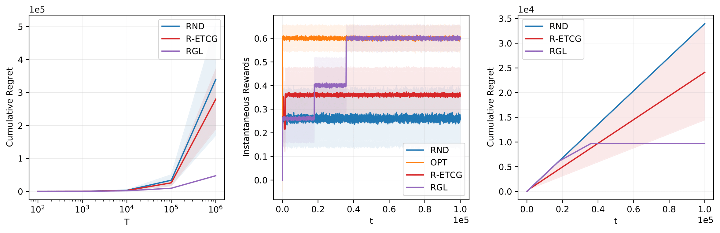
Figure 1: Comparison results for the non-monotone stochastic submodular reward function. From left to right, the plots show cumulative regret as a function of time step $T$, instantaneous rewards as a function of time step $t$, and cumulative regret as a function of time horizon $t$, respectively.

Figure 2: Comparison results for the non-monotone stochastic non-submodular reward function. From left to right, the plots show cumulative regret as a function of time step $T$, instantaneous rewards as a function of time step $t$, and cumulative regret as a function of time horizon $t$, respectively.

Theorem 1.

For the sequential decision making problem defined in Section 2 with $T\geq 2$, the expected cumulative $\frac{1}{2}$-regret of RGL is at most $\mathcal{O}(nT^{\frac{2}{3}}\log(T)^{\frac{1}{3}})$.

Proof.

We first condition the expected cumulative regret on the clean event.

$$\mathbb{E}(R(T)|\mathcal{E})$$ (25)

$$=\frac{1}{2}T\mathbb{E}[f\left(OPT\right)]-\sum_{t=1}^{T}\mathbb{E}[f\left(S_{t}\right)]$$

$$=\sum_{t=1}^{T}\left(\frac{1}{2}\mathbb{E}[f(OPT)]-\mathbb{E}[f\left(S_{t}\right)]\right)$$

$$=\sum_{i=1}^{n}\sum_{j=1}^{m}\biggr{[}\left(\frac{1}{2}\mathbb{E}[f(OPT)]-\mathbb{E}[f\left(X_{i-1}\right)]\right)$$

$$+\left(\frac{1}{2}\mathbb{E}[f(OPT)]-\mathbb{E}[f\left(X_{i-1}\cup\left\{u_{i}\right\}\right)]\right)$$

$$+\left(\frac{1}{2}\mathbb{E}[f(OPT)]-\mathbb{E}[f\left(Y_{i-1}\right)]\right)$$

$$+\left(\frac{1}{2}\mathbb{E}[f(OPT)]-\mathbb{E}[f\left(Y_{i-1}\setminus\left\{u_{i}\right\}\right)]\right)\biggr{]}$$

$$+\sum_{t=4nm+1}^{T}\left(\frac{1}{2}\mathbb{E}[f(OPT)]-\mathbb{E}[f\left(S_{t}\right)]\right).$$

We split the sum into two parts, the first accounting for cumulative regret incurred during the exploration phase and the second for the exploitation phase. During exploration, for each arm $u_{i}$ the agent plays four subsets, $X_{i}$, $Y_{i}$, $X_{i-1}\cup\left\{u_{i}\right\}$, and $Y_{i-1}\setminus\left\{u_{i}\right\}$, for $m$ times each. Hence, the agent explores for $4mn$ time steps. Since $f(\cdot)$ is bounded in $[0,1]$, for any subset $S_{t}$ played at time $t$ by the agent,

$$\frac{1}{2}\mathbb{E}[f\left(OPT\right)]-\mathbb{E}[f\left(S_{t}\right)]\leq\frac{1}{2}.\\$$ (26)

Substituting (26) in (25), we have

$$\mathbb{E}[R(T)\mid\mathcal{E}]$$

$$\leq 4nm\frac{1}{2}+\sum_{t=T_{n+1}}^{T}\left(\frac{1}{2}\mathbb{E}[f(OPT)]-\mathbb{E}[f\left(S_{t}\right)]\right)$$

$$=2nm+\sum_{t=T_{n+1}}^{T}\left(\frac{1}{2}\mathbb{E}[f(OPT)]-\mathbb{E}[f\left(X_{n}\right)]\right).$$

From Corollary 2, we have $\frac{1}{2}\mathbb{E}(f(OPT))-\mathbb{E}[f(X_{n})]\leq\frac{5}{2}n\,rad$. Thus,

$$\mathbb{E}[R(T)\mid\mathcal{E}] \leq 2nm+\sum_{t=T_{n+1}}^{T}\left(\frac{5}{2}n\,rad\right)$$

$$\leq 2nm+\frac{5}{2}Tn\,rad.$$

Since $rad=\sqrt{2\log(T)/m}$, we have

$$\mathbb{E}(R(T)\mid\mathcal{E}) \leq 2nm+\frac{5}{2}Tn\sqrt{2\frac{\log(T)}{m}}.$$

The above inequality is true for all $m$ strictly greater than zero. Hence, to find a tighter bound, we find $m^{*}$ that minimizes the left side. The exact minimizer is:

$$m^{\star}=\left(T\sqrt{\frac{25}{32}\log(T)}\right)^{2/3}.$$

Therefore, we choose $m=\lceil m^{\star}\rceil$.

$$\mathbb{E}(R(T)\mid\mathcal{E}) \leq 2n\lceil m^{\star}\rceil+\frac{5}{2}nT\sqrt{\frac{2\log(T)}{\lceil m^{\star}\rceil}}$$

$$\leq 2n\lceil m^{\star}\rceil+\frac{5}{2}nT\sqrt{\frac{2\log(T)}{m^{*}}}$$

For $T\geq 2$, $m^{\star}\geq\frac{1}{2}$ and thus $\lceil m^{\star}\rceil\leq 2m^{*}$. Thus, we have

$$\mathbb{E}(R(T)\mid\mathcal{E}) \leq 4nm^{\star}+\frac{5}{2}nT\sqrt{\frac{2\log(T)}{m^{*}}}$$

$$\leq\mathcal{O}(nT^{\frac{2}{3}}\log(T)^{\frac{1}{3}})$$

Under the bad event, i.e., the complement $\bar{\mathcal{E}}$ of the good event $\mathcal{E}$, given that the rewards are bounded in $[0,1]$, it can be easily seen that $\mathbb{E}(R(T)\mid\mathcal{\bar{E}})\leq T$. Moreover, by using Lemma 3 in Appendix B, the Hoeffding inequality (Hoeffding, 1994), we have $\mathbb{P}(\mathcal{\bar{E}})\leq\frac{8n}{T^{4}}$, see Lemma 4 in Appendix B. Therefore, we obtain $\mathbb{E}(R(T))\leq\mathcal{O}(nT^{\frac{2}{3}}\log(T)^{\frac{1}{3}}).$ ∎

Remark 3.

When the time horizon $T$ is not known, we can extend our result to an anytime algorithm using the geometric doubling trick. Essentially, we pick a geometric sequence $T_{i}=T_{0}2^{i}$ for $i\in\{1,2,\cdots\}$, where $T_{0}$ is a large enough number to let the algorithm initialize, and run RGL within time interval $T_{i+1}-T_{i}$ with a full restart, (Besson and Kaufmann, 2018). From Theorem 4 in the work of Besson and Kaufmann (2018), it follows that the regret bound conserves the original $T^{2/3}\log(T)^{1/3}$ dependence with only changes in constant factors.

5 Experiments

In this section, we empirically evaluate our RGL algorithm in non-monotone, submodular and non-submodular settings. For further experiments, we refer the reader to the linear reward minus cost experiment in Appendix D.1, and to the revenue maximization over social networks experiment in Appendix D.2.

We compare our method to the exact optimal solution and compute the empirical mean over different repetitions of the cumulative full regret instead of the cumulative $\frac{1}{2}$-regret, defined as follows,

$$\bar{\mathcal{R}}(T)=\frac{1}{rep}\sum_{n=1}^{rep}\sum_{t=1}^{T}(f\left(OPT\right)-f\left(S_{t}\right)).$$

We test the algorithms on a non-monotone stochastic submodular function of the chosen set $S$, defined as $f(S)=\min(\max(g(S)+\varepsilon,0),1)$, where $\varepsilon\sim\mathcal{N}(\mu,\sigma)$. In our experiments, we choose a non-monotone submodular example of $g(S)$, where $g(\left\{\right\})=0.2$, $g(\left\{1\right\})=0$, $g(\left\{2\right\})=0.6$, $g(\left\{1,2\right\})=0.2$. Note that $\mathbb{E}[f(S)]=g(S)$, and $g(S)$ is submodular.

In the second experiment, we choose a non-monotone non-submodular example of $g(S)$, where $g(\left\{\right\})=0.3$, $g(\left\{1\right\})=0$, $g(\left\{2\right\})=0.5$, $g(\left\{1,2\right\})=0.9$. Notice, that $\mathbb{E}[f(S)]=g(S)$, and $g(S)$ is not submodular.

We run our method for $T\in\left\{10^{2},10^{3},10^{4},10^{5},10^{6}\right\}$ time horizons. We assume $\varepsilon\sim\mathcal{N}(0,0.1)$. We average our experiments over $rep=20$ repetitions. We average the instantaneous rewards over a window of size 50.

We use the optimal solution, which is $\left\{2\right\}$ in the first experiment and $\left\{1,2\right\}$ in the second experiment, and run it in the online setting, where the optimal agent (OPT) only exploits the best set of arms throughout the time until $T$, see Algorithm 2. Moreover, we compare to random bandits (RND), see Algorithm 3, which at each time step plays a random subset of $\Omega$, where each arm is sampled independently with probability $\frac{1}{2}$. The random algorithm in the offline setting has $\frac{1}{4}$-approximation guarantee (Feige et al., 2011). Furthermore, we compare to one online monotone submodular maximization algorithm, ETCG, (Nie et al., 2022). Unfortunately, the online algorithms for monotone submodular maximization require an extra input, which is the cardinality $k$. Thus, we define R-ETCG, see Algorithm 4, which initially generates a random $k\sim\mathcal{U}(0,n)$, then finds the best $k$ arms.

From Fig. 1 for the sub-modular function case, it can be seen that RGL reaches the optimum. From Fig. 2, in the non-submodular case, it can be seen that RGL still reaches the optimum. In both experiments, RGL outperforms all the above-defined benchmarks. Even though the theory is not developed for non-submodular cases, the approach can still work well even in such cases. Further, the proposed algorithm outperforms R-ETCG, indicating that the algorithms for monotone functions cannot be directly applied to the non-monotone case.

Remark 4.

The cumulative regret upper bound dependence of $O(T^{2/3})$ is on the horizon $T$ (not time-step $t$) (see left sub-figures in all Figures, which have cumulative regret curves increasing in $T$). For a fixed time horizon T, RGL found the optimal set of arms, which makes its cumulative regret for a fixed time horizon T a constant w.r.t. time $t$ (right sub-figures for Fig. 1 and 2). Furthermore, the theoretical guarantees are for the worst-case scenario, i.e., the theory gives an upper bound on the regret, which for some instances, will be lower.

6 Conclusion

This paper proposes RGL, the first online stochastic non-monotone submodular maximization algorithm under full-bandit feedback, i.e. when the agent only receives the reward for a chosen set of arms and has no extra information about the individual arms. The proposed algorithm provably achieves a $\frac{1}{2}$-regret upper bound of $\tilde{\mathcal{O}}(nT^{\frac{2}{3}})$ for horizon $T$ and number of arms $n$. Moreover, the algorithm empirically outperforms the considered baselines under full-bandit feedback.

We note that the existing results for sub-modular bandits with full-bandit feedback also achieve $\tilde{\mathcal{O}}(T^{\frac{2}{3}})$ regret bound in the monotone function setup (Nie et al., 2022; Niazadeh et al., 2020). Further, the results for non-monotone function in adversarial setting is also $\tilde{\mathcal{O}}(T^{\frac{2}{3}})$ (Niazadeh et al., 2020). While a formal lower bound for this setup has not been studied, proving such a lower bound or improving the regret bounds in all these setups is an open problem.

7 Acknowledgement

This work was supported in part by the National Science Foundation under Grants 2149588 and 2149617.

Appendix A Motivating Examples for (Non-montone) Submodular Maximization

A.1 Data Summarization

As huge amount of data is generated daily, selecting a good representative subset of data points remains as a challenge. Often, the utility function capturing the coverage or diversity of a subset of the entire dataset satisfies submodularity (Mirzasoleiman et al., 2016). However, utility functions that accommodate diversity are not necessarily monotone as they penalize larger solutions (Tschiatschek et al., 2014; Dasgupta et al., 2013).

A.2 Feature Selection

One compelling use of non-monotone submodular maximization algorithms is modeling some learning problems such as feature selection (Das and Kempe, 2008; Khanna et al., 2017; Elenberg et al., 2018; Qian and Singer, 2019). Optimizing feature selection can be modeled as a non-monotone submodular maximization due to the possible overfitting to the training data (Fahrbach et al., 2018).

A.3 Recommender Systems

Recommending items with redundant information leads to diminishing returns on utility. This problem of sequentially recommending sets of items to users has been studied through the framework of contextual submodular combinatorial bandits (Qin and Zhu, 2013; Takemori et al., 2020). The optimization is not necessarily monotone as adding further recommendations might lead to a counter effect (Amanatidis et al., 2020).

A.4 Influence Maximization

One possible way to market a newly developed product can be done by selecting a set of highly influential people and hope they recommend it to their communities. A recent line of research has considered the problem as a multi-armed bandit problem (with extra feedback) without requiring the knowledge of the network and diffusion model (Lei et al., 2015; Wen et al., 2017; Vaswani et al., 2017; Li et al., 2020; Perrault et al., 2020). Most works consider that there is a fixed constraint on cardinality or budget. However, a revenue maximization model to maximize income from influence minus the costs is in general a non-monotone unconstrained submodular maximization problem (Lu and Lakshmanan, 2012).

Appendix B Additional Lemmas and Proofs

B.1 Probability of the Clean Event

Hoeffding’s inequality (Hoeffding, 1994) is a powerful technique for bounding probabilities of bounded random variables. We state the inequality, then we use it to show that $\mathcal{E}$ happens with high probability.

Lemma 3.

(Hoeffding’s inequality). Let $X_{1},X_{2},...,X_{n}$ be independent random variable bounded in $[0,1]$ and let $\bar{X}$ their empirical mean. Then we have for any $\varepsilon>0$,

$$\mathbb{P}(|\bar{X}-\mathbb{E}(X)|\geq\varepsilon)\leq 2\exp\left(-2n\varepsilon^{2}\right).$$

Lemma 4.

The probability of clean event $\mathcal{E}$ satisfies

$$\mathbb{P}(\mathcal{E})\geq 1-\frac{8n}{T^{4}}.$$ (27)

Proof.

Applying Lemma 3 to the empirical mean $\bar{f}\left(S\right)$ of $m$ rewards for action $S$ and choosing $\epsilon=\operatorname{rad}=$ $\sqrt{2\log(T)/m}$, we have

$$\mathbb{P}\left[\left|\bar{f}\left(S\right)-f\left(S\right)\right|\geq\operatorname{rad}\right] \leq 2\exp\left(-2m\operatorname{rad}^{2}\right)$$ (by Lemma 3)

$$=2\exp(-2m(2\log(T)/m))$$

$$=2\exp(-4\log(T))$$

$$=\frac{2}{T^{4}}.$$ (28)

For each arm $u_{i}$, the agent plays the following list of actions $\mathcal{S}_{i}=\left[X_{i-1},X_{i-1}\cup\left\{u_{i}\right\},Y_{i-1},Y_{i-1}\backslash\left\{u_{i}\right\}\right]$ exactly $m$ times, then computes marginal gain estimates. Thus, for any individual action $S\in\mathcal{S}_{i}$, we can bound the probability that its sample mean $\bar{f}\left(S\right)$ is within a specified confidence radius (complementary of the event above) as

$$\forall S\in\mathcal{S}_{i}\quad\mathbb{P}\left[\left|\bar{f}\left(S\right)-f\left(S\right)\right|<\operatorname{rad}\right] =1-\mathbb{P}\left[\left|\bar{f}\left(S\right)-f\left(S\right)\right|\geq\operatorname{rad}\right]$$

$$\geq 1-\frac{2}{T^{4}}.$$ (29)

We now focus on bounding $\mathbb{P}\left(\mathcal{E}_{i}\mid X_{i-1}=X,Y_{i-1}=Y\right)$. By conditioning on the sets decided in the previous phase, $X_{i-1}=X,Y_{i-1}=Y$, we know all the actions that will be played in the current phase $i$, i.e. $\mathcal{S}_{i}$. The rewards of all the actions are bounded in $[0,1]$ and are conditionally independent (given the corresponding action).

$$\mathbb{P}\left(\mathcal{E}_{i}\mid X_{i-1}=X,Y_{i-1}=Y\right) =\mathbb{P}\left(\bigcap_{S\in\mathcal{S}_{i}}\left\{\left|\bar{f}\left(S\right)-\mathbb{E}\left[f\left(S\right)\right]\right|<\operatorname{rad}\right\}\mid X_{i-1}=X,Y_{i-1}=Y\right)$$ (by (10))

$$=\prod_{S\in\mathcal{S}_{i}}\mathbb{P}\left(\left\{\left|\bar{f}\left(S\right)-f\left(S\right)\right|<\operatorname{rad}\right\}\mid X_{i-1}=X,Y_{i-1}=Y\right)$$ (rewards are independent when conditioned on actions)

$$\geq\left(1-\frac{2}{T^{4}}\right)^{\left|\mathcal{S}_{i}\right|}$$ (by (29))

$$=\left(1-\frac{2}{T^{4}}\right)^{4}$$ (30)

With this, we can then lower bound the probability of the clean event $\mathcal{E}$,

$$\mathbb{P}(\mathcal{E}) =\mathbb{P}\left(\mathcal{E}_{1}\cap\cdots\cap\mathcal{E}_{n}\right)$$ (by (11))

$$=\prod_{i=1}^{n}\mathbb{P}\left(\mathcal{E}_{i}\mid\mathcal{E}_{1},\ldots,\mathcal{E}_{i-1}\right)$$

$$=\prod_{i=1}^{n}\sum_{X,Y}\mathbb{P}\left(X_{i-1}=X,Y_{i-1}=Y,\mathcal{E}_{i}\mid\mathcal{E}_{1},\ldots,\mathcal{E}_{i-1}\right)$$ (law of total probability)

$$=\prod_{i=1}^{n}\sum_{X,Y}\mathbb{P}\left(X_{i-1}=X,Y_{i-1}=Y\mid\mathcal{E}_{1},\ldots,\mathcal{E}_{i-1}\right)\times\mathbb{P}\left(\mathcal{E}_{i}\mid X_{i-1}=X,Y_{i-1}=Y,\mathcal{E}_{1},\ldots,\mathcal{E}_{i-1}\right)$$

$$=\prod_{i=1}^{n}\sum_{X,Y}\mathbb{P}\left(X_{i-1}=X,Y_{i-1}=Y\mid\mathcal{E}_{1},\ldots,\mathcal{E}_{i-1}\right)\times\mathbb{P}\left(\mathcal{E}_{i}\mid X_{i-1}=X,Y_{i-1}=Y\right)$$

$$\geq\prod_{i=1}^{n}\sum_{X,Y}\mathbb{P}\left(X_{i-1}=X,Y_{i-1}=Y\mid\mathcal{E}_{1},\ldots,\mathcal{E}_{i-1}\right)\times\left(1-\frac{2}{T^{4}}\right)^{4}$$ (by (30))

$$=\prod_{i=1}^{n}\left(1-\frac{2}{T^{4}}\right)^{4}\sum_{X,Y}\mathbb{P}\left(X_{i-1}=X,Y_{i-1}=Y\mid\mathcal{E}_{1},\ldots,\mathcal{E}_{i-1}\right)$$

$$=\prod_{i=1}^{n}\left(1-\frac{2}{T^{4}}\right)^{4}$$

$$=\left(1-\frac{2}{T^{4}}\right)^{4n}$$

$$\geq\left(1-\frac{8n}{T^{4}}\right).$$ (Bernoulli’s inequality)

∎

B.2 Proof of Case 2 in Lemma 2.

It is sufficient to prove the inequality conditioned on any event of the form $X_{i-1}=S_{i-1}$ where $S_{i-1}\subseteq\left\{u_{1},...,u_{i-1}\right\}$, for which the probability $X_{i-1}=S_{i-1}$ is non-zero. The remainder of the proof assumes everything is conditioned on this event. The proof of Lemma 2 was divided in 4 cases in the text, where the detailed proof of three of them is provided in the main text. The proof of Case 2 is provided here for completeness.

Proof.

    Case 2 ($\bar{a}_{i}<0$ and $\bar{b}_{i}\geq 0$): In this case $\bar{a}_{i}\leq 0\Rightarrow a_{i}^{\prime}=0\Rightarrow\frac{b_{i}^{\prime}}{a_{i}^{\prime}+b_{i}^{\prime}}=1$. Thus, $X_{i}=X_{i-1}$ and $Y_{i}=Y_{i-1}\setminus\left\{u_{i}\right\}$. Since $Y_{i}=Y_{i-1}\setminus\left\{u_{i}\right\}$, we have

$$\mathbb{E}[b_{i}] =\mathbb{E}[f(Y_{i-1}\setminus\left\{u_{i}\right\})-f(Y_{i-1})]$$ (31)

$$=\mathbb{E}[f(Y_{i})-f(Y_{i-1})].$$

Since $X_{i}=X_{i-1}$, the relation (13) that we want to show reduces to,

$$\mathbb{E}[f(OPT_{i-1})-f(OPT_{i})]\leq\frac{1}{2}\mathbb{E}[f(Y_{i})-f(Y_{i-1})]+5rad.$$

Note that

$$OPT_{i}=\left(OPT\cup X_{i}\right)\cap Y_{i}=OPT_{i-1}\setminus\left\{u_{i}\right\}$$ (32)

If $u_{i}\notin OPT\Rightarrow OPT_{i}=OPT_{i-1}$. Thus,

$$\mathbb{E}[f(OPT_{i-1})-f(OPT_{i})] =0$$

$$\leq\frac{\bar{b}_{i}}{2}$$ (by case 2 condition)

$$\leq\frac{\mathbb{E}[b_{i}]}{2}+rad$$ (using concentration)

$$=\frac{1}{2}\mathbb{E}[f(Y_{i})-f(Y_{i-1})]+rad$$ (by (31))

$$\leq\frac{1}{2}\mathbb{E}[f(Y_{i})-f(Y_{i-1})]+5rad.$$

Now consider that $u_{i}\in OPT$. By definition of $OPT_{i-1}$, $X_{i-1}\subseteq OPT_{i-1}$. Since, $u_{i}\notin X_{i-1}$. Then, $X_{i-1}\subseteq OPT_{i-1}\setminus\left\{u_{i}\right\}$. Thus by submodularity in expectation,

$$\mathbb{E}[f\left(X_{i-1}\cup\left\{u_{i}\right\}\right)]-\mathbb{E}[f\left(X_{i-1}\right)]\geq\mathbb{E}[f(OPT_{i-1}\setminus\left\{u_{i}\right\})\cup\left\{u_{i}\right\}))]-\mathbb{E}[f(OPT_{i-1}\setminus\left\{u_{i}\right\})].$$ (33)

This allows us to finish the bound with

$$\mathbb{E}[f(OPT_{i-1})]-\mathbb{E}[f(OPT_{i})] =\mathbb{E}[f(OPT_{i-1})]-\mathbb{E}[f(OPT_{i-1}\setminus\left\{u_{i}\right\})]$$ (by (32))

$$=\mathbb{E}[f(OPT_{i-1}\setminus\left\{u_{i}\right\})\cup\left\{u_{i}\right\}))]-\mathbb{E}[f(OPT_{i-1}\setminus\left\{u_{i}\right\})]$$

$$\leq\mathbb{E}[f\left(X_{i-1}\cup\left\{u_{i}\right\}\right)]-\mathbb{E}[f\left(X_{i-1}\right)]$$ (by (33))

$$=\mathbb{E}[a_{i}] a_{i}$$ (by def. of )

$$\leq\bar{a}_{i}+2rad$$ (using concentration)

$$\leq\frac{\bar{b}_{i}}{2}+2rad$$ (condition for case 2)

$$\leq\frac{1}{2}\mathbb{E}[b_{i}]+3rad$$ (using concentration)

$$=\frac{1}{2}\mathbb{E}[f(Y_{i})-f(Y_{i-1})]+3rad$$ (by (31))

$$\leq\frac{1}{2}\mathbb{E}[f(Y_{i})-f(Y_{i-1})]+5rad.$$

∎

Appendix C Benchmarks

We now discuss benchmarks to assess the performance of our proposed algorithm.

C.1 Optimal Bandit

The optimal bandit (OPT) requires the optimal set of arms as an input, and it only exploits this set throughout the time until $T$, see Algorithm2. The optimal set should be known in advance, or found using some offline algorithm.

Algorithm 2 OPT

horizon $T$, solution $S^{\star}$

for step time $t\in\{1,\ldots,T\}$ do

     Play $S^{\star}$

end for

C.2 Random Bandit

The random bandits (RND), plays at each time step a random subset of $\Omega$, where each arm is sampled independently with probability $\frac{1}{2}$, see Algorithm 3. The random algorithm in the offline setting has $\frac{1}{4}$-approximation guarantee (Feige et al., 2011).

Algorithm 3 RND

Set of base arms $\Omega$, horizon $T$

$n\leftarrow|\Omega|$

for step time $t\in\{1,\ldots,T\}$ do

     $S^{(t)}\leftarrow\emptyset$

     for $i\in\{1,\ldots,n\}$ do

         with probability $\frac{1}{2}$ do

           $S^{(t)}\leftarrow S^{(t)}\cup\{u_{i}\}$

     end for

     Play $S^{(t)}$

end for

C.3 R-ETCG Bandit

Explore-then-commit greedy (ETCG) (Nie et al., 2022) is an online algorithm for monotone submodular maximization under full-bandit feedback, with proven guarantees in the monotone setting. The submodular monotone maximization, only makes sense when it is under constraint, otherwise the agent will pick all the arms as long as adding an arm is always beneficial. Therefore, the online algorithms for monotone submodular maximization require at least an extra input, such as the cardinality constraint $k$. Thus, to make applicable in our unconstrained non-monotone setting, we define random ETCG (R-ETCG), which initially generates a random cardinality budget $k\sim\mathcal{U}\left\{0,n\right\}$, then finds the best $k$ arms, see Algorithm 4.

Algorithm 4 R-ETCG

Set of base arms $\Omega$, horizon $T$

Initialize $S^{(0)}\leftarrow\emptyset,n\leftarrow|\Omega|,k\leftarrow\mathcal{U}\left\{0,n\right\}$

Initialize $m\leftarrow\left\lceil\left(\frac{T\sqrt{2\log(T)}}{n+2nk\sqrt{2\log(T)}}\right)^{2/3}\right\rceil$

for phase $i\in\{1,\ldots,k\}$ do

     for arm $a\in\Omega\backslash S^{(i-1)}$ do

         Play $S^{(i-1)}\cup\{a\}$ $m$ times

         Calculate the empirical mean $\bar{f}\left(S^{(i-1)}\cup\{a\}\right)$

     end for

     $a_{i}\leftarrow\arg\max_{a\in\Omega\backslash S^{(i-1)}}\bar{f}\left(S^{(i-1)}\cup\{a\}\right)$

     $S^{(i)}\leftarrow S^{(i-1)}\cup\left\{a_{i}\right\}$

end for

for remaining time do

     Play $S^{(k)}$

end for

Appendix D More Experimental Evaluations

In this section, we empirically evaluate our RGL algorithm in another non-monotone setting. We compare our method to the exact optimal solution and compute the empirical mean over different repetitions of the cumulative full regret instead of the cumulative $\frac{1}{2}$-regret, defined as follows,

$$\bar{\mathcal{R}}(T)=\frac{1}{rep}\sum_{n=1}^{rep}\sum_{t=1}^{T}(f\left(OPT\right)-f\left(S_{t}\right)).$$

We test for $n=8$ base arms, $T\in\left\{10^{2},10^{3},10^{4},10^{5},10^{6}\right\}$ time horizon. We average our experiments over $rep=9$ repetitions. We average the instantaneous rewards over a window of size 50.

D.1 Linear Reward Minus Cost

We test the algorithms on a non-monotone stochastic function of the chosen set $X$, defined as follows,

$$f(X)=\begin{cases}1,&\text{if }X=\{5,6,7,8\}\\ min(max(\sum_{a\in X}r(a)-\frac{|X|}{k^{\star}},0),1),&\text{ otherwise}\par\end{cases}$$

where $r(a)$ is the stochastic reward function of an individual arm where $\forall X,\forall a\in X,r(a)\in[0,1]$. In fact, we choose $r(a)\sim min(max(\mathcal{N}(\mu_{a},\sigma),0),1)$, where $\forall X,\forall a\in X,\mu_{a}\in[0,1]$.

We fix an oracle constant of the submodular function $k^{\star}=6$. We choose $\sigma=0.02$, and $\mu$ the vector of all the $\mu_{a}$s, such as $\mu$ values are arranged from 0 to 0.35 with a step of 0.05. It can be easily verified that the set $\{5,6,7,8\}$ is the optimal subset of arms.

From Fig. 3, it can be seen that our proposed algorithm RGL is the only one that reaches the optimum among the above defined benchmarks (middle plot) and it has the least cumulative regret in terms of time horizon T (left plot). In terms of time step t (right plot), similarly to RND, RGL starts by a higher cumulative reward compared to R-ETCG, which is explainable by the relatively long early exploration phase of RGL, however, in later time steps, RGL outperforms R-ETCG, by reaching less cumulative regret, by exploiting the optimum set of arms.

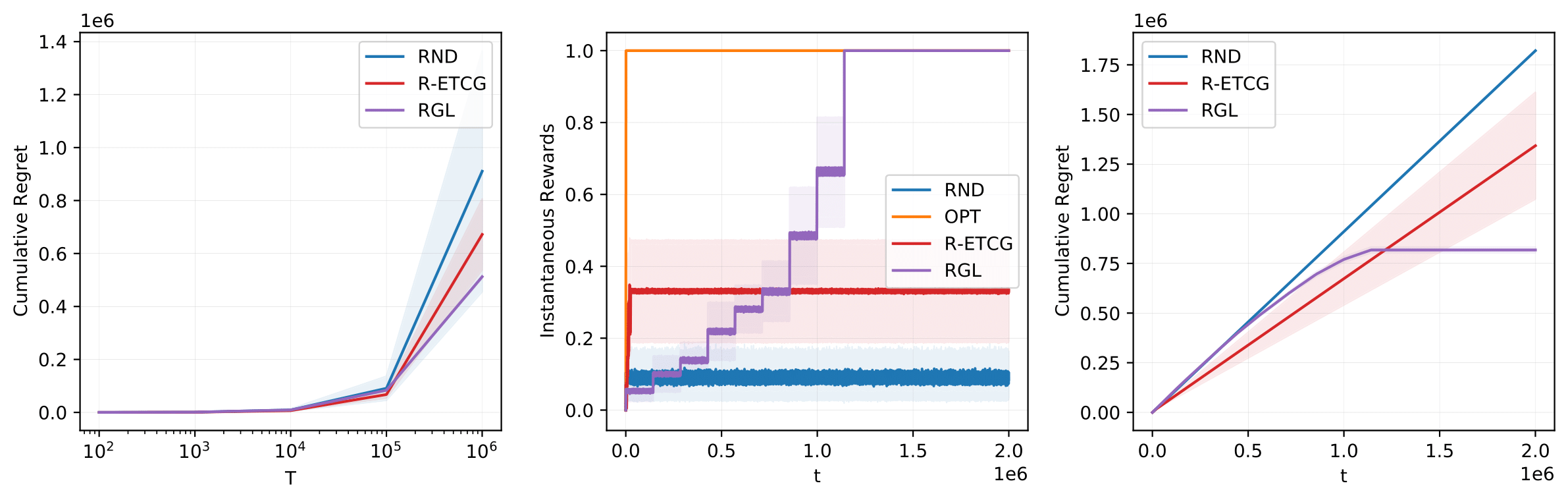
Figure 3: Comparison results for the non-monotone stochastic reward function. From left to right, the plots show cumulative regret as a function of time step $T$, instantaneous rewards as a function of time step $t$, and cumulative regret as a function of time horizon $t$, respectively.

D.2 Revenue Maximization over Social Networks

In several real-world scenarios, non-monotone objectives are more meaningful. For example, for revenue maximization over social networks, it is more meaningful to optimize the total revenue (influence minus costs; non-monotone) rather than the influence alone (monotone) with a budget as a constraint. Solutions to the latter will use all the budget, while the revenue-maximizing solution might use only a portion.

We test RGL on a non-monotone revenue maximization over social networks via influence maximization minus the costs. Influence maximization is indeed a submodular maximization problem which becomes non-monotone when we subtract the cost of adding nodes (Appendix A.4).

We use the Karate network, which includes $34$ nodes, with an oracle function $f$, where for a subset of nodes $S$,

$$f(S)=\mathcal{N}(\sum_{c\in\mathcal{C}}\max_{a\in S\cap c}d(a),\sigma)-\alpha|S|,$$

where $\mathcal{C}$ refers to the set of communities, $d(a)$ is the degree of node a, $\mathcal{N}$ is the normal distribution, and $\alpha$ is a positive constant which depends on the cost. As shown in Fig. 4, RGL outperforms all the other algorithms, as it has the lowest cumulative regret and almost reaches the optimal instantaneous rewards.

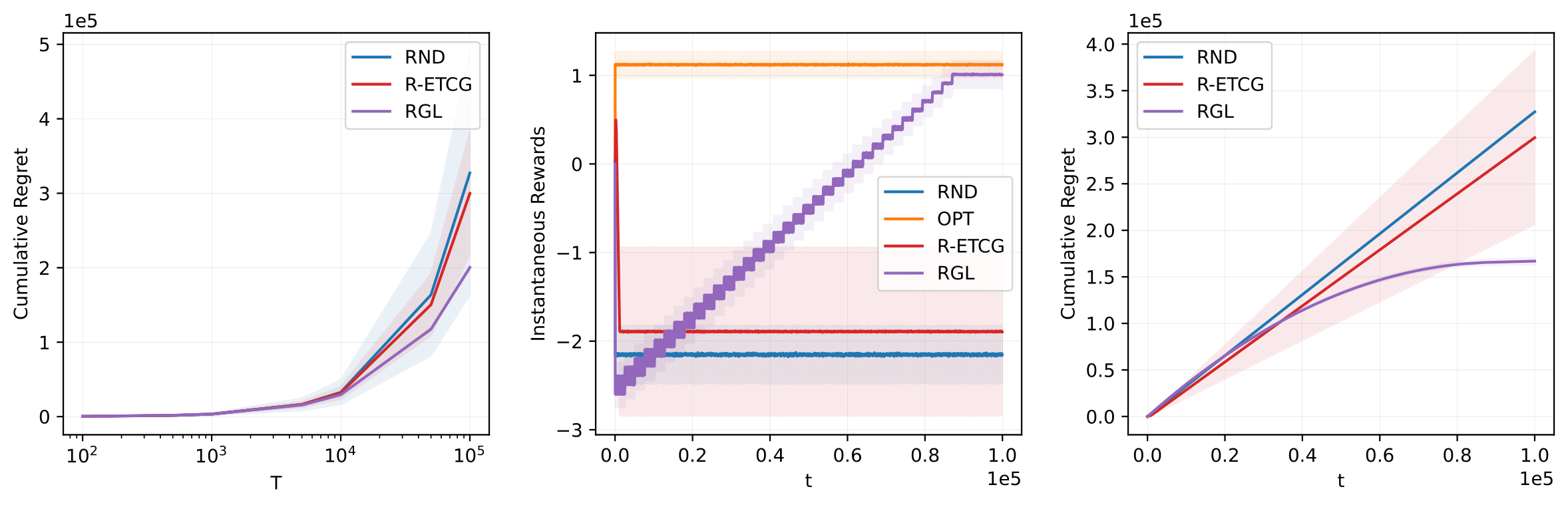
Figure 4: Revenue Maximization over Social Networks. From left to right, the plots show cumulative regret as a function of time step $T$, instantaneous rewards as a function of time step $t$, and cumulative regret as a function of time horizon $t$, respectively.

References

- Agrawal and Goyal (2012) Shipra Agrawal and Navin Goyal. Analysis of Thompson sampling for the multi-armed bandit problem. In Conference on learning theory, pages 39–1. JMLR Workshop and Conference Proceedings, 2012.
- Amanatidis et al. (2020) Georgios Amanatidis, Federico Fusco, Philip Lazos, Stefano Leonardi, and Rebecca Reiffenhäuser. Fast adaptive non-monotone submodular maximization subject to a knapsack constraint. Advances in Neural Information Processing Systems, 33:16903–16915, 2020.
- Auer (2002) Peter Auer. Using confidence bounds for exploitation-exploration trade-offs. Journal of Machine Learning Research, 3(Nov):397–422, 2002.
- Auer and Ortner (2010) Peter Auer and Ronald Ortner. UCB revisited: Improved regret bounds for the stochastic multi-armed bandit problem. Periodica Mathematica Hungarica, 61(1-2):55–65, 2010.
- Auer et al. (2002a) Peter Auer, Nicolo Cesa-Bianchi, and Paul Fischer. Finite-time analysis of the multiarmed bandit problem. Machine Learning, 47(2):235–256, 2002a.
- Auer et al. (2002b) Peter Auer, Nicolo Cesa-Bianchi, Yoav Freund, and Robert E Schapire. The nonstochastic multiarmed bandit problem. SIAM Journal on Computing, 32(1):48–77, 2002b.
- Besson and Kaufmann (2018) Lilian Besson and Emilie Kaufmann. What doubling tricks can and can’t do for multi-armed bandits. arXiv preprint arXiv:1803.06971, 2018.
- Buchbinder and Feldman (2018) Niv Buchbinder and Moran Feldman. Deterministic algorithms for submodular maximization problems. ACM Transactions on Algorithms (TALG), 14(3):1–20, 2018.
- Buchbinder et al. (2015) Niv Buchbinder, Moran Feldman, Joseph Seffi, and Roy Schwartz. A tight linear time (1/2)-approximation for unconstrained submodular maximization. SIAM Journal on Computing, 44(5):1384–1402, 2015.
- Chen et al. (2020) Lin Chen, Mingrui Zhang, Hamed Hassani, and Amin Karbasi. Black box submodular maximization: Discrete and continuous settings. In International Conference on Artificial Intelligence and Statistics, pages 1058–1070. PMLR, 2020.
- Das and Kempe (2008) Abhimanyu Das and David Kempe. Algorithms for subset selection in linear regression. In Proceedings of the fortieth annual ACM Symposium on Theory of Computing, pages 45–54, 2008.
- Dasgupta et al. (2013) Anirban Dasgupta, Ravi Kumar, and Sujith Ravi. Summarization through submodularity and dispersion. In Proceedings of the 51st Annual Meeting of the Association for Computational Linguistics (Volume 1: Long Papers), pages 1014–1022, Sofia, Bulgaria, August 2013. Association for Computational Linguistics.
- Edmonds (2003) Jack Edmonds. Submodular functions, matroids, and certain polyhedra. In Combinatorial Optimization—Eureka, You Shrink!, pages 11–26. Springer, 2003.
- Elenberg et al. (2018) Ethan R Elenberg, Rajiv Khanna, Alexandros G Dimakis, and Sahand Negahban. Restricted strong convexity implies weak submodularity. The Annals of Statistics, 46(6B):3539–3568, 2018.
- Fahrbach et al. (2018) Matthew Fahrbach, Vahab Mirrokni, and Morteza Zadimoghaddam. Non-monotone submodular maximization with nearly optimal adaptivity and query complexity. arXiv preprint arXiv:1808.06932, 2018.
- Feige (1998) Uriel Feige. A threshold of ln n for approximating set cover. Journal of the ACM (JACM), 45(4):634–652, 1998.
- Feige et al. (2011) Uriel Feige, Vahab S Mirrokni, and Jan Vondrák. Maximizing non-monotone submodular functions. SIAM Journal on Computing, 40(4):1133–1153, 2011.
- Goemans and Williamson (1995) Michel X Goemans and David P Williamson. Improved approximation algorithms for maximum cut and satisfiability problems using semidefinite programming. Journal of the ACM (JACM), 42(6):1115–1145, 1995.
- Gopalan et al. (2014) Aditya Gopalan, Shie Mannor, and Yishay Mansour. Thompson sampling for complex online problems. In Proceedings of the 31st International Conference on Machine Learning, volume 32 of Proceedings of Machine Learning Research, pages 100–108, Bejing, China, 22–24 Jun 2014. PMLR.
- Hoeffding (1994) Wassily Hoeffding. Probability inequalities for sums of bounded random variables. In The collected works of Wassily Hoeffding, pages 409–426. Springer, 1994.
- Iwata et al. (2001) Satoru Iwata, Lisa Fleischer, and Satoru Fujishige. A combinatorial strongly polynomial algorithm for minimizing submodular functions. Journal of the ACM (JACM), 48(4):761–777, 2001.
- Khanna et al. (2017) Rajiv Khanna, Ethan Elenberg, Alex Dimakis, Sahand Negahban, and Joydeep Ghosh. Scalable greedy feature selection via weak submodularity. In Artificial Intelligence and Statistics, pages 1560–1568. PMLR, 2017.
- Lattimore and Szepesvári (2020) Tor Lattimore and Csaba Szepesvári. Bandit algorithms. Cambridge University Press, 2020.
- Lei et al. (2015) Siyu Lei, Silviu Maniu, Luyi Mo, Reynold Cheng, and Pierre Senellart. Online influence maximization. In Proceedings of the 21th ACM SIGKDD International Conference on Knowledge Discovery and Data Mining, pages 645–654, 2015.
- Li et al. (2020) Shuai Li, Fang Kong, Kejie Tang, Qizhi Li, and Wei Chen. Online influence maximization under linear threshold model. Advances in Neural Information Processing Systems, 33:1192–1204, 2020.
- Lu and Lakshmanan (2012) Wei Lu and Laks VS Lakshmanan. Profit maximization over social networks. In 2012 IEEE 12th International Conference on Data Mining, pages 479–488. IEEE, 2012.
- Mirzasoleiman et al. (2016) Baharan Mirzasoleiman, Ashwinkumar Badanidiyuru, and Amin Karbasi. Fast constrained submodular maximization: Personalized data summarization. In International Conference on Machine Learning, pages 1358–1367. PMLR, 2016.
- Niazadeh et al. (2020) Rad Niazadeh, Negin Golrezaei, Joshua Wang, Fransisca Susan, and Ashwinkumar Badanidiyuru. Online learning via offline greedy: Applications in market design and optimization. EC 2021, Management Science Journal, 2020.
- Nie et al. (2022) Guanyu Nie, Mridul Agarwal, Abhishek Kumar Umrawal, Vaneet Aggarwal, and Christopher John Quinn. An explore-then-commit algorithm for submodular maximization under full-bandit feedback. In The 38th Conference on Uncertainty in Artificial Intelligence, 2022.
- Perrault et al. (2020) Pierre Perrault, Jennifer Healey, Zheng Wen, and Michal Valko. Budgeted online influence maximization. In International Conference on Machine Learning, pages 7620–7631. PMLR, 2020.
- Qian and Singer (2019) Sharon Qian and Yaron Singer. Fast parallel algorithms for statistical subset selection problems. Advances in Neural Information Processing Systems, 32, 2019.
- Qin and Zhu (2013) Lijing Qin and Xiaoyan Zhu. Promoting diversity in recommendation by entropy regularizer. In Twenty-Third International Joint Conference on Artificial Intelligence. Citeseer, 2013.
- Robbins (1952) Herbert Robbins. Some aspects of the sequential design of experiments. Bulletin of the American Mathematical Society, 58(5):527–535, 1952.
- Roughgarden and Wang (2018) Tim Roughgarden and Joshua R. Wang. An optimal learning algorithm for online unconstrained submodular maximization. In Proceedings of the 31st Conference On Learning Theory, pages 1307–1325, 2018.
- Takemori et al. (2020) Sho Takemori, Masahiro Sato, Takashi Sonoda, Janmajay Singh, and Tomoko Ohkuma. Submodular bandit problem under multiple constraints. In Conference on Uncertainty in Artificial Intelligence, pages 191–200. PMLR, 2020.
- Thompson (1933) William R Thompson. On the likelihood that one unknown probability exceeds another in view of the evidence of two samples. Biometrika, 25(3-4):285–294, 1933.
- Tschiatschek et al. (2014) Sebastian Tschiatschek, Rishabh K Iyer, Haochen Wei, and Jeff A Bilmes. Learning mixtures of submodular functions for image collection summarization. Advances in Neural Information Processing Systems, 27, 2014.
- Vaswani et al. (2017) Sharan Vaswani, Branislav Kveton, Zheng Wen, Mohammad Ghavamzadeh, Laks VS Lakshmanan, and Mark Schmidt. Model-independent online learning for influence maximization. In International Conference on Machine Learning, pages 3530–3539. PMLR, 2017.
- Wen et al. (2017) Zheng Wen, Branislav Kveton, Michal Valko, and Sharan Vaswani. Online influence maximization under independent cascade model with semi-bandit feedback. Advances in Neural Information Processing Systems, 30, 2017.