Geometric Deep Learning for Autonomous Driving: Unlocking the Power of Graph Neural Networks With CommonRoad-Geometric

Abstract

Heterogeneous graphs offer powerful data representations for traffic, given their ability to model the complex interaction effects among a varying number of traffic participants and the underlying road infrastructure. With the recent advent of graph neural networks (GNNs) as the accompanying deep learning framework, the graph structure can be efficiently leveraged for various machine learning applications such as trajectory prediction. As a first of its kind, our proposed Python framework offers an easy-to-use and fully customizable data processing pipeline to extract standardized graph datasets from traffic scenarios. Providing a platform for GNN-based autonomous driving research, it improves comparability between approaches and allows researchers to focus on model implementation instead of dataset curation.

I Introduction

\begin{overpic}[trim=401.49998pt 265.99374pt 501.87498pt 100.37498pt,clip,width=433.62pt]{figures/crgeo_highlevel_final2.pdf} \@@toccaption{{\lx@tag[ ]{{1}}{Our package serves as a bridge from CommonRoad to PyTorch-Geometric. The abbreviated graph labels refer to the heterogeneous node and edge entities of our unified traffic graph structure covered in~{}\lx@cref{creftype~refnum}{section:graph-representation}. }}}\@@caption{{\lx@tag[: ]{{\small Figure 1}}{\small Our package serves as a bridge from CommonRoad to PyTorch-Geometric. The abbreviated graph labels refer to the heterogeneous node and edge entities of our unified traffic graph structure covered in~{}\lx@cref{creftype~refnum}{section:graph-representation}. }}}\put(70.0,23.0){{v2l}} \put(87.5,20.0){{v2v}} \put(87.5,23.0){{l2l}} \put(76.5,28.0){{v}} \put(92.7,14.9){{l}} \end{overpic}

Machine learning agents require an accurate understanding of the surrounding traffic context to make safe and effective decisions [Lefevre2014]. This calls for a descriptive representation not only of the various entities within the traffic environment, but also their complex spatial and temporal relationships. When restricted to a fixed-size feature space—a prerequisite for classical neural networks—this is a particularly challenging prospect given the inherent complexity and variability in road geometries and traffic situations.

An alternative approach is to model the environment state in the form of a heterogeneous graph, encompassing both the road network topology and the traffic participants present in it. This structured representation allows us to capture a wide range of road networks and traffic scenarios with a variable number of discrete elements. Additionally, it enables the explicit modeling of pairwise relationships or interactions between entities through edge connections. Graph neural networks (GNNs) have recently emerged as the principal deep learning framework for processing graph data [bronstein_2017, chami_machine_2021, hetero_gnn_wang_2019, battaglia_2018]. By using GNNs, the graph topology can be exploited as a relational inductive bias [battaglia_2018] during training, aiding generalization.

I-A Related work

Graph-structured representations of traffic proposed in existing works differ based on the objectives of the learning task. In [jepsen_2019], the authors let nodes represent individual road segments with edges forming the overarching road network topology for driving speed estimation and road network classification. Alternatively, [diehl_2019] and [jeon2020_scalenet] present graph-based traffic forecasting approaches in which nodes are used to model traffic participants and edges are used to capture vehicle interactions. Similarly, [huegle_dynamic_2019] and [hart_graph_2020] adopt vehicle-to-vehicle GNNs as policy networks for reinforcement learning agents. Additionally considering the temporal dimension, [liGRIPGraphbasedInteractionaware2019] employs a spatiotemporal vehicle graph for capturing time-dependent features. Finally, recent works [liang_lane_graph_2020, zeng_lanercnn_2021, zhao2020tnt, kim_lapred_2021, zhang2021trajectory, janjo2021starnet, ngiam2021scene, gilles2021gohome, mo_2022_edge_enhanced] incorporate both vehicle and map nodes by modelling the environment as a heterogeneous graph, including both inter-vehicle as well as vehicle-road interaction effects.

I-B Motivation and contributions

Despite the vast research interest, there is no software framework that offers an interface for extracting custom graph datasets from traffic scenarios. Although there are plenty of autonomous driving datasets, e.g.  [krajewskiHighDDatasetDrone2018, interactiondataset, caesar_nuplan_2022], researchers have to write considerable amounts of ad-hoc, error-prone conversion code to use them as inputs for GNN models. As evident by the success in other application domains such as bioinformatics and social networks [morris_2020_tudataset, leskovec_2024_snapsets], standardized graph datasets would enable autonomous driving researchers to streamline their experiments and ensure comparability and repeatability of their results.

To fill this gap, we propose CommonRoad-Geometric (cr-geo): a Python library designed to facilitate the extraction of graph data from recorded or simulated traffic scenarios. Our framework extends the CommonRoad [commonroad_paper] software platform and uses its standardized interface for a high-level representation of the traffic environment. As illustrated by LABEL:fig:crgeo_highlevel, our framework unifies the traffic scene into a single graph entity, encompassing both the traffic participants and the underlying road map. The extracted graph representations are based on the HeteroData class offered by PyTorch-Geometric [pygeo], a popular PyTorch [pytorch] extension for deep learning on graph-structured data.

Our paper offers the following contributions:

• we introduce a heterogeneous graph structure for map-aware traffic representations tailored to GNN applications;

• we present and outline the software architecture of CommonRoad-Geometric (cr-geo), which offers a bridge from the well-established CommonRoad scenario format to PyTorch-Geometric (PyG);

• as a concrete example of the wide range of GNN-based applications facilitated by cr-geo, we train a spatiotemporal trajectory prediction model on a real-world graph dataset extracted from NuPlan [caesar_nuplan_2022].

II Background

We first provide some background on heterogeneous graphs and the description of scenarios in CommonRoad.

II-1 Heterogeneous graphs

A directed heterogeneous graph ${\mathcal{G}=(\mathcal{V},\mathcal{E},\mathcal{A},\mathcal{R},\mathcal{X}_{\mathcal{V}},\mathcal{X}_{\mathcal{E}})}$ is defined as a tuple of a set of nodes $\mathcal{V}$, edges $\mathcal{E}$, node types $\mathcal{A}$, edge types $\mathcal{R}$, and corresponding node and edge features $\mathcal{X}_{\mathcal{V}}$ and $\mathcal{X}_{\mathcal{E}}$ [jizhou_2013_heterograph]. Edges are defined as a 3-tuple ${\mathcal{E}\subset\mathcal{V}\times\mathcal{R}\times\mathcal{V}}$. Further, each node ${v\in\mathcal{V}}$ is assigned a node type via the mapping ${\tau_{V}(v):\mathcal{V}\rightarrow\mathcal{A}}$. Analogously, edges ${e\in\mathcal{E}}$ are associated with an edge type ${\tau_{\mathcal{E}}(e):\mathcal{E}\rightarrow\mathcal{R}}$. Finally, $\mathcal{X}_{\mathcal{V}}$ and $\mathcal{X}_{\mathcal{E}}$ contain the feature vectors, which we denote as ${\bm{\mathbf{x}}_{v}\in\mathbb{R}^{D_{\mathcal{V}}}}$ for node features and ${\bm{\mathbf{x}}_{e}\in\mathbb{R}^{D_{\mathcal{E}}}}$ for edge features. Fig. 2 illustrates graph features on the node and edge level.

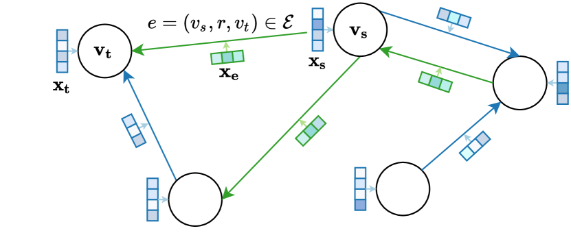
Figure 2: Illustration of a simple graph structure. Edge types are represented as different colors. Colored squares represent features vectors for nodes (e.g., vehicle speed) and edges (e.g., distance between vehicles).

II-2 CommonRoad

A CommonRoad scenario contains a set $\mathcal{V}^{cr}$ of dynamic obstacles. For a vehicle $V\in\mathcal{V}^{cr}$ of rectangular shape $(l_{V},w_{V})$, we represent its time-dependent state by its x-y center position $\bm{\mathbf{p}}_{V}$, its orientation $\theta_{V}$, as well as their time derivatives in the scenario coordinate frame.

Further, the map-related information of a scenario is described by its lanelet network, containing a set $\mathcal{L}^{cr}$ of atomic lanelets and their longitudinal and lateral adjacency relations [bender_lanelets]. Lanelets are geometrically defined by their boundary polylines. For a lanelet $L\in\mathcal{L}^{cr}$, we denote its left and right boundary polylines as $S_{L,l}$ and $S_{L,r}$, respectively. Further, we denote the center polyline as $S_{L,c}$. Each polyline is made up of a sequence of $N_{L}$ waypoints in the scenario coordinate frame. Using the notation $\langle\square_{i}\rangle_{i\in 1,...,N}$ to define a sequence of values of length $N$, we let the polylines be denoted as ${S_{L,l}=\langle\vec{s}_{l,i}\rangle_{i\in 1,...,N_{L}}}$, ${S_{L,r}=\langle\vec{s}_{r,i}\rangle_{i\in 1,...,N_{L}}}$, and ${S_{L,c}=\langle\vec{s}_{c,i}\rangle_{i\in 1,...,N_{L}}}$. With $\lVert\rVert_{2}$ denoting the L2-norm, we further define the lanelet length as

$$\lVert L\rVert_{2} =\sum_{i=1}^{N_{L}-1}\sqrt{\lVert\vec{s}_{c,i+1}-\vec{s}_{c,i}\rVert_{2}},$$ (1)

III Overview

In the following subsections, we define the structure of our traffic graph and outline the software architecture of our framework.

III-A Traffic graph structure

Extending PyG’s HeteroData, cr-geo’s CommonRoadData class represents a heterogeneous traffic graph encapsulating nodes of both the vehicle ( V ) and lanelet ( L ) node type, as well as the structural metadata for the specific graph instance. Formally, we have that ${\mathcal{A}=\{\text{\scalebox{0.85}[0.74]{V}},\text{\scalebox{0.85}[0.74]{L}}\}}$ and ${\mathcal{R}=\{\text{\scalebox{0.85}[0.74]{L}\scalebox{1.12}[1.0]{2}\scalebox{0.85}[0.74]{L}},\text{\scalebox{0.85}[0.74]{V}\scalebox{1.12}[1.0]{2}\scalebox{0.85}[0.74]{V}},\text{\scalebox{0.85}[0.74]{V}\scalebox{1.12}[1.0]{2}\scalebox{0.85}[0.74]{L}},\text{\scalebox{0.85}[0.74]{L}\scalebox{1.12}[1.0]{2}\scalebox{0.85}[0.74]{V}}\}}$.

In order to capture temporal vehicle interactions with GNN-based message-passing schemes, we further extend the CommonRoadData class by the time dimension with CommonRoadTemporalData, where $\mathcal{R}$ is augmented by the temporal V T V edge type. The resulting temporal graph [jain_2016_spatio_temporal_rnn], as shown in LABEL:fig:vtv_edges, intrinsically encodes the temporal dimension by unrolling the traffic graph over time. Vehicle nodes are repeated to capture vehicle states at past timesteps, and temporal edges encode the time difference between them.

\begin{overpic}[trim=250.93748pt 100.37498pt 200.74998pt 200.74998pt,clip,width=433.62pt,tics=10]{figures/temporal_edges_23.pdf} \@@toccaption{{\lx@tag[ ]{{3}}{Visualization of Voronoi-based {v2v} and causal {vtv} edges for a highway scenario. Opaque colors denote the most recent edges while more transparent shades represent older ones.}}}\@@caption{{\lx@tag[: ]{{\small Figure 3}}{\small Visualization of Voronoi-based {v2v} and causal {vtv} edges for a highway scenario. Opaque colors denote the most recent edges while more transparent shades represent older ones.}}}\put(41.0,10.5){\footnotesize$t-4$} \put(46.2,11.4){\rotatebox{9.0}{\ldots}} \put(51.2,11.9){\footnotesize$t$} \put(1.8,8.5){\footnotesize$t$} \put(52.7,1.0){\rotatebox{9.0}{Direction of traffic}} \put(1.8,15.0){\footnotesize$t-1$} \put(1.8,22.0){\footnotesize$t-2$} \put(38.0,23.0){\color[rgb]{0.0,0.7,0.1}{v2v}} \put(29.0,25.0){\rotatebox{-45.0}{\color[rgb]{0,0,1}{vtv}}} \put(0.5,7.5){\color[rgb]{0,0,0}\vector(0,1){31.0}} \put(1.8,29.0){\footnotesize$t-3$} \put(1.8,35.5){\footnotesize$t-4$} \end{overpic}

The heterogeneous structure of our graphical data representation is summarized in Tab. II and outlined in the following paragraphs:

III-A1 Lanelet nodes $(\mathcal{V}_{L})$

Lanelet nodes map to the lanelets in $\mathcal{L}^{cr}$, with each lanelet $L$ being represented as a graph node. The corresponding node features encode the geometric properties of the respective lanelets. Using the general notation ${}^{L}\square$, we denote the lanelet-local transformed polyline coordinates as ${}^{L}S_{L,l}$, ${}^{L}S_{L,c}$, and ${}^{L}S_{L,r}$. Here, the vertex coordinates are transformed to the lanelet-local coordinate frame according to its origin position ${\bm{\mathbf{p}}_{L}=\vec{s}_{c,1}}$ and its orientation ${\theta_{L}=\operatorname{atan2}{\left(\nicefrac{{\vec{s}_{c,2}}}{{\vec{s}_{c,1}}}\right)}}$. In the following, we also let the function interpretations $\tilde{S}_{L,\square}(\cdot)$ and $\tilde{\theta}_{L}(\cdot)$ be defined via orthogonal projections onto the polylines, returning the position and orientation at a given arclength, respectively.

III-A2 Lanelet-to-lanelet edges $(\mathcal{E}_{\textsc{l2l}})$

Lanelet-to-lanelet edges characterize the lanelet network topology and encode the spatial relationship between adjacent lanelets. As illustrated by Fig. 4, we explicitly differentiate between the heterogeneous l2l adjacency types $\mathcal{R}_{\textsc{l2l}}$ listed in Tab. I via the edge feature $\tau_{\mathcal{E}}$. For an edge from $L$ to $L^{{}^{\prime}}$, we also include their centerline arclength distance at the point of intersection as edge features, which we denote by $s_{L}$ and $s_{L^{{}^{\prime}}}$. This is highlighted in LABEL:fig:l2l_intersection for two conflicting lanelets.

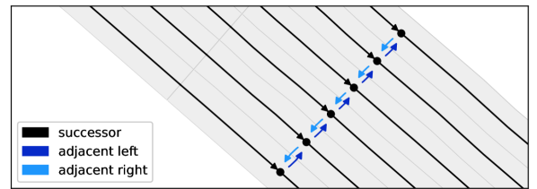
((a)) Highway scenario containing five parallel lanelets.

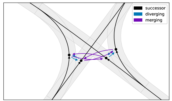
((b)) Intersection scenario highlighting merging and diverging lanelets.

\begin{overpic}[trim=63.03549pt 100.37498pt 50.38824pt 100.37498pt,clip,width=433.62pt]{figures/l2l_conversion_6-eps-converted-to.pdf} \par\par\put(54.0,30.3){ \leavevmode\hbox to60.25pt{\vbox to3.2pt{\text{[drawing]}}}} \put(79.6,29.6){\footnotesize{$s_{L}$, $s_{L^{{}^{\prime}}}$}} \put(47.0,15.0){\color[rgb]{0.97,0.15,0.52}\scriptsize{ $L\rightarrow L^{{}^{\prime}}$}} \par\put(60.3,24.0){\footnotesize{ $L^{{}^{\prime}}$}} \put(39.5,21.5){\footnotesize{ $L$}} \par\par\end{overpic}

((c))

Figure 4: Lanelet graphs highlighting l2l adjacency types.

TABLE I: l2l adjacency types for edges $L\rightarrow L^{\prime}$. The considered adjacency types can be individually selected at the user’s preference.

Type	Interpretation
predecessor	$L$ continues the driving corridor of $L^{\prime}$
successor	$L^{\prime}$ continues the driving corridor of $L$
adjacent left	$L$ is left-adjacent to $L^{\prime}$
adjacent right	$L$ is right-adjacent to $L^{\prime}$
merging	$L$ and $L^{\prime}$ share a common successor (symmetric)
diverging	$L$ and $L^{\prime}$ share a common predecessor (symmetric)
conflicting	$L$ and $L^{\prime}$ cross each other (symmetric)

III-A3 Vehicle nodes $(\mathcal{V}_{V})$

Vehicle nodes are inserted according to the states of the currently present vehicles and identified by their CommonRoad IDs. As shown in LABEL:fig:vtv_edges, CommonRoadTemporalData additionally includes past vehicle states in the graph representation: here, a vehicle’s state history is captured by time-attributed (but otherwise identical) vehicles nodes inserted at each timestep.

III-A4 Vehicle-to-vehicle edges $(\mathcal{E}_{\textsc{v2v}})$

Vehicle-to-vehicle edges capture the interaction between vehicles at each timestep. The relative pose of connected vehicles is encoded as edge features according to the vehicle-local coordinate frame originating at the center of the source vehicle. Users can provide a specific implementation of our V 2 V edge drawer protocol to encode which V 2 V relations are relevant for their task. Our framework offers developers a set of standard edge drawer implementations, two of which are depicted in Fig. 5.

((a)) VoronoiEdgeDrawer inserts edges according to a Delaunay triangulation.

((b)) KNearestEdgeDrawer connects the $k$ closest vehicles (here with $k=3$).

Figure 5: v2v edges drawn by two different implementations.

TABLE II: Overview of node ($\mathcal{X}_{\mathcal{V}}$) and edge ($\mathcal{X}_{\mathcal{E}}$) features.

Type	Feature	Notation	Unit	Size
$\underset{\underset{(L)}{}}{\textsc{l}}$	Position	$\bm{\mathbf{p}}_{L}$	$\text{\,}\mathrm{m}\text{/}$	2
	Length	$\lVert L\rVert_{2}$	$\text{\,}\mathrm{m}\text{/}$	$1$
	Orientation	$\theta_{L}$	$\text{\,}\mathrm{r}\mathrm{a}\mathrm{d}$	$1$
	Left vertices	${}^{L}V_{l}$	$\text{\,}\mathrm{m}\text{/}$	$2\cdot N_{L}$
	Right vertices	${}^{L}V_{r}$	$\text{\,}\mathrm{m}\text{/}$	$2\cdot N_{L}$
	Custom feature vector	$\bm{\mathbf{x}}_{v}^{(\textsc{l})}$	—
$\underset{\underset{(V)}{}}{\textsc{v}}$	Position	$\bm{\mathbf{p}}_{V}$	$\text{\,}\mathrm{m}\text{/}$	2
	Orientation	$\theta_{V}$	$\text{\,}\mathrm{r}\mathrm{a}\mathrm{d}$	$1$
	Yaw-rate	$\dot{\theta}_{V}$	$\text{\,}\mathrm{r}\mathrm{a}\mathrm{d}\mathrm{/}\mathrm{s}$	$1$
	Velocity	$\dot{\bm{\mathbf{p}}}_{V}$	$\text{\,}\mathrm{m}\mathrm{/}\mathrm{s}$	$2$
	Acceleration	$\bm{\mathbf{\ddot{p}}}_{V}$	$\text{\,}\mathrm{m}\mathrm{/}\mathrm{s}^{2}$	$2$
	Vehicle width	$w_{V}$	$\text{\,}\mathrm{m}\text{/}$	$1$
	Vehicle length	$l_{V}$	$\text{\,}\mathrm{m}\text{/}$	$1$
	Custom feature vector	$\bm{\mathbf{x}}_{v}^{(\textsc{v})}$	—
$\underset{\underset{(L\rightarrow L^{{}^{\prime}})}{}}{\textsc{l2l}}$	Distancea	$\lVert\bm{\mathbf{p}}_{L^{{}^{\prime}}}-\bm{\mathbf{p}}_{L}\rVert_{2}$	$\text{\,}\mathrm{m}\text{/}$	1
	Relative positiona	${}^{L}\bm{\mathbf{p}}_{L^{{}^{\prime}}}$	$\text{\,}\mathrm{m}\text{/}$	$2$
	Relative orientationa	$\theta_{L^{{}^{\prime}}}-\theta_{L}$	$\text{\,}\mathrm{r}\mathrm{a}\mathrm{d}$	$1$
	Intersection (source)	$s_{L}$	$\text{\,}\mathrm{m}\text{/}$	$1$
	Intersection (target)	$s_{L^{{}^{\prime}}}$	$\text{\,}\mathrm{m}\text{/}$	$1$
	Adjacency type	$\tau_{\mathcal{E}}$	—	$1$
	Custom feature vector	$\bm{\mathbf{x}}_{e}^{(\textsc{l2l})}$	—
$\underset{\underset{(V\rightarrow V^{{}^{\prime}})}{}}{\textsc{v2v}}$	Distance	$\lVert\bm{\mathbf{p}}_{V^{{}^{\prime}}}-\bm{\mathbf{p}}_{V}\rVert_{2}$	$\text{\,}\mathrm{m}\text{/}$	1
	Relative position	${}^{V}\bm{\mathbf{p}}_{V^{{}^{\prime}}}$	$\text{\,}\mathrm{m}\text{/}$	2
	Relative orientation	$\theta_{V^{{}^{\prime}}}-\theta_{V}$	$\text{\,}\mathrm{r}\mathrm{a}\mathrm{d}$	1
	Relative velocity	${}^{V}\dot{\bm{\mathbf{p}}}_{V^{{}^{\prime}}}-^{V}\!\dot{\bm{\mathbf{p}}}_{V}$	$\text{\,}\mathrm{m}\mathrm{/}\mathrm{s}$	$2$
	Relative acceleration	${}^{V}\ddot{\bm{\mathbf{p}}}_{V^{{}^{\prime}}}-^{V}\!\ddot{\bm{\mathbf{p}}}_{V}$	$\text{\,}\mathrm{m}\mathrm{/}\mathrm{s}^{2}$	$2$
	Custom feature vector	$\bm{\mathbf{x}}_{e}^{(\textsc{v2v})}$	—
vtvb	V 2 V features	.4pt " .4pt	.4pt " .4pt	.4pt " .4pt
	Time delta	$\Delta t_{e}$	$\text{\,}\mathrm{s}\text{/}$	$1$
	Custom feature vector	$\bm{\mathbf{x}}_{e}^{(\textsc{vtv})}$	—
$\underset{\underset{(V\rightarrow L)}{}}{\textsc{v2l}}$	Left distance	$d_{V,l}^{L}$	$\text{\,}\mathrm{m}\text{/}$	1
	Right distance	$d_{V,r}^{L}$	$\text{\,}\mathrm{m}\text{/}$	1
	Lateral offset	$d_{V,e}^{L}$	$\text{\,}\mathrm{m}\text{/}$	1
	Heading error	$\theta_{V,e}^{L}$	$\text{\,}\mathrm{r}\mathrm{a}\mathrm{d}$	$1$
	Projected arclength	$s_{V}^{L}$	$\text{\,}\mathrm{m}\text{/}$	$1$
	Normalized arclength	$\nicefrac{{s_{V}^{L}}}{{\lVert L\rVert_{2}}}$	—	$1$
	Custom feature vector	$\bm{\mathbf{x}}_{e}^{(\textsc{v2l})}$	—

^ameasured between the respective lanelet coordinate frames.
^bonly relevant for CommonRoadTemporalData.

III-A5 Vehicle-to-lanelet edges $(\mathcal{E}_{\textsc{v2l}})$

Vehicle-to-lanelet edges relate vehicles to the underlying road infrastructure. Our framework offers two assignment strategies for drawing the edges:

1. Center: Each vehicle is connected to all lanelets that contain the vehicle center point.

2. Shape: Each vehicle is connected to all lanelets that intersect with the vehicle shape. This constitutes a superset of the edges drawn by the Center strategy.

The associated edge features describe the relative pose of the vehicle with respect to the curvilinear lanelet coordinate frame [hery_2017_curvilinear]. For a given edge from vehicle $V$ to lanelet $L$, we denote the orthogonal distance from the lanelet’s left and right boundaries to the vehicle center as

$$d_{V,l}^{L} =\lVert\tilde{S}_{L,l}(\bm{\mathbf{p}}_{V})-\bm{\mathbf{p}}_{V}\rVert_{2},$$ (2)

$$d_{V,r}^{L} =\lVert\tilde{S}_{L,r}(\bm{\mathbf{p}}_{V})-\bm{\mathbf{p}}_{V}\rVert_{2}.$$

Further, we define the signed offset from the centerline as

$$d_{V,e}^{L}=\frac{d_{V,l}^{L}-d_{V,r}^{L}}{2}$$ (3)

and let $s_{V}^{L}\in[0,\lVert L\rVert_{2}]$ denote the centerline arclength from the lanelet origin $\bm{\mathbf{p}}_{L}$ to $\tilde{S}_{L,c}(\bm{\mathbf{p}}_{V})$. Finally, the orientation difference is given by

$$\theta_{V,e}^{L}=\tilde{\theta}_{L}(\bm{\mathbf{p}}_{V})-\theta_{V}.$$ (4)

III-A6 Vehicle-temporal-vehicle edges $(\mathcal{E}_{\textsc{vtv}})$

CommonRoadTemporalData additionally contains temporal vehicle edges for encoding temporal dependencies in the traffic graph: Letting $v_{t}$ and $v_{t^{{}^{\prime}}}$ denote two vehicle nodes emerging from one vehicle instance, a temporal edge ${e\in\mathcal{E}_{\textsc{vtv}}}$ connects the vehicle object to itself at two different timesteps, as illustrated by LABEL:fig:vtv_edges. The temporal separation between the nodes is defined as the elapsed time ${\Delta t_{e}=t-t^{{}^{\prime}}}$.

As for v2v, cr-geo lets users specify a custom temporal edge drawer for defining the exact V T V graph structure. The default CausalEdgeDrawer inserts directed temporal edges between a historic vehicle node and its future realization at up to $T_{max}^{\textsc{vtv}}$ future time steps. This constrains the flow of the V T V edges to be forward in time.

III-B Software architecture

Next, we outline the principal components of our software architecture in a bottom-up approach, by detailing the pipeline for collecting graph datasets from CommonRoad scenarios. An architecture overview is given by Fig. 7.

III-B1 Design principles

\begin{overpic}[width=433.62pt]{figures/architecture_left_to_right_v7.pdf} \par\@@toccaption{{\lx@tag[ ]{{6}}{High-level software architecture for {{cr-geo}}~{}shown as a UML 2 component diagram~{}\cite[cite]{[\@@bibref{}{Booch04_uml}{}{}]}.}}}\@@caption{{\lx@tag[: ]{{\small Figure 6}}{\small High-level software architecture for {{cr-geo}}~{}shown as a UML 2 component diagram~{}\cite[cite]{[\@@bibref{}{Booch04_uml}{}{}]}.}}}\par \end{overpic}

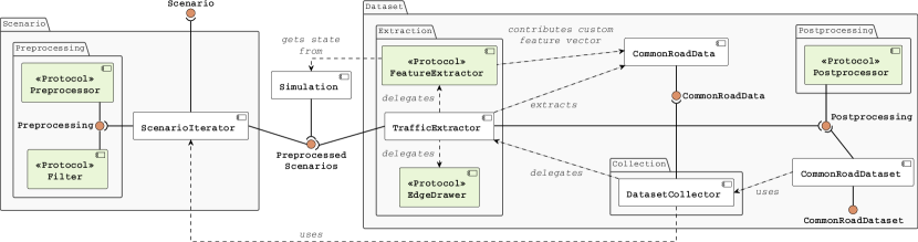
Figure 7: High-level software architecture for cr-geo shown as a UML 2 component diagram [Booch04_uml].

Conforming to the single responsibility principle [Martin17_clean_software], cr-geo is composed of distinct modules with clearly defined roles. To encapsulate volatile processing routines that may require frequent modifications, the strategy pattern [gamma1994design] is employed. This lets the user realize specific behaviors through composition, making it possible to extend the framework to satisfy different requirements and use cases. Users can introduce or substitute implementations without interfering with the rest of the framework, avoiding unintended side effects and minimizing debugging, testing, maintenance, and refactoring efforts.

Next, we introduce the core functionalities of our framework on the basis of these design principles. Tab. III summarizes the options available to customize graph extraction:

Component	Target	Count	Default
Preprocessors	input scenario	many	$\emptyset$
Filters	input scenario	many	$\emptyset$
v2v edge drawer	$\mathcal{E}_{\scalebox{0.85}[0.74]{V}\scalebox{1.12}[1.0]{2}\scalebox{0.85}[0.74]{V}}$	one	VoronoiEdgeDrawer
vtv edge drawer	$\mathcal{E}_{\scalebox{0.85}[0.74]{V}\scalebox{0.85}[0.74]{T}\scalebox{0.85}[0.74]{V}}$	one	CausalEdgeDrawer
Feature extractors	$\mathcal{X}_{\mathcal{V}}$, $\mathcal{X}_{\mathcal{E}}$	many	$\emptyset$
Postprocessors	$\mathcal{G}$	many	$\emptyset$

TABLE III: Summary of cr-geo’s base protocols facilitating user-specified behaviors.

III-B2 Scenario preprocessing and filtering

Our framework supports arbitrary preprocessing and filtering of the input scenarios to ensure that they satisfy the user requirements. As an example, TrafficFilter(min=10) lets users exclude scenarios with less than $10$ vehicles from the collected graph dataset. Further, suppose that we want a higher-fidelity view of the lanelet network, where no lanelet exceeds $20$ meters in length: this can be achieved by using cr-geo’s built-in SegmentLanelets preprocessor, which results in a higher lanelet node density. Using our composition syntax that realizes arbitrary chaining and grouping of preprocessing and filtering operations, these behaviors can be effortlessly combined via
TrafficFilter(min=10) >> SegmentLanelets(size=20).

III-B3 Feature extraction

The extraction of the graph features, i.e., $\mathcal{X}_{\mathcal{V}}$ and $\mathcal{X}_{\mathcal{E}}$, is carried out through feature extractors operating on the scenario objects. The feature extractors receive a simulation object, which provides access to inherent and derived state information of the scenario at the current timestep. By maintaining an internal state, feature extractors also support time-dependent features.

In our framework, we distinguish between node- and edge-level feature extractors, with the latter operating on pairs of entities according to $\mathcal{E}$. In accordance with cr-geo’s guiding design principles, users can devise their own implementation to augment the extracted graphs by arbitrary custom features without modifying the cr-geo source code. To reduce the initial setup time for new users, cr-geo also offers users a selection of pre-configured feature extractor implementations designed to meet the most common needs and requirements.

III-B4 Postprocessors

In contrast to the aforementioned node- and edge-level feature extractors, postprocessors operate directly on the graph instances in a deferred manner. As such, they are intended to supplement the flexibility we concede in the otherwise rigorous graph extraction procedure. User-devised postprocessing procedures can serve numerous practical purposes, e.g.,

• to complement the functionality of feature extractors by facilitating the computation of graph-global features, e.g., an indicator for whether the current traffic scene corresponds to a traffic jam or not;

• to modify the graph structure, e.g., by the removal or insertion of nodes and edges.

The postprocessors are executed after the initial graph extraction, but prior to dataset generation. Furthermore, they can also be applied while loading an existing dataset.

III-B5 Traffic graph extraction

The execution of edge drawing, feature extraction and postprocessing is orchestrated by a traffic extractor, which manages the creation of a CommonRoadData instance at a single timestep $t$. It also handles the declaration of metadata attributes such as node IDs.

The traffic extractor class is complemented by the temporal traffic extractor for the purpose of extracting temporal graph representations. Internally relying on a regular traffic extractor, it maintains a cache of the $n$ preceding ordinary CommonRoadData instances at all times. When called upon, it returns the CommonRoadTemporalData at the current timestep by merging the cached graph sequence into a single entity. The temporal extractor delegates the temporal edge construction to the provided temporal edge drawer and the computation of custom temporal features to the V T V feature extractors provided by the user. The regular and temporal extraction procedures are summarized by Alg. 1 and LABEL:alg:temp-data-creation, respectively.

Algorithm 1 Extraction of CommonRoadData by TrafficExtractor.

Scenario scenario

Edge drawer $D^{\scalebox{0.85}[0.74]{V}\scalebox{1.12}[1.0]{2}\scalebox{0.85}[0.74]{V}}$

Set of feature extractors $\mathcal{F}$

Sequence of postprocessors $\mathcal{P}_{post}$

simulation $\leftarrow$ Simulation$($scenario$)$

Timestep $t$

CommonRoadData

Extract

state $\leftarrow$ simulation$(t)$ $\triangleright$ Current traffic state