Robust Estimation under the Wasserstein Distance

Abstract

We study the problem of robust distribution estimation under the Wasserstein metric, a popular discrepancy measure between probability distributions rooted in optimal transport (OT) theory. We introduce a new outlier-robust Wasserstein distance $\mathsf{W}_{p}^{\varepsilon}$ which allows for $\varepsilon$ outlier mass to be removed from its input distributions, and show that minimum distance estimation under $\mathsf{W}_{p}^{\varepsilon}$ achieves minimax optimal robust estimation risk. Our analysis is rooted in several new results for partial OT, including an approximate triangle inequality, which may be of independent interest. To address computational tractability, we derive a dual formulation for $\mathsf{W}_{p}^{\varepsilon}$ that adds a simple penalty term to the classic Kantorovich dual objective. As such, $\mathsf{W}_{p}^{\varepsilon}$ can be implemented via an elementary modification to standard, duality-based OT solvers. Our results are extended to sliced OT, where distributions are projected onto low-dimensional subspaces, and applications to homogeneity and independence testing are explored. We illustrate the virtues of our framework via applications to generative modeling with contaminated datasets.

1 Introduction

Discrepancy measures between probability distributions are a fundamental constituent of statistical inference, machine learning, and information theory. Among many such measures, Wasserstein distances (Villani, 2003) have recently emerged as a tool of choice for many applications. Specifically, for $p\in[1,\infty)$ and a pair of probability measures $\mu,\nu$ on a metric space $(\mathcal{X},\mathsf{d})$, the $p$-Wasserstein distance between them is

$$\mathsf{W}_{p}(\mu,\nu):=\mathopen{}\mathclose{{}\left(\inf_{\pi\in\Pi(\mu,\nu)}\int_{\mathcal{X}\times\mathcal{X}}\mathsf{d}(x,y)^{p}\,\mathrm{d}\pi(x,y)}\right)^{\frac{1}{p}},$$ (1)

where $\Pi(\mu,\nu)$ is the set of couplings for $\mu$ and $\nu$. The popularity of these metrics stems from a myriad of desirable properties, including rich geometric structure, metrization of the weak topology, robustness to support mismatch, and a convenient dual form. Modern applications of Wasserstein distances include generative modeling (Arjovsky et al., 2017; Gulrajani et al., 2017; Tolstikhin et al., 2018), domain adaptation (Courty et al., 2014, 2016), and robust optimization (Esfahani and Kuhn, 2018; Blanchet et al., 2022; Gao and Kleywegt, 2016).

We consider the problem of robust distribution estimation under the Wasserstein metric. In practice, data can deviate from distributional assumptions due to measurement error, model misspecification, and even malicious outliers. We work under the strong $\varepsilon$-contamination model where, given $n$ independent and identically distributed (i.i.d.) samples from an unknown distribution $\mu$, an adversary arbitrarily modifies an $\varepsilon$-fraction. Given this corrupted data $\tilde{X}_{1},\ldots,\tilde{X}_{n}$, we seek an estimator $\mathsf{T}$ which minimizes the Wasserstein error $\mathsf{W}_{p}\bigl{(}\mathsf{T}(\tilde{X}_{1},\ldots,\tilde{X}_{n}),\mu\bigr{)}$. The motivation to quantify error via $\mathsf{W}_{p}$ stems not only from its fundamental nature as a discrepancy measure between probability distributions, but also from the fact that many properties of $\mu$ vary smoothly under $\mathsf{W}_{p}$ (e.g., if $\mathsf{W}_{p}(\mu,\nu)\leq\delta$, then $\mathopen{}\mathclose{{}\left|\int f\,\mathrm{d}\mu-\int f\,\mathrm{d}\nu}\right|\leq\delta$ for all 1-Lipschitz $f$). We devise a minimax optimal robust estimator by combining minimum distance estimation (MDE)—a classic method for robust statistics—and partial optimal transport (OT), which relaxes the strict marginal constraints of (1) to allow elimination of outliers. Leveraging new contributions to partial OT, we conduct an in-depth theoretical study of the proposed framework, derive minimax optimality guarantees, and develop an accompanying duality theory that enables its practical implementation.

1.1 Contributions

Our estimator is derived via MDE with respect to a robust version of the classical Wasserstein metric. We define the $\varepsilon$-outlier-robust Wasserstein distance by the partial OT problem

$$\mathsf{W}_{p}^{\varepsilon}(\mu,\nu):=\inf_{\begin{subarray}{c}\mu^{\prime},\nu^{\prime}\in\mathcal{M}_{+}(\mathcal{X})\\ \mu^{\prime}\leq\mu,\,\nu^{\prime}\leq\nu\\ \mu^{\prime}(\mathcal{X})=\nu^{\prime}(\mathcal{X})=1-\varepsilon\end{subarray}}\mathsf{W}_{p}\mathopen{}\mathclose{{}\left(\mu^{\prime},\nu^{\prime}}\right),$$ (2)

where $\leq$ denotes setwise inequality and $\mu^{\prime},\nu^{\prime}$ are positive measures that can be heuristically understood as outlier-filtered versions of $\mu,\nu$. In Section 3, we provide a detailed overview of the properties, computation, and structure of $\mathsf{W}_{p}^{\varepsilon}$, including a new approximate triangle inequality for partial OT.

To obtain formal guarantees for robust estimation with $\mathsf{W}_{p}^{\varepsilon}$, we require some prior knowledge about the clean distribution $\mu$ (otherwise, there is no way to distinguish between outliers and inliers). Formally, we assume that $\mu$ belongs to a family $\mathcal{G}$ encoding distributional assumptions, e.g., bounded $q$th moments or sub-Gaussianity. Then, given contaminated samples $\tilde{X}_{1},\dots,\tilde{X}_{n}$ with empirical measure $\tilde{\mu}_{n}\coloneqq\frac{1}{n}\sum_{i=1}^{n}\delta_{\tilde{X}_{i}}$, we propose the minimum distance estimate

$$\mathsf{T}(\tilde{\mu}_{n})\in\operatorname{argmin}_{\nu\in\mathcal{G}}\mathsf{W}_{p}^{\varepsilon}(\nu,\tilde{\mu}_{n}).$$

In Section 4, we show that this procedure achieves minimax optimal risk for a variety of standard families as $n\to\infty$. For the finite-sample case, we show that the attained risk is optimal up to the suboptimality of plug-in estimation under $\mathsf{W}_{p}$, noting that the (sub)optimality of the plug-in estimator is currently an open question in the OT literature. In the related setting where one receives corrupted samples from two distributions, $\mathsf{W}_{p}^{\varepsilon}$ directly serves as a high-quality and efficiently computable estimate for $\mathsf{W}_{p}$ between them, particularly for applications like two-sample/independence testing. Moreover, we show in Section 7 that all of the above results translate to the setting of sliced Wasserstein distances, where distributions are compared along low-dimensional subspaces (Rabin et al., 2011; Lin et al., 2021; Niles-Weed and Rigollet, 2022; Nietert et al., 2022).

In Section 5, we extend the classical Kantorovich dual formulation of $\mathsf{W}_{p}$ to the robust setting. Specifically, we derive a dual representation of $\mathsf{W}_{p}^{\varepsilon}(\mu,\nu)$ that coincides with the Kantorovich dual up to a sup-norm penalty on the optimal potential function. The result holds for arbitrary distributions $\mu,\nu$, without the need for any support/moment assumptions, and suggests an elementary robustification technique for existing dual-based OT solvers by introducing said penalty. In Section 6, we implement $\mathsf{W}_{p}^{\varepsilon}$ via this approach and successfully apply it to generative modeling with contaminated image data.

1.2 Related Work

We review previously proposed notions of robust Wasserstein distances. While some are related to $\mathsf{W}_{p}^{\varepsilon}$, they are not well-suited for large-scale computation via duality nor were they shown to achieve meaningful robust estimation guarantees. In Balaji et al. (2020), similar constraints are imposed with respect to (w.r.t.) general $f$-divergences, but the perturbed measures are restricted to be probability distributions. This results in a more complex dual form (derived by invoking standard Kantorovich duality on the Wasserstein distance between perturbations) and requires optimization over a significantly larger domain. In Mukherjee et al. (2021), robustness w.r.t. the TV distance is added via a regularization term in the objective. This leads to a simple modified primal problem but the corresponding dual requires optimizing over two potentials, even when $p=1$. Additionally, Le et al. (2021) and Nath (2020) consider robustness via Kullback-Leibler (KL) divergence and integral probability metric regularization terms, respectively. The former focuses on Sinkhorn-based primal algorithms and the latter introduces a dual form that is distinct from ours and less compatible with existing duality-based OT computational methods. In Staerman et al. (2021), a median of means approach is used to tackle the dual Kantorovich problem when the contamination fraction $\varepsilon$ vanishes as $n\to\infty$.

The robust OT literature is intimately related to unbalanced OT theory, which addresses transport problems between measures of different mass (Piccoli and Rossi, 2014; Chizat et al., 2018a; Liero et al., 2018; Schmitzer and Wirth, 2019; Hanin, 1992). These formulations are reminiscent of the problem (2) but with regularizers added to the objective (KL being the most studied) rather than incorporated as constraints. Sinkhorn-based primal algorithms (Chizat et al., 2018b) are the standard approach to computation, and these have recently been extended to large-scale machine learning problems via minibatch methods (Fatras et al., 2021). Fukunaga and Kasai (2022) introduces primal-based algorithms for semi-relaxed OT, where marginal constraints for a single measure are replaced with a regularizer in the objective. Partial OT (Caffarelli and McCann, 2010; Figalli, 2010), where only a fraction of mass needs to be moved, is perhaps the most relevant framework. As noted, (2) is itself a partial OT problem, with a $1-\varepsilon$ fraction of mass being transported. However, Caffarelli and McCann (2010) consider a different parameterization of the problem, arriving at a distinct dual, and Figalli (2010) is mostly restricted to quadratic costs with no discussion of duality. Recently, Chapel et al. (2020) explored partial OT for positive-unlabeled learning, but dual-based algorithms were not considered.

There is a long history of learning in the presence of corruptions dating back to the robust statistics community in the 1960s (Huber, 1964). Over the years, many robust and sample-efficient estimators have been designed, particularly for mean and scale parameters (see, e.g., Ronchetti and Huber (2009) for a comprehensive survey). In the theoretical computer science community, much work has focused on achieving optimal rates for robust mean and moment estimation with computationally efficient estimators (Cheng et al., 2019; Diakonikolas and Kane, 2019). Recent statistics work has developed a unified framework for robust estimation based on MDE, which generally achieves sharp population-limit and good finite-sample guarantees for mean and covariance estimation (Zhu et al., 2022). Their analysis centers upon a “generalized resilience” quantity which is also essential to our work (once tailored to the OT setting). Our MDE approach follows their “weaken-the-distance” approach to robust statistics, but with a distinct notion of “weakening” that lends itself better to OT. Finally, Zhu et al. (2022) also consider robust estimation under bounded $\mathsf{W}_{1}$ corruptions, a distinct inference task from that considered here.

2 Preliminaries

Notation.

Let $(\mathcal{X},\mathsf{d})$ be a complete, separable metric space, and denote the diameter of a set $A\subset\mathcal{X}$ by $\operatorname{diam}(A)\coloneqq\sup_{x,y\in A}\mathsf{d}(x,y)$. Write $\operatorname{Lip}_{1}(\mathcal{X})$ for the family of real 1-Lipschitz functions on $\mathcal{X}$. Take $C_{b}(\mathcal{X})$ as the set of continuous, bounded real functions on $\mathcal{X}$, and let $\mathcal{M}(\mathcal{X})$ denote the set of signed Radon measures on $\mathcal{X}$ equipped with the TV norm $\|\mu\|_{\mathsf{TV}}\coloneqq\frac{1}{2}|\mu|(\mathcal{X})$. Let $\mathcal{M}_{+}(\mathcal{X})$ denote the space of finite, positive Radon measures on $\mathcal{X}$. For $\mu,\nu\in\mathcal{M}_{+}(\mathcal{X})$ and $p\in[1,\infty]$, we consider the standard $L^{p}(\mu)$ space with norm $\|f\|_{L^{p}(\mu)}=\mathopen{}\mathclose{{}\left(\int|f|^{p}\,\mathrm{d}\mu}\right)^{1/p}$ and write $\mu\leq\nu$ when $\mu(B)\leq\nu(B)$ for every Borel set $B\subseteq\mathcal{X}$. Denote the shared mass of $\mu$ and $\nu$ by $\mu\land\nu\coloneqq\mu-(\nu-\mu)^{-}$, where $\kappa=\kappa^{+}-\kappa^{-}$ is the Jordan decomposition of $\kappa\in\mathcal{M}(\mathcal{X})$. For $A\subseteq\mathcal{X}$ and $\mu\in\mathcal{M}_{+}(\mathcal{X})$, define $\mu|_{A}=\mu(\cdot\cap A)$.

Let $\mathcal{P}(\mathcal{X})\subset M_{+}(\mathcal{X})$ denote the space of probability measures on $\mathcal{X}$, and take $\mathcal{P}_{p}(\mathcal{X})\coloneqq\{\mu\in\mathcal{P}(\mathcal{X}):\int\mathsf{d}(x,x_{0})^{p}\,\mathrm{d}\mu(x)<\infty\text{ for some $x_{0}\in\mathcal{X}$}\}$ to be those with bounded $p$th moment. Given $\mu,\nu\in\mathcal{P}(\mathcal{X})$, let $\Pi(\mu,\nu)$ denote the set of their couplings, i.e., $\pi\in\mathcal{P}(\mathcal{X}\times\mathcal{X})$ such that $\pi(B\times\mathcal{X})=\mu(B)$ and $\pi(\mathcal{X}\times B)=\nu(B)$, for every Borel set $B$. When $\mathcal{X}=\mathbb{R}^{d}$, we write the covariance matrix for $\mu\in\mathcal{P}_{2}(\mathcal{X})$ as $\Sigma_{\mu}\coloneqq\operatorname{\mathbb{E}}[(X-\operatorname{\mathbb{E}}[X])(X-\operatorname{\mathbb{E}}[X])^{\top}]$ where $X\sim\mu$. We also use $\operatorname{\mathbb{E}}_{\mu}[f(X)]$ to denote the expectation of the random variable $f(X)$ when $X\sim\mu$. We write $a\lor b\coloneqq\max\{a,b\}$, $a\land b\coloneqq\min\{a,b\}$, and use $\lesssim,\gtrsim,\asymp$ to denote inequalities/equality up to absolute constants. We sometimes write $a=O(b)$ and $b=\Omega(a)$ for $a\lesssim b$.

Minimum distance estimation.

Given a distribution family $\mathcal{G}\subseteq\mathcal{P}(\mathcal{X})$ and a statistical distance $\mathsf{D}:\mathcal{P}(\mathcal{X})^{2}\to[0,\infty]$, we define the minimum distance functional $\mathsf{T}_{[\mathcal{G},\mathsf{D}]}:\mathcal{P}(\mathcal{X})\to\mathcal{P}(\mathcal{X})$ by the relation

$$\mathsf{T}_{[\mathcal{G},\mathsf{D}]}(\mu)\in\operatorname{argmin}_{\nu\in\mathcal{G}}\mathsf{D}(\mu,\nu),$$

choosing the representative arbitrarily and assuming no issues with existence. More generally, for any $\delta>0$, we set $\mathsf{T}_{[\mathcal{G},\mathsf{D}]}^{\delta}(\mu)$ to any distribution $\kappa\in\mathcal{G}$ such that $\mathsf{D}(\mu,\kappa)\leq\inf_{\nu\in\mathcal{G}}\mathsf{D}(\mu,\nu)+\delta$. One can view such $\nu$ as a $\delta$-approximate projection of $\mu$ onto the family $\mathcal{G}$ under $\mathsf{D}$. We recall next how MDE can be applied in the contexts of OT and robust statistics.

Optimal transport.

For a lower semi-continuous cost function $c:\mathcal{X}^{2}\to\mathbb{R}$, the optimal transport cost between $\mu,\nu\in\mathcal{M}_{+}(\mathcal{X})$ with $\mu(\mathcal{X})=\nu(\mathcal{X})$ is defined by

$$\mathsf{OT}_{c}(\mu,\nu)\coloneqq\inf_{\pi\in\Pi(\mu,\nu)}\int_{\mathcal{X}^{2}}c\,\mathrm{d}\pi,$$

where $\Pi(\mu,\nu)\coloneqq\{\pi\in\mathcal{M}_{+}(\mathcal{X}^{2}):\pi(\cdot\times\mathcal{X})=\mu,\pi(\mathcal{X}\times\cdot)=\nu\}$. For $p\in[1,\infty)$, the $p$-Wasserstein distance $\mathsf{W}_{p}(\mu,\nu)$ as defined in (1) coincides with $\mathsf{OT}_{c}(\mu,\nu)^{1/p}$ for the cost $c(x,y)\coloneqq\mathsf{d}(x,y)^{p}$.

Some basic properties of $\mathsf{W}_{p}$ are (cf. e.g., (Villani, 2009; Santambrogio, 2015)): (i) the $\inf$ is attained in the definition of $\mathsf{W}_{p}$, i.e., there exists a coupling $\pi^{\star}\in\Pi(\mu,\nu)$ such that $\mathsf{W}_{p}^{p}(\mu,\nu)=\int_{\mathbb{R}^{d}\times\mathbb{R}^{d}}|x-y|^{p}d\pi^{\star}(x,y)$; (ii) $\mathsf{W}_{p}$ is a metric on $\mathcal{P}_{p}(\mathcal{X})$; and (iii) convergence in $\mathsf{W}_{p}$ is equivalent to weak convergence plus convergence of $p$th moments: $\mathsf{W}_{p}(\mu_{n},\mu)\to 0$ if and only if $\mu_{n}\stackrel{{\scriptstyle w}}{{\to}}\mu$ and $\int|x|^{p}d\mu_{n}(x)\to\int|x|^{p}d\mu(x)$.

Wasserstein distances adhere to a dual formulation, which we summarize below. For a function $\varphi:\mathcal{X}\to[-\infty,\infty)$ and symmetric cost function $c:\mathcal{X}^{2}\to\mathbb{R}$, the $c$-transform of $\varphi$ is

$$\varphi^{c}(y)\coloneqq\inf_{x\in\mathcal{X}}\big{[}c(x,y)-\varphi(x)\big{]},\quad y\in\mathbb{R}^{d}.$$

A function $\varphi:\mathcal{X}\to[-\infty,\infty)$, not identically $-\infty$, is called $c$-concave if $\varphi=\psi^{c}$ for some function $\psi:\mathcal{X}\to[-\infty,\infty)$. The following duality holds (Villani, 2009, Theorem 5.9),

$$\mathsf{OT}_{c}(\mu,\nu)=\sup_{\begin{subarray}{c}\varphi,\psi\in C_{b}(\mathcal{X})\\ \varphi(x)+\psi(y)\leq c(x,y)\,\forall x,y\in\mathcal{X}\end{subarray}}\mathopen{}\mathclose{{}\left[\int_{\mathcal{X}}\varphi\,\mathrm{d}\mu+\int_{\mathcal{X}}\psi\,\mathrm{d}\nu}\right]=\sup_{\varphi\in C_{b}(\mathcal{X})}\mathopen{}\mathclose{{}\left[\int_{\mathcal{X}}\varphi\,\mathrm{d}\mu+\int_{\mathcal{X}}\varphi^{c}\,\mathrm{d}\nu}\right],$$ (3)

and there is at least one $c$-concave function $\varphi\in C_{b}(\mathcal{X})$ that attains the supremum in the right-hand side; we call this $\varphi$ an OT potential from $\mu$ to $\nu$ for $\mathsf{OT}_{c}$. A function $\varphi$ is $c$-concave w.r.t. the $\mathsf{W}_{1}$ cost $c(x,y)=\mathsf{d}(x,y)$ if and only if $\varphi\in\mathrm{Lip}_{1}(\mathcal{X})$.

Wasserstein GANs as MDE under $\bm{\mathsf{W}_{1}}$.

A remarkable application of OT to machine learning is generative modeling via the Wasserstein GAN framework, which can be understood as MDE under $\mathsf{W}_{1}$. Given a distribution family $\mathcal{G}$ and the $n$-sample empirical measure $\hat{\mu}_{n}$ of an unknown distribution $\mu$, the $\mathsf{W}_{1}$ minimum distance estimate for $\mu$ given $\hat{\mu}_{n}$ is

$$\mathsf{T}_{[\mathcal{G},\mathsf{W}_{1}]}(\hat{\mu}_{n})=\operatorname{argmin}_{\nu\in\mathcal{G}}\mathsf{W}_{1}(\hat{\mu}_{n},\nu)=\operatorname{argmin}_{\nu\in\mathcal{G}}\sup_{f\in\mathrm{Lip}_{1}(\mathcal{X})}\int_{\mathcal{X}}f\,\mathrm{d}(\hat{\mu}_{n}-\nu).$$

In practice, $\mathcal{G}$ is realized as the push-forward of a standard normal distribution through a parameterized family of neural networks. The resulting estimate is called a generative model, since a minimizing parameter allows one to generate high quality samples from a distribution close to $\mu$, given that $\mathcal{G}$ is a sufficiently rich family. The min-max objective for this problem lends itself well to implementation via alternating gradient-based optimization, and the resulting WGAN framework has supported breakthrough work in generative modeling (Arjovsky et al., 2017; Gulrajani et al., 2017; Tolstikhin et al., 2018). MDE under the Wasserstein metric has also been of general interest in the statistics community due to its generalization guarantees and lack of parametric assumptions (Bassetti et al., 2006; Bernton et al., 2017; Boissard et al., 2015).

Robust statistics and MDE under $\bm{\|\cdot\|_{\mathsf{TV}}}$.

In robust statistics, one seeks to estimate some property of a distribution $\mu$ from contaminated data, generally under the requirement that $\mu\in\mathcal{G}$ for some class $\mathcal{G}\subseteq\mathcal{P}(\mathcal{X})$ encoding distributional assumptions. A common approach for quantifying the error is using a statistical distance $\mathsf{D}:\mathcal{P}(\mathcal{X})^{2}\to[0,\infty]$. In the population-limit version of such tasks, sampling issues are ignored, and we suppose that one observes a contaminated distribution $\tilde{\mu}$ such that $\|\tilde{\mu}-\mu\|_{\mathsf{TV}}\leq\varepsilon$. The information-theoretic complexity of robust estimation in this setting is characterized by the modulus of continuity

$$\mathfrak{m}_{\mathsf{D}}(\mathcal{G},\|\cdot\|_{\mathsf{TV}},\varepsilon)\coloneqq\sup_{\begin{subarray}{c}\mu,\nu\in\mathcal{G}\\ \|\mu-\nu\|_{\mathsf{TV}}\leq\varepsilon\end{subarray}}\mathsf{D}(\mu,\nu),$$

and the associated guarantees are achieved via MDE under the TV norm. This is summarized in the following lemma.

Lemma 1 (Robust estimation via MDE (Donoho and Liu, 1988)).

Fix $\mathcal{G}\subseteq\mathcal{P}(\mathcal{X})$, let $\mu\in\mathcal{G}$, and take any $\tilde{\mu}\in\mathcal{P}(\mathcal{X})$ with $\|\tilde{\mu}-\mu\|_{\mathsf{TV}}\leq\varepsilon$. Then, for any $\nu\in\mathcal{G}$ such that $\|\nu-\tilde{\mu}\|_{\mathsf{TV}}\leq\varepsilon$, including the minimum distance estimate $\mathsf{T}_{[\mathcal{G},\|\cdot\|_{\mathsf{TV}}]}(\tilde{\mu})$, we have

$$\mathsf{D}(\nu,\mu)\leq\mathfrak{m}_{\mathsf{D}}(\mathcal{G},\|\cdot\|_{\mathsf{TV}},2\varepsilon).$$ (4)

The MDE solution satisfies $\|\mathsf{T}_{[\mathcal{G},\|\cdot\|_{\mathsf{TV}}]}(\tilde{\mu})-\tilde{\mu}\|_{\mathsf{TV}}\leq\varepsilon$ because $\|\mu-\tilde{\mu}\|_{\mathsf{TV}}\leq\varepsilon$ and $\mu\in\mathcal{G}$, while inequality (4) holds by the definition of the modulus since $\|\mu-\nu\|_{\mathsf{TV}}\leq\|\mu-\tilde{\mu}\|_{\mathsf{TV}}+\|\tilde{\mu}-\nu\|_{\mathsf{TV}}\leq 2\varepsilon$ and $\mu,\nu\in\mathcal{G}$. In typical cases of interest, it is easy to show that no procedure can obtain estimation error less than $\mathfrak{m}_{\mathsf{D}}(\mathcal{G},\|\cdot\|_{\mathsf{TV}},\varepsilon)$ for all $\mu\in\mathcal{G}$, so this characterization is essentially tight.

Generalized resilience.

Our robustness analysis for OT distances relies on the notion of (generalized) resilience, which was originally proposed for robust mean estimation (Steinhardt et al., 2018; Zhu et al., 2022). Specifically, given a statistical distance $\mathsf{D}:\mathcal{P}(\mathcal{X})^{2}\to[0,\infty]$, we say that $\mu\in\mathcal{P}(\mathcal{X})$ is $(\rho,\varepsilon)$-resilient w.r.t. $\mathsf{D}$ if $\mathsf{D}(\mu,\nu)\leq\rho$ for all distributions $\nu$ with $\nu\leq\frac{1}{1-\varepsilon}\mu$. Resilience is a primary sufficient condition for robust estimation, since it implies immediate bounds on the relevant modulus of continuity.

Lemma 2 (Bounded modulus under resilience (Zhu et al., 2022)).

Let $\mathsf{D}:\mathcal{P}(\mathcal{X})^{2}\to[0,\infty]$ satisfy the triangle inequality, and write $\mathcal{G}$ for the family distributions which are $(\rho,2\varepsilon)$-resilient w.r.t. $\mathsf{D}$. Then we have

$$\mathfrak{m}_{\mathsf{D}}(\mathcal{G},\|\cdot\|_{\mathsf{TV}},\varepsilon)\leq 2\rho.$$

Example 1 (Robust mean estimation).

In robust mean estimation, the error is generally quantified via $\mathsf{D}_{\mathrm{mean}}(\mu,\nu)=\|\operatorname{\mathbb{E}}_{\mu}[X]-\operatorname{\mathbb{E}}_{\nu}[X]\|_{2}$, i.e., we seek an estimate for the mean of an unknown distribution under the $\ell_{2}$ norm. A distribution $\mu$ is $(\rho,\varepsilon)$-resilient w.r.t. $\mathsf{D}_{\mathrm{mean}}$ (or $(\rho,\varepsilon)$-resilient in mean), if $\|\operatorname{\mathbb{E}}_{\mu}[X]-\operatorname{\mathbb{E}}_{\nu}[X]\|_{2}\leq\rho$ for all distributions $\nu\leq\frac{1}{1-\varepsilon}\mu$. For example, if $\mu$ has variance $\sigma$, one can show that $\mu$ is $\bigl{(}O(\sigma\sqrt{\varepsilon}),2\varepsilon\bigr{)}$-resilient in mean; thus its mean can be recovered under TV $\varepsilon$-corruptions up to error $O(\sigma\sqrt{\varepsilon})$. The MDE procedure achieving this risk bound in the population-limit is closely related to efficient finite-sample algorithms based on iterative filtering and spectral reweighting (Diakonikolas et al., 2016; Hopkins et al., 2020).

3 The Robust Wasserstein Distance

Central to our approach for robust estimation is the robust Wasserstein distance $\mathsf{W}_{p}^{\varepsilon}$. After recalling the definition, this section explores $\mathsf{W}_{p}^{\varepsilon}$ for its basic properties in Section 3.1, computation and duality in Section 3.2, and structure of primal and dual optimizers in Section 3.3. Proofs are deferred to Section 8.1. Henceforth, we fix $p\in[1,\infty)$.

Definition 1 (Robust $p$-Wasserstein distance).

The robust $p$-Wasserstein distance with robustness radius $\varepsilon\geq 0$ between distributions $\mu,\nu\in\mathcal{P}(\mathcal{X})$ is defined as

$$\mathsf{W}_{p}^{\varepsilon}(\mu,\nu)\coloneqq\inf_{\begin{subarray}{c}\mu^{\prime},\nu^{\prime}\in\mathcal{M}_{+}(\mathcal{X})\\ \mu^{\prime}\leq\mu,\nu^{\prime}\leq\nu\\ \mu^{\prime}(\mathcal{X})=\nu^{\prime}(\mathcal{X})=1-\varepsilon\end{subarray}}\mathsf{W}_{p}(\mu^{\prime},\nu^{\prime}).$$ (5)

Observe that $\mathsf{W}_{p}^{\varepsilon}$ is a partial OT problem. It filters out an $\varepsilon$-fraction of mass from both measures to avoid over-estimation of the distance due to contamination of either of them.

3.1 Basic Properties

We first identify extreme values of $\mathsf{W}_{p}^{\varepsilon}$ and note its monotonicity in the robustness radius, as summarized in the following proposition.

Proposition 1 (Dependence of $\mathsf{W}_{p}^{\varepsilon}$ on $\varepsilon$).

For any $\mu,\nu\in\mathcal{P}(\mathcal{X})$ and $0<\varepsilon_{1}\leq\varepsilon_{2}<\|\mu-\nu\|_{\mathsf{TV}}$, we have

$$0<\mathsf{W}_{p}^{\varepsilon_{2}}(\mu,\nu)\leq\mathopen{}\mathclose{{}\left(\frac{1-\varepsilon_{2}}{1-\varepsilon_{1}}}\right)^{\!\frac{1}{p}}\mathsf{W}_{p}^{\varepsilon_{1}}(\mu,\nu)\leq\mathsf{W}_{p}^{\varepsilon_{1}}(\mu,\nu)<\infty,$$

with $\mathsf{W}_{p}^{0}(\mu,\nu)=\mathsf{W}_{p}(\mu,\nu)$ and $\mathsf{W}_{p}^{\|\mu-\nu\|_{\mathsf{TV}}}(\mu,\nu)=0$.

Although $\mathsf{W}_{p}^{\varepsilon}$ is defined in terms of mass subtraction, it admits a related mass addition formulation which underlies the main results of this work.

Proposition 2 (Equivalence of mass removal and addition).

For all $\mu,\nu\in\mathcal{P}(\mathcal{X})$, we have

$$\mathsf{W}_{p}^{\varepsilon}(\mu,\nu)=\inf_{\begin{subarray}{c}\mu^{\prime},\nu^{\prime}\in\mathcal{M}_{+}(\mathcal{X})\\ \mu^{\prime}\geq\mu,\,\nu^{\prime}\geq\nu\\ \mu^{\prime}(\mathcal{X})=\nu^{\prime}(\mathcal{X})=1+\varepsilon\end{subarray}}\mathsf{W}_{p}(\mu^{\prime},\nu^{\prime}).$$

The proof relies on the geometric symmetry of the OT distance objective: instead of removing a piece of mass from one measure, we may equivalently add it to the other.

Next, while $\mathsf{W}_{p}^{\varepsilon}$ is not a proper metric, it is non-negative, symmetric, and satisfies an approximate triangle inequality.

Proposition 3 (Approximate triangle inequality).

For $\mu,\nu,\kappa\in\mathcal{P}(\mathcal{X})$ and $0\leq\varepsilon_{1},\varepsilon_{2}\leq 1$,

$$\mathsf{W}_{p}^{\varepsilon_{1}+\varepsilon_{2}}(\mu,\nu)\leq\mathsf{W}_{p}^{\varepsilon_{1}}(\mu,\kappa)+\mathsf{W}_{p}^{\varepsilon_{2}}(\kappa,\nu).$$ (6)

The proof is non-trivial but can be explained concisely with a set of diagrams.

Figure 1: Diagrams illustrating the $\mathsf{W}_{p}$ triangle inequality (left) and Proposition 2 (right).

Proof sketch.

In what follows, each diagram is a collection of nodes and labeled edges corresponding to a statement about a set of non-negative measures. Blue arrows between diagrams indicate implications between their respective statements. We start by describing this visual formalism.

Nodes and edges: Each node is an element of $\mathcal{M}_{+}(\mathcal{X})$, and each edge describes a relationship between measures.

Vertical positioning: The vertical positioning within a diagram indicates relative total mass, i.e., if a node $\mu$ is above a node $\nu$, then $\mu(\mathcal{X})>\nu(\mathcal{X})$.

Solid edges: A solid horizontal line between $\mu,\nu\in\mathcal{M}_{+}(\mathcal{X})$ with label $W$ indicates that $\mu(\mathcal{X})=\nu(\mathcal{X})$ and $\mathsf{W}_{p}(\mu,\nu)\leq W$ (the horizontal ordering is inconsequential).

Squiggly edges: A squiggly line between $\mu,\nu\in\mathcal{M}_{+}(\mathcal{X})$ with label $\varepsilon$ indicates that $\|\mu-\nu\|_{\mathsf{TV}}\leq 2\varepsilon$ (note the factor of two).

Dashed edges: A dashed line between $\mu,\nu\in\mathcal{M}_{+}(\mathcal{X})$ with $\mu$ above $\nu$ and label $\varepsilon$ indicates that $\|\mu-\nu\|_{\mathsf{TV}}\leq 2\varepsilon$ and further $\nu\leq\mu$ (i.e., $\mu$ is obtained by adding $\varepsilon$ mass to $\nu$).

Unlabeled nodes: Unlabeled nodes corresponds to existential quantifiers over measures, i.e., a diagram with unlabeled nodes represents the statement that the diagram is true for some assignment of non-negative measures to the unlabeled nodes.

As a warm-up, we depict the triangle inequality for $\mathsf{W}_{p}$ and Proposition 2 in Fig. 1. More precisely, the right pair of diagrams encodes the following statement: “Let $\mu,\nu\in\mathcal{M}_{+}(\mathcal{X})$ such that $\mu(\mathcal{X})=\nu(\mathcal{X})$. Then there exist $\alpha,\beta\in\mathcal{M}_{+}(\mathcal{X})$ such that $\alpha\leq\mu$, $\beta\leq\nu$, $\alpha(\mathcal{X})=\beta(\mathcal{X})\geq\mu(\mathcal{X})-\varepsilon$, and $\mathsf{W}_{p}(\alpha,\beta)\leq W$ if and only if there exist $\alpha^{\prime},\beta^{\prime}\in\mathcal{M}_{+}(\mathcal{X})$ such that $\alpha^{\prime}\geq\mu$, $\beta^{\prime}\geq\nu$, $\alpha^{\prime}(\mathcal{X})=\beta^{\prime}(\mathcal{X})\leq\mu(\mathcal{X})+\varepsilon$, and $\mathsf{W}_{p}(\alpha^{\prime},\beta^{\prime})\leq W$.”

With this same notation, the proof of Proposition 3 is summarized in Fig. 2. To start, suppose without loss of generality that $\varepsilon_{1}\leq\varepsilon_{2}$, and write $W_{1}\coloneqq\mathsf{W}_{p}^{\varepsilon_{1}}(\mu,\kappa)$ and $W_{2}\coloneqq\mathsf{W}_{p}^{\varepsilon_{2}}(\kappa,\nu)$. Then the statement captured by the top-left diagram holds. Implication (1) holds because removing $\varepsilon_{2}$ mass from $\kappa$ can be split into two steps: first removing $\varepsilon_{2}-\varepsilon_{1}$ mass and then removing $\varepsilon_{1}$ more mass. Implication (2) corresponds to the right pair of warm-up diagrams. Implication (3) follows by Lemma 4, presented and proven in Section 8.1, and corresponds to swapping two pairs of edges. Implication (4) holds by the $\mathsf{W}_{p}$ and TV triangle inequalities. Finally, implication (5) holds by Lemma 5 in Section 8.1, which is a simple consequence of Proposition 2. The bottom-right figure implies that $\mathsf{W}_{p}^{\varepsilon_{1}+\varepsilon_{2}}(\mu,\nu)\leq W_{1}+W_{2}=\mathsf{W}_{p}^{\varepsilon_{1}}(\mu,\kappa)+\mathsf{W}_{p}^{\varepsilon_{2}}(\kappa,\nu)$. ∎

Figure 2: A visual proof of Proposition 3.

3.2 Computation and Duality

For computation, we recall a useful reduction from partial OT to standard OT with an augmented space and cost function (Chapel et al., 2020). This result enables employing computational methods designed for standard OT towards the partial OT problem.

Proposition 4 ($\mathsf{W}_{p}^{\varepsilon}$ via standard OT with augmented spaces, Chapel et al. (2020)).

Let $\bar{\mathcal{X}}$ denote the disjoint union $\mathcal{X}\sqcup\{\bar{x}\}$ of $\mathcal{X}$ with a dummy point $\bar{x}$, and define the augmented cost function $c:\bar{\mathcal{X}}^{2}\to[0,\infty]$ by

$$\bar{c}(x,y)=\begin{cases}\mathsf{d}(x,y)^{p},&x,y\in\mathcal{X}\\ 0,&x\in\mathcal{X},y=\bar{x}\ \mbox{or}\ y\in\mathcal{X},x=\bar{x}\\ \infty.&x=y=\bar{x}\end{cases}$$

For any $\mu,\nu\in\mathcal{P}(\mathcal{X})$, we have $\mathsf{W}_{p}^{\varepsilon}(\mu,\nu)=\mathsf{OT}_{\bar{c}}(\mu+\varepsilon\delta_{\bar{x}},\nu+\varepsilon\delta_{\bar{x}})$.

One may thus compute $\mathsf{W}_{p}^{\varepsilon}$ between empirical measures by applying methods for standard OT to this augmented space, e.g., linear programming for an exact solution or Sinkhorn methods for an approximate solution (see Peyré and Cuturi (2019) for a thorough discussion of computational OT). In this case, $\bar{c}(\bar{x},\bar{x})$ can be taken to be a sufficiently large but finite constant. The only shortfall to this approach is that the augmented cost is no longer induced by a Euclidean norm, which is important for some dual-based OT applications like WGAN. Fortunately, we show in the following theorem that $\mathsf{W}_{p}^{\varepsilon}$ also admits a modified Kantorivich-type dual.

[Dual form]theoremRWpdual For $0<\varepsilon\leq 1$ and $\mu,\nu\in\mathcal{P}(\mathcal{X})$, we have

$$\mathsf{W}_{p}^{\varepsilon}(\mu,\nu)^{p} =\sup_{\begin{subarray}{c}\varphi\in C_{b}(\mathcal{X})\end{subarray}}\int_{\mathcal{X}}\varphi\,\mathrm{d}\mu+\int_{\mathcal{X}}\varphi^{c}\,\mathrm{d}\nu-2\varepsilon\|\varphi\|_{\infty}$$ (7)

$$=\sup_{\begin{subarray}{c}\varphi\in C_{b}(\mathcal{X})\end{subarray}}\int_{\mathcal{X}}\varphi\,\mathrm{d}\mu+\int_{\mathcal{X}}\varphi^{c}\,\mathrm{d}\nu-\varepsilon\mathopen{}\mathclose{{}\left(\sup_{x\in\mathcal{X}}\varphi(x)-\inf_{x\in\mathcal{X}}\varphi(x)}\right),$$

and the suprema are achieved by $\varphi\in C_{b}(\mathcal{X})$ with $\varphi=(\varphi^{c})^{c}$.

This new formulation differs from the classic dual (3) by a sup-norm penalty for the potential function and its lack of moment requirements on $\mu$ and $\nu$. Recall that when $p=1$, $\varphi=(\varphi^{c})^{c}$ exactly when $\varphi$ is 1-Lipschitz, with $\varphi^{c}=-\varphi$. We provide proof details and discussion of this result in Section 5.

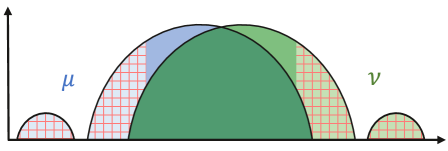
Figure 3: Visualization of Proposition 5: The gridded light blue and green regions each have mass $\varepsilon$, respectively, and are removed to obtain optimal $\mu^{\prime}$ and $\nu^{\prime}$ for $\mathsf{W}_{1}^{\varepsilon}$. No mass need be removed from the dark region designating $\mu\land\nu$.

3.3 Structure of Optimizers

Given the primal and dual formulations, it is natural to ask how optimal solutions to these problems are related. We first observe that optimizers for the primal form (5) exist (dual solutions exist by Proposition 4) and then uncover their interplay with optimal dual potentials.

Proposition 5 (Existence of minimizers).

For any $\mu,\nu\in\mathcal{P}(\mathcal{X})$, the infimum in (5) is achieved, and there are minimizers $\mu^{\prime}\leq\mu$ and $\nu^{\prime}\leq\nu$ such that $\mu^{\prime},\nu^{\prime}\geq\mu\land\nu$.

To show that the infimum is attained, we prove that the constraint set is compact and that the objective is lower-semicontinuous w.r.t. the weak topology of measures. The existence of minimizers bounded from below by $\mu\land\nu$ is illustrated in Fig. 3. This is easy to prove when $p=1$, since $\mathsf{W}_{1}(\mu,\nu)$ is a function of $\mu-\nu$, and was shown in Figalli (2010) for $p=2$ when $\mu$ and $\nu$ are absolutely continuous w.r.t. the Lebesgue measure. However, the general result is not straightforward and our proof requires a discretization argument.

Proposition 6 (Interpreting maximizers).

Fix $\mu,\nu\in\mathcal{P}(\mathcal{X})$. If $f\in C_{b}(\mathcal{X})$ maximizes (7) and $\mu^{\prime},\nu^{\prime}\in\mathcal{M}_{+}(\mathcal{X})$ minimize (5), then $\operatorname{spt}(\mu-\mu^{\prime})\subseteq\operatorname{argmax}(f)$ and $\operatorname{spt}(\nu-\nu^{\prime})\subseteq\operatorname{argmin}(f)$.

capposition=beside,capbesideposition=top,right,capposition=bottom

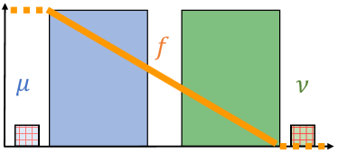
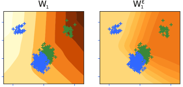
Figure 4: Optimal potentials: (left) 1D densities plotted with their optimal potential for the $\mathsf{W}_{1}^{\varepsilon}$ dual problem; (right) contour plots for optimal dual potentials to $\mathsf{W}_{1}$ and $\mathsf{W}_{1}^{\varepsilon}$ between 2D Gaussian mixtures. Observe how optimal potentials for the robust dual are flat over outlier mass.

Thus, the extremal level sets of any maximizing dual potential encode the location of mass removed in the primal problem, as depicted in Fig. 4. In fact, optimal perturbations $\mu-\mu^{\prime}$ and $\nu-\nu^{\prime}$ are sometimes determined exactly by an optimal potential $f$, often taking the form $\mu|_{\operatorname{argmax}(f)}$ and $\nu|_{\operatorname{argmax}(f)}$ (though not always; we discuss this in Section 8.1).

4 Robust Estimation under $\bm{\mathsf{W}_{p}}$

We now specify the problem of robust distribution estimation under $\mathsf{W}_{p}$, which is at the core of this work. Let $X_{1},\dots,X_{n}$ be i.i.d. samples from an unknown distribution $\mu\in\mathcal{P}(\mathcal{X})$, with corresponding empirical measure $\hat{\mu}_{n}=\frac{1}{n}\sum_{i=1}^{n}\delta_{X_{i}}$. Under the strong $\varepsilon$-contamination model, an adversary observes these samples and produces corrupted samples $\tilde{X}_{1},\dots,\tilde{X}_{n}$ with empirical measure $\tilde{\mu}_{n}$, such that the contamination fraction $\|\tilde{\mu}_{n}-\hat{\mu}_{n}\|_{\mathsf{TV}}=\frac{1}{n}\sum_{i=1}^{n}\mathds{1}{\bigl{\{}\tilde{X}_{i}\neq X_{i}\bigr{\}}}$ is at most $\varepsilon$. We seek an estimate $\mathsf{T}(\tilde{\mu}_{n})\in\mathcal{P}(\mathcal{X})$ for $\mu$ that minimizes the error $\mathsf{W}_{p}\bigl{(}\mathsf{T}(\tilde{\mu}_{n}),\mu\bigr{)}$. The problem formulation is as follows.

Error and risk.

The adversarial corruption process is a measurable transformation of the clean samples and some independent (but otherwise arbitrary) source of randomness. Write $\mathcal{M}^{\mathrm{adv}}_{n}(\mu,\varepsilon)$ for the family of all joint distributions $\mathbb{P}_{n}\in\mathcal{P}(\mathcal{X}^{n})$ of corrupted data $\{\tilde{X}_{i}\}_{i=1}^{n}$ that can be obtained by this procedure. Note that the modified samples, of which there are at most $\varepsilon n$, may be highly correlated. Fixing any estimator $\mathsf{T}$ depending only on the corrupted data (and possibly independent randomness), we define its $n$-sample robust estimation error by

$$R_{p,n}(\mathsf{T},\mu,\varepsilon)\coloneqq\inf\left\{\tau\geq 0:\sup_{\mathbb{P}_{n}\in\mathcal{M}_{n}^{\mathrm{adv}}(\mu,\varepsilon)}\mathbb{P}_{n}\Bigl{(}\mathsf{W}_{p}\bigl{(}\mathsf{T}(\tilde{\mu}_{n}),\mu\bigr{)}>\tau\Bigr{)}<\frac{1}{10}\right\}.$$

By definition, the error incurred by $\mathsf{T}$ under $\varepsilon$-contamination is bounded by $R_{p,n}(\mathsf{T},\mu,\varepsilon)$ with probability at least $9/10$. No estimator can obtain finite error for all distributions, so we often require that $\mu$ belongs to a family $\mathcal{G}\subseteq\mathcal{P}(\mathcal{X})$ encoding distributional assumptions. For this setting, we define the finite-sample robust estimation risk $R_{p,n}(\mathsf{T},\mathcal{G},\varepsilon)\coloneqq\smash{\sup_{\mu\in\mathcal{G}}R_{p,n}(\mathsf{T},\mu,\varepsilon)}$ and set $R_{p,n}(\mathcal{G},\varepsilon)\coloneqq\inf_{\mathsf{T}}R_{p,n}(\mathsf{T},\mathcal{G},\varepsilon)$ as the finite-sample minimax risk.

The estimator.

To solve the estimation task, we perform MDE using $\mathsf{W}_{p}^{\varepsilon}$, projecting $\tilde{\mu}_{n}$ onto the clean family $\mathcal{G}$ under the robust distance. That is, we consider the estimate

$$\mathsf{T}_{[\mathcal{G},\mathsf{W}_{p}^{\varepsilon}]}(\tilde{\mu}_{n})\in\operatorname{argmin}_{\nu\in\mathcal{G}}\mathsf{W}_{p}^{\varepsilon}(\tilde{\mu}_{n},\nu).$$

To study the performance of MDE, we begin by analyzing a population-limit version of the problem where measures are observed directly rather than via sampling. In Section 4.1, we introduce a resilience-type condition which characterizes population-limit minimax risk for a variety of standard distribution classes, and we show that this risk is attained by MDE under $\mathsf{W}_{p}^{\varepsilon}$. In Section 4.2, we return to the finite-sample regime and prove that MDE under $\mathsf{W}_{p}^{\varepsilon}$ still achieves near-optimal risk bounds. Finally, in Section 4.3, we consider $\mathsf{W}_{p}^{\varepsilon}$ as a stand-alone estimator for $\mathsf{W}_{p}$, where it achieves optimal guarantees is some regimes. Proofs for this section are deferred to Section 8.2.

Remark 1 (Alternative robust distances).

We can analogously define an asymmetric distance $\mathsf{W}_{p}^{\varepsilon_{\mu},\varepsilon_{\nu}}$ with distinct robustness radii, so that $\mathsf{W}_{p}^{\varepsilon}=\mathsf{W}_{p}^{\varepsilon,\varepsilon}$. Extensions of our main results to this setting are presented in Section A.1. In particular, the risk bounds in this section all hold for MDE under the one-sided robust distance $\mathsf{W}_{p}^{\varepsilon}(\mu\|\nu)\coloneqq\mathsf{W}_{p}^{\varepsilon,0}(\mu,\nu)$. We apply this version for generative modeling experiments (see Section 6), but presently stick to $\mathsf{W}_{p}^{\varepsilon}$ since its symmetry leads to cleaner analysis. Another alternative is $\mathsf{W}_{p}^{\varepsilon,\mathsf{TV}}(\mu,\nu)\coloneqq\inf_{\mu^{\prime},\nu^{\prime}\in\mathcal{P}(\mathcal{X}):\|\mu^{\prime}-\mu\|_{\mathsf{TV}},\|\nu^{\prime}-\nu\|_{\mathsf{TV}}\leq\varepsilon}\mathsf{W}_{p}(\mu^{\prime},\nu^{\prime})$, which was previously examined by Balaji et al. (2020). Our risk bounds all hold for MDE under this alternative distance as well. However, the duality formulation given in Proposition 4 does not extend to $\mathsf{W}_{p}^{\varepsilon,\mathsf{TV}}$. This renders $\mathsf{W}_{p}^{\varepsilon}$ favorable from a computational perspective and motivates our focus on it as the figure of merit.

4.1 Population-Limit Guarantees and Resilience

Before analyzing finite-sample risk, we characterize a baseline risk that is unavoidable even with unlimited samples. Formally, given $\mu$ belonging to a clean family $\mathcal{G}\subseteq\mathcal{P}(\mathcal{X})$, we consider the task of estimating $\mu$ under $\mathsf{W}_{p}$ from a contaminated distribution $\tilde{\mu}$ with $\|\tilde{\mu}-\mu\|_{\mathsf{TV}}\leq\varepsilon$. Given a map $\mathsf{T}:\mathcal{P}(\mathcal{X})\to\mathcal{P}(\mathcal{X})$, we define its population-limit robust estimation error as

$$R_{p,\infty}(\mathsf{T},\mu,\varepsilon)\coloneqq\sup_{\begin{subarray}{c}\mu\in\mathcal{G},\,\tilde{\mu}\in\mathcal{P}(\mathcal{X})\\ \|\tilde{\mu}-\mu\|_{\mathsf{TV}}\leq\varepsilon\end{subarray}}\mathsf{W}_{p}\bigl{(}\mathsf{T}(\tilde{\mu}),\mu\bigr{)}.$$

As before, we define minimax risk as $R_{p,\infty}(\mathcal{G},\varepsilon)=\inf_{\mathsf{T}}\sup_{\mu\in\mathcal{G}}R_{p,\infty}(\mathsf{T},\mu,\varepsilon)$, and MDE corresponds to the estimator $\mathsf{T}=\mathsf{T}_{[\mathcal{G},\mathsf{W}_{p}^{\varepsilon}]}$. In this regime, however, the procedure simplifies considerably; as $\inf_{\nu\in\mathcal{G}}\mathsf{W}_{p}^{\varepsilon}(\tilde{\mu},\nu)\leq\mathsf{W}_{p}^{\varepsilon}(\tilde{\mu},\mu)=0$, the minimum distance estimate satisfies $\mathsf{W}_{p}^{\varepsilon}(\mathsf{T}(\tilde{\mu}),\tilde{\mu})=0$, or equivalently $\|\mathsf{T}(\tilde{\mu})-\tilde{\mu}\|_{\mathsf{TV}}\leq\varepsilon$. Thus, by Lemma 2, this estimator matches the performance of MDE under the TV norm, i.e., $\mathsf{T}=\mathsf{T}_{[\mathcal{G},{\|\cdot\|_{\mathsf{TV}}}]}$, and we have recovered the standard approach to population-limit robust statistics outlined in Section 2.

Without restrictions on $\mathcal{G}$, the risk $R_{p,\infty}(\mathcal{G},\varepsilon)$ may be unbounded, so we now introduce a natural distributional assumption under which accurate estimation is possible, instantiating generalized resilience for the present setting.

Definition 2 (Resilience w.r.t. $\mathsf{W}_{p}$).

Let $0\leq\varepsilon<1$ and $\rho\geq 0$. A distribution $\mu\in\mathcal{P}(\mathcal{X})$ is called $(\rho,\varepsilon)$-resilient w.r.t. $\mathsf{W}_{p}$ if $\mathsf{W}_{p}(\mu,\mu^{\prime})\leq\rho$ for all $\mu^{\prime}\in\mathcal{P}(\mathcal{X})$ such that $\mu^{\prime}\leq\frac{1}{1-\varepsilon}\mu$. Write $\mathcal{W}_{p}(\rho,\varepsilon)$ for the family of all such distributions.

That is, $\mu$ belongs to $\mathcal{W}_{p}(\rho,\varepsilon)$ if deleting an $\varepsilon$-fraction of mass from $\mu$ and renormalizing (equivalently, conditioning on an event with probability $1-\varepsilon$) leads to change at most $\rho$ in $\mathsf{W}_{p}$. In particular, this implies that $\mu$ has finite $p$th moments; otherwise, such change could be infinite. Lemma 2 then gives the following.

Proposition 7 (Bounded risk under resilience).

Let $0\leq\varepsilon<1/2$ and $\mathcal{G}\subseteq\mathcal{W}_{p}(\rho,2\varepsilon)$. Then $R_{p,\infty}(\mathcal{G},\varepsilon)\leq 2\rho$, and this risk is achieved by the estimators $\mathsf{T}_{[\mathcal{G},\mathsf{W}_{p}^{\varepsilon}]}$ and $\mathsf{T}_{[\mathcal{G},\|\cdot\|_{\mathsf{TV}}]}$.

While resilience w.r.t. $\mathsf{W}_{p}$ is a high-level condition, we can precisely quantify it for many families of interest. Moreover, the resulting upper risk bounds from Proposition 7 are often tight. In particular, for $\sigma\geq 0$ and $q\geq 1$, we consider the class $\mathcal{G}_{q}(\sigma)$ of distributions $\mu\in\mathcal{P}(\mathcal{X})$ such that $\operatorname{\mathbb{E}}_{\mu}[\mathsf{d}(X,x_{0})^{q}]\leq\sigma^{q}$ for some $x_{0}\in\mathcal{X}$, i.e., those with centered absolute $q$th moments bounded by $\sigma$. When $\mathcal{X}=\mathbb{R}^{d}$, we further consider the following standard families of sub-Gaussian distributions and those with a bounded covariance matrix, namely:

$$\begin{split}\mathcal{G}_{\mathrm{subG}}(\sigma)&\coloneqq\mathopen{}\mathclose{{}\left\{\mu\in\mathcal{P}(\mathbb{R}^{d}):\operatorname{\mathbb{E}}_{\mu}\mathopen{}\mathclose{{}\left[\exp(|\langle\theta,X-\operatorname{\mathbb{E}}_{\mu}[X]\rangle|^{2}/\sigma^{2})}\right]\leq 2\>\>\forall\theta\in\mathbb{S}^{d-1}}\right\},\\ \mathcal{G}_{\mathrm{cov}}(\sigma)&\coloneqq\mathopen{}\mathclose{{}\left\{\mu\in\mathcal{P}(\mathbb{R}^{d}):\Sigma_{\mu}\preceq\sigma^{2}\mathrm{I}_{d}}\right\}.\end{split}$$ (8)

We now state tight population-limit minimax risk bounds for these concrete classes.

Theorem 1 (Population-limit minimax risk).

For $0\leq\varepsilon\leq 0.49$, we have

$$R_{p,\infty}(\mathcal{G},\varepsilon)\asymp\begin{cases}\sigma\varepsilon^{\frac{1}{p}-\frac{1}{q}},&\!\!\text{if $\mathcal{G}=\mathcal{G}_{q}(\sigma)$ for $q\!>\!p$ and $\,\exists\,x,y\in\mathcal{X}\!:\!\mathsf{d}(x,y)=\sigma\varepsilon^{-\frac{1}{q}}$}\\ \sigma\sqrt{d+p+\log\mathopen{}\mathclose{{}\left(\frac{1}{\varepsilon}}\right)}\,\varepsilon^{\frac{1}{p}},&\text{\!\!if $\mathcal{X}=\mathbb{R}^{d}$ and $\mathcal{G}=\mathcal{G}_{\mathrm{subG}}(\sigma)$}\\ \sigma\sqrt{d}\,\varepsilon^{\frac{1}{p}-\frac{1}{2}},&\text{\!\!if $\mathcal{X}=\mathbb{R}^{d}$, $p<2$, and $\mathcal{G}=\mathcal{G}_{\mathrm{cov}}(\sigma)$}\\ \end{cases}$$

and these risks are achieved by the estimators $\mathsf{T}_{[\mathcal{G},\mathsf{W}_{p}^{\varepsilon}]}$ and $\mathsf{T}_{[\mathcal{G},\|\cdot\|_{\mathsf{TV}}]}$.

For the upper bounds, we show in Section 8.2.1 that resilience w.r.t. $\mathsf{W}_{p}$ is implied by standard mean resilience of the $p$th power of the metric $\mathsf{d}$ and then apply Proposition 7. This yields the risk bound for $\mathcal{G}_{q}(\sigma)$, and we then observe that $\mathcal{G}_{\mathrm{subG}}(\sigma)\subseteq\mathcal{G}_{p\lor\log(1/\varepsilon)}\bigl{(}\sqrt{d+p\lor\log(1/\varepsilon)}\bigr{)}$ and $\mathcal{G}_{\mathrm{cov}}(\sigma)\subseteq\mathcal{G}_{2}\bigl{(}\sqrt{d}\sigma\bigr{)}$. For the lower bounds, we use that $R_{p,\infty}(\mathcal{G},\varepsilon)\geq\frac{1}{2}\mathsf{W}_{p}(\mu,\nu)$ for any $\mu,\nu\in\mathcal{G}$ with $\|\mu-\nu\|_{\mathsf{TV}}\leq\varepsilon$, i.e., it is impossible to distinguish between such distributions. When $\mathcal{G}=\mathcal{G}_{q}(\sigma)$, for example, consider $\mu=\delta_{x},\nu=(1-\varepsilon)\delta_{x}+\varepsilon\delta_{y}$ for some $x,y\in\mathcal{X}$. Then we have $\operatorname{\mathbb{E}}_{\mu}[\mathsf{d}(X,x)^{q}]=0$, $\operatorname{\mathbb{E}}_{\nu}[\mathsf{d}(X,x)^{q}]=\varepsilon\mathsf{d}(x,y)^{q}$, and $\mathsf{W}_{p}(\mu,\nu)=\varepsilon^{1/p}\mathsf{d}(x,y)$. By selecting $d(x,y)=\sigma\varepsilon^{-1/q}$, the maximal distance for which $\mu,\nu\in\mathcal{G}_{q}(\sigma)$, we obtain the tight lower bound of $R_{p,\infty}(\mathcal{G}_{q}(\sigma),\varepsilon)\gtrsim\mathsf{W}_{p}(\mu,\nu)=\sigma\varepsilon^{1/p-1/q}$. Lower bounds for classes $\mathcal{G}_{\mathrm{subG}}(\sigma)$ and $\mathcal{G}_{\mathrm{cov}}(\sigma)$ follow by considering appropriate Gaussian mixtures.

Remark 2 (Comparison to mean resilience).

When $\mathcal{X}=\mathbb{R}^{d}$, the corresponding rates for mean resilience and population-limit minimax risk for robust mean estimation are $O\big{(}\varepsilon\sqrt{\log(1/\varepsilon)}\big{)}$ and $O(\sqrt{\varepsilon})$ for the sub-Gaussian and bounded covariance settings, respectively (see, e.g., Steinhardt et al. (2018)). These match our bounds for $\mathsf{W}_{1}$ up to a dependence on $\sqrt{d}$, which we interpret as a reflection of the high-dimensional structure of the Wasserstein distance.

4.2 Finite-Sample Guarantees

We now return to the original finite-sample setting. The following result provides an unconditional lower bound and a resilience-based upper bound for minimax risk via MDE.

Theorem 2 (Finite-sample minimax risk).

For $0\leq\varepsilon\leq 0.49$ and $\mathcal{G}\subseteq\mathcal{P}(\mathcal{X})$, we have

$$R_{p,n}(\mathcal{G},\varepsilon)\gtrsim R_{p,\infty}(\mathcal{G},\varepsilon/5)+R_{p,n}(\mathcal{G},0).$$

For $\mu\in\mathcal{G}\subseteq\mathcal{W}_{p}(\rho,2\varepsilon)$, the risk of the minimum distance estimator $\mathsf{T}_{[\mathcal{G},\mathsf{W}_{p}^{\varepsilon}]}^{\delta}$ is bounded as

$$R_{p,n}(\mathsf{T}_{[\mathcal{G},\mathsf{W}_{p}^{\varepsilon}]}^{\delta},\mu,\varepsilon)\lesssim\rho+\delta+\operatorname{\mathbb{E}}[\mathsf{W}_{p}(\hat{\mu}_{n},\mu)].$$

Consequently, taking $\delta=0$, we have $R_{p,n}(\mathcal{G},\varepsilon)\lesssim\rho+\sup_{\mu\in\mathcal{G}}\operatorname{\mathbb{E}}[\mathsf{W}_{p}(\hat{\mu}_{n},\mu)]$.

The lower bound formalizes the intuitive notion that finite-sample robust estimation is harder than both population-limit robust estimation and finite-sample standard estimation. The upper bound shows that the risk bound of Proposition 7 translates to the finite-sample setting up to empirical convergence error. For the distribution families considered in Theorem 1, these risk bounds match up to the gap between $R_{p,n}(\mathcal{G},0)$ and $\sup_{\mu\in\mathcal{G}}\operatorname{\mathbb{E}}[\mathsf{W}_{p}(\hat{\mu}_{n},\mu)]$, i.e., up to the sub-optimality of plug-in estimation under $\mathsf{W}_{p}$. To the best of our knowledge, it is unknown whether this gap can be closed. Under the further assumption of smooth densities, the plug-in estimator is known to be suboptimal and the gap from optimality has been characterized (Niles-Weed and Berthet, 2022); optimization for this regime is beyond the scope of this work.

Corollary 1 (Concrete finite-sample risk bounds).

Let $0\leq\varepsilon\leq 0.49$, $q>p$, $\mathcal{X}=\mathbb{R}^{d}$ for $d>2p$, and $\mathcal{G}\in\{\mathcal{G}_{q}(\sigma),\mathcal{G}_{\mathrm{subG}}(\sigma),\mathcal{G}_{\mathrm{cov}}(\sigma)\}$. If $\mathcal{G}=\mathcal{G}_{q}(\sigma)$, further suppose that $d>(1/p-1/q)^{-1}$, while if $\mathcal{G}=\mathcal{G}_{\mathrm{cov}}(\sigma)$, assume that $p<2$ and $d>(1/p-1/2)^{-1}$. Then there exist constants $C_{1},C_{2}>0$ depending only on $p$, $q$, and $d$ such that

$$R_{p,\infty}(\mathcal{G},\varepsilon)+C_{1}\sigma n^{-\frac{1}{d}}\lesssim R_{p,n}(\mathcal{G},\varepsilon)\lesssim R_{p,\infty}(\mathcal{G},\varepsilon)+C_{2}\sigma n^{-\frac{1}{d}},$$

and the upper risk bound is achieved by the minimum distance estimator $\mathsf{T}_{[\mathcal{G},\mathsf{W}_{p}^{\varepsilon}]}$.

We view the upper bound of Theorem 2 as a primary contribution of this work. It has two merits which are essential for meaningful guarantees in practice. First, we only need to perform approximate MDE, as a slack of $\delta$ in optimization only worsens our final bound by $O(\delta)$. Second, the empirical approximation term depends only on the clean measure $\mu$ and can be controlled even under heavy-tailed contamination. If $\mu$ further has upper $p$-Wasserstein dimension $d_{\star}$ in the sense of Weed and Bach (2019) then the $n^{-1/d}$ rate of Corollary 1 can be improved to $n^{-1/d_{\star}}$. We sketch the proof below, deferring full details to Section 8.2.2.

Proof sketch of Theorem 2.

Our proof follows the “weaken the distance” approach to robust statistics formalized in Zhu et al. (2022). We observe that analysis of MDE under the TV distance, as applied to obtain population-limit upper risk bounds, fails in the finite-sample setting because $\|\hat{\mu}_{n}-\mu\|_{\mathsf{TV}}$ may be large. In particular, $\tilde{\mu}_{n}$ cannot be viewed as a small TV perturbation of $\mu$, even though $\|\tilde{\mu}_{n}-\hat{\mu}_{n}\|_{\mathsf{TV}}\leq\varepsilon$. On the other hand, by Proposition 3, we can bound $\mathsf{W}_{p}^{\varepsilon}(\tilde{\mu}_{n},\mu)\leq\mathsf{W}_{p}^{\varepsilon}(\tilde{\mu}_{n},\hat{\mu}_{n})+\mathsf{W}_{p}(\hat{\mu}_{n},\mu)=\mathsf{W}_{p}(\hat{\mu}_{n},\mu)$, which is small with high probability; this motivates our choice of approximate MDE under $\mathsf{W}_{p}^{\varepsilon}$. In order to quantify its performance, we bound the relevant modulus of continuity.

Lemma 3 ($\mathsf{W}_{p}^{\varepsilon}$ modulus of continuity).

For $0\leq\varepsilon\leq 0.99$ and $\lambda\geq 0$, we have

$$\sup_{\begin{subarray}{c}\mu,\nu\in\mathcal{W}_{p}(\rho,\varepsilon)\\ \mathsf{W}_{p}^{\varepsilon}(\mu,\nu)\leq\lambda\end{subarray}}\mathsf{W}_{p}(\mu,\nu)\lesssim\lambda+\rho.$$

Now, to prove the upper bound, fix $\mu\in\mathcal{G}$ with empirical measure $\hat{\mu}_{n}$, and consider any distribution $\tilde{\mu}_{n}$ with $\|\tilde{\mu}_{n}-\hat{\mu}_{n}\|_{\mathsf{TV}}\leq\varepsilon$. Then, for $\mathsf{T}=\mathsf{T}_{[\mathcal{G},\mathsf{W}_{p}^{\varepsilon}]}^{\delta}$, we have

$$\mathsf{W}_{p}^{2\varepsilon}\bigl{(}\mu,\mathsf{T}(\tilde{\mu}_{n})\bigr{)} \leq\mathsf{W}_{p}^{\varepsilon}(\mu,\tilde{\mu}_{n})+\mathsf{W}_{p}^{\varepsilon}\bigl{(}\tilde{\mu}_{n},\mathsf{T}(\tilde{\mu}_{n})\bigr{)}$$ (Proposition 3)

$$\leq 2\mathsf{W}_{p}^{\varepsilon}(\mu,\tilde{\mu}_{n})+\delta \mu\in\mathcal{G}$$ (MDE guarantee and )

$$\leq 2\mathsf{W}_{p}^{\varepsilon}(\tilde{\mu}_{n},\hat{\mu}_{n})+2\mathsf{W}_{p}(\hat{\mu}_{n},\mu)+\delta.$$ (Proposition 3)

$$\leq 2\mathsf{W}_{p}(\hat{\mu}_{n},\mu)+\delta. \|\tilde{\mu}_{n}-\hat{\mu}_{n}\|_{\mathsf{TV}}\leq\varepsilon$$ ()

Writing $\lambda_{n}=20\operatorname{\mathbb{E}}[\mathsf{W}_{p}(\hat{\mu}_{n},\mu)]+10\delta$, Markov’s inequality and Lemma 3 give that

$$\mathsf{W}_{p}\bigl{(}\mu,\mathsf{T}(\tilde{\mu}_{n})\bigr{)}\leq\sup_{\begin{subarray}{c}\alpha,\beta\in\mathcal{G}\\ \mathsf{W}_{p}^{2\varepsilon}(\alpha,\beta)\leq\lambda_{n}\end{subarray}}\mathsf{W}_{p}(\alpha,\beta)\lesssim\rho+\lambda_{n}$$

with probability at least $9/10$. Thus, $R_{p,n}(\mathsf{T},\mu,\varepsilon)\lesssim\rho+\delta+\operatorname{\mathbb{E}}[\mathsf{W}_{p}(\hat{\mu}_{n},\mu)]$, as desired.

For the lower bound, we trivially have that $R_{p,n}(\mathcal{G},0)\leq R_{p,n}(\mathcal{G},\varepsilon)$ since $\mathcal{M}_{n}^{\mathrm{adv}}(\mu,0)\subseteq\mathcal{M}_{n}^{\mathrm{adv}}(\mu,\varepsilon)$ for all $\mu$, i.e., the adversary may opt to corrupt no samples. Moreover, in Section 8.2.2, we prove that $R_{p,\infty}(\mathcal{G},\varepsilon/5)\leq 2R_{p,n}(\mathcal{G},\varepsilon)$ by transforming any estimator for the $n$-sample problem into an estimator for the population-limit problem with similar guarantees under slightly less contamination. To do so, we leverage the fact that a population-limit estimator has access to unlimited i.i.d. samples from the contaminated distribution and can use these to simulate many copies of an $n$-sample estimator. ∎

Remark 3 (Unknown contamination fraction).

Suppose that $\varepsilon$ is unknown, but that $\mu$ has a known, non-decreasing resilience function $\rho:[0,1)\to[0,\infty]$ (i.e., $\mu\in\mathcal{W}_{p}(\rho(\tau),\tau)$ for all $0\leq\tau<1$) and that $\mu$ satisfies $\operatorname{\mathbb{E}}[\mathsf{W}_{p}(\mu,\hat{\mu}_{n})]\leq\delta_{n}$. We may then take $\hat{\varepsilon}_{n}=\min\{\tau\in[0,1):\exists\nu\in\mathcal{W}_{p}(\rho(\tau),\tau)\text{ s.t. }\mathsf{W}_{p}^{\varepsilon}(\nu,\tilde{\mu}_{n})\leq 10\delta_{n}\}$. Indeed, with probability $9/10$, Markov’s inequality gives $\mathsf{W}_{p}^{\varepsilon}(\mu,\tilde{\mu}_{n})\leq\mathsf{W}_{p}(\mu,\hat{\mu}_{n})+\mathsf{W}_{p}^{\varepsilon}(\hat{\mu}_{n},\tilde{\mu}_{n})\leq 10\delta_{n}$, in which case we have $\hat{\varepsilon}_{n}\leq\varepsilon$ and

$$\mathsf{W}_{p}^{2\varepsilon}(\nu,\mu)\leq\mathsf{W}_{p}^{\varepsilon}(\nu,\tilde{\mu}_{n})+\mathsf{W}_{p}^{\varepsilon}(\tilde{\mu}_{n},\hat{\mu}_{n})+\mathsf{W}_{p}(\hat{\mu}_{n},\mu)\leq\mathsf{W}_{p}^{\hat{\varepsilon}_{n}}(\mu,\tilde{\mu}_{n})+10\delta_{n}\leq 20\delta_{n}.$$

By this approach, the upper risk bounds of Corollary 1 can be achieved for unknown $\varepsilon$.

Remark 4 (Comparison to MDE under TV).

Although $\|\mu-\hat{\mu}_{n}\|_{\mathsf{TV}}$ may be large for all $n$, MDE under the TV norm still provides strong robust estimation guarantees in the finite-sample regime via a slight modification to the analysis. For example, if $\mu\in\mathcal{G}_{q}(\sigma)$ for $q>p$, then the empirical distribution $\hat{\mu}_{n}$ belongs to $\mathcal{G}_{q}(20\sigma)$ with probability at least $0.95$ by Markov’s inequality. Hence, our population-limit risk bound for the class $\mathcal{G}_{q}(20\sigma)$ implies that the minimum distance estimator $\mathsf{T}=\mathsf{T}_{[\mathcal{G}_{q}(20\sigma),\|\cdot\|_{\mathsf{TV}}]}$ satisfies the near-optimal guarantee

$$\mathsf{W}_{p}\big{(}\mathsf{T}(\tilde{\mu}_{n}),\mu\big{)} \leq\mathsf{W}_{p}\big{(}\mathsf{T}(\tilde{\mu}_{n}),\hat{\mu}_{n}\big{)}+\mathsf{W}_{p}(\hat{\mu}_{n},\mu)\lesssim\sigma\varepsilon^{\frac{1}{p}-\frac{1}{q}}+\operatorname{\mathbb{E}}[\mathsf{W}_{p}(\hat{\mu}_{n},\mu)]$$

with probability at least $0.9$. Our population limit risks for $\mathcal{G}_{\mathrm{cov}}(\sigma)$ and $\mathcal{G}_{\mathrm{subG}}(\sigma)$ followed from the inclusions $\mathcal{G}_{\mathrm{cov}}(\sigma)\subseteq\mathcal{G}_{2}(\sigma\sqrt{d})$ and $\mathcal{G}_{\mathrm{subG}}(\sigma)\subseteq\mathcal{G}_{p\lor\log(1/\varepsilon)}\bigl{(}O(\sqrt{d+p+\log(1/\varepsilon)}\sigma)\bigr{)}$, so the approach above translates to these settings as well, matching the guarantees of Corollary 1. However, MDE under TV lacks the connections of $\mathsf{W}_{p}^{\varepsilon}$ to the theory (partial OT) and practice (WGAN) of OT in modern machine learning, which is a key motivation for our approach.

4.3 $\bm{\mathsf{W}_{p}^{\varepsilon}}$ as a Robust Estimator for $\bm{\mathsf{W}_{p}}$

Next, we shift our attention to robust estimation of the distance $\mathsf{W}_{p}(\mu,\nu)$ itself given $\varepsilon$-corrupted samples from $\mu$ and $\nu$. Formally, this is no harder than the previously considered task of robust distribution estimation under $\mathsf{W}_{p}$, since the triangle inequality gives $\mathopen{}\mathclose{{}\left|\mathsf{W}_{p}\bigl{(}\mathsf{T}(\tilde{\mu}_{n}),\mathsf{T}(\tilde{\nu}_{n})\bigr{)}-\mathsf{W}_{p}(\mu,\nu)}\right|\leq\mathsf{W}_{p}\bigl{(}\mathsf{T}(\tilde{\mu}_{n}),\mu\bigr{)}+\mathsf{W}_{p}\bigl{(}\mathsf{T}(\tilde{\nu}_{n}),\nu\bigr{)}$. Moreover, a simple modulus of continuity argument reveals that the minimax population-limit risk for this task (restricting $\mu$ and $\nu$ to some clean family $\mathcal{G}$) coincides with that of the initial problem. While MDE thus solves the problem of robust distance estimation, simply computing $\mathsf{W}_{p}^{\varepsilon}(\tilde{\mu}_{n},\tilde{\nu}_{n})$ is a natural alternative for which we now provide guarantees.

Theorem 3 (Finite-sample robust estimation of $\mathsf{W}_{p}$).

Let $0\leq\varepsilon<1/3$ and write $\tau=1-(1-3\varepsilon)^{1/p}\in[3\varepsilon/p,3\varepsilon]$. Let $\mu,\nu\in\mathcal{W}_{p}(\rho,3\varepsilon)$ have empirical measures $\hat{\mu}_{n}$ and $\hat{\nu}_{n}$, respectively. For any $\tilde{\mu}_{n},\tilde{\nu}_{n}\in\mathcal{P}(\mathcal{X})$ such that $\|\tilde{\mu}_{n}-\hat{\mu}_{n}\|_{\mathsf{TV}},\|\tilde{\nu}_{n}-\hat{\nu}_{n}\|_{\mathsf{TV}}\leq\varepsilon$, we have

$$\mathopen{}\mathclose{{}\left|\mathsf{W}_{p}^{\varepsilon}(\tilde{\mu}_{n},\tilde{\nu}_{n})-\mathsf{W}_{p}(\mu,\nu)}\right|\leq 2\rho+\tau\mathsf{W}_{p}(\mu,\nu)+\mathsf{W}_{p}(\mu,\hat{\mu}_{n})+\mathsf{W}_{p}(\nu,\hat{\nu}_{n}).$$

In particular, if $\varepsilon\leq 0.33$ and $\mu,\nu\in\mathcal{G}$ for $\mathcal{G}\in\{\mathcal{G}_{q}(\sigma),\mathcal{G}_{\mathrm{subG}}(\sigma),\mathcal{G}_{\mathrm{cov}}(\sigma)\}$, $q>p$, then $\rho$ can be replaced with $R_{p,\infty}(\mathcal{G},\varepsilon)$ in the bound above.

Thus, for large sample sizes, the $\mathsf{W}_{p}^{\varepsilon}$ estimate suffers from additive estimation error $O(\rho)$ and multiplicative estimation error $O(\tau)$, matching the resilience-based guarantees of MDE when $\mathsf{W}_{p}(\mu,\nu)$ is sufficiently small. We sketch the proof below, leaving full details for Section 8.2.4.

Proof sketch.

We prove the theorem under Huber contamination, i.e., when $\tilde{\mu}_{n}=(1-\varepsilon)\hat{\mu}_{n}+\varepsilon\alpha$ and $\tilde{\nu}_{n}=(1-\varepsilon)\hat{\nu}_{n}+\varepsilon\beta$ for some $\alpha,\beta\in\mathcal{P}(\mathcal{X})$. The full result under TV $\varepsilon$-corruptions is a simple consequence of resilience. More concisely, we write the Huber condition as $\hat{\mu}_{n}\leq\frac{1}{1-\varepsilon}\tilde{\mu}_{n},\hat{\nu}_{n}\leq\frac{1}{1-\varepsilon}\tilde{\nu}_{n}$. In this case, we have

$$\mathsf{W}_{p}^{\varepsilon}(\tilde{\mu}_{n},\tilde{\nu}_{n}) =(1-\varepsilon)^{\frac{1}{p}}\inf_{\begin{subarray}{c}\mu^{\prime},\nu^{\prime}\in\mathcal{P}(\mathcal{X})\\ \mu^{\prime}\leq\frac{1}{1-\varepsilon}\tilde{\mu}_{n},\,\nu^{\prime}\leq\frac{1}{1-\varepsilon}\tilde{\nu}_{n}\end{subarray}}\mathsf{W}_{p}(\mu^{\prime},\nu^{\prime})$$

$$\leq\mathsf{W}_{p}(\hat{\mu}_{n},\hat{\nu}_{n})$$

$$\leq\mathsf{W}_{p}(\mu,\nu)+\mathsf{W}_{p}(\mu,\hat{\mu}_{n})+\mathsf{W}_{p}(\nu,\hat{\nu}_{n}).$$

In the other direction, repeatedly applying Proposition 3 yields

$$\mathsf{W}_{p}^{3\varepsilon}(\mu,\nu) \leq\mathsf{W}_{p}(\mu,\hat{\mu}_{n})+\mathsf{W}_{p}^{\varepsilon}(\hat{\mu}_{n},\tilde{\mu}_{n})+\mathsf{W}_{p}^{\varepsilon}(\tilde{\mu}_{n},\tilde{\nu}_{n})+\mathsf{W}_{p}^{\varepsilon}(\tilde{\nu}_{n},\hat{\nu}_{n})+\mathsf{W}_{p}(\hat{\nu}_{n},\nu)$$

$$=\mathsf{W}_{p}(\mu,\hat{\mu}_{n})+\mathsf{W}_{p}^{\varepsilon}(\tilde{\mu}_{n},\tilde{\nu}_{n})+\mathsf{W}_{p}(\hat{\nu}_{n},\nu).$$

Moreover, the resilience of $\mu$ and $\nu$ implies that

$$\mathsf{W}_{p}^{3\varepsilon}(\mu,\nu) =(1-3\varepsilon)^{\frac{1}{p}}\inf_{\begin{subarray}{c}\mu^{\prime},\nu^{\prime}\in\mathcal{P}(\mathcal{X})\\ \mu^{\prime}\leq\frac{1}{1-3\varepsilon}\mu,\,\nu^{\prime}\leq\frac{1}{1-3\varepsilon}\nu\end{subarray}}\mathsf{W}_{p}(\mu^{\prime},\nu^{\prime})$$

$$\geq(1-3\varepsilon)^{\frac{1}{p}}\bigl{(}\mathsf{W}_{p}(\mu,\nu)-2\rho\bigr{)}$$

$$\geq(1-3\varepsilon)^{\frac{1}{p}}\mathsf{W}_{p}(\mu,\nu)-2\rho.$$

Combining the pieces, we obtain

$$|\mathsf{W}_{p}^{\varepsilon}(\tilde{\mu}_{n},\tilde{\nu}_{n})-\mathsf{W}_{p}(\mu,\nu)|\leq 2\rho+\tau\mathsf{W}_{p}(\mu,\nu)+\mathsf{W}_{p}(\mu,\hat{\mu}_{n})+\mathsf{W}_{p}(\nu,\hat{\nu}_{n}).\qed$$

Remark 5 (Breakdown point).

The upper bound of $1/3$ on $\varepsilon$, or the breakdown point of the $\mathsf{W}_{p}^{\varepsilon}$ estimator, cannot be improved. Indeed, for any clean distributions $\mu$ and $\nu$, we include in the proof of Theorem 3 a construction of $\tilde{\mu},\tilde{\nu}$ such that $\|\mu-\tilde{\mu}\|_{\mathsf{TV}},\|\nu-\tilde{\nu}\|_{\mathsf{TV}}\leq\varepsilon$ and $\mathsf{W}_{p}^{\varepsilon}(\tilde{\mu},\tilde{\nu})=\mathsf{W}_{p}^{3\varepsilon}(\mu,\nu)$. The final quantity is always a vacuous estimate of 0 when $\varepsilon\geq 1/3$.

Theorem 3 reveals that $\mathsf{W}_{p}^{\varepsilon}(\tilde{\mu}_{n},\tilde{\nu}_{n})$ is a good estimate when the true distance $\mathsf{W}_{p}(\mu,\nu)$ is small. In particular, for $\varepsilon$ bounded away from $1/3$ and $n$ sufficiently large, $\mathsf{W}_{p}^{\varepsilon}(\tilde{\mu}_{n},\tilde{\nu}_{n})\asymp\mathsf{W}_{p}(\mu,\nu)\pm\rho$. This guarantee lends itself well to the tasks of robust two-sample testing and independence testing under $\mathsf{W}_{p}$. In the first case, one receives $\varepsilon$-corrupted samples $\{\tilde{X_{i}}\}_{i=1}^{n}$ and $\{\tilde{Y_{i}}\}_{i=1}^{n}$ from $\mu$ and $\nu$, respectively, and seeks to distinguish between the null hypothesis $H_{0}:\mu=\nu$ or the alternative $H_{1}:\mathsf{W}_{p}(\mu,\nu)>\lambda$. In the second, one receives $\varepsilon$-corrupted samples $\{(\tilde{X_{i}},\tilde{Y_{i}})\}_{i=1}^{n}$ and seeks to determine whether the joint distribution $\kappa\in\mathcal{P}(\mathcal{X}^{2})$ of clean samples with marginals $\kappa_{1},\kappa_{2}$ satisfies $\kappa=\kappa_{1}\otimes\kappa_{2}$ or $\mathsf{W}_{p}(\kappa,\kappa_{1}\otimes\kappa_{2})>\lambda$, for the metric $\bar{\mathsf{d}}\bigl{(}(x,y),(x^{\prime},y^{\prime})\bigr{)}\coloneqq\mathsf{d}(x,x^{\prime})\lor\mathsf{d}(y,y^{\prime})$ on the product space. In what follows, empirical measures of all sample sizes are defined via a single infinite sequence of samples, i.e., $X_{1},X_{2},\dots\sim\mu$ are taken i.i.d. and we set $\hat{\mu}_{n}\coloneqq\frac{1}{n}\sum_{i=1}^{n}\delta_{X_{i}}$ as the empirical measure of the first $n$ samples for all $n\in\mathbb{N}$.

Proposition 8 (Applications to robust two-sample testing and independence testing).

If $\mu,\nu\in\mathcal{W}_{p}(\rho,3\varepsilon)\cap\mathcal{P}_{p}(\mathcal{X})$ and $\varepsilon\leq 1/4$, then for $\lambda=45\rho$, we have

$$\lim_{n\to\infty}\mathds{1}\mathopen{}\mathclose{{}\left\{\mathsf{W}_{p}^{\varepsilon}(\tilde{\mu}_{n},\tilde{\nu}_{n})>3\rho}\right\}=\mathds{1}\mathopen{}\mathclose{{}\left\{\mathsf{W}_{p}(\mu,\nu)>\lambda}\right\}\quad\text{almost surely (a.s.)}$$

under both the null and alternative hypotheses for robust two-sample testing. Similarly, for independence testing, if $\kappa_{1},\kappa_{2}\in\mathcal{W}_{p}(\rho,3\varepsilon)\cap\mathcal{P}_{p}(\mathcal{X})$ and $\varepsilon\leq 1/4$, then for $\lambda=45\rho$, we have

$$\lim_{n\to\infty}\mathds{1}\mathopen{}\mathclose{{}\left\{\mathsf{W}_{p}^{\varepsilon}(\tilde{\kappa}_{n},\tilde{\kappa}_{1,n}\otimes\tilde{\kappa}_{2,n})>3\rho}\right\}=\mathds{1}\mathopen{}\mathclose{{}\left\{\mathsf{W}_{p}(\kappa,\kappa_{1}\otimes\kappa_{2})>\lambda}\right\}\quad\text{a.s.}$$

under both the null and alternative, where $\tilde{\kappa}_{n}\coloneqq\frac{1}{n}\sum_{i=1}\delta_{(\tilde{X}_{i},\tilde{Y}_{i})}$ and $\tilde{\kappa}_{1,n},\tilde{\kappa}_{2,n}$ are its marginals.

In the regime where contamination is negligible as $n\to\infty$, Theorem 3 allows one to recover $\mathsf{W}_{p}(\mu,\nu)$ exactly in the limit.

Proposition 9 (Asymptotic consistency).

Let $\mu,\nu\in\mathcal{P}_{q}(\mathcal{X})$ for $q>p$, and consider any contaminated versions $\{\tilde{\mu}_{n}\}_{n=1}^{\infty}$, $\{\tilde{\nu}_{n}\}_{n=1}^{\infty}$ such that $\|\tilde{\mu}_{n}-\hat{\mu}_{n}\|_{\mathsf{TV}}\lor\|\tilde{\nu}_{n}-\hat{\nu}_{n}\|_{\mathsf{TV}}\leq\varepsilon_{n}$, for all $n\in\mathbb{N}$, with $\varepsilon_{n}\to 0$. Then, for any sequence $\{\tau_{n}\}_{n=1}^{\infty}\subseteq[0,1]$ such that $\varepsilon_{n}=o(\tau_{n})$ and $\tau_{n}\to 0$, we have $\mathsf{W}_{p}^{\tau_{n}}(\tilde{\mu}_{n},\tilde{\nu}_{n})\to\mathsf{W}_{p}(\mu,\nu)$.

Remark 6 (Comparison to median-of-means estimator).

This consistency result is reminiscent of that presented by Staerman et al. (2021) for a median-of-means (MoM) estimator $\mathsf{W}_{\mathrm{MoM}}$. They produce a robust estimate for $\mathsf{W}_{1}$ by partitioning the contaminated samples into blocks and replacing each mean appearing in the dual form of $\mathsf{W}_{1}$ with a median of block means, where the number of blocks depends on the contamination fraction. Our estimator improves upon the MoM approach in two important respects. First, our guarantees hold even when the support of $\mu$ and $\nu$ is unbounded. Second, unlike our approach, $\mathsf{W}_{\mathrm{MoM}}$ has no guarantees in the setting of Theorem 3 when $\varepsilon_{n}=\varepsilon$ is a fixed constant.

Finally, under a Huber contamination model with strong assumptions on the outlier mass, $\mathsf{W}_{p}^{\varepsilon}$ recovers the distance exactly. For a set $S\subseteq\mathcal{X}$, we write $\mathsf{d}(x,S)\coloneqq\inf_{y\in S}\mathsf{d}(x,y)$.

Proposition 10 (Exact recovery).

Fix $\mu,\nu\in\mathcal{P}(\mathcal{X})$ and $\varepsilon\in[0,1)$. Let $\tilde{\mu}=(1-\varepsilon)\mu+\varepsilon\alpha$ and $\tilde{\nu}=(1-\varepsilon)\nu+\varepsilon\beta$ for some $\alpha,\beta\in\mathcal{P}(\mathcal{X})$, and write $S=\operatorname{spt}(\mu+\nu)$. If $\mathsf{d}(\operatorname{spt}(\alpha),S)$, $\mathsf{d}(\operatorname{spt}(\beta),S)$, and $\mathsf{d}(\operatorname{spt}(\alpha),\operatorname{spt}(\beta))$ are all greater than $\operatorname{diam}(S)$, then $\mathsf{W}_{p}^{\varepsilon}(\tilde{\mu},\tilde{\nu})=(1-\varepsilon)^{1/p}\mathsf{W}_{p}(\mu,\nu)$.

Our proof follows an infinitesimal perturbation argument and shows that, when outliers are sufficiently far away, removing outlier mass is strictly better than inlier mass for minimizing $\mathsf{W}_{p}$. In this setting, we also provide a principled approach for selecting the robustness radius when the contamination level $\varepsilon$ is unknown (without reverting to MDE).

Proposition 11 (Robustness radius for unknown $\varepsilon$).

Under the setting of Proposition 10, with $M$ denoting the maximum of $\mathsf{d}(\operatorname{spt}(\alpha),S)$, $\mathsf{d}(\operatorname{spt}(\beta),S)$, and $\mathsf{d}(\operatorname{spt}(\alpha),\operatorname{spt}(\beta))$, we have

$$\textstyle{\derivative{\tau}}\!\mathopen{}\mathclose{{}\left[\mathsf{W}_{p}^{\tau}(\tilde{\mu},\tilde{\nu})^{p}}\right]\leq-M^{p}, \tau\in[0,\varepsilon)$$

$$\textstyle{\derivative{\tau}}\!\mathopen{}\mathclose{{}\left[\mathsf{W}_{p}^{\tau}(\tilde{\mu},\tilde{\nu})^{p}}\right]\geq-\operatorname{diam}(S)^{p}>-M^{p}, \tau\in(\varepsilon,1]$$

at the (all but countably many) points where the derivative is defined.

As $\mathsf{W}_{p}^{\tau}(\tilde{\mu},\tilde{\nu})^{p}$ is continuous and decreasing in $\tau$, we have identified an “elbow” in this curve located exactly at the true contamination level $\varepsilon$.

5 Duality Theory

In addition to its robustness properties, $\mathsf{W}_{p}^{\varepsilon}$ enjoys the useful dual formulation introduced in Proposition 4, which we now recall:

$$\mathsf{W}_{p}^{\varepsilon}(\mu,\nu)^{p}=\sup_{\begin{subarray}{c}\varphi\in C_{b}(\mathcal{X})\end{subarray}}\int_{\mathcal{X}}\varphi\,\mathrm{d}\mu+\int_{\mathcal{X}}\varphi^{c}\,\mathrm{d}\nu-2\varepsilon\|\varphi\|_{\infty}.$$

This result reveals an elementary procedure for robustifying the Wasserstein distance against outliers: regularize its standard Kantorovich dual w.r.t. the sup-norm of the potential function. The simplicity of this modification is its main strength. As demonstrated in Section 6, this enables adjusting popular duality-based OT solvers (e.g., Arjovsky et al. (2017)) to the robust framework and opens the door for various applications, e.g., generative modeling with contaminated datasets as explored herein.

In the remainder of this section, we prove Proposition 4 for compact $\mathcal{X}$ and study the optimization structure of $\mathsf{W}_{p}^{\varepsilon}$ which enables it. Full proofs are deferred to Section 8.3.

Proof of Proposition 4 for compact $\mathcal{X}$.

Our approach hinges on the equivalence of the original mass removal definition of $\mathsf{W}_{p}^{\varepsilon}$ and the mass addition formulation given in Proposition 2, since this latter minimization problem has tremendously simplified feasible sets. Indeed, fixing $\mu\in\mathcal{P}(\mathcal{X})$, the feasible set of perturbed measures for the mass addition problem is $\mathcal{B}_{\varepsilon}(\mu)\coloneqq\{\mu^{\prime}\geq\mu:\mu^{\prime}(\mathcal{X})=1+\varepsilon\}=\mu+\varepsilon\mathcal{P}(\mathcal{X})$. As an affine shift of the probability simplex with scaling independent of $\mu$, linear optimization over $\mathcal{B}_{\varepsilon}(\mu)$ is straightforward:

$$\inf_{\mu^{\prime}\in\mathcal{B}_{\varepsilon}(\mu)}\int_{\mathcal{X}}\varphi\,\mathrm{d}\mu^{\prime}=\int_{\mathcal{X}}\varphi\,\mathrm{d}\mu+\varepsilon\inf_{x\in\mathcal{X}}\varphi(x).$$ (9)

The above stands in contrast to the TV $\varepsilon$-balls (i.e., sets of the form $\{\mu^{\prime}\in\mathcal{P}(\mathcal{X}):\|\mu^{\prime}-\mu\|_{\mathsf{TV}}\leq\varepsilon\}$) appearing in existing robust OT formulations; these exhibit non-trivial boundary interactions as depicted in Fig. 5. Fortunately, $\mathsf{W}_{p}$ is closely tied to the linear form $\mu\mapsto\int\varphi\,\mathrm{d}\mu$ via Kantorovich duality—a cornerstone for various theoretical derivations and practical implementations. Combining this with Sion’s minimax theorem gives the theorem.

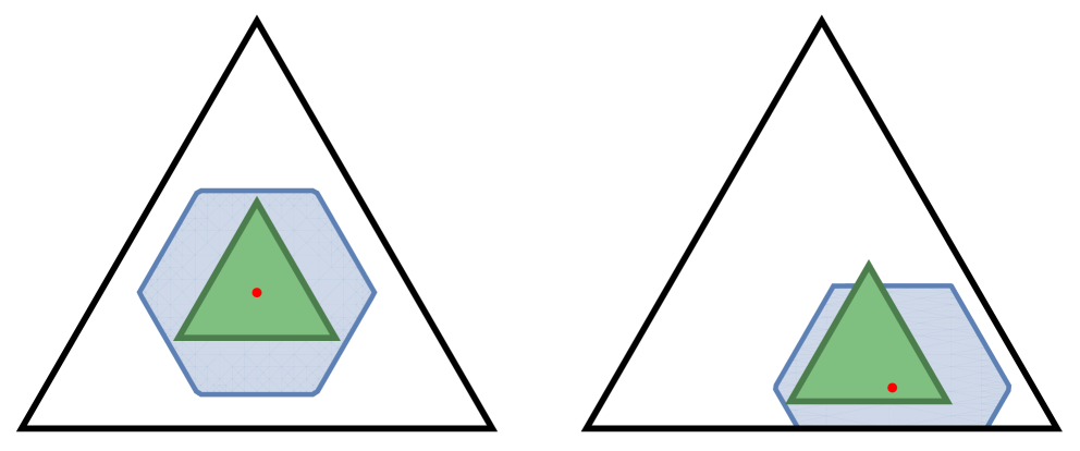
Figure 5: Normalized feasible sets $\frac{1}{1+\varepsilon}\mathcal{B}_{\varepsilon}(\mu)$ (green) and TV $\varepsilon$-balls (blue) centered at distinct points $\mu$ (red) in the 2-dimensional simplex. Our feasible sets with different centers are translations of each other, while the right TV ball interacts non-trivially with the simplex boundary.

To start, we apply Proposition 2 and invoke Kantorovich duality to obtain

$$\mathsf{W}_{p}^{\varepsilon}(\mu,\nu)^{p}=\inf_{\begin{subarray}{c}\mu^{\prime}\in\mathcal{B}_{\varepsilon}(\mu)\\ \nu^{\prime}\in\mathcal{B}_{\varepsilon}(\nu)\end{subarray}}\sup_{\begin{subarray}{c}\varphi,\psi\in C_{b}(\mathcal{X})\\ \varphi(x)+\psi(y)\leq\mathsf{d}(x,y)^{p}\>\forall x,y\end{subarray}}\mathopen{}\mathclose{{}\left[\int_{\mathcal{X}}\varphi\,\mathrm{d}\mu^{\prime}+\int_{\mathcal{X}}\varphi^{c}\,\mathrm{d}\nu^{\prime}}\right].$$

Since $\mathcal{X}$ is compact, it is straightforward to verify the conditions for the minimax theorem. Indeed: the feasible set for the infimum is convex and compact under the topology of weak convergence; the feasible set for the supremum is convex; and the objective is bilinear and continuous w.r.t. weak convergence of $\mu^{\prime}$ and $\nu^{\prime}$ and uniform convergence of $\varphi$ and $\psi$. Applying Sion’s minimax theorem and (9) gives

$$\mathsf{W}_{p}^{\varepsilon}(\mu,\nu)^{p} =\,\sup_{\begin{subarray}{c}\varphi,\psi\in C_{b}(\mathcal{X})\\ \varphi(x)+\psi(y)\leq\mathsf{d}(x,y)^{p}\end{subarray}}\mathopen{}\mathclose{{}\left[\inf_{\mu^{\prime}\in\mathcal{B}_{\varepsilon}(\mu)}\int_{\mathcal{X}}\varphi\,\mathrm{d}\mu^{\prime}+\inf_{\nu^{\prime}\in\mathcal{B}_{\varepsilon}(\nu)}\int_{\mathcal{X}}\psi\,\mathrm{d}\nu^{\prime}}\right]$$

$$=\,\sup_{\begin{subarray}{c}\varphi,\psi\in C_{b}(\mathcal{X})\\ \varphi(x)+\psi(y)\leq\mathsf{d}(x,y)^{p}\end{subarray}}\mathopen{}\mathclose{{}\left[\int_{\mathcal{X}}\varphi\,\mathrm{d}\mu+\int_{\mathcal{X}}\psi\,\mathrm{d}\nu+\varepsilon\mathopen{}\mathclose{{}\left(\inf_{x\in\mathcal{X}}\varphi(x)+\inf_{y\in\mathcal{X}}\psi(y)}\right)}\right].$$

We stress that if $\mu^{\prime}$ and $\nu^{\prime}$ instead varied within TV balls, the inner minimization problems would not admit closed forms due to boundary interactions.

Next, observe that replacing $\psi$ with $\varphi^{c}$ preserves feasibility. Indeed, $\varphi(x)+\varphi^{c}(y)\leq\mathsf{d}(x,y)^{p}$ by definition of the $c$-transform, and $\varphi^{c}$ is Lipschitz (and hence continuous) since

$$|\varphi^{c}(y)-\varphi^{c}(y^{\prime})|\leq\sup_{x\in\mathcal{X}}|\mathsf{d}(x,y)^{p}-\mathsf{d}(x,y^{\prime})^{p}|\leq p\operatorname{diam}(\mathcal{X})^{p-1}\mathsf{d}(y,y^{\prime}).$$

Moreover, this substitution can only increase the objective, so we have

$$\mathsf{W}_{p}^{\varepsilon}(\mu,\nu)^{p} =\,\sup_{\varphi\in C_{b}(\mathcal{X})}\mathopen{}\mathclose{{}\left[\int_{\mathcal{X}}\varphi\,\mathrm{d}\mu+\int_{\mathcal{X}}\varphi^{c}\,\mathrm{d}\nu+\varepsilon\mathopen{}\mathclose{{}\left(\inf_{x\in\mathcal{X}}\varphi(x)+\inf_{y\in\mathcal{X}}\varphi^{c}(y)}\right)}\right]$$

$$=\,\sup_{\varphi\in C_{b}(\mathcal{X})}\mathopen{}\mathclose{{}\left[\int_{\mathcal{X}}\varphi\,\mathrm{d}\mu+\int_{\mathcal{X}}\varphi^{c}\,\mathrm{d}\nu-\varepsilon\mathopen{}\mathclose{{}\left(\sup_{x\in\mathcal{X}}\varphi(x)-\inf_{x\in\mathcal{X}}\varphi(x)}\right)}\right],$$

where we have used the fact that $\inf_{y}\varphi^{c}(y)=\inf_{x,y}\mathsf{d}(x,y)^{p}-\varphi(x)=-\sup_{x}\varphi(x)$. The same reasoning allows us to restrict to $\varphi=(\varphi^{c})^{c}$ if desired. Since adding a constant to $\varphi$ decreases $\varphi^{c}$ by the same constant, we are free to shift $\varphi$ so that the final term equals $2\varepsilon\|\varphi\|_{\infty}$. Without shifting, we always have $\sup_{x}\varphi(x)-\inf_{x}\varphi(x)\leq 2\|\varphi\|_{\infty}$, so the problem simplifies to

$$\mathsf{W}_{p}^{\varepsilon}(\mu,\nu)^{p}=\,\sup_{\varphi\in C_{b}(\mathcal{X})}\int_{\mathcal{X}}\varphi\,\mathrm{d}\mu+\int_{\mathcal{X}}\varphi^{c}\,\mathrm{d}\nu-2\varepsilon\|\varphi\|_{\infty}.$$

For existence of maximizers, we first restrict the feasible set to those $\varphi$ with $\|\varphi\|_{\infty}\leq\mathsf{W}_{p}^{\varepsilon/2}(\mu,\nu)/\varepsilon$ (which is finite by Proposition 1). This is permissible since, for any $\varphi\in C_{b}(\mathcal{X})$ such that $\|\varphi\|_{\infty}>\mathsf{W}_{p}^{\varepsilon/2}(\mu,\nu)/\varepsilon$, we have

$$\int_{\mathcal{X}}\varphi\,\mathrm{d}\mu+\int_{\mathcal{X}}\varphi^{c}\,\mathrm{d}\nu-2\varepsilon\|\varphi\|_{\infty}\leq\mathsf{W}_{p}^{\varepsilon/2}(\mu,\nu)-\varepsilon\|\varphi\|_{\infty}<0\leq\mathsf{W}_{p}^{\varepsilon}(\mu,\nu).$$ (10)

Finally, the argument preceding Proposition 1.11 of Santambrogio (2015) implies that the restricted feasible set is uniformly equicontinuous. Since $\mathcal{X}$ is compact, Arzelà–Ascoli implies that the supremum is achieved. ∎

Remark 7 (TV as a dual norm).

Recall that $\|\cdot\|_{\mathsf{TV}}$ is the dual norm corresponding to the Banach space of measurable functions on $\mathcal{X}$ equipped with $\|\cdot\|_{\infty}$. An inspection of the proof of Proposition 4 reveals that our penalty scales with $\|\cdot\|_{\infty}$ precisely for this reason.

Lastly, we describe an alternative dual form which ties robust OT to loss trimming—a popular practical tool for robustifying estimation algorithms when $\mu$ and $\nu$ have finite support (Shen and Sanghavi, 2019).

[Loss trimming dual]propositionlosstrimming If $\mu,\nu\in\mathcal{P}(\mathcal{X})$ are uniform distributions over $n$ points each and $\varepsilon\in[0,1]$ is a multiple of $1/n$, then

$$\mathsf{W}_{p}^{\varepsilon}(\mu,\nu)^{p}=\sup_{\varphi\in C_{b}(\mathcal{X})}\mathopen{}\mathclose{{}\left(\min_{\begin{subarray}{c}\mathcal{A}\subseteq\operatorname{spt}(\mu)\\ |\mathcal{A}|=(1-\varepsilon)n\end{subarray}}\frac{1}{n}\sum_{x\in\mathcal{A}}\varphi(x)+\min_{\begin{subarray}{c}\mathcal{B}\subseteq\operatorname{spt}(\nu)\\ |\mathcal{B}|=(1-\varepsilon)n\end{subarray}}\frac{1}{n}\sum_{y\in\mathcal{B}}\varphi^{c}(y)}\right).$$

The inner minimization problems above clip out the $\varepsilon n$ fraction of samples whose potential evaluations are largest. This is similar to how standard loss trimming clips out a fraction of samples that contribute most to the considered training loss.

6 Experiments

To demonstrate the practical utility of the proposed robust OT framework, we outline the implementation of a scalable dual-based solver for $\mathsf{W}_{p}^{\varepsilon}$ and apply it to generative modeling experiments with contaminated data.

6.1 Computing $\bm{\mathsf{W}_{p}^{\varepsilon}}$ via its Dual Form

In practice, similarity between datasets is often measured using a so-called neural network (NN) distance $\mathsf{D}_{\mathrm{nn}}(\mu,\nu)=\sup_{\theta\in\Theta}\int f_{\theta}\,\mathrm{d}\mu-\int f_{\theta}\,\mathrm{d}\nu$, where $\{f_{\theta}\}_{\theta\in\Theta}\eqqcolon\mathcal{F}_{\mathrm{nn}}$ is a fixed NN class (Arora et al., 2017). Given two batches of samples $X_{1},\dots,X_{n}\sim\mu$ and $Y_{1},\dots,Y_{n}\sim\nu$, we approximate integrals by sample means and estimate the supremum via stochastic gradient ascent. Namely, we follow the update rule

$$\theta_{t+1}\leftarrow\theta_{t}+\frac{\alpha_{t}}{n}\sum_{i=1}^{n}\big{[}\nabla_{\theta}f_{\theta}(X_{i})-\nabla_{\theta}f_{\theta}(Y_{i})\big{]}.$$

When $\mathcal{F}_{\mathrm{nn}}$ approximates the class of 1-Lipschitz functions, we approach the Kantorovich dual and obtain an estimate of $\mathsf{W}_{1}(\mu,\nu)$, which is the core idea behind the WGAN (Arjovsky et al., 2017) (see Makkuva et al. (2020) for an extension to $\mathsf{W}_{2}$).

By virtue of our duality theory, OT solvers as described above can be easily adapted to the robust framework. For generative modeling, the one-sided robust distance defined by

$$\mathsf{W}_{p}^{\varepsilon}(\mu\|\nu)\coloneqq\inf_{\begin{subarray}{c}0\leq\mu^{\prime}\leq\mu\\ \mu^{\prime}(\mathcal{X})=1-\varepsilon\end{subarray}}\mathsf{W}_{p}\bigl{(}\mu,(1-\varepsilon)\nu\bigr{)}$$ (11)

is most appropriate, since data may be contaminated but generated samples from the model are not. In Section A.1, we translate our duality result from Proposition 4 to this setting, finding that

$$\begin{split}\mathsf{W}_{p}^{\varepsilon}(\mu\|\nu)^{p}=\sup_{\varphi\in C_{b}(\mathcal{X})}\int_{\mathcal{X}}\varphi\,\mathrm{d}\mu+(1-\varepsilon)\int_{\mathcal{X}}\varphi^{c}\,\mathrm{d}\nu-\varepsilon\sup_{x\in\mathcal{X}}\varphi(x).\end{split}$$ (12)

This representation suggests a modified gradient update for the corresponding NN distance estimate:

$$\theta_{t+1}\leftarrow\theta_{t}+\frac{\alpha_{t}}{n}\sum_{i=1}^{n}\big{[}\nabla_{\theta}f_{\theta}(X_{i})-(1-\varepsilon)\nabla_{\theta}f_{\theta}(Y_{i})\big{]}-\varepsilon\,\nabla_{\theta}f_{\theta}(X_{i^{*}}),\quad i^{*}\in\operatorname{argmax}_{i}f_{\theta}(X_{i}).$$

For example, in a PyTorch implementation of WGAN, the modified update can be implemented with a one-line adjustment of code:

⬇

score = f_data.mean() - f_generated.mean() # old

score = f_data.mean() - (1-eps)*f_generated.mean() - eps*f_data.max() # new

Due to the non-convex and non-smooth nature of the objective, formal optimization guarantees seem challenging to obtain, and we defer this exploration for future work. Nevertheless, this approach proves quite fruitful in practice, as we demonstrate next. Code for the results to follow is available at https://github.com/sbnietert/robust-OT, and full experimental details are provided in Section A.2. Computations were performed on a cluster machine equipped with a NVIDIA Tesla V100.

6.2 Generative Modeling with Contaminated Datasets

Robust GANs            Standard GANs

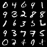
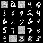
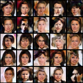
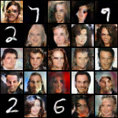
Figure 6: (top): samples generated by robustified (left) and standard (right) WGAN-GP after training on corrupted MNIST dataset. (bottom): samples generated by robustified (left) and standard (right) StyleGAN 2 after training on corrupted CelebA-HQ dataset (left).

We examine outlier-robust generative modeling using the modification suggested above. To that end, we trained two WGAN with gradient penalty (WGAN-GP) models (Gulrajani et al., 2017) on a contaminated dataset with 80% MNIST data and 20% uniform random noise. Both models used a standard selection of hyperparameters but one of them was adjusted to compute gradient updates according to the robust objective with $\varepsilon=0.25$. In Fig. 6 (top), we display generated samples produced by both networks after processing 125k contaminated batches of 64 images. The effect of outliers is clearly mitigated by training with the robustified objective.

capposition=beside,capbesideposition=top,right,capposition=bottom

Ours                 Balaji et al. (2020)   Staerman et al. (2021)            Control

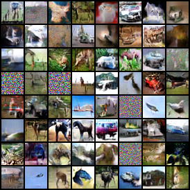
Figure 7: Samples generated by various robust GANs after 100k batches of training.

We also applied our robustification technique to more sophisticated generative models which incorporate additional regularization on top of WGAN. In particular, we trained two off-the-shelf StyleGAN 2 models (Karras et al., 2020) using contaminated data—this time, 80% CelebA-HQ face photos and 20% MNIST data—with one tweaked to perform gradient updates according to the robust objective with $\varepsilon=0.25$. We present generated samples in Fig. 6 (bottom). Once again, the modified objective enables learning a model that is largely free of outliers despite being trained on a contaminated dataset.

Finally, we compared our robust GAN approach with the existing techniques of Balaji et al. (2020) and Staerman et al. (2021). Using the publicly available code for these papers, we trained these robust GANs with their default options for 100k batches of 128 images, using 95% CIFAR-10 training images with 5% uniform random noise. In Fig. 7 and Table 1, the control GAN is that of Balaji et al. (2020) without its robustification weights enabled, and our robust GAN is obtained by adding the objective modification with $\varepsilon=0.07$ to this control. Fig. 7 presents random samples of generated images from the four GANs, while Table 1 displays Frechet inception distance (FID) scores (Heusel et al., 2017) over the course of training (lower scores correlate with high quality images). Our method performs favorably without tuning, but more detailed empirical study is needed to separate the impact of various hyperparameters. In particular, the poor relative performance of Staerman et al. (2021) is likely due in part to its distinct architecture. We also note that despite using the code provided by Balaji et al. (2020) with the hyperparameters specified in their appendix without any modification, the FID scores we observe in Table 1 are lower than those presented in their paper.

	Robust GAN Method
Batch	Ours	Balaji et al. (2020)	Staerman et al. (2021)	Control (Balaji et al., 2020)
20k	38.61	60.92	58.19	59.19
60k	22.08	35.49	49.64	39.08
100k	18.87	30.44	40.81	31.40

Table 1: FID scores between uncontaminated CIFAR-10 image dataset and datasets generated by various robust GANs during training.

7 Application to Sliced Optimal Transport

Finally, we extend the theory developed in this paper to projection-robust and sliced OT. These variants of the classic Wasserstein distance are obtained by taking either an average or maximum of $\mathsf{W}_{p}$ between lower-dimensional projections. Throughout, we fix $\mathcal{X}=\mathbb{R}^{d}$ and $k\in\{1,\dots,d\}$. Write $\mathrm{St_{k}(\mathbb{R}^{d})}\coloneqq\{U\in\mathbb{R}^{d\times k}:U^{\top}U=\mathrm{I}_{k}\}$ for the Stiefel manifold of orthonormal $k$-frames in $\mathbb{R}^{d}$ and $\sigma_{k}\in\mathcal{P}(\mathrm{St_{k}(\mathbb{R}^{d})})$ for its Haar measure. For $U\in\mathrm{St_{k}(\mathbb{R}^{d})}$, let $\mathfrak{p}^{U}:\mathbb{R}^{d}\to\mathbb{R}^{k}$ denote the corresponding projection mapping $\mathfrak{p}^{U}(x)\coloneqq U^{\top}x$. Also let $U_{k}\coloneqq(\mathrm{I}_{k}\>\>0_{d-k,d-k})^{\top}\in\mathrm{St_{k}(\mathbb{R}^{d})}$ be the standard projection matrix onto $\mathbb{R}^{k}$. We then define the $k$-dimensional average-sliced Wasserstein distance between $\mu,\nu\in\mathcal{P}(\mathbb{R}^{d})$ by

$$\underline{\mathsf{W}}_{p,k}(\mu,\nu)\coloneqq\left(\int_{\mathrm{St_{k}(\mathbb{R}^{d})}}\mathsf{W}_{p}\left(\mathfrak{p}^{U}_{\#}\mu,\mathfrak{p}^{U}_{\#}\nu\right)^{p}\,\mathrm{d}\sigma_{k}(U)\right)^{\frac{1}{p}},$$

and the $k$-dimensional max-sliced Wasserstein distance between them by

$$\overline{\mathsf{W}}_{p,k}(\mu,\nu)\coloneqq\sup_{U\in\mathrm{St_{k}(\mathbb{R}^{d})}}\mathsf{W}_{p}\left(\mathfrak{p}^{U}_{\#}\mu,\mathfrak{p}^{U}_{\#}\nu\right).$$

In the literature, “sliced OT” most typically refers to the setting where $k=1$, while “projection-robust OT” refers to our max-sliced definition. Both variants are metrics over $\mathcal{P}_{p}(\mathbb{R}^{d})$ which generate the same topology as classic $\mathsf{W}_{p}$ (Bonnotte, 2013; Nadjahi et al., 2019; Bayraktar and Guo, 2021; Nadjahi et al., 2020). Despite the name, formal outlier-robustness guarantees for either sliced distance were not presented until our preliminary work (Nietert et al., 2022). We now expand on this work by extending $\mathsf{W}_{p}^{\varepsilon}$ to the sliced setting. We start by setting up a unified framework of robust distribution estimation under sliced Wasserstein distances. Proofs are deferred to Appendix C.

Error and risk.

Fix a statistical distance $\mathsf{D}\in\{\underline{\mathsf{W}}_{p,k},\overline{\mathsf{W}}_{p,k}\}$ and family of clean distributions $\mathcal{G}\subseteq\mathcal{P}(\mathcal{X})$. Employing the $\varepsilon$-corruption model of Section 4, we seek an estimator $\mathsf{T}$ operating on contaminated samples which minimizes the $n$-sample risk

$$R_{n}(\mathsf{T},\mathsf{D},\mathcal{G},\varepsilon)\coloneqq\sup_{\mu\in\mathcal{G}}\inf\left\{\tau\geq 0:\sup_{\mathbb{P}_{n}\in\mathcal{M}_{n}^{\mathrm{adv}}(\mu,\varepsilon)}\mathbb{P}_{n}\Bigl{(}\mathsf{D}\bigl{(}\mathsf{T}(\tilde{\mu}_{n}),\mu\bigr{)}>\tau\Bigr{)}<\frac{1}{10}\right\}.$$

As before, we write $R_{n}(\mathsf{D},\mathcal{G},\varepsilon)\coloneqq\inf_{\mathsf{T}}R_{n}(\mathsf{T},\mathsf{D},\mathcal{G},\varepsilon)$ for the $n$-sample minimax risk.

The estimators.

We next define robust proxies of the average- and max-sliced distances, respectively, as:

$$\underline{\mathsf{W}}_{p,k}^{\varepsilon}(\mu,\nu) \coloneqq\left(\int_{\mathrm{St_{k}(\mathbb{R}^{d})}}\mathsf{W}_{p}^{\varepsilon}\left(\mathfrak{p}^{U}_{\#}\mu,\mathfrak{p}^{U}_{\#}\nu\right)^{p}\,\mathrm{d}\sigma_{k}(U)\right)^{\frac{1}{p}}$$

$$\overline{\mathsf{W}}_{p,k}^{\varepsilon}(\mu,\nu) \coloneqq\sup_{U\in\mathrm{St_{k}(\mathbb{R}^{d})}}\mathsf{W}_{p}^{\varepsilon}\left(\mathfrak{p}^{U}_{\#}\mu,\mathfrak{p}^{U}_{\#}\nu\right),$$

substituting $\mathsf{W}_{p}^{\varepsilon}$ for $\mathsf{W}_{p}$ in their definitions. To solve the estimation tasks, we again perform MDE, considering the minimum distance estimates

$$\mathsf{T}_{[\mathcal{G},\underline{\mathsf{W}}_{p,k}^{\varepsilon}]}(\tilde{\mu}_{n}) \in\operatorname{argmin}_{\nu\in\mathcal{G}}\underline{\mathsf{W}}_{p,k}^{\varepsilon}(\tilde{\mu}_{n},\nu)$$

$$\mathsf{T}_{[\mathcal{G},\overline{\mathsf{W}}_{p,k}^{\varepsilon}]}(\tilde{\mu}_{n}) \in\operatorname{argmin}_{\nu\in\mathcal{G}}\overline{\mathsf{W}}_{p,k}^{\varepsilon}(\tilde{\mu}_{n},\nu).$$

7.1 Robust Estimation Guarantees for Sliced $\bm{\mathsf{W}_{p}}$

We start by characterizing population-limit risk. For a distance $\mathsf{D}\in\{\underline{\mathsf{W}}_{p,k},\overline{\mathsf{W}}_{p,k}\}$, a clean family $\mathcal{G}\subseteq\mathcal{P}(\mathcal{X})$ and a map $\mathsf{T}:\mathcal{P}(\mathcal{X})\to\mathcal{P}(\mathcal{X})$, we again define

$$R_{\infty}(\mathsf{T},\mathsf{D},\mathcal{G},\varepsilon)\coloneqq\sup_{\begin{subarray}{c}\mu\in\mathcal{G},\,\tilde{\mu}\in\mathcal{P}(\mathcal{X})\\ \|\tilde{\mu}-\mu\|_{\mathsf{TV}}\leq\varepsilon\end{subarray}}\mathsf{D}\bigl{(}\mathsf{T}(\tilde{\mu}),\mu\bigr{)},$$

with corresponding minimax risk $R_{\infty}(\mathsf{D},\mathcal{G},\varepsilon)=\inf_{\mathsf{T}}R_{p,\infty}(\mathsf{T},\mathsf{D},\mathcal{G},\varepsilon)$. We can obtain tight bounds for this quantity in terms of the previously considered minimax risks.

Theorem 4 (Population-limit minimax risk for sliced $\mathsf{W}_{p}$).

Fix $0\leq\varepsilon\leq 0.49$, $q>p$, and $\mathcal{G}\in\{\mathcal{G}_{q}(\sigma),\mathcal{G}_{\mathrm{subG}}(\sigma),\mathcal{G}_{\mathrm{cov}}(\sigma)\}$ (assuming in the last case that $p<2$). Letting $\mathcal{G}_{k}\coloneqq\{\mathfrak{p}^{U_{k}}_{\#}\mu:\mu\in\mathcal{G}\}$ denote the orthogonal projection of $\mathcal{G}$ onto $\mathbb{R}^{k}$, we have

$$R_{\infty}(\underline{\mathsf{W}}_{p,k},\mathcal{G},\varepsilon) \asymp\sqrt{1\land\frac{k+p}{d}}\,R(\mathsf{W}_{p},\mathcal{G},\varepsilon),$$

$$R_{\infty}(\overline{\mathsf{W}}_{p,k},\mathcal{G},\varepsilon) \asymp R(\mathsf{W}_{p},\mathcal{G}_{k},\varepsilon),$$

and these risks are achieved by the estimators and $\mathsf{T}_{[\mathcal{G},\underline{\mathsf{W}}_{p,k}^{\varepsilon}]}$ and $\mathsf{T}_{[\mathcal{G},\overline{\mathsf{W}}_{p,k}^{\varepsilon}]}$, respectively (as well as by $\mathsf{T}_{[\mathcal{G},\|\cdot\|_{\mathsf{TV}}]}$ in both cases).

Specializing these bounds to each of the mentioned classes, we have the following corollary.

Corollary 2 (Concrete population-limit risk bounds).

For $0\leq\varepsilon\leq 0.49$, we have

$$R_{p}(\overline{\mathsf{W}}_{p,k},\mathcal{G},\varepsilon) \asymp\begin{cases}\sigma\varepsilon^{\frac{1}{p}-\frac{1}{q}},&\text{if $\mathcal{G}=\mathcal{G}_{q}(\sigma)$ for $q>p$}\\ \sigma\sqrt{k+p+\log\mathopen{}\mathclose{{}\left(\frac{1}{\varepsilon}}\right)}\,\varepsilon^{\frac{1}{p}},&\text{if $\mathcal{G}=\mathcal{G}_{\mathrm{subG}}(\sigma)$}\\ \sigma\sqrt{k}\,\varepsilon^{\frac{1}{p}-\frac{1}{2}},&\text{if $p<2$, and $\mathcal{G}=\mathcal{G}_{\mathrm{cov}}(\sigma)$}\\ \end{cases}$$

$$\vspace{5mm}R_{p}(\underline{\mathsf{W}}_{p,k},\mathcal{G},\varepsilon) \asymp\begin{cases}\sigma\sqrt{1\land\frac{k+p}{d}}\,\varepsilon^{\frac{1}{p}-\frac{1}{q}},&\text{if $\mathcal{G}=\mathcal{G}_{q}(\sigma)$ for $q>p$}\\ \sigma\sqrt{\mathopen{}\mathclose{{}\left(1\land\frac{k+p}{d}}\right)\mathopen{}\mathclose{{}\left(d+p+\log\mathopen{}\mathclose{{}\left(\frac{1}{\varepsilon}}\right)}\right)}\,\varepsilon^{\frac{1}{p}},&\text{if $\mathcal{G}=\mathcal{G}_{\mathrm{subG}}(\sigma)$}\\ \sigma\sqrt{k}\,\varepsilon^{\frac{1}{p}-\frac{1}{2}}.&\text{if $p<2$, and $\mathcal{G}=\mathcal{G}_{\mathrm{cov}}(\sigma)$}\\ \end{cases}$$

That is, average-sliced risks are proportional to standard risks with a multiplier of $\sqrt{k/d}$ when $d\gg p$, and max-sliced risks are equal to standard risks in $\mathbb{R}^{k}$. This extends Theorem 2 of Nietert et al. (2022) to general $k$ and a wider selection of clean families. Moreover, the proof is markedly simpler, connecting risks directly to those under classic $\mathsf{W}_{p}$. As before, our argument extends to a class of distributions with bounded Orlicz norm of a certain type, including those with bounded projected $q$th moments for $q>2$. For the upper bounds, we show that the modulus of continuity characterizing $\overline{\mathsf{W}}_{p,k}$ risk equals that of the $\mathsf{W}_{p}$ in $\mathbb{R}^{k}$, and that resilience w.r.t. $\underline{\mathsf{W}}_{p,k}$ is bounded by the same term appearing in the proof for $\mathsf{W}_{p}$ up to a prefactor of $O(\sqrt{1\land(k+p)/d})$. For the lower bounds, we are able to reuse examples constructed for Theorem 1.

We next provide near-tight risk bounds for the classes above in the finite-sample regime.

Theorem 5 (Finite-sample minimax risk for sliced $\mathsf{W}_{p}$).

Fix $0\leq\varepsilon\leq 0.49$, $q>p$, and $\mathcal{G}\in\{\mathcal{G}_{q}(\sigma),\mathcal{G}_{\mathrm{subG}}(\sigma),\mathcal{G}_{\mathrm{cov}}(\sigma)\}$ (assuming in the last case that $p<2$). Then, for $(\mathsf{D},\mathsf{D}^{\varepsilon})\in\{(\underline{\mathsf{W}}_{p,k},\underline{\mathsf{W}}_{p,k}^{\varepsilon}),(\overline{\mathsf{W}}_{p,k},\overline{\mathsf{W}}_{p,k}^{\varepsilon})\}$, we have

$$R_{\infty}(\mathsf{D},\mathcal{G},\varepsilon)+R_{n}(\mathsf{D},\mathcal{G},0)\lesssim R_{n}(\mathsf{D},\mathcal{G},\varepsilon)\lesssim R_{\infty}(\overline{\mathsf{W}}_{p,k},\mathcal{G},\varepsilon)+\sup_{\mu\in\mathcal{G}}\operatorname{\mathbb{E}}[\mathsf{D}(\hat{\mu}_{n},\mu)],$$

and the upper bound is achieved by the minimum distance estimator $\mathsf{T}_{[\mathcal{G},\mathsf{D}^{\varepsilon}]}$.

Remark 8 (Population-limit discrepancy for $\underline{\mathsf{W}}_{p,k}$).

Ideally, the population-limit term in the upper bound would be adapted to $\mathsf{D}$ rather than fixed to the larger max-sliced risk. However, the proof in Section C.2 relies on the max-sliced resilience of $\mathcal{G}$, and it is not clear whether $\mathsf{T}_{[\mathcal{G},\underline{\mathsf{W}}_{p,k}^{\varepsilon}]}$ can achieve this lower risk in general. For specific families $\mathcal{G}$, we may have $R_{\infty}(\overline{\mathsf{W}}_{p,k},\mathcal{G},\varepsilon)\asymp R_{\infty}(\underline{\mathsf{W}}_{p,k},\mathcal{G},\varepsilon)$, in which case this gap is negligible. For example, when $p=1$ and $\mathcal{G}=\mathcal{G}_{\mathrm{cov}}(\sigma)$, both risks are $\Theta(\sqrt{k\varepsilon})$.

For $\overline{\mathsf{W}}_{p,k}$, we match the population-limit risk up to empirical approximation error for the standard classes. In this case, the gap between the upper and lower bounds is simply the sub-optimality of plug-in estimation under $\overline{\mathsf{W}}_{p,k}$. For small $k$, we note that the empirical approximation error $\operatorname{\mathbb{E}}[\mathsf{D}(\hat{\mu}_{n},\mu)]$ can be significantly smaller than that under $\mathsf{W}_{p}$ (Lin et al., 2021; Niles-Weed and Rigollet, 2022) (see also (Nietert et al., 2022, Section 3)). Compared to the analogous results for $k=1$ in (Nietert et al., 2022), our results hold for all sample sizes $n$, and our proof is cleaner, following the approach of Theorem 2 via approximate triangle inequalities and appropriate modulus of continuity bounds. As was the case there, our argument also extends to approximate MDE.

Remark 9 (Average-sliced improvements).

Note that for the average-sliced Wasserstein distance, there is a gap between the upper and lower bounds in Theorem 5. In particular, the upper bound does not coincide with the population risk as $n\to\infty$. It remains unclear whether the finite-sample risk bound for MDE under $\underline{\mathsf{W}}_{p,k}^{\varepsilon}$ (or an alternative robustification of $\underline{\mathsf{W}}_{p,k}$) can be improved to $R_{\infty}(\underline{\mathsf{W}}_{p,k},\mathcal{G},\varepsilon)+\sup_{\mu\in\mathcal{G}}\operatorname{\mathbb{E}}[\mathsf{D}(\hat{\mu}_{n},\mu)]$, so that the first term matches the population-limit risk from Theorem 4 and the second is the current empirical convergence term from Theorem 5. We remark that Proposition 2 in Nietert et al. (2022) bridges this gap for $k=1$ via MDE under the TV norm, but the resulting bound contains a non-standard truncated empirical convergence term and only holds for sufficiently large sample sizes.

Next, we consider direct estimation of the sliced distances via their robust proxies.

Theorem 6 (Finite-sample robust estimation of sliced $\mathsf{W}_{p}$).

Let $0\leq\varepsilon<1/3$, write $\tau=1-(1-3\varepsilon)^{1/p}\in[3\varepsilon/p,3\varepsilon]$, and fix $(\mathsf{D},\mathsf{D}^{\varepsilon})\in\{(\underline{\mathsf{W}}_{p,k},\underline{\mathsf{W}}_{p,k}^{\varepsilon}),(\overline{\mathsf{W}}_{p,k},\overline{\mathsf{W}}_{p,k}^{\varepsilon})\}$. Let $\mu,\nu\in\mathcal{P}(\mathcal{X})$ be $(\rho,3\varepsilon)$-resilient w.r.t. $\overline{\mathsf{W}}_{p,k}$ with empirical measures $\hat{\mu}_{n}$ and $\hat{\nu}_{n}$, respectively. Then for any $\tilde{\mu}_{n},\tilde{\nu}_{n}\in\mathcal{P}(\mathcal{X})$ such that $\|\tilde{\mu}_{n}-\hat{\mu}_{n}\|_{\mathsf{TV}},\|\tilde{\nu}_{n}-\hat{\nu}_{n}\|_{\mathsf{TV}}\leq\varepsilon$, we have

$$\big{|}\mathsf{D}^{\varepsilon}(\tilde{\mu}_{n},\tilde{\nu}_{n})-\mathsf{D}(\mu,\nu)\big{|}\lesssim\rho+\tau\mathsf{D}(\mu,\nu)+\mathsf{D}(\mu,\hat{\mu}_{n})+\mathsf{D}(\nu,\hat{\nu}_{n}).$$

In particular, if $\varepsilon\leq 0.33$ and $\mu,\nu\in\mathcal{G}$ for $\mathcal{G}\in\{\mathcal{G}_{q}(\sigma),\mathcal{G}_{\mathrm{subG}}(\sigma),\mathcal{G}_{\mathrm{cov}}(\sigma)\}$, $q>p$, then $\rho$ can be replaced with $R_{\infty}(\mathsf{D},\mathcal{G},\varepsilon)$ in the bound above.

As with Theorem 3, the $\mathsf{W}_{p}^{\varepsilon}$ estimate suffers from additive estimation error $O(\rho)$ and multiplicative estimation error $O(\tau)$, matching the resilience-based guarantees of MDE when $\mathsf{W}_{p}(\mu,\nu)$ is sufficiently small and $n$ is sufficiently large.

Remark 10 (Dual forms for robust sliced $\mathsf{W}_{p}$).

For $\varepsilon\in(0,1]$ and $\mu,\nu\in\mathcal{P}(\mathcal{X})$, plugging in the $\mathsf{W}_{p}^{\varepsilon}$ dual into the definitions of the robust sliced distances gives

$$\underline{\mathsf{W}}_{p,k}^{\varepsilon}(\mu,\nu)^{p} =\int_{\mathrm{St_{k}(\mathbb{R}^{d})}}\left(\sup_{\begin{subarray}{c}f\in C_{b}(\mathbb{R}^{k})\end{subarray}}\int_{\mathbb{R}^{k}}f\,\mathrm{d}\mathfrak{p}^{U}_{\#}\mu+\int_{\mathbb{R}^{k}}f^{c}\,\mathrm{d}\mathfrak{p}^{U}_{\#}\nu-2\varepsilon\|f\|_{\infty}\right)\,\mathrm{d}\sigma_{k}(U)$$

$$\overline{\mathsf{W}}_{p,k}^{\varepsilon}(\mu,\nu)^{p} =\sup_{\begin{subarray}{c}U\in\mathrm{St_{k}(\mathbb{R}^{d})}\\ f\in C_{b}(\mathbb{R}^{k})\end{subarray}}\int_{\mathbb{R}^{k}}f\,\mathrm{d}\mathfrak{p}^{U}_{\#}\mu+\int_{\mathbb{R}^{k}}f^{c}\,\mathrm{d}\mathfrak{p}^{U}_{\#}\nu-2\varepsilon\|f\|_{\infty}.$$

8 Proofs

8.1 Proofs for Section 3

We start by reviewing some relevant facts regarding OT and couplings. In what follows, we define $c\mathcal{P}(\mathcal{X})\coloneqq\{\mu\in\mathcal{M}_{+}(\mathcal{X}):\mu(\mathcal{X})=c\}$ for $c\geq 0$.

Fact 1.

For $\mu,\nu\in\mathcal{P}(\mathcal{X})$, we have $\mathsf{W}_{p}(\mu,\nu)\leq\mathsf{W}_{p}(\mu-\mu\land\nu,\nu-\mu\land\nu).$

Proof.

For any $\pi\in\Pi(\mu-\mu\land\nu,\nu-\mu\land\nu)$, the joint distribution $\pi^{\prime}=(\operatorname{Id},\operatorname{Id})_{\#}(\mu\land\nu)+\pi$ is a coupling for $\mu$ and $\nu$ with $\|d\|_{L^{p}(\pi^{\prime})}=\|d\|_{L^{p}(\pi)}$. Hence, $\mathsf{W}_{p}(\mu,\nu)\leq\inf_{\pi\in\Pi(\mu-\mu\land\nu,\nu-\mu\land\nu)}\|d\|_{L^{p}(\pi)}=\mathsf{W}_{p}(\mu-\mu\land\nu,\nu-\mu\land\nu)$. ∎

Fact 2.

For $\mu_{1},\mu_{2},\nu\in\mathcal{M}_{+}(\mathcal{X})$ such that $(\mu_{1}+\mu_{2})(\mathcal{X})=\nu(\mathcal{X})$, any joint measure $\pi\in\Pi(\mu_{1}+\mu_{2},\nu)$ can be decomposed as $\pi=\pi_{\mu_{1},\nu}+\pi_{\mu_{2},\nu}$ for $\pi_{\mu_{1},\nu},\pi_{\mu_{2},\nu}\in\mathcal{M}_{+}(\mathcal{X}^{2})$ such that $\mu_{1}(A)=\pi_{\mu_{1},\nu}(A\times\mathcal{X})$ and $\mu_{2}(A)=\pi_{\mu_{2},\nu}(A\times\mathcal{X})$ for all measurable $A\subseteq\mathcal{X}$.

Proof.

Write $\pi(y|x)$ for the regular conditional probability measure such that $\pi(A\times B)=\int_{A}\pi(B|x)\,\mathrm{d}(\mu_{1}+\mu_{2})(x)$ for all measurable $A,B\subseteq\mathcal{X}$. Then $\pi_{\mu_{1},\nu},\pi_{\mu_{2},\nu}\in\mathcal{M}(\mathcal{X}^{2})$ defined by

$$\pi_{\mu_{1},\nu}(A\times B)\coloneqq\int_{A}\pi(B|x)\,\mathrm{d}\mu_{1}(x)\quad\text{and}\quad\pi_{\mu_{2},\nu}(A\times B)\coloneqq\int_{A}\pi(B|x)\,\mathrm{d}\mu_{2}(x)$$

sum to $\pi$ and satisfy $\pi_{\mu_{1},\nu}(A\times\mathcal{X})=\int_{A}\pi(\mathcal{X}|x)\,\mathrm{d}\mu_{1}(x)=\mu_{1}(A)$ and $\pi_{\mu_{2},\nu}(A\times\mathcal{X})=\mu_{2}(A)$. ∎

8.1.1 Proof of Proposition 1

Let $\mu,\nu\in\mathcal{P}(\mathcal{X})$ and $0<\varepsilon_{1}\leq\varepsilon_{2}<\|\mu-\nu\|_{\mathsf{TV}}$ as in the proposition statement. Since $\mathcal{X}$ is a Polish space, $\mu$ and $\nu$ are tight; in particular, there is a compact set $K\subseteq\mathcal{X}$ such that $\mu(K),\nu(K)\geq 1-\varepsilon_{1}$. Letting $\mu^{\prime}=\frac{1-\varepsilon_{1}}{\mu(K)}\mu|_{K}$ and $\nu^{\prime}=\frac{1-\varepsilon_{1}}{\nu(K)}\nu|_{K}$, we have

$$\mathsf{W}_{p}^{\varepsilon_{1}}(\mu,\nu)\leq\mathsf{W}_{p}(\mu^{\prime},\nu^{\prime})\leq\operatorname{diam}(K)<\infty.$$

Now, fix any $\bar{\mu},\bar{\nu}\in(1-\varepsilon_{1})\mathcal{P}(\mathcal{X})$ feasible for the $\mathsf{W}_{p}^{\varepsilon_{1}}(\mu,\nu)$ problem. Letting $\bar{\mu}^{\prime}=\frac{1-\varepsilon_{2}}{1-\varepsilon_{1}}\bar{\mu}$ and $\bar{\nu}^{\prime}=\frac{1-\varepsilon_{2}}{1-\varepsilon_{1}}\bar{\nu}$, we have

$$\mathsf{W}_{p}^{\varepsilon_{2}}(\mu,\nu)\leq\mathsf{W}_{p}(\bar{\mu}^{\prime},\bar{\nu}^{\prime})=\mathopen{}\mathclose{{}\left(\frac{1-\varepsilon_{2}}{1-\varepsilon_{1}}}\right)^{\!\frac{1}{p}}\mathsf{W}_{p}(\bar{\mu},\bar{\nu}).$$

Infimizing over $\bar{\mu}$ and $\bar{\nu}$ gives $\mathsf{W}_{p}^{\varepsilon_{2}}(\mu,\nu)\leq\bigl{(}\frac{1-\varepsilon_{2}}{1-\varepsilon_{1}}\bigr{)}^{1/p}\mathsf{W}_{p}^{\varepsilon_{1}}(\mu,\nu)$. Next, we note that ${\|\mu-\nu\|_{\mathsf{TV}}}\leq\varepsilon_{2}$ if and only if there exists $\kappa\in(1-\varepsilon_{2})\mathcal{P}(\mathcal{X})$ with $\kappa\leq\mu$ and $\kappa\leq\nu$, which occurs if and only if $\mathsf{W}_{p}^{\varepsilon_{2}}(\mu,\nu)=0$. Finally, $\mathsf{W}_{p}^{0}(\mu,\nu)$ trivially coincides with $\mathsf{W}_{p}(\mu,\nu)$ since the only feasible measures for the $\mathsf{W}_{p}^{0}(\mu,\nu)$ problem are $\mu$ and $\nu$ themselves. ∎

8.1.2 Proof of Proposition 2

Denote the mass addition formulation by $\overline{\mathsf{W}}\vphantom{W}^{\varepsilon}_{p}(\mu,\nu)$. We first prove that $\mathsf{W}_{p}^{\varepsilon}(\mu,\nu)\geq\overline{\mathsf{W}}\vphantom{W}^{\varepsilon}_{p}(\mu,\nu)$. To see this, take any $\mu^{\prime}\leq\mu$ and $\nu^{\prime}\leq\nu$ with $\mu^{\prime}(\mathcal{X})=\nu^{\prime}(\mathcal{X})=1-\varepsilon$ feasible for the $\mathsf{W}_{p}^{\varepsilon}(\mu,\nu)$ problem. Then, we have that $\bar{\mu}^{\prime}=\mu+\nu-\nu^{\prime}$ and $\bar{\nu}^{\prime}=\nu+\mu-\mu^{\prime}$ are feasible for the $\overline{\mathsf{W}}\vphantom{W}^{\varepsilon}_{p}$ problem, and so

$$\overline{\mathsf{W}}\vphantom{W}^{\varepsilon}_{p}(\mu,\nu)\leq\mathsf{W}_{p}(\mu+\nu-\nu^{\prime},\nu+\mu-\mu^{\prime})\leq\mathsf{W}_{p}(\mu^{\prime},\nu^{\prime}),$$

where the final inequality uses 1.

For the opposite inequality, consider any $\mu^{\prime}\geq\mu$ and $\nu^{\prime}\geq\nu$ feasible for the $\overline{\mathsf{W}}\vphantom{W}^{\varepsilon}_{p}(\mu,\nu)$ problem, and write $\alpha=\mu^{\prime}-\mu$ and $\beta=\nu^{\prime}-\nu$. Taking $\pi\in\Pi(\mu^{\prime},\nu^{\prime})$ to be an optimal coupling for $\mathsf{W}_{p}(\mu^{\prime},\nu^{\prime})$, we apply 2 repeatedly to obtain a decomposition $\pi=\pi_{\mu,\nu}+\pi_{\mu,\beta}+\pi_{\alpha,\nu}+\pi_{\alpha,\beta}$ of $\pi$ into non-negative joint measures such that $\mu=(\pi_{\mu,\nu}+\pi_{\mu,\beta})(\cdot\times\mathcal{X})$, $\nu=(\pi_{\mu,\nu}+\pi_{\alpha,\nu})(\mathcal{X}\times\cdot)$, $\alpha=(\pi_{\alpha,\nu}+\pi_{\alpha,\beta})(\cdot\times\mathcal{X})$, and $\beta=(\pi_{\mu,\beta}+\pi_{\alpha,\beta})(\mathcal{X}\times\cdot)$. Consequently, we have

$$\pi_{\mu,\nu}(\mathcal{X}^{2})=(\pi_{\mu,\nu}+\pi_{\mu,\beta})(\mathcal{X}^{2})-\pi_{\mu,\beta}(\mathcal{X}^{2})\geq 1-\beta(\mathcal{X})=1-\varepsilon.$$

Defining normalized marginals $\tilde{\mu}^{\prime}$ and $\tilde{\nu}^{\prime}$ of $\pi_{\mu,\nu}$ by $\tilde{\mu}^{\prime}=\pi_{\mu,\nu}(\cdot\times\mathcal{X})\frac{1-\varepsilon}{\pi_{\mu,\nu}(\mathcal{X}^{2})}$ and $\tilde{\nu}^{\prime}=\pi_{\mu,\nu}(\mathcal{X}\times\cdot)\frac{1-\varepsilon}{\pi_{\mu,\nu}(\mathcal{X}^{2})}$, we observe that this pair is feasible for the $\mathsf{W}_{p}^{\varepsilon}(\mu,\nu)$ problem, i.e., $\tilde{\mu}^{\prime}\leq\mu$ and $\tilde{\nu}^{\prime}\leq\nu$ with $\tilde{\mu}^{\prime}(\mathcal{X})=\tilde{\nu}^{\prime}(\mathcal{X})=1-\varepsilon$. Hence, we have

$$\mathsf{W}_{p}^{\varepsilon}(\mu,\nu)^{p}\leq\mathsf{W}_{p}(\tilde{\mu}^{\prime},\tilde{\nu}^{\prime})^{p}\leq\|\mathsf{d}\|_{L^{p}(\pi_{\mu,\nu})}^{p}\frac{1-\varepsilon}{\pi_{\mu,\nu}(\mathcal{X}^{2})}\leq\|\mathsf{d}\|_{L^{p}(\pi_{\mu,\nu})}^{p}\leq\|\mathsf{d}\|_{L^{p}(\pi)}^{p}=\mathsf{W}_{p}(\mu^{\prime},\nu^{\prime}).$$

Taking an infimum over $\mu^{\prime},\nu^{\prime}$ feasible for $\overline{\mathsf{W}}\vphantom{W}^{\varepsilon}_{p}(\mu,\nu)$, we find that $\mathsf{W}_{p}^{\varepsilon}(\mu,\nu)\leq\overline{\mathsf{W}}\vphantom{W}^{\varepsilon}_{p}(\mu,\nu)$. Thus, we have $\mathsf{W}_{p}^{\varepsilon}(\mu,\nu)=\overline{\mathsf{W}}\vphantom{W}^{\varepsilon}_{p}(\mu,\nu)$, as desired. ∎

Remark 11 (General costs).

Observe that the argument above applies to the analogous mass removal and mass addition problems associated with the general OT cost $\mathsf{OT}_{c}$, so long as the base cost $c:\mathcal{X}^{2}\to[0,\infty)$ satisfies $c(x,x)=0$ for all $x\in\mathcal{X}$.

8.1.3 Proof of Proposition 3

It remains to prove the two lemmas needed for implications (3) and (5) in Fig. 2. We depict these results in Fig. 8 using the same diagram format as the sketch.

Figure 8: Diagrams illustrating Lemma 4 (left) and Lemma 5 (right).

Lemma 4.

Fix $\mu,\nu\in\mathcal{M}_{+}(\mathcal{X})$. Then for any $\alpha\in\mathcal{M}_{+}(\mathcal{X})$ with $\mu(\mathcal{X})=\alpha(\mathcal{X})$, there exists $\beta\in\mathcal{M}_{+}(\mathcal{X})$ with $\beta(\mathcal{X})=\nu(\mathcal{X})$ such that $\mathsf{W}_{p}(\beta,\nu)\leq\mathsf{W}_{p}(\mu,\alpha)$ and $\|\beta-\mu\|_{\mathsf{TV}}\leq\|\nu-\alpha\|_{\mathsf{TV}}$.

Proof.

Decompose $\nu=\alpha+\kappa_{+}-\kappa_{-}$ for $\kappa_{+},\kappa_{-}\in\mathcal{M}_{+}(\mathcal{X})$ such that $\kappa_{+}(\mathcal{X})+\kappa_{-}(\mathcal{X})=2\|\nu-\alpha\|_{\mathsf{TV}}$ and $\kappa_{-}\leq\alpha$, and let $\pi\in\Pi(\mu,\alpha)$ be an optimal coupling for $\mathsf{W}_{p}(\mu,\alpha)$. By 2, we can decompose $\pi=\pi_{1}+\pi_{2}$ for $\pi_{1},\pi_{2}\in\mathcal{M}_{+}(\mathcal{X}^{2})$ such that $\kappa_{-}=\pi_{1}(\mathcal{X}\times\cdot)$ and $\alpha-\kappa_{-}=\pi_{2}(\mathcal{X}\times\cdot)$. Define $\mu_{-}\in\mathcal{M}_{+}(\mathcal{X})$ with $\mu_{-}\leq\mu$ as the marginal of $\pi_{1}$ in its first coordinate, i.e., $\mu_{-}\coloneqq\pi_{1}(\cdot\times\mathcal{X})$. Now we consider $\beta\coloneqq\mu-\mu_{-}+\kappa_{+}\in\mathcal{M}_{+}(\mathcal{X})$ and the joint measure $\pi^{\prime}=\pi_{2}+(\operatorname{Id},\operatorname{Id})_{\#}\kappa_{+}\in\mathcal{M}_{+}(\mathcal{X}^{2})$. With these definitions, we obtain

$$\|\beta-\mu\|_{\mathsf{TV}} =\|\mu_{-}-\kappa_{+}\|_{\mathsf{TV}}$$

$$\leq\|\mu_{-}\|_{\mathsf{TV}}+\|\kappa_{+}\|_{\mathsf{TV}}$$

$$=2\kappa_{-}(\mathcal{X})+2\kappa_{+}(\mathcal{X})$$

$$=\|\nu-\alpha\|_{\mathsf{TV}}.$$

Moreover, for all measurable $A\subseteq\mathcal{X}$, we have

$$\pi^{\prime}(A\times\mathcal{X}) =\pi_{2}(A\times\mathcal{X})+\kappa_{+}(A)$$

$$=(\pi-\pi_{1})(A\times\mathcal{X})+\kappa_{+}(A)$$

$$=(\mu-\mu_{-}+\kappa_{+})(A)$$

$$=\beta(A)$$

and

$$\pi^{\prime}(\mathcal{X}\times A) =\pi_{2}(\mathcal{X}\times A)+\kappa_{+}(A)=(\alpha-\kappa_{-}+\kappa_{+})(A)=\nu(A).$$

Hence, $\pi^{\prime}\in\Pi(\beta,\nu)$, and so

$$\mathsf{W}_{p}(\beta,\nu)^{p}\leq\int_{\mathcal{X}}\mathsf{d}^{p}\,\mathrm{d}\pi^{\prime}=\int_{\mathcal{X}}\mathsf{d}^{p}\,\mathrm{d}\pi_{2}\leq\int_{\mathcal{X}}\mathsf{d}^{p}\,\mathrm{d}\pi=\mathsf{W}_{p}(\mu,\alpha)^{p},$$

as desired. ∎

Lemma 5.

Let $\mu,\nu\in\mathcal{M}_{+}(\mathcal{X})$ be such that $\mu(\mathcal{X})=\nu(\mathcal{X})$. For any $\alpha,\beta\in\mathcal{M}_{+}(\mathcal{X})$ such that $\alpha(\mathcal{X})=\beta(\mathcal{X})<\mu(\mathcal{X})$, there exist $\alpha^{\prime},\beta^{\prime}\in\mathcal{M}(\mathcal{X})$ that satisfy $\alpha^{\prime}\leq\mu$, $\beta^{\prime}\leq\nu$, $\|\alpha^{\prime}-\mu\|_{\mathsf{TV}},\|\beta^{\prime}-\nu\|_{\mathsf{TV}}\leq\|\alpha-\mu\|_{\mathsf{TV}}\lor\|\beta-\nu\|_{\mathsf{TV}}$, and $\mathsf{W}_{p}(\alpha^{\prime},\beta^{\prime})\leq\mathsf{W}_{p}(\alpha,\beta)$.

Proof.

Assume without generality that $\|\alpha-\mu\|_{\mathsf{TV}}\leq\|\beta-\nu\|_{\mathsf{TV}}$. Decompose $\alpha=\mu+\kappa_{+}-\kappa_{-}$ and $\beta=\nu+\lambda_{+}-\lambda_{-}$, for $\kappa_{+},\kappa_{-},\lambda_{+},\lambda_{-}\in\mathcal{M}_{+}(\mathcal{X})$ such that $\kappa_{+}(\mathcal{X})=\lambda_{+}(\mathcal{X})$ and $\kappa_{-}(\mathcal{X})=\lambda_{-}(\mathcal{X})$, where $\lambda_{-}(\mathcal{X})+\lambda_{+}(\mathcal{X})=2\|\beta-\nu\|_{\mathsf{TV}}$. Let $\pi\in\Pi(\alpha,\beta)$ be an optimal coupling for the $\mathsf{W}_{p}(\alpha,\beta)$ problem. Defining $\alpha_{+}\coloneqq\mu+\kappa_{+}+\lambda_{-}$, $\beta_{+}\coloneqq\nu+\lambda_{+}+\kappa_{-}$, and $\pi_{+}=\pi+(\operatorname{Id},\operatorname{Id})_{\#}(\kappa_{-}+\lambda_{-})\in\Pi(\alpha_{+},\beta_{+})$, we have $\alpha$

$$\mathsf{W}_{p}(\alpha_{+},\beta_{+})^{p}\leq\int_{\mathcal{X}}\mathsf{d}^{p}\,\mathrm{d}\pi_{+}=\int_{\mathcal{X}}\mathsf{d}^{p}\,\mathrm{d}\pi=\mathsf{W}_{p}(\alpha,\beta)^{p},$$

as desired. Since $\alpha_{+}$ and $\beta_{+}$ are feasible for the mass addition formulation of $\mathsf{W}_{p}^{\varepsilon}(\mu,\nu)$ with $\varepsilon=2\|\beta-\nu\|_{\mathsf{TV}}$, Proposition 2 implies that $\mathsf{W}_{p}^{\varepsilon}(\mu,\nu)\leq\mathsf{W}_{p}(\alpha,\beta)$. The lemma follows provided that the infimum defining $\mathsf{W}_{p}^{\varepsilon}$ is achieved, which we establish in the proof of Proposition 5. ∎

Given these results, the sketch in Section 3 is complete.∎

8.1.4 Proof of Proposition 5

We first prove existence of minimizers via a compactness argument, and then show that they can be taken to be bounded from below by $\mu\land\nu$. The latter step is simpler to prove in the discrete case, so we begin there and extend to the general case via a discretization argument.

Existence:

Because measures in the feasible set are positive and bounded from above by $\mu$ and $\nu$, the set is tight, i.e., pre-compact w.r.t. the topology of weak convergence. Moreover, the feasible set is closed w.r.t. this topology since it can be written as the intersection of the closed sets $\{(\mu^{\prime},\nu^{\prime})\in(1-\varepsilon)\mathcal{P}(\mathcal{X})^{2}:\mu^{\prime}(A)\leq\mu(A),\nu^{\prime}(A)\leq\nu(A)\}$ over all measurable $A\subseteq\mathcal{X}$. Hence, the feasible set is compact. Finally, $\mathsf{W}_{p}$ is lower-semicontinuous under the weak topology, i.e., if $\mu^{\prime}_{n}\stackrel{{\scriptstyle w}}{{\to}}\mu^{\prime}$ and $\nu^{\prime}_{n}\stackrel{{\scriptstyle w}}{{\to}}\nu^{\prime}$, then $\liminf_{n\to\infty}\mathsf{W}_{p}(\mu^{\prime}_{n},\nu^{\prime}_{n})\geq\mathsf{W}_{p}(\mu^{\prime},\nu^{\prime})$ (see, e.g., Villani (2009, Remark 6.10)). The infimum of a lower semicontinuous function over a compact set is always achieved, as desired.

Lower envelope (discrete case):

Having proven the existence of minimizers $\mu^{\prime}\leq\mu$ and $\nu^{\prime}\leq\nu$, it remains to show that we can take $\mu^{\prime},\nu^{\prime}\geq\mu\land\nu$. We begin with the discrete case where $\mathcal{X}$ is countable and treat measures and their mass functions interchangeably. Then, if $\mu^{\prime}\geq\mu\land\nu$ fails to hold, there exists $x_{0}\in\mathcal{X}$ such that $\mu^{\prime}(x_{0})<\mu(x_{0})$ and $\mu^{\prime}(x_{0})<\nu(x_{0})$. We can further assume that $\nu(x_{0})=\nu^{\prime}(x_{0})$. Otherwise, $a\coloneqq(\nu-\nu^{\prime})(x_{0})\land(\mu-\mu^{\prime})(x_{0})$ mass could be returned to both $\mu^{\prime}$ and $\nu^{\prime}$ at $x_{0}$ without increasing their transport cost. Indeed, for any $\pi\in\Pi(\mu^{\prime},\nu^{\prime})$, the modified plan $\pi+a\delta_{(x_{0},x_{0})}$ is valid for the new measures, $\mu^{\prime}+a\delta_{x_{0}}$ and $\nu^{\prime}+a\delta_{x_{0}}$ (still feasible by the choice of $a$), and attains the same cost.

Taking $\pi\in\Pi(\mu^{\prime},\nu^{\prime})$ optimal for $\mathsf{W}_{p}(\mu^{\prime},\nu^{\prime})$, we define the measure $\kappa\leq\mu^{\prime}$ by $\kappa(x_{0})=0$, $\kappa(x)=\pi(x,x_{0})$ for $x\neq x_{0}$. This captures the distribution of the mass that is transported away from $x_{0}$ w.r.t. $\pi$ when transporting $\nu^{\prime}$ to $\mu^{\prime}$. By conservation of mass, $\kappa$ has total mass at least $(\nu^{\prime}-\mu^{\prime})(x_{0})>0$, so we can set $\tilde{\kappa}\leq\kappa$ to be a scaled-down copy of $\kappa$ with total mass $(\mu\land\nu^{\prime}-\mu^{\prime})(x_{0})>0$. Now, define an alternative perturbed measure $\tilde{\mu}^{\prime}\coloneqq\mu^{\prime}+\tilde{\kappa}(\mathcal{X})\delta_{x_{0}}-\tilde{\kappa}$. By definition, we have $0\leq\tilde{\mu}^{\prime}\leq\mu$ with $\tilde{\mu}^{\prime}(\mathcal{X})=\mu^{\prime}(\mathcal{X})=1-\varepsilon$ and $\tilde{\mu}^{\prime}(x_{0})=(\mu\land\nu^{\prime})(x_{0})$. Furthermore, the modified plan $\tilde{\pi}\in\Pi(\tilde{\mu}^{\prime},\nu^{\prime})$ defined by

$$\tilde{\pi}(x,y)=\begin{cases}\pi(x,y),&y\neq x_{0}\\ \frac{\kappa(\mathcal{X})-\tilde{\kappa}(\mathcal{X})}{\kappa(\mathcal{X})}\pi(x,x_{0}),&x\neq x_{0},y=x_{0}\\ \pi(x_{0},x_{0})+\tilde{\kappa}(\mathcal{X}),&x=y=x_{0}\end{cases}$$

satisfies $\|\mathsf{d}\|_{L^{p}(\tilde{\pi})}<\|\mathsf{d}\|_{L^{p}(\pi)}=\mathsf{W}_{p}(\mu^{\prime},\nu^{\prime})$, contradicting optimality of $(\mu^{\prime},\nu^{\prime})$.

Lower envelope (general case):

For general $\mathcal{X}$, we will need the following lemma, which allows us to apply our discretization argument to our setting.

Lemma 6 (Dense approximation).

Let $(\mathcal{Y},\rho)$ be an (extended) metric space with dense subset $D\subseteq\mathcal{Y}$. For each $\lambda>0$, suppose we have an embedding $\mathcal{Y}\ni y\mapsto y^{\lambda}\in D$, such that $\rho(y,y^{\lambda})\leq\lambda$ for all $y\in\mathcal{Y}$. For any $K\subseteq\mathcal{Y}$, define $K^{\lambda}\coloneqq\{y^{\lambda}:y\in K\}$. If $f:\mathcal{Y}\to\mathbb{R}$ is uniformly continuous, then $\inf_{y\in K}f(y)=\lim_{\lambda\to 0}\inf_{y\in K^{\lambda}}f(y)$.

Proof.

As $\lambda\to 0$, we have

$$\Bigl{|}\inf_{y\in K}f(y)-\inf_{y\in K^{\lambda}}f(y)\Bigr{|}\leq\sup_{y\in K}\bigl{|}f(y)-f(y^{\lambda})\bigr{|}\leq\sup_{\begin{subarray}{c}y,y^{\prime}\in K\\ \rho(y,y^{\prime})\leq\lambda\end{subarray}}\bigl{|}f(y)-f(y^{\prime})\bigr{|}\to 0.\qed$$

We will essentially apply this lemma to the space of measures $\mathcal{Y}=(1-\varepsilon)\mathcal{P}(\mathcal{X})$ under $\mathsf{W}_{p}$, letting $D$ be its dense subset of discrete measures. For any $\lambda>0$, separability of $\mathcal{X}$ implies the existence of a countable partition $\{A_{i}^{\lambda}\}_{i\in\mathbb{N}}$ of $\mathcal{X}$ such that $\operatorname{diam}(A_{i}^{\lambda})\leq\lambda$ for all $i\in\mathbb{N}$, with representatives $x_{i}^{\lambda}\in A_{i}^{\lambda}$. For any measure $\kappa\in\mathcal{Y}$, we let $\kappa^{\lambda}\in\mathcal{M}_{+}(\{x_{i}^{\lambda}\}_{i\in\mathbb{N}})$ denote the discretized measure defined by $\kappa^{\lambda}\coloneqq\sum_{i\in\mathbb{N}}\kappa(A_{i}^{\lambda})\cdot\delta_{x_{i}^{\lambda}}$. We then have

$$\mathsf{W}_{p}(\kappa,\kappa^{\lambda})^{p}\leq\sum_{i\in\mathbb{N}}\mathsf{W}_{p}\bigl{(}\kappa|_{A_{i}^{\lambda}},\kappa(A_{i}^{\lambda})\cdot\delta_{x_{i}^{\lambda}}\bigr{)}^{p}\leq\sum_{i\in\mathbb{N}}\kappa(A_{i}^{\lambda})\lambda^{p}=\lambda^{p},$$

and so $\mathsf{W}_{p}(\kappa,\kappa^{\lambda})\leq\lambda$. This discretization lifts to sets of measures as in the lemma. Now, for any $\alpha,\beta\in\mathcal{M}_{+}(\mathcal{X})$ with $\alpha\leq\beta$, let $K_{\alpha,\beta}=\{\kappa\in\mathcal{Y}:\alpha\leq\kappa\leq\beta,\kappa(\mathcal{X})=1-\varepsilon\}$. Importantly, this choice of discretization satisfies $K_{\alpha,\beta}^{\lambda}=K_{\alpha^{\lambda},\beta^{\lambda}}$. Indeed if $\kappa\in K_{\alpha,\beta}$, then $\kappa^{\lambda}\in K_{\alpha^{\lambda},\beta^{\lambda}}$ by our discretization definition, and total mass is preserved. Likewise, if $\kappa\in K_{\alpha^{\lambda},\beta^{\lambda}}$, then we can consider

$$\tilde{\kappa}\coloneqq\sum_{i:x_{i}\in\operatorname{spt}(\kappa^{\prime})}\alpha|_{A_{i}^{\lambda}}+c_{i}(\beta-\alpha)|_{A_{i}^{\lambda}},$$

where $c_{i}\in[0,1]$ are chosen such that $\tilde{\kappa}(\{i\})=\kappa(A_{i})$ for all $i\in\mathbb{N}$. By this construction, we have $\kappa=\tilde{\kappa}^{\lambda}$ and $\tilde{\kappa}\in K_{\alpha,\beta}$ with $\tilde{\kappa}(\mathcal{X})=\kappa(\mathcal{X})=1-\varepsilon$, as desired. Also observe that $\alpha^{\lambda}\land\beta^{\lambda}=(\alpha\land\beta)^{\lambda}$.

Putting everything together, we finally obtain

$$\mathsf{W}_{p}^{\varepsilon}(\mu,\nu) =\inf_{\begin{subarray}{c}\mu^{\prime}\in K_{0,\mu}\\ \nu^{\prime}\in K_{0,\nu}\end{subarray}}\mathsf{W}_{p}(\mu^{\prime},\nu^{\prime}) \mathsf{W}_{p}^{\varepsilon}$$ (definition of )

$$=\lim_{\lambda\to 0}\inf_{\begin{subarray}{c}\mu^{\prime}\in K_{0,\mu}^{\lambda}\\ \nu^{\prime}\in K_{0,\nu}^{\lambda}\end{subarray}}\mathsf{W}_{p}(\mu^{\prime},\nu^{\prime})$$ (Lemma 6)

$$=\lim_{\lambda\to 0}\inf_{\begin{subarray}{c}\mu^{\prime}\in K_{0,\mu^{\lambda}}\\ \nu^{\prime}\in K_{0,\nu^{\lambda}}\end{subarray}}\mathsf{W}_{p}(\mu^{\prime},\nu^{\prime}) K_{\alpha,\beta}^{\lambda}=K_{a^{\lambda},b^{\lambda}}$$ ()

$$=\lim_{\lambda\to 0}\inf_{\begin{subarray}{c}\mu^{\prime}\in K_{\mu^{\lambda}\land\nu^{\lambda},\mu^{\lambda}}\\ \nu^{\prime}\in K_{\mu^{\lambda}\land\nu^{\lambda},\nu^{\lambda}}\end{subarray}}\mathsf{W}_{p}(\mu^{\prime},\nu^{\prime})$$ (discrete case)

$$=\lim_{\lambda\to 0}\inf_{\begin{subarray}{c}\mu^{\prime}\in K_{(\mu\land\nu)^{\lambda},\mu^{\lambda}}\\ \nu^{\prime}\in K_{(\mu\land\nu)^{\lambda},\nu^{\lambda}}\end{subarray}}\mathsf{W}_{p}(\mu^{\prime},\nu^{\prime}) \alpha^{\lambda}\land\beta^{\lambda}=(\alpha\land\beta)^{\lambda}$$ ()

$$=\lim_{\lambda\to 0}\inf_{\begin{subarray}{c}\mu^{\prime}\in K^{\lambda}_{\mu\land\nu,\mu}\\ \nu^{\prime}\in K^{\lambda}_{\mu\land\nu,\nu}\end{subarray}}\mathsf{W}_{p}(\mu^{\prime},\nu^{\prime}) K_{\alpha,\beta}^{\lambda}=K_{a^{\lambda},b^{\lambda}}$$ ()

$$=\inf_{\begin{subarray}{c}\mu^{\prime}\in K_{\mu\land\nu,\mu}\\ \nu^{\prime}\in K_{\mu\land\nu,\nu}\end{subarray}}\mathsf{W}_{p}(\mu^{\prime},\nu^{\prime}),$$ (Lemma 6)

concluding the proof. Formally, the applications of Lemma 6 use the product space $\mathcal{Y}\times\mathcal{Y}$ equipped with the (extended) metric $(\alpha,\beta),(\alpha^{\prime},\beta^{\prime})\mapsto\mathsf{W}_{p}(\alpha,\alpha^{\prime})\lor\mathsf{W}_{p}(\beta,\beta^{\prime})$. ∎

8.1.5 Proof of Proposition 6

Take $f\in C_{b}(\mathcal{X})$ maximizing (7) (by Proposition 4, such $f$ is guaranteed to exist). Fix any $\mu^{\prime}=\mu-\alpha$ and $\nu^{\prime}=\nu-\beta$ optimal for the mass removal formulation of $\mathsf{W}_{p}^{\varepsilon}(\mu,\nu)$, where $\alpha,\beta\in\varepsilon\mathcal{P}(\mathcal{X})$ satisfy $\alpha\leq\mu$ and $\beta\leq\nu$. Of course, $\mu+\beta$ and $\nu+\alpha$ are then optimal for the mass addition formulation of $\mathsf{W}_{p}^{\varepsilon}(\mu,\nu)$. Inspecting the proof of Proposition 4 in Appendix B, we see that $\mu+\beta,\nu+\alpha$ and $f,f^{c}$ must be a minimax equilibrium for the problem given in (15). Consequently, we have

$$\mathsf{W}_{p}^{\varepsilon}(\mu,\nu)^{p} =\int_{\mathcal{X}}f\,\mathrm{d}\mu+\int_{\mathcal{X}}f^{c}\,\mathrm{d}\nu+\int_{\mathcal{X}}f\,\mathrm{d}\beta+\int_{\mathcal{X}}f^{c}\,\mathrm{d}\alpha$$ (13)

$$=\int_{\mathcal{X}}f\,\mathrm{d}\mu+\int_{\mathcal{X}}f^{c}\,\mathrm{d}\nu+\varepsilon\inf_{x}f(x)-\varepsilon\sup_{x}f(x).$$ (14)

Since $\inf_{y}f^{c}(y)=-\sup_{x}f(x)$ (and the minimizers of $f^{c}$ correspond to the maximizers of $f$), we have that (13) is strictly less than (14) unless $\operatorname{spt}(\beta)\subseteq\operatorname{argmin}(f)$ and $\operatorname{spt}(\alpha)\subseteq\operatorname{argmax}(f)$. ∎

Remark 12 (Optimal perturbations).

The above suggests taking the perturbations as $\alpha=\mu|_{\operatorname{argmax}(f)}$ and $\beta=\nu|_{\operatorname{argmin}(f)}$, but we cannot do so in general. Indeed, consider the case where $\mu$ and $\nu$ are uniform discrete measures on $n$ points and $\varepsilon$ is not a multiple of $1/n$. Issues with that approach also arise when $\mu$ and $\nu$ are both supported on $\operatorname{argmax}(f)$ and the optimal $\mu^{\prime}$ satisfies $\mu^{\prime}\geq\mu\land\nu$.

8.2 Proofs for Section 4

We first recall some useful facts regarding OT, resilience, and moment bounds. For conciseness, we say that a random variable $X\sim\mu\in\mathcal{P}(\mathcal{X})$ is $(\rho,\varepsilon)$-resilient w.r.t. a statistical distance $\mathsf{D}:\mathcal{X}^{2}\to[0,\infty]$ if $\mu$ is $(\rho,\varepsilon)$-resilient w.r.t. $\mathsf{D}$. Resilience in mean refers to $\mathsf{D}=\mathsf{D}_{\mathrm{mean}}$.

Fact 3 (Theorem 7.12 of Villani (2003)).

Let $X_{1},X_{2},\dots\sim\mu$ be i.i.d. and define the empirical measures $\hat{\mu}_{n}\coloneqq\frac{1}{n}\sum_{i=1}^{n}\delta_{X_{i}}$ for $n\in\mathbb{N}$. Then $\mathsf{W}_{p}(\hat{\mu}_{n},\mu)\to 0$ almost surely.

Fact 4.

Let $X\sim\mu\in\mathcal{P}(\mathbb{R})$ be such that $\operatorname{\mathbb{E}}[|X|^{q}]\leq\sigma^{q}$ for $q>1$. Then $\mu$ is $\bigl{(}O(\sigma\varepsilon^{1-1/q}),\varepsilon\bigr{)}$-resilient in mean for all $0\leq\varepsilon\leq 0.99$.

Proof.

This follows by Lemmas C.3 and E.2 of Steinhardt et al. (2018) (with the latter applied in the one-dimensional setting for the function class $\mathcal{F}=\{x\mapsto\pm x\}$). ∎

Fact 5 (Lemma 10 of Steinhardt et al. (2018)).

Fix $0<\varepsilon<1$. A distribution $\mu\in\mathcal{P}(\mathbb{R})$ is $(\rho,\varepsilon)$-resilient in mean if and only if $\mu$ is $(\frac{1-\varepsilon}{\varepsilon}\rho,1-\varepsilon)$-resilient in mean.

Fact 6.

Let $X\sim\mu\in\mathcal{G}_{\mathrm{subG}}(\sigma)$. Then $\operatorname{\mathbb{E}}\mathopen{}\mathclose{{}\left[|\langle\theta,X\rangle|^{q}}\right]^{1/q}\lesssim\sqrt{q}$ for all $\theta\in\mathbb{S}^{d-1}$ and $q\geq 1$.

See, for example, Proposition 2.5.2 of Vershynin (2018). The final two results are equivalent to Lemmas 5 and 6 of Nietert et al. (2022).

Fact 7.

Let $X\sim\mu\in\mathcal{P}(\mathbb{R}^{d})$. Then $\operatorname{\mathbb{E}}\mathopen{}\mathclose{{}\left[\|X\|^{q}}\right]^{1/q}\lesssim\sqrt{1+d/q}\,\sup_{\theta\in\mathbb{S}^{d-1}}\operatorname{\mathbb{E}}\mathopen{}\mathclose{{}\left[|\langle\theta,X\rangle|^{q}}\right]^{1/q}$.

Fact 8.

Let $X\sim\operatorname{Unif}(\mathbb{S}^{d-1})$ and $q\geq 1$. Then $\operatorname{\mathbb{E}}\mathopen{}\mathclose{{}\left[|X_{1}|^{q}}\right]^{1/q}\asymp\sqrt{1\land q/d}$.

8.2.1 Proof of Theorem 1

We begin by showing that resilience w.r.t. $\mathsf{W}_{p}$ is implied by standard mean resilience of the $p$th power of the metric $\mathsf{d}$.

Lemma 7.

Fix $X\sim\mu\in\mathcal{P}(\mathcal{X})$ such that $\operatorname{\mathbb{E}}[\mathsf{d}(X,x_{0})^{p}]\leq\sigma^{p}$ for some $\sigma\geq 0$ and $x_{0}\in\mathcal{X}$. Suppose further that $\mathsf{d}(X,x_{0})^{p}$ is $(\rho,\varepsilon)$-resilient in mean for some $\rho\geq 0$ and $0\leq\varepsilon<1$. Then $\mu\in\mathcal{W}_{p}(2\rho^{1/p}+2\varepsilon^{1/p}\sigma,\varepsilon)$.

Proof.

Let $\varepsilon>0$ (noting that the result is trivial when $\varepsilon=0$), and fix any $\nu\leq\frac{1}{1-\varepsilon}\mu$. Writing $\mu=(1-\varepsilon)\nu+\varepsilon\alpha$ for the appropriate $\alpha\in\mathcal{P}(\mathcal{X})$ and taking $\tau\coloneqq\varepsilon\lor(1-\varepsilon)$, we have

$$\mathsf{W}_{p}(\mu,\nu) =\mathsf{W}_{p}\bigl{(}(1-\varepsilon)\nu+\varepsilon\alpha,\nu\bigr{)}$$

$$\leq\mathsf{W}_{p}(\varepsilon\alpha,\varepsilon\nu)$$ (1)

$$=\varepsilon^{\frac{1}{p}}\mathsf{W}_{p}(\alpha,\nu) \mathsf{W}_{p}^{p}$$ (homogeneity of )

$$\leq\varepsilon^{\frac{1}{p}}\bigl{(}\mathsf{W}_{p}(\alpha,\delta_{x_{0}})+\mathsf{W}_{p}(\delta_{x_{0}},\nu)\bigr{)} \mathsf{W}_{p}$$ (triangle inequality for )

$$=\varepsilon^{\frac{1}{p}}\mathopen{}\mathclose{{}\left(\operatorname{\mathbb{E}}_{\alpha}[\mathsf{d}(Y,x_{0})^{p}]^{\frac{1}{p}}+\operatorname{\mathbb{E}}_{\nu}[\mathsf{d}(Y,x_{0})^{p}]^{\frac{1}{p}}}\right) \mathsf{W}_{p}$$ (definition of )

$$\leq 2\varepsilon^{\frac{1}{p}}\sup_{\begin{subarray}{c}\beta\in\mathcal{P}(\mathcal{X})\\ \beta\leq\frac{1}{1-\tau}\mu\end{subarray}}\operatorname{\mathbb{E}}_{\beta}[\mathsf{d}(Y,x_{0})^{p}]^{\frac{1}{p}}.$$

Now, fix any $\beta\leq\frac{1}{1-\tau}\mu$ and write $\bar{\rho}\coloneqq(1\lor\frac{1-\varepsilon}{\varepsilon})\rho$. We have

$$\operatorname{\mathbb{E}}_{\beta}[d(Y,x_{0})^{p}] \leq\bigl{|}\operatorname{\mathbb{E}}_{\beta}[d(Y,x_{0})^{p}]-\operatorname{\mathbb{E}}_{\mu}[d(X,x_{0})^{p}]\bigr{|}+\operatorname{\mathbb{E}}_{\mu}[d(X,x_{0})^{p}]$$ (triangle inequality)

$$\leq\bar{\rho}+\operatorname{\mathbb{E}}_{\mu}[d(X,x_{0})^{p}] \mu$$ (resilience of , 5)

$$\leq\bar{\rho}+\sigma^{p}. \mu$$ (moment bound for )

Combining this with the previous bound, we obtain

$$\mathsf{W}_{p}(\mu,\nu) \leq 2\varepsilon^{\frac{1}{p}}\mathopen{}\mathclose{{}\left(\bar{\rho}+\sigma^{p}}\right)^{\frac{1}{p}}$$

$$\leq 2\varepsilon^{\frac{1}{p}}(\bar{\rho}^{\frac{1}{p}}+\sigma) \ell_{p}\leq\ell_{1}$$ ()

$$\leq 2\rho^{\frac{1}{p}}+2\varepsilon^{\frac{1}{p}}\sigma. \bar{\rho}$$ (definition of )

Thus, $\mu$ is $(2\rho^{\frac{1}{p}}+2\varepsilon^{\frac{1}{p}}\sigma,\varepsilon)$-resilient w.r.t. $\mathsf{W}_{p}$, as desired. ∎

We now prove risk bounds for Theorem 1, beginning with the class $\mathcal{G}_{q}(\sigma)$ for $q>p$. If $X\sim\mu\in\mathcal{G}_{q}(\sigma)$, then there exists $x_{0}\in\mathcal{X}$ such that

$$\operatorname{\mathbb{E}}\mathopen{}\mathclose{{}\left[\big{(}\mathsf{d}(x_{0},X)^{p}\big{)}^{\frac{q}{p}}}\right]=\operatorname{\mathbb{E}}\big{[}\mathsf{d}(x_{0},X)^{q}\big{]}\leq\sigma^{q}=(\sigma^{p})^{\frac{q}{p}}.$$

By 4, $\mathsf{d}(x_{0},X)^{p}$ is thus $\bigl{(}O(\sigma^{p}\varepsilon^{1-p/q}),\varepsilon\bigr{)}$-resilient in mean for all $0\leq\varepsilon\leq 0.99$. Noting that $\mathcal{G}_{q}(\sigma)\subseteq\mathcal{G}_{p}(\sigma)$, Lemma 7 gives $\mu\in\mathcal{W}_{p}\bigl{(}O(\sigma\varepsilon^{1/p-1/q}),\varepsilon\bigr{)}$ for all $0\leq\varepsilon\leq 0.99$. Proposition 7 then implies the upper risk bound, while the lower bound was provided in the discussion following the theorem.

Next, we fix $\mathcal{X}=\mathbb{R}^{d}$ and consider $X\sim\mu\in\mathcal{P}(\mathbb{R}^{d})$ such $\operatorname{\mathbb{E}}[|\langle\theta,X-\operatorname{\mathbb{E}}[X]\rangle|^{q}]\leq\sigma^{q}$ for some $q>p$ (capturing $\mathcal{G}_{\mathrm{cov}}(\sigma)$ as a special case when $q=2$). By 7, we then have $\mu\in\mathcal{G}_{q}\bigl{(}O(\sqrt{1+d/q}\,\sigma)\bigr{)}$, implying the desired risk bound. For the lower bound, consider the pair of distributions $\mu=\delta_{0}$ and $\nu=(1-\varepsilon)\delta_{0}+\varepsilon\mathcal{N}(0,\sigma^{2}/\varepsilon)$. By design, for $p<2$, we have $\mu,\nu\in\mathcal{G}_{\mathrm{cov}}(\sigma)$ and $\|\mu-\nu\|_{\mathsf{TV}}\leq\varepsilon$, so $\mathsf{W}_{p}(\mu,\nu)=\sigma\varepsilon^{1/p-1/2}\operatorname{\mathbb{E}}_{Z\sim\mathcal{N}(0,I_{d})}[\|Z\|^{p}]^{1/p}=\Omega(\sigma\sqrt{d}\varepsilon^{1/p-1/2})$, which yields a matching lower risk bound for $\mathcal{G}_{\mathrm{cov}}(\sigma)$.

Finally, let $X\sim\mu\in\mathcal{G}_{\mathrm{subG}}(\sigma)$. By 6, we have that $\operatorname{\mathbb{E}}[|\langle\theta,X-\operatorname{\mathbb{E}}[X]\rangle|^{q}]^{1/q}\lesssim\sqrt{q}\sigma$ for all $q\geq 1$. Taking $q=p\lor\log(1/\varepsilon)$, we obtain $\mu\in\mathcal{G}_{p\lor\log(1/\varepsilon)}\bigl{(}\sqrt{d+p\lor\log(1/\varepsilon)}\bigr{)}$, implying

$$R_{p,\infty}(\mathcal{G}_{\mathrm{subG}}(\sigma),\varepsilon) \lesssim\sigma\sqrt{d+p\lor\log\big(\tfrac{1}{\varepsilon})}\,\varepsilon^{\frac{1}{p}-\frac{1}{p\lor\log(1/\varepsilon)}}$$

$$=\sigma\sqrt{d+p\lor\log\big(\tfrac{1}{\varepsilon}\big{missing})}\,\mathopen{}\mathclose{{}\left(1\land e\varepsilon^{\frac{1}{p}}}\right)$$

$$\lesssim\sigma\sqrt{d+p+\log\big(\tfrac{1}{\varepsilon}\big{missing})}\,\varepsilon^{\frac{1}{p}},$$

for all $0\leq\varepsilon\leq 0.49$. For the lower bound, first consider the pair of distributions $\mu=\delta_{0}$ and $\nu=(1-\varepsilon)\delta_{0}+\varepsilon\delta_{x}$ for some $x\in\mathbb{R}^{d}$ with $\|x\|=\sigma\sqrt{\log(1/\varepsilon)}$. By design, we have $\mu,\nu\in\mathcal{G}_{\mathrm{subG}}(\sigma)$ and $\|\mu-\nu\|_{\mathsf{TV}}\leq\varepsilon$, so $\mathsf{W}_{p}(\mu,\nu)=\sigma\sqrt{\log(1/\varepsilon)}\,\varepsilon^{1/p}$ serves as a lower bound. Similarly, the pair $\mu=\delta_{0}$ and $\nu=(1-\varepsilon)\delta_{0}+\varepsilon\mathcal{N}(0,\sigma)$ gives a lower bound of $\mathsf{W}_{p}(\mu,\nu)=\sigma\varepsilon^{1/p}\operatorname{\mathbb{E}}_{Z\sim\mathcal{N}(0,I_{d})}[\|Z\|^{p}]^{1/p}=\Omega(\sigma\sqrt{d+p}\,\varepsilon^{1/p})$. Combining these two bounds gives the desired lower risk bound of $\Omega\big{(}\sigma\sqrt{d+p+\log(1/\varepsilon)}\,\varepsilon^{1/p}\big{)}$.∎

8.2.2 Proof of Theorem 2

For the upper bound, it remains to prove Lemma 3.

Proof of Lemma 3.

Let $0\leq\varepsilon\leq 0.99$, fix $\mu,\nu\in\mathcal{W}_{p}(\rho,\varepsilon)$, and take $\mu^{\prime},\nu^{\prime}\in(1-\varepsilon)\mathcal{P}(\mathcal{X})$ with $\mu^{\prime}\leq\mu$ and $\nu^{\prime}\leq\nu$ which achieve the infimum defining $\mathsf{W}_{p}^{\varepsilon}(\mu,\nu)$. We then have

$$\mathsf{W}_{p}(\mu,\nu) \leq\mathsf{W}_{p}\bigl{(}\mu,\tfrac{1}{1-\varepsilon}\mu^{\prime}\bigr{)}+\mathsf{W}_{p}\bigl{(}\tfrac{1}{1-\varepsilon}\mu^{\prime},\tfrac{1}{1-\varepsilon}\nu^{\prime}\bigr{)}+\mathsf{W}_{p}\bigl{(}\tfrac{1}{1-\varepsilon}\nu^{\prime}\bigr{)}$$

$$\leq\mathopen{}\mathclose{{}\left(\frac{1}{1-\varepsilon}}\right)^{\!\frac{1}{p}}\mathsf{W}_{p}^{\varepsilon}(\mu,\nu)+2\rho$$

$$\lesssim\mathsf{W}_{p}^{\varepsilon}(\mu,\nu)+\rho,$$

implying the lemma. ∎

For the lower bound, it remains to prove that $R_{p,\infty}(\mathcal{G},\varepsilon/5)\leq 2R_{p,n}(\mathcal{G},\varepsilon)$. To see this, let $\mu\in\mathcal{G}$ with empirical measure $\hat{\mu}_{n}=\frac{1}{n}\sum_{i=1}^{n}\delta_{X_{i}}$, and fix any distribution $\tilde{\mu}$ with $\|\mu-\tilde{\mu}\|_{\mathsf{TV}}\leq\varepsilon/5$. By the coupling formulation of the TV distance, there exists $\pi\in\Pi(\mu,\tilde{\mu})$ such that $(X,\tilde{X})\sim\pi$ satisfy $\mathbb{P}(X\neq\tilde{X})\leq\varepsilon/5$. Consequently, the product distribution $\pi^{\otimes n}$ induces a coupling $(\hat{\mu}_{n},\tilde{\mu}_{n})$ of the empirical measures of $\mu$ and $\tilde{\mu}$ such that the contamination fraction $\|\hat{\mu}_{n}-\tilde{\mu}_{n}\|_{\mathsf{TV}}=\frac{1}{n}\sum_{i=1}^{n}\mathds{1}{\bigl{\{}X_{i}\neq\tilde{X}_{i}\bigr{\}}}$ has expected value at most $\varepsilon/5$. To connect this setup to the original finite-sample model, where the number of corruptions has an absolute bound, we note that $\|\hat{\mu}_{n}-\tilde{\mu}_{n}\|_{\mathsf{TV}}\leq\varepsilon$ with probability at least 4/5 by Markov’s inequality.

Now, given an estimator $\mathsf{T}_{n}$ for the $n$-sample problem, define the constant

$$C\coloneqq\inf\left\{c\geq 0:\inf_{\kappa\in\mathcal{P}(\mathcal{X})}\mathsf{W}_{p}\big{(}\kappa,\mathsf{T}_{n}(\tilde{\mu}_{n})\big{)}\leq c\text{ with probability at least $\frac{7}{10}$}\right\},$$

where the probability is taken over i.i.d. samples from $\tilde{\mu}$ and any independent randomness used by $\mathsf{T}_{n}$. Note that $C$ itself is not random. Moreover, we have $C\leq R_{p,n}(\mathsf{T}_{n},\mu,\varepsilon)$ since, conditioned on the event that $\|\tilde{\mu}_{n}-\hat{\mu}_{n}\|_{\mathsf{TV}}\leq\varepsilon$ (whose probability is 4/5), we have $\mathsf{W}_{p}\bigl{(}\mu,\mathsf{T}_{n}(\tilde{\mu}_{n})\bigr{)}\leq R_{p,n}(\mathsf{T}_{n},\mu,\varepsilon)$ with probability at least 9/10 by definition of $R_{p,n}$ and since $4/5\cdot 9/10>7/10$.

Finally, let $\tau>0$ and consider the estimator for the population-limit problem defined by $\mathsf{T}(\tilde{\mu})=\nu$ for any (deterministic) $\nu\in\mathcal{P}(\mathcal{X})$ such that $\mathsf{W}_{p}\big{(}\nu,\mathsf{T}_{n}(\tilde{\mu}_{n})\big{)}\leq C+\tau$ with probability at least $7/10$. A feasible choice for $\nu$ always exists by the definition of $C$. We thus have

$$\mathsf{W}_{p}\big{(}\mu,\mathsf{T}(\tilde{\mu})\big{)}=\mathsf{W}_{p}(\mu,\nu)\leq\mathsf{W}_{p}\big{(}\mu,\mathsf{T}_{n}(\tilde{\mu}_{n})\big{)}+\mathsf{W}_{p}\big{(}\nu,\mathsf{T}_{n}(\tilde{\mu}_{n})\big{)}\leq 2R_{p,n}(\mathsf{T}_{n},\mu,\varepsilon)+\tau$$

with probability at least $1-2\cdot(1-7/10)=4/10$. Since $\mu$ and $\nu$ are deterministic, this inequality always holds. Supremizing over $\mu\in\mathcal{G}$ and infimizing over $\mathsf{T}_{n}$, we obtain $R_{p,\infty}(\mathcal{G},\varepsilon/5)\leq 2R_{p,n}(\mathcal{G},\varepsilon)+\tau$. Taking the infimum over all $\tau>0$ yields the desired bound.∎

8.2.3 Proof of Corollary 1

Given Theorem 2 and Theorem 1, it remains to show that, for $\mathcal{G}$ as in the corollary statement and $\mu\in\mathcal{G}$, we have

$$\operatorname{\mathbb{E}}\mathopen{}\mathclose{{}\left[\mathsf{W}_{p}(\hat{\mu}_{n},\mu)}\right]\leq C_{p,q,d}\,n^{-1/d}\quad\text{ and }\quad R_{p,n}(\mathcal{G},0)\geq c_{p,q,d}\,n^{-1/d},$$

where dependence on $q$ only appears for $\mathcal{G}=\mathcal{G}_{q}(\sigma)$. The upper bound follows by Theorem 3.1 of Lei (2020) with the substitution of $q$ with $2p$ for $\mathcal{G}=\mathcal{G}_{\mathrm{subG}}(\sigma)$ and $2$ for $\mathcal{G}=\mathcal{G}_{\mathrm{cov}}(\sigma)$. The lower bound follows by Theorem 1 of Niles-Weed and Berthet (2022) with smoothness parameter $s$ taken as 0 (noting that their asymptotic notation hides dependence on the constants we specify here).

8.2.4 Proof of Theorem 3

Fix $0\leq\varepsilon<1/3$ and $\tau=1-(1-3\varepsilon)^{1/p}\in[3\varepsilon/p,3\varepsilon]$ as in the theorem statement. Take $\mu,\nu\in\mathcal{W}_{p}(\rho,3\varepsilon)$ with empirical measures $\hat{\mu}_{n}$ and $\hat{\nu}_{n}$, respectively, and let $\tilde{\mu}_{n},\tilde{\nu}_{n}\in\mathcal{P}(\mathcal{X})$ be such that $\|\tilde{\mu}_{n}-\hat{\mu}_{n}\|_{\mathsf{TV}},\|\tilde{\nu}_{n}-\hat{\nu}_{n}\|_{\mathsf{TV}}\leq\varepsilon$. We note that the proof of the lower bound on $\mathsf{W}_{p}^{\varepsilon}(\tilde{\mu}_{n},\tilde{\nu}_{n})$ from the sketch still holds under this more general contamination model, i.e.,

$$\mathsf{W}_{p}^{\varepsilon}(\tilde{\mu}_{n},\tilde{\nu}_{n})\geq(1-\tau)\mathsf{W}_{p}(\mu,\nu)-2\rho-\mathsf{W}_{p}(\hat{\mu}_{n},\mu)+\mathsf{W}_{p}(\hat{\nu}_{n},\nu).$$

For the full upper bound, we note that by Lemma 4 there exist $\tilde{\mu},\tilde{\nu}\in\mathcal{P}(\mathcal{X})$ such that $\|\tilde{\mu}-\mu\|_{\mathsf{TV}}\leq\varepsilon$, $\|\tilde{\nu}-\nu\|_{\mathsf{TV}}\leq\varepsilon$, $\mathsf{W}_{p}(\tilde{\mu},\tilde{\mu}_{n})\leq\mathsf{W}_{p}(\mu,\hat{\mu}_{n})$, and $\mathsf{W}_{p}(\tilde{\nu},\tilde{\nu}_{n})\leq\mathsf{W}_{p}(\nu,\hat{\nu}_{n})$. Hence, Proposition 3 gives that

$$\mathsf{W}_{p}^{\varepsilon}(\tilde{\mu}_{n},\tilde{\nu}_{n}) \leq\mathsf{W}_{p}^{\varepsilon}(\tilde{\mu},\tilde{\nu})+\mathsf{W}_{p}(\tilde{\mu},\tilde{\mu}_{n})+\mathsf{W}_{p}(\tilde{\nu},\tilde{\nu}_{n})$$

$$\leq\mathsf{W}_{p}^{\varepsilon}(\tilde{\mu},\tilde{\nu})+\mathsf{W}_{p}(\mu,\hat{\mu}_{n})+\mathsf{W}_{p}(\nu,\hat{\nu}_{n}).$$

Defining the midpoint distributions $\bar{\mu}=\frac{1}{1-\|\tilde{\mu}-\mu\|_{\mathsf{TV}}}\tilde{\mu}\land\mu$ and $\bar{\nu}=\frac{1}{1-\|\tilde{\nu}-\nu\|_{\mathsf{TV}}}\tilde{\nu}\land\nu$, we have

$$\mathsf{W}_{p}^{\varepsilon}(\tilde{\mu},\tilde{\nu}) =(1-\varepsilon)^{\frac{1}{p}}\inf_{\begin{subarray}{c}\mu^{\prime},\nu^{\prime}\in\mathcal{P}(\mathcal{X})\\ \mu^{\prime}\leq\frac{1}{1-\varepsilon}\tilde{\mu},\,\nu^{\prime}\leq\frac{1}{1-\varepsilon}\tilde{\nu}\end{subarray}}\mathsf{W}_{p}(\mu^{\prime},\nu^{\prime})$$

$$<\mathsf{W}_{p}(\bar{\mu},\bar{\nu})$$

$$\leq\mathsf{W}_{p}(\mu,\nu)+\mathsf{W}_{p}(\bar{\mu},\mu)+\mathsf{W}_{p}(\bar{\nu},\nu)$$

$$\leq\mathsf{W}_{p}(\mu,\nu)+2\rho.$$

All together, we obtain

$$\mathsf{W}_{p}^{\varepsilon}(\tilde{\mu}_{n},\tilde{\nu}_{n})\leq\mathsf{W}_{p}(\mu,\nu)+2\rho+\mathsf{W}_{p}(\mu,\hat{\mu}_{n})+\mathsf{W}_{p}(\nu,\hat{\nu}_{n}),$$

which is slightly stronger than the upper bound of the theorem statement. ∎

Remark 13 (Breakdown point).

Fixing any $\mu,\nu\in\mathcal{P}(\mathcal{X})$, let $\mu^{\prime}=\mu-\alpha$ and $\nu^{\prime}=\nu-\beta$ be optimal for the $\mathsf{W}_{p}^{3\varepsilon}(\mu,\nu)$ problem, where $\alpha,\beta\in 3\varepsilon\mathcal{P}(\mathcal{X})$ satisfy $\alpha\leq\mu$ and $\beta\leq\nu$. Defining $\tilde{\mu}\coloneqq\mu-\alpha/3+\beta/3$ and $\tilde{\nu}\coloneqq\nu-\beta/3+\alpha/3$, we observe that $\|\tilde{\mu}-\mu\|_{\mathsf{TV}},\|\tilde{\nu}-\nu\|_{\mathsf{TV}}\leq\varepsilon$ and

$$\mathsf{W}_{p}^{\varepsilon}(\tilde{\mu},\tilde{\nu})\leq\mathsf{W}_{p}(\mu-2\alpha/3+\beta/3,\nu-2\beta/3+\alpha/3)\leq\mathsf{W}_{p}(\mu-\alpha,\nu-\beta)=\mathsf{W}_{p}^{3\varepsilon}(\mu,\nu).$$

Consequently, we cannot obtain meaningful robust estimation guarantees when $\varepsilon\geq 1/3$.

8.2.5 Proof of Proposition 8

By the proof of Theorem 3, we have, for $\mu,\nu\in\mathcal{W}_{p}(\rho,3\varepsilon)$, that

$$\mathsf{W}_{p}(\mu,\nu) \geq\mathsf{W}_{p}^{\varepsilon}(\tilde{\mu}_{n},\tilde{\nu}_{n})-2\rho-\mathsf{W}_{p}(\mu,\hat{\mu}_{n})-\mathsf{W}_{p}(\nu,\hat{\nu}_{n})$$

$$\mathsf{W}_{p}(\mu,\nu) \leq(1-3\varepsilon)^{-\frac{1}{p}}\mathopen{}\mathclose{{}\left(\mathsf{W}_{p}^{\varepsilon}(\tilde{\mu}_{n},\tilde{\nu}_{n})+2\rho+\mathsf{W}_{p}(\mu,\hat{\mu}_{n})+\mathsf{W}_{p}(\nu,\hat{\nu}_{n})}\right)$$

If further $\mu,\nu\in\mathcal{P}_{p}(\mathcal{X})$ and $\varepsilon\leq 1/4$, then 3 gives

$$\limsup_{n\to\infty}\mathsf{W}_{p}^{\varepsilon}(\tilde{\mu}_{n},\tilde{\nu}_{n})-2\rho\leq\mathsf{W}_{p}(\mu,\nu)\leq\liminf_{n\to\infty}4\mathsf{W}_{p}^{\varepsilon}(\tilde{\mu}_{n},\tilde{\nu}_{n})+8\rho\quad\text{a.s.}$$

Thus, for the two-sample testing application, under the null hypothesis $H_{0}:\mu=\nu$, we have

$$\lim_{n\to\infty}\mathds{1}\{\mathsf{W}_{p}^{\varepsilon}(\tilde{\mu}_{n},\tilde{\nu}_{n})>3\rho\}=0\quad\text{a.s.}$$

and, under the alternative $H_{1}:\mathsf{W}_{p}(\mu,\nu)>45\rho$, we have

$$\lim_{n\to\infty}\mathds{1}\{\mathsf{W}_{p}^{\varepsilon}(\tilde{\mu}_{n},\tilde{\nu}_{n})>3\rho\}=1.\quad\text{a.s.}$$

For independence testing, we note that $\kappa\in\mathcal{P}(\mathcal{X}^{2})$ is $(\rho,3\varepsilon)$-resilient w.r.t. $\mathsf{W}_{p}$ on the product space since both of its marginals lie in $\mathcal{W}_{p}(\rho,3\varepsilon)$, by our choice of $\bar{\mathsf{d}}$. Thus, the argument above gives

$$\lim_{n\to\infty}\mathds{1}\{\mathsf{W}_{p}^{\varepsilon}(\tilde{\kappa}_{n},\tilde{\kappa}_{1,n}\otimes\tilde{\kappa}_{2,n})>3\rho\}=0\quad\text{a.s.}$$

under the null, and

$$\lim_{n\to\infty}\mathds{1}\{\mathsf{W}_{p}^{\varepsilon}(\tilde{\kappa}_{n},\tilde{\kappa}_{1,n}\otimes\tilde{\kappa}_{2,n})>3\rho\}=1\quad\text{a.s.}$$

under the alternative, as desired.

8.2.6 Proof of Proposition 9

Since $\varepsilon_{n}=o(\tau_{n})$ as $n\to\infty$, there exists some $n_{0}\in\mathbb{N}$ such that $\tau_{n}\geq\varepsilon_{n}$ for all $n\geq n_{0}$. Since $\mu,\nu\in\mathcal{P}_{q}(\mathcal{X})$ for $q>p$, there exists $\sigma<\infty$ such that $\mu,\nu\in\mathcal{G}_{q}(\sigma)$, and $\mathsf{W}_{p}(\mu,\nu)<\infty$. By the proof of Theorem 1, we then have $\mu\in\mathcal{W}_{p}\bigl{(}O(\sigma\varepsilon^{1/p-1/q}),\varepsilon\bigr{)}$ for $0\leq\varepsilon\leq 0.99$. Thus, Theorem 3 gives that

$$|\mathsf{W}_{p}^{\tau_{n}}(\tilde{\mu}_{n},\tilde{\nu}_{n})-\mathsf{W}_{p}(\mu,\nu)|\leq O(\sigma\tau_{n}^{1/p-1/q})+3\tau_{n}\mathsf{W}_{p}(\mu,\nu)+\mathsf{W}_{p}(\hat{\mu}_{n},\mu)+\mathsf{W}_{p}(\hat{\nu}_{n},\nu)\to 0$$

a.s. as $n\to\infty$.∎

8.2.7 Proof of Proposition 10

Under the conditions of the proposition, we will show that $(1-\varepsilon)\mu$ and $(1-\varepsilon)\nu$ are the unique minimizers for $\mathsf{W}_{p}^{\varepsilon}(\tilde{\mu},\tilde{\nu})$, implying that $\mathsf{W}_{p}^{\varepsilon}(\tilde{\mu},\tilde{\nu})=(1-\varepsilon)^{1/p}\,\mathsf{W}_{p}(\mu,\nu)$. To see this, take $\mu^{\prime}$ and $\nu^{\prime}$ optimal for the $\mathsf{W}_{p}^{\varepsilon}(\tilde{\mu},\tilde{\nu})$ problem, and let $\pi\in\Pi(\mu^{\prime},\nu^{\prime})$ be optimal for $\mathsf{W}_{p}(\mu^{\prime},\nu^{\prime})$. Take any $\pi_{g}\in\operatorname{argmax}\big{\{}\kappa(\mathcal{X}^{2}):0\leq\kappa\leq\pi,\kappa(\cdot\times\mathcal{X})\leq(1-\varepsilon)\mu,\kappa(\mathcal{X}\times\cdot)\leq(1-\varepsilon)\nu\big{\}}$. Such a maximizer must exist by the same compactness argument applied in Section 8.1.4. By the optimality of $\pi_{g}$ and the assumptions on $\tilde{\mu}$ and $\tilde{\nu}$, any $(x,y)\in\operatorname{spt}(\pi-\pi_{g})$ must satisfy $\mathsf{d}(x,y)>\operatorname{diam}(S)$. Moreover, if $\mu^{\prime}\neq(1-\varepsilon)\mu$ or $\nu^{\prime}\neq(1-\varepsilon)\nu$, then we must have $\pi_{g}\neq\pi$. In this case, we compute

$$\mathsf{W}_{p}^{\varepsilon}(\tilde{\mu},\tilde{\nu})^{p} =\mathsf{W}_{p}(\mu^{\prime},\nu^{\prime})^{p}$$

$$=\int_{\mathcal{X}^{2}}\mathsf{d}^{p}\,\mathrm{d}\pi$$

$$=\int_{\mathcal{X}^{2}}\mathsf{d}^{p}\,\mathrm{d}\pi_{g}+\int_{\mathcal{X}^{2}}\mathsf{d}^{p}\,\mathrm{d}(\pi-\pi_{g})$$

$$>\int_{\mathcal{X}^{2}}\mathsf{d}^{p}\,\mathrm{d}\pi_{g}+(\pi-\pi_{g})(\mathcal{X})\operatorname{diam}(S)^{p}.$$

Since the marginals of $\pi_{g}$ are bounded from above by $(1-\varepsilon)\mu$ and $(1-\varepsilon)\nu$, there must exist $\bar{\pi}\in\Pi\bigl{(}(1-\varepsilon)\mu,(1-\varepsilon)\nu\bigr{)}$ such that $\bar{\pi}\geq\pi_{g}$. Note that $\operatorname{spt}(\bar{\pi})\subseteq S^{2}$. We then have

$$\mathsf{W}_{p}^{\varepsilon}(\tilde{\mu},\tilde{\nu})^{p} \leq\mathsf{W}_{p}\bigl{(}(1-\varepsilon)\mu,(1-\varepsilon)\nu\bigr{)}$$

$$\leq\int_{\mathcal{X}^{2}}\mathsf{d}^{p}\,\mathrm{d}\bar{\pi}$$

$$=\int_{\mathcal{X}^{2}}\mathsf{d}^{p}\,\mathrm{d}\pi_{g}+\int_{\mathcal{X}^{2}}\mathsf{d}^{p}\,\mathrm{d}(\bar{\pi}-\pi_{g})$$

$$\leq\int_{\mathcal{X}^{2}}\mathsf{d}^{p}\,\mathrm{d}\pi_{g}+(\bar{\pi}-\pi_{g})(\mathcal{X})\,\|\mathsf{d}\|_{L^{\infty}(\bar{\pi})}^{p}$$

$$\leq\int_{\mathcal{X}^{2}}\mathsf{d}^{p}\,\mathrm{d}\pi_{g}+(\pi-\pi_{g})(\mathcal{X})\operatorname{diam}(S)^{p},$$

which is a contradiction unless $\pi^{\prime}=(1-\varepsilon)\mu$ and $\nu^{\prime}=(1-\varepsilon)\nu$. ∎

8.2.8 Proof of Proposition 11

By Proposition 1, $\mathsf{W}_{p}^{\tau}(\tilde{\mu},\tilde{\nu})^{p}$ is decreasing in $\tau\in[0,1]$, so it must be almost everywhere differentiable on $(0,1)$. Now, if $0\leq\tau^{\prime}<\tau\leq\varepsilon$, then the proof of Proposition 10 reveals that there are optimal $\mu^{\prime},\nu^{\prime}$ for $\mathsf{W}_{p}^{\tau}(\tilde{\mu},\tilde{\nu})$ and $\mu^{\prime\prime},\nu^{\prime\prime}$ for $\mathsf{W}_{p}^{\tau^{\prime}}(\tilde{\mu},\tilde{\nu})$ such that $\tilde{\mu}\geq\mu^{\prime\prime}\geq\mu^{\prime}\geq(1-\varepsilon)\mu$ and $\tilde{\nu}\geq\nu^{\prime\prime}\geq\nu^{\prime}\geq(1-\varepsilon)\nu$. By construction, we then have $\mathsf{d}(x,y)\geq M$ for all $(x,y)\in\operatorname{spt}(\mu^{\prime\prime}-\mu^{\prime})$. Let $\pi\in\Pi(\mu^{\prime\prime},\nu^{\prime\prime})$ be an optimal coupling for $\mathsf{W}_{p}(\mu^{\prime\prime},\nu^{\prime\prime})$ and write $\pi(y|x)$ for the regular conditional measure such that $\pi(A\times B)=\int_{A}\pi(B|x)\,\mathrm{d}\mu^{\prime\prime}(x)$ for all measurable $A,B\subseteq\mathcal{X}$. We then compute

$$\mathsf{W}_{p}^{\tau}(\tilde{\mu},\tilde{\nu})^{p}-\mathsf{W}_{p}^{\tau^{\prime}}(\tilde{\mu},\tilde{\nu})^{p} =\mathsf{W}_{p}(\mu^{\prime},\nu^{\prime})^{p}-\mathsf{W}_{p}(\mu^{\prime\prime},\nu^{\prime\prime})^{p}$$

$$\leq\int_{\mathcal{X}}\int_{\mathcal{X}}\mathsf{d}(x,y)^{p}\,\pi(y|x)\,\mathrm{d}\mu^{\prime}(x)-\int_{\mathcal{X}}\int_{\mathcal{X}}\mathsf{d}(x,y)^{p}\,\pi(y|x)\,\mathrm{d}\mu^{\prime\prime}(x)$$

$$=-\int_{\mathcal{X}}\int_{\mathcal{X}}\mathsf{d}(x,y)^{p}\,\pi(y|x)\,\mathrm{d}(\mu^{\prime\prime}-\mu^{\prime})(x)$$

$$\leq-(\tau-\tau^{\prime})M^{p}.$$

Taking $\tau^{\prime}\to\tau$, we find that the derivative is bounded by $-M^{p}$ from above wherever it exists.

On the other hand, if $\varepsilon\leq\tau<\tau^{\prime}\leq 1$, then there are optimal $\mu^{\prime},\nu^{\prime}$ for $\mathsf{W}_{p}^{\tau}(\tilde{\mu},\tilde{\nu})$ and $\mu^{\prime\prime},\nu^{\prime\prime}$ for $\mathsf{W}_{p}^{\tau^{\prime}}(\tilde{\mu},\tilde{\nu})$ such that $(1-\varepsilon)\mu\geq\mu^{\prime}\geq\mu^{\prime\prime}\geq 0$ and $(1-\varepsilon)\nu\geq\nu^{\prime}\geq\nu^{\prime\prime}$. Letting $\pi\in\Pi(\mu^{\prime\prime},\nu^{\prime\prime})$ again be an optimal coupling for $\mathsf{W}_{p}(\mu^{\prime\prime},\nu^{\prime\prime})$, we have

$$\mathsf{W}_{p}^{\tau^{\prime}}(\tilde{\mu},\tilde{\nu})^{p}-\mathsf{W}_{p}^{\tau}(\tilde{\mu},\tilde{\nu})^{p} =\mathsf{W}_{p}(\mu^{\prime\prime},\nu^{\prime\prime})^{p}-\mathsf{W}_{p}(\mu^{\prime},\nu^{\prime})^{p}$$

$$=\|\mathsf{d}\|_{L^{p}(\pi)}^{p}-\mathsf{W}_{p}(\mu^{\prime},\nu^{\prime})$$

$$\geq\|\mathsf{d}\|_{L^{p}(\pi)}^{p}-\|\mathsf{d}\|_{L^{p}(\pi)}^{p}-\mathsf{W}_{p}(\mu^{\prime}-\mu^{\prime\prime},\nu^{\prime}-\nu^{\prime\prime})^{p}$$

$$\geq-\operatorname{diam}(S)^{p}(\tau^{\prime}-\tau).$$

Taking $\tau^{\prime}\to\tau$, we find that the derivative of interest is bounded by $-\operatorname{diam}(S)^{p}>-M^{p}$ from below, wherever it exists. ∎

8.3 Proofs for Section 5

We first recall some basic properties of $c$-transforms. Throughout this section, we restrict to symmetric costs solely for notational convenience (otherwise, there are two relevant transforms depending on which coordinate of the cost is being infimized over).

Fact 9.

Fix a symmetric cost $c:\mathcal{X}^{2}\to[0,\infty)$ such that $c(x,x)=0$ for all $x\in\mathcal{X}$, and let $\varphi:\mathcal{X}\to\mathbb{R}$ be bounded. Then, $\|\varphi^{c}\|_{\infty}\leq\|\varphi\|_{\infty}$.

Proof.

We simply compute

$$\varphi^{c}(y) =\inf_{x\in\mathcal{X}}c(x,y)-\varphi(x)\leq c(y,y)-\varphi(y)\leq\|\varphi\|_{\infty},$$

$$\varphi^{c}(y) \geq\inf_{x\in\mathcal{X}}c(x,y)-\|f\|_{\infty}=-\|\varphi\|_{\infty}.\qed$$

Fact 10.

Fix a symmetric, continuous cost $c:\mathcal{X}^{2}\to[0,\infty)$ and $\varphi:\mathcal{X}\to\mathbb{R}$. Then $\varphi^{c}$ is upper-semicontinuous and hence measurable.

Proof.

The function $\varphi^{c}$ is the pointwise infimum of a family of continuous functions and is thus upper-semicontinuous. ∎

Fact 11.

Consider the distance cost $c(x,y)=\mathsf{d}(x,y)^{p}$ and let $\varphi:\mathcal{X}\to\mathbb{R}$ be bounded. Then $\varphi^{c}\in C_{b}(\mathcal{X})$.

Proof.

By 9, we have $\|\varphi^{c}\|_{\infty}\leq\|\varphi\|_{\infty}$. Fixing $y\in\mathcal{X}$, we may then restrict the infimum defining $\varphi^{c}(y)$ to those $x\in\mathcal{X}$ satisfying $\mathsf{d}(x,y)^{p}-\varphi(x)\leq\|\varphi\|_{\infty}$ and thus $\mathsf{d}(x,y)\leq(2\|\varphi\|_{\infty})^{1/p}\eqqcolon R$. Now take any sequence $\{y\}_{n\in\mathbb{N}}\subseteq\mathcal{X}$ such that $y_{n}\to y$, and let $\delta>0$. Since $\mathsf{d}(y,y_{n})\leq\delta$ for sufficiently large $n$, we have

$$\lim_{n\to\infty}|\varphi^{c}(y)-\varphi^{c}(y_{n})| =\lim_{n\to\infty}\mathopen{}\mathclose{{}\left|\inf_{\begin{subarray}{c}x\in\mathcal{X}\\ \mathsf{d}(x,y)\leq R\end{subarray}}[\mathsf{d}(x,y)^{p}-\varphi(x)]-\inf_{\begin{subarray}{c}x\in\mathcal{X}\\ \mathsf{d}(x,y_{n})\leq R\end{subarray}}[\mathsf{d}(x,y_{n})^{p}-\varphi(x)]}\right|$$

$$=\lim_{n\to\infty}\mathopen{}\mathclose{{}\left|\inf_{\begin{subarray}{c}x\in\mathcal{X}\\ \mathsf{d}(x,y)\leq R+\delta\end{subarray}}[\mathsf{d}(x,y)^{p}-\varphi(x)]-\inf_{\begin{subarray}{c}x\in\mathcal{X}\\ \mathsf{d}(x,y)\leq R+\delta\end{subarray}}[\mathsf{d}(x,y_{n})^{p}-\varphi(x)]}\right|$$

$$\leq\lim_{n\to\infty}\sup_{\begin{subarray}{c}x\in\mathcal{X}\\ \mathsf{d}(x,y)\leq R+\delta\end{subarray}}\mathopen{}\mathclose{{}\left|\mathsf{d}(x,y)^{p}-\mathsf{d}(x,y_{n})^{p}}\right|$$

$$\leq\lim_{n\to\infty}\sup_{\begin{subarray}{c}x\in\mathcal{X}\\ \mathsf{d}(x,y)\leq R+\delta\end{subarray}}p(R+2\delta)^{p-1}|\mathsf{d}(x,y)-\mathsf{d}(x,y_{n})|$$

$$\leq p(R+2\delta)^{p-1}\lim_{n\to\infty}\mathsf{d}(y,y_{n})=0.$$

Thus, $\varphi^{c}$ is also continuous. ∎

8.3.1 Proof of Proposition 4

We begin with a slight reformulation of the problem that is more amenable to analysis in the non-compact setting. For a continuous cost function $c:\mathcal{X}^{2}\to[0,\infty)$, distributions $\mu,\nu\in\mathcal{P}(\mathcal{X})$, a measure on the product space $\pi\in\mathcal{M}_{+}(\mathcal{X}^{2})$, bounded and measurable $\varphi,\psi:\mathcal{X}\to\mathbb{R}$, and $\varepsilon>0$, define

$$\mathsf{I}_{c}(\pi) \coloneqq\int_{\mathcal{X}^{2}}c\,\mathrm{d}\pi,$$

$$\Pi_{\varepsilon}(\mu,\nu) \coloneqq\big{\{}\pi\in(1+\varepsilon)\mathcal{P}(\mathcal{X}^{2}):\pi_{1}\geq\mu,\pi_{2}\geq\nu\big{\}},$$

$$\mathsf{J}_{\varepsilon}(\varphi,\psi) \coloneqq\int_{\mathcal{X}}\varphi\,\mathrm{d}\mu+\int_{\mathcal{X}}\psi\,\mathrm{d}\nu+\varepsilon\mathopen{}\mathclose{{}\left(\inf_{x\in\mathcal{X}}\varphi(x)+\inf_{y\in\mathcal{X}}\psi(y)}\right),$$

$$\mathsf{J}_{\varepsilon}^{c}(\varphi) \coloneqq\int_{\mathcal{X}}\varphi\,\mathrm{d}\mu+\int_{\mathcal{X}}\varphi^{c}\,\mathrm{d}\nu+2\varepsilon\|\varphi\|_{\infty},$$

$$\mathcal{F}_{c} \coloneqq\mathopen{}\mathclose{{}\left\{(\varphi,\psi):\begin{array}[]{c}\varphi,\psi:\mathcal{X}\to\mathbb{R}\text{ bounded and measurable},\\ \varphi(x)+\psi(y)\leq c(x,y),\ \forall x,y\in\mathcal{X}\end{array}}\right\},$$

and write $\varphi^{cc}\coloneqq(\varphi^{c})^{c}$. Given our proof of Proposition 4 for the compact case, the strong duality result below follows from a standard (albeit somewhat technical) extension of the Kantorovich duality proof in Villani (2003, Section 1). We defer full details to Appendix B.

Proposition 12.

Let $\varepsilon>0$, fix $\mu,\nu\in\mathcal{P}(\mathcal{X})$, and let $c:\mathcal{X}^{2}\to[0,\infty)$ be a continuous, symmetric cost function with $c(x,x)=0$, for all $x\in\mathcal{X}$. Then, we have

$$\inf_{\pi\in\Pi_{\varepsilon}(\mu,\nu)}\mathsf{I}_{c}(\pi)=\sup_{(\varphi,\psi)\in\mathcal{F}_{c}}\mathsf{J}_{\varepsilon}(\varphi,\psi)=\sup_{\begin{subarray}{c}\varphi:\mathcal{X}\to\mathbb{R}\\ \text{\emph{bdd.\ and meas.}}\end{subarray}}\mathsf{J}_{\varepsilon}^{c}(\varphi)=\sup_{\begin{subarray}{c}\varphi:\mathcal{X}\to\mathbb{R}\\ \text{\emph{bdd.\ and meas.}}\end{subarray}}\mathsf{J}_{\varepsilon}^{c}(\varphi^{cc})$$ (15)

To prove Proposition 4, we set $c(x,y)=\mathsf{d}(x,y)^{p}$ and apply Propositions 2 and 12 to obtain

$$\mathsf{W}_{p}^{\varepsilon}(\mu,\nu)^{p} =\inf_{\begin{subarray}{c}\mu^{\prime}\geq\mu,\nu^{\prime}\geq\nu\\ \mu^{\prime}(\mathcal{X})=\nu^{\prime}(\mathcal{X})=1+\varepsilon\end{subarray}}\mathsf{W}_{p}(\mu^{\prime},\nu^{\prime})^{p}$$

$$=\inf_{\pi\in\Pi_{\varepsilon}(\mu,\nu)}\mathsf{I}_{c}(\pi)$$

$$=\sup_{\begin{subarray}{c}\varphi:\mathcal{X}\to\mathbb{R}\\ \text{bdd.\ and meas.}\end{subarray}}\mathsf{J}_{\varepsilon}^{c}(\varphi)=\sup_{\begin{subarray}{c}\varphi:\mathcal{X}\to\mathbb{R}\\ \text{bdd.\ and meas.}\end{subarray}}\mathsf{J}_{\varepsilon}^{c}(\varphi^{cc})$$

For bounded $\varphi:\mathcal{X}\to\mathbb{R}$, 11 gives that $\varphi^{cc}\in C_{b}(\mathcal{X})$, so we may restrict the feasible sets for both suprema to $C_{b}(\mathcal{X})$, as appears in the theorem statement.

Next, we turn to existence of maximizers. Let $\lambda\in\mathcal{P}(\mathcal{X})$ denote any probability distribution with $\operatorname{spt}(\lambda)=\mathcal{X}$ (such $\lambda$ always exists because $\mathcal{X}$ is separable). To start, we prove that strong duality still holds if the infima defining $\mathsf{J}_{\varepsilon}$ are relaxed to essential infima w.r.t. $\kappa\coloneqq\mu+\nu+\lambda$ and if the dual potentials are uniformly bounded. The selection of $\kappa\in\mathcal{M}_{+}(\mathcal{X})$ is somewhat arbitrary; we only use that $\mu$ and $\nu$ are absolutely continuous w.r.t. $\kappa$ and that $\operatorname{spt}(\kappa)=\mathcal{X}$. Formally, for $\varphi,\psi\in L^{\infty}(\kappa)$, we define

$$\bar{\mathsf{J}}_{\varepsilon}(\varphi,\psi) \coloneqq\int_{\mathcal{X}}\varphi\,\mathrm{d}\mu+\int_{\mathcal{X}}\,\mathrm{d}\nu+\varepsilon\mathopen{}\mathclose{{}\left(\operatorname{ess\,inf}_{\kappa}\varphi+\operatorname{ess\,inf}_{\kappa}\psi}\right),$$

$$\bar{\mathcal{F}}_{c} \coloneqq\mathopen{}\mathclose{{}\left\{(\varphi,\psi)\in L^{\infty}(\kappa)\times L^{\infty}(\kappa):\begin{array}[]{c}\varphi(x)+\psi(y)\leq c(x,y),\ \forall x,y\in\mathcal{X}\setminus N,\kappa(N)=0,\\ \|\varphi\|_{L^{\infty}(\kappa)},\|g\|_{L^{\infty}(\kappa)}\leq\mathsf{W}_{p}^{\varepsilon/2}(\mu,\nu)/\varepsilon\end{array}}\right\}$$

Note that $\mathsf{W}_{p}^{\varepsilon/2}(\mu,\nu)/\varepsilon<\infty$ by Proposition 1 since $\varepsilon>0$. We then have the following.

Lemma 8.

For the distance cost $c=\mathsf{d}^{p}$, we start from

$$\mathsf{W}_{p}^{\varepsilon}(\mu,\nu)^{p}=\sup_{(\varphi,\psi)\in\bar{\mathcal{F}}_{c}}\bar{\mathsf{J}}_{\varepsilon}(\varphi,\psi).$$

Proof.

By Proposition 12 and the discussion preceding its proof, we have

$$\mathsf{W}_{p}^{\varepsilon}(\mu,\nu)=\sup_{\begin{subarray}{c}\varphi:\mathcal{X}\to\mathbb{R}\\ \text{bdd.\ and meas.}\end{subarray}}\mathsf{J}_{\varepsilon,c}(\varphi)=\sup_{\begin{subarray}{c}\varphi:\mathcal{X}\to\mathbb{R}\\ \text{bdd.\ and meas.}\end{subarray}}\int_{\mathcal{X}}\varphi\,\mathrm{d}\mu+\int_{\mathcal{X}}\varphi^{c}\,\mathrm{d}\nu-2\varepsilon\|\varphi\|_{\infty}.$$

As argued in (10), we may restrict to $\varphi$ such that $\|\varphi\|_{\infty}\leq\mathsf{W}_{p}^{\varepsilon/2}(\mu,\nu)/\varepsilon$ and, by 9, $\|\varphi^{c}\|_{\infty}\leq\|\varphi\|_{\infty}$. Since $(\varphi,\varphi^{c})\in\bar{\mathcal{F}}_{c}$ and $\bar{\mathsf{J}}_{\varepsilon}(\varphi,\varphi^{c})\geq\mathsf{J}_{\varepsilon}(\varphi,\varphi^{c})$, we have

$$\mathsf{W}_{p}^{\varepsilon}(\mu,\nu)^{p}\leq\sup_{(\varphi,\psi)\in\bar{\mathcal{F}}_{c}}\bar{\mathsf{J}}_{\varepsilon}(\varphi,\psi).$$

For the opposite inequality, fix $(\varphi,\psi)\in\bar{\mathcal{F}}_{c}$ and $\pi\in\Pi_{\varepsilon}(\mu,\nu)$ with marginals $\mu^{\prime}=\pi(\cdot\times\mathcal{X})$ and $\nu^{\prime}=\pi(\mathcal{X}\times\cdot)$ satisfying $\mu^{\prime},\nu^{\prime}\leq\mu+\nu$. Mirroring the proof of Proposition 12, we compute

$$\bar{\mathsf{J}}_{\varepsilon}(\varphi,\psi) =\int_{\mathcal{X}}\varphi\,\mathrm{d}\mu+\int_{\mathcal{X}}\psi\,\mathrm{d}\nu+\varepsilon\mathopen{}\mathclose{{}\left(\operatorname{ess\,inf}_{\kappa}\varphi+\operatorname{ess\,inf}_{\kappa}\psi}\right)$$

$$\leq\int_{\mathcal{X}}\varphi\,\mathrm{d}\mu^{\prime}+\int_{\mathcal{X}}\psi\,\mathrm{d}\nu^{\prime}$$

$$=\int_{\mathcal{X}^{2}}\mathopen{}\mathclose{{}\left[\varphi(x)+\psi(y)}\right]\,\mathrm{d}\pi(x,y)$$

$$\leq\int_{\mathcal{X}^{2}}c\,\mathrm{d}\pi=\mathsf{I}_{c}(\pi),$$

where the first inequality uses that $\mu+\nu$ is absolutely continuous w.r.t. $\kappa$. The second inequality uses that $\varphi(x)+\psi(y)\leq c(x,y)$ for $x,y\in\mathcal{X}\setminus N$, where $N\subseteq\mathcal{X}$ satisfies $\kappa(N)=0$. Indeed, the set of pairs $(N\times\mathcal{X})\cup(\mathcal{X}\times N)$ where the relation may fail satisfies

$$\pi((N\times\mathcal{X})\cup(\mathcal{X}\times N))\leq\pi(N\times\mathcal{X})+\pi(\mathcal{X}\times N)\leq 2(\mu+\nu)(N)\leq 2\kappa(N)=0.$$

Combining this with (19), we bound

$$\mathsf{W}_{p}^{\varepsilon}(\mu,\nu)=\inf_{\begin{subarray}{c}\pi\in\Pi_{\varepsilon}(\mu,\nu)\\ \pi(\cdot\times\mathcal{X}),\pi(\mathcal{X}\times\cdot)\leq\mu+\nu\end{subarray}}\mathsf{I}_{c}(\pi)\geq\sup_{(\varphi,\psi)\in\bar{\mathcal{F}}_{c}}\bar{\mathsf{J}}_{\varepsilon}(\varphi,\psi),$$

as desired. ∎

To show that the supremum is achieved, we will prove that $\bar{\mathcal{F}}_{c}$ is compact and that $\bar{\mathsf{J}}_{\varepsilon}$ is upper-semicontinuous with respect to an appropriate topology. In what follows, we consider $L^{2}(\kappa)\times L^{2}(\kappa)$ as a Banach space under the norm $\|(\varphi,\psi)\|\coloneqq\|\varphi\|_{L^{2}(\kappa)}\lor\|\psi\|_{L^{2}(\kappa)}$ and write $C_{0}(\mathcal{X})\subseteq C_{b}(\mathcal{X})$ for the space of continuous functions with compact support.

Lemma 9.

Viewed as a subset of $L^{2}(\kappa)\times L^{2}(\kappa)$, $\bar{\mathcal{F}}_{c}$ is weakly compact.

Proof.

Since $L^{2}(\kappa)$ is reflexive, so is the space $L^{2}(\kappa)\times L^{2}(\kappa)$. Thus, $\bar{\mathcal{F}}_{c}$ is weakly compact if and only if it is closed and bounded under this norm. Boundedness is trivial, since $\|(\varphi,\psi)\|\leq\mathsf{W}_{p}^{\varepsilon/2}(\mu,\nu)/\varepsilon<\infty$ for all $(\varphi,\psi)\in\bar{\mathcal{F}}_{c}$. Moreover, by the density of $C_{0}(\mathcal{X})$ in $L^{1}(\kappa)$, we have that $\|\varphi\|_{L^{\infty}(\kappa)}\leq R$ if and only if $\int\varphi f\,\mathrm{d}\kappa\leq R$ for all $f\in C_{0}(\mathcal{X})$ such that $\|f\|_{L^{1}(\kappa)}\leq 1$. Since the map $\varphi\mapsto\int\varphi f\,\mathrm{d}\kappa$ is weakly continuous for all such $f$, the intersection of these constraints defines a weakly closed set. To see that the final constraint preserves closedness, take feasible $\{(\varphi_{n},\psi_{n})\}_{n\in\mathbb{N}}$ weakly converging to some $(\varphi,\psi)\in L^{2}(\kappa)\times L^{2}(\kappa)$. Since the countable union of null sets is a null set, there exists $N\subseteq\mathcal{X}$ such that $\varphi_{n}(x)+\psi_{n}(y)\leq c(x,y)$ for all $x,y\in\mathcal{X}\setminus N$ and $n\in\mathbb{N}$. Thus, fixing $y_{0}\in\mathcal{X}\setminus N$ and $f\in C_{0}(\mathcal{X})$ with $f\geq 0$, we have

$$0\leq\int_{\mathcal{X}}\big{(}c(x,y_{0}) -\varphi_{n}(x)-\psi_{n}(y_{0})\big{)}f(x)\,\mathrm{d}\kappa(x)\to\int_{\mathcal{X}}\big{(}c(x,y)-\varphi(x)-\psi(y_{0})\big{)}f(x)\,\mathrm{d}\kappa(x)$$

as $n\to\infty$. Taking an infimum over $f$ gives that $\varphi(x)+\psi(y_{0})\leq c(x,y)$ for $\kappa$-almost all $x$. A symmetric argument shows that for fixed $x_{0}\in\mathcal{X}\setminus N$, the inequality holds for $\kappa$-almost all $y$. Combining, we have the inequality for $\kappa$-almost all $x$ and $y$, as desired. ∎

Lemma 10.

The objective $\bar{\mathsf{J}}_{\varepsilon}$ is weakly upper-semicontinuous over $L^{2}(\kappa)\times L^{2}(\kappa)$.

Proof.

Let $\{(\varphi_{n},\psi_{n})\}_{n\in\mathbb{N}}\subseteq\bar{\mathcal{F}}_{c}$ converge weakly to some $(\varphi,\psi)\in L^{2}(\kappa)\times L^{2}(\kappa)$. We then have

$$\int_{\mathcal{X}}\varphi_{n}\,\mathrm{d}\mu=\int_{\mathcal{X}}\varphi_{n}\frac{\,\mathrm{d}\mu}{\,\mathrm{d}\kappa}\,\mathrm{d}\kappa\to\int_{\mathcal{X}}\varphi\,\mathrm{d}\mu,$$

since $\frac{\,\mathrm{d}\mu}{\,\mathrm{d}\kappa}$ is bounded and measurable, thus belonging to $L^{2}(\kappa)$. The same argument gives $\int_{\mathcal{X}}\psi_{n}\,\mathrm{d}\mu\to\int_{\mathcal{X}}\psi\,\mathrm{d}\mu$. Mirroring the proof of Lemma 9, we compute

$$\operatorname{ess\,inf}_{\kappa}(\varphi) =\inf_{\begin{subarray}{c}f\in C_{0}(\mathcal{X})\\ f\geq 0,\,\|f\|_{L^{1}(\kappa)}\leq 1\end{subarray}}\int_{\mathcal{X}}\varphi f\,\mathrm{d}\kappa$$

$$=\inf_{\begin{subarray}{c}f\in C_{0}(\mathcal{X})\\ f\geq 0,\,\|f\|_{L^{1}(\kappa)}\leq 1\end{subarray}}\lim_{n\to\infty}\int_{\mathcal{X}}\varphi_{n}f\,\mathrm{d}\kappa$$

$$\geq\limsup_{n\to\infty}\>\operatorname{ess\,inf}_{\kappa}(\varphi_{n}),$$

and the same argument gives $\operatorname{ess\,inf}_{\kappa}(\psi)\geq\limsup_{n\to\infty}\operatorname{ess\,inf}_{\kappa}(\psi_{n})$. Combining the above we have $\bar{\mathsf{J}}_{\varepsilon}(\varphi,\psi)\geq\limsup_{n\to\infty}\bar{\mathsf{J}}_{\varepsilon}(\varphi_{n},\psi_{n})$, as desired. ∎

Combining Lemmas 9 and 10, we find that there exists $(\varphi_{0},\psi_{0})\in\bar{\mathcal{F}}_{c}$ such that $\mathsf{W}_{p}^{\varepsilon}(\mu,\nu)=\bar{\mathsf{J}}_{\varepsilon}(\varphi_{0},\psi_{0})$. By modifying $\varphi_{0}$ on a set of $\kappa$-measure 0 (which leaves the dual objective unchanged), we may assume that $\|\varphi_{0}\|_{\infty}=\|\varphi_{0}\|_{L^{\infty}(\kappa)}$, and thus 11 implies that $\varphi_{0}^{c}$ and $\varphi_{0}^{cc}$ are continuous and bounded. As before, taking $c$-transforms to obtain $(\varphi_{0}^{cc},\varphi_{0}^{c})$ maintains dual feasibility and the objective value, so this pair is still maximizing. Finally, since these two potentials are continuous and $\operatorname{spt}(\kappa)=\mathcal{X}$, we can substitute $\bar{\mathsf{J}}_{\varepsilon}$ with $\mathsf{J}_{\varepsilon}$. That is, we have

$$\mathsf{W}_{p}^{\varepsilon}(\mu,\nu)=\bar{\mathsf{J}}_{\varepsilon}(\varphi_{0}^{cc},\varphi_{0}^{c})=\mathsf{J}_{\varepsilon}(\varphi_{0}^{cc},\varphi_{0}^{c})=\sup_{(\varphi,\psi)\in\mathcal{F}_{c}}\mathsf{J}_{\varepsilon}(\varphi,\psi),$$

as desired. ∎

8.3.2 Proof of Remark 7

Let $\mu,\nu\in\mathcal{P}(\mathcal{X})$. For this result, we will apply Sion’s minimax theorem to the mass-removal formulation of $\mathsf{W}_{p}^{\varepsilon}$. Mirroring the proof of Proposition 4, we compute

$$\mathsf{W}_{p}^{\varepsilon}(\mu,\nu) =\inf_{\begin{subarray}{c}\mu^{\prime},\nu^{\prime}\in(1-\varepsilon)\mathcal{P}(\mathcal{X})\\ \mu^{\prime}\leq\mu,\,\nu^{\prime}\leq\nu\end{subarray}}\sup_{\begin{subarray}{c}\varphi,\psi\in C_{b}(\mathcal{X})\\ \varphi(x)+\psi(y)\leq\mathsf{d}(x,y)^{p}\end{subarray}}\int_{\mathcal{X}}\varphi\,\mathrm{d}\mu^{\prime}+\int_{\mathcal{X}}\psi\,\mathrm{d}\nu^{\prime}$$

$$=\sup_{\begin{subarray}{c}\varphi,\psi\in C_{b}(\mathcal{X})\\ \varphi(x)+\psi(y)\leq d(x,y)^{p}\end{subarray}}\mathopen{}\mathclose{{}\left(\inf_{\begin{subarray}{c}\mu^{\prime}\in(1-\varepsilon)\mathcal{P}(\mathcal{X})\\ \mu^{\prime}\leq\mu\end{subarray}}\int_{\mathcal{X}}\varphi\,\mathrm{d}\mu^{\prime}+\inf_{\begin{subarray}{c}\nu^{\prime}\in(1-\varepsilon)\mathcal{P}(\mathcal{X})\\ \nu^{\prime}\leq\nu\end{subarray}}\int_{\mathcal{X}}\psi\,\mathrm{d}\nu^{\prime}}\right)$$

$$=\sup_{\varphi\in C_{b}(\mathcal{X})}\mathopen{}\mathclose{{}\left(\inf_{\begin{subarray}{c}\mu^{\prime}\in(1-\varepsilon)\mathcal{P}(\mathcal{X})\\ \mu^{\prime}\leq\mu\end{subarray}}\int_{\mathcal{X}}\varphi\,\mathrm{d}\mu^{\prime}+\inf_{\begin{subarray}{c}\nu^{\prime}\in(1-\varepsilon)\mathcal{P}(\mathcal{X})\\ \nu^{\prime}\leq\nu\end{subarray}}\int_{\mathcal{X}}\varphi^{c}\,\mathrm{d}\nu^{\prime}}\right).$$

Here we have used that the infimum constraint set is convex and compact w.r.t. the topology of weak convergence, that the supremum constraint set is convex, and that the objective is bilinear and continuous in both arguments (with the function space equipped with the sup-norm). When $\mu$ and $\nu$ are uniform distributions over $n$ points and $\varepsilon$ is a multiple of $1/n$, we simplify further to

$$\mathsf{W}_{p}^{\varepsilon}(\mu,\nu) =\sup_{\varphi\in C_{b}(\mathcal{X})}\mathopen{}\mathclose{{}\left(\min_{\begin{subarray}{c}\mathcal{A}\subseteq\operatorname{spt}(\mu)\\ |\mathcal{A}|=(1-\varepsilon)n\end{subarray}}\frac{1}{n}\sum_{x\in A}\varphi(x)+\min_{\begin{subarray}{c}\mathcal{B}\subseteq\operatorname{spt}(\nu)\\ |\mathcal{B}|=(1-\varepsilon)n\end{subarray}}\frac{1}{n}\sum_{y\in B}\varphi^{c}(y)}\right),$$

as desired. ∎

9 Concluding Remarks

To perform robust distribution estimation under $\mathsf{W}_{p}$, this paper introduced the outlier-robust Wasserstein distance $\mathsf{W}_{p}^{\varepsilon}$, which measures proximity between probability distributions while discarding an $\varepsilon$-fraction of outlier mass. Using MDE under this robust distance, we achieved minimax optimal population-limit and near-optimal finite-sample risk guarantees. Our analysis relied on a new approximate triangle inequality for partial OT and an equivalence result between mass addition and mass removal formulations of $\mathsf{W}_{p}^{\varepsilon}$. These robust estimation guarantees are complemented by a comprehensive duality theory, mirroring the classic Kantorovich dual up to a regularization term scaling with the sup-norm of the dual potential. This gave rise to an elementary robustification technique for duality-based OT solvers which enables adapting computational methods for classic $\mathsf{W}_{p}$ to compute $\mathsf{W}_{p}^{\varepsilon}$. We also considered the problem of estimating the Wasserstein distance itself based on contaminated data (as opposed to estimating a distribution under the distance), and showed that $\mathsf{W}_{p}^{\varepsilon}$ serves as a near-optimal and efficiently computable such estimate. Extension of the above results to the sliced OT setting were presented as well. Finally, we demonstrated the utility of $\mathsf{W}_{p}^{\varepsilon}$ for generative modeling with contaminated image datasets. Moving forward, we hope that our framework of MDE under partial OT can find broader applications to both the theory and practice of robust statistics.

Acknowledgements

The authors would like to thank Benjamin Grimmer for helpful conversations surrounding minimax optimization, Jacob Steinhardt and Adam Sealfon for useful discussions on robust statistics, and Jason Gaitonde for advice on high-dimensional probability. S. Nietert was supported by the National Science Foundation (NSF) Graduate Research Fellowship under Grant DGE-1650441. R. Cummings was supported in part by the NSF CAREER award under Grant CNS-1942772, a Mozilla Research Grant, and a JPMorgan Chase Faculty Research Award. Z. Goldfeld was supported in part by the NSF CAREER award under Grant CCF-2046018, an NSF Grant DMS-2210368, and the IBM Academic Award.

Appendix A Supplementary Results and Discussion

A.1 Asymmetric Variant

First, we formally define the asymmetric robust $p$-Wasserstein distance with robustness radii $\varepsilon_{1}$ and $\varepsilon_{2}$ by

$$\mathsf{W}_{p}^{\varepsilon_{1},\varepsilon_{2}}(\mu,\nu)=\ \inf_{\begin{subarray}{c}\mu^{\prime}\in(1-\varepsilon_{1})\mathcal{P}(\mathcal{X}),\,\mu^{\prime}\leq\mu\\ \nu^{\prime}\in(1-\varepsilon_{2})\mathcal{P}(\mathcal{X}),\,\nu^{\prime}\leq\nu\end{subarray}}\mathsf{W}_{p}\bigl{(}(1-\varepsilon_{2})\mu^{\prime},(1-\varepsilon_{1})\nu^{\prime}\bigr{)},$$

naturally extending the definition in (5) so that $\mathsf{W}_{p}^{\varepsilon}=(1-\varepsilon)^{1/p}\mathsf{W}_{p}^{\varepsilon,\varepsilon}$ and $\mathsf{W}_{p}(\mu\|\nu)=\mathsf{W}_{p}^{\varepsilon,0}(\mu,\nu)$. Our results for robust distribution estimation still hold for MDE under $\mathsf{W}_{p}^{\varepsilon}(\cdot\|\cdot)$ if we take care to pass the contaminated empirical measure as the left argument. This extension relies on the following lemma.

Lemma 11.

Fix $\mu\in\mathcal{W}_{p}(\rho,\varepsilon)$ with empirical measure $\hat{\mu}_{n}$. Then, for any $\tilde{\mu}_{n}\in\mathcal{P}(\mathcal{X})$ such that $\|\tilde{\mu}_{n}-\hat{\mu}_{n}\|_{\mathsf{TV}}\leq\varepsilon$, we have $\mathsf{W}_{p}^{\varepsilon}(\tilde{\mu}_{n}\|\mu)\leq\mathsf{W}_{p}(\hat{\mu}_{n},\mu)+\rho$.

Proof.

Write $\mu^{\prime}_{n}\coloneqq\frac{1-\varepsilon}{\hat{\mu}_{n}\land\tilde{\mu}_{n}(\mathcal{X})}\hat{\mu}_{n}\land\tilde{\mu}_{n}$. By design, we have $\mu^{\prime}_{n}\leq\hat{\mu}_{n}$, $\mu^{\prime}_{n}\leq\tilde{\mu}_{n}$, and $\mu^{\prime}_{n}(\mathcal{X})=1-\varepsilon$. By the argument applied to prove Lemma 4, there exists $\mu^{\prime}\in(1-\varepsilon)\mathcal{P}(\mathcal{X})$ with $\mu^{\prime}\leq\mu$ such that $\mathsf{W}_{p}(\mu^{\prime},\mu^{\prime}_{n})\leq\mathsf{W}_{p}(\mu,\hat{\mu}_{n})$. We then compute

$$\mathsf{W}_{p}^{\varepsilon}(\tilde{\mu}_{n}\|\mu) \leq\mathsf{W}_{p}(\mu^{\prime}_{n},(1-\varepsilon)\mu)$$

$$\leq\mathsf{W}_{p}(\mu^{\prime}_{n},\mu^{\prime})+\mathsf{W}_{p}(\mu^{\prime},(1-\varepsilon)\mu)$$

$$\leq\mathsf{W}_{p}(\hat{\mu}_{n},\mu)+\mathsf{W}_{p}(\mu^{\prime},(1-\varepsilon)\mu)$$

$$\leq\mathsf{W}_{p}(\hat{\mu}_{n},\mu)+(1-\varepsilon)^{1/p}\rho$$

$$\leq\mathsf{W}_{p}(\hat{\mu}_{n},\mu)+\rho.$$

∎

Moreover, given any $\tilde{\mu},\nu\in\mathcal{P}(\mathcal{X})$, we have by definitions that

$$\mathsf{W}_{p}^{\varepsilon}(\tilde{\mu},\nu)\leq\mathsf{W}_{p}^{\varepsilon}(\tilde{\mu}\|\nu),$$ (16)

since $(1-\varepsilon)\nu$ is feasible for the original $\mathsf{W}_{p}^{\varepsilon}$ problem. We now recall the setup for the proof sketch of Theorem 2. We have clean measure $\mu\in\mathcal{G}\subseteq\mathcal{W}_{p}(\rho,2\varepsilon)$, empirical measure $\hat{\mu}_{n}$, and $\varepsilon$-corrupted empirical measure $\tilde{\mu}_{n}$. If we let $\mathsf{T}$ denote the $\delta$-approximate minimum distance estimator over $\mathcal{G}$ under $\mathsf{W}_{p}^{\varepsilon}(\cdot\|\cdot)$, minding the order of arguments as mentioned above, we have

$$\mathsf{W}_{p}^{2\varepsilon}\bigl{(}\mu,\mathsf{T}(\tilde{\mu}_{n})\bigr{)} \leq\mathsf{W}_{p}^{\varepsilon}(\mu,\tilde{\mu}_{n})+\mathsf{W}_{p}^{\varepsilon}\bigl{(}\tilde{\mu}_{n},\mathsf{T}(\tilde{\mu}_{n})\bigr{)}$$ (Proposition 3)

$$\leq\mathsf{W}_{p}^{\varepsilon}(\mu\|\tilde{\mu}_{n})+\mathsf{W}_{p}^{\varepsilon}\bigl{(}\tilde{\mu}_{n},\mathsf{T}(\tilde{\mu}_{n})\bigr{)} \eqref{eq:RWp-versus-one-sided-RWp}$$

$$\leq 2\mathsf{W}_{p}^{\varepsilon}(\mu\|\tilde{\mu}_{n})+\delta \mu\in\mathcal{G}$$ (MDE guarantee and )

$$\leq 2\mathsf{W}_{p}(\mu,\hat{\mu}_{n})+2\rho+\delta$$ (Lemma 11)

At this point, the remainder of the proof goes through, and final bound still holds up to constant factors.

Next, although the proof of Proposition 2 was given for the symmetric distance, an identical argument reveals that the following variant holds in general:

$$\mathsf{W}_{p}^{\varepsilon_{1},\varepsilon_{2}}(\mu,\nu)=\inf_{\begin{subarray}{c}\mu^{\prime}\geq(1-\varepsilon_{2})\mu,\,\nu^{\prime}\geq(1-\varepsilon_{1})\nu\\ \mu^{\prime}(\mathcal{X})=\nu^{\prime}(\mathcal{X})=1-\varepsilon_{1}\varepsilon_{2}\end{subarray}}\mathsf{W}_{p}(\mu^{\prime},\nu^{\prime}).$$

We now translate Proposition 4 to the asymmetric case, following the same argument of the original proof to obtain

$$\mathsf{W}_{p}^{\varepsilon_{1},\varepsilon_{2}}(\mu,\nu)^{p}$$

$$=\sup_{\varphi\in C_{b}(\mathcal{X})}(1-\varepsilon_{2})\int_{\mathcal{X}}\varphi\,\mathrm{d}\mu+(1-\varepsilon_{1})\int_{\mathcal{X}}\varphi^{c}\,\mathrm{d}\nu+(1-\varepsilon_{1})\varepsilon_{2}\inf_{x}\varphi(x)+(1-\varepsilon_{2})\varepsilon_{1}\sup_{x}\varphi(x).$$

Note that this matches the symmetric case when $\varepsilon_{1}=\varepsilon_{2}$ and matches the one-sided dual (12) when $\varepsilon_{2}=0$.

A.2 Full Experiment Details

Full code is available on GitHub at https://github.com/sbnietert/robust-OT. We stress that we never had to adjust hyper-parameters or loss computations from their defaults, only adding our robust objective modification and procedures to corrupt the original datasets (MNIST (Lecun et al., 1998), CelebA-HQ (Karras et al., 2018), and CIFAR-10 (Krizhevsky et al., 2009)). The implementation of WGAN-GP used for the robust GAN experiments in the main text was based on a standard PyTorch implementation (Cao, 2017), as was that of StyleGAN 2 (Varuna Jayasiri, 2020). The images presented in Fig. 6 were generated without any manual filtering after a predetermined number of batches (125k, batch size 64, for WGAN-GP; 100k, batch size 32, for StyleGAN 2). Training for the WGAN-GP and StyleGAN 2 experiments took 5 hours and 20 hours of compute, respectively, on a cluster machine equipped with a NVIDIA Tesla V100 and 14 CPU cores.

For the comparison to Balaji et al. (2020) and Staerman et al. (2021), we used the 50k CIFAR-10 training set of $32\times 32$ images contaminated with 2632 images of uniform random noise. Each GAN was trained for 100k batches of 128 images, taking approximately 12 hours of compute on the same cluster machine. For the robust GAN of Balaji et al. (2020), we used their continuous weighting scheme, recommended robustness strength, and DCGAN architecture, along with hyperparameters suggested in their appendix.

Appendix B Proof of Proposition 12

We restate the desired result, (15):

$$\inf_{\pi\in\Pi_{\varepsilon}(\mu,\nu)}\mathsf{I}_{c}(\pi)=\sup_{(\varphi,\psi)\in\mathcal{F}_{c}}\mathsf{J}_{\varepsilon}(\varphi,\psi)=\sup_{\begin{subarray}{c}\varphi:\mathcal{X}\to\mathbb{R}\\ \text{\emph{bdd.\ and meas.}}\end{subarray}}\mathsf{J}_{\varepsilon}^{c}(\varphi)=\sup_{\begin{subarray}{c}\varphi:\mathcal{X}\to\mathbb{R}\\ \text{\emph{bdd.\ and meas.}}\end{subarray}}\mathsf{J}_{\varepsilon}^{c}(\varphi^{cc})$$

To start, we prove that the infimum is at least as large as the first supremum. Let $\pi\in\Pi_{\varepsilon}(\mu,\nu)$, and take bounded, measurable $\varphi,\psi:\mathcal{X}\to\mathbb{R}$ such that $\varphi(x)+\psi(y)\leq c(x,y)$, for all $x,y\in\mathcal{X}$. Writing $\mu^{\prime}=\pi(\cdot\times\mathcal{X})$ and $\nu^{\prime}=\pi(\mathcal{X}\times\cdot)$ for the left and right marginals of $\pi$, respectively, we compute

$$\mathsf{J}_{\varepsilon}(\varphi,\psi) =\int_{\mathcal{X}}\varphi\,\mathrm{d}\mu+\int_{\mathcal{X}}\psi\,\mathrm{d}\nu+\varepsilon\mathopen{}\mathclose{{}\left(\inf_{x\in\mathcal{X}}\varphi(x)+\inf_{y\in\mathcal{X}}\psi(y)}\right)$$

$$\leq\int_{\mathcal{X}}\varphi\,\mathrm{d}\mu^{\prime}+\int_{\mathcal{X}}\psi\,\mathrm{d}\nu^{\prime}$$

$$=\int_{\mathcal{X}^{2}}\mathopen{}\mathclose{{}\left[\varphi(x)+\psi(y)}\right]\,\mathrm{d}\pi(x,y)$$

$$\leq\int_{\mathcal{X}^{2}}c\,\mathrm{d}\pi=\mathsf{I}_{c}(\pi).$$

We now prove equality of the three suprema in (15). Given any $(\varphi,\psi)\in\mathcal{F}_{c}$, we observe that $(\varphi,\varphi^{c})\in\mathcal{F}_{c}$ by Facts 9 and 10, and the definition of the $c$-transform ensures that $J_{\varepsilon}(\varphi,\varphi^{c})\geq J_{\varepsilon}(\varphi,\psi)$. By the same argument, we may substitute $(\varphi,\varphi^{c})$ with $(\varphi^{cc},\varphi^{c})=(\varphi^{cc},(\varphi^{cc})^{c})$ while maintaining feasibility and increasing the objective. Thus, the suprema must coincide.

Next, we prove that the infimum is no greater than the suprema under a series of increasingly general assumptions. The argument closely mirrors the proof of Kantorovich duality given in Villani (2003), but does not follow from it. We provide full details for completeness.

Case 1: If $\mathcal{X}$ is compact, then the proof in Section 5 is essentially complete. Even for general continuous costs, we may apply Sion’s minimax theorem in the same way to obtain

$$\inf_{\pi\in\Pi_{\varepsilon}(\mu,\nu)}\mathsf{I}_{c}(\pi)=\sup_{(\varphi,\psi)\in\mathcal{F}_{c}\cap C_{b}(\mathcal{X})^{2}}\mathsf{J}_{\varepsilon}(\varphi,\psi)\leq\sup_{(\varphi,\psi)\in\mathcal{F}_{c}}\mathsf{J}_{\varepsilon}(\varphi,\psi).$$

Case 2: We next allow for general $\mathcal{X}$ but assume that $c$ is bounded. Fix any $\kappa\in\Pi(\mu,\nu)$ and $\delta>0$. Since $\mathcal{X}$ is Polish (separable, complete, and metrizable), $\kappa$ is tight and there exists a compact set $\mathcal{X}_{0}\subseteq\mathcal{X}$ such that $\mu(\mathcal{X}\setminus\mathcal{X}_{0}),\nu(\mathcal{X}\setminus\mathcal{X}_{0})\leq\delta$. A union bound then gives that $\kappa(\mathcal{X}^{2}\setminus\mathcal{X}_{0}^{2})\leq 2\delta$. Define

$$\kappa_{0}=\frac{1}{\kappa(\mathcal{X}_{0}^{2})}\kappa|_{\mathcal{X}_{0}^{2}}$$

as the normalized restriction of $\kappa$ onto $\mathcal{X}_{0}^{2}$; let $\mu_{0},\nu_{0}\in\mathcal{P}(\mathcal{X}_{0})$ denote its marginals. Take $\tilde{\pi}_{0}\in\Pi_{\varepsilon}(\mu_{0},\nu_{0})\cap\mathcal{M}_{+}(\mathcal{X}_{0}^{2})$ such that

$$\mathsf{I}_{c}(\tilde{\pi}_{0})\leq\inf_{\pi\in\Pi_{\varepsilon}(\mu_{0},\nu_{0})\cap\mathcal{M}_{+}(\mathcal{X}_{0}^{2})}\mathsf{I}_{c}(\pi)+\delta.$$

Now, we perturb $\tilde{\pi}_{0}$ slightly to obtain an element of $\Pi_{\varepsilon}(\mu,\nu)$. Define

$$\tilde{\pi}\coloneqq\kappa(\mathcal{X}_{0}^{2})\,\tilde{\pi}_{0}+\kappa|_{\mathcal{X}^{2}\setminus\mathcal{X}_{0}^{2}},$$

and observe that it is nearly optimal for the unrestricted problem. Indeed, we verify that

$$\tilde{\pi}(A\times\mathcal{X}) =\kappa(\mathcal{X}_{0}^{2})\,\tilde{\pi}_{0}(A\times\mathcal{X})+\kappa\big{(}(A\times\mathcal{X})\setminus\mathcal{X}_{0}^{2}\big{)}$$

$$=\kappa(\mathcal{X}_{0}^{2})\frac{1}{\kappa(\mathcal{X}_{0}^{2})}\kappa\big{(}(A\times\mathcal{X})\cap\mathcal{X}_{0}^{2}\big{)}+\kappa\big{(}(A\times\mathcal{X})\setminus\mathcal{X}_{0}^{2}\big{)}$$

$$=\kappa(A\times\mathcal{X})=\mu_{0}(A),$$

for all measurable $A\subseteq\mathcal{X}$, and $\nu_{0}=\tilde{\pi}(\mathcal{X}\times\cdot)$ by the same argument. We further bound

$$\inf_{\pi\in\Pi_{\varepsilon}(\mu,\nu)}\mathsf{I}_{c}(\pi) \leq\mathsf{I}_{c}(\tilde{\pi})$$

$$=\kappa(\mathcal{X}_{0}^{2})\,\mathsf{I}_{c}(\tilde{\pi}_{0})+\int_{\mathcal{X}^{2}\setminus\mathcal{X}_{0}^{2}}c\,\mathrm{d}\kappa$$

$$\leq\mathsf{I}_{c}(\tilde{\pi}_{0})+2\delta\|c\|_{\infty}$$

$$\leq\inf_{\pi\in\Pi_{\varepsilon}(\mu_{0},\nu_{0})\cap\mathcal{M}_{+}(\mathcal{X}_{0}^{2})}\mathsf{I}_{c}(\pi)+\delta\,(2\|c\|_{\infty}+1).$$

Next, we consider the functional $\mathsf{J}_{\varepsilon,0}:C_{b}(\mathcal{X})^{2}\to[0,\infty)$ defined by

$$\mathsf{J}_{\varepsilon,0}(\varphi_{0},\psi_{0})\coloneqq\int_{\mathcal{X}}\varphi_{0}\,\mathrm{d}\mu_{0}+\int_{\mathcal{X}}\psi_{0}\,\mathrm{d}\nu_{0}+\varepsilon\mathopen{}\mathclose{{}\left(\inf_{x\in\mathcal{X}}\varphi_{0}(x)+\inf_{y\in\mathcal{X}}\psi_{0}(x)}\right).$$

By the first step of the proof, we know that

$$\inf_{\pi\in\Pi_{\varepsilon}(\mu_{0},\nu_{0})\cap\mathcal{M}_{+}(\mathcal{X}_{0}^{2})}\!\mathsf{I}_{c}(\pi) =\!\!\sup_{\begin{subarray}{c}\varphi_{0},\psi_{0}\in C_{b}(\mathcal{X}_{0})\\ \varphi_{0}(x)+\psi_{0}(y)\leq c(x,y)\end{subarray}}\!\int_{\mathcal{X}_{0}}\varphi_{0}\,\mathrm{d}\mu_{0}+\!\int_{\mathcal{X}_{0}}\psi_{0}\,\mathrm{d}\nu_{0}+\varepsilon\mathopen{}\mathclose{{}\left(\inf_{x\in\mathcal{X}_{0}}\varphi_{0}(x)+\inf_{y\in\mathcal{X}_{0}}\psi_{0}(x)}\right)$$

$$=\sup_{(\varphi_{0},\psi_{0})\in\mathcal{F}_{c}}\mathsf{J}_{\varepsilon,0}(\varphi_{0},\psi_{0}).$$

For the second equality, we have used that $\operatorname{spt}(\mu_{0})\cup\operatorname{spt}(\nu_{0})\subseteq\mathcal{X}_{0}$ and that any $\varphi_{0}\in C_{b}(\mathcal{X}_{0})$ can be extended to all of $\mathcal{X}$ while maintaining the same infimum (by the Tietze extension theorem). Now choose $\tilde{\varphi}_{0},\tilde{\psi}_{0}\in C_{b}(\mathcal{X})$ admissible for the second supremum such that

$$\mathsf{J}_{\varepsilon,0}(\tilde{\varphi}_{0},\tilde{\psi}_{0})\geq\sup_{(\varphi_{0},\psi_{0})\in\mathcal{F}_{c}}\mathsf{J}_{\varepsilon,0}(\varphi_{0},\psi_{0})-\delta.$$

We construct a pair $(\varphi,\psi)$ from $(\tilde{\varphi}_{0},\tilde{\psi}_{0})$ that approximately solves the initial maximization problem for $\mathsf{J}_{\varepsilon}$. Without loss of generality, assume that $\delta\leq 1$. As $\mathsf{J}_{\varepsilon,0}(0,0)=0$, we know that $\mathsf{J}_{\varepsilon,0}(\tilde{\varphi}_{0},\tilde{\psi}_{0})\geq 0-\delta\geq-1$. Picking any $\pi\in\Pi(\mu_{0},\nu_{0})$, we have

$$-1\leq\mathsf{J}_{\varepsilon,0}(\tilde{\varphi}_{0},\tilde{\psi}_{0}) =\int_{\mathcal{X}^{2}}\big{[}\tilde{\varphi}_{0}(x)+\tilde{\psi}_{0}(y)\big{]}\,\mathrm{d}\pi(x,y)+\varepsilon\mathopen{}\mathclose{{}\left(\inf_{x\in\mathcal{X}}\tilde{\varphi}_{0}(x)+\inf_{y\in\mathcal{X}}\tilde{\psi}_{0}(y)}\right),$$

$$\leq\int_{\mathcal{X}^{2}}\big{[}\tilde{\varphi}_{0}(x)+\tilde{\psi}_{0}(y)\big{]}\,\mathrm{d}\pi^{\prime}(x,y),$$

where $\pi^{\prime}$ is any element of $\Pi_{\varepsilon}(\mu_{0},\nu_{0})$. Normalizing by $\pi^{\prime}(\mathcal{X})=1+\varepsilon$ so that the final expression is an expectation, we deduce that there exist $(x_{0},y_{0})\in\operatorname{spt}(\pi^{\prime})$ such that

$$\tilde{\varphi}_{0}(x_{0})+\tilde{\psi}_{0}(y_{0})\geq-\frac{1}{1+\varepsilon}\geq-1.$$

Hence, by shifting $\tilde{\varphi}_{0}$ up and $\tilde{\psi}_{0}$ down by the same constant (leaving $\mathsf{J}_{\varepsilon,0}$ unchanged), we can ensure that $\tilde{\varphi}_{0}(x_{0}),\tilde{\psi}_{0}(y_{0})\geq-1/2$. For $y\in\mathcal{X}$, this implies that

$$\tilde{\psi}_{0}(y)\leq c(x_{0},y)-\tilde{\varphi}_{0}(x_{0})\leq c(x_{0},y)+\frac{1}{2}\leq\|c\|_{\infty}+\frac{1}{2}.$$

Next, we take $c$-transforms, setting $\bar{\varphi}_{0}=\tilde{\psi}_{0}^{c}$ and $\bar{\psi}_{0}=\bar{\varphi}_{0}^{c}$ (which can only increase $\mathsf{J}_{\varepsilon,0}$ while maintaining feasibility). For any $x\in\mathcal{X}$, we then have

$$\bar{\varphi}_{0}(x) =\inf_{y\in\mathcal{X}}c(x,y)-\tilde{\psi}_{0}(y)\geq\inf_{y\in\mathcal{X}}c(x,y)-c(x_{0},y)-\frac{1}{2}\geq-\|c\|_{\infty}-\frac{1}{2},$$

$$\bar{\varphi}_{0}(x) \leq c(x,y_{0})-\tilde{\psi}_{0}(y_{0})\leq\|c\|_{\infty}+\frac{1}{2},$$

and so 9 gives $\|\bar{\psi}_{0}\|_{\infty}\leq\|\bar{\varphi}_{0}\|_{\infty}\leq\|c\|_{\infty}+1/2$. We can then finally bound

$$\mathsf{J}_{\varepsilon}(\bar{\varphi}_{0},\bar{\psi}_{0}) =\int_{\mathcal{X}}\bar{\varphi}_{0}\,\mathrm{d}\mu+\int_{\mathcal{X}}\bar{\psi}_{0}\,\mathrm{d}\nu+\varepsilon\mathopen{}\mathclose{{}\left(\inf_{x\in\mathcal{X}}\bar{\varphi}_{0}(x)+\inf_{y\in\mathcal{X}}\bar{\psi}_{0}(y)}\right)$$

$$=\mathsf{J}_{\varepsilon,0}(\bar{\varphi}_{0},\bar{\psi}_{0})+\int_{\mathcal{X}}\bar{\varphi}_{0}\,\mathrm{d}(\mu-\mu_{0})+\int_{\mathcal{X}}\bar{\psi}_{0}\,\mathrm{d}(\nu-\nu_{0})$$

$$\geq\mathsf{J}_{\varepsilon,0}(\bar{\varphi}_{0},\bar{\psi}_{0})-2\|\bar{\varphi}_{0}\|_{\infty}\|\mu-\mu_{0}\|_{\mathsf{TV}}-2\|\bar{\psi}_{0}\|_{\infty}\|\nu-\nu_{0}\|_{\mathsf{TV}}$$

$$\geq\mathsf{J}_{\varepsilon,0}(\bar{\varphi}_{0},\bar{\psi}_{0})-(4\|c\|_{\infty}+2)\delta$$

$$\geq\sup_{(\varphi_{0},\psi_{0})\in\mathcal{F}_{c}}\mathsf{J}_{\varepsilon,0}(\varphi_{0},\psi_{0})-(4\|c\|_{\infty}+3)\delta$$

$$=\inf_{\pi\in\Pi_{\varepsilon}(\mu_{0},\nu_{0})\cap\mathcal{M}_{+}(\mathcal{X}_{0}^{2})}\mathsf{I}_{c}(\pi)-(4\|c\|_{\infty}+3)\delta$$

$$\geq\inf_{\pi\in\Pi_{\varepsilon}(\mu,\nu)}\mathsf{I}_{c}(\pi)-(6\|c\|_{\infty}+4)\delta.$$

Taking $\delta\to 0$ produces the result for a bounded cost.

Case 3: Lastly, we treat the general case. For each $n\in\mathbb{N}$, define the sequence of bounded costs $c_{n}\coloneqq\land n$ and by the previous case obtain

$$\inf_{\pi\in\Pi_{\varepsilon}(\mu,\nu)}\mathsf{I}_{c_{n}}(\pi)=\sup_{(\varphi,\psi)\in\mathcal{F}_{c_{n}}}\mathsf{J}_{\varepsilon}(\varphi,\psi).$$

To complete the proof we show that

$$\inf_{\pi\in\Pi_{\varepsilon}(\mu,\nu)}\mathsf{I}_{c}(\pi)=\sup_{n}\inf_{\pi\in\Pi_{\varepsilon}(\mu,\nu)}\mathsf{I}_{c_{n}}(\pi)$$ (17)

and

$$\sup_{(\varphi,\psi)\in\mathcal{F}_{c_{n}}}\mathsf{J}_{\varepsilon}(\varphi,\psi)\leq\sup_{(\varphi,\psi)\in\mathcal{F}_{c}}\mathsf{J}_{\varepsilon}(\varphi,\psi),\quad\forall n\in\mathbb{N}.$$ (18)

Indeed, together these imply that

$$\inf_{\pi\in\Pi_{\varepsilon}(\mu,\nu)}\mathsf{I}_{c}(\pi)\leq\sup_{(\varphi,\psi)\in\mathcal{F}_{c}}\mathsf{J}_{\varepsilon}(\varphi,\psi),$$

To see (18), simply observe that the feasible set for the left supremum is contained in that of the right supremum. For (17), the $\geq$ direction is clear since $\mathsf{I}_{c}\geq\mathsf{I}_{c_{n}}$ pointwise. The remaining direction would be straightforward if $\Pi_{\varepsilon}(\mu,\nu)$ were tight, but this need not be the case. Fortunately, the argument from the proof of Proposition 2 extends to this general setting (we only used that $\mathsf{d}(x,y)^{p}\geq 0$ with equality when $x=y$), so we have

$$\inf_{\pi\in\Pi_{\varepsilon}(\mu,\nu)}\mathsf{I}_{c_{n}}(\pi)=\inf_{\begin{subarray}{c}\pi\in\Pi_{\varepsilon}(\mu,\nu)\\ \pi(\cdot\times\mathcal{X}),\pi(\mathcal{X}\times\cdot)\leq\mu+\nu\end{subarray}}\mathsf{I}_{c_{n}}(\pi).$$ (19)

for each $n\in\mathbb{N}$. These upper bounds on the marginals imply that the modified constraint set is tight (and in fact compact). Hence, for each $n\in\mathbb{N}$, we can take a minimizing sequence $\{\pi_{n}^{k}\}_{k\in\mathbb{N}}$ for the latter infimum and extract a subsequence converging weakly to some $\pi_{n}\in\Pi_{\varepsilon}(\mu,\nu)$ with marginals satisfying $(\pi_{n})_{1},(\pi_{n})_{2}\leq\mu+\nu$. This weak convergence implies that $\pi_{n}$ is still feasible, and

$$\inf_{\pi\in\Pi_{\varepsilon}(\mu,\nu)}\mathsf{I}_{c_{n}}(\pi)=\lim_{k\to\infty}\int_{\mathcal{X}^{2}}c_{n}\,\mathrm{d}\pi_{n}^{k}=\int_{\mathcal{X}^{2}}c_{n}\,\mathrm{d}\pi_{n}.$$

By the same tightness argument, the sequence $\{\pi_{n}\}_{n\in\mathbb{N}}$ itself admits a weak limit $\pi_{\star}\in\Pi_{\varepsilon}(\mu,\nu)$. When $n\geq m$, $\mathsf{I}_{c_{n}}(\pi_{n})\geq\mathsf{I}_{c_{m}}(\pi_{n})$, and so, by continuity, we have

$$\lim_{n\to\infty}\mathsf{I}_{c_{n}}(\pi_{n})\geq\limsup_{n\to\infty}\mathsf{I}_{c_{m}}(\pi_{n})\geq\mathsf{I}_{c_{m}}(\pi_{\star}).$$

The monotone convergence theorem implies that $\mathsf{I}_{c_{m}}(\pi_{\star})\to\mathsf{I}_{c}(\pi_{\star})$ as $m\to\infty$, so

$$\lim_{n\to\infty}\mathsf{I}_{c_{n}}(\pi_{n})\geq\lim_{m\to\infty}\mathsf{I}_{c_{m}}(\pi_{\star})=\mathsf{I}_{c}(\pi_{\star})\geq\inf_{\pi\in\Pi_{\varepsilon}(\mu,\nu)}\mathsf{I}_{c}(\pi),$$

establishing (17) and concluding the proof of strong duality.

Appendix C Proofs for Section 7

C.1 Proof of Theorem 4

We begin with some preliminary facts and lemmas. For $x\in\mathbb{R}^{d}$, let $x_{1:k}\in\mathbb{R}^{k}$ denote its first $k$ components. Write $\Gamma(z)$ for the gamma function.

Fact 12 (Stirling’s approximation).

For all $x>0$, we have

$$\sqrt{2\pi}x^{x-\frac{1}{2}}e^{-x}\leq\Gamma(x)\leq\sqrt{2\pi}x^{x-\frac{1}{2}}e^{-x+\frac{1}{12x}}.$$

Fact 13 (Concentration of Gaussian norm).

For $Z\sim\mathcal{N}(0,\mathrm{I}_{d})$ and $t\geq 0$, we have

$$\mathbb{P}\mathopen{}\mathclose{{}\left(\mathopen{}\mathclose{{}\left|\|Z\|-\sqrt{d}}\right|>t}\right)\leq 2e^{-\frac{t^{2}}{8}}.$$

Lemma 12 (Moments of Gaussian norm).

For $Z\sim\mathcal{N}(0,\mathrm{I}_{d})$ and $q\geq 1$, we have

$$\operatorname{\mathbb{E}}\mathopen{}\mathclose{{}\left[\|Z\|^{q}}\right]^{\frac{1}{q}}=\frac{\sqrt{2}\,\Gamma\mathopen{}\mathclose{{}\left(\frac{d+q}{2}}\right)^{\frac{1}{q}}}{\Gamma\mathopen{}\mathclose{{}\left(\frac{d}{2}}\right)^{\frac{1}{q}}}\asymp\sqrt{d+q}.$$

Proof.

For the first equality, we use that the expectation is the $(q/2)$-th moment of a $\chi^{2}$ random variable with $d$ degrees of freedom (see, e.g., Section 3.3.1 of Hogg et al. (2005)). By Stirling’s approximation (12), we then have

$$\operatorname{\mathbb{E}}\mathopen{}\mathclose{{}\left[\|Z\|^{q}}\right]^{\frac{1}{q}}\asymp\frac{\mathopen{}\mathclose{{}\left(\frac{d+q}{2}}\right)^{\frac{d+q-1}{2q}}e^{-\frac{d+q}{2q}}}{\mathopen{}\mathclose{{}\left(\frac{d}{2}}\right)^{\frac{d-1}{2q}}e^{-\frac{d}{2q}}}\asymp\mathopen{}\mathclose{{}\left(\frac{d+q}{d}}\right)^{\frac{d-1}{2q}}\sqrt{d+q}\asymp\sqrt{d+q}.\qed$$

Lemma 13.

For $X\sim\operatorname{Unif}(\mathbb{S}^{d-1})$ and $q\geq 1$, we have

$$\operatorname{\mathbb{E}}\mathopen{}\mathclose{{}\left[\|X_{1:k}\|^{q}}\right]^{\frac{1}{q}}\asymp\sqrt{1\land\frac{k+q}{d}}.$$

Proof.

We start with the upper bound. Letting $Z=(Z_{1},\dots,Z_{d})\sim\mathcal{N}(0,\mathrm{I}_{d})$, we compute

$$\operatorname{\mathbb{E}}\mathopen{}\mathclose{{}\left[\|X_{1:k}\|^{q}}\right] =\operatorname{\mathbb{E}}\mathopen{}\mathclose{{}\left[\frac{\|Z_{1:k}\|^{q}}{\|Z\|^{q}}\,}\right]$$

$$=\int_{0}^{1}\mathbb{P}\mathopen{}\mathclose{{}\left(\frac{\|Z_{1:k}\|^{q}}{\|Z\|^{q}}\geq t}\right)\,\mathrm{d}t \|Z_{1:k}\|\leq 1$$ ()

$$\leq\int_{0}^{1}\mathbb{P}\mathopen{}\mathclose{{}\left(\|Z_{1:k}\|^{q}\geq t\mathopen{}\mathclose{{}\left(\!\frac{\sqrt{d}}{2}}\right)^{q}\,}\right)\,\mathrm{d}t+\mathbb{P}\mathopen{}\mathclose{{}\left(\|Z\|\leq\frac{\sqrt{d}}{2}\,}\right)$$ (union bound)

$$\leq\int_{0}^{\infty}\mathbb{P}\mathopen{}\mathclose{{}\left(\|Z_{1:k}\|^{q}\geq t\mathopen{}\mathclose{{}\left(\!\frac{\sqrt{d}}{2}}\right)^{q}\,}\right)\,\mathrm{d}t+\mathbb{P}\mathopen{}\mathclose{{}\left(\|Z\|\leq\frac{\sqrt{d}}{2}\,}\right)$$

$$=2^{q}d^{-\frac{q}{2}}\operatorname{\mathbb{E}}\mathopen{}\mathclose{{}\left[\|Z_{1:k}\|^{q}\,}\right]+\mathbb{P}\mathopen{}\mathclose{{}\left(\|Z\|\leq\frac{\sqrt{d}}{2}\,}\right)$$

$$\leq 2^{q}d^{-\frac{q}{2}}\operatorname{\mathbb{E}}\mathopen{}\mathclose{{}\left[\|Z_{1:k}\|^{q}\,}\right]+2e^{-\frac{d}{32}}.$$ (13)

Assume now that $d\geq 100q$ (otherwise, the desired upper bound is trivial). Applying Lemma 12 and noting that $\exp(-u/32)\leq u^{-1/2}$ for $u\geq 100$, we further obtain

$$\operatorname{\mathbb{E}}\mathopen{}\mathclose{{}\left[\|X_{1:k}\|^{q}}\right]^{\frac{1}{q}} \lesssim\sqrt{\frac{k+q}{d}}+e^{-\frac{d}{32q}}\lesssim\sqrt{\frac{k+q}{d}}+\sqrt{q/d}\asymp\sqrt{\frac{k+q}{d}},$$

matching the stated bound once we cap the quantity at 1. For the lower bound, we compute

$$\operatorname{\mathbb{E}}\mathopen{}\mathclose{{}\left[\|X_{1:k}\|^{q}}\right]^{\frac{1}{q}}\geq\operatorname{\mathbb{E}}\mathopen{}\mathclose{{}\left[X_{1}^{q}}\right]^{\frac{1}{q}}\asymp\sqrt{1\land\frac{q}{d}},$$

where the final inequality follows by 8. This matches the stated bound when $k=O(1)$. For $Z$ as above, 13, gives that $\|Z\|>2\sqrt{d}$ or $\|Z_{1:k}\|<\sqrt{k}/2$ with probability at most $2e^{-d/8}+2e^{-k/32}\leq 4e^{-k/32}$. Hence, for $k\geq 100$, we have

$$\operatorname{\mathbb{E}}\mathopen{}\mathclose{{}\left[\|X_{1:k}\|^{q}}\right]=\operatorname{\mathbb{E}}\mathopen{}\mathclose{{}\left[\frac{\|Z_{1:k}\|^{q}}{\|Z\|^{q}}\,}\right]\gtrsim\mathopen{}\mathclose{{}\left(1-4e^{-\frac{k}{32}}}\right)\mathopen{}\mathclose{{}\left(\frac{k}{d}}\right)^{\frac{q}{2}}\gtrsim\mathopen{}\mathclose{{}\left(\frac{k}{d}}\right)^{\frac{q}{2}}.$$

Combining the previous two inequalities shows that the upper bound is tight. ∎

We now return to the proof of Theorem 4.

Risk bounds for $\overline{\mathsf{W}}_{p,k}$:

Fix $\varepsilon$, $q$, $\mathcal{G}$, and $\mathcal{G}_{k}$ as in the theorem statement. For any $\mu,\nu\in\mathcal{G}$ with $\|\mu-\nu\|_{\mathsf{TV}}\leq\varepsilon$ and any $U\in\mathrm{St_{k}(\mathbb{R}^{d})}$, observe that $\mathfrak{p}^{U}_{\#}\mu,\mathfrak{p}^{U}_{\#}\nu\in\mathcal{G}_{k}$ with $\|\mathfrak{p}^{U}_{\#}\mu-\mathfrak{p}^{U}_{\#}\nu\|_{\mathsf{TV}}\leq\varepsilon$. Moreover, this embedding is surjective, since $\mathcal{G}_{k}$ embeds naturally into $\mathcal{G}$ for all of the considered families. We have

$$\mathfrak{m}_{\,\overline{\mathsf{W}}_{p,k}}(\mathcal{G},\|\cdot\|_{\mathsf{TV}},\varepsilon) =\sup_{\begin{subarray}{c}\mu,\nu\in\mathcal{G}\\ \|\mu-\nu\|_{\mathsf{TV}}\leq\varepsilon\end{subarray}}\overline{\mathsf{W}}_{p,k}(\mu,\nu)$$

$$=\sup_{\begin{subarray}{c}\mu,\nu\in\mathcal{G},\,U\in\mathrm{St_{k}(\mathbb{R}^{d})}\\ \|\mu-\nu\|_{\mathsf{TV}}\leq\varepsilon\end{subarray}}\mathsf{W}_{p}(\mathfrak{p}^{U}_{\#}\mu,\mathfrak{p}^{U}_{\#}\nu)$$

$$=\sup_{\begin{subarray}{c}\mu,\nu\in\mathcal{G}_{k}\\ \|\mu-\nu\|_{\mathsf{TV}}\leq\varepsilon\end{subarray}}\mathsf{W}_{p}(\mu,\nu)$$

$$=\mathfrak{m}_{\,\mathsf{W}_{p}}(\mathcal{G}_{k},\|\cdot\|_{\mathsf{TV}},\varepsilon).$$

Consequently, $\overline{\mathsf{W}}_{p,k}$ inherits the upper and lower risk bounds from Section 4 for $\mathsf{W}_{p}$ in $\mathbb{R}^{k}$.

Risk bounds for $\underline{\mathsf{W}}_{p,k}$:

For the average-sliced distance, take $X\sim\mu\in\mathcal{P}(\mathcal{X})$ and $U=(U_{1},\dots,U_{d})^{\top}\sim\sigma_{k}$ to be independent, and fix $x_{0}\in\mathcal{X}$. We compute

$$\underline{\mathsf{W}}_{p,k}(\mu,\delta_{x_{0}})^{p} =\operatorname{\mathbb{E}}\mathopen{}\mathclose{{}\left[\mathsf{W}_{p}\left(\mathfrak{p}^{U}_{\#}\mu,\delta_{x_{0}}\right)^{p}}\right]$$

$$=\operatorname{\mathbb{E}}\mathopen{}\mathclose{{}\left[\|U^{\top}(X-x_{0})\|^{p}}\right]$$

$$=\operatorname{\mathbb{E}}\mathopen{}\mathclose{{}\left[\|U_{1}\|^{p}\|X-x_{0}\|^{p}}\right]$$

$$=\operatorname{\mathbb{E}}\mathopen{}\mathclose{{}\left[\|U_{1}\|^{p}}\right]\,\mathsf{W}_{p}(\mu,\delta_{x_{0}})^{p},$$ (20)

where the third equality follows by rotational symmetry.

Since the upper risk bounds in Section 4 all followed from Lemma 7, we now mimic the proof of this result to bound generalized resilience w.r.t. $\underline{\mathsf{W}}_{p,k}$. Let $\varepsilon>0$ and fix any $\nu\leq\frac{1}{1-\varepsilon}\mu$. Writing $\mu=(1-\varepsilon)\nu+\varepsilon\alpha$ for the appropriate $\alpha\in\mathcal{P}(\mathcal{X})$ and taking $\tau\coloneqq\varepsilon\lor(1-\varepsilon)$, we have

$$\underline{\mathsf{W}}_{p,k}(\mu,\nu) =\underline{\mathsf{W}}_{p,k}\big{(}(1-\varepsilon)\nu+\varepsilon\alpha,\nu\big{)}$$

$$\leq\underline{\mathsf{W}}_{p,k}(\varepsilon\alpha,\varepsilon\nu)$$

$$=\varepsilon^{\frac{1}{p}}\underline{\mathsf{W}}_{p,k}(\alpha,\nu)$$

$$\leq\varepsilon^{\frac{1}{p}}\mathopen{}\mathclose{{}\left(\underline{\mathsf{W}}_{p,k}(\alpha,\delta_{x_{0}})+\underline{\mathsf{W}}_{p,k}(\delta_{x_{0}},\nu)}\right)$$

$$=\operatorname{\mathbb{E}}\mathopen{}\mathclose{{}\left[\|U_{1}\|^{p}}\right]^{\frac{1}{p}}\,\varepsilon^{\frac{1}{p}}\bigl{(}\mathsf{W}_{p}(\alpha,\delta_{x_{0}})+\mathsf{W}_{p}(\delta_{x_{0}},\nu)\bigr{)}.$$

Here, the properties of $\underline{\mathsf{W}}_{p,k}$ applied for the first four lines are inherited from $\mathsf{W}_{p}$. The final expression matches that obtained in the proof of Lemma 7 up to the initial factor. Consequently, all of the risk bounds from Section 4 translate to the average-sliced setting up this factor.

For the lower bound, we observe that all of the lower risk bounds in Section 4 are of the form $\mathsf{W}_{p}\bigl{(}\delta_{0},(1-\varepsilon)\delta_{0}+\varepsilon\kappa\bigr{)}=\varepsilon^{1/p}\,\mathsf{W}_{p}(\delta_{0},\kappa)$ for some $\kappa\in\mathcal{P}(\mathcal{X})$. Translating these to our setting, we obtain

$$\underline{\mathsf{W}}_{p,k}\bigl{(}\delta_{0},(1-\varepsilon)\delta_{0}+\varepsilon\kappa\bigr{)}=\varepsilon^{\frac{1}{p}}\underline{\mathsf{W}}_{p,k}(\delta_{0},\kappa)=\operatorname{\mathbb{E}}\mathopen{}\mathclose{{}\left[\|U_{1}\|^{p}}\right]^{\frac{1}{p}}\varepsilon^{\frac{1}{p}}\mathsf{W}_{p}(\delta_{0},\kappa),$$

matching the previous bounds exactly up to the same prefactor appearing in the upper bounds. Noting that $U_{1}$ is equal in distribution to the first $k$ components of a vector sampled uniformly at random from $\mathbb{S}^{d-1}$, an application of Lemma 13 completes the proof. ∎

C.2 Proof of Theorem 5

Write $\underline{\mathcal{W}}_{p,k}(\rho,\varepsilon)$ and $\overline{\mathcal{W}}_{p,k}(\rho,\varepsilon)$ for the families of distributions which are $(\rho,\varepsilon)$-resilient w.r.t. $\underline{\mathsf{W}}_{p,k}$ and $\overline{\mathsf{W}}_{p,k}$, respectively. We start with a simple characterization of $\overline{\mathcal{W}}_{p,k}(\rho,\varepsilon)$.

Lemma 14.

We have $\mu\in\overline{\mathcal{W}}_{p,k}(\rho,\varepsilon)$ if and only if $\mathfrak{p}^{U}_{\#}\mu\in\mathcal{W}_{p}(\rho,\varepsilon)$ for all $U\in\mathrm{St_{k}(\mathbb{R}^{d})}$.

Proof.

Since suprema over fixed sets commute, we have

$$\sup_{\begin{subarray}{c}\nu\in\mathcal{P}(\mathcal{X})\\ \nu\leq\frac{1}{1-\varepsilon}\mu\end{subarray}}\overline{\mathsf{W}}_{p,k}(\mu,\nu)=\sup_{U\in\mathrm{St_{k}(\mathbb{R}^{d})}}\sup_{\begin{subarray}{c}\nu\in\mathcal{P}(\mathcal{X})\\ \nu\leq\frac{1}{1-\varepsilon}\mu\end{subarray}}\mathsf{W}_{p}(\mathfrak{p}^{U}_{\#}\mu,\mathfrak{p}^{U}_{\#}\nu).\qed$$

Next, we translate Proposition 3 to the sliced regime.

Lemma 15 (Approximate triangle inequality for sliced $\mathsf{W}_{p}$).

Let $\mu,\nu,\kappa\in\mathcal{P}(\mathcal{X})$ and $0\leq\varepsilon_{1},\varepsilon_{2}\leq 1$. Then we have

$$\underline{\mathsf{W}}_{p,k}^{\varepsilon_{1}+\varepsilon_{2}}(\mu,\nu) \leq\underline{\mathsf{W}}_{p,k}^{\varepsilon_{1}}(\mu,\kappa)+\underline{\mathsf{W}}_{p,k}^{\varepsilon_{2}}(\kappa,\nu)$$

$$\overline{\mathsf{W}}_{p,k}^{\varepsilon_{1}+\varepsilon_{2}}(\mu,\nu) \leq\overline{\mathsf{W}}_{p,k}^{\varepsilon_{1}}(\mu,\kappa)+\overline{\mathsf{W}}_{p,k}^{\varepsilon_{2}}(\kappa,\nu).$$

Proof.

For the average-sliced distance, Proposition 3 and the $L^{p}(\sigma_{k})$ triangle inequality give

$$\underline{\mathsf{W}}_{p,k}^{\varepsilon_{1}+\varepsilon_{2}}(\mu,\nu) =\mathopen{}\mathclose{{}\left(\int_{\mathrm{St_{k}(\mathbb{R}^{d})}}\mathsf{W}_{p}^{\varepsilon_{1}+\varepsilon_{2}}\mathopen{}\mathclose{{}\left(\mathfrak{p}^{U}_{\#}\mu,\mathfrak{p}^{U}_{\#}\nu}\right)^{p}\,\mathrm{d}\sigma_{k}(U)}\right)^{\frac{1}{p}}$$

$$\leq\mathopen{}\mathclose{{}\left(\int_{\mathrm{St_{k}(\mathbb{R}^{d})}}\mathopen{}\mathclose{{}\left[\mathsf{W}_{p}^{\varepsilon_{1}}\mathopen{}\mathclose{{}\left(\mathfrak{p}^{U}_{\#}\mu,\mathfrak{p}^{U}_{\#}\nu}\right)+\mathsf{W}_{p}^{\varepsilon_{2}}\mathopen{}\mathclose{{}\left(\mathfrak{p}^{U}_{\#}\mu,\mathfrak{p}^{U}_{\#}\nu}\right)}\right]^{p}\,\mathrm{d}\sigma_{k}(U)}\right)^{\frac{1}{p}}$$

$$\leq\underline{\mathsf{W}}_{p,k}^{\varepsilon_{1}}(\mu,\nu)+\underline{\mathsf{W}}_{p,k}^{\varepsilon_{2}}(\mu,\nu).$$

For the max-sliced distance, we again apply Proposition 3 to bound

$$\overline{\mathsf{W}}_{p,k}^{\varepsilon_{1}+\varepsilon_{2}}(\mu,\nu) =\sup_{U\in\mathrm{St_{k}(\mathbb{R}^{d})}}\mathsf{W}_{p}^{\varepsilon_{1}+\varepsilon_{2}}\mathopen{}\mathclose{{}\left(\mathfrak{p}^{U}_{\#}\mu,\mathfrak{p}^{U}_{\#}\nu}\right)$$

$$\leq\sup_{U\in\mathrm{St_{k}(\mathbb{R}^{d})}}\mathopen{}\mathclose{{}\left[\mathsf{W}_{p}^{\varepsilon_{1}}\mathopen{}\mathclose{{}\left(\mathfrak{p}^{U}_{\#}\mu,\mathfrak{p}^{U}_{\#}\nu}\right)+\mathsf{W}_{p}^{\varepsilon_{2}}\mathopen{}\mathclose{{}\left(\mathfrak{p}^{U}_{\#}\mu,\mathfrak{p}^{U}_{\#}\nu}\right)}\right]$$

$$\leq\overline{\mathsf{W}}_{p,k}^{\varepsilon_{1}}(\mu,\nu)+\overline{\mathsf{W}}_{p,k}^{\varepsilon_{2}}(\mu,\nu).\qed$$

Next, we bound the appropriate modulus of continuity, mirroring Lemma 3.

Lemma 16 (Sliced $\mathsf{W}_{p}$ modulus of continuity).

For $0\leq\varepsilon\leq 0.99$ and $\lambda\geq 0$, we have

$$\sup_{\begin{subarray}{c}\mu,\nu\in\overline{\mathcal{W}}_{p,k}(\rho,\varepsilon)\\ \underline{\mathsf{W}}_{p,k}^{\varepsilon}(\mu,\nu)\leq\lambda\end{subarray}}\underline{\mathsf{W}}_{p,k}(\mu,\nu)\lesssim\lambda+\rho\qquad\mbox{and}\qquad\sup_{\begin{subarray}{c}\mu,\nu\in\overline{\mathcal{W}}_{p,k}(\rho,\varepsilon)\\ \overline{\mathsf{W}}_{p,k}^{\varepsilon}(\mu,\nu)\leq\lambda\end{subarray}}\overline{\mathsf{W}}_{p,k}(\mu,\nu)\lesssim\lambda+\rho.$$

Note that the second suprema has $\mu$ and $\nu$ range over $\overline{\mathcal{W}}_{p,k}(\rho,\varepsilon)$ rather than $\underline{\mathcal{W}}_{p,k}(\rho,\varepsilon)$. This leads to the sub-optimality of the average-sliced finite-sample risk bound we obtained for MDE under $\underline{\mathsf{W}}_{p,k}^{\varepsilon}$. It is unavoidable with our current analysis due to our reliance on Lemma 14, which pertains only to max-sliced resilience.

Proof.

For the average-sliced distance, fix $\mu,\nu\in\overline{\mathcal{W}}_{p,k}(\rho,\varepsilon)$, and, for any $U\in\mathrm{St_{k}(\mathbb{R}^{d})}$, let $\mu_{U},\nu_{U}\in(1-\varepsilon)\mathcal{P}(\mathbb{R}^{k})$ with $\mu_{U}\leq\mathfrak{p}^{U}_{\#}\mu$ and $\nu_{U}\leq\mathfrak{p}^{U}_{\#}\nu$ be minimizers for the $\mathsf{W}_{p}^{\varepsilon}(\mathfrak{p}^{U}_{\#}\mu,\mathfrak{p}^{U}_{\#}\nu)$ problem. We then bound

$$\underline{\mathsf{W}}_{p,k}(\mu,\nu)=\mathopen{}\mathclose{{}\left(\int_{\mathrm{St_{k}(\mathbb{R}^{d})}}\mathsf{W}_{p}\mathopen{}\mathclose{{}\left(\mathfrak{p}^{U}_{\#}\mu,\mathfrak{p}^{U}_{\#}\nu}\right)^{p}\,\mathrm{d}\sigma_{k}(U)}\right)^{\frac{1}{p}}$$

$$\leq\mathopen{}\mathclose{{}\left(\int_{\mathrm{St_{k}(\mathbb{R}^{d})}}\mathopen{}\mathclose{{}\left[\mathsf{W}_{p}\mathopen{}\mathclose{{}\left(\mathfrak{p}^{U}_{\#}\mu,\frac{1}{1-\varepsilon}\mu_{U}\!}\right)\!+\mathsf{W}_{p}\mathopen{}\mathclose{{}\left(\frac{1}{1-\varepsilon}\mu_{U},\frac{1}{1-\varepsilon}\nu_{U}\!}\right)\!+\mathsf{W}_{p}\mathopen{}\mathclose{{}\left(\frac{1}{1-\varepsilon}\nu_{U},\mathfrak{p}^{U}_{\#}\nu}\right)}\right]^{p}\!\!\,\mathrm{d}\sigma_{k}(U)\!}\right)^{\!\frac{1}{p}}$$

$$\leq\mathopen{}\mathclose{{}\left(\int_{\mathrm{St_{k}(\mathbb{R}^{d})}}\mathopen{}\mathclose{{}\left[\mathsf{W}_{p}\mathopen{}\mathclose{{}\left(\frac{1}{1-\varepsilon}\mu_{U},\frac{1}{1-\varepsilon}\nu_{U}}\right)+2\rho}\right]^{p}\,\mathrm{d}\sigma_{k}(U)}\right)^{\frac{1}{p}}\hskip 127.46822pt\text{(\lx@cref{creftype~refnum}{lem:MWpk-resilience})}$$

$$=\mathopen{}\mathclose{{}\left(\frac{1}{1-\varepsilon}}\right)^{\frac{1}{p}}\mathopen{}\mathclose{{}\left(\int_{\mathrm{St_{k}(\mathbb{R}^{d})}}\mathopen{}\mathclose{{}\left[\mathsf{W}_{p}^{\varepsilon}(\mathfrak{p}^{U}_{\#}\mu,\mathfrak{p}^{U}_{\#}\nu)+2\rho}\right]^{p}\,\mathrm{d}\sigma_{k}(U)}\right)^{\frac{1}{p}}$$

$$\lesssim\underline{\mathsf{W}}_{p,k}^{\varepsilon}(\mu,\nu)+2\rho.\hskip 236.15796pt\text{($L^{p}(\sigma_{k})$ triangle inequality)}$$

For the max-sliced distance, let $\mu_{U},\nu_{U}\in(1-\varepsilon)\mathcal{P}(\mathbb{R}^{k})$ with $\mu_{U}\leq\mathfrak{p}^{U}_{\#}\mu$ and $\nu_{U}\leq\mathfrak{p}^{U}_{\#}\nu$ be minimizers for the $\mathsf{W}_{p}^{\varepsilon}(\mathfrak{p}^{U}_{\#}\mu,\mathfrak{p}^{U}_{\#}\nu)$ problem, for any $U\in\mathrm{St_{k}(\mathbb{R}^{d})}$. We then bound

$$\overline{\mathsf{W}}_{p,k}(\mu,\nu) =\sup_{U\in\mathrm{St_{k}(\mathbb{R}^{d})}}\mathsf{W}_{p}\mathopen{}\mathclose{{}\left(\mathfrak{p}^{U}_{\#}\mu,\mathfrak{p}^{U}_{\#}\nu}\right)$$

$$\leq\sup_{U\in\mathrm{St_{k}(\mathbb{R}^{d})}}\mathsf{W}_{p}\mathopen{}\mathclose{{}\left(\mathfrak{p}^{U}_{\#}\mu,\frac{1}{1-\varepsilon}\mu_{U}}\right)+\mathsf{W}_{p}\mathopen{}\mathclose{{}\left(\frac{1}{1-\varepsilon}\mu_{U},\frac{1}{1-\varepsilon}\nu_{U}}\right)+\mathsf{W}_{p}\mathopen{}\mathclose{{}\left(\frac{1}{1-\varepsilon}\nu_{U},\mathfrak{p}^{U}_{\#}\nu}\right)$$

$$\leq\sup_{U\in\mathrm{St_{k}(\mathbb{R}^{d})}}\mathsf{W}_{p}\mathopen{}\mathclose{{}\left(\frac{1}{1-\varepsilon}\mu_{U},\frac{1}{1-\varepsilon}\nu_{U}}\right)+2\rho\hskip 142.26378pt\text{(\lx@cref{creftype~refnum}{lem:MWpk-resilience})}$$

$$=\mathopen{}\mathclose{{}\left(\frac{1}{1-\varepsilon}}\right)^{\!\frac{1}{p}}\overline{\mathsf{W}}_{p,k}^{\varepsilon}(\mu,\nu)+2\rho$$

$$\lesssim\overline{\mathsf{W}}_{p,k}^{\varepsilon}(\mu,\nu)+\rho.$$

Together, these two inequalities imply the lemma. ∎

Finally, we replicate the proof of Theorem 2. For the lower bound, the exact same argument applies up to the substitution of $\mathsf{W}_{p}$ with $\mathsf{D}\in\{\underline{\mathsf{W}}_{p,k},\overline{\mathsf{W}}_{p,k}\}$. To prove the upper bound, let $\mathcal{G}\subseteq\overline{\mathcal{W}}_{p,k}(\rho,2\varepsilon)$, fix $\mu\in\mathcal{G}$ with empirical measure $\hat{\mu}_{n}$, and consider any distribution $\tilde{\mu}_{n}$ with $\|\tilde{\mu}_{n}-\hat{\mu}_{n}\|_{\mathsf{TV}}\leq\varepsilon$. Then, for $\mathsf{T}=\mathsf{T}_{[\mathcal{G},\mathsf{D}^{\varepsilon}]}^{\delta}$, we have

$$\mathsf{D}^{2\varepsilon}(\mu,\mathsf{T}(\tilde{\mu}_{n})) \leq\mathsf{D}^{\varepsilon}(\mu,\tilde{\mu}_{n})+\mathsf{D}^{\varepsilon}\bigl{(}\tilde{\mu}_{n},\mathsf{T}(\tilde{\mu}_{n})\bigr{)}$$ (Lemma 15)

$$\leq 2\mathsf{D}^{\varepsilon}(\mu,\tilde{\mu}_{n})+\delta \mu\in\mathcal{G}$$ (MDE guarantee and )

$$\leq 2\mathsf{D}^{\varepsilon}(\tilde{\mu}_{n},\hat{\mu}_{n})+2\mathsf{D}(\hat{\mu}_{n},\mu)+\delta.$$ (Lemma 15)

$$\leq 2\mathsf{D}(\hat{\mu}_{n},\mu)+\delta. \|\tilde{\mu}_{n}-\hat{\mu}_{n}\|_{\mathsf{TV}}\leq\varepsilon$$ ()

Writing $\lambda_{n}=20\operatorname{\mathbb{E}}[\mathsf{D}(\hat{\mu}_{n},\mu)]+\delta$, Markov’s inequality and Lemma 16 yield

$$\mathsf{D}\bigl{(}\mu,\mathsf{T}(\tilde{\mu}_{n})\bigr{)}\leq\sup_{\begin{subarray}{c}\mu,\nu\in\mathcal{G}\\ \mathsf{D}^{2\varepsilon}(\mu,\nu)\leq\lambda_{n}\end{subarray}}\mathsf{W}_{p}(\mu,\nu)\lesssim\rho+\lambda_{n}$$

with probability at least $9/10$. Thus, $R_{p,n}(\mathsf{D},\mathcal{G},\varepsilon)\lesssim\rho+\delta+\operatorname{\mathbb{E}}[\mathsf{W}_{p}(\hat{\mu}_{n},\mu)]$, as desired. Plugging in the appropriate $\rho$ for the families of interest gives the upper bounds of the theorem when $\delta=0$ (we present the argument for $\delta>0$ to emphasize that exact optimization is not necessary). ∎

C.3 Proof of Theorem 6

The proof mimcs that of Theorem 3. We assume a Huber contamination model, i.e., when $\tilde{\mu}_{n}=(1-\varepsilon)\hat{\mu}_{n}+\varepsilon\alpha$ and $\tilde{\nu}_{n}=(1-\varepsilon)\hat{\nu}_{n}+\varepsilon\beta$ for some $\alpha,\beta\in\mathcal{P}(\mathcal{X})$ (the extension to the full setting is identical to that for Theorem 3). More concisely, we write the Huber condition as $\hat{\mu}_{n}\leq\frac{1}{1-\varepsilon}\tilde{\mu}_{n},\hat{\nu}_{n}\leq\frac{1}{1-\varepsilon}\tilde{\nu}_{n}$. We now have

$$\overline{\mathsf{W}}_{p,k}^{\varepsilon}(\tilde{\mu}_{n},\tilde{\nu}_{n}) =\sup_{U\in\mathrm{St_{k}(\mathbb{R}^{d})}}\mathsf{W}_{p}^{\varepsilon}(\mathfrak{p}^{U}_{\#}\tilde{\mu}_{n},\mathfrak{p}^{U}_{\#}\tilde{\nu}_{n})$$

$$=(1-\varepsilon)^{\frac{1}{p}}\sup_{U\in\mathrm{St_{k}(\mathbb{R}^{d})}}\inf_{\begin{subarray}{c}\mu^{\prime},\nu^{\prime}\in\mathcal{P}(\mathcal{X})\\ \mu^{\prime}\leq\frac{1}{1-\varepsilon}\mathfrak{p}^{U}_{\#}\tilde{\mu}_{n},\,\nu^{\prime}\leq\frac{1}{1-\varepsilon}\mathfrak{p}^{U}_{\#}\tilde{\nu}_{n}\end{subarray}}\mathsf{W}_{p}(\mu^{\prime},\nu^{\prime})$$

$$<\sup_{U\in\mathrm{St_{k}(\mathbb{R}^{d})}}\mathsf{W}_{p}(\mathfrak{p}^{U}_{\#}\hat{\mu}_{n},\mathfrak{p}^{U}_{\#}\hat{\nu}_{n})$$

$$=\overline{\mathsf{W}}_{p,k}(\hat{\mu}_{n},\hat{\nu}_{n})$$

$$\leq\overline{\mathsf{W}}_{p,k}(\mu,\nu)+\overline{\mathsf{W}}_{p,k}(\mu,\hat{\mu}_{n})+\overline{\mathsf{W}}_{p,k}(\nu,\hat{\nu}_{n}).$$

The same argument holds when $\mathsf{D}=\underline{\mathsf{W}}_{p,k}^{\varepsilon}$.

In the other direction, Lemma 15 gives

$$\mathsf{D}^{3\varepsilon}(\mu,\nu) \leq\mathsf{D}(\mu,\hat{\mu}_{n})+\mathsf{D}^{\varepsilon}(\hat{\mu}_{n},\tilde{\mu}_{n})+\mathsf{D}^{\varepsilon}(\tilde{\mu}_{n},\tilde{\nu}_{n})+\mathsf{D}^{\varepsilon}(\tilde{\nu}_{n},\hat{\nu}_{n})+\mathsf{D}(\hat{\nu}_{n},\nu)$$

$$=\mathsf{D}(\mu,\hat{\mu}_{n})+\mathsf{D}^{\varepsilon}(\tilde{\mu}_{n},\tilde{\nu}_{n})+\mathsf{D}(\hat{\nu}_{n},\nu).$$

Moreover, the resilience of $\mu$ and $\nu$ w.r.t. $\overline{\mathsf{W}}_{p,k}$ implies that

$$\overline{\mathsf{W}}_{p,k}^{3\varepsilon}(\mu,\nu) =(1-3\varepsilon)^{\frac{1}{p}}\sup_{U\in\mathrm{St_{k}(\mathbb{R}^{d})}}\inf_{\begin{subarray}{c}\mu^{\prime},\nu^{\prime}\in\mathcal{P}(\mathcal{X})\\ \mu^{\prime}\leq\frac{1}{1-3\varepsilon}\mathfrak{p}^{U}_{\#}\mu,\,\nu^{\prime}\leq\frac{1}{1-3\varepsilon}\mathfrak{p}^{U}_{\#}\nu\end{subarray}}\mathsf{W}_{p}(\mu^{\prime},\nu^{\prime})$$

$$\geq(1-3\varepsilon)^{\frac{1}{p}}\sup_{U\in\mathrm{St_{k}(\mathbb{R}^{d})}}\mathopen{}\mathclose{{}\left[\mathsf{W}_{p}(\mathfrak{p}^{U}_{\#}\mu,\mathfrak{p}^{U}_{\#}\nu)-2\rho}\right]$$

$$=(1-3\varepsilon)^{\frac{1}{p}}\mathopen{}\mathclose{{}\left(\overline{\mathsf{W}}_{p,k}(\mu,\nu)-2\rho}\right)$$

$$\geq(1-3\varepsilon)^{\frac{1}{p}}\overline{\mathsf{W}}_{p,k}(\mu,\nu)-2\rho.$$

The same argument holds when $\mathsf{D}=\underline{\mathsf{W}}_{p,k}^{\varepsilon}$. Combining the pieces, we obtain

$$|\mathsf{D}^{\varepsilon}(\tilde{\mu}_{n},\tilde{\nu}_{n})-\mathsf{D}(\mu,\nu)|\leq 2\rho+\tau\mathsf{D}(\mu,\nu)+\mathsf{D}(\mu,\hat{\mu}_{n})+\mathsf{D}(\nu,\hat{\nu}_{n}),$$

as desired.∎

References

- Arjovsky et al. (2017) M. Arjovsky, S. Chintala, and L. Bottou. Wasserstein generative adversarial networks. In International Conference on Machine Learning (ICML), 2017.
- Arora et al. (2017) S. Arora, R. Ge, Y. Liang, T. Ma, and Y. Zhang. Generalization and equilibrium in generative adversarial nets (GANs). In International Conference on Machine Learning (ICML), 2017.
- Balaji et al. (2020) Y. Balaji, R. Chellappa, and S. Feizi. Robust optimal transport with applications in generative modeling and domain adaptation. In Advances in Neural Information Processing Systems (NeurIPS), 2020.
- Bassetti et al. (2006) F. Bassetti, A. Bodini, and E. Regazzini. On minimum Kantorovich distance estimators. Statistics & Probability Letters, 76(12):1298–1302, 2006.
- Bayraktar and Guo (2021) E. Bayraktar and G. Guo. Strong equivalence between metrics of Wasserstein type. Electronic Communications in Probability, 26:1–13, 2021.
- Bernton et al. (2017) E. Bernton, P. E. Jacob, M. Gerber, and C. P. Robert. Inference in generative models using the Wasserstein distance. arXiv preprint arXiv:1701.05146, 1(8):9, 2017.
- Blanchet et al. (2022) J. Blanchet, K. Murthy, and F. Zhang. Optimal transport-based distributionally robust optimization: Structural properties and iterative schemes. Mathematics of Operations Research, 47(2):1500–1529, 2022.
- Boissard et al. (2015) E. Boissard, T. L. Gouic, and J.-M. Loubes. Distribution’s template estimate with Wasserstein metrics. Bernoulli, 21(2):740 – 759, 2015.
- Bonnotte (2013) N. Bonnotte. Unidimensional and evolution methods for optimal transportation. PhD thesis, Paris 11, 2013.
- Caffarelli and McCann (2010) L. A. Caffarelli and R. J. McCann. Free boundaries in optimal transport and Monge-Ampère obstacle problems. Annals of Mathematics. Second Series, 171(2):673–730, 2010.
- Cao (2017) M. Cao. WGAN-GP. https://github.com/caogang/wgan-gp, 2017.
- Chapel et al. (2020) L. Chapel, M. Z. Alaya, and G. Gasso. Partial optimal tranport with applications on positive-unlabeled learning. In Advances in Neural Information Processing Systems (NeurIPS), 2020.
- Cheng et al. (2019) Y. Cheng, I. Diakonikolas, and R. Ge. High-dimensional robust mean estimation in nearly-linear time. In ACM-SIAM Symposium on Discrete Algorithms (SODA), 2019.
- Chizat et al. (2018a) L. Chizat, G. Peyré, B. Schmitzer, and F.-X. Vialard. Unbalanced optimal transport: dynamic and Kantorovich formulations. Journal of Functional Analysis, 274(11):3090–3123, 2018a.
- Chizat et al. (2018b) L. Chizat, G. Peyré, B. Schmitzer, and F.-X. Vialard. Scaling algorithms for unbalanced optimal transport problems. Mathematics of Computation, 87(314):2563–2609, 2018b.
- Courty et al. (2014) N. Courty, R. Flamary, and D. Tuia. Domain adaptation with regularized optimal transport. In European Conference on Machine Learning and Knowledge Discovery in Databases (ECML PKDD), 2014.
- Courty et al. (2016) N. Courty, R. Flamary, D., Tuia, and A. Rakotomamonjy. Optimal transport for domain adaptation. IEEE Transactions on Pattern Analysis and Machine Intelligence, 39(9):1853–1865, 2016.
- Diakonikolas and Kane (2019) I. Diakonikolas and D. M. Kane. Recent advances in algorithmic high-dimensional robust statistics. arXiv preprint arXiv:1911.05911, 2019.
- Diakonikolas et al. (2016) I. Diakonikolas, G. Kamath, D. M. Kane, J. Li, A. Moitra, and A. Stewart. Robust estimators in high dimensions without the computational intractability. In IEEE Symposium on Foundations of Computer Science (FOCS), 2016.
- Donoho and Liu (1988) D. L. Donoho and R. C. Liu. The ”Automatic” Robustness of Minimum Distance Functionals. The Annals of Statistics, 16(2):552 – 586, 1988.
- Esfahani and Kuhn (2018) P. Esfahani and D. Kuhn. Data-driven distributionally robust optimization using the Wasserstein metric: Performance guarantees and tractable reformulations. Mathematical Programming, 171:115–166, 2018.
- Fatras et al. (2021) K. Fatras, T. Sejourne, R. Flamary, and N. Courty. Unbalanced minibatch optimal transport; applications to domain adaptation. In International Conference on Machine Learning (ICML), 2021.
- Figalli (2010) A. Figalli. The optimal partial transport problem. Archive for Rational Mechanics and Analysis, 195:533–560, 2010.
- Fukunaga and Kasai (2022) T. Fukunaga and H. Kasai. Block-coordinate frank-wolfe algorithm and convergence analysis for semi-relaxed optimal transport problem. In IEEE International Conference on Acoustics, Speech and Signal Processing (ICASSP), 2022.
- Gao and Kleywegt (2016) R. Gao and A. J. Kleywegt. Distributionally robust stochastic optimization with Wasserstein distance. arXiv preprint arXiv:1604.02199, 2016.
- Gulrajani et al. (2017) I. Gulrajani, F. Ahmed, M. Arjovsky, V. Dumoulin, and A. C. Courville. Improved training of Wasserstein GANs. In Advances in Neural Information Processing Systems (NeurIPS), 2017.
- Hanin (1992) L. G. Hanin. Kantorovich-Rubinstein norm and its application in the theory of Lipschitz spaces. Proceedings of the American Mathematical Society, 115(2):345–352, 1992.
- Heusel et al. (2017) M. Heusel, H. Ramsauer, T. Unterthiner, B. Nessler, and S. Hochreiter. GANs trained by a two time-scale update rule converge to a local nash equilibrium. In Advances in Neural Information Processing Systems (NeurIPS), 2017.
- Hogg et al. (2005) R. Hogg, J. McKean, and A. Craig. Introduction to Mathematical Statistics. Pearson Education, 2005.
- Hopkins et al. (2020) S. B. Hopkins, J. Li, and F. Zhang. Robust and heavy-tailed mean estimation made simple, via regret minimization. In Proceedings of the 34th International Conference on Neural Information Processing Systems, 2020.
- Huber (1964) P. J. Huber. Robust Estimation of a Location Parameter. The Annals of Mathematical Statistics, 35(1):73–101, 1964.
- Karras et al. (2018) T. Karras, T. Aila, S. Laine, and J. Lehtinen. Progressive growing of GANs for improved quality, stability, and variation. In International Conference on Learning Representations (ICLR), 2018.
- Karras et al. (2020) T. Karras, S. Laine, M. Aittala, J. Hellsten, J. Lehtinen, and T. Aila. Analyzing and improving the image quality of StyleGAN. In IEEE/CVF Conference on Computer Vision and Pattern Recognition (CVPR), 2020.
- Krizhevsky et al. (2009) A. Krizhevsky, G. Hinton, et al. Learning multiple layers of features from tiny images. Technical report, University of Toronto, 2009.
- Le et al. (2021) K. Le, H. Nguyen, Q. M. Nguyen, T. Pham, H. Bui, and N. Ho. On robust optimal transport: Computational complexity and barycenter computation. In Advances in Neural Information Processing Systems (NeurIPS), 2021.
- Lecun et al. (1998) Y. Lecun, L. Bottou, Y. Bengio, and P. Haffner. Gradient-based learning applied to document recognition. Proceedings of the IEEE, 86(11):2278–2324, 1998.
- Lei (2020) J. Lei. Convergence and concentration of empirical measures under Wasserstein distance in unbounded functional spaces. Bernoulli, 26(1):767 – 798, 2020.
- Liero et al. (2018) M. Liero, A. Mielke, and G. Savaré. Optimal entropy-transport problems and a new Hellinger-Kantorovich distance between positive measures. Inventiones Mathematicae, 211(3):969–1117, 2018.
- Lin et al. (2021) T. Lin, Z. Zheng, E. Chen, M. Cuturi, and M. I. Jordan. On projection robust optimal transport: Sample complexity and model misspecification. In International Conference on Artificial Intelligence and Statistics (AISTATS), 2021.
- Makkuva et al. (2020) A. V. Makkuva, A. Taghvaei, S. Oh, and J. D. Lee. Optimal transport mapping via input convex neural networks. In International Conference on Machine Learning (ICML), 2020.
- Mukherjee et al. (2021) D. Mukherjee, A. Guha, J. Solomon, Y. Sun, and M. Yurochkin. Outlier-robust optimal transport. In International Conference on Machine Learning (ICML), 2021.
- Nadjahi et al. (2019) K. Nadjahi, A. Durmus, U. Simsekli, and R. Badeau. Asymptotic guarantees for learning generative models with the sliced-Wasserstein distance. In Advances in Neural Information Processing Systems (NeurIPS), 2019.
- Nadjahi et al. (2020) K. Nadjahi, A. Durmus, L. Chizat, S. Kolouri, S. Shahrampour, and U. Simsekli. Statistical and topological properties of sliced probability divergences. Advances in Neural Information Processing Systems (NeurIPS), 2020.
- Nath (2020) J. S. Nath. Unbalanced optimal transport using integral probability metric regularization. arXiv preprint arXiv:2011.05001, 2020.
- Nietert et al. (2022) S. Nietert, R. Sadhu, Z. Goldfeld, and K. Kato. Statistical, robustness, and computational guarantees for sliced Wasserstein distances. In Advances in Neural Information Processing Systems (NeurIPS), 2022.
- Niles-Weed and Berthet (2022) J. Niles-Weed and Q. Berthet. Minimax estimation of smooth densities in Wasserstein distance. The Annals of Statistics, 50(3):1519–1540, 2022.
- Niles-Weed and Rigollet (2022) J. Niles-Weed and P. Rigollet. Estimation of wasserstein distances in the spiked transport model. Bernoulli, 28(4):2663–2688, 2022.
- Peyré and Cuturi (2019) G. Peyré and M. Cuturi. Computational optimal transport. Foundations and Trends in Machine Learning, 11(5-6):355–607, 2019.
- Piccoli and Rossi (2014) B. Piccoli and F. Rossi. Generalized Wasserstein distance and its application to transport equations with source. Archive for Rational Mechanics and Analysis, 211(1):335–358, 2014.
- Rabin et al. (2011) J. Rabin, G. Peyré, J. Delon, and M. Bernot. Wasserstein barycenter and its application to texture mixing. In Scale Space and Variational Methods in Computer Vision (SSVM), 2011.
- Ronchetti and Huber (2009) E. M. Ronchetti and P. J. Huber. Robust Statistics. John Wiley & Sons Hoboken, NJ, USA, 2009.
- Santambrogio (2015) F. Santambrogio. Optimal Transport for Applied Mathematicians, volume 87 of Progress in Nonlinear Differential Equations and their Applications. Birkhäuser/Springer, Cham, 2015. Calculus of variations, PDEs, and modeling.
- Schmitzer and Wirth (2019) B. Schmitzer and B. Wirth. A framework for Wasserstein-1-type metrics. Journal of Convex Analysis, 26(2):353–396, 2019.
- Shen and Sanghavi (2019) Y. Shen and S. Sanghavi. Learning with bad training data via iterative trimmed loss minimization. In International Conference on Machine Learning (ICML), 2019.
- Staerman et al. (2021) G. Staerman, P. Laforgue, P. Mozharovskyi, and F. d’Alché-Buc. When OT meets MoM: robust estimation of Wasserstein distance. In International Conference on Artificial Intelligence and Statistics (AISTATS), 2021.
- Steinhardt et al. (2018) J. Steinhardt, M. Charikar, and G. Valiant. Resilience: A criterion for learning in the presence of arbitrary outliers. In Innovations in Theoretical Computer Science Conference (ITCS), volume 94, 2018.
- Tolstikhin et al. (2018) I. Tolstikhin, O. Bousquet, S. Gelly, and B. Schölkopf. Wasserstein auto-encoders. In International Conference on Learning Representations (ICLR), 2018.
- Varuna Jayasiri (2020) N. W. Varuna Jayasiri. labml.ai annotated paper implementations, 2020. URL https://nn.labml.ai/.
- Vershynin (2018) R. Vershynin. High-Dimensional Probability: An Introduction with Applications in Data Science. Cambridge Series in Statistical and Probabilistic Mathematics. Cambridge University Press, 2018.
- Villani (2003) C. Villani. Topics in Optimal Transportation. Graduate Studies in Mathematics. American Mathematical Society, 2003.
- Villani (2009) C. Villani. Optimal Transport: Old and New. Springer-Verlag, Berlin, 2009.
- Weed and Bach (2019) J. Weed and F. Bach. Sharp asymptotic and finite-sample rates of convergence of empirical measures in Wasserstein distance. Bernoulli, 25(4A):2620–2648, 2019.
- Zhu et al. (2022) B. Zhu, J. Jiao, and J. Steinhardt. Generalized resilience and robust statistics. The Annals of Statistics, 50(4):2256 – 2283, 2022.