2023 012 01 February

Symmetry plane correlations in Pb–Pb collisions at $\sqrt{s_{\text{NN}}}$ = 2.76 TeV

ALICE Collaboration ALICE Collaboration

A newly developed observable for correlations between symmetry planes, which characterize the direction of the anisotropic emission of produced particles, is measured in Pb–Pb collisions at $\sqrt{s_{\text{NN}}}$ = 2.76 TeV with ALICE. This so-called Gaussian Estimator allows for the first time the study of these quantities without the influence of correlations between different flow amplitudes. The centrality dependence of various correlations between two, three and four symmetry planes is presented. The ordering of magnitude between these symmetry plane correlations is discussed and the results of the Gaussian Estimator are compared with measurements of previously used estimators. The results utilizing the new estimator lead to significantly smaller correlations than reported by studies using the Scalar Product method. Furthermore, the obtained symmetry plane correlations are compared to state-of-the-art hydrodynamic model calculations for the evolution of heavy-ion collisions. While the model predictions provide a qualitative description of the data, quantitative agreement is not always observed, particularly for correlators with significant non-linear response of the medium to initial state anisotropies of the collision system. As these results provide unique and independent information, their usage in future Bayesian analysis can further constrain our knowledge on the properties of the QCD matter produced in ultrarelativistic heavy-ion collisions.

1 Introduction

One of the most important discoveries in the physics of heavy-ion collisions at ultrarelativistic energies is the observation of a deconfined state of nuclear matter dubbed quark–gluon plasma (QGP). This extreme state is produced during the heavy-ion collision evolution, and its properties resemble the properties of a perfect liquid. Unprecedentedly large data sets collected at the LHC enable the most quantitative description of the QGP to date. Given the complexity of the system produced in heavy-ion collisions, an important program in the field is the development of observables that provide new and independent information inaccessible with previous measurements [1, 2, 3, 4, 5, 6, 7, 8].

The intersecting volume of two heavy ions is anisotropic in coordinate space, either due to collision geometry (particularly in non-central collisions with large values of impact parameter) or due to fluctuations of positions of participating nucleons (most significant in central head-on collisions). Anisotropic pressure gradients, which develop in this volume containing the strongly interacting nuclear matter, transfer the initial-state spatial anisotropies into final-state anisotropies in momentum space. This phenomenon is known as anisotropic flow and it is a sensitive probe of all stages in the heavy-ion collision evolution [9]. Anisotropic flow measurements are used to constrain the transport properties of the QGP, for instance ratios of shear and bulk viscosities to entropy density  [4, 7, 10, 11, 12, 13]. The anisotropic emission of particles in the plane transverse to the beam direction is quantified with amplitudes $v_{n}$ and symmetry planes $\Psi_{n}$ by using the Fourier series decomposition of the azimuthal angle ($\varphi$) distribution of produced particles [14]

$$f(\varphi)=\frac{1}{2\pi}\left[1+2\sum_{n=1}^{\infty}v_{n}\cos[n(\varphi-\Psi_{n})]\right]\,.$$ (1)

A detailed discussion of properties of $v_{n}$ and $\Psi_{n}$ can be found in Ref. [15]. The symmetry plane $\Psi_{n}$ has a simple geometrical interpretation when the anisotropic distribution can be parameterized only with one harmonic $n$, since then it can be shown that $f(\Psi_{n}+\varphi)=f(\Psi_{n}-\varphi)$, i.e. symmetry plane $\Psi_{n}$ is the plane for which it is equally probable for a particle to be emitted above or below it.

Historically, the emphasis was on studying the amplitudes $v_{n}$, but the symmetry planes also carry a very important information about different stages in heavy-ion collision evolution. Unlike the flow amplitudes $v_{n}$, a single symmetry plane $\Psi_{n}$ cannot be estimated directly in an experiment using correlation techniques — the simplest available observables are symmetry plane correlations (SPC), for instance $\langle\cos 4(\Psi_{4}-\Psi_{2})\rangle$ [16, 15]. Such correlations are the subject of this study.

In the early anisotropic flow analyses, the goal was to measure $v_{n}$ with respect to the reaction plane (a plane spanned by the beam axis and impact parameter vector), and it was assumed that all symmetry planes are approximately the same and equal to the orientation of the reaction plane. Therefore, the first flow measurements were exclusively of flow amplitudes $v_{n}$. The first experimental results for SPC can be traced back to the E877 experiment [17]. These initial measurements were performed by the standard event plane method with the subevent technique [18]. The first measurements of SPC involving two symmetry planes in the RHIC era were obtained by PHENIX in Refs. [19, 20]. An alternative approach was pursued by NA49 and STAR using 3-particle mixed-harmonic correlations, which by definition have contributions from SPC [21, 22]. In the first flow studies at LHC energies, the ALICE Collaboration demonstrated in Ref. [23] that the symmetry planes $\Psi_{2}$ and $\Psi_{3}$ fluctuate independently in all considered centralities. Finally, the most detailed experimental results to date were published by the ATLAS Collaboration in Ref. [24], where also for the first time the strength of correlations among three symmetry planes was presented. ATLAS systematically studied the centrality dependence of SPC both in the initial and final state using the analysis technique from Refs. [16, 25]. It was concluded that SPC originate both from correlated fluctuations in the initial geometry and from the non-linear mixing between different flow harmonics in the final state. Subsequent experimental publications which used SPC to constrain the details of the non-linear hydrodynamic response can be found in Refs. [26, 27, 28, 29, 30].

In theoretical studies, SPC can be obtained directly both in coordinate and in momentum space [31, 32, 33, 34, 16, 25, 35, 36, 24, 37, 38]. State-of-the-art modeling of heavy-ion collisions covers all stages of its evolution starting from the initial conditions to the final free streaming of produced particles. The SPC in the initial state can be obtained event-by-event directly from the underlying model of the collision geometry using for instance energy density distribution or nucleon positions, while in the final state SPC are the event-by-event output of the model used to describe all subsequent stages in the evolution. Therefore, in theoretical studies it is not, in general, necessary to build an estimator for SPC from the azimuthal angles of final-state particles, like it is done in an experiment. In order to ease the comparison between theoretical and experimental results, azimuthal correlators were used to indirectly estimate SPC also in Refs. [39, 40, 41, 42, 43, 44, 10]. Other types of theoretical studies involving symmetry planes can be found in Refs. [45, 46, 47, 48, 49, 50].

Several experimental difficulties associated with the SPC render their measurements particularly challenging. Even in the simplest realisation, it is necessary to construct non-trivial estimators for SPC to resolve these issues. Unlike the flow amplitudes $v_{n}$, each symmetry plane $\Psi_{n}$ taken individually is not invariant under rotations of the coordinate system in the laboratory frame in which azimuthal angles are measured (see Eq. 1). Therefore, the simplest rotationally-invariant physical observable involving symmetry planes is the difference of two symmetry planes. In an actual experiment such rotations are unavoidable as a direct consequence of random event-by-event fluctuations of the direction of the impact parameter vector. Only symmetry planes that are different, apart for trivial periodicity, carry independent information, and therefore any dependence on periodicity must be removed from all SPC observables by definition. The widely used technique to suppress systematic biases from short-range nonflow correlations by introducing pseudorapidity gaps in the measured azimuthal correlators which are used to estimate SPC is not applicable due to decorrelations of symmetry planes as a function of pseudorapidity [51, 52, 53, 54, 50, 55, 56]. Moreover, it has been shown recently that the effect of flow magnitude correlations, which have been either completely [24] or partially [27] neglected in the existing measurements, may overshadow the correlations of symmetry planes in the analysis with the Scalar Product (SP) method [15]. The new and improved estimator for SPC from Ref. [15], which overcomes these limitations, is introduced next.

The starting point is the following relation between $v_{n}$ and $\Psi_{n}$, and multiparticle azimuthal correlations [39, 57, 15]:

$$v_{n_{1}}^{a_{1}}\cdots v_{n_{k}}^{a_{k}}\,e^{i(a_{1}n_{1}\Psi_{n_{1}}+\cdots+a_{k}n_{k}\Psi_{n_{k}})}=\left<e^{i(n_{1}\varphi_{1}+\cdots+n_{l}\varphi_{l})}\right>\,.$$ (2)

In this equation, angular brackets indicate an average over the azimuthal angles of all distinct sets of $l$ particles measured in the same event.

The coefficients $a_{i}$ are positive integers which ensure that all harmonics $n_{i}$ and symmetry planes $\Psi_{n_{i}}$ are unique on the left-hand side in the above expression. These coefficients can be understood in the following way: $a_{i}$ counts how many times a harmonic $n_{i}$ appears in the azimuthal correlator on the right-hand side of Eq. (2) (harmonics with positive and negative signs are counted separately). The total number of particles, i.e. the order of the multiparticle azimuthal correlator, is given by $\sum_{i}a_{i}$. The index $k$ on the left-hand side labels only unique harmonics in the original set $n_{1},n_{2},\ldots,n_{l}$, therefore $k\leq l$. As an example, for the correlator $\left<e^{i(2\varphi_{1}\!-\!\varphi_{2}\!-\!\varphi_{3})}\right>$ it follows that $n_{1}=2,a_{1}=1,n_{2}=n_{3}=-1,a_{2}=2$. The advantage of this generalized notation is that now $n_{i}$ and $a_{i}$ decouple naturally either into a subscript or into an exponent when associated with flow amplitudes $v_{n_{i}}$ in Eq. (2), which enables their distinct physical interpretation. Finally, solely from the definition of the Fourier series in Eq. (1) one can prove that $v_{-n}=v_{n}$ and $\Psi_{-n}=\Psi_{n}$, which is used in the rest of the paper. Due to this property, the final $a$ coefficient for harmonic $n$ in Eq. (2) is a sum $a_{n}+a_{-n}$.

Taking into account all these technical considerations, the simplest definition of SPC observables is provided by the following expression [39, 25, 24]:

$$\left<e^{i(a_{1}n_{1}\Psi_{n_{1}}+\cdots+a_{k}n_{k}\Psi_{n_{k}})}\right>,\quad\sum_{i}^{k}a_{i}n_{i}=0\,,$$ (3)

where all $a_{i}$ are positive and all $n_{i}$ are unique integers. Angular brackets $\langle\ \rangle$ indicate here an average over all events. Defined this way, SPC observables are rotationally invariant and therefore invariant with respect to random event-by-event fluctuations of the impact parameter vector, while the periodicity of each individual symmetry plane is accounted for by definition. Experimentally, Eq. (2) is used as a starting point for an estimator for SPC. However, to isolate the true SPC part, the prefactor $v_{n_{1}}^{a_{1}}\cdots v_{n_{k}}^{a_{k}}$ has to be divided out. The importance of this technical detail was neglected in all previously used SPC estimators.

The new and improved SPC estimator, named the Gaussian Estimator (GE), was developed recently in Ref. [15]. Its key improvement amounts to using the following expression to estimate SPC:

$$\begin{split}&\langle\cos\left(a_{1}n_{1}\Psi_{n_{1}}+\cdots+a_{k}n_{k}\Psi_{n_{k}}\right)\rangle_{\text{GE}}=\sqrt{\frac{\pi}{4}}\;\;\;\frac{\langle v_{n_{1}}^{a_{1}}\;\cdots\;v_{n_{k}}^{a_{k}}\cos\left(a_{1}n_{1}\Psi_{n_{1}}+\cdots+a_{k}n_{k}\Psi_{n_{k}}\right)\rangle}{\sqrt{\langle v_{n_{1}}^{2a_{1}}\;\cdots\;v_{n_{k}}^{2a_{k}}\rangle}},\end{split}$$ (4)

which was derived by approximating multi-harmonic flow fluctuations with a two-dimensional Gaussian distribution. Both the numerator and denominator on the right-hand side in the above expression can be estimated by using Eq. (2) with suitably chosen harmonics $n_{i}$. Further explanations of the technical details of the GE based on the example $\langle\cos\left[4\left(\Psi_{4}-\Psi_{2}\right)\right]\rangle$ are provided in Appendix A. The main improvement of this new estimator can be found in the denominator where the GE has the joined multivariate moment of different flow amplitudes, $\langle v_{n_{1}}^{2a_{1}}\;\cdots\;v_{n_{k}}^{2a_{k}}\rangle$. This is in contrast to the previously used SP estimator, defined as [43]

$$\langle\cos\left(a_{1}n_{1}\Psi_{n_{1}}+\cdots+a_{k}n_{k}\Psi_{n_{k}}\right)\rangle_{\text{SP}}=\frac{\langle v_{n_{1}}^{a_{1}}\;\cdots\;v_{n_{k}}^{a_{k}}\cos\left(a_{1}n_{1}\Psi_{n_{1}}+\cdots+a_{k}n_{k}\Psi_{n_{k}}\right)\rangle}{\sqrt{\langle v_{n_{1}}^{2a_{1}}\rangle\cdots\langle v_{n_{k}}^{2a_{k}}\rangle}}\,,$$ (5)

which uses instead $\langle v_{n_{1}}^{2a_{1}}\rangle\;\cdots\;\langle v_{n_{k}}^{2a_{k}}\rangle$ in the denominator and therefore assumes that event-by-event fluctuations of flow amplitudes are mutually independent. This assumption is in contradiction with recent experimental results which reported strong and non-trivial correlated fluctuations of different flow amplitudes, both at RHIC and LHC energies, and across different collisions systems [26, 58, 59, 60, 61]. These shortcomings of the previous SPC results are the main motivation for the current work. As it was pointed out in Ref. [15], the GE does not account for cross-correlations between flow amplitudes and symmetry planes. However, the study in Ref. [15] showed that the contribution by these cross-correlations is minor when compared to the correlations between flow amplitudes.

The rest of the article is organized as follows. In Sec. 2 the ALICE detector is introduced, together with the analyzed data set and analysis details, such as the event and track selection criteria. In Sec. 3 the SPC results using the GE are presented, comparisons with previous experimental results are discussed, and confrontation with state-of-the-art theoretical models is displayed. The article concludes in Sec. 4 with the summary. A more detailed discussion about the technical details of the GE can be found Appendix A.

2 Data Analysis

The data set consists of Pb–Pb collisions at a center-of-mass energy per nucleon pair $\sqrt{s_{\text{NN}}}=2.76~{}\text{TeV}$ recorded by ALICE in 2010. A detailed description of the apparatus and its performance is given in Refs. [62, 63]. The Silicon Pixel Detector (SPD), which comprises the two innermost layers of the Inner Tracking System (ITS) [64, 65], and both V0 detectors  [66] were used for triggering. The latter consists of two arrays of scintillator counters, the V0A and V0C, covering a pseudorapidity range of $2.8<\eta<5.1$ and $-3.7<\eta<-1.7$, respectively. The SPD covers pseudorapidities of $|\eta|<2.0$ for its inner and $|\eta|<1.4$ for its outer layer. Minimum bias collisions were selected by requiring a signal in at least two out of the three following: two chips in the outer layer of the SPD, the V0A, and the V0C. For this analysis, only events with a primary vertex within $\pm 10~{}\text{cm}$ of the nominal interaction point along the beam axis were used. The centrality of the collisions [67] was estimated with the SPD. Backgrounds events due to beam–gas interactions and parasitic beam–beam interactions were removed by using V0 and Zero Degree Calorimeter [68] timing information. Overall, after the event selection the used data set consists of $7.36\times 10^{6}$ reconstructed collisions for the centrality range 0–50%.

The reconstruction of charged particle trajectories was performed using only information from the Time Projection Chamber (TPC) [69] due to its uniform acceptance in azimuth. This analysis used tracks with transverse momenta $0.2<p_{\text{T}}<5.0~{}\text{GeV}/c$ and in a pseudorapidity range of $|\eta|<0.8$, while covering the full azimuth. The lower boundary of the transverse momentum selection ensured a large and stable tracking efficiency in the TPC, while the upper cutoff decreases the contribution from jets which in general have larger momenta. The charged tracks were accepted for the analysis if they had a minimum of 70 out of a maximum of 159 space points in the TPC. The $\chi^{2}$ per space point from the track fit was set to be within $0.1<\chi^{2}/{\rm NDF}<4.0$. The distance of closest approach (DCA) of the extrapolated tracks to the primary vertex was required to be at maximum 2.4 cm in the transverse plane and 3.2 cm in the beam direction. Daughter tracks with a reconstructed secondary weak-decay kink topology (i.e. tracks with an abrupt change of direction) were discarded. The contamination from secondaries as well as the reconstruction efficiency with this track selection can be found in Ref. [70].

The $p_{\text{T}}$-dependent reconstruction efficiency was corrected using particle weights according to Ref. [57]. These weights were obtained with the HIJING (Heavy-Ion Jet INteraction Generator) Monte Carlo generator [71] by comparison of generated and reconstructed tracks. For the latter, a GEANT3 [72] detector simulation and event reconstruction was used in addition to HIJING. At the same time, weights to correct for non-uniform acceptance in azimuthal angle did not have to be applied due to the uniform acceptance of the TPC over the whole azimuth in the analyzed data set. Nonflow contributions, i.e. correlations between a few particles unrelated to collective anisotropic flow, were investigated with HIJING for the numerator and denominator of the GE in Eq. (4) separately. For all SPC combinations, both the numerator and denominator were found to be consistent with zero in all considered centrality ranges, demonstrating that the analyzed SPC observables are not influenced by most important sources of nonflow correlations such as jets or resonance decays.

The statistical uncertainties of the measured SPC were obtained via propagation of uncertainties of the numerator and denominator in Eq. (4). Systematic uncertainties were evaluated by varying the default event and track selections. All variations were performed one at a time and only those with a difference larger than $2\sigma$, where $\sigma$ is the uncertainty of the difference, with respect to the default selection were taken into account for the final systematic uncertainty. All individual systematic variations were considered independent and combined in quadrature to obtain the total systematic uncertainty. Regarding the event selection criteria, the position of the primary vertex along the beam line was varied to $\pm 6~{}\text{cm}$ and $\pm 8~{}\text{cm}$, where a relative effect on the measured observables of up to 5% was found. A systematic uncertainty of up to 6% from the centrality estimation was determined by using the V0 instead of the SPD. To evaluate the uncertainty due to the track selection, the number of TPC clusters used in the track reconstruction was varied to a required minimum of 80, 90 and 100 compared to the default 70. This resulted in a systematic uncertainty of up to 6%. The sensitivity of the results to the track quality was checked by varying the $\chi^{2}/{\rm NDF}$ to $0.3<\chi^{2}/{\rm NDF}<4.0$ and $0.1<\chi^{2}/{\rm NDF}<3.5$, which led to an additional uncertainty of up to 6%. Two variations were performed regarding the DCA by changing the upper limit in the transverse direction to 1 cm and in the longitudinal direction to 2 cm. The variation of the DCA changes the contribution from secondaries in the analysis as these particles usually have a larger DCA than primary particles. The DCA variation in the transverse plane led to a systematic uncertainty of about 3–10%, while the check along the beam axis had a relative variation of about 4%. Additionally, an independent analysis was performed by using a different track reconstruction procedure, which employs combined information from both the TPC and the ITS. This led to an uncertainty in the range of 5–10%.

3 Results

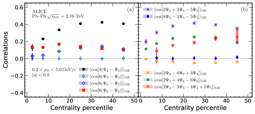
Figure 1: Comparison of the extracted correlations between different combinations of two symmetry planes (a) and between three and four planes (b) using the GE in Eq. (4). Statistical (systematic) uncertainties are shown as lines (boxes).

The centrality dependence of the correlations between different combinations of two and three symmetry planes, as well as the first measurement of a correlation between four planes, are presented in Fig. 1. In the case of two symmetry planes shown in Fig. 1(a), the strongest correlation is observed for $\langle\cos\left[4\left(\Psi_{4}-\Psi_{2}\right)\right]\rangle_{\text{GE}}$, while the correlation strength gets weaker for $\langle\cos\left[6\left(\Psi_{6}-\Psi_{2}\right)\right]\rangle_{\text{GE}}$ and $\langle\cos\left[6\left(\Psi_{6}-\Psi_{3}\right)\right]\rangle_{\text{GE}}$. The results for $\langle\cos\left[6\left(\Psi_{2}-\Psi_{3}\right)\right]\rangle_{\text{GE}}$ are compatible with zero within uncertainties. A hierarchy, $\langle\cos\left[4\left(\Psi_{4}-\Psi_{2}\right)\right]\rangle_{\text{GE}}$ $>$ $\langle\cos\left[6\left(\Psi_{6}-\Psi_{3}\right)\right]\rangle_{\text{GE}}$ $>$ $\langle\cos\left[6\left(\Psi_{6}-\Psi_{2}\right)\right]\rangle_{\text{GE}}$, holds for the centrality range 5–50%, with an exception of $\langle\cos\left[6\left(\Psi_{6}-\Psi_{3}\right)\right]\rangle_{\text{GE}}$ and $\langle\cos\left[6\left(\Psi_{6}-\Psi_{2}\right)\right]\rangle_{\text{GE}}$ being comparable at centralities above 20%. The details of the centrality dependence vary for the different combinations of symmetry planes. While $\langle\cos\left[4\left(\Psi_{4}-\Psi_{2}\right)\right]\rangle_{\text{GE}}$ and $\langle\cos\left[6\left(\Psi_{6}-\Psi_{2}\right)\right]\rangle_{\text{GE}}$ are increasing non-linearly from central to semicentral collisions, $\langle\cos\left[6\left(\Psi_{6}-\Psi_{3}\right)\right]\rangle_{\text{GE}}$ shows a weak centrality dependence. The observed zero signal for $\langle\cos\left[6\left(\Psi_{2}-\Psi_{3}\right)\right]\rangle_{\text{GE}}$ indicates that no correlation is present within the current uncertainties for the final-state planes $\Psi_{2}$ and $\Psi_{3}$, while $v_{2}$ and $v_{3}$ are anti-correlated [58, 59, 73, 74, 26, 75, 44]. This result justifies the necessity of measuring separately correlations of symmetry planes and flow magnitudes, because these measurements can be used to independently constrain properties of the matter produced in heavy-ion collisions.

The different magnitudes of correlations are also observed for three symmetry planes as shown in Fig. 1(b). The magnitude and details of the centrality dependence vary for different combinations of flow harmonics. The $\langle\cos\left[2\Psi_{2}+3\Psi_{3}-5\Psi_{5}\right]\rangle_{\text{GE}}$ observable exhibits the strongest correlations and $\langle\cos\left[2\Psi_{2}-6\Psi_{3}+4\Psi_{4}\right]\rangle_{\text{GE}}$ shows the weaker signal. The SPC $\langle\cos\left[2\Psi_{2}-6\Psi_{3}+4\Psi_{4}\right]\rangle_{\text{GE}}$ is the only correlator with a negative sign, which will be discussed later on in more detail. The $\langle\cos\left[8\Psi_{2}-3\Psi_{3}-5\Psi_{5}\right]\rangle_{\text{GE}}$ observable is consistent with zero within uncertainties, similar to $\langle\cos\left[6\left(\Psi_{2}-\Psi_{3}\right)\right]\rangle_{\text{GE}}$. The correlation between four planes, $\langle\cos\left[2\Psi_{2}-3\Psi_{3}-4\Psi_{4}+5\Psi_{5}\right]\rangle_{\text{GE}}$ shows the strongest centrality dependence among all harmonic combinations and increases towards peripheral collisions.

The magnitudes of SPC are ordered approximately based on the corresponding order of the particle correlations. The two largest SPCs, $\langle\cos\left[4\left(\Psi_{4}-\Psi_{2}\right)\right]\rangle_{\text{GE}}$ and $\langle\cos\left[2\Psi_{2}+3\Psi_{3}-5\Psi_{5}\right]\rangle_{\text{GE}}$, are both measured with three-particle correlators. In contrast, the smallest ones are $\langle\cos\left[6\left(\Psi_{2}-\Psi_{3}\right)\right]\rangle_{\text{GE}}$ and $\langle\cos\left[8\Psi_{2}-3\Psi_{3}-5\Psi_{5}\right]\rangle_{\text{GE}}$, which are five- and six-particles correlations, respectively. One possible explanation is the following: the flow vector fluctuations encoded in the observed correlations are mainly attributed to the fluctuation of the initial state. Also, the initial state fluctuation is attributed to the fluctuation of a finite amount of “sources” produced at the degrees of freedom collision points, namely protons and neutrons, in the collision region. The Central Limit Theorem (CLT) states that for independent random variables (here, the position of sources), the sample average tends toward a Gaussian distribution when the number of sampling increases. A clear example of such behavior was studied for initial ellipticity in Ref. [76], where it was shown how the ellipticity fluctuation distribution changes from elliptic-power distribution with large skewness to a Gaussian distribution at a large number of sources. The order of particle correlations corresponds to the order of the cumulants of the underlying flow vector fluctuation. To see the clear connection, correlations should be written in a Cartesian notation rather than polar notation (see Refs. [77, 78, 79] for the relation between skewness and Kurtosis of flow vector distribution to the particle correlations). Only the second-order cumulant, namely the width of the distribution, is nonvanishing for a Gaussian distribution. As a result, higher-order cumulants (skewness, kurtosis, etc.) are small for distributions close to Gaussian. These studies are done for flow amplitudes with only one harmonic, but the logic is true for more than one harmonic as well. The observed ordering of magnitudes in Fig. 1 indicates that the contribution of higher-order cumulants is smaller compared to lower ones in general, meaning the lowest-order cumulants have the dominant role in deviation from Gaussianity. A crossing between $\langle\cos\left[6\left(\Psi_{6}-\Psi_{3}\right)\right]\rangle_{\text{GE}}$ (a three-particle correlation) and $\langle\cos\left[6\left(\Psi_{6}-\Psi_{2}\right)\right]\rangle_{\text{GE}}$ (a four-particle correlation) is observed with centralities above 25% where the number of final state particles is lower. The same is true for $\langle\cos\left[2\Psi_{2}+4\Psi_{4}-6\Psi_{6}\right]\rangle_{\text{GE}}$ (a three-particle correlation) and $\langle\cos\left[2\Psi_{2}-3\Psi_{3}-4\Psi_{4}+5\Psi_{5}\right]\rangle_{\text{GE}}$ (a four-particle correlation). The effect of non-Gaussianity is expected to be more dominant in this centrality region since the system size is smaller and less number of sources are expected. At a finite number of sources, the actual ordering of the correlation magnitudes depends on the details of the underlying source fluctuation that needs a separate study.

In Figs. 2 and 3 the experimental data for SPC estimated with the GE are compared with the results obtained from ATLAS [24] and ALICE [27] using the SP method. While the analysis of the SP method by ALICE used the same kinematic range as the work presented in this article, the analysis by ATLAS was performed in a wider range of $0.5~{}\text{GeV}/c<p_{\text{T}}$ and $|\eta|<2.5$. Despite this difference in kinematic regions, the SPC extracted by the SP method from ALICE and ATLAS agree within uncertainties. In general, the obtained data from the GE are significantly smaller than the estimates performed with the SP method for centralities larger than 10%. This difference is mainly attributed to the fact that correlations between flow amplitudes were not removed in the SP method as it was demonstrated in Ref. [15]. For the SPC $\langle\cos\left[4\left(\Psi_{4}-\Psi_{2}\right)\right]\rangle$ and $\langle\cos\left[6\left(\Psi_{6}-\Psi_{2}\right)\right]\rangle$ shown in Fig. 2, the GE and SP method are compatible only in 0–5% centrality, while for $\langle\cos\left[6\left(\Psi_{6}-\Psi_{3}\right)\right]\rangle$ the GE differs in all centrality intervals when compared to the SP method by ATLAS. For centralities larger than 5%, a clear splitting between all of the previously mentioned SPC is visible with significantly smaller values obtained by the GE. For $\langle\cos\left[6\left(\Psi_{2}-\Psi_{3}\right)\right]\rangle$ the experimental data of the GE are compatible with zero within the uncertainties in all considered centrality intervals. In contrast to that, the results of the SP method show a small, but non-zero value. However, the results obtained with the GE show larger uncertainties when compared to the SP for this particular SPC. Future studies with larger data sets will show whether the SPC $\langle\cos\left[6\left(\Psi_{2}-\Psi_{3}\right)\right]\rangle$ remains compatible with zero within uncertainties when using the GE or if a small non-zero correlation exists which cannot be resolved within the present uncertainties. In the latter case, the results of the GE will nonetheless lead to significantly smaller values than reported by the SP method.

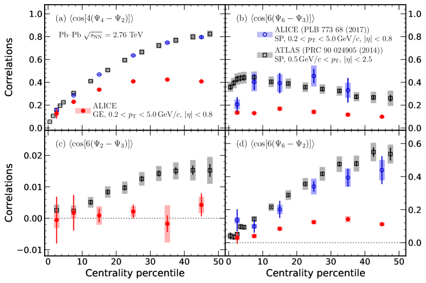
Figure 2: Experimental data of correlations between two symmetry planes obtained with the GE compared with measurements from ATLAS [24] and ALICE [27] using the SP method. Statistical and systematic uncertainties are represented by lines and boxes, respectively.

Similarly, the experimental results of the GE and the SP method are compared to each other for SPC between three planes. The results are presented in Fig. 3. For the combinations $\langle\cos\left[2\Psi_{2}+3\Psi_{3}-5\Psi_{5}\right]\rangle$, $\langle\cos\left[2\Psi_{2}+4\Psi_{4}-6\Psi_{6}\right]\rangle$ and $\langle\cos\left[2\Psi_{2}-6\Psi_{3}+4\Psi_{4}\right]\rangle$ the GE again leads to significantly smaller values than the SP method for centralities larger than 10%. For $\langle\cos\left[2\Psi_{2}+3\Psi_{3}-5\Psi_{5}\right]\rangle$ it has to be noted that the observables previously employed by ALICE [27] and ATLAS [24] differ in the denominator. ATLAS uses a fully factorized denominator $\langle v_{2}^{2}\rangle\langle v_{3}^{2}\rangle\langle v_{5}^{2}\rangle$ as in the definition of the SP method (5), while the denominator in the ALICE measurement is only partially factorized $\langle v_{2}^{2}v_{3}^{2}\rangle\langle v_{5}^{2}\rangle$ and thus is not defined exactly as in Eq. (5). To ease the notation in Fig. 3 we still label $\langle\cos\left[2\Psi_{2}+3\Psi_{3}-5\Psi_{5}\right]\rangle$ measured by ALICE [27] as SP method. The SPC $\langle\cos\left[8\Psi_{2}-3\Psi_{3}-5\Psi_{5}\right]\rangle$ is the only combination where the estimates by the GE and the SP method are compatible with each other within uncertainties in all considered centralities, as the results from the SP method are already close to zero. The difference in physical interpretation between the two SPC involving $\Psi_{2}$, $\Psi_{3}$ and $\Psi_{5}$ is discussed later.

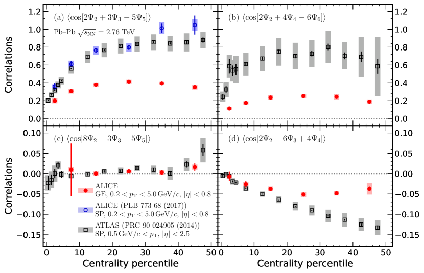
Figure 3: Correlations between three symmetry planes obtained with the GE compared with measurements from ATLAS [24] and ALICE [27] using the SP method. Statistical and systematic uncertainties are shown as lines and boxes, respectively.

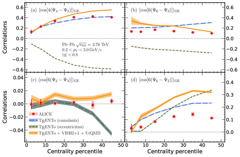
Figure 4: Experimental data for correlations between two symmetry planes compared to theoretical predictions in the initial and final state obtained with T${}_{\text{R}}$ENTo and T${}_{\text{R}}$ENTo+VISH(2+1)+UrQMD [80, 81, 82, 83, 84], respectively. For $\langle\cos\left[6\left(\Psi_{2}-\Psi_{3}\right)\right]\rangle_{\text{GE}}$ (c), the initial state predictions calculated via eccentricities and energy density cumulants, $\langle\cos[6(\phi_{2}-\phi_{3})]\rangle_{\text{GE}}$ and $\langle\cos[6(\Phi_{2}-\Phi_{3})]\rangle_{\text{GE}}$, fully overlap. Statistical (systematic) uncertainties of the ALICE data are shown as lines (boxes). The statistical uncertainties of the models are represented by the colored bands.

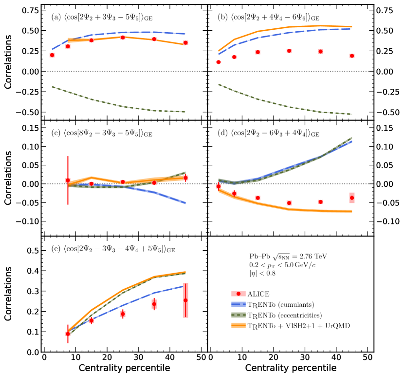
Figure 5: Experimental data for correlations between three (a-d) and four (e) symmetry planes compared with theoretical predictions in the initial and final state obtained with T${}_{\text{R}}$ENTo and T${}_{\text{R}}$ENTo+VISH(2+1)+UrQMD [80, 81, 82, 83, 84], respectively. Statistical (systematic) uncertainties of the ALICE data are shown as lines (boxes). The statistical uncertainties of the models are represented by the colored bands.

The new measurements of SPC with the GE are compared with Monte Carlo simulations with the T${}_{\text{R}}$ENTo+VISH(2+1)+UrQMD event generator [80, 81, 82, 83, 84]. In this article, the maximum a posteriori (MAP) estimation obtained in the Bayesian analysis in Ref. [7] is used for the parameters of the model. In inferring the MAP parameterization, a series of ALICE measurements (two- and four-particle correlations, charged particle multiplicities, etc.) were used as inputs into the Bayesian analysis, while the SPC are not included in these studies. Including new observables (e.g. SPC) in the Bayesian analysis can lead to an improvement in the uncertainty of the inferred parameter and resolving the discrepancies [12, 13]. If the discrepancy between model and data persists even after including new observables as input, the model itself needs to be revised.

In addition to the model predictions of final-state SPC, initial-state participant plane correlations are studied with T${}_{\text{R}}$ENTo. The participant plane of order $n$ takes the same role in the initial state as the symmetry plane in the final state. The correlations between participant planes are extracted from the initial state where flow vectors $v_{n}e^{in\Psi_{n}}$ are replaced first by eccentricities [85], and second by cumulants of the initial energy density [38, 86, 87]. The eccentricities are defined as

$$\epsilon_{n}e^{in\phi_{n}}=-\frac{\{r^{n}e^{in\varphi}\}}{\{r^{n}\}},\qquad n>1\,,$$ (6)

where $\{\cdots\}=\int r\text{d}r\text{d}\varphi\,\varepsilon(r,\varphi)$ stands for the average with respect to the initial energy density $\varepsilon(r,\varphi)$ in the transverse direction and $(r,\varphi)$ are the polar coordinates in the transverse plane. Eccentricities are the moments of the initial energy density distribution. The cumulants of the initial energy density distribution, $c_{n}e^{in\Phi_{n}}$, are obtained as a combination of eccentricities and the radial moments of the energy density, $\{r^{n}\}$. In fact, cumulants are a better measure to study the deformation of a distribution close to a Gaussian. Borrowing a motivating example from Ref. [86], a Gaussian distribution $e^{-x^{2}/2\sigma_{x}^{2}-y^{2}/2\sigma_{y}^{2}}$ has infinitely many non-vanishing moments, while only its second order cumulants are non-zero. Following the convention of Ref. [86], the first two cumulants and eccentricities are equivalent, $c_{n}e^{in\Phi_{n}}=\epsilon_{n}e^{in\phi_{n}}$ for $n=2,3$. Higher order cumulants have non-trivial relations to eccentricities. Here, only the fourth harmonic is shown as an example:

$$c_{4}e^{i4\Phi_{4}}=\epsilon_{4}e^{i4\phi_{4}}+3\left(\frac{\{r^{2}\}^{2}}{\{r^{4}\}}\right)\epsilon_{2}^{2}e^{i4\phi_{2}}.$$ (7)

More details can be found in Refs. [38, 86, 87].

The comparison with initial and final state SPC demonstrates how much of the observed correlation is inherited from the initial state. This is due to the linear and non-linear response of the medium [88]. For the second- and third-order anisotropies, the linear response is expected to dominate i.e. $v_{2}e^{i2\Psi_{2}}=\omega_{2}c_{2}e^{i2\Phi_{2}}$ and $v_{3}e^{i3\Psi_{3}}=\omega_{3}c_{3}e^{i3\Phi_{3}}$, especially in central and semicentral collisions [85, 73, 89]. The $\omega_{i}$ describe the linear hydrodynamic coupling constants. For higher orders, non-linear contributions will play a significant role, e.g. in case of the fourth order as

$$v_{4}e^{i4\Psi_{4}}=\omega_{4}c_{4}e^{i4\Phi_{4}}+\omega_{422}c_{2}^{2}e^{i4\Phi_{2}}\,,$$ (8)

where $\omega_{422}$ is the non-linear coupling between the second- and fourth-order anisotropies [38, 86, 87]. As an example of how this impacts the SPC, one can build the quantity $v_{2}^{2}v_{4}e^{i4(\Psi_{4}-\Psi_{2})}$. The real part of its phase corresponds to the SPC $\langle\cos\left[4\left(\Psi_{4}-\Psi_{2}\right)\right]\rangle$. Using the linear and non-linear response, one can translate this into the initial state as:

$$v_{2}^{2}v_{4}e^{i4(\Psi_{4}-\Psi_{2})}=\omega_{2}\omega_{4}c_{2}^{2}c_{4}e^{i4\left(\Phi_{4}-\Phi_{2}\right)}+\omega_{422}\omega_{2}^{2}c_{2}^{2}\,.$$ (9)

The latter equation shows that the initial and final state SPC $\langle\cos\left[4\left(\Psi_{4}-\Psi_{2}\right)\right]\rangle$ will be equal to each other in the limit of pure linear response, while they will deviate in case of a non-zero non-linear coupling $\omega_{422}$.

Figure 4 shows the comparison between the model calculations and the experimental data for the correlation between two symmetry planes. For the SPC $\langle\cos\left[4\left(\Psi_{4}-\Psi_{2}\right)\right]\rangle_{\text{GE}}$ the initial-state participant plane correlations given by the energy density cumulants overlap with the final-state prediction of the SPC up to 10% in centrality, indicating a vanishing non-linear coupling in the regime dominated by flow fluctuations. For higher centralities, the two curves increasingly deviate, showing the presence of a non-zero non-linear coupling between the second- and fourth-order flow vectors. In particular, it can be observed that the final-state prediction increasingly deviates from the data with increasing centrality. This is expected, since in this regime strong correlations between the second and fourth harmonics can originate from the initial ellipsoidal geometry. The non-linear coupling constant between initial-state ellipticity and $v_{4}e^{i4\Psi_{4}}$ from T${}_{\text{R}}$ENTo to iEBE-VISHNU was studied in Ref. [90]. It was demonstrated that this coupling is very small up to 10% and it is positive up to 70% centrality. For $\langle\cos\left[6\left(\Psi_{2}-\Psi_{3}\right)\right]\rangle_{\text{GE}}$ the experimental data show a flat centrality behavior and are compatible with zero within the uncertainties. The model predicts small values for $\langle\cos\left[6\left(\Psi_{2}-\Psi_{3}\right)\right]\rangle_{\text{GE}}$ with a flat centrality behavior although the predictions for the final state slightly overestimate the data. However, the initial-state correlations decrease to more negative values for centralities above 30%. For $\langle\cos\left[6\left(\Psi_{2}-\Psi_{3}\right)\right]\rangle_{\text{GE}}$, a linear response is expected to be an accurate approximation for harmonics $n=2,3$ in central and semicentral collisions [85, 73, 89]. As such, one would expect that the initial state participant plane correlations should be the same as the final state symmetry plane correlations between the second- and third-order harmonics. One possible explanation is that higher-order terms beyond linear response are responsible for decreasing the correlation during the hydrodynamic evolution, and the final value accidentally lands on very small numbers. In this respect, more rigorous study is needed in the future. While the model captures the qualitative behavior of the experimental signal in the two previous cases, a quantitative agreement is not observed in every case, particularly not for SPC involving $\Psi_{6}$ or correlations between four symmetry planes. For the SPC $\langle\cos\left[6\left(\Psi_{6}-\Psi_{2}\right)\right]\rangle_{\text{GE}}$ and $\langle\cos\left[6\left(\Psi_{6}-\Psi_{3}\right)\right]\rangle_{\text{GE}}$, a large deviation between the data and the final-state model prediction can be observed. This deviation could be related to the complex dynamics of the sixth-order symmetry plane, which involves multiple non-linear responses to the lower order symmetry planes $\Psi_{2}$, $\Psi_{3}$ and $\Psi_{4}$. For the SPC $\langle\cos\left[6\left(\Psi_{6}-\Psi_{3}\right)\right]\rangle_{\text{GE}}$ it is in particular interesting that the initial-state correlation becomes stronger with increasing centrality, while the final-state correlation becomes weaker with increasing centrality in the model. In contrast to that, the experimental data shows only a very weak centrality dependence.

The sign change between correlations obtained from eccentricities (green short-dashed curves) and initial energy density cumulants (blue long-dashed curves) in Fig. 4 was pointed out in Ref. [87]. The actual shape of the initial state is captured by $c_{n}e^{in\Phi_{n}}$. As a result, the linear hydrodynamic response approximation is more accurate when employing cumulants. As an example, SPC $\langle\cos\left[4\left(\Psi_{4}-\Psi_{2}\right)\right]\rangle_{\text{GE}}$ in Fig. 4 panel (a) is considered. Referring to Eq. (7), the difference between $\epsilon_{4}e^{in\phi_{4}}$ and $c_{4}e^{in\Phi_{4}}$ is proportional to $\{r^{2}\}^{2}/\{r^{4}\}$, which merely depends on the radial shape of the initial state. The numerator of the correlation $\langle\cos(4\phi_{2}-4\phi_{4})\rangle_{\text{GE}}$ is proportional to the real part of $\langle\epsilon_{2}^{2}\epsilon_{4}e^{4i\phi_{2}-4i\phi_{4}}\rangle$. Substituting from Eq. (7) ($c_{2}e^{2i\Phi_{2}}$ and $\epsilon_{2}e^{2i\phi_{2}}$ are identical), one finds $\langle\epsilon_{2}^{2}\epsilon_{4}e^{4i\phi_{2}-4i\phi_{4}}\rangle=\langle c_{2}^{2}c_{4}e^{4i\Phi_{2}-4i\Phi_{4}}\rangle-3\langle(\{r^{2}\}^{2}/\{r^{4}\})c_{2}^{4}\rangle$. In case the second term on the right is small, SPC of cumulants are expected to be close to those calculated from eccentricities. However, noting that $3\langle(\{r^{2}\}^{2}/\{r^{4}\})c_{2}^{4}\rangle$ is real and positive, the contribution of this term is such that it leads to a negative sign for $\langle\epsilon_{2}^{2}\epsilon_{4}e^{4i\phi_{2}-4i\phi_{4}}\rangle$. Therefore, one concludes that, regarding the hydrodynamic response, using energy-density cumulants for the initial state is more appropriate. A more detailed study can be found in Ref. [90].

In Fig. 5, the same comparison of model predictions with respect to the experimental data was performed for SPC involving three or four symmetry planes. For the SPC $\langle\cos\left[2\Psi_{2}+3\Psi_{3}-5\Psi_{5}\right]\rangle_{\text{GE}}$, a non-zero correlation signal was extracted, which existed to a larger extent already in the initial state. The final-state predictions of T${}_{\text{R}}$ENTo+iEBE-VISHNU are in good agreement with the experimental data. Further considering the same three symmetry planes $\Psi_{2}$, $\Psi_{3}$ and $\Psi_{5}$, the combination $\langle\cos\left[8\Psi_{2}-3\Psi_{3}-5\Psi_{5}\right]\rangle_{\text{GE}}$ results in an experimental signal that is compatible with zero within uncertainties for all reported centrality intervals. The deviation between $\langle\cos\left[2\Psi_{2}+3\Psi_{3}-5\Psi_{5}\right]\rangle_{\text{GE}}$ and $\langle\cos\left[8\Psi_{2}-3\Psi_{3}-5\Psi_{5}\right]\rangle_{\text{GE}}$ can be attributed to different contributions from the initial-state in the non-linear response of the two observables. While the non-linear response term for $\langle\cos\left[2\Psi_{2}+3\Psi_{3}-5\Psi_{5}\right]\rangle_{\text{GE}}$ does not contain contributions from any participant plane correlations, the non-linear part of $\langle\cos\left[8\Psi_{2}-3\Psi_{3}-5\Psi_{5}\right]\rangle_{\text{GE}}$ picks up such an additional correlation from the initial state. In particular, the SPC $\langle\cos\left[8\Psi_{2}-3\Psi_{3}-5\Psi_{5}\right]\rangle_{\text{GE}}$ has a non-linear coupling to the initial-state correlation between the second- and third-order participant planes. Similar to previously presented examples of SPC that involve the sixth-order symmetry plane $\Psi_{6}$, the final-state model prediction for $\langle\cos\left[2\Psi_{2}+4\Psi_{4}-6\Psi_{6}\right]\rangle_{\text{GE}}$ shows a large deviation compared to the measurements. This deviation is again attributed to the complexity of $\Psi_{6}$, which makes it particularly sensitive to the model parameters. One finds that $\langle\cos\left[2\Psi_{2}+3\Psi_{3}-5\Psi_{5}\right]\rangle_{\text{GE}}$ has the strongest signal in data while $\langle\cos\left[2\Psi_{2}+4\Psi_{4}-6\Psi_{6}\right]\rangle_{\text{GE}}$ is larger than $\langle\cos\left[2\Psi_{2}+3\Psi_{3}-5\Psi_{5}\right]\rangle_{\text{GE}}$ in the model. The results of $\langle\cos\left[2\Psi_{2}-6\Psi_{3}+4\Psi_{4}\right]\rangle_{\text{GE}}$ are the only measurement with a negative signal for the SPC. While the model predicts this behavior as well, it can be observed that the initial-state correlations are strictly non-negative. Thus, the sign-change between the initial and final state can be linked to the hydrodynamic evolution of the system. Lastly, Fig. 5 shows the comparison with the first experimental measurement of correlations between four symmetry planes. While the final-state model prediction captures the qualitative behavior, a quantitative agreement between experimental data and model is not observed. A recent Bayesian analysis of the QGP hydrodynamic properties [13] has shown that higher-order correlations as well as measurements involving higher order flow harmonics are more sensitive to changes in the QGP parameters. Thus, in particular the measurements of SPC including $\Psi_{6}$ and the correlations between four symmetry planes are expected to give more stringent constraints in future analyses of this kind.

4 Conclusion

Utilizing the recently introduced Gaussian Estimator, the first measurements of symmetry plane correlations, which are not influenced by correlations between different flow amplitudes, are presented in Pb–Pb collisions at $\sqrt{s_{\text{NN}}}=$ 2.76 TeV. Correlations between two, three and, for the first time, four symmetry planes were shown. The data show a clear order for the different SPC, which can be related to the cumulants of the underlying flow vector fluctuations. The measurements using the new GE show significantly smaller symmetry plane correlations than previously reported by the SP method. This observation is in qualitative agreement with the study in Ref. [15] which reported the bias of the SP method to larger values due to the influence of correlations between the flow amplitudes. In contrast to the SP method, the results of $\langle\cos\left[6\left(\Psi_{2}-\Psi_{3}\right)\right]\rangle_{\text{GE}}$ are consistent with zero with the current uncertainties. Within the uncertainties, this shows that $\Psi_{2}$ and $\Psi_{3}$ are fully uncorrelated, which was qualitatively reported by a previous ALICE study [23]. Future studies using Run 2 Pb–Pb data as well as the upcoming Run 3 Pb–Pb campaign will show whether a small non-zero correlation exists between $\Psi_{2}$ and $\Psi_{3}$, which cannot be resolved within the present uncertainties. Employing state-of-the-art hydrodynamic model calculations, one could see that the predictions and the measurements are not in quantitative agreement for all SPC. The most significant deviations are observed in the correlations $\langle\cos\left[6\left(\Psi_{6}-\Psi_{3}\right)\right]\rangle_{\text{GE}}$, $\langle\cos\left[6\left(\Psi_{6}-\Psi_{2}\right)\right]\rangle_{\text{GE}}$, $\langle\cos\left[2\Psi_{2}+4\Psi_{4}-6\Psi_{6}\right]\rangle_{\text{GE}}$ and $\langle\cos\left[2\Psi_{2}-3\Psi_{3}-4\Psi_{4}+5\Psi_{5}\right]\rangle_{\text{GE}}$. Future studies have to address how the initial state correlations between the second- and third-order participant planes are suppressed in the final state SPC $\langle\cos\left[6\left(\Psi_{2}-\Psi_{3}\right)\right]\rangle_{\text{GE}}$ as one would expect linear response to be a good approximation for the second- and third-order flow harmonics. Since the measured SPC contain independent information about flow vector fluctuations, they will provide useful inputs for future Bayesian analyses aiming at extracting the properties of the QGP.

Appendix A A brief overview of the Gaussian Estimator

The details of the derivation and validation of the GE in Eq. (4) can be found in Ref. [15]. In the following, a brief overview of the main idea is presented. The concept of the GE is similar to estimating the average elliptic flow originating from the geometry of the collision by using the flow measurements $v_{2}\{2k\}$. To briefly explain, let us define $v_{2,x}=v_{2}\cos 2(\Psi_{2}-\Psi_{\text{RP}})$ and $v_{2,y}=v_{2}\sin 2(\Psi_{2}-\Psi_{\text{RP}})$. Since $\Psi_{2}$ fluctuates around the reaction plane angle $\Psi_{\text{RP}}$, the average $\overline{v}_{2}=\langle v_{2,x}\rangle$ depends merely on the nonzero average of the initial elliptic shape and $\langle v_{2,y}\rangle$ vanishes [92]. However, the angle $\Psi_{\text{RP}}$ rotates randomly event-by-event in the experiment, therefore, $\overline{v}_{2}$ is not accessible directly. To estimate the value of $\overline{v}_{2}$, one employs the central limit theorem to approximate the fluctuation of $(v_{2,x},v_{2,y})$ as a 2D Gaussian proportional to $\exp\left[-((v_{2,x}-\overline{v}_{2})^{2}+v_{2,y}^{2})/2\sigma_{v}^{2}\right]=\exp\left[-(v_{2}^{2}+\overline{v}_{2}^{2}-2v_{2}\overline{v}_{2}\cos 2\Psi_{2})/2\sigma_{v}^{2}\right]$. By averaging over $\Psi_{2}$, one finds a Bessel–Gaussian distribution depending on the random variable $v_{2}$ where $\overline{v}_{2}$ is a parameter that controls the shape of the distribution [14, 93, 92]. Using this information, one finds the estimation $\overline{v}_{2}\approx v_{2}\{2k\}$ for $k>1$ [92].

To explain the idea behind Eq. (4), the SPC $\langle\cos 4(\Psi_{4}-\Psi_{2})\rangle$ is considered as a simple. More general cases can be obtained accordingly. In order to estimate $\langle\cos 4(\Psi_{4}-\Psi_{2})\rangle$ in terms of quantities such as $\langle v_{2}^{2}v_{4}\cos 4(\Psi_{4}-\Psi_{2})\rangle$, the two variables $R=v_{2}^{2}v_{4}$ and $\theta=4(\Psi_{4}-\Psi_{2})$ are defined, or in Cartesian form $R_{x}=R\cos\theta$ and $R_{y}=R\sin\theta$. Since $R$ and $\theta$ are correlated, the ratio $\langle R\cos\theta\rangle/\langle R\rangle$ would not be equal to $\langle\cos\theta\rangle$. However, the $(R_{x},R_{y})$ fluctuation can be approximated with a 2D Gaussian distribution,

$$N(R_{x},R_{y})=\frac{1}{\pi\sigma_{R}^{2}}\exp\left[-\frac{(R_{x}-\mu_{x})^{2}+R_{y}^{2}}{\sigma_{R}^{2}}\right],$$ (10)

where

$$\mu_{x}=\langle R_{x}\rangle=\langle v_{2}^{2}v_{4}\cos 4(\Psi_{4}-\Psi_{2})\rangle,\qquad\sigma_{R}\approx\sqrt{\langle R_{x}^{2}\rangle+\langle R_{y}^{2}\rangle}=\sqrt{\langle v_{2}^{4}v_{4}^{2}\rangle}.$$ (11)

The equation (10) in polar coordinates is proportional to $\exp[-(R^{2}+\mu_{x}^{2}-2R\mu_{x}\cos\theta)/\sigma_{R}^{2}]$. Averaging over the variable $\theta$ would lead to a Bessel-Gaussian distribution. However, the goal of this study is the extraction of information about $\cos\theta$ fluctuations. Therefore, one needs to average out the variable $R$ to find a distribution that depends on $\theta$ only. As a result, one finds

$$\langle\cos\theta\rangle\approx\sqrt{\frac{\pi}{4}}\left(\frac{\mu_{x}}{\sigma_{R}}\right),$$ (12)

where the prefactor $\sqrt{\pi/4}\approx 0.886$ is the consequence of integration over $R$ and $\theta$ in the calculation of $\langle\cos\theta\rangle$. Substituting Eq. (11) into Eq. (12), one finds

$$\langle\cos 4(\Psi_{4}-\Psi_{2})\rangle_{\text{GE}}=\sqrt{\frac{\pi}{4}}\;\frac{\langle v_{2}^{2}v_{4}\cos 4(\Psi_{4}-\Psi_{2})\rangle}{\sqrt{\langle v_{2}^{4}v_{4}^{2}\rangle}},$$ (13)

which is a special case of Eq. (4). To derive the analytical expression in Eq. (12), an expansion up to leading terms with respect to $\mu_{x}/\sigma_{R}$ was considered. Also it has been assumed that $\langle R_{x}^{2}\rangle\approx\langle R_{y}^{2}\rangle$. On top of these assumptions, the $(R_{x},R_{y})$ fluctuation should be close to a 2D Gaussian to have an accurate estimation. Comparing with the true values of the SPC in the hydrodynamic simulations, it turns out that these approximations lead to an accurate estimation [15]. In the scalar product method, the correlation is given by

$$\langle\cos 4(\Psi_{4}-\Psi_{2})\rangle_{\text{SP}}=\frac{\langle v_{2}^{2}v_{4}\cos 4(\Psi_{4}-\Psi_{2})\rangle}{\sqrt{\langle v_{2}^{4}\rangle\langle v_{4}^{2}\rangle}}.$$ (14)

Apart from the numerical prefactor, the denominator of GE contains a joint correlation $\langle v_{2}^{4}v_{4}^{2}\rangle$ rather than $\langle v_{2}^{4}\rangle\langle v_{4}^{2}\rangle$ as in the SP method.

Appendix B The ALICE Collaboration

S. Acharya  ¹²⁵, D. Adamová  ⁸⁶, A. Adler⁶⁹, G. Aglieri Rinella  ³², M. Agnello  ²⁹, N. Agrawal  ⁵⁰, Z. Ahammed  ¹³², S. Ahmad  ¹⁵, S.U. Ahn  ⁷⁰, I. Ahuja  ³⁷, A. Akindinov  ¹⁴⁰, M. Al-Turany  ⁹⁷, D. Aleksandrov  ¹⁴⁰, B. Alessandro  ⁵⁵, H.M. Alfanda  ⁶, R. Alfaro Molina  ⁶⁶, B. Ali  ¹⁵, A. Alici  ²⁵, N. Alizadehvandchali  ¹¹⁴, A. Alkin  ³², J. Alme  ²⁰, G. Alocco  ⁵¹, T. Alt  ⁶³, I. Altsybeev  ¹⁴⁰, M.N. Anaam  ⁶, C. Andrei  ⁴⁵, A. Andronic  ¹³⁵, V. Anguelov  ⁹⁴, F. Antinori  ⁵³, P. Antonioli  ⁵⁰, N. Apadula  ⁷⁴, L. Aphecetche  ¹⁰³, H. Appelshäuser  ⁶³, C. Arata  ⁷³, S. Arcelli  ²⁵, M. Aresti  ⁵¹, R. Arnaldi  ⁵⁵, J.G.M.C.A. Arneiro  ¹¹⁰, I.C. Arsene  ¹⁹, M. Arslandok  ¹³⁷, A. Augustinus  ³², R. Averbeck  ⁹⁷, M.D. Azmi  ¹⁵, A. Badalà  ⁵², J. Bae  ¹⁰⁴, Y.W. Baek  ⁴⁰, X. Bai  ¹¹⁸, R. Bailhache  ⁶³, Y. Bailung  ⁴⁷, A. Balbino  ²⁹, A. Baldisseri  ¹²⁸, B. Balis  ², D. Banerjee  ⁴, Z. Banoo  ⁹¹, R. Barbera  ²⁶, F. Barile  ³¹, L. Barioglio  ⁹⁵, M. Barlou⁷⁸, G.G. Barnaföldi  ¹³⁶, L.S. Barnby  ⁸⁵, V. Barret  ¹²⁵, L. Barreto  ¹¹⁰, C. Bartels  ¹¹⁷, K. Barth  ³², E. Bartsch  ⁶³, N. Bastid  ¹²⁵, S. Basu  ⁷⁵, G. Batigne  ¹⁰³, D. Battistini  ⁹⁵, B. Batyunya  ¹⁴¹, D. Bauri⁴⁶, J.L. Bazo Alba  ¹⁰¹, I.G. Bearden  ⁸³, C. Beattie  ¹³⁷, P. Becht  ⁹⁷, D. Behera  ⁴⁷, I. Belikov  ¹²⁷, A.D.C. Bell Hechavarria  ¹³⁵, F. Bellini  ²⁵, R. Bellwied  ¹¹⁴, S. Belokurova  ¹⁴⁰, V. Belyaev  ¹⁴⁰, G. Bencedi  ¹³⁶, S. Beole  ²⁴, A. Bercuci  ⁴⁵, Y. Berdnikov  ¹⁴⁰, A. Berdnikova  ⁹⁴, L. Bergmann  ⁹⁴, M.G. Besoiu  ⁶², L. Betev  ³², P.P. Bhaduri  ¹³², A. Bhasin  ⁹¹, M.A. Bhat  ⁴, B. Bhattacharjee  ⁴¹, L. Bianchi  ²⁴, N. Bianchi  ⁴⁸, J. Bielčík  ³⁵, J. Bielčíková  ⁸⁶, J. Biernat  ¹⁰⁷, A.P. Bigot  ¹²⁷, A. Bilandzic  ⁹⁵, G. Biro  ¹³⁶, S. Biswas  ⁴, N. Bize  ¹⁰³, J.T. Blair  ¹⁰⁸, D. Blau  ¹⁴⁰, M.B. Blidaru  ⁹⁷, N. Bluhme³⁸, C. Blume  ⁶³, G. Boca  ^21,54, F. Bock  ⁸⁷, T. Bodova  ²⁰, A. Bogdanov¹⁴⁰, S. Boi  ²², J. Bok  ⁵⁷, L. Boldizsár  ¹³⁶, M. Bombara  ³⁷, P.M. Bond  ³², G. Bonomi  ^131,54, H. Borel  ¹²⁸, A. Borissov  ¹⁴⁰, A.G. Borquez Carcamo  ⁹⁴, H. Bossi  ¹³⁷, E. Botta  ²⁴, Y.E.M. Bouziani  ⁶³, L. Bratrud  ⁶³, P. Braun-Munzinger  ⁹⁷, M. Bregant  ¹¹⁰, M. Broz  ³⁵, G.E. Bruno  ^96,31, M.D. Buckland  ²³, D. Budnikov  ¹⁴⁰, H. Buesching  ⁶³, S. Bufalino  ²⁹, P. Buhler  ¹⁰², Z. Buthelezi  ^67,121, A. Bylinkin  ²⁰, S.A. Bysiak¹⁰⁷, M. Cai  ⁶, H. Caines  ¹³⁷, A. Caliva  ⁹⁷, E. Calvo Villar  ¹⁰¹, J.M.M. Camacho  ¹⁰⁹, P. Camerini  ²³, F.D.M. Canedo  ¹¹⁰, M. Carabas  ¹²⁴, A.A. Carballo  ³², F. Carnesecchi  ³², R. Caron  ¹²⁶, L.A.D. Carvalho  ¹¹⁰, J. Castillo Castellanos  ¹²⁸, F. Catalano  ²⁴, C. Ceballos Sanchez  ¹⁴¹, I. Chakaberia  ⁷⁴, P. Chakraborty  ⁴⁶, S. Chandra  ¹³², S. Chapeland  ³², M. Chartier  ¹¹⁷, S. Chattopadhyay  ¹³², S. Chattopadhyay  ⁹⁹, T.G. Chavez  ⁴⁴, T. Cheng  ^97,6, C. Cheshkov  ¹²⁶, B. Cheynis  ¹²⁶, V. Chibante Barroso  ³², D.D. Chinellato  ¹¹¹, E.S. Chizzali  ^II,95, J. Cho  ⁵⁷, S. Cho  ⁵⁷, P. Chochula  ³², P. Christakoglou  ⁸⁴, C.H. Christensen  ⁸³, P. Christiansen  ⁷⁵, T. Chujo  ¹²³, M. Ciacco  ²⁹, C. Cicalo  ⁵¹, F. Cindolo  ⁵⁰, M.R. Ciupek⁹⁷, G. Clai^III,50, F. Colamaria  ⁴⁹, J.S. Colburn¹⁰⁰, D. Colella  ^96,31, M. Colocci  ²⁵, G. Conesa Balbastre  ⁷³, Z. Conesa del Valle  ⁷², G. Contin  ²³, J.G. Contreras  ³⁵, M.L. Coquet  ¹²⁸, T.M. Cormier^I,87, P. Cortese  ^130,55, M.R. Cosentino  ¹¹², F. Costa  ³², S. Costanza  ^21,54, C. Cot  ⁷², J. Crkovská  ⁹⁴, P. Crochet  ¹²⁵, R. Cruz-Torres  ⁷⁴, P. Cui  ⁶, A. Dainese  ⁵³, M.C. Danisch  ⁹⁴, A. Danu  ⁶², P. Das  ⁸⁰, P. Das  ⁴, S. Das  ⁴, A.R. Dash  ¹³⁵, S. Dash  ⁴⁶, A. De Caro  ²⁸, G. de Cataldo  ⁴⁹, J. de Cuveland³⁸, A. De Falco  ²², D. De Gruttola  ²⁸, N. De Marco  ⁵⁵, C. De Martin  ²³, S. De Pasquale  ²⁸, R. Deb¹³¹, S. Deb  ⁴⁷, R.J. Debski  ², K.R. Deja¹³³, R. Del Grande  ⁹⁵, L. Dello Stritto  ²⁸, W. Deng  ⁶, P. Dhankher  ¹⁸, D. Di Bari  ³¹, A. Di Mauro  ³², R.A. Diaz  ^141,7, T. Dietel  ¹¹³, Y. Ding  ⁶, R. Divià  ³², D.U. Dixit  ¹⁸, Ø. Djuvsland²⁰, U. Dmitrieva  ¹⁴⁰, A. Dobrin  ⁶², B. Dönigus  ⁶³, J.M. Dubinski¹³³, A. Dubla  ⁹⁷, S. Dudi  ⁹⁰, P. Dupieux  ¹²⁵, M. Durkac¹⁰⁶, N. Dzalaiova¹², T.M. Eder  ¹³⁵, R.J. Ehlers  ⁷⁴, V.N. Eikeland²⁰, F. Eisenhut  ⁶³, D. Elia  ⁴⁹, B. Erazmus  ¹⁰³, F. Ercolessi  ²⁵, F. Erhardt  ⁸⁹, M.R. Ersdal²⁰, B. Espagnon  ⁷², G. Eulisse  ³², D. Evans  ¹⁰⁰, S. Evdokimov  ¹⁴⁰, L. Fabbietti  ⁹⁵, M. Faggin  ²⁷, J. Faivre  ⁷³, F. Fan  ⁶, W. Fan  ⁷⁴, A. Fantoni  ⁴⁸, M. Fasel  ⁸⁷, P. Fecchio²⁹, A. Feliciello  ⁵⁵, G. Feofilov  ¹⁴⁰, A. Fernández Téllez  ⁴⁴, L. Ferrandi  ¹¹⁰, M.B. Ferrer  ³², A. Ferrero  ¹²⁸, C. Ferrero  ⁵⁵, A. Ferretti  ²⁴, V.J.G. Feuillard  ⁹⁴, V. Filova³⁵, D. Finogeev  ¹⁴⁰, F.M. Fionda  ⁵¹, F. Flor  ¹¹⁴, A.N. Flores  ¹⁰⁸, S. Foertsch  ⁶⁷, I. Fokin  ⁹⁴, S. Fokin  ¹⁴⁰, E. Fragiacomo  ⁵⁶, E. Frajna  ¹³⁶, U. Fuchs  ³², N. Funicello  ²⁸, C. Furget  ⁷³, A. Furs  ¹⁴⁰, T. Fusayasu  ⁹⁸, J.J. Gaardhøje  ⁸³, M. Gagliardi  ²⁴, A.M. Gago  ¹⁰¹, C.D. Galvan  ¹⁰⁹, D.R. Gangadharan  ¹¹⁴, P. Ganoti  ⁷⁸, C. Garabatos  ⁹⁷, J.R.A. Garcia  ⁴⁴, E. Garcia-Solis  ⁹, C. Gargiulo  ³², K. Garner¹³⁵, P. Gasik  ⁹⁷, A. Gautam  ¹¹⁶, M.B. Gay Ducati  ⁶⁵, M. Germain  ¹⁰³, A. Ghimouz¹²³, C. Ghosh¹³², M. Giacalone  ^50,25, P. Giubellino  ^97,55, P. Giubilato  ²⁷, A.M.C. Glaenzer  ¹²⁸, P. Glässel  ⁹⁴, E. Glimos¹²⁰, D.J.Q. Goh⁷⁶, V. Gonzalez  ¹³⁴, M. Gorgon  ², S. Gotovac³³, V. Grabski  ⁶⁶, L.K. Graczykowski  ¹³³, E. Grecka  ⁸⁶, A. Grelli  ⁵⁸, C. Grigoras  ³², V. Grigoriev  ¹⁴⁰, S. Grigoryan  ^141,1, F. Grosa  ³², J.F. Grosse-Oetringhaus  ³², R. Grosso  ⁹⁷, D. Grund  ³⁵, G.G. Guardiano  ¹¹¹, R. Guernane  ⁷³, M. Guilbaud  ¹⁰³, K. Gulbrandsen  ⁸³, T. Gundem  ⁶³, T. Gunji  ¹²², W. Guo  ⁶, A. Gupta  ⁹¹, R. Gupta  ⁹¹, R. Gupta  ⁴⁷, S.P. Guzman  ⁴⁴, K. Gwizdziel  ¹³³, L. Gyulai  ¹³⁶, M.K. Habib⁹⁷, C. Hadjidakis  ⁷², F.U. Haider  ⁹¹, H. Hamagaki  ⁷⁶, A. Hamdi  ⁷⁴, M. Hamid⁶, Y. Han  ¹³⁸, R. Hannigan  ¹⁰⁸, M.R. Haque  ¹³³, J.W. Harris  ¹³⁷, A. Harton  ⁹, H. Hassan  ⁸⁷, D. Hatzifotiadou  ⁵⁰, P. Hauer  ⁴², L.B. Havener  ¹³⁷, S.T. Heckel  ⁹⁵, E. Hellbär  ⁹⁷, H. Helstrup  ³⁴, M. Hemmer  ⁶³, T. Herman  ³⁵, G. Herrera Corral  ⁸, F. Herrmann¹³⁵, S. Herrmann  ¹²⁶, K.F. Hetland  ³⁴, B. Heybeck  ⁶³, H. Hillemanns  ³², B. Hippolyte  ¹²⁷, F.W. Hoffmann  ⁶⁹, B. Hofman  ⁵⁸, B. Hohlweger  ⁸⁴, G.H. Hong  ¹³⁸, M. Horst  ⁹⁵, A. Horzyk  ², Y. Hou  ⁶, P. Hristov  ³², C. Hughes  ¹²⁰, P. Huhn⁶³, L.M. Huhta  ¹¹⁵, C.V. Hulse  ⁷², T.J. Humanic  ⁸⁸, A. Hutson  ¹¹⁴, D. Hutter  ³⁸, J.P. Iddon  ¹¹⁷, R. Ilkaev¹⁴⁰, H. Ilyas  ¹³, M. Inaba  ¹²³, G.M. Innocenti  ³², M. Ippolitov  ¹⁴⁰, A. Isakov  ⁸⁶, T. Isidori  ¹¹⁶, M.S. Islam  ⁹⁹, M. Ivanov  ⁹⁷, M. Ivanov¹², V. Ivanov  ¹⁴⁰, M. Jablonski  ², B. Jacak  ⁷⁴, N. Jacazio  ³², P.M. Jacobs  ⁷⁴, S. Jadlovska¹⁰⁶, J. Jadlovsky¹⁰⁶, S. Jaelani  ⁸², L. Jaffe³⁸, C. Jahnke¹¹¹, M.J. Jakubowska  ¹³³, M.A. Janik  ¹³³, T. Janson⁶⁹, M. Jercic⁸⁹, S. Jia  ¹⁰, A.A.P. Jimenez  ⁶⁴, F. Jonas  ⁸⁷, J.M. Jowett   ^32,97, J. Jung  ⁶³, M. Jung  ⁶³, A. Junique  ³², A. Jusko  ¹⁰⁰, M.J. Kabus  ^32,133, J. Kaewjai¹⁰⁵, P. Kalinak  ⁵⁹, A.S. Kalteyer  ⁹⁷, A. Kalweit  ³², V. Kaplin  ¹⁴⁰, A. Karasu Uysal  ⁷¹, D. Karatovic  ⁸⁹, O. Karavichev  ¹⁴⁰, T. Karavicheva  ¹⁴⁰, P. Karczmarczyk  ¹³³, E. Karpechev  ¹⁴⁰, U. Kebschull  ⁶⁹, R. Keidel  ¹³⁹, D.L.D. Keijdener⁵⁸, M. Keil  ³², B. Ketzer  ⁴², S.S. Khade  ⁴⁷, A.M. Khan  ⁶, S. Khan  ¹⁵, A. Khanzadeev  ¹⁴⁰, Y. Kharlov  ¹⁴⁰, A. Khatun  ^116,15, A. Khuntia  ¹⁰⁷, M.B. Kidson¹¹³, B. Kileng  ³⁴, B. Kim  ¹⁰⁴, C. Kim  ¹⁶, D.J. Kim  ¹¹⁵, E.J. Kim  ⁶⁸, J. Kim  ¹³⁸, J.S. Kim  ⁴⁰, J. Kim  ⁶⁸, M. Kim  ^18,94, S. Kim  ¹⁷, T. Kim  ¹³⁸, K. Kimura  ⁹², S. Kirsch  ⁶³, I. Kisel  ³⁸, S. Kiselev  ¹⁴⁰, A. Kisiel  ¹³³, J.P. Kitowski  ², J.L. Klay  ⁵, J. Klein  ³², S. Klein  ⁷⁴, C. Klein-Bösing  ¹³⁵, M. Kleiner  ⁶³, T. Klemenz  ⁹⁵, A. Kluge  ³², A.G. Knospe  ¹¹⁴, C. Kobdaj  ¹⁰⁵, T. Kollegger⁹⁷, A. Kondratyev  ¹⁴¹, N. Kondratyeva  ¹⁴⁰, E. Kondratyuk  ¹⁴⁰, J. Konig  ⁶³, S.A. Konigstorfer  ⁹⁵, P.J. Konopka  ³², G. Kornakov  ¹³³, S.D. Koryciak  ², A. Kotliarov  ⁸⁶, V. Kovalenko  ¹⁴⁰, M. Kowalski  ¹⁰⁷, V. Kozhuharov  ³⁶, I. Králik  ⁵⁹, A. Kravčáková  ³⁷, L. Krcal  ^32,38, L. Kreis⁹⁷, M. Krivda  ^100,59, F. Krizek  ⁸⁶, K. Krizkova Gajdosova  ³², M. Kroesen  ⁹⁴, M. Krüger  ⁶³, D.M. Krupova  ³⁵, E. Kryshen  ¹⁴⁰, V. Kučera  ³², C. Kuhn  ¹²⁷, P.G. Kuijer  ⁸⁴, T. Kumaoka¹²³, D. Kumar¹³², L. Kumar  ⁹⁰, N. Kumar⁹⁰, S. Kumar  ³¹, S. Kundu  ³², P. Kurashvili  ⁷⁹, A. Kurepin  ¹⁴⁰, A.B. Kurepin  ¹⁴⁰, A. Kuryakin  ¹⁴⁰, S. Kushpil  ⁸⁶, J. Kvapil  ¹⁰⁰, M.J. Kweon  ⁵⁷, J.Y. Kwon  ⁵⁷, Y. Kwon  ¹³⁸, S.L. La Pointe  ³⁸, P. La Rocca  ²⁶, A. Lakrathok¹⁰⁵, M. Lamanna  ³², R. Langoy  ¹¹⁹, P. Larionov  ³², E. Laudi  ³², L. Lautner  ^32,95, R. Lavicka  ¹⁰², T. Lazareva  ¹⁴⁰, R. Lea  ^131,54, H. Lee  ¹⁰⁴, G. Legras  ¹³⁵, J. Lehrbach  ³⁸, T.M. Lelek², R.C. Lemmon  ⁸⁵, I. León Monzón  ¹⁰⁹, M.M. Lesch  ⁹⁵, E.D. Lesser  ¹⁸, P. Lévai  ¹³⁶, X. Li¹⁰, X.L. Li⁶, J. Lien  ¹¹⁹, R. Lietava  ¹⁰⁰, I. Likmeta  ¹¹⁴, B. Lim  ²⁴, S.H. Lim  ¹⁶, V. Lindenstruth  ³⁸, A. Lindner⁴⁵, C. Lippmann  ⁹⁷, A. Liu  ¹⁸, D.H. Liu  ⁶, J. Liu  ¹¹⁷, I.M. Lofnes  ²⁰, C. Loizides  ⁸⁷, S. Lokos  ¹⁰⁷, J. Lomker  ⁵⁸, P. Loncar  ³³, J.A. Lopez  ⁹⁴, X. Lopez  ¹²⁵, E. López Torres  ⁷, P. Lu  ^97,118, J.R. Luhder  ¹³⁵, M. Lunardon  ²⁷, G. Luparello  ⁵⁶, Y.G. Ma  ³⁹, A. Maevskaya¹⁴⁰, M. Mager  ³², A. Maire  ¹²⁷, M.V. Makariev  ³⁶, M. Malaev  ¹⁴⁰, G. Malfattore  ²⁵, N.M. Malik  ⁹¹, Q.W. Malik¹⁹, S.K. Malik  ⁹¹, L. Malinina  ^VI,141, D. Mal’Kevich  ¹⁴⁰, D. Mallick  ⁸⁰, N. Mallick  ⁴⁷, G. Mandaglio  ^30,52, S.K. Mandal  ⁷⁹, V. Manko  ¹⁴⁰, F. Manso  ¹²⁵, V. Manzari  ⁴⁹, Y. Mao  ⁶, G.V. Margagliotti  ²³, A. Margotti  ⁵⁰, A. Marín  ⁹⁷, C. Markert  ¹⁰⁸, P. Martinengo  ³², J.L. Martinez¹¹⁴, M.I. Martínez  ⁴⁴, G. Martínez García  ¹⁰³, S. Masciocchi  ⁹⁷, M. Masera  ²⁴, A. Masoni  ⁵¹, L. Massacrier  ⁷², A. Mastroserio  ^129,49, O. Matonoha  ⁷⁵, P.F.T. Matuoka¹¹⁰, A. Matyja  ¹⁰⁷, C. Mayer  ¹⁰⁷, A.L. Mazuecos  ³², F. Mazzaschi  ²⁴, M. Mazzilli  ³², J.E. Mdhluli  ¹²¹, A.F. Mechler⁶³, Y. Melikyan  ^43,140, A. Menchaca-Rocha  ⁶⁶, E. Meninno  ^102,28, A.S. Menon  ¹¹⁴, M. Meres  ¹², S. Mhlanga^113,67, Y. Miake¹²³, L. Micheletti  ⁵⁵, L.C. Migliorin¹²⁶, D.L. Mihaylov  ⁹⁵, K. Mikhaylov  ^141,140, A.N. Mishra  ¹³⁶, D. Miśkowiec  ⁹⁷, A. Modak  ⁴, A.P. Mohanty  ⁵⁸, B. Mohanty  ⁸⁰, M. Mohisin Khan  ^IV,15, M.A. Molander  ⁴³, Z. Moravcova  ⁸³, C. Mordasini  ⁹⁵, D.A. Moreira De Godoy  ¹³⁵, I. Morozov  ¹⁴⁰, A. Morsch  ³², T. Mrnjavac  ³², V. Muccifora  ⁴⁸, S. Muhuri  ¹³², J.D. Mulligan  ⁷⁴, A. Mulliri²², M.G. Munhoz  ¹¹⁰, R.H. Munzer  ⁶³, H. Murakami  ¹²², S. Murray  ¹¹³, L. Musa  ³², J. Musinsky  ⁵⁹, J.W. Myrcha  ¹³³, B. Naik  ¹²¹, A.I. Nambrath  ¹⁸, B.K. Nandi  ⁴⁶, R. Nania  ⁵⁰, E. Nappi  ⁴⁹, A.F. Nassirpour  ^17,75, A. Nath  ⁹⁴, C. Nattrass  ¹²⁰, M.N. Naydenov  ³⁶, A. Neagu¹⁹, A. Negru¹²⁴, L. Nellen  ⁶⁴, S.V. Nesbo³⁴, G. Neskovic  ³⁸, D. Nesterov  ¹⁴⁰, B.S. Nielsen  ⁸³, E.G. Nielsen  ⁸³, S. Nikolaev  ¹⁴⁰, S. Nikulin  ¹⁴⁰, V. Nikulin  ¹⁴⁰, F. Noferini  ⁵⁰, S. Noh  ¹¹, P. Nomokonov  ¹⁴¹, J. Norman  ¹¹⁷, N. Novitzky  ¹²³, P. Nowakowski  ¹³³, A. Nyanin  ¹⁴⁰, J. Nystrand  ²⁰, M. Ogino  ⁷⁶, A. Ohlson  ⁷⁵, V.A. Okorokov  ¹⁴⁰, J. Oleniacz  ¹³³, A.C. Oliveira Da Silva  ¹²⁰, M.H. Oliver  ¹³⁷, A. Onnerstad  ¹¹⁵, C. Oppedisano  ⁵⁵, A. Ortiz Velasquez  ⁶⁴, J. Otwinowski  ¹⁰⁷, M. Oya⁹², K. Oyama  ⁷⁶, Y. Pachmayer  ⁹⁴, S. Padhan  ⁴⁶, D. Pagano  ^131,54, G. Paić  ⁶⁴, A. Palasciano  ⁴⁹, S. Panebianco  ¹²⁸, H. Park  ¹²³, H. Park  ¹⁰⁴, J. Park  ⁵⁷, J.E. Parkkila  ³², R.N. Patra⁹¹, B. Paul  ²², H. Pei  ⁶, T. Peitzmann  ⁵⁸, X. Peng  ⁶, M. Pennisi  ²⁴, L.G. Pereira  ⁶⁵, D. Peresunko  ¹⁴⁰, G.M. Perez  ⁷, S. Perrin  ¹²⁸, Y. Pestov¹⁴⁰, V. Petráček  ³⁵, V. Petrov  ¹⁴⁰, M. Petrovici  ⁴⁵, R.P. Pezzi  ^103,65, S. Piano  ⁵⁶, M. Pikna  ¹², P. Pillot  ¹⁰³, O. Pinazza  ^50,32, L. Pinsky¹¹⁴, C. Pinto  ⁹⁵, S. Pisano  ⁴⁸, M. Płoskoń  ⁷⁴, M. Planinic⁸⁹, F. Pliquett⁶³, M.G. Poghosyan  ⁸⁷, B. Polichtchouk  ¹⁴⁰, S. Politano  ²⁹, N. Poljak  ⁸⁹, A. Pop  ⁴⁵, S. Porteboeuf-Houssais  ¹²⁵, V. Pozdniakov  ¹⁴¹, I.Y. Pozos  ⁴⁴, K.K. Pradhan  ⁴⁷, S.K. Prasad  ⁴, S. Prasad  ⁴⁷, R. Preghenella  ⁵⁰, F. Prino  ⁵⁵, C.A. Pruneau  ¹³⁴, I. Pshenichnov  ¹⁴⁰, M. Puccio  ³², S. Pucillo  ²⁴, Z. Pugelova¹⁰⁶, S. Qiu  ⁸⁴, L. Quaglia  ²⁴, R.E. Quishpe¹¹⁴, S. Ragoni  ¹⁴, A. Rakotozafindrabe  ¹²⁸, L. Ramello  ^130,55, F. Rami  ¹²⁷, S.A.R. Ramirez  ⁴⁴, T.A. Rancien⁷³, M. Rasa  ²⁶, S.S. Räsänen  ⁴³, R. Rath  ⁵⁰, M.P. Rauch  ²⁰, I. Ravasenga  ⁸⁴, K.F. Read  ^87,120, C. Reckziegel  ¹¹², A.R. Redelbach  ³⁸, K. Redlich  ^V,79, C.A. Reetz  ⁹⁷, A. Rehman²⁰, F. Reidt  ³², H.A. Reme-Ness  ³⁴, Z. Rescakova³⁷, K. Reygers  ⁹⁴, A. Riabov  ¹⁴⁰, V. Riabov  ¹⁴⁰, R. Ricci  ²⁸, M. Richter  ¹⁹, A.A. Riedel  ⁹⁵, W. Riegler  ³², C. Ristea  ⁶², M. Rodríguez Cahuantzi  ⁴⁴, K. Røed  ¹⁹, R. Rogalev  ¹⁴⁰, E. Rogochaya  ¹⁴¹, T.S. Rogoschinski  ⁶³, D. Rohr  ³², D. Röhrich  ²⁰, P.F. Rojas⁴⁴, S. Rojas Torres  ³⁵, P.S. Rokita  ¹³³, G. Romanenko  ¹⁴¹, F. Ronchetti  ⁴⁸, A. Rosano  ^30,52, E.D. Rosas⁶⁴, K. Roslon  ¹³³, A. Rossi  ⁵³, A. Roy  ⁴⁷, S. Roy  ⁴⁶, N. Rubini  ²⁵, O.V. Rueda  ¹¹⁴, D. Ruggiano  ¹³³, R. Rui  ²³, B. Rumyantsev¹⁴¹, P.G. Russek  ², R. Russo  ⁸⁴, A. Rustamov  ⁸¹, E. Ryabinkin  ¹⁴⁰, Y. Ryabov  ¹⁴⁰, A. Rybicki  ¹⁰⁷, H. Rytkonen  ¹¹⁵, W. Rzesa  ¹³³, O.A.M. Saarimaki  ⁴³, R. Sadek  ¹⁰³, S. Sadhu  ³¹, S. Sadovsky  ¹⁴⁰, J. Saetre  ²⁰, K. Šafařík  ³⁵, S.K. Saha  ⁴, S. Saha  ⁸⁰, B. Sahoo  ⁴⁶, B. Sahoo  ⁴⁷, R. Sahoo  ⁴⁷, S. Sahoo⁶⁰, D. Sahu  ⁴⁷, P.K. Sahu  ⁶⁰, J. Saini  ¹³², K. Sajdakova³⁷, S. Sakai  ¹²³, M.P. Salvan  ⁹⁷, S. Sambyal  ⁹¹, I. Sanna  ^32,95, T.B. Saramela¹¹⁰, D. Sarkar  ¹³⁴, N. Sarkar¹³², P. Sarma⁴¹, V. Sarritzu  ²², V.M. Sarti  ⁹⁵, M.H.P. Sas  ¹³⁷, J. Schambach  ⁸⁷, H.S. Scheid  ⁶³, C. Schiaua  ⁴⁵, R. Schicker  ⁹⁴, A. Schmah⁹⁴, C. Schmidt  ⁹⁷, H.R. Schmidt⁹³, M.O. Schmidt  ³², M. Schmidt⁹³, N.V. Schmidt  ⁸⁷, A.R. Schmier  ¹²⁰, R. Schotter  ¹²⁷, A. Schröter  ³⁸, J. Schukraft  ³², K. Schwarz⁹⁷, K. Schweda  ⁹⁷, G. Scioli  ²⁵, E. Scomparin  ⁵⁵, J.E. Seger  ¹⁴, Y. Sekiguchi¹²², D. Sekihata  ¹²², I. Selyuzhenkov  ^97,140, S. Senyukov  ¹²⁷, J.J. Seo  ⁵⁷, D. Serebryakov  ¹⁴⁰, L. Šerkšnytė  ⁹⁵, A. Sevcenco  ⁶², T.J. Shaba  ⁶⁷, A. Shabetai  ¹⁰³, R. Shahoyan³², A. Shangaraev  ¹⁴⁰, A. Sharma⁹⁰, B. Sharma  ⁹¹, D. Sharma  ⁴⁶, H. Sharma  ¹⁰⁷, M. Sharma  ⁹¹, S. Sharma  ⁷⁶, S. Sharma  ⁹¹, U. Sharma  ⁹¹, A. Shatat  ⁷², O. Sheibani¹¹⁴, K. Shigaki  ⁹², M. Shimomura⁷⁷, J. Shin¹¹, S. Shirinkin  ¹⁴⁰, Q. Shou  ³⁹, Y. Sibiriak  ¹⁴⁰, S. Siddhanta  ⁵¹, T. Siemiarczuk  ⁷⁹, T.F. Silva  ¹¹⁰, D. Silvermyr  ⁷⁵, T. Simantathammakul¹⁰⁵, R. Simeonov  ³⁶, B. Singh⁹¹, B. Singh  ⁹⁵, R. Singh  ⁸⁰, R. Singh  ⁹¹, R. Singh  ⁴⁷, S. Singh  ¹⁵, V.K. Singh  ¹³², V. Singhal  ¹³², T. Sinha  ⁹⁹, B. Sitar  ¹², M. Sitta  ^130,55, T.B. Skaali¹⁹, G. Skorodumovs  ⁹⁴, M. Slupecki  ⁴³, N. Smirnov  ¹³⁷, R.J.M. Snellings  ⁵⁸, E.H. Solheim  ¹⁹, J. Song  ¹¹⁴, A. Songmoolnak¹⁰⁵, F. Soramel  ²⁷, A.B. Soto-hernandez  ⁸⁸, R. Spijkers  ⁸⁴, I. Sputowska  ¹⁰⁷, J. Staa  ⁷⁵, J. Stachel  ⁹⁴, I. Stan  ⁶², P.J. Steffanic  ¹²⁰, S.F. Stiefelmaier  ⁹⁴, D. Stocco  ¹⁰³, I. Storehaug  ¹⁹, P. Stratmann  ¹³⁵, S. Strazzi  ²⁵, C.P. Stylianidis⁸⁴, A.A.P. Suaide  ¹¹⁰, C. Suire  ⁷², M. Sukhanov  ¹⁴⁰, M. Suljic  ³², R. Sultanov  ¹⁴⁰, V. Sumberia  ⁹¹, S. Sumowidagdo  ⁸², S. Swain⁶⁰, I. Szarka  ¹², M. Szymkowski¹³³, S.F. Taghavi  ⁹⁵, G. Taillepied  ⁹⁷, J. Takahashi  ¹¹¹, G.J. Tambave  ²⁰, S. Tang  ^125,6, Z. Tang  ¹¹⁸, J.D. Tapia Takaki  ¹¹⁶, N. Tapus¹²⁴, L.A. Tarasovicova  ¹³⁵, M.G. Tarzila  ⁴⁵, G.F. Tassielli  ³¹, A. Tauro  ³², G. Tejeda Muñoz  ⁴⁴, A. Telesca  ³², L. Terlizzi  ²⁴, C. Terrevoli  ¹¹⁴, S. Thakur  ⁴, D. Thomas  ¹⁰⁸, A. Tikhonov  ¹⁴⁰, A.R. Timmins  ¹¹⁴, M. Tkacik¹⁰⁶, T. Tkacik  ¹⁰⁶, A. Toia  ⁶³, R. Tokumoto⁹², N. Topilskaya  ¹⁴⁰, M. Toppi  ⁴⁸, F. Torales-Acosta¹⁸, T. Tork  ⁷², A.G. Torres Ramos  ³¹, A. Trifiró  ^30,52, A.S. Triolo  ^32,30,52, S. Tripathy  ⁵⁰, T. Tripathy  ⁴⁶, S. Trogolo  ³², V. Trubnikov  ³, W.H. Trzaska  ¹¹⁵, T.P. Trzcinski  ¹³³, A. Tumkin  ¹⁴⁰, R. Turrisi  ⁵³, T.S. Tveter  ¹⁹, K. Ullaland  ²⁰, B. Ulukutlu  ⁹⁵, A. Uras  ¹²⁶, M. Urioni  ^54,131, G.L. Usai  ²², M. Vala³⁷, N. Valle  ²¹, L.V.R. van Doremalen⁵⁸, M. van Leeuwen  ⁸⁴, C.A. van Veen  ⁹⁴, R.J.G. van Weelden  ⁸⁴, P. Vande Vyvre  ³², D. Varga  ¹³⁶, Z. Varga  ¹³⁶, M. Vasileiou  ⁷⁸, A. Vasiliev  ¹⁴⁰, O. Vázquez Doce  ⁴⁸, V. Vechernin  ¹⁴⁰, E. Vercellin  ²⁴, S. Vergara Limón⁴⁴, L. Vermunt  ⁹⁷, R. Vértesi  ¹³⁶, M. Verweij  ⁵⁸, L. Vickovic³³, Z. Vilakazi¹²¹, O. Villalobos Baillie  ¹⁰⁰, A. Villani  ²³, G. Vino  ⁴⁹, A. Vinogradov  ¹⁴⁰, T. Virgili  ²⁸, M.M.O. Virta  ¹¹⁵, V. Vislavicius⁷⁵, A. Vodopyanov  ¹⁴¹, B. Volkel  ³², M.A. Völkl  ⁹⁴, K. Voloshin¹⁴⁰, S.A. Voloshin  ¹³⁴, G. Volpe  ³¹, B. von Haller  ³², I. Vorobyev  ⁹⁵, N. Vozniuk  ¹⁴⁰, J. Vrláková  ³⁷, C. Wang  ³⁹, D. Wang³⁹, Y. Wang  ³⁹, A. Wegrzynek  ³², F.T. Weiglhofer³⁸, S.C. Wenzel  ³², J.P. Wessels  ¹³⁵, S.L. Weyhmiller  ¹³⁷, J. Wiechula  ⁶³, J. Wikne  ¹⁹, G. Wilk  ⁷⁹, J. Wilkinson  ⁹⁷, G.A. Willems  ¹³⁵, B. Windelband⁹⁴, M. Winn  ¹²⁸, J.R. Wright  ¹⁰⁸, W. Wu³⁹, Y. Wu  ¹¹⁸, R. Xu  ⁶, A. Yadav  ⁴², A.K. Yadav  ¹³², S. Yalcin  ⁷¹, Y. Yamaguchi⁹², S. Yang²⁰, S. Yano  ⁹², Z. Yin  ⁶, I.-K. Yoo  ¹⁶, J.H. Yoon  ⁵⁷, S. Yuan²⁰, A. Yuncu  ⁹⁴, V. Zaccolo  ²³, C. Zampolli  ³², F. Zanone  ⁹⁴, N. Zardoshti  ³², A. Zarochentsev  ¹⁴⁰, P. Závada  ⁶¹, N. Zaviyalov¹⁴⁰, M. Zhalov  ¹⁴⁰, B. Zhang  ⁶, L. Zhang  ³⁹, S. Zhang  ³⁹, X. Zhang  ⁶, Y. Zhang¹¹⁸, Z. Zhang  ⁶, M. Zhao  ¹⁰, V. Zherebchevskii  ¹⁴⁰, Y. Zhi¹⁰, D. Zhou  ⁶, Y. Zhou  ⁸³, J. Zhu  ^97,6, Y. Zhu⁶, S.C. Zugravel  ⁵⁵, N. Zurlo  ^131,54

Affiliation Notes

^I Deceased
^II Also at: Max-Planck-Institut für Physik, Munich, Germany
^III Also at: Italian National Agency for New Technologies, Energy and Sustainable Economic Development (ENEA), Bologna, Italy
^IV Also at: Department of Applied Physics, Aligarh Muslim University, Aligarh, India
^V Also at: Institute of Theoretical Physics, University of Wroclaw, Poland
^VI Also at: An institution covered by a cooperation agreement with CERN

Collaboration Institutes

¹ A.I. Alikhanyan National Science Laboratory (Yerevan Physics Institute) Foundation, Yerevan, Armenia
² AGH University of Science and Technology, Cracow, Poland
³ Bogolyubov Institute for Theoretical Physics, National Academy of Sciences of Ukraine, Kiev, Ukraine
⁴ Bose Institute, Department of Physics and Centre for Astroparticle Physics and Space Science (CAPSS), Kolkata, India
⁵ California Polytechnic State University, San Luis Obispo, California, United States
⁶ Central China Normal University, Wuhan, China
⁷ Centro de Aplicaciones Tecnológicas y Desarrollo Nuclear (CEADEN), Havana, Cuba
⁸ Centro de Investigación y de Estudios Avanzados (CINVESTAV), Mexico City and Mérida, Mexico
⁹ Chicago State University, Chicago, Illinois, United States
¹⁰ China Institute of Atomic Energy, Beijing, China
¹¹ Chungbuk National University, Cheongju, Republic of Korea
¹² Comenius University Bratislava, Faculty of Mathematics, Physics and Informatics, Bratislava, Slovak Republic
¹³ COMSATS University Islamabad, Islamabad, Pakistan
¹⁴ Creighton University, Omaha, Nebraska, United States
¹⁵ Department of Physics, Aligarh Muslim University, Aligarh, India
¹⁶ Department of Physics, Pusan National University, Pusan, Republic of Korea
¹⁷ Department of Physics, Sejong University, Seoul, Republic of Korea
¹⁸ Department of Physics, University of California, Berkeley, California, United States
¹⁹ Department of Physics, University of Oslo, Oslo, Norway
²⁰ Department of Physics and Technology, University of Bergen, Bergen, Norway
²¹ Dipartimento di Fisica, Università di Pavia, Pavia, Italy
²² Dipartimento di Fisica dell’Università and Sezione INFN, Cagliari, Italy
²³ Dipartimento di Fisica dell’Università and Sezione INFN, Trieste, Italy
²⁴ Dipartimento di Fisica dell’Università and Sezione INFN, Turin, Italy
²⁵ Dipartimento di Fisica e Astronomia dell’Università and Sezione INFN, Bologna, Italy
²⁶ Dipartimento di Fisica e Astronomia dell’Università and Sezione INFN, Catania, Italy
²⁷ Dipartimento di Fisica e Astronomia dell’Università and Sezione INFN, Padova, Italy
²⁸ Dipartimento di Fisica ‘E.R. Caianiello’ dell’Università and Gruppo Collegato INFN, Salerno, Italy
²⁹ Dipartimento DISAT del Politecnico and Sezione INFN, Turin, Italy
³⁰ Dipartimento di Scienze MIFT, Università di Messina, Messina, Italy
³¹ Dipartimento Interateneo di Fisica ‘M. Merlin’ and Sezione INFN, Bari, Italy
³² European Organization for Nuclear Research (CERN), Geneva, Switzerland
³³ Faculty of Electrical Engineering, Mechanical Engineering and Naval Architecture, University of Split, Split, Croatia
³⁴ Faculty of Engineering and Science, Western Norway University of Applied Sciences, Bergen, Norway
³⁵ Faculty of Nuclear Sciences and Physical Engineering, Czech Technical University in Prague, Prague, Czech Republic
³⁶ Faculty of Physics, Sofia University, Sofia, Bulgaria
³⁷ Faculty of Science, P.J. Šafárik University, Košice, Slovak Republic
³⁸ Frankfurt Institute for Advanced Studies, Johann Wolfgang Goethe-Universität Frankfurt, Frankfurt, Germany
³⁹ Fudan University, Shanghai, China
⁴⁰ Gangneung-Wonju National University, Gangneung, Republic of Korea
⁴¹ Gauhati University, Department of Physics, Guwahati, India
⁴² Helmholtz-Institut für Strahlen- und Kernphysik, Rheinische Friedrich-Wilhelms-Universität Bonn, Bonn, Germany
⁴³ Helsinki Institute of Physics (HIP), Helsinki, Finland
⁴⁴ High Energy Physics Group, Universidad Autónoma de Puebla, Puebla, Mexico
⁴⁵ Horia Hulubei National Institute of Physics and Nuclear Engineering, Bucharest, Romania
⁴⁶ Indian Institute of Technology Bombay (IIT), Mumbai, India
⁴⁷ Indian Institute of Technology Indore, Indore, India
⁴⁸ INFN, Laboratori Nazionali di Frascati, Frascati, Italy
⁴⁹ INFN, Sezione di Bari, Bari, Italy
⁵⁰ INFN, Sezione di Bologna, Bologna, Italy
⁵¹ INFN, Sezione di Cagliari, Cagliari, Italy
⁵² INFN, Sezione di Catania, Catania, Italy
⁵³ INFN, Sezione di Padova, Padova, Italy
⁵⁴ INFN, Sezione di Pavia, Pavia, Italy
⁵⁵ INFN, Sezione di Torino, Turin, Italy
⁵⁶ INFN, Sezione di Trieste, Trieste, Italy
⁵⁷ Inha University, Incheon, Republic of Korea
⁵⁸ Institute for Gravitational and Subatomic Physics (GRASP), Utrecht University/Nikhef, Utrecht, Netherlands
⁵⁹ Institute of Experimental Physics, Slovak Academy of Sciences, Košice, Slovak Republic
⁶⁰ Institute of Physics, Homi Bhabha National Institute, Bhubaneswar, India
⁶¹ Institute of Physics of the Czech Academy of Sciences, Prague, Czech Republic
⁶² Institute of Space Science (ISS), Bucharest, Romania
⁶³ Institut für Kernphysik, Johann Wolfgang Goethe-Universität Frankfurt, Frankfurt, Germany
⁶⁴ Instituto de Ciencias Nucleares, Universidad Nacional Autónoma de México, Mexico City, Mexico
⁶⁵ Instituto de Física, Universidade Federal do Rio Grande do Sul (UFRGS), Porto Alegre, Brazil
⁶⁶ Instituto de Física, Universidad Nacional Autónoma de México, Mexico City, Mexico
⁶⁷ iThemba LABS, National Research Foundation, Somerset West, South Africa
⁶⁸ Jeonbuk National University, Jeonju, Republic of Korea
⁶⁹ Johann-Wolfgang-Goethe Universität Frankfurt Institut für Informatik, Fachbereich Informatik und Mathematik, Frankfurt, Germany
⁷⁰ Korea Institute of Science and Technology Information, Daejeon, Republic of Korea
⁷¹ KTO Karatay University, Konya, Turkey
⁷² Laboratoire de Physique des 2 Infinis, Irène Joliot-Curie, Orsay, France
⁷³ Laboratoire de Physique Subatomique et de Cosmologie, Université Grenoble-Alpes, CNRS-IN2P3, Grenoble, France
⁷⁴ Lawrence Berkeley National Laboratory, Berkeley, California, United States
⁷⁵ Lund University Department of Physics, Division of Particle Physics, Lund, Sweden
⁷⁶ Nagasaki Institute of Applied Science, Nagasaki, Japan
⁷⁷ Nara Women’s University (NWU), Nara, Japan
⁷⁸ National and Kapodistrian University of Athens, School of Science, Department of Physics , Athens, Greece
⁷⁹ National Centre for Nuclear Research, Warsaw, Poland
⁸⁰ National Institute of Science Education and Research, Homi Bhabha National Institute, Jatni, India
⁸¹ National Nuclear Research Center, Baku, Azerbaijan
⁸² National Research and Innovation Agency - BRIN, Jakarta, Indonesia
⁸³ Niels Bohr Institute, University of Copenhagen, Copenhagen, Denmark
⁸⁴ Nikhef, National institute for subatomic physics, Amsterdam, Netherlands
⁸⁵ Nuclear Physics Group, STFC Daresbury Laboratory, Daresbury, United Kingdom
⁸⁶ Nuclear Physics Institute of the Czech Academy of Sciences, Husinec-Řež, Czech Republic
⁸⁷ Oak Ridge National Laboratory, Oak Ridge, Tennessee, United States
⁸⁸ Ohio State University, Columbus, Ohio, United States
⁸⁹ Physics department, Faculty of science, University of Zagreb, Zagreb, Croatia
⁹⁰ Physics Department, Panjab University, Chandigarh, India
⁹¹ Physics Department, University of Jammu, Jammu, India
⁹² Physics Program and International Institute for Sustainability with Knotted Chiral Meta Matter (SKCM2), Hiroshima University, Hiroshima, Japan
⁹³ Physikalisches Institut, Eberhard-Karls-Universität Tübingen, Tübingen, Germany
⁹⁴ Physikalisches Institut, Ruprecht-Karls-Universität Heidelberg, Heidelberg, Germany
⁹⁵ Physik Department, Technische Universität München, Munich, Germany
⁹⁶ Politecnico di Bari and Sezione INFN, Bari, Italy
⁹⁷ Research Division and ExtreMe Matter Institute EMMI, GSI Helmholtzzentrum für Schwerionenforschung GmbH, Darmstadt, Germany
⁹⁸ Saga University, Saga, Japan
⁹⁹ Saha Institute of Nuclear Physics, Homi Bhabha National Institute, Kolkata, India
¹⁰⁰ School of Physics and Astronomy, University of Birmingham, Birmingham, United Kingdom
¹⁰¹ Sección Física, Departamento de Ciencias, Pontificia Universidad Católica del Perú, Lima, Peru
¹⁰² Stefan Meyer Institut für Subatomare Physik (SMI), Vienna, Austria
¹⁰³ SUBATECH, IMT Atlantique, Nantes Université, CNRS-IN2P3, Nantes, France
¹⁰⁴ Sungkyunkwan University, Suwon City, Republic of Korea
¹⁰⁵ Suranaree University of Technology, Nakhon Ratchasima, Thailand
¹⁰⁶ Technical University of Košice, Košice, Slovak Republic
¹⁰⁷ The Henryk Niewodniczanski Institute of Nuclear Physics, Polish Academy of Sciences, Cracow, Poland
¹⁰⁸ The University of Texas at Austin, Austin, Texas, United States
¹⁰⁹ Universidad Autónoma de Sinaloa, Culiacán, Mexico
¹¹⁰ Universidade de São Paulo (USP), São Paulo, Brazil
¹¹¹ Universidade Estadual de Campinas (UNICAMP), Campinas, Brazil
¹¹² Universidade Federal do ABC, Santo Andre, Brazil
¹¹³ University of Cape Town, Cape Town, South Africa
¹¹⁴ University of Houston, Houston, Texas, United States
¹¹⁵ University of Jyväskylä, Jyväskylä, Finland
¹¹⁶ University of Kansas, Lawrence, Kansas, United States
¹¹⁷ University of Liverpool, Liverpool, United Kingdom
¹¹⁸ University of Science and Technology of China, Hefei, China
¹¹⁹ University of South-Eastern Norway, Kongsberg, Norway
¹²⁰ University of Tennessee, Knoxville, Tennessee, United States
¹²¹ University of the Witwatersrand, Johannesburg, South Africa
¹²² University of Tokyo, Tokyo, Japan
¹²³ University of Tsukuba, Tsukuba, Japan
¹²⁴ University Politehnica of Bucharest, Bucharest, Romania
¹²⁵ Université Clermont Auvergne, CNRS/IN2P3, LPC, Clermont-Ferrand, France
¹²⁶ Université de Lyon, CNRS/IN2P3, Institut de Physique des 2 Infinis de Lyon, Lyon, France
¹²⁷ Université de Strasbourg, CNRS, IPHC UMR 7178, F-67000 Strasbourg, France, Strasbourg, France
¹²⁸ Université Paris-Saclay Centre d’Etudes de Saclay (CEA), IRFU, Départment de Physique Nucléaire (DPhN), Saclay, France
¹²⁹ Università degli Studi di Foggia, Foggia, Italy
¹³⁰ Università del Piemonte Orientale, Vercelli, Italy
¹³¹ Università di Brescia, Brescia, Italy
¹³² Variable Energy Cyclotron Centre, Homi Bhabha National Institute, Kolkata, India
¹³³ Warsaw University of Technology, Warsaw, Poland
¹³⁴ Wayne State University, Detroit, Michigan, United States
¹³⁵ Westfälische Wilhelms-Universität Münster, Institut für Kernphysik, Münster, Germany
¹³⁶ Wigner Research Centre for Physics, Budapest, Hungary
¹³⁷ Yale University, New Haven, Connecticut, United States
¹³⁸ Yonsei University, Seoul, Republic of Korea
¹³⁹ Zentrum für Technologie und Transfer (ZTT), Worms, Germany
¹⁴⁰ Affiliated with an institute covered by a cooperation agreement with CERN
¹⁴¹ Affiliated with an international laboratory covered by a cooperation agreement with CERN.

References

- [1] C. Gale, S. Jeon, and B. Schenke, “Hydrodynamic Modeling of Heavy-Ion Collisions”, Int. J. Mod. Phys. A 28 (2013) 1340011, arXiv:1301.5893 [nucl-th].
- [2] U. Heinz and R. Snellings, “Collective flow and viscosity in relativistic heavy-ion collisions”, Ann. Rev. Nucl. Part. Sci. 63 (2013) 123–151, arXiv:1301.2826 [nucl-th].
- [3] P. Braun-Munzinger, V. Koch, T. Schäfer, and J. Stachel, “Properties of hot and dense matter from relativistic heavy ion collisions”, Phys. Rept. 621 (2016) 76–126, arXiv:1510.00442 [nucl-th].
- [4] J. E. Bernhard, J. S. Moreland, S. A. Bass, J. Liu, and U. Heinz, “Applying Bayesian parameter estimation to relativistic heavy-ion collisions: simultaneous characterization of the initial state and quark-gluon plasma medium”, Phys. Rev. C 94 (2016) 024907, arXiv:1605.03954 [nucl-th].
- [5] R. Pasechnik and M. Šumbera, “Phenomenological Review on Quark–Gluon Plasma: Concepts vs. Observations”, Universe 3 (2017) 7, arXiv:1611.01533 [hep-ph].
- [6] W. Busza, K. Rajagopal, and W. van der Schee, “Heavy Ion Collisions: The Big Picture, and the Big Questions”, Ann. Rev. Nucl. Part. Sci. 68 (2018) 339–376, arXiv:1802.04801 [hep-ph].
- [7] J. E. Bernhard, J. S. Moreland, and S. A. Bass, “Bayesian estimation of the specific shear and bulk viscosity of quark–gluon plasma”, Nature Phys. 15 (2019) 1113–1117.
- [8] ALICE Collaboration, “The ALICE experiment – A journey through QCD”, arXiv:2211.04384 [nucl-ex].
- [9] J.-Y. Ollitrault, “Anisotropy as a signature of transverse collective flow”, Phys. Rev. D 46 (1992) 229–245.
- [10] G. Nijs, W. van der Schee, U. Gürsoy, and R. Snellings, “Bayesian analysis of heavy ion collisions with the heavy ion computational framework Trajectum”, Phys. Rev. C 103 (2021) 054909, arXiv:2010.15134 [nucl-th].
- [11] JETSCAPE Collaboration, D. Everett et al., “Multisystem Bayesian constraints on the transport coefficients of QCD matter”, Phys. Rev. C 103 (2021) 054904, arXiv:2011.01430 [hep-ph].
- [12] J. E. Parkkila, A. Onnerstad, and D. J. Kim, “Bayesian estimation of the specific shear and bulk viscosity of the quark-gluon plasma with additional flow harmonic observables”, Phys. Rev. C 104 (2021) 054904, arXiv:2106.05019 [hep-ph].
- [13] J. E. Parkkila, A. Onnerstad, S. F. Taghavi, C. Mordasini, A. Bilandzic, M. Virta, and D. J. Kim, “New constraints for QCD matter from improved Bayesian parameter estimation in heavy-ion collisions at LHC”, Phys. Lett. B 835 (2022) 137485, arXiv:2111.08145 [hep-ph].
- [14] S. Voloshin and Y. Zhang, “Flow study in relativistic nuclear collisions by Fourier expansion of Azimuthal particle distributions”, Z. Phys. C 70 (1996) 665–672, arXiv:hep-ph/9407282.
- [15] A. Bilandzic, M. Lesch, and S. F. Taghavi, “New estimator for symmetry plane correlations in anisotropic flow analyses”, Phys. Rev. C 102 (2020) 024910, arXiv:2004.01066 [nucl-ex].
- [16] J. Jia and S. Mohapatra, “A Method for studying initial geometry fluctuations via event plane correlations in heavy ion collisions”, Eur. Phys. J. C 73 (2013) 2510, arXiv:1203.5095 [nucl-th].
- [17] E877 Collaboration, J. Barrette et al., “Energy and charged particle flow in a 10.8-A/GeV/c Au + Au collisions”, Phys. Rev. C 55 (1997) 1420–1430, arXiv:nucl-ex/9610006. [Erratum: Phys.Rev.C 56, 2336–2336 (1997)].
- [18] A. M. Poskanzer and S. A. Voloshin, “Methods for analyzing anisotropic flow in relativistic nuclear collisions”, Phys. Rev. C 58 (1998) 1671–1678, arXiv:nucl-ex/9805001.
- [19] PHENIX Collaboration, S. Afanasiev et al., “Systematic Studies of Elliptic Flow Measurements in Au+Au Collisions at = 200 GeV”, Phys. Rev. C 80 (2009) 024909, arXiv:0905.1070 [nucl-ex].
- [20] PHENIX Collaboration, A. Adare et al., “Measurements of Higher-Order Flow Harmonics in Au+Au Collisions at GeV”, Phys. Rev. Lett. 107 (2011) 252301, arXiv:1105.3928 [nucl-ex].
- [21] NA49 Collaboration, C. Alt et al., “Directed and elliptic flow of charged pions and protons in Pb + Pb collisions at 40 A GeV and 158 A GeV”, Phys. Rev. C 68 (2003) 034903, arXiv:nucl-ex/0303001.
- [22] STAR Collaboration, J. Adams et al., “Erratum: Azimuthal Anisotropy at the Relativistic Heavy Ion Collider: The First and Fourth Harmonics [Phys. Rev. Lett. 92, 062301 (2004)]”, Phys. Rev. Lett. 92 (2004) 062301, arXiv:nucl-ex/0310029. [Erratum: Phys.Rev.Lett. 127, 069901 (2021)].
- [23] ALICE Collaboration, K. Aamodt et al., “Higher harmonic anisotropic flow measurements of charged particles in Pb-Pb collisions at =2.76 TeV”, Phys. Rev. Lett. 107 (2011) 032301, arXiv:1105.3865 [nucl-ex].
- [24] ATLAS Collaboration, G. Aad et al., “Measurement of event-plane correlations in TeV lead-lead collisions with the ATLAS detector”, Phys. Rev. C 90 (2014) 024905, arXiv:1403.0489 [hep-ex].
- [25] J. Jia and D. Teaney, “Study on initial geometry fluctuations via participant plane correlations in heavy ion collisions: part II”, Eur. Phys. J. C 73 (2013) 2558, arXiv:1205.3585 [nucl-ex].
- [26] ATLAS Collaboration, G. Aad et al., “Measurement of the correlation between flow harmonics of different order in lead-lead collisions at =2.76 TeV with the ATLAS detector”, Phys. Rev. C 92 (2015) 034903, arXiv:1504.01289 [hep-ex].
- [27] ALICE Collaboration, S. Acharya et al., “Linear and non-linear flow mode in Pb-Pb collisions at 2.76 TeV”, Phys. Lett. B 773 (2017) 68–80, arXiv:1705.04377 [nucl-ex].
- [28] CMS Collaboration, A. M. Sirunyan et al., “Mixed higher-order anisotropic flow and nonlinear response coefficients of charged particles in collisions at and 5.02 TeV”, Eur. Phys. J. C 80 (2020) 534, arXiv:1910.08789 [hep-ex].
- [29] ALICE Collaboration, S. Acharya et al., “Higher harmonic non-linear flow modes of charged hadrons in Pb-Pb collisions at = 5.02 TeV”, JHEP 05 (2020) 085, arXiv:2002.00633 [nucl-ex].
- [30] STAR Collaboration, “Beam energy dependence of the linear and mode-coupled flow harmonics in Au+Au collisions”, Phys. Lett. B 839 (2023) 137755, arXiv:2211.11637 [nucl-ex].
- [31] M. L. Miller, K. Reygers, S. J. Sanders, and P. Steinberg, “Glauber Modeling in High-Energy Nuclear Collisions”, Ann. Rev. Nucl. Part. Sci. 57 (2007) 205–243, arXiv:nucl-ex/0701025.
- [32] B. Alver and G. Roland, “Collision-geometry fluctuations and triangular flow in heavy-ion collisions”, Phys. Rev. C 81 (2010) 054905, arXiv:1003.0194 [nucl-th]. [Erratum: Phys.Rev.C 82, 039903 (2010)].
- [33] P. Staig and E. Shuryak, “The Fate of the Initial State Fluctuations in Heavy Ion Collisions. II The Fluctuations and Sounds”, Phys. Rev. C 84 (2011) 034908, arXiv:1008.3139 [nucl-th].
- [34] J. L. Nagle and M. P. McCumber, “Heavy ion initial conditions and correlations between higher moments in the spatial anisotropy”, Phys. Rev. C 83 (2011) 044908, arXiv:1011.1853 [nucl-ex].
- [35] G.-Y. Qin and B. Müller, “Counting hot/cold spots in quark-gluon plasma”, Phys. Rev. C 85 (2012) 061901, arXiv:1109.5961 [hep-ph].
- [36] Z. Qiu and U. Heinz, “Hydrodynamic event-plane correlations in Pb+Pb collisions at ATeV”, Phys. Lett. B 717 (2012) 261–265, arXiv:1208.1200 [nucl-th].
- [37] L. Yan, “Plane correlations in small colliding systems”, Phys. Rev. C 91 (2015) 064909, arXiv:1503.00880 [nucl-th].
- [38] D. Teaney and L. Yan, “Triangularity and dipole asymmetry in heavy ion collisions”, Phys. Rev. C 83 (2011) 064904, arXiv:1010.1876 [nucl-th].
- [39] R. S. Bhalerao, M. Luzum, and J.-Y. Ollitrault, “Determining initial-state fluctuations from flow measurements in heavy-ion collisions”, Phys. Rev. C 84 (2011) 034910, arXiv:1104.4740 [nucl-th].
- [40] R. S. Bhalerao, M. Luzum, and J. Y. Ollitrault, “New flow observables”, J. Phys. G 38 (2011) 124055, arXiv:1106.4940 [nucl-ex].
- [41] R. S. Bhalerao, M. Luzum, and J.-Y. Ollitrault, “Understanding anisotropy generated by fluctuations in heavy-ion collisions”, Phys. Rev. C 84 (2011) 054901, arXiv:1107.5485 [nucl-th].
- [42] M. Luzum and J.-Y. Ollitrault, “Eliminating experimental bias in anisotropic-flow measurements of high-energy nuclear collisions”, Phys. Rev. C 87 (2013) 044907, arXiv:1209.2323 [nucl-ex].
- [43] R. S. Bhalerao, J.-Y. Ollitrault, and S. Pal, “Event-plane correlators”, Phys. Rev. C 88 (2013) 024909, arXiv:1307.0980 [nucl-th].
- [44] H. Niemi, K. J. Eskola, and R. Paatelainen, “Event-by-event fluctuations in a perturbative QCD + saturation + hydrodynamics model: Determining QCD matter shear viscosity in ultrarelativistic heavy-ion collisions”, Phys. Rev. C 93 (2016) 024907, arXiv:1505.02677 [hep-ph].
- [45] H. Petersen, G.-Y. Qin, S. A. Bass, and B. Müller, “Triangular flow in event-by-event ideal hydrodynamics in Au+Au collisions at GeV”, Phys. Rev. C 82 (2010) 041901, arXiv:1008.0625 [nucl-th].
- [46] G.-Y. Qin, H. Petersen, S. A. Bass, and B. Müller, “Translation of collision geometry fluctuations into momentum anisotropies in relativistic heavy-ion collisions”, Phys. Rev. C 82 (2010) 064903, arXiv:1009.1847 [nucl-th].
- [47] R. A. Lacey, R. Wei, N. N. Ajitanand, J. M. Alexander, J. Jia, and A. Taranenko, “Glauber-based evaluations of the odd moments of the initial eccentricity relative to the even order participant planes”, Phys. Rev. C 84 (2011) 027901, arXiv:1011.3535 [nucl-ex].
- [48] Z. Qiu and U. Heinz, “Event-by-event shape and flow fluctuations of relativistic heavy-ion collision fireballs”, Phys. Rev. C 84 (2011) 024911, arXiv:1104.0650 [nucl-th].
- [49] U. Heinz, Z. Qiu, and C. Shen, “Fluctuating flow angles and anisotropic flow measurements”, Phys. Rev. C 87 (2013) 034913, arXiv:1302.3535 [nucl-th].
- [50] Z. Xu, X. Wu, C. Sword, G. Wang, S. A. Voloshin, and H. Z. Huang, “Flow-plane decorrelations in heavy-ion collisions with multiple-plane cumulants”, Phys. Rev. C 105 (2022) 024902, arXiv:2012.06689 [nucl-ex].
- [51] ATLAS Collaboration, M. Aaboud et al., “Measurement of longitudinal flow decorrelations in Pb+Pb collisions at and 5.02 TeV with the ATLAS detector”, Eur. Phys. J. C 78 (2018) 142, arXiv:1709.02301 [nucl-ex].
- [52] P. Bożek and W. Broniowski, “Longitudinal decorrelation measures of flow magnitude and event-plane angles in ultrarelativistic nuclear collisions”, Phys. Rev. C 97 (2018) 034913, arXiv:1711.03325 [nucl-th].
- [53] ATLAS Collaboration, G. Aad et al., “Longitudinal Flow Decorrelations in Xe+Xe Collisions at TeV with the ATLAS Detector”, Phys. Rev. Lett. 126 (2021) 122301, arXiv:2001.04201 [nucl-ex].
- [54] A. Sakai, K. Murase, and T. Hirano, “Rapidity decorrelation of anisotropic flow caused by hydrodynamic fluctuations”, Phys. Rev. C 102 (2020) 064903, arXiv:2003.13496 [nucl-th].
- [55] J. Cimerman, I. Karpenko, B. Tomášik, and B. A. Trzeciak, “Anisotropic flow decorrelation in heavy-ion collisions with event-by-event viscous hydrodynamics”, Phys. Rev. C 104 (2021) 014904, arXiv:2104.08022 [nucl-th].
- [56] A. Sakai, K. Murase, and T. Hirano, “Effects of hydrodynamic and initial longitudinal fluctuations on rapidity decorrelation of collective flow”, Phys. Lett. B 829 (2022) 137053, arXiv:2111.08963 [nucl-th].
- [57] A. Bilandzic, C. H. Christensen, K. Gulbrandsen, A. Hansen, and Y. Zhou, “Generic framework for anisotropic flow analyses with multiparticle azimuthal correlations”, Phys. Rev. C 89 (2014) 064904, arXiv:1312.3572 [nucl-ex].
- [58] ALICE Collaboration, J. Adam et al., “Correlated Event-by-event Fluctuations of Flow Harmonics in Pb-Pb Collisions at TeV”, Phys. Rev. Lett. 117 (2016) 182301, arXiv:1604.07663 [nucl-ex].
- [59] ALICE Collaboration, S. Acharya et al., “Systematic studies of correlations between different order flow harmonics in Pb-Pb collisions at = 2.76 TeV”, Phys. Rev. C97 (2018) 024906, arXiv:1709.01127 [nucl-ex].
- [60] CMS Collaboration, A. M. Sirunyan et al., “Observation of Correlated Azimuthal Anisotropy Fourier Harmonics in and Collisions at the LHC”, Phys. Rev. Lett. 120 (2018) 092301, arXiv:1709.09189 [nucl-ex].
- [61] STAR Collaboration, J. Adam et al., “Correlation measurements between flow harmonics in Au+Au collisions at RHIC”, Phys. Lett. B 783 (2018) 459–465, arXiv:1803.03876 [nucl-ex].
- [62] ALICE Collaboration, K. Aamodt et al., “The ALICE experiment at the CERN LHC”, JINST 3 (2008) S08002.
- [63] ALICE Collaboration, B. Abelev et al., “Performance of the ALICE experiment at the CERN LHC”, Int. J. Mod. Phys. A 29 (2014) 1430044, arXiv:1402.4476 [nucl-ex].
- [64] ALICE Collaboration, G. Dellacasa et al., “ALICE technical design report of the inner tracking system (ITS)”, CERN-LHCC-99-12 (6, 1999) , https://cds.cern.ch/record/391175.
- [65] ALICE Collaboration, K. Aamodt et al., “Alignment of the ALICE Inner Tracking System with cosmic-ray tracks”, JINST 5 (2010) P03003, arXiv:1001.0502 [physics.ins-det].
- [66] ALICE Collaboration, E. Abbas et al., “Performance of the ALICE VZERO system”, JINST 8 (2013) P10016, arXiv:1306.3130 [nucl-ex].
- [67] ALICE Collaboration, B. Abelev et al., “Centrality determination of Pb-Pb collisions at = 2.76 TeV with ALICE”, Phys. Rev. C 88 (2013) 044909, arXiv:1301.4361 [nucl-ex].
- [68] ALICE Collaboration, G. Dellacasa et al., “ALICE technical design report of the zero degree calorimeter (ZDC)”, CERN-LHCC-99-05 (3, 1999) , https://cds.cern.ch/record/381433?ln=en.
- [69] J. Alme et al., “The ALICE TPC, a large 3-dimensional tracking device with fast readout for ultra-high multiplicity events”, Nucl. Instrum. Meth. A 622 (2010) 316–367, arXiv:1001.1950 [physics.ins-det].
- [70] ALICE Collaboration, S. Acharya et al., “Multiharmonic Correlations of Different Flow Amplitudes in Pb-Pb Collisions at TeV”, Phys. Rev. Lett. 127 (2021) 092302, arXiv:2101.02579 [nucl-ex].
- [71] M. Gyulassy and X.-N. Wang, “HIJING 1.0: A Monte Carlo program for parton and particle production in high-energy hadronic and nuclear collisions”, Comput. Phys. Commun. 83 (1994) 307, arXiv:nucl-th/9502021.
- [72] R. Brun, F. Bruyant, F. Carminati, S. Giani, M. Maire, A. McPherson, G. Patrick, and L. Urban, GEANT: Detector Description and Simulation Tool; Oct 1994. CERN Program Library. CERN, Geneva, 1993. https://cds.cern.ch/record/1082634. Long Writeup W5013.
- [73] H. Niemi, G. S. Denicol, H. Holopainen, and P. Huovinen, “Event-by-event distributions of azimuthal asymmetries in ultrarelativistic heavy-ion collisions”, Phys. Rev. C 87 (2013) 054901, arXiv:1212.1008 [nucl-th].
- [74] J. Jia, “Event-shape fluctuations and flow correlations in ultra-relativistic heavy-ion collisions”, J. Phys. G 41 (2014) 124003, arXiv:1407.6057 [nucl-ex].
- [75] J. Qian and U. Heinz, “Hydrodynamic flow amplitude correlations in event-by-event fluctuating heavy-ion collisions”, Phys. Rev. C 94 (2016) 024910, arXiv:1607.01732 [nucl-th].
- [76] L. Yan, J.-Y. Ollitrault, and A. M. Poskanzer, “Eccentricity distributions in nucleus-nucleus collisions”, Phys. Rev. C 90 (2014) 024903, arXiv:1405.6595 [nucl-th].
- [77] G. Giacalone, L. Yan, J. Noronha-Hostler, and J.-Y. Ollitrault, “Skewness of elliptic flow fluctuations”, Phys. Rev. C 95 (2017) 014913, arXiv:1608.01823 [nucl-th].
- [78] N. Abbasi, D. Allahbakhshi, A. Davody, and S. F. Taghavi, “Standardized Cumulants of Flow Harmonic Fluctuations”, Phys. Rev. C 98 (2018) 024906, arXiv:1704.06295 [nucl-th].
- [79] H. Mehrabpour and S. F. Taghavi, “Non-Bessel–Gaussianity and flow harmonic fine-splitting”, Eur. Phys. J. C 79 (2019) 88, arXiv:1805.04695 [nucl-th].
- [80] J. S. Moreland, J. E. Bernhard, and S. A. Bass, “Alternative ansatz to wounded nucleon and binary collision scaling in high-energy nuclear collisions”, Phys. Rev. C 92 (2015) 011901, arXiv:1412.4708 [nucl-th].
- [81] C. Shen, Z. Qiu, H. Song, J. Bernhard, S. Bass, and U. Heinz, “The iEBE-VISHNU code package for relativistic heavy-ion collisions”, Comput. Phys. Commun. 199 (2016) 61–85, arXiv:1409.8164 [nucl-th].
- [82] H. Song and U. Heinz, “Causal viscous hydrodynamics in 2+1 dimensions for relativistic heavy-ion collisions”, Phys. Rev. C 77 (2008) 064901, arXiv:0712.3715 [nucl-th].
- [83] S. A. Bass et al., “Microscopic models for ultrarelativistic heavy ion collisions”, Prog. Part. Nucl. Phys. 41 (1998) 255–369, arXiv:nucl-th/9803035.
- [84] M. Bleicher et al., “Relativistic hadron-hadron collisions in the ultrarelativistic quantum molecular dynamics model”, J. Phys. G 25 (1999) 1859–1896, arXiv:hep-ph/9909407.
- [85] F. G. Gardim, F. Grassi, M. Luzum, and J.-Y. Ollitrault, “Mapping the hydrodynamic response to the initial geometry in heavy-ion collisions”, Phys. Rev. C 85 (2012) 024908, arXiv:1111.6538 [nucl-th].
- [86] D. Teaney and L. Yan, “Nonlinearities in the harmonic spectrum of heavy ion collisions with ideal and viscous hydrodynamics”, Phys. Rev. C 86 (2012) 044908, arXiv:1206.1905 [nucl-th].
- [87] D. Teaney and L. Yan, “Event-plane correlations and hydrodynamic simulations of heavy ion collisions”, Phys. Rev. C 90 (2014) 024902, arXiv:1312.3689 [nucl-th].
- [88] L. Yan, “A flow paradigm in heavy-ion collisions”, Chin. Phys. C 42 (2018) 042001, arXiv:1712.04580 [nucl-th].
- [89] J. Noronha-Hostler, L. Yan, F. G. Gardim, and J.-Y. Ollitrault, “Linear and cubic response to the initial eccentricity in heavy-ion collisions”, Phys. Rev. C 93 (2016) 014909, arXiv:1511.03896 [nucl-th].
- [90] S. F. Taghavi, “A Fourier-cumulant analysis for multiharmonic flow fluctuation: by employing a multidimensional generating function approach”, Eur. Phys. J. C 81 (2021) 652, arXiv:2005.04742 [nucl-th].
- [91] A. Sakai, K. Murase, and T. Hirano, “Effects of hydrodynamic and initial longitudinal fluctuations on rapidity decorrelation of collective flow”, Phys. Lett. B 829 (2022) 137053, arXiv:2111.08963 [nucl-th].
- [92] S. A. Voloshin, A. M. Poskanzer, A. Tang, and G. Wang, “Elliptic flow in the Gaussian model of eccentricity fluctuations”, Phys. Lett. B 659 (2008) 537–541, arXiv:0708.0800 [nucl-th].
- [93] E877 Collaboration, J. Barrette et al., “Observation of Anisotropic Event Shapes and Transverse Flow in Au + Au Collisions at AGS Energy”, Phys. Rev. Lett. 73 (1994) 2532–2535, arXiv:hep-ex/9405003.