Explicit two-sided unique-neighbor expanders

Abstract

We study the problem of constructing explicit sparse graphs that exhibit strong vertex expansion. Our main result is the first two-sided construction of imbalanced unique-neighbor expanders, meaning bipartite graphs where small sets contained in both the left and right bipartitions exhibit unique-neighbor expansion, along with algebraic properties relevant to constructing quantum codes.

Our constructions are obtained from instantiations of the tripartite line product of a large tripartite spectral expander and a sufficiently good constant-sized unique-neighbor expander, a new graph product we defined that generalizes the line product in the work of Alon and Capalbo [AC02] and the routed product in the work of Asherov and Dinur [AD23]. To analyze the vertex expansion of graphs arising from the tripartite line product, we develop a sharp characterization of subgraphs that can arise in bipartite spectral expanders, generalizing results of Kahale [Kah95], which may be of independent interest.

By picking appropriate graphs to apply our product to, we give a strongly explicit construction of an infinite family of $(d_{1},d_{2})$-biregular graphs $(G_{n})_{n\geqslant 1}$ (for large enough $d_{1}$ and $d_{2}$) where all sets $S$ with fewer than a small constant fraction of vertices have $\Omega(d_{1}\cdot|S|)$ unique-neighbors (assuming $d_{1}\leqslant d_{2}$). Additionally, we can also guarantee that subsets of vertices of size up to $\exp(\Omega(\sqrt{\log|V(G_{n})|}))$ expand losslessly.

1 Introduction

A bipartite graph $G$ is a one-sided unique-neighbor expander if every small subset of its left vertices has many unique-neighbors, where a unique-neighbor of a set $S$ is a vertex $v$ with exactly one edge to $S$. Classically, there is a wealth of applications of one-sided unique-neighbor expanders to error-correcting codes [SS96, DSW06, BV09], high-dimensional geometry [BGI⁺08, GLR10, Kar11, GMM22], and routing [ALM96], as well as several explicit constructions [AC02, CRVW02, AD23, Gol23, CRTS23].

A recent work of Lin & Hsieh [LH22] established a connection between quantum error-correcting codes and two-sided unique-neighbor expanders, which are graphs where every small subset of both the left and right vertices has many unique-neighbors. In particular, they showed that good quantum low-density parity check (LDPC) codes with efficient decoding algorithms can be obtained from two-sided lossless expanders satisfying certain algebraic properties, with the additional advantage of being simpler to analyze than earlier constructions of good quantum codes [PK22, LZ22]. Here, lossless expanders are graphs achieving the quantitatively strongest form of unique-neighbor expansion possible. A random biregular graph is a two-sided lossless expander with high probability, but no explicit constructions are known; all explicit constructions of one-sided unique-neighbor expanders are not known to satisfy two-sided expansion.

The main contribution of this work is to give explicit constructions of infinite families of two-sided unique-neighbor expanders. We now delve into our results and provide context.

1.1 Our results

We give a formal description of the graphs we would like to construct, motivated by constructing quantum codes, and then describe our contributions.

Definition 1.1 (Two-sided (algebraic) unique-neighbor expander).

We say a $(d_{1},d_{2})$-biregular graph $Z$ with left and right vertex sets $L$ and $R$ respectively is a $\gamma$-two-sided unique-neighbor expander if there is a constant $\delta$ depending on $\gamma,d_{1},d_{2}$ such that:

1. Every subset $S\subseteq L$ with $|S|<\delta|L|$ has at least $\gamma\cdot d_{1}|S|$ neighbors in $R$.

2. Every subset $S\subseteq R$ with $|S|<\delta|R|$ has at least $\gamma\cdot d_{2}|S|$ neighbors in $L$.

We say $Z$ is a $\gamma$-two-sided algebraic unique-neighbor expander if additionally: there is a group $\Gamma$ of size $\Omega(|L|+|R|)$ that acts on $L$ and $R$ such that $gv=v$ iff $g$ is the identity element of $\Gamma$, and $\{gu,gv\}$ is an edge iff $\{u,v\}$ is an edge in $Z$.

The work of Lin & Hsieh [LH22] proves that for $\gamma>1/2$, the existence of $\gamma$-two-sided algebraic unique-neighbor expanders with arbitrary aspect ratio implies the existence of linear-time decodable quantum LDPC codes.

We give an explicit construction of $\gamma$-two-sided algebraic unique-neighbor expanders for small constant $\gamma$.

Theorem 1.2 (Two-sided algebraic unique-neighbor expanders.).

For every $\beta\in(0,1/2]$ there is a constant $\gamma>0$ such that for all large enough $d_{1},d_{2}$ with $1\geqslant\frac{d_{1}}{d_{2}}\geqslant\frac{\beta}{1-\beta}$, there is an explicit infinite family of $(2d_{1},2d_{2})$-biregular graphs $(Z_{n})_{n\geqslant 1}$ where every $Z_{n}$ is a $\gamma$-two-sided algebraic unique-neighbor expander.

We refer the reader to Theorem 4.4 for a formal statement.

Remark 1.3.

Theorem 1.2 gives the first construction of two-sided unique-neighbor expanders where the left and right side have unequal sizes. It also gives the only construction besides the one-sided lossless expander constructions of [CRVW02, Gol23, CRTS23] where the number of unique-neighbors of a set $S$ can be made arbitrarily larger than $|S|$. We give a detailed comparison to prior work in Table 1.

Remark 1.4.

Our techniques also straightforwardly generalize to constructing families of bounded degree $k$-partite unique-neighbor expanders for any distribution $(\beta_{1},\dots,\beta_{k})$ of vertices across partitions.

We also give constructions of two-sided unique-neighbor expanders where we can additionally guarantee that small enough sets expand losslessly, at the expense of the algebraic property.

Theorem 1.5 (Two-sided unique-neighbor expanders with small-set lossless expansion; see Theorem 7.8).

For every $\beta\in(0,1/2]$ and $\varepsilon>0$, there are constants $\gamma>0$ and $K$ such that for all large enough $d_{1},d_{2}$ with $1\geqslant\frac{d_{1}}{d_{2}}\geqslant\frac{\beta}{1-\beta}$ that are multiples of $K$, there is an explicit infinite family of $(d_{1},d_{2})$-biregular graphs $(Z_{n})_{n\geqslant 1}$ where:

1. $Z_{n}$ is a $\gamma$-two-sided unique-neighbor expander,

2. every $S\subseteq L(Z_{n})$ with $|S|\leqslant\exp(\Omega(\sqrt{\log|V(Z_{n})|}))$ has $(1-\varepsilon)\cdot d_{1}\cdot|S|$ unique-neighbors,

3. every $S\subseteq R(Z_{n})$ with $|S|\leqslant\exp(\Omega(\sqrt{\log|V(Z_{n})|}))$ has $(1-\varepsilon)\cdot d_{2}\cdot|S|$ unique-neighbors.

At a high level, all of our constructions involve taking a certain product of a large “base graph” with a constant-sized “gadget graph”. In Theorems 1.2 and 1.5, the unique-neighbor expansion comes from strong spectral expansion properties of the base graph; see Section 1.3 for an overview. The algebraic property is also inherited from the base graph satisfying the same algebraic property. These two properties can be simultaneously achieved by choosing the base graph as Ramanujan Cayley graphs [LPS88, Mar88, Mor94].

Remark 1.6 (Bicycle-free Ramanujan graph construction).

In Theorem 1.5, the small-set lossless expansion property comes from the base graph consisting of bipartite spectral expanders with no short bicycles (Definition 7.3): no bicycles of length-$g$ roughly translates to lossless expansion for sets of size $\exp(g)$; see Theorem 7.8 for a formal statement. We believe that the biregular Ramanujan graph construction of [BFG⁺15] should have no bicycles of length-$\Omega(\log n)$ and also endow a group action, but we do not prove it in this work. We instead use constructions from the works of [MOP20, OW20], which have no bicycles of length $\Omega(\sqrt{\log n})$ but no group action.

Remark 1.7 (One-sided lossless expanders).

As explained in more detail in the technical overview (Section 1.3), our graph product generalizes the routed product defined in [AC02, AD23, Gol23]. In particular, by instantiating the product with slightly different parameters, we are able to prove one-sided lossless expansion with essentially the same proof as Theorem 1.5, recovering the result of Golowich [Gol23]. The analysis is carried out in Section 8.

New results in spectral graph theory.   In service of proving Theorem 1.5, we prove two results that we believe to be independently interesting in spectral graph theory:

1. we give a sharp characterization of what subgraphs can arise in bipartite spectral expanders, generalizing results of Kahale [Kah95] and Asherov & Dinur [AD23],

2. we give a refinement to the well-known irregular Moore bound of [AHL02] on the tradeoff between girth and edge density in a graph.

In particular, we show that for any small induced subgraph of a near-Ramanujan biregular graph, the spectral radius of its non-backtracking matrix (see Section 2.2) must be bounded.

Theorem 1.8 (See Theorem 5.1).

Let $\varepsilon\in(0,0.1)$, and let $3\leqslant c\leqslant d$ be integers. Let $G=(L\cup R,E)$ be a $(c,d)$-biregular graph and $S\subseteq L\cup R$ such that $|S|\leqslant d^{-1/\varepsilon}|L\cup R|$. Then,

$$\rho(B_{G[S]})\leqslant\frac{1}{2}\left(\sqrt{\widetilde{\lambda}^{2}-(\sqrt{c-1}+\sqrt{d-1})^{2}}+\sqrt{\widetilde{\lambda}^{2}-(\sqrt{c-1}-\sqrt{d-1})^{2}}\right)\,,$$

where $\widetilde{\lambda}=\max(\lambda_{2}(A_{G}),\sqrt{c-1}+\sqrt{d-1})\cdot(1+O(\varepsilon))$.

Remark 1.9.

For the sake of intuition, we inspect what Theorem 1.8 tells us in the special case where $G$ is a biregular near-Ramanujan graph. When we plug in $\widetilde{\lambda}=\left\lparen\sqrt{c-1}+\sqrt{d-1}\right\rparen\cdot(1+\varepsilon)$, we obtain:

$$\rho(B_{G[S]})\leqslant\left\lparen(c-1)(d-1)\right\rparen^{1/4}+\delta(\varepsilon)$$

where $\delta(\varepsilon)\to 0$ as $\varepsilon\to 0$.

When $c=d$, Kahale’s result for $d$-regular graphs (e.g., Theorem 3 of [Kah95]) also has the form $\frac{1}{2}\lparen\widetilde{\lambda}+\sqrt{\widetilde{\lambda}^{2}-4(d-1)}\rparen$. The above expression thus generalizes Kahale’s result to biregular graphs.

Remark 1.10 (Sharpness of Theorem 1.8).

One can adapt the techniques of [MM21] to prove that for any graph $H$ on $o(n)$ vertices where

$$\rho(B_{H})\leqslant\frac{1}{2}\left\lparen\sqrt{\lambda^{2}-(\sqrt{c-1}+\sqrt{d-1})^{2}}+\sqrt{\lambda^{2}-(\sqrt{c-1}-\sqrt{d-1})^{2}}\right\rparen\,,$$

there is a graph $G$ that contains $H$ as a subgraph, and $\lambda_{2}(A_{G})\leqslant\lambda\cdot(1+o(1))$.

As a consequence, we obtain the following result which answers a question raised by [AD23].

Theorem 1.11 (Subgraph density in (near-)Ramanujan graphs; see Theorem 6.1).

Let $3\leqslant c\leqslant d$ be integers, and let $G=(L\cup R,E)$ be a $(c,d)$-biregular graph such that $\lambda_{2}(G)\leqslant(\sqrt{c-1}+\sqrt{d-1})(1+\gamma/d)$. Then, there exists $\delta=\delta(\varepsilon,c,d)>0$ such that for every $S_{1}\subseteq L$ and $S_{2}\subseteq R$ with $|S_{1}|+|S_{2}|\leqslant\delta|L\cup R|$, the left and right average degrees $d_{1}=\frac{|E(S_{1},S_{2})|}{|S_{1}|}$ and $d_{2}=\frac{|E(S_{1},S_{2})|}{|S_{2}|}$ in the induced subgraph $G[S_{1}\cup S_{2}]$ must satisfy

$$(d_{1}-1)(d_{2}-1)\leqslant\sqrt{(c-1)(d-1)}\cdot(1+O(\varepsilon+\sqrt{\gamma}))\,.$$

Our refinement to the Moore bound involves using the spectral radius of the non-backtracking matrix of the graph instead of the degree, and yields the existence of bicycles — pairs of short cycles that are close in the graph.

Theorem 1.12 (Generalized Moore bound; see Theorem 7.4).

Let $G$ be a graph on $n$ vertices and let $\rho=\lambda_{1}(B_{G})$ where $B_{G}$ is the non-backtracking matrix of $G$. Assuming $\rho>1$, $G$ must contain a cycle of length at most $(2+o_{n}(1))\log_{\rho}n$ and $G$ must contain a bicycle of length at most $(3+o_{n}(1))\log_{\rho}n$.

Remark 1.13.

For a graph $G$ with average degree $d$, $\rho(B_{G})$ is at least $d-1$. Therefore, Theorem 1.12 is stronger than the girth guarantee of $2\log_{d-1}n$ from the classical irregular Moore bound of [AHL02] in some cases, in particular for some graphs arising in the proof of Theorem 1.5. A simple example where this yields tighter bounds is a $(d,2)$-biregular graph. When $d\gg 2$, the average degree is $\approx 4$ and the classical Moore bound yield a cycle of length $2\log_{3}n$. Nevertheless, the generalized Moore bound tells us that there is a cycle of length $\approx 4\log_{d-1}n$.

1.2 Context and related work

Spectral expansion vs. unique-neighbor expansion.   In contrast to unique-neighbor expanders, we have a rich set of spectral and edge expander constructions. A key conceptual difficulty in unique-neighbor expansion is the lack of an “analytic handle” for it. Several other graph properties required in applications of expander graphs, such as high conductance on cuts, low density of small subgraphs, and rapid mixing of random walks, have an excellent surrogate in the second eigenvalue of the normalized adjacency matrix, which is a highly tractable quantity.

It is natural to wonder if any form of unique-neighbor expansion can be deduced from the eigenvalues of a graph. However, the connection between the unique-neighbor expansion in a graph and its spectral properties is tenuous at best. Kahale [Kah95] proved that in $d$-regular graphs with optimal spectral expansion, small sets have vertex expansion at least $d/2$, i.e., for a sufficiently small constant $\varepsilon$, any set $S$ with at most $\varepsilon n$ vertices has roughly at least $|S|\cdot d/2$ distinct neighbors. Observe that once the vertex expansion of a set exceeds $d/2$, it begins to be forced to have unique-neighbors. Strikingly, Kahale also showed the $d/2$ bound is tight for spectral expanders, which makes them fall short at the cusp of the unique-neighbor expansion threshold; indeed, it was proved in [KK22] that certain algebraic bipartite Ramanujan graphs contain sublinear-sized sets with zero unique-neighbors (see also [Kah95, MM21] for examples of near-Ramanujan graphs exhibiting a similar property).

Quantum codes.   Resilience to errors is essential for constructing quantum computers [Kit03], which makes quantum error correction fundamental for quantum computing. One approach to this problem is in the form of quantum LDPC codes (qLDPC codes). Recently, a flurry of work culminated in the construction of qLDPC codes with constant rate and distance [PK22, LZ22], which was also coupled with the construction of $c^{3}$-locally testable codes [DEL⁺22, PK22]. At a high level, these codes are constructed by composing a structured spectral expander, a square Cayley complex, along with a structured inner code, a robustly testable tensor code. The analysis is complicated by the stringent requirements on the inner code, and poses a barrier for generalizing these constructions. Indeed, it is unclear how to generalize the square Cayley complex and the inner code to construct quantum locally-testable codes (qLTCs).

More recently, Lin and Hsieh [LH22] constructed good qLDPC codes with linear time decoders assuming the existence of two-sided algebraic lossless expander graphs. Their construction does not require an inner code, and as a byproduct, yields a simpler analysis and is plausibly easier to generalize to other applications such as qLTCs. However, two-sided algebraic lossless expander graphs are not known to exist, and obtaining them is one of the primary motivations for the goals of this paper.

The chain complexes arising in the qLDPC constructions have also been fruitful for other problems in theoretical computer science — constructing explicit integrality gaps for the Sum-of-Squares semidefinite programming hierarchy for the $k$-XOR problem [HL22] & the resolution of the quantum NLTS conjecture [ABN23].

The previously known integrality gaps for $k$-XOR came from random instances [Gri01, Sch08]. Building on the work of Dinur, Filmus, Harsha & Tulsiani [DFHT21], Hopkins & Lin [HL22] constructed explicit families of 3-XOR instances that are hard for the Sum-of-Squares (SoS) hierarchy of semidefinite programming relaxations (previously known lower bounds are random instances). Specifically, they illustrated $k$-XOR instances which are highly unsatisfiable but even $\Omega(n)$ levels of SoS fail to refute them (i.e., perfect completeness).

Previous constructions.   The first constructions of unique-neighbor expanders appeared in the work of Alon and Capalbo [AC02]. One of their constructions, which we extend in this paper, takes the line product of a large Ramanujan graph with the $8$-vertex $3$-regular graph obtained by the union of the octagon and edges connecting diametrically opposite vertices.

Another construction in the same work gives one-sided unique-neighbor expanders of aspect ratio $22/21$, and was extended in a recent work of Asherov and Dinur [AD23] to obtain one-sided unique-neighbor expanders of aspect ratio $\alpha$ for all $\alpha\geqslant 1$ where every small set on the left side has at least $1$ unique-neighbor. The construction takes a graph product called the routed product of a large biregular Ramanujan graph with a constant-sized random graph. (See the recent work of Kopparty, Ron-Zewi & Saraf [KRZS23] for a simplified analysis with weaker ingredients.)

The work of Capalbo, Reingold, Vadhan & Wigderson [CRVW02] constructs one-sided lossless expanders of arbitrarily large degree and arbitrary aspect ratio. Their construction relies on a generalization of the zig-zag product of [RVW00] applied to various randomness conductors to construct lossless conductors, analyzed by tracking entropy, which then translates to lossless expanders. More recently, a simpler construction and analysis was given by Golowich [Gol23] based on the routed product (see also [CRTS23] for a similar construction, and see Remark 1.16 for a discussion on where the routed product constructions fall short of achieving two-sided expansion).

Finally, motivated by randomness extractors, the works [TSUZ07, GUV09] construct one-sided lossless expanders where the left side is polynomially larger than the right.

Table 1: Comparison of our Theorem 1.2 with prior work.

Construction?	Which d?†	# unique-neighbors of $S$	2-sided?	Explicit?	Aspect ratio ‡
Random graphs	any $d$	$(d-\varepsilon)\cdot|S|$	✓	✗	any
[AC02]	$\{3,4,6\}$	$\Omega(|S|)$	✓∗	✓	1∗
[AC02]	$\subseteq[25]$	$\Omega(|S|)$	✗	✓	$22/21$
$\begin{array}[]{c}\text{\cite[cite]{[\@@bibref{}{CRVW02}{}{}]}}\\ \text{\cite[cite]{[\@@bibref{}{Gol23,Coh}{}{}]}}\end{array}$	large enough $d$	$(d-o(d))\cdot|S|$	✗	✓	any
[Bec16]	$6$	$\Omega(|S|)$	✓∗	✓	1∗
[AD23, KRZS23]	large enough $d$	at least $1$	✗	✓	any
this paper	large enough $d$	$\Omega(d|S|)$	✓	✓	any

^∗Non-bipartite construction that can be made bipartite by passing to the double cover.

^†$d$ here refers to the degree of the left vertex set.

^‡“Aspect ratio” refers to the ratio between the sizes of the left and right vertex sets.

Applications of unique-neighbor expanders.   Unique-neighbor expanders have several applications in theoretical computer science. In coding theory, it was shown in [DSW06, BV09] that unique-neighbor expander codes [Tan81] are “weakly smooth”, hence when tensored with a code with constant relative distance, they give robustly testable codes. In high-dimensional geometry, unique-neighbor expanders were used in [GLR10, Kar11] to construct $\ell_{p}$-spread subspaces as well as in [BGI⁺08, GMM22] to construct matrices with the $\ell_{p}$-restricted isometry property (RIP).

Unique-neighbor expanders were also used in designing non-blocking networks [ALM96]: given a set of input and output terminals, the network graph is connected such that no matter which input-output pairs are connected previously, there is a path between any unused input-output pair using unused vertices.

1.3 Technical overview

Line product.   Our construction of two-sided algebraic unique-neighbor expanders, featured in Theorem 1.2, is based on the line product between a large base graph and a small gadget graph. Let $G$ be a $D$-regular graph on $n$ vertices and $H$ be a $d$-regular graph on $D$ vertices. The line product $G\diamond H$ is a graph on the edges of $G$ where for each vertex $v\in G$ we place a copy of $H$ on the set of edges incident to $v$. See Definition 3.1 for a formal definition and Figure 1 for an example. This graph product was also used in the works of [AC02, Bec16].

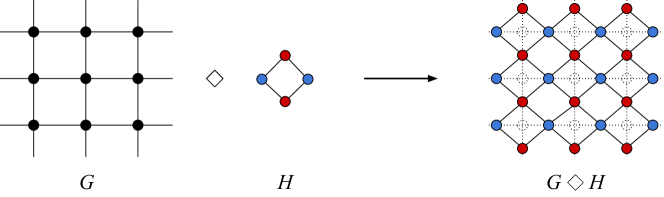
Figure 1: An example of the line product.

Observe that $G\diamond H$ has $nD/2$ vertices and is $2d$-regular. Note also that the line graph of $G$ (where two edges are connected if they share a vertex) is exactly the line product between $G$ and the $D$-clique, hence the name.

The key lemma (Lemma 3.3) is that if $G$ is a small-set (edge) expander and $H$ is a good unique-neighbor expander, then $G\diamond H$ is a unique-neighbor expander as well. For the base graph $G$, we simply use the explicit Ramanujan graph construction [LPS88, Mor94]. For the gadget $H$, we show that a random biregular graph is a good unique-neighbor expander with high probability (Lemma 4.3). Then, since $D$ is a constant, we can find such a graph by brute force.

Remark 1.14 (On importance of Ramanujan base graphs).

We require an $O(\sqrt{D})$ bound on the average degree of small subgraphs in a $D$-regular expander, which is proved using the fact that the second eigenvalue of a $D$-regular Ramanujan graph is $O(\sqrt{D})$. Typically, applications of expanders only need a second eigenvalue bound of $o(D)$, so we find it noteworthy that the analysis of our construction seems to require being within a constant factor of the Ramanujan bound.

Tripartite line product.   Our constructions with stronger vertex expansion guarantees for small sets, featured in Theorem 1.5, are based on a suitably generalized version of the line product, which we call the tripartite line product. The first ingredient is a large tripartite base graph $G$ on vertex set $L\cup M\cup R$, where $L,R,M$ denote the left, middle, right partitions respectively, and there are bipartite graphs between $L$, $M$ and between $M$, $R$. The second ingredient is a small constant-sized bipartite gadget graph $H$, which is chosen to be an excellent unique-neighbor expander — as before, we can brute-force search to find $H$ that has expansion as good as a random graph.

The tripartite line product $G\diamond H$ is a bipartite graph on $L\cup R$ whose edges are obtained by placing a copy of $H$ between the left neighbors of $v$ and the right neighbors of $v$ for each $v\in M$. See Definition 7.6 for a formal definition and Figure 2 for an example.

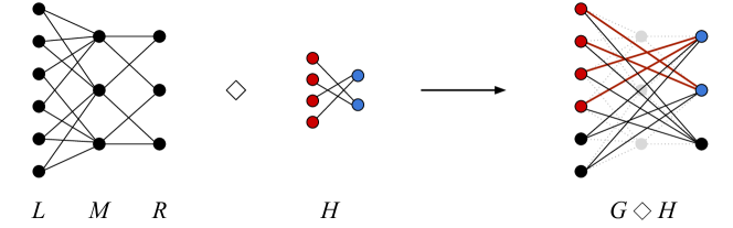
Figure 2: An example of the tripartite line product. The gadget placed on the first vertex in $M$ is highlighted in $G\diamond H$.

To prove Theorem 1.5, we construct the base graph by choosing a $(K_{1},D_{1})$-biregular spectral expander between $L$ and $M$, and a $(D_{2},K_{2})$-biregular spectral expander between $M$ and $R$ for large enough and suitably chosen parameters $K_{1},D_{1},K_{2},D_{2}$. The gadget $H$ is chosen to be a $(\widetilde{d}_{1},\widetilde{d}_{2})$-biregular graph on vertex set $[D_{1}]\times[D_{2}]$, where $d_{1}=K_{1}\widetilde{d}_{1}$ and $d_{2}=K_{2}\widetilde{d}_{2}$.

Remark 1.15 (Generalizing the line product and routed product).

The line product and routed product, which feature in [AC02, AD23, Gol23], arise from instantiating the tripartite line product with appropriate base graphs. The line product can be obtained by choosing a $(2,D_{1})$-biregular graph between $L$ and $M$, and a $(D_{2},2)$-biregular graph between $M$ and $R$ in the base graph. The routed product arises by choosing a $(K,D_{1})$-biregular graph between $L$ and $M$, and a $(D_{2},1)$-biregular graph between $M$ and $R$ in the base graph.

Remark 1.16 (One-sided vs. two-sided expanders).

A key difference between our work and previous constructions that only achieve one-sided expansion is in the choice of the graph between $M$ and $R$. [AD23, Gol23] choose the graph between $M$ and $R$ to be a $(D_{2},1)$-biregular graphs, equivalently a disjoint collection of stars centered at the vertices in $M$. This results in very small sets on the right with no unique-neighbors: for example, for any $v\in M$, consider the set of all its right neighbors.

Overview of the analysis of the tripartite line product.   Let $Z=G\diamond H$, and let $G^{(1)}$ and $G^{(2)}$ be the bipartite graphs between $L,M$ and $M,R$ in $G$ respectively. We choose the gadget $H$ to be a $(\widetilde{d}_{1},\widetilde{d}_{2})$-biregular graph on $D=D_{1}+D_{2}$ vertices such that $\widetilde{d}_{1}\gg\frac{1}{\varepsilon}\sqrt{K_{2}D_{2}}$. For a subset $S\subseteq L$, let $U=N_{G}(S)\subseteq M$ (neighbors of $S$ in the base graph). Our analysis for the expansion of $S$ roughly follows two steps:

1. We partition $U$ according to the number of edges going to $S$ — $U_{\ell}$ (“low $S$-degree”) and $U_{h}$ (“high $S$-degree”). We then show that if we partition $U$ according to a suitable threshold, then most edges leaving $S$ go to $U_{\ell}$.

2. Since each vertex in $U_{\ell}$ has small $S$-degree, in the local gadget graph it has “large” unique-neighbor expansion (here we rely on the expansion profile of the gadget; see Lemma 4.3). Then, we show that most of the unique-neighbors in the gadgets are also unique-neighbors of $S$ in $Z$.

Both steps rely on Theorem 1.11. For step 1, we apply Theorem 1.11 on the induced subgraph $G^{(1)}[S\cup U_{h}]$ (since $G^{(1)}$ is near-Ramanujan). If we choose the threshold to be $\approx\sqrt{D}$, then since the right average degree of $G^{(1)}[S\cup U_{h}]$ is $\gtrsim\sqrt{D}$, the left average degree is $\lesssim 1+\frac{\sqrt{K_{1}D_{1}}}{\sqrt{D}}\ll K_{1}$, thus most edges from $S$ go to $U_{\ell}$ instead of $U_{h}$.

For step 2, let $\widetilde{T}\subseteq R$ be the union of the unique-neighbors within each gadget. By the expansion of the gadgets on vertices in $U_{\ell}$, we have a lower bound on $|\widetilde{T}|$. However, a unique-neighbor in one gadget may also have edges from other gadgets, in which case it is not a unique-neighbor of $S$ in $Z$. To resolve this issue, we analyze the induced subgraph $G^{(2)}[U\cup\widetilde{T}]$ and show that a large fraction of $\widetilde{T}$ are unique-neighbors of $U$ in $G^{(2)}$, thus must also be unique-neighbors of $S$ in $Z$. This is done by observing that the left average degree of $G^{(2)}[U\cup\widetilde{T}]$ must be $\gtrsim\widetilde{d}_{1}$. Thus, the right average degree is $\lesssim 1+\frac{\sqrt{K_{2}D_{2}}}{\widetilde{d}_{1}}\leqslant 1+\varepsilon$ since we choose $\widetilde{d}_{1}\gg\frac{1}{\varepsilon}\sqrt{K_{2}D_{2}}$.

One might attempt to tweak the parameters of the construction to obtain two-sided lossless expansion. However, this fails because in step 1 we need the threshold to be large enough such that $S$ has lossless expansion in $G^{(1)}$, but then it is not possible to set the parameters of the gadget such that (i) each vertex in $U_{\ell}$ expands losslessly, and (ii) $\widetilde{d}_{1}\gg\frac{1}{\varepsilon}\sqrt{K_{2}D_{2}}$ (and $\widetilde{d}_{2}\gg\frac{1}{\varepsilon}\sqrt{K_{1}D_{1}}$) for the analysis in step 2. See Section 7.2 (the proof of Theorem 7.8) for details.

Lossless expansion of small sets.   For small subsets $S\subseteq L$, we directly show that $S$ expands losslessly into $U$ under the assumption that $G^{(1)}$ has no short bicycles. Specifically, in Lemma 7.5 we prove that if a graph has no bicycle of length $g$, then all sufficiently small subsets (in particular, of size at most $\exp(O(g))$) expand losslessly. To prove this, we first show that if a degree-$K$ set $S$ has expansion less than $(1-\varepsilon)K$, then we can lower bound the spectral radius of the non-backtracking matrix of the graph induced on $S\cup N(S)$ by $C(\varepsilon)\coloneqq\sqrt{\varepsilon(K-1)}$. Now, by the generalized Moore bound (Theorem 1.12), there is a bicycle of size $O(\log_{C(\varepsilon)}|S|)$ in $G$. Since $G$ has no bicycle of length-$g$, it lower bounds $|S|$ via the inequality $g\leqslant O(\log_{C(\varepsilon)}|S|)$. This tells us that small sets in $G^{(1)}$ exhibit lossless expansion. To establish that small sets in $Z$ are losslessly expanding, we follow the same strategy as before for step 2: since most vertices in $U$ has only 1 edge to $S$, they expand by a factor of $\widetilde{d}_{1}$ (from the gadget), and we use Theorem 1.11 to show that $T=N_{Z}(S)$ are mostly unique-neighbors, proving the small set expansion result in Theorem 1.5.

One-sided lossless expanders.   As mentioned in Remark 1.7, we are able to use the tripartite line product to construct one-sided lossless expanders, recovering the result of Louis [Gol23]. Our proof is almost the same as Theorem 1.5, but with $K_{1}\gg K_{2}=1$ (hence $G^{(2)}$ is just a collection of stars). In step 1, we choose a smaller $S$-degree threshold $\approx\varepsilon\sqrt{D}$ and large enough $K_{1}$ to ensure that $1-\varepsilon$ fraction of edges from $S$ go to $U_{\ell}$ (via Theorem 1.11). Then, with the smaller threshold, each vertex in $U_{\ell}$ expands losslessly, i.e., by a factor of $(1-\varepsilon)\widetilde{d}_{1}$. Since all gadgets have disjoint right vertices, there is no collision between gadgets, which finishes the proof.

Subgraphs in near-Ramanujan bipartite graphs.   We now give an overview of the proofs of Theorems 1.8 and 1.11. The main ingredient is the Bethe Hessian of a graph $G$ defined as $H_{G}(t)\coloneqq(D_{G}-\mathbbm{1})t^{2}-A_{G}t+\mathbbm{1}$. Specifically, for an induced subgraph $G[S]$, we identify $\alpha>0$ such that $H_{G[S]}(t)\succ 0$ for $t\in[0,\alpha]$ (Theorem 5.1), which then implies Theorem 1.8 via the well-known Ihara–Bass formula (Fact 2.3).

To prove $H_{G[S]}(t)\succ 0$ for $t\in[0,\alpha]$, we show that $f^{\top}H_{G[S]}(t)f>0$ for any $f:G[S]\to\mathbbm{R}$. To establish $f^{\top}H_{G[S]}(t)f>0$ for the claimed values of $t$, we need to relate $f^{\top}H_{G[S]}(t)f$ to the spectrum of the entire graph $G$. To this end, we consider the regular tree extension $T$ of $G[S]$ (Definition 5.6), which is obtained by attaching trees (of depth $\ell$) to each vertex in $S$ such that the resulting graph is $(c,d)$-biregular except for the leaves. Intuitively, the tree extension serves as a proxy of the $\ell$-step neighborhood of $S$ in $G$. We then define the appropriate function extension $f_{t}$ of $f$ (Definition 5.4) on the tree extension with “sufficient decay” down the tree (where the decay results from an upper bound on $t$). For appropriately bounded $t$, we can show $f^{\top}H_{G[S]}(t)f$ is approximately equal to $f_{t}^{\top}H_{G}(t)f_{t}$, which can be controlled via the spectrum of $G$.

Erdős–Rényi vs. random regular graphs.   One technical subtlety is that the edges of a random regular graph are (slightly) correlated, which makes it difficult to directly analyze its unique-neighbor expansion. On the other hand, the analysis is straightforward for Erdős–Rényi graphs since the edges are drawn independently (Lemma B.1).

Thus, we give a slight generalization of an embedding theorem given in [FK16] between Erdős–Rényi graphs and random regular graphs (Lemma B.2) which allows us to extend the analysis to random regular graphs.

1.4 Open questions

Quantum codes from unique-neighbor expanders. Lin & Hsieh [LH22] construct quantum codes assuming the existence of two-sided algebraic lossless expanders, and their current proof requires the unique-neighbor expansion of sets of vertices with degree-$d$ to exceed $d/2$.

In contrast, in the setting of classical LDPC codes, if all subsets of vertices of size at most $\Delta$ have even a single unique-neighbor, the resulting code is guaranteed to have distance at least $\Delta$, albeit without a clear decoding algorithm.

Question 1.17.

Does the construction of [LH22] yield a good quantum code when instantiated with a $\gamma$-two-sided algebraic unique-neighbor expander for small $\gamma>0$?

Algebraic two-sided lossless expanders from random graphs.   Two-sided lossless expanders with relevant algebraic properties are not known to exist, even using randomness. Random bipartite graphs exhibit two-sided lossless expansion (see, for example, [HLW06, Theorem 4.16]), but do not admit any nontrivial group actions.

A natural approach is to use an algebraic random graph, such as a random Cayley graph, and study its vertex expansion properties. It is also possible to achieve lossless expansion using the tripartite line product if the small-set edge expansion of the base graph is far better than that guaranteed by spectral expansion. A concrete question in this direction that could result in a lot of progress is the following.

Question 1.18 (Beyond spectral certificates).

Let $\Gamma$ be a group and let $\bm{S}$ be a set of $D$ generators chosen independently and uniformly from $\Gamma$. Let $\bm{G}\coloneqq\mathrm{Cay}(\Gamma,\bm{S})$ be the Cayley graph given by the generator set $\bm{S}$. Is it true that with high probability over the choice of $\bm{S}$: for all subsets of vertices $T\subseteq\Gamma$ where $|T|\leqslant|\Gamma|/\mathrm{poly}(D)$, the number of edges inside $T$ is at most $0.1\sqrt{D}|T|$?

Remark 1.19.

Spectral expansion can at best guarantee that the number of edges inside a set $T$ is at most $\sqrt{D}|T|$. A resolution to the above question would necessarily use other properties of the random graph and group, beyond merely the magnitude of its eigenvalues.

1.5 Organization

In Section 2, we give some technical preliminaries. In Section 3, we define the line product and prove its unique-neighbor expansion assuming good expansion properties of the base and gadget graphs. In Section 4, we prove Theorem 1.2 by instantiating the line product with a suitably chosen base graph and gadget graph.

In Section 5, we prove Theorem 1.8. In Section 6, we use Theorem 1.8 to prove Theorem 1.11. In Section 7, we define the tripartite line product, and instantiate it with an appropriately chosen base graph and gadget graph to prove Theorem 1.5 via Theorem 1.11 and Theorem 1.12. In Section 8, we show how we can recover Golowich’s [Gol23] construction and analysis of one-sided lossless expanders as an instantiation of the tripartite line product and an application of Theorem 1.11.

In Appendix A, we prove the sharpened Moore bound Theorem 1.12. In Appendices B and C, we analyze the expansion profile of the gadget graph.

2 Preliminaries

Notation.

Given a graph $G$, we use $V(G)$ to denote its set of vertices, $E(G)$ to denote its set of edges. If $G$ is bipartite, we use $L(G)$ and $R(G)$ to denote its left and right vertex sets respectively. We write $\deg_{G}(v)$ to denote the degree of vertex $v$ in $G$ (we will omit the subscript $G$ if clear from context). We say that a bipartite graph $G$ is $(d_{1},d_{2})$-biregular if $\deg_{G}(v)=d_{1}$ for all $v\in L(G)$ and $\deg_{G}(v)=d_{2}$ for all $v\in R(G)$.

For any subset of edges $F$, we use $F(v)\subseteq F$ to denote the set of edges in $F$ incident to $v$, hence $|F(v)|=\deg_{F}(v)$. For a set of vertices $S$, we use $e_{F}(S)$ to denote the number of edges in $F$ with both endpoints in $S$, and $e_{F}(S,T)$ to denote the number of $(u,v)\in S\times T$ such that $\{u,v\}\in F$ (for disjoint sets $S$ and $T$). We will omit the subscript if $F=E(G)$. We denote the eigenvalues of the normalized adjacency matrix of $G$ by $1=\lambda_{1}(G)\geqslant\dots\geqslant\lambda_{n}(G)\geqslant-1$. We say $G$ is a $\lambda$-spectral expander if $\lambda_{2}(G)\leqslant\lambda$.

Random bipartite graph models.

Throughout the paper, we will write random variables in boldface. Fix $n_{1},n_{2},m,d_{1},d_{2}\in\mathbbm{N}$ such that $n_{1}d_{1}=n_{2}d_{2}$. We denote $K_{n_{1},n_{2}}$ as the complete bipartite graph with left/right vertex sets $L=[n_{1}]$ and $R=[n_{2}]$. We use $\bm{G}\sim\mathbb{G}_{n_{1},n_{2},m}$ to denote a random graph sampled from the uniform distribution over (simple) bipartite graphs on $L=[n_{1}]$, $R=[n_{2}]$ with exactly $m$ edges. With slight abuse of notation, we use $\bm{H}\sim\mathbb{G}_{n_{1},n_{2},p}$ for $p\in(0,1)$ to denote a random graph such that each potential edge is included with probability $p$. Similarly, we use $\bm{R}\sim\mathbb{R}_{n_{1},n_{2},d_{1},d_{2}}$ to denote a graph from the uniform distribution over $(d_{1},d_{2})$-biregular bipartite graphs on $L=[n_{1}]$, $R=[n_{2}]$.

2.1 Graph expansion

It is a standard fact that small subgraphs in spectral expanders have bounded number of edges. The following is a special case of the Expander Mixing Lemma [AC88], and we include a short proof for completeness.

Lemma 2.1.

Let $G$ be a $D$-regular $\lambda$-spectral expander. Then for any set $S\subseteq V(G)$, where $|S|=\varepsilon|V(G)|$:

$$e(S)\leqslant D|S|\cdot\frac{\lambda+\varepsilon}{2}\,.$$

Proof.

Let $n=|V(G)|$, $A$ be the (unnormalized) adjacency matrix of $G$, and $\vec{1}_{S}\in\{0,1\}^{n}$ be the indicator vector of $S$. We can decompose $\vec{1}_{S}$ as $\vec{1}_{S}=\frac{|S|}{n}\vec{1}+u$ where $u\perp\vec{1}$ and $\|u\|_{2}^{2}=|S|(1-\frac{|S|}{n})\leqslant|S|$. Then, $2e(S)=\vec{1}_{S}^{\top}A\vec{1}_{S}\leqslant\frac{D|S|^{2}}{n}+\lambda_{2}(G)\cdot D\|u\|_{2}^{2}\leqslant D|S|(\varepsilon+\lambda)$. ∎

Within graphs of low “hereditary” average degree, a significant fraction of edges are incident to low-degree vertices.

Lemma 2.2.

For any $\gamma>0$, let $F$ be a graph such that for all $S\subseteq V(F)$, $2e(S)\leqslant\gamma|S|$. Write $V(F)=F_{\ell}\sqcup F_{h}$ where $F_{\ell}$ comprises all vertices $v$ such that $\deg(v)\leqslant 2\gamma$ and $F_{h}$ to denote the remaining vertices. Then:

$$2e(F)\leqslant 3\sum_{v\in F_{\ell}}\deg(v)\,.$$

Proof.

On one hand, by assumption we have:

$$2e(F_{h})\leqslant\gamma|F_{h}|\,.$$

On the other hand,

$$2e(F_{h})+e(F_{h},F_{\ell})=\sum_{v\in F_{h}}\deg(v)\geqslant 2\gamma|F_{h}|\geqslant 4e(F_{h})\,.$$

Consequently $e(F_{h},F_{\ell})\geqslant 2e(F_{h})$. Since $F_{h}$ and $F_{\ell}$ are disjoint:

$$2e(F)=2e(F_{h})+e(F_{h},F_{\ell})+e(F_{\ell},F_{h})+2e(F_{\ell})\,.$$

This gives us: $2e(F)\leqslant 3e(F_{h},F_{\ell})+2e(F_{\ell})\leqslant 3\sum_{v\in F_{\ell}}\deg(v)\,.$ ∎

2.2 Non-backtracking matrix

Notation.

Given an undirected graph $G=(V,E)$ with $|V|=n$ vertices and $|E|=m$ edges, we denote $A_{G}\in\{0,1\}^{n\times n}$ to be its adjacency matrix, $D_{G}\in\mathbbm{R}^{n\times n}$ to be its diagonal degree matrix, and finally $B_{G}\in\{0,1\}^{2m\times 2m}$ to be its non-backtracking matrix (introduced by [Has89]) defined as follows: for directed edges $(u_{1},v_{1}),(u_{2},v_{2})$ in the graph,

$$B_{G}[(u_{1},v_{1}),(u_{2},v_{2})]=\bm{1}(v_{1}=u_{2})\cdot\bm{1}(u_{1}\neq v_{2})\,.$$

Note that the non-backtracking matrix is not symmetric. Let $\lambda_{1},\dots,\lambda_{2m}\in\mathbbm{C}$ be the eigenvalues of $B_{G}$ ordered such that $|\lambda_{1}|\geqslant|\lambda_{2}|\geqslant\cdots\geqslant|\lambda_{2m}|$. The Perron-Frobenius theorem implies that $\lambda_{1}$ is real and non-negative. We denote $\rho(B_{G})=\lambda_{1}$ to be the spectral radius of $B_{G}$.

A crucial identity we will need is the Ihara-Bass formula [Iha66, Bas92] which gives a translation between the eigenvalues of the adjacency matrix and the eigenvalues of the non-backtracking matrix:

Fact 2.3 (Ihara-Bass formula).

For any graph $G$ with $n$ vertices and $m$ edges, the following identity on univariate polynomials is true:

$$\det\left\lparen\mathbbm{1}-B_{G}t\right\rparen=\det\left\lparen H_{G}(t)\right\rparen\cdot(1-t^{2})^{m-n}$$

where $H_{G}(t)\coloneqq(D_{G}-\mathbbm{1})t^{2}-A_{G}t+\mathbbm{1}$ is the Bethe Hessian of $G$.

The Ihara-Bass formula gives a direct relationship between the spectral radius of $B_{G}$ and the positive definiteness of $H_{G}(t)$. The following is classic (e.g. [FM17, Proof of Theorem 5.1]), though we include a proof for completeness.

Lemma 2.4.

Let $G$ be a graph and $0<\alpha<1$. Then, the spectral radius $\rho(B_{G})\leqslant\frac{1}{\alpha}$ if and only if $H_{G}(t)\succ 0$ for all $t\in[0,\alpha)$. As a result, if $H_{G}(\frac{1}{\rho})$ has a non-positive eigenvalue for some $\rho>0$, then $\rho(B_{G})\geqslant\rho$.

Proof.

First observe that $H_{G}(0)=\mathbbm{1}\succ 0$. Since $H_{G}(t)$ is symmetric, the eigenvalues of $H_{G}(t)$ are real and move continuously on the real line as $t$ increases from $0$. Note also that by the Perron-Frobenius theorem, $\rho(B_{G})=\lambda_{1}(B_{G})\geqslant 0$.

Suppose for contradiction that $\rho(B_{G})\leqslant\frac{1}{\alpha}$ but $H_{G}(t)$ has a non-positive eigenvalue for some $t\in[0,\alpha)$. Due to $H_{G}(0)=\mathbbm{1}$ and continuity of the eigenvalues, there must be a $t^{*}\in(0,t]$ such that $H_{G}(t^{*})$ has a zero eigenvalue, meaning $\det(H_{G}(t^{*}))=0$. By Fact 2.3, this means that $\det(\mathbbm{1}-B_{G}t^{*})=0$, i.e., $B_{G}$ has an eigenvalue $\frac{1}{t^{*}}\geqslant\frac{1}{t}>\frac{1}{\alpha}$. This contradicts that $\rho(B_{G})\leqslant\frac{1}{\alpha}$.

On the other hand, if $H_{G}(t)\succ 0$ for all $t\in[0,\alpha)$, then by Fact 2.3 $\det(\mathbbm{1}-B_{G}t)>0$ for all $t\in[0,\alpha)$. Since $\det(\mathbbm{1}-B_{G}/\lambda_{1})=0$, it follows that $\frac{1}{\lambda_{1}}\geqslant\alpha$, i.e., $\lambda_{1}\leqslant\frac{1}{\alpha}$.

Finally, suppose $H_{G}(\frac{1}{\rho})\not\succ 0$ for some $\rho>0$, then setting $\alpha=\frac{1}{\rho-\varepsilon}>\frac{1}{\rho}$ for any $\varepsilon\to 0^{+}$, we have that $\rho(B_{G})>\rho-\varepsilon$. This implies that $\rho(B_{G})\geqslant\rho$. ∎

3 The line product of graphs

Our construction is based on taking the line product of a suitably chosen spectral expander and unique-neighbor expander. See Figure 1 for an example.

Definition 3.1 (Line product).

Let $G$ be a $D$-regular graph on vertex set $[n]$, and let $H$ be a graph on vertex set $[D]$. For each $v\in V(G)$ and $i\in[D]$, let $e_{v}^{i}$ denote the $i$-th incident edge to $v$. The line product $G\diamond H$ is the graph on vertex set $E(G)$ and edges obtained by placing a copy of $H$ on $E(v)$ for each $v\in V(G)$, such that $\{e_{v}^{i},e_{v}^{j}\}$ is an edge in $H(v)$ if and only if $\{i,j\}$ is an edge in $H$.

For convenience, we denote $H(v)$ to be the subgraph of $G\diamond H$ given by the copy of $H$ associated with $v$.

Definition 3.2.

Given a graph $H$, we denote $\mathrm{UN}_{H}(S)$ to be the set of unique-neighbors of $S$. The unique-neighbor expansion profile of a graph $H$, denoted $P_{H}$, is defined:

$$P_{H}(t)\coloneqq\min_{S\subseteq V(H):|S|\leqslant t}\frac{|\mathrm{UN}_{H}(S)|}{|S|}\quad\textnormal{for $t\geqslant 1$}.$$

When $H$ is a bipartite graph, we use $P_{H}^{(L)}(t)$ and $P_{H}^{(R)}(t)$ to denote the analogous quantity where the minimum is taken only over subsets of the left and right respectively.

Lemma 3.3 (Expansion profile of the line product).

Let $\gamma>0$ and $\varepsilon\in(0,1)$. Suppose

1. $G$ is a $D$-regular graph such that $2e(S)\leqslant\gamma|S|$ for all $S\subset V(G)$ with $|S|\leqslant\varepsilon|V(G)|$, and

2. $H$ is a graph on $[D]$ such that $P_{H}(t)\geqslant 12\gamma/t$ for $1\leqslant t\leqslant 2\gamma$.

Then for $Z\coloneqq G\diamond H$, $P_{Z}\left({\frac{\varepsilon}{D}}\cdot|V(Z)|\right)\geqslant\frac{P_{H}(2\gamma)}{3}$.

Proof.

Let $T\subseteq V(Z)$, viewed as a collection of edges in $G$, be such that $|T|\leqslant{\frac{\varepsilon}{D}}\cdot|V(Z)|=\frac{\varepsilon}{2}\cdot|V(G)|$ (since $|V(Z)|=|E(G)|=\frac{D}{2}|V(G)|$). Let $S\subseteq V(G)$ be the set of vertices of $G$ touched by $T$. Note that $|S|\leqslant 2|T|\leqslant\varepsilon|V(G)|$. Recall that we denote $T(v)\subseteq T$ to be the set of edges in $T$ incident to $v$, and we have $\deg_{T}(v)=|T(v)|\leqslant\deg_{G[S]}(v)$. Then,

$$\left\lvert\mathrm{UN}_{Z}(T)\right\rvert=\sum_{v\in S}\left\lvert\mathrm{UN}_{H(v)}(T(v))\right\rvert-\sum_{v\in S}\sum_{\begin{subarray}{c}v^{\prime}\in S\\ v\neq v^{\prime}\end{subarray}}\left\lvert\mathrm{UN}_{H(v)}(T(v))\cap\mathrm{UN}_{H(v^{\prime})}(T(v^{\prime}))\right\rvert\,.$$

Each summand in the first term of the right-hand side can be lower bounded using $P_{H}$ (see below). A vertex $\{v_{1},v_{2}\}\in V(Z)$ (an edge in $G$) is contained in exactly two subgraphs $H(v_{1})$ and $H(v_{2})$, so it can only be counted twice in the second term, which means we can bound the whole sum by $2e(S)$.

Since $|S|\leqslant\varepsilon|V(G)|$, by the assumption on $G$, both the induced subgraph $G[S]$ and $T$ (viewed as a subgraph of $G[S]$) satisfy the assumption of Lemma 2.2, i.e., all $S^{\prime}\subseteq S$ satisfies $2e_{T}(S^{\prime})\leqslant 2e(S^{\prime})\leqslant\gamma|S^{\prime}|$. Thus, define $S_{1}\coloneqq\{v\in S:\deg_{T}(v)\leqslant 2\gamma\}$ and $S_{2}\coloneqq\{v\in S:\deg_{G[S]}(v)\leqslant 2\gamma\}\subseteq S_{1}$. Applying Lemma 2.2 to both $T$ and $G[S]$, we get that $2|T|=2e_{T}(S)\leqslant 3\sum_{v\in S_{1}}\deg_{T}(v)$ and $2e(S)\leqslant 3\sum_{v\in S_{2}}\deg_{G[S]}(v)\leqslant 6\gamma|S_{2}|\leqslant 6\gamma|S_{1}|$, hence

$$\left\lvert\mathrm{UN}_{Z}(T)\right\rvert \geqslant\sum_{v\in S}|T(v)|\cdot P_{H}\left\lparen|T(v)|\right\rparen-2e(S)$$

$$\geqslant\sum_{v\in S}|T(v)|\cdot P_{H}\left\lparen|T(v)|\right\rparen-6\gamma|S_{1}|$$

$$=\sum_{v\in S_{1}}|T(v)|\cdot\left\lparen P_{H}\left\lparen|T(v)|\right\rparen-\frac{6\gamma}{|T(v)|}\right\rparen+\sum_{v\in S\setminus S_{1}}|T(v)|\cdot P_{H}\left\lparen|T(v)|\right\rparen$$

$$\geqslant\frac{1}{2}\sum_{v\in S_{1}}|T(v)|\cdot P_{H}\left\lparen|T(v)|\right\rparen\,,$$

where the last inequality is by $|T(v)|=\deg_{T}(v)\leqslant 2\gamma$ for all $v\in S_{1}$ and the assumption that $P_{H}(t)\geqslant 12\gamma/t$ for all $t\leqslant 2\gamma$. Then since $P_{H}(t)$ is monotonically decreasing with $t$ and $\sum_{v\in S_{1}}|T(v)|\geqslant\frac{2}{3}|T|$,

$$\frac{\left\lvert\mathrm{UN}_{Z}(T)\right\rvert}{|T|}\geqslant\frac{1}{2|T|}\sum_{v\in S_{1}}|T(v)|\cdot P_{H}(2\gamma)\geqslant\frac{P_{H}(2\gamma)}{3}\,.\qed$$

4 Algebraic unique-neighbor expanders

We use a Ramanujan graph equipped with symmetries bestowed by its Cayley graph structure as our base spectral expander.

Fact 4.1 (Ramanujan graph construction [LPS88, Mor94]).

For every $D=p^{r}+1$ where $p$ is prime and $r\in\mathbbm{N}$, there is an infinite family of groups $(\Gamma_{n})_{n\in\mathbbm{N}}$ and a collection of generators $A\subseteq\Gamma_{n}$ closed under inversion where $|A|=D$ such that the Cayley graph $G\coloneqq\mathrm{Cay}(\Gamma_{n},A)$ is a $D$-regular Ramanujan graph, i.e., it is a $\frac{2\sqrt{D-1}}{D}$-spectral expander.

For arbitrary $D$, by deleting a few edges, we can get $D$-regular Cayley graphs that satisfy the expanding condition in Lemma 3.3 with similar parameters as Ramanujan graphs.

Lemma 4.2 (Expanding Cayley graphs of every degree).

For every $D\in\mathbbm{N}$, $D\geqslant 3$, there is an infinite family of groups $(\Gamma_{n})_{n\in\mathbbm{N}}$ and a collection of generators $A\subseteq\Gamma_{n}$ closed under inversion where $|A|=D$ such that the Cayley graph $G\coloneqq\mathrm{Cay}(\Gamma_{n},A)$ is a $D$-regular graph such that

$$2e(S)\leqslant 3D|S|\left(\frac{2\sqrt{D-1}}{D}+\varepsilon\right),\quad\forall S\subseteq V(G),\ |S|=\varepsilon|V(G)|.$$

Proof.

For odd $D$, there exists an $r\in\mathbbm{N}$ such that $D-1\leqslant 2^{r}\leqslant 2(D-1)$, thus we set $D^{\prime}=2^{r}+1\leqslant 2D$. For even $D$, there exists an $r\in\mathbbm{N}$ such that $D-1\leqslant 3^{r}\leqslant 3(D-1)$, thus we set $D^{\prime}=3^{r}+1\leqslant 3D$. We construct the $D^{\prime}$-regular graph $G^{\prime}=\mathrm{Cay}(\Gamma_{n},A^{\prime})$ via Fact 4.1 such that $\lambda_{2}(G^{\prime})\leqslant\frac{2\sqrt{D^{\prime}-1}}{D^{\prime}}\leqslant\frac{2\sqrt{D-1}}{D}$ (since $\frac{2\sqrt{x-1}}{x}$ is decreasing with $x$ for $x\geqslant 2$).

Since $D$ and $D^{\prime}$ have the same parity, we can remove pairs of generators $g\neq g^{-1}$ from $A^{\prime}$ until there are $D$ elements left (if at some point only self-inverse elements remain, then we start removing them one at a time). Let $A$ be the remaining generators with $|A|=D$. By construction, $G\coloneqq\mathrm{Cay}(\Gamma_{n},A)$ is $D$-regular.

Now, we upper bound $e(S)$. Deleting edges can only decrease $e(S)$, so by Lemma 2.1,

$$2e(S)\leqslant D^{\prime}|S|(\lambda_{2}(G^{\prime})+\varepsilon)\leqslant 3D|S|\left(\frac{2\sqrt{D-1}}{D}+\varepsilon\right).$$

This completes the proof. ∎

For the gadget, we will need a unique-neighbor expander with strong quantitative guarantees.

Lemma 4.3.

Let $\beta\in(0,1/2]$, $\theta>0$, and $\tau>0$ be constants. For integers $d_{1},d_{2},D_{1},D_{2}$ and $D\coloneqq D_{1}+D_{2}$ satisfying

1. $\frac{d_{1}}{d_{2}}=\frac{D_{2}}{D_{1}}$,

2. $1\geqslant\frac{d_{1}}{d_{2}}\geqslant\frac{\beta}{1-\beta}$,

3. $\theta\sqrt{D}/2\leqslant d_{1}+d_{2}\leqslant\theta\sqrt{D}$,

there is a $(d_{1},d_{2})$-biregular graph $H$ with $D_{1}$ vertices on the left and $D_{2}$ vertices on the right such that:

$$P_{H}(t)\geqslant(1-o_{D}(1))\cdot d_{1}\cdot\exp(-\theta t/\sqrt{D})$$

for $1\leqslant t\leqslant\tau\sqrt{D}$ where $o_{D}(1)$ hides constant factors depending only on $\beta,\theta$ and $\tau$.

We defer the proof of Lemma 4.3 to Appendix B, and prove our main theorem below.

Theorem 4.4 (Formal version of Theorem 1.2).

For every $\beta\in(0,1/2]$, there are $d_{0}=d_{0}(\beta)>0$ and $\delta=\delta(\beta)>0$ such that for all even $d_{1},d_{2}\geqslant d_{0}$ with $1\geqslant\frac{d_{1}}{d_{2}}\geqslant\frac{\beta}{1-\beta}$, there is an infinite family of $(2d_{1},2d_{2})$-biregular graphs $(Z_{n})_{n\geqslant 1}$ with

$$\left\lvert\mathrm{UN}_{Z_{n}}(S)\right\rvert\geqslant\delta\cdot d_{1}\cdot|S|,\quad\forall S\subseteq V(Z_{n})\text{ with }|S|\leqslant\frac{1}{d_{1}^{3}}\cdot\left\lvert V\left\lparen Z_{n}\right\rparen\right\rvert\,.$$

Proof.

The construction of $Z_{n}$ is based on taking the line product of $G_{n}$ from Fact 4.1 and a bipartite gadget graph $H$ from Lemma 4.3 for suitably chosen parameters.

Fix parameters $\tau=18$, $\theta=\frac{40\tau}{\beta}$, and choose $d_{0}$ to be large enough such that $d_{0}\geqslant\frac{8}{\beta}e^{\tau\theta}$ and such that for $D\geqslant 4d_{0}^{2}/\theta^{2}$, the $o_{D}(1)$ terms in Lemma 4.3 and all subsequent occurrences in this proof are smaller than $0.1$. For $d_{1},d_{2}\geqslant d_{0}$, let $D_{1}\coloneqq\left\lceil\frac{d_{1}+d_{2}}{\theta^{2}}\right\rceil\cdot d_{2}$ and $D_{2}\coloneqq\left\lceil\frac{d_{1}+d_{2}}{\theta^{2}}\right\rceil\cdot d_{1}$, and define $D\coloneqq D_{1}+D_{2}$. This choice of parameters satisfies the requirements of Lemma 4.3, and hence there is a $(d_{1},d_{2})$-biregular graph $H$ with $D_{1}$ left vertices, $D_{2}$ right vertices, and

$$P_{H}(t)\geqslant 0.9\cdot d_{1}\cdot\exp(-\theta t/\sqrt{D})$$

for $t\leqslant\tau\sqrt{D}$.

We choose $G_{n}$ as an $n$-vertex $D$-regular expander graph from Lemma 4.2. It remains to prove that $Z_{n}=G_{n}\diamond H$ has the claimed unique-neighbor expansion guarantee, and is indeed a $(2d_{1},2d_{2})$-biregular graph (which requires an appropriate ordering of $H$).

Note that by Lemma 4.2, $G_{n}$ satisfies $2e(S)\leqslant 9\sqrt{D}\cdot|S|$ for all $S\subseteq V(G_{n})$ with $|S|\leqslant\frac{1}{\sqrt{D}}n$, which satisfies the first condition in Lemma 3.3 with $\varepsilon=\frac{1}{\sqrt{D}}$ and $\gamma=9\sqrt{D}=\frac{\tau}{2}\sqrt{D}$. Thus, it suffices to show that $P_{H}(t)$ satisfies the second condition in Lemma 3.3 (a weaker lower bound):

$$(\ref{eq:PH-lower-bound})\geqslant\frac{12\gamma}{t}=\frac{6\tau\sqrt{D}}{t},\quad\textnormal{ for }1\leqslant t\leqslant 2\gamma=\tau\sqrt{D}\,.$$ (3)

This allows us to apply Lemma 3.3 and the (stronger) lower bound of $P_{H}(t)$ in Section 4 to get

$$P_{Z_{n}}\left(\frac{1}{D^{3/2}}\cdot|V(Z_{n})|\right)\geqslant\frac{1}{3}P_{H}(\tau\sqrt{D})\geqslant 0.3e^{-\tau\theta}\cdot d_{1}\coloneqq\delta\cdot d_{1}$$

for constant $\delta=0.3e^{-\tau\theta}$. Since $D\leqslant\frac{4}{\theta^{2}}(d_{1}+d_{2})^{2}$, $\beta(d_{1}+d_{2})\leqslant d_{1}$, and $\beta\theta=40\tau$, we have $\frac{1}{D^{3/2}}\geqslant\frac{1}{d_{1}^{3}}$. As $P_{Z_{n}}(t)$ is a decreasing function with $t$, this establishes the desired unique-neighbor expansion as articulated in Theorem 4.4, finishing the proof of the theorem.

Now, to establish Eq. 3, observe that the function $xe^{-x}$ is monotone increasing for $x\leqslant 1$ and monotone decreasing for $x\geqslant 1$, hence for $x\in[a,b]$, $xe^{-x}\geqslant\min\{ae^{-a},be^{-b}\}$. Thus, for $1\leqslant t\leqslant\tau\sqrt{D}$,

$$\frac{\theta t}{\sqrt{D}}\cdot e^{-\theta t/\sqrt{D}}\geqslant\min\left\{\frac{\theta}{\sqrt{D}}\cdot e^{-\theta/\sqrt{D}},\ \tau\theta\cdot e^{-\tau\theta}\right\}.$$

By using $d_{1}\geqslant\beta(d_{1}+d_{2})$, $d_{1}+d_{2}\geqslant\theta\sqrt{D}/2$ and the above, from Section 4 we get $P_{H}(t)\geqslant\frac{\sqrt{D}}{t}\cdot 0.45\beta\theta\cdot\min\{e^{-\theta/\sqrt{D}},\tau\sqrt{D}\cdot e^{-\tau\theta}\}$.

With our choice of parameters, $\beta\theta\geqslant 40\tau$ and $\sqrt{D}\geqslant 2d_{0}/\theta\geqslant\theta$ imply that $0.45\beta\theta\cdot e^{-\theta/\sqrt{D}}\geqslant 6\tau$. Furthermore, $\theta\sqrt{D}\geqslant d_{1}+d_{2}\geqslant 2d_{0}\geqslant\frac{16}{\beta}e^{\tau\theta}$ implies that $0.45\beta\theta\cdot\tau\sqrt{D}e^{-\tau\theta}\geqslant 6\tau$. Therefore, we have established Eq. 3.

Finally, we show that $Z_{n}$ is a $(2d_{1},2d_{2})$-biregular graph. Since $G_{n}=\mathrm{Cay}(\Gamma,A)$ is a Cayley graph with generators $A$, each edge $\{u,v\}$ is labeled by group elements $a$ and $a^{-1}$ in $A$, i.e., $\{u,v\}=e_{u}^{a}=e_{v}^{a^{-1}}$. To construct the line product $G_{n}\diamond H$, we need a bijective map $\varphi$ between $A$ and $V(H)=L(H)\cup R(H)$ such that each pair $a,a^{-1}\in A$ gets assigned to the same side of $H$. This can be done as long as $d_{1}$ and $d_{2}$ are even.

Let $L(Z_{n})=\{e_{v}^{a}:v\in V(G_{n}),\ \varphi(a)\in L(H)\}$ and $R(Z_{n})=\{e_{v}^{a}:v\in V(G_{n}),\ \varphi(a)\in R(H)\}$. First, $L(Z_{n})$ and $R(Z_{n})$ is a disjoint partition of $E(G_{n})=V(Z_{n})$ since $a,a^{-1}$ are assigned to the same side of $H$. Moreover, all edges of $Z_{n}$ are between $L(Z_{n})$ and $R(Z_{n})$, establishing bipartiteness of $Z_{n}$. Finally, observe that the degree of $e\in V(Z_{n})$, an edge between $u$ and $v$, is $d_{1}$ in both $H(u)$ and $H(v)$ if $e\in L(Z_{n})$, and $d_{2}$ in both if $e\in R(Z_{n})$, which implies $(2d_{1},2d_{2})$-biregularity. ∎

5 Non-backtracking matrix of subgraphs

In this section, we bound the spectral radius of the nonbacktracking matrix of subgraphs of bipartite spectral expanders. This gives us tight control over the degree profile of subgraphs, improving on bounds provided by classic tools like the expander mixing lemma [AC88].

The following is a generalization of an analogous result of Kahale for regular graphs [Kah95, Theorem 1].

Theorem 5.1 (Formal version of Theorem 1.8).

Let $\varepsilon\in(0,0.1)$, and let $3\leqslant c\leqslant d$ be integers. Let $G=(L\cup R,E)$ be a $(c,d)$-biregular graph and $S\subseteq L\cup R$ such that $|S|\leqslant d^{-1/\varepsilon}|L\cup R|$. Then, for any $t\geqslant 0$ such that

$$\frac{1}{t}\geqslant\frac{1}{2}\left(\sqrt{\widetilde{\lambda}^{2}-(\sqrt{c-1}+\sqrt{d-1})^{2}}+\sqrt{\widetilde{\lambda}^{2}-(\sqrt{c-1}-\sqrt{d-1})^{2}}\right)\,,$$ (4)

where $\widetilde{\lambda}=\max(\lambda_{2}(A_{G}),\sqrt{c-1}+\sqrt{d-1})\cdot(1+O(\varepsilon))$, we have

$$H_{G[S]}(t)\succ 0\,.$$

To understand Eq. 4, consider $\widetilde{\lambda}\approx\sqrt{c-1}+\sqrt{d-1}$. Then, Eq. 4 simplifies to $\frac{1}{t}\gtrsim((c-1)(d-1))^{1/4}$. More specifically, suppose $\widetilde{\lambda}=(\sqrt{c-1}+\sqrt{d-1})(1+\gamma/d)$, then denoting $\eta\coloneqq(\sqrt{c-1}+\sqrt{d-1})^{2}(\frac{2\gamma}{d}+\frac{\gamma^{2}}{d^{2}})$, Eq. 4 becomes $\frac{1}{t}\geqslant\sqrt{\sqrt{(c-1)(d-1)}+\eta/4}+\frac{1}{2}\sqrt{\eta}$. In particular, we have the following corollary.

Corollary 5.2.

Let $3\leqslant c\leqslant d$, and suppose $\widetilde{\lambda}=(\sqrt{c-1}+\sqrt{d-1})(1+\gamma/d)$ for $\gamma\in[0,2]$, then

$$\frac{1}{t^{2}}\geqslant\sqrt{(c-1)(d-1)}\cdot(1+3\sqrt{\gamma})$$

implies Eq. 4.

Overview of the proof.   We prove $H_{G[S]}(t)\succ 0$ by showing that $\langle f,H_{G[S]}(t)f\rangle>0$ for all $f:S\to\mathbbm{R}$. The way we prove $\langle f,H_{G[S]}(t)f\rangle>0$ is by relating it to a quadratic form against the matrix $H_{G}(t)$, which we can control via the spectrum of $G$. In particular, we consider the depth-$\ell$ regular tree extension $T$ of $G[S]$, and for $f$ we define an appropriate function extension $f_{t}$ on the tree depending on $t$ (Definition 5.4) such that $\langle f,H_{G[S]}(t)f\rangle=\langle f_{t},H_{T}(t)f_{t}\rangle$. The function $f_{t}$ additionally has the property that its $\ell_{2}$ mass on vertices $r$-far from $G[S]$ decays exponentially in $r$. At a high level, we use the tree extension as a proxy for the $\ell$-step neighborhood of $S$ in $G$, and this is made precise in Section 5.3 as we define a natural folded function $\widetilde{f}_{t}$ of $f_{t}$ into $G$ (Definition 5.9).

This allows us to lower bound $\langle f,H_{G[S]}(t)f\rangle$ by $\langle\widetilde{f}_{t},H_{G}(t)\widetilde{f}_{t}\rangle$ with some errors. The errors can be bounded using the decay of $f_{t}$ from the definition, though this requires $t<((c-1)(d-1))^{-1/4}$ (see Lemma 5.7). Ignoring errors, it comes down to showing that

$$\frac{1}{t^{4}}-\frac{1}{t^{2}}\left(\lambda^{2}-(c-1)-(d-1)\right)+(c-1)(d-1)>0\,,$$

and we solve the quadratic formula in Lemma 5.12 and show that the above gives rise to Eq. 4. The full proof is presented in Section 5.4.

5.1 Tree extensions

We start with defining tree extensions of a graph.

Definition 5.3 (Tree extension).

For a graph $G=(V,E)$, we say that $T=(V(T),E(T))$ is a tree extension of $G$ if $T$ is obtained by attaching a tree $T_{r}$ to each vertex $r\in V$, with $r$ being the root. Each vertex $x\in T$ belongs to a unique tree $T_{r}$ rooted at $r$. For any $x\in T$, we write $0pt(x)$ to be the distance between $x$ and the root of the tree containing $x$.

Fix a tree extension $T$ of $G$, for functions $f,g:V(T)\to\mathbbm{R}$, define $\langle f,g\rangle=\sum_{x\in T}f(x)g(x)$ and $\lVert f\rVert_{2}^{2}=\sum_{x\in T}f(x)^{2}$.

Definition 5.4 (Function extension).

Given a function $f:V(G)\to\mathbbm{R}$, a tree extension $T$ of $G$, and parameter $t\in\mathbbm{R}$, we define $f_{t}:V(T)\to\mathbbm{R}$ to be the extension of $f$ to $T$ such that for $x\in T$,

$$f_{t}(x)=f(r)\cdot t^{0pt(x)},\quad\text{if }x\in T_{r}\,.$$ (5)

The following simple but crucial lemma establishes a relationship between $H_{G}$ and $H_{T}$, which also motivates the definition of $f_{t}$.

Lemma 5.5.

Let $G$ be a graph and $T$ be any tree extension of $G$. Then, for any $t\in\mathbbm{R}$ and $f:V(G)\to\mathbbm{R}$, the extension $f_{t}:V(T)\to\mathbbm{R}$ defined in Eq. 5 satisfies

$$\left(H_{T}(t)\cdot f_{t}\right)(x)=\begin{cases}(H_{G}(t)\cdot f)(x)&x\in V(G)\,,\\ 0&x\notin V(G)\,.\end{cases}$$

Proof.

Recall that $H_{G}(t)=(D_{G}-\mathbbm{1})t^{2}-A_{G}t+\mathbbm{1}$. For $x\notin V(G)$, let $d(x)$ be its degree and let $r\in V(G)$ be the root of the tree containing $x$. Observe that $x$ has 1 parent (with value $f(r)t^{0pt(x)-1}$) and $d(x)-1$ children (with value $f(r)t^{0pt(x)+1}$) in the tree $T_{r}$. Thus,

$$\left(H_{T}(t)\cdot f_{t}\right)(x) =((d(x)-1)t^{2}+1)\cdot f(r)t^{0pt(x)}-t\cdot f(r)\left(t^{0pt(x)-1}+(d(x)-1)t^{0pt(x)+1}\right)$$

$$=0\,.$$

For $x\in V(G)$, let $d_{G}(x)$ be its degree in $G$ and $d_{T}(x)$ be its degree in $T$. Then, $x$ has $d_{T}(x)-d_{G}(x)$ children (with value $t\cdot f(x)$) in the tree $T_{x}$.

$$\left(H_{T}(t)\cdot f_{t}\right)(x) =((d_{T}(x)-1)t^{2}+1)\cdot f(x)-t\Big{(}(A_{G}f)(x)+(d_{T}(x)-d_{G}(x))\cdot tf(x)\Big{)}$$

$$=((d_{G}(x)-1)t^{2}+1)\cdot f(x)-t(A_{G}f)(x)$$

$$=(H_{G}(t)\cdot f)(x)\,.$$

This completes the proof. ∎

5.2 Regular tree extensions of subgraphs

For a subgraph $G[S]$ in a regular (or biregular) graph, we consider its regular tree extension.

Definition 5.6 (Regular tree extension).

Let $G=(V,E)$ be a $d$-regular graph, $S\subseteq V$, $\ell\in\mathbbm{N}$, and consider the induced subgraph $G[S]$. We define the depth-$\ell$ regular tree extension of $G[S]$ to be the tree extension $T$ of $G[S]$ where depth-$\ell$ trees are attached to vertices in $S$ such that the resulting graph is $d$-regular except for the leaves. Let $\mathsf{Leaves}(T)$ denote the set of leaves.

Similarly, let $G=(L\cup R,E)$ be a $(c,d)$-biregular graph, $S\subseteq L\cup R$, and $\ell\in\mathbbm{N}$. The depth-$\ell$ regular tree extension of $G[S]$ is the tree extension such that the resulting graph is $(c,d)$-biregular except for the leaves.

We show that given a graph $G=(V,E)$ and $S\subseteq V$, for any function $f:S\to\mathbbm{R}$ and its extension $f_{t}$ to the depth-$\ell$ regular tree extension of $G[S]$, the contribution from the leaves decays exponentially with $\ell$ when $t<((c-1)(d-1))^{-1/4}$.

Lemma 5.7 (Decay of $f_{t}$).

Let $G=(L\cup R,E)$ be a $(c,d)$-biregular graph with $c\leqslant d$, let $S\subseteq L\cup R$, let $\ell\in\mathbbm{N}$ be even, and let $T$ be the depth-$\ell$ regular tree extension of $G[S]$. Moreover, let $t\in\mathbbm{R}$ such that $t^{2}\sqrt{(c-1)(d-1)}=1-\delta$ for some $\delta\in(0,1)$. Given any function $f:S\to\mathbbm{R}$, let $f_{t}:V(T)\to\mathbbm{R}$ be the function extension (as defined in Eq. 5), and let $f_{t}^{=\ell}$ be $f_{t}$ restricted to the leaves of $T$. Then,

$$\left\lVert f_{t}^{=\ell}\right\rVert_{2}^{2}\leqslant\frac{2\delta}{e^{\delta\ell}-1}\cdot\left\lVert f_{t}\right\rVert_{2}^{2}\,.$$

Since the function $\frac{2x}{e^{x\ell}-1}$ is monotone decreasing, we have for any $\delta^{\prime}>\delta$,

$$\left\lVert f_{t}^{=\ell}\right\rVert_{2}^{2}\leqslant\frac{2\delta^{\prime}}{e^{\delta^{\prime}\ell}-1}\cdot\left\lVert f_{t}\right\rVert_{2}^{2}\,.$$

Proof.

We will lower bound $\left\lVert f_{t}\right\rVert_{2}^{2}$ and upper bound the contribution from the leaves at depth $\ell$. Fix a vertex $r\in R$ (with $\deg_{G}(r)=d$) and consider the tree $T_{r}$ rooted at $r$. Let $\deg_{T_{r}}(r)$ be the degree of $r$ in $T_{r}$. The number of children of vertices in the tree alternates between $c-1$ and $d-1$ as we go down the tree. Thus, for an even integer $k\leqslant\ell$, the number of vertices in the $k$-th level is

$$\deg_{T_{r}}(r)(c-1)\left((c-1)(d-1)\right)^{\frac{k}{2}-1}=\frac{\deg_{T_{r}}(r)}{\deg_{G}(r)-1}\left((c-1)(d-1)\right)^{\frac{k}{2}}\,.$$ (6)

The same argument shows that the above also holds for $r\in L$ (with $\deg_{G}(r)=c$). Thus, the contribution of the tree $T_{r}$ to $\left\lVert f_{t}\right\rVert_{2}^{2}$ can be lower bounded by the product of the following two terms:

$$f(r)^{2}\frac{\deg_{T_{r}}(r)}{\deg_{G}(r)-1}$$

$$\sum_{\begin{subarray}{c}0\leqslant k\leqslant\ell\\ \text{$k$ even}\end{subarray}}t^{2k}((c-1)(d-1))^{\frac{k}{2}}= \sum_{i=0}^{\ell/2}(1-\delta)^{2i}=\frac{1-(1-\delta)^{\ell+2}}{1-(1-\delta)^{2}}\geqslant\frac{1-(1-\delta)^{\ell}}{2\delta}\,.$$

Next, the contribution from the leaves of $T_{r}$ to $\left\lVert f_{t}^{=\ell}\right\rVert_{2}^{2}$ is also given by Eq. 6. Thus, we have

$$\frac{\left\lVert f_{t}^{=\ell}\right\rVert_{2}^{2}}{\left\lVert f_{t}\right\rVert_{2}^{2}}\leqslant(1-\delta)^{\ell}\frac{2\delta}{1-(1-\delta)^{\ell}}\leqslant\frac{2\delta}{e^{\delta\ell}-1}\,,$$

using $(1-\delta)^{\ell}\leqslant e^{-\delta\ell}$, finishing the proof. ∎

5.3 Folding regular tree extensions

Given a regular tree extension $T$ of an induced subgraph $G[S]$, there is a natural folding into $G$ via breadth-first search from $S$.

Definition 5.8 (Folding into $G$).

Let $G=(V,E)$ be a $d$-regular or $(c,d)$-biregular graph, let $S\subseteq V$, and let $T$ be the depth-$\ell$ regular tree extension of $G[S]$. There is a natural homomorphism $\sigma:T\to G$ such that

• $\sigma(x)=x$ for all $x\in S$;

• $\deg_{T}(x)=\deg_{G}(\sigma(x))$ for all $x\in V(T)\setminus\mathsf{Leaves}(T)$;

• Two edges $\{x,y\}$ and $\{y,z\}$ in $T$ sharing a vertex are not mapped to the same edge in $E$, i.e., all edges in $T$ that map to the same edge in $E$ are vertex-disjoint.

Definition 5.9 (Folded function).

Fix a map $\sigma:T\to G$. Given any $f:V(T)\to\mathbbm{R}$, we associate each vertex $v\in G$ with a function $f^{v}:V(T)\to\mathbbm{R}$ such that for $x\in T$,

$$f^{v}(x)=\begin{cases}f(x)&\text{if $\sigma(x)=v$}\,,\\ 0&\text{otherwise}\,.\end{cases}$$

We define the folded function $\widetilde{f}:V(G)\to\mathbbm{R}$ to be

$$\widetilde{f}(v)=\left\lVert f^{v}\right\rVert_{2}\,.$$

Observation 5.10.

The $f^{v}$’s have disjoint support, thus $\lVert\widetilde{f}\rVert_{2}^{2}=\sum_{v\in G}\lVert f^{v}\rVert_{2}^{2}=\lVert f\rVert_{2}^{2}$. More generally, let $\Gamma,\widetilde{\Gamma}$ be diagonal operators such that $(\Gamma f)(x)=\gamma(\deg_{G}(\sigma(x)))f(x)$ for $x\in T$ and $(\widetilde{\Gamma}g)(v)=\gamma(\deg_{G}(v))g(v)$ for $v\in G$. Then, $\langle\widetilde{f},\widetilde{\Gamma}\widetilde{f}\rangle=\langle f,\Gamma f\rangle$.

We next prove the following useful lemma that relates the quadratic forms of $f$ and $\widetilde{f}$ with $A_{G}$.

Lemma 5.11.

Let $G=(V,E)$ be a $d$-regular or $(c,d)$-biregular graph, let $S\subseteq V$, and let $T$ be a regular tree extension of $G[S]$. For any $f:V(T)\to\mathbbm{R}$ and its folded function $\widetilde{f}:V(G)\to\mathbbm{R}$, we have

$$\left\langle f,A_{T}f\right\rangle\leqslant\left\langle\widetilde{f},A_{G}\widetilde{f}\right\rangle\,.$$

Proof.

Recall from Definition 5.8 that the map $\sigma:T\to G$ satisfies that if $\{x,y\}$ is an edge in $T$, then $\{\sigma(x),\sigma(y)\}\in E$. Then,

$$\left\langle f,A_{T}f\right\rangle=2\sum_{\{x,y\}\in E(T)}f(x)f(y)=2\sum_{\{u,v\}\in E(G)}\sum_{\{x,y\}\in E(T)}\bm{1}(\sigma(\{x,y\})=\{u,v\})\cdot f^{\sigma(x)}(x)f^{\sigma(y)}(y)\,.$$

Moreover, all edges in $T$ that map to the same edge are vertex-disjoint. Thus, for any $\{u,v\}\in E$, $\sum_{\{x,y\}\in E(T)}\bm{1}(\sigma(\{x,y\})=\{u,v\})\cdot f^{\sigma(x)}(x)f^{\sigma(y)}(y)$ can be expressed as an inner product between some permutations of $f^{u}$ and $f^{v}$, which is upper bounded by $\lVert f^{u}\rVert_{2}\cdot\lVert f^{v}\rVert_{2}=\widetilde{f}(u)\widetilde{f}(v)$ by Cauchy-Schwarz. Thus, we have

$$\left\langle f,A_{T}f\right\rangle\leqslant 2\sum_{\{u,v\}\in E(G)}\widetilde{f}(u)\widetilde{f}(v)=\left\langle\widetilde{f},A_{G}\widetilde{f}\right\rangle\,.\qed$$

5.4 Proof of Theorem 5.1

Before we prove Theorem 5.1, we first prove the following lemma for convenience.

Lemma 5.12.

Let $3\leqslant c\leqslant d\in\mathbbm{N}$ and $\varepsilon\in(0,1)$. Let $\lambda\geqslant\sqrt{c-1}+\sqrt{d-1}$ and $\widetilde{\lambda}=\lambda(1+\varepsilon)$. Then, for all $x$ such that

$$x\geqslant\frac{1}{2}\left(\sqrt{\widetilde{\lambda}^{2}-(\sqrt{c-1}+\sqrt{d-1})^{2}}+\sqrt{\widetilde{\lambda}^{2}-(\sqrt{c-1}-\sqrt{d-1})^{2}}\right)\,,$$

we have

$$x^{4}-x^{2}(\lambda^{2}(1+\varepsilon)-(c+d-2))+(c-1)(d-1)>0\,.$$

Proof.

Denote $a\coloneqq c-1$ and $b\coloneqq d-1$ for convenience. Then, to show that $x^{4}-x^{2}(\lambda^{2}(1+\varepsilon)-a-b)+ab\geqslant 0$, it suffices to verify that

$$x^{2}>\frac{1}{2}\left(\lambda^{2}(1+\varepsilon)-a-b\right)+\frac{1}{2}\sqrt{\left(\lambda^{2}(1+\varepsilon)-a-b\right)^{2}-4ab}\,.$$

Squaring both sides of $x\geqslant\frac{1}{2}\Big{(}\sqrt{\widetilde{\lambda}^{2}-(\sqrt{a}+\sqrt{b})^{2}}+\sqrt{\widetilde{\lambda}^{2}-(\sqrt{a}-\sqrt{b})^{2}}\Big{)}$, we get

$$x^{2} \geqslant\frac{1}{2}\left(\widetilde{\lambda}^{2}-a-b\right)+\frac{1}{2}\sqrt{(\widetilde{\lambda}^{2}-(\sqrt{a}+\sqrt{b})^{2})(\widetilde{\lambda}^{2}-(\sqrt{a}-\sqrt{b})^{2})}$$

$$=\frac{1}{2}\left(\widetilde{\lambda}^{2}-a-b\right)+\frac{1}{2}\sqrt{\widetilde{\lambda}^{4}-2(a+b)\widetilde{\lambda}^{2}+(a-b)^{2}}$$

$$=\frac{1}{2}\left(\widetilde{\lambda}^{2}-a-b\right)+\frac{1}{2}\sqrt{(\widetilde{\lambda}^{2}-a-b)^{2}-4ab}\,,$$

which completes the proof with $\widetilde{\lambda}=\lambda(1+\varepsilon)$. ∎

Proof of Theorem 5.1.

We first verify that the assumption on $t$ (Eq. 4) implies that

$$t^{2}\leqslant\frac{1-\varepsilon}{\sqrt{(c-1)(d-1)}}\,.$$ (7)

Indeed, as $\widetilde{\lambda}=\lambda(1+O(\varepsilon))\geqslant(\sqrt{c-1}+\sqrt{d-1})(1+\varepsilon)$, Eq. 4 implies that

$$\frac{1}{t^{2}} \geqslant\frac{1}{4}\left((\sqrt{c-1}+\sqrt{d-1})^{2}(1+\varepsilon)^{2}-(\sqrt{c-1}-\sqrt{d-1})^{2}\right)$$

$$\geqslant\sqrt{(c-1)(d-1)}+\frac{1}{2}(\sqrt{c-1}+\sqrt{d-1})^{2}\varepsilon$$

which implies Eq. 7.

We would like to show that $\langle f,H_{G[S]}(t)f\rangle>0$ for any function $f:S\to\mathbbm{R}$. Let $\ell=\lceil\frac{1}{2\varepsilon}\rceil$ be an even integer and let $T$ be the depth-$\ell$ regular tree extension of $G[S]$ (Definition 5.6). Let $f_{t}:V(T)\to\mathbbm{R}$ be the function extension of $f$ to $T$ with parameter $t$. By Lemma 5.5, we have

$$\left\langle f,H_{G[S]}(t)f\right\rangle=\left\langle f_{t},H_{T}(t)f_{t}\right\rangle=\left\langle f_{t},((D_{T}-\mathbbm{1})t^{2}-tA_{T}+\mathbbm{1})f_{t}\right\rangle\,.$$

Note that all internal vertices $x\in T\setminus\mathsf{Leaves}(T)$ have degree $c$ or $d$ while the leaves have degree $1$. Let $D_{T}^{\prime}$ be the diagonal matrix such that the leaves have the “correct” degree, i.e., for $x\in\mathsf{Leaves}(T)$ in the tree $T_{r}$ rooted at $r\in S$, $D_{T}^{\prime}[x,x]=\deg_{G}(r)$ (since $\ell$ is even). Then, by Eq. 7, Lemma 5.7 states that $f_{t}^{=\ell}$ decays with a factor $\frac{2\varepsilon}{e^{\varepsilon\ell}-1}\leqslant 4\varepsilon$, thus

$$\left\langle f_{t},(D_{T}-\mathbbm{1})f_{t}\right\rangle=\left\langle f_{t},(D_{T}^{\prime}-\mathbbm{1})f_{t}\right\rangle-\left\langle f_{t}^{=\ell},(D_{T}^{\prime}-\mathbbm{1})f_{t}^{=\ell}\right\rangle\geqslant\left\langle f_{t},(D_{T}^{\prime}-\mathbbm{1})f_{t}\right\rangle\left(1-4\varepsilon\right)\,.$$

Consider the folded function $\widetilde{f}_{t}:V(G)\to\mathbbm{R}$ as defined in Definition 5.9. By 5.10, we have $\left\langle f_{t},D_{T}^{\prime}f_{t}\right\rangle=\langle\widetilde{f}_{t},D_{G}\widetilde{f}_{t}\rangle$ and $\lVert f_{t}\rVert_{2}^{2}=\lVert\widetilde{f}_{t}\rVert_{2}^{2}$. Moreover, by Lemma 5.11, $\langle f_{t},A_{T}f_{t}\rangle\leqslant\left\langle\widetilde{f}_{t},A_{G}\widetilde{f}_{t}\right\rangle$. Thus,

$$\left\langle f,H_{G[S]}(t)f\right\rangle \geqslant t^{2}\left\langle\widetilde{f}_{t},(D_{G}-\mathbbm{1})\widetilde{f}_{t}\right\rangle(1-4\varepsilon)-t\left\langle\widetilde{f}_{t},A_{G}\widetilde{f}_{t}\right\rangle+\left\lVert\widetilde{f}_{t}\right\rVert_{2}^{2}$$

$$\geqslant(1-4\varepsilon)\left\langle\widetilde{f}_{t},\left(t^{2}(D_{G}-\mathbbm{1})+\mathbbm{1}\right)\widetilde{f}_{t}\right\rangle-t\left\langle\widetilde{f}_{t},A_{G}\widetilde{f}_{t}\right\rangle\,.$$ (8)

We would like to show that the above is non-negative. Denote $\Gamma_{G}\coloneqq t^{2}(D_{G}-\mathbbm{1})+\mathbbm{1}$, and $\gamma_{1}\coloneqq t^{2}(c-1)+1$ and $\gamma_{2}\coloneqq t^{2}(d-1)+1$. Note that $\gamma_{2}\geqslant\gamma_{1}>0$ as we assume that $c\leqslant d$. Since $G$ is a $(c,d)$-biregular graph, $\Gamma_{G}$ and $A_{G}$ have the following block structure,

$$\Gamma_{G}=\begin{pmatrix}\gamma_{1}\mathbbm{1}&0\\ 0&\gamma_{2}\mathbbm{1}\end{pmatrix}\,,\quad A_{G}=\begin{pmatrix}0&A_{L,R}\\ A_{L,R}^{\top}&0\end{pmatrix}\,.$$

In particular,

$$(1-4\varepsilon)\Gamma_{G}-tA_{G}=\Gamma_{G}^{1/2}\left((1-4\varepsilon)\mathbbm{1}-t\cdot\Gamma_{G}^{-1/2}A_{G}\Gamma_{G}^{-1/2}\right)\Gamma_{G}^{1/2}=\Gamma_{G}^{1/2}\left((1-4\varepsilon)\mathbbm{1}-\frac{t}{\sqrt{\gamma_{1}\gamma_{2}}}A_{G}\right)\Gamma_{G}^{1/2}\,.$$

Then, denoting $g\coloneqq\Gamma_{G}^{1/2}\widetilde{f}_{t}$, we can write Eq. 8 as

$$\left\langle f,H_{G[S]}(t)f\right\rangle\geqslant\left\langle\widetilde{f}_{t},\left((1-4\varepsilon)\Gamma_{G}-tA_{G}\right)\widetilde{f}_{t}\right\rangle=(1-4\varepsilon)\left\lVert g\right\rVert_{2}^{2}-\frac{t}{\sqrt{\gamma_{1}\gamma_{2}}}\left\langle g,A_{G}g\right\rangle\,.$$ (9)

Next, we upper bound $\langle g,A_{G}g\rangle$. For any $(c,d)$-biregular graph, the (normalized) top eigenvector of $A_{G}$ is $\frac{1}{\sqrt{2|E|}}D_{G}^{1/2}\vec{1}$ with eigenvalue $\sqrt{cd}$. Thus,

$$\left\langle g,A_{G}g\right\rangle\leqslant\frac{\sqrt{cd}}{2|E|}\left\langle g,D_{G}^{1/2}\vec{1}\right\rangle^{2}+\lambda\left\lVert g\right\rVert_{2}^{2}\,,$$

where $\lambda=\max(\lambda_{2}(A_{G}),\sqrt{c-1}+\sqrt{d-1})$ is the second eigenvalue.

Since $T$ has depth $\ell$, the support of $\widetilde{f}_{t}$ (and $g$) must be contained in $B\coloneqq\{v\in V(G):\mathrm{dist}(v,S)\leqslant\ell\}$. We have $|B|\leqslant|S|\sum_{i=0}^{\ell}d^{i}\leqslant|S|d^{\ell+1}$. Thus, by Cauchy-Schwarz,

$$\frac{\sqrt{cd}}{2|E|}\left\langle g,D_{G}^{1/2}\vec{1}\right\rangle^{2}\leqslant\frac{\sqrt{cd}}{2|E|}\cdot d|B|\cdot\left\lVert g\right\rVert_{2}^{2}\leqslant d^{-1/4\varepsilon}\left\lVert g\right\rVert_{2}^{2}\leqslant\varepsilon\left\lVert g\right\rVert_{2}^{2}\,,$$

since $|S|\leqslant d^{-1/\varepsilon}|L\cup R|$, $\ell=\lceil\frac{1}{2\varepsilon}\rceil$, $|E|=c|L|=d|R|$, and $\varepsilon\leqslant 0.1$ (note that $d^{-1/4\varepsilon}\leqslant\varepsilon$ for all $d\geqslant 3$ and $\varepsilon\leqslant 0.1$).

Thus, $\langle g,A_{G}g\rangle\leqslant(\lambda+\varepsilon)\left\lVert g\right\rVert_{2}^{2}\leqslant\lambda(1+\varepsilon)\left\lVert g\right\rVert_{2}^{2}$, and from Eq. 9,

$$\left\langle f,H_{G[S]}(t)f\right\rangle\geqslant\frac{1}{\sqrt{\gamma_{1}\gamma_{2}}}\left((1-4\varepsilon)\sqrt{\gamma_{1}\gamma_{2}}-t\lambda(1+\varepsilon)\right)\,.$$

As $\frac{1+\varepsilon}{1-4\varepsilon}\leqslant 1+5\varepsilon$, to prove that the above is positive, it suffices to prove that $t^{2}\lambda^{2}(1+5\varepsilon)<\gamma_{1}\gamma_{2}=(t^{2}(c-1)+1)(t^{2}(d-1)+1)$, or equivalently,

$$\frac{1}{t^{4}}-\frac{1}{t^{2}}\left(\lambda^{2}(1+5\varepsilon)-(c-1)-(d-1)\right)+(c-1)(d-1)>0\,.$$

With $\widetilde{\lambda}=\lambda(1+5\varepsilon)$ and the assumption on $t$ (Eq. 4), the above holds via Lemma 5.12. ∎

6 Expansion and density of subgraphs

The spectral radius of the nonbacktracking matrix of a subgraph of a bipartite graph imposes constraints on the left and right degrees, articulated by the following.

Theorem 6.1 (Subgraph density in (near-)Ramanujan graphs; restatement of Theorem 1.11).

Let $3\leqslant c\leqslant d$ be integers, $\gamma\in[0,1]$, and $\varepsilon\in(0,0.1)$. Let $G=(L\cup R,E)$ be a $(c,d)$-biregular graph such that $\lambda_{2}(G)\leqslant(\sqrt{c-1}+\sqrt{d-1})(1+\gamma/d)$. Then, there exists $\delta=\delta(\varepsilon,c,d)>0$ such that for every $S_{1}\subseteq L$ and $S_{2}\subseteq R$ with $|S_{1}|+|S_{2}|\leqslant\delta|L\cup R|$, the left and right average degrees $d_{1}=\frac{|E(S_{1},S_{2})|}{|S_{1}|}$ and $d_{2}=\frac{|E(S_{1},S_{2})|}{|S_{2}|}$ in the induced subgraph $G[S_{1}\cup S_{2}]$ must satisfy

$$(d_{1}-1)(d_{2}-1)\leqslant\sqrt{(c-1)(d-1)}\cdot(1+O(\varepsilon+\sqrt{\gamma}))\,.$$

Theorem 6.1 is a direct consequence of Theorem 5.1 and the following lemma:

Lemma 6.2.

Let $G=(L\cup R,E)$ be a bipartite graph, and let the left and right average degrees be $d_{1}=\frac{|E|}{|L|}$ and $d_{2}=\frac{|E|}{|R|}$, respectively. Then, for any $t\in(-1,1)\setminus\{0\}$ such that $H_{G}(t)\succeq 0$, we have

$$(d_{1}-1)(d_{2}-1)\leqslant\frac{1}{t^{2}}\,.$$

Proof.

We can assume that $d_{1},d_{2}>1$, otherwise the statement holds trivially with $|t|<1$. Let $x$ be the vector such that for $u\in L\cup R$,

$$x_{u}=\begin{cases}1&u\in L,\\ \alpha&u\in R,\end{cases}$$

where $\alpha\in\mathbbm{R}$ will be determined later. Recall that $H_{G}(t)=(D_{G}-\mathbbm{1})t^{2}-tA_{G}+\mathbbm{1}$. Since $|E|=d_{1}|L|=d_{2}|R|$, we have $x^{\top}D_{G}x=d_{1}|L|+\alpha^{2}d_{2}|R|=(1+\alpha^{2})d_{1}|L|$ and $x^{\top}A_{G}x=2\alpha|E|=2\alpha d_{1}|L|$, and substituting $|R|=\frac{d_{1}}{d_{2}}|L|$ we get

$$x^{\top}H_{G}(t)x =x^{\top}\left((D_{G}-\mathbbm{1})t^{2}-tA_{G}+\mathbbm{1}\right)x$$

$$=t^{2}\left((d_{1}-1)|L|+\alpha^{2}(d_{2}-1)|R|\right)-t\cdot 2\alpha d_{1}|L|+\left(|L|+\alpha^{2}|R|\right)$$

$$=|L|\left((d_{1}-1)t^{2}-2t\alpha d_{1}+1\right)+|R|\left(\alpha^{2}(d_{2}-1)t^{2}+\alpha^{2}\right)$$

$$=|L|\left((d_{1}-1)t^{2}+\alpha^{2}d_{1}t^{2}-2t\alpha d_{1}+1+\frac{d_{1}}{d_{2}}\cdot\alpha^{2}(1-t^{2})\right)\,.$$

Then, $H_{G}(t)\succeq 0$ and $t\in(-1,1)$ imply that

$$\frac{1}{d_{2}}\geqslant\frac{1}{1-t^{2}}\left(-\frac{(d_{1}-1)t^{2}+1}{d_{1}\alpha^{2}}+\frac{2t}{\alpha}-t^{2}\right)\,.$$

To maximize the right-hand side, we choose $\frac{1}{\alpha}=\frac{d_{1}t}{(d_{1}-1)t^{2}+1}$, which gives

$$\frac{1}{d_{2}}\geqslant\frac{1}{1-t^{2}}\left(\frac{d_{1}t^{2}}{(d_{1}-1)t^{2}+1}-t^{2}\right)=\frac{1}{1-t^{2}}\cdot\frac{t^{2}(d_{1}-1)(1-t^{2})}{(d_{1}-1)t^{2}+1}=\frac{1}{1+\frac{1}{(d_{1}-1)t^{2}}}$$

$$\implies d_{2}\leqslant 1+\frac{1}{(d_{1}-1)t^{2}}\,.$$

Rearranging the above gives $(d_{1}-1)(d_{2}-1)\leqslant 1/t^{2}$. ∎

We can now prove Theorem 6.1.

Proof of Theorem 6.1.

We consider the induced subgraph $G[S_{1}\cup S_{2}]$. By Theorem 5.1, we can choose $t$ such that $\frac{1}{t^{2}}\approx\sqrt{(c-1)(d-1)}$ and $H_{G[S_{1}\cup S_{2}]}(t)\succeq 0$ — specifically, set $\delta=d^{-d/\varepsilon^{2}}$ (depending only on $\varepsilon,d$) and $\widetilde{\lambda}=(\sqrt{c-1}+\sqrt{d-1})(1+\gamma/d)\cdot(1+O(\varepsilon^{2}/d))$, then by Corollary 5.2, $H_{G[S_{1}\cup S_{2}]}\succeq 0$ as long as

$$\frac{1}{t^{2}}\geqslant\sqrt{(c-1)(d-1)}\cdot\left(1+O\left(\sqrt{\gamma+\varepsilon^{2}}\right)\right)=\sqrt{(c-1)(d-1)}\left(1+O(\varepsilon+\sqrt{\gamma})\right)\,.$$

Plugging the above into Lemma 6.2 completes the proof. ∎

As a corollary of Theorem 6.1, we recover the following result of Asherov and Dinur [AD23] proved for Ramanujan graphs, which further extends to near-Ramanujan graphs.

Corollary 6.3.

Let $3\leqslant c\leqslant d$ be integers, $\gamma\in[0,1]$, and $\varepsilon\in(0,0.1)$. Let $G=(L\cup R,E)$ be a $(c,d)$-biregular graph such that $\lambda_{2}(G)\leqslant(\sqrt{c-1}+\sqrt{d-1})(1+\gamma/d)$. Then, there exists $\delta=\delta(\varepsilon,c,d)>0$ such that for every $S\subseteq L$ of size $|S|\leqslant\delta|L|$,

$$\frac{c|S|}{|N(S)|}\leqslant 1+(1+O(\varepsilon+\sqrt{\gamma}))\sqrt{\frac{d-1}{c-1}}\,.$$

7 Unique-neighbor expanders with lossless small-set expansion

In this section, we prove Theorem 1.5.

Theorem (Restatement of Theorem 1.5).

For every $\beta\in(0,1/2]$ and $\varepsilon>0$, there are constants $\gamma>0$ and $K$ such that for all large enough $d_{1},d_{2}$ with $1\geqslant\frac{d_{1}}{d_{2}}\geqslant\frac{\beta}{1-\beta}$ that are multiples of $K$, there is an explicit infinite family of $(d_{1},d_{2})$-biregular graphs $(Z_{n})_{n\geqslant 1}$ where:

1. $Z_{n}$ is a $\gamma$-two-sided unique-neighbor expander,

2. every $S\subseteq L(Z_{n})$ with $|S|\leqslant\exp(\Omega(\sqrt{\log|V(Z_{n})|}))$ has $(1-\varepsilon)\cdot d_{1}\cdot|S|$ unique-neighbors,

3. every $S\subseteq R(Z_{n})$ with $|S|\leqslant\exp(\Omega(\sqrt{\log|V(Z_{n})|}))$ has $(1-\varepsilon)\cdot d_{2}\cdot|S|$ unique-neighbors.

The graphs from Theorem 1.5 are constructed by taking the tripartite line product of a tripartite graph on vertex set $L\cup M\cup R$ where $L\cup M$ and $M\cup R$ are (different) near-Ramanujan biregular graphs with no short bicycles, with suitably chosen degrees. In particular, from the works of [MOP20, OW20], we have the following.

Theorem 7.1 (Special case of main theorem in [OW20]).

For every $c,d\geqslant 3$ and $\gamma>0$, there is an explicit construction of an infinite family of $(c,d)$-biregular graphs $(G_{n})_{n\geqslant 1}$ where $\lambda_{2}(G_{n})\leqslant(\sqrt{c-1}+\sqrt{d-1})\cdot(1+\gamma)$, and $G_{n}$ has no bicycle on $o(\sqrt{\log|V(G_{n})|})$ vertices.

Theorem 1.5 is then a consequence of choosing the graphs between $L$ & $M$, and $M$ & $R$ using the above theorem in conjunction with the forthcoming Theorem 7.8.

Remark 7.2.

Replacing the above choice of base graph with one equipped with a group action and improved bicycle-free radius would result in a group action for the construction in Theorem 1.5 as well as improved parameters. It is plausible that the construction of [BFG⁺15] satisfies these properties, but we do not prove it in this work.

7.1 Lossless expansion in high-girth graphs

We first define the notion of bicycles from [MOP20].

Definition 7.3 (Excess).

Given a graph $G=(V,E)$, its excess is $\operatorname{exc}(G)=|E|-|V|$. In particular, a graph with excess $0$ and $1$ is called cyclic and bicyclic respectively.

We will also need the following refinement of the well-known irregular Moore bound for graphs.

Theorem 7.4 (Generalized Moore bound; formal version of Theorem 1.12).

Suppose $G$ is a graph on $n$ vertices, and let $\rho=\lambda_{1}(B_{G})$ be the spectral radius of its non-backtracking matrix $B_{G}$. Suppose $\rho>1$, then $G$ contains a cycle of size at most $2(\lfloor\log_{\rho}n\rfloor+1)$ and a bicycle of size at most $3(\lfloor\log_{\rho}2n\rfloor+1)$.

We defer the proof of Theorem 7.4 to Appendix A. As mentioned in Remark 1.13, for a graph $G$ with average degree $d$, $\rho(B_{G})$ is at least $d-1$. This follows from the fact that $\vec{1}^{\top}H_{G}(\frac{1}{d-1})\vec{1}=0$ and Lemma 2.4. Therefore, Theorem 7.4 (the cycle case) is potentially stronger than the girth guarantee of $2\log_{d-1}n$ from the classical Moore bound.

Finally, we will need the following statement about the expansion of small sets in graphs with no short cycles or bicycles, which generalizes [Kah95, Theorem 10].

Lemma 7.5 (Expansion of small sets).

Let $G=(L\cup R,E)$ be a $d$-left-regular bipartite graph, and let $\varepsilon\in(0,1)$ such that $\varepsilon(d-1)>1$. Suppose $G$ has no cycle of length at most $g$, then for all $S\subseteq L$ with $|S|\leqslant\frac{1}{d+1}(\varepsilon(d-1))^{\frac{1}{4}g-\frac{1}{2}}$ we have $|N_{G}(S)|\geqslant(1-\varepsilon)d|S|$.

Similarly, suppose $G$ has no bicycle of length at most $g$, then for all $S\subseteq L$ with $|S|\leqslant\frac{1}{2(d+1)}(\varepsilon(d-1))^{\frac{1}{6}g-\frac{1}{2}}$ we have $|N_{G}(S)|\geqslant(1-\varepsilon)d|S|$.

Proof.

Let $T\coloneqq N_{G}(S)\subseteq R$. Suppose $S$ does not expand losslessly, i.e., $|T|<(1-\varepsilon)d|S|$. Then, the subgraph $G[S\cup T]$ must have right average degree at least $\frac{d|S|}{(1-\varepsilon)d|S|}\geqslant\frac{1}{1-\varepsilon}\geqslant 1+\varepsilon$. Let $\rho>0$ be the spectral radius of the non-backtracking matrix $B_{G[S\cup T]}$ so that $H_{G[S\cup T]}(1/\rho)\succeq 0$. Then, applying Lemma 6.2, we have

$$1+\varepsilon\leqslant 1+\frac{\rho^{2}}{(d-1)}\implies\rho\geqslant\sqrt{\varepsilon(d-1)}\,.$$

Next, by Theorem 7.4, $G[S\cup T]$ must contain a cycle of size at most

$$2\log_{\rho}(|S|+|T|)+2\leqslant\frac{2\log((d+1)|S|)}{\log\sqrt{\varepsilon(d-1)}}+2\,.$$

Suppose $|S|\leqslant\frac{1}{d+1}(\varepsilon(d-1))^{\frac{1}{4}(g-2)}$, then there exists a cycle of length at most $g$, which is a contradiction.

Similarly, by Theorem 7.4, $G[S\cup T]$ must contain a bicycle of size at most

$$3\log_{\rho}(2(|S|+|T|))+3\leqslant\frac{3\log(2(d+1)|S|)}{\log\sqrt{\varepsilon(d-1)}}+3\,.$$

Suppose $|S|\leqslant\frac{1}{2(d+1)}(\varepsilon(d-1))^{\frac{1}{6}(g-3)}$, then there exists a bicycle of length at most $g$, which is a contradiction. ∎

7.2 Tripartite line product

We now define a generalization of the line product.

Definition 7.6 (Tripartite line product).

Let $G=(L\cup M\cup R,E_{1}\cup E_{2})$ be a tripartite graph consisting of a $(K_{1},D_{1})$-biregular graph $G^{(1)}=(L\cup M,E_{1})$ and a $(D_{2},K_{2})$-biregular graph $G^{(2)}=(M\cup R,E_{2})$. Let $H$ be a bipartite graph on vertex set $[D_{1}]\cup[D_{2}]$. The tripartite line product $G\diamond H$ is the bipartite graph on vertex set $L\cup R$ and edges obtained by placing a copy of $H$ on the neighbors of $v$ for each $v\in M$.

Remark 7.7.

Note that Definition 7.6 is indeed a generalization of the line product in Definition 3.1 (where $H$ is bipartite). To see this, consider a $D$-regular graph $G$ and define a tripartite graph $G^{\prime}$ as follows: set $M=V(G)$, set $L,R$ to be a partition of $E(G)$, and for $v\in M$ and $e=L\cup R$, connect $\{v,e\}$ if and only if $v\in e$. Note that in this case $K_{1}=K_{2}=2$. If $L,R$ satisfy that each $v\in M$ has $D_{1}$ neighbors in $L$ and $D_{2}$ neighbors in $R$ (with $D=D_{1}+D_{2}$), then $G^{\prime}\diamond H$ is exactly the same as $G\diamond H$ in Definition 3.1.

We now prove Theorem 1.5; we use the tripartite line product to construct two-sided unique-neighbor expanders where we can additionally guarantee that small enough sets expand losslessly.

Theorem 7.8 (Formal version of Theorem 1.5).

Suppose for some $c,d\geqslant 3$ and all $\gamma>0$, there exists an explicit infinite family of $(c,d)$-biregular near-Ramanujan graphs $(F_{n})_{n\geqslant 1}$ with $\lambda_{2}(F_{n})\leqslant(\sqrt{c-1}+\sqrt{d-1})(1+\gamma)$ and has no bicycle of size at most $g_{n}=\omega_{n}(1)$.

For every $\beta\in(0,1/2]$ and $\varepsilon\in(0,1)$, there are $K=K(\varepsilon)$, $d_{0}=d_{0}(\beta,\varepsilon)$ and $\delta=\delta(\beta,\varepsilon)>0$ such that for all $d_{1},d_{2}\geqslant d_{0}$ which are multiples of $K$ and satisfy $1\geqslant\frac{d_{1}}{d_{2}}\geqslant\frac{\beta}{1-\beta}$, the following holds: there exists $\mu=\mu(\beta,\varepsilon,d_{1},d_{2})>0$ such that there is an infinite family of $(d_{1},d_{2})$-biregular graphs $(Z_{n})_{n\geqslant 1}$ where

$$\left\lvert\mathrm{UN}_{Z_{n}}(S)\right\rvert\geqslant\delta\cdot d_{1}\cdot|S|\,,\quad\forall S\subseteq V(Z_{n})\text{ with }|S|\leqslant\mu\cdot\left\lvert V(Z_{n})\right\rvert\,.$$

Moreover,

$$\left\lvert N_{Z_{n}}(S)\right\rvert\geqslant(1-\varepsilon)\cdot d_{1}\cdot|S|\,,\quad\forall S\subseteq L(Z_{n})\text{ with }|S|\leqslant\exp(g_{n})\,,$$

$$\left\lvert N_{Z_{n}}(S)\right\rvert\geqslant(1-\varepsilon)\cdot d_{2}\cdot|S|\,,\quad\forall S\subseteq R(Z_{n})\text{ with }|S|\leqslant\exp(g_{n})\,.$$

Proof.

The construction of $Z_{n}$ is based on taking the tripartite line product of some $G_{n}$ and a bipartite gadget graph $H$ from Lemma 4.3 with suitably chosen parameters.

• Let $K=K_{1}=K_{2}=\frac{1000}{\varepsilon^{2}}$.

• Let $d_{0}\geqslant C_{0}K$ where $C_{0}=C_{0}(\varepsilon,\beta)$ is some large enough constant chosen later.

• Let $\widetilde{d}_{1}\coloneqq d_{1}/K$ and $\widetilde{d}_{2}\coloneqq d_{2}/K$, both at least $C_{0}$.

• Let $\theta\coloneqq\frac{C}{\varepsilon}\sqrt{K/\beta}$ (depending only on $\varepsilon,\beta$) where $C$ is a universal constant.

• Let $D_{1}\coloneqq\left\lceil\frac{\widetilde{d}_{1}+\widetilde{d}_{2}}{\theta^{2}}\right\rceil\cdot\widetilde{d}_{2}$ and $D_{2}\coloneqq\left\lceil\frac{\widetilde{d}_{1}+\widetilde{d}_{2}}{\theta^{2}}\right\rceil\cdot\widetilde{d}_{1}$, and define $D\coloneqq D_{1}+D_{2}$.

Note that $1\geqslant\widetilde{d}_{1}/\widetilde{d}_{2}=d_{1}/d_{2}\geqslant\frac{\beta}{1-\beta}$. One can verify that $KD_{1}\leqslant 2\varepsilon^{2}\widetilde{d}_{2}^{2}/C^{2}$ and $KD_{2}\leqslant 2\varepsilon^{2}\widetilde{d}_{1}^{2}/C^{2}$.

The above choice of parameters satisfy the requirements of Lemma 4.3. Thus, applying Lemma 4.3 with parameters $\theta$ and $\tau=1$, there is a $(\widetilde{d}_{1},\widetilde{d}_{2})$-biregular graph $H$ with $D_{1}$ left vertices and $D_{2}$ right vertices such that

$$\min_{S\subseteq V(H):1\leqslant|S|\leqslant t}\frac{|\mathrm{UN}_{H}(S)|}{|S|}\geqslant(1-o_{D}(1))\cdot\widetilde{d}_{1}\cdot\exp(-\theta t/\sqrt{D})$$ (10)

for $1\leqslant t\leqslant\sqrt{D}$. We can set $C_{0}$ large enough (depending only on $\beta,\theta$ which only depend on $\varepsilon,\beta$) such that the $o_{D}(1)$ term is at most $0.1$.

For the tripartite base graph $G_{n}=(L\cup M\cup R,E_{1}\cup E_{2})$, we construct $G_{n}^{(1)}=(L\cup M,E_{1})$ and $G_{n}^{(2)}=(M\cup R,E_{2})$ to be $(K_{1},D_{1})$ and $(D_{2},K_{2})$-biregular near-Ramanujan graphs respectively, i.e., $\lambda_{2}(G_{n}^{(1)})\leqslant(\sqrt{K_{1}-1}+\sqrt{D_{1}-1})(1+0.01/D_{1})$ and $\lambda_{2}(G_{n}^{(2)})\leqslant(\sqrt{K_{2}-1}+\sqrt{D_{2}-1})(1+0.01/D_{2})$, along with the small-bicycle-free assumption.

Unique-neighbor expansion.   Next, we analyze the vertex expansion of a subset $S\subseteq L(Z_{n})$ in the product graph $Z_{n}$. Recall that $L(Z_{n})=L$. Let $U\coloneqq N_{G_{n}}(S)\subseteq M$ be the neighbors of $S$ in $G_{n}^{(1)}$, and we partition $U$ into $U_{\ell}\coloneqq\{v\in U:|E_{1}(v,S)|\leqslant\sqrt{D}\}$ (the “low $S$-degree” vertices) and $U_{h}\coloneqq U\setminus U_{\ell}$ (the “high $S$-degree” vertices). Consider the bipartite subgraph induced by $S\cup U_{h}$. By definition, the average right-degree in $G_{n}^{(1)}[S\cup U_{h}]$ is at least $\sqrt{D}$. By the upper bound on $\lambda_{2}(G_{n}^{(1)})$, we can apply Theorem 6.1 and bound the average left-degree by

$$d_{\text{left}}(S,U_{h})\leqslant 1+\frac{\sqrt{(K_{1}-1)(D_{1}-1)}}{\sqrt{D}-1}\cdot 1.1\leqslant 1+1.2\sqrt{K}\,,$$

as long as $|S|\leqslant\mu|L|$ for some $\mu=\mu(K,D_{1})>0$ (depending only on $\varepsilon,\beta,d_{1},d_{2}$). For any $K\geqslant 100$, the above is at most $0.2K$. Thus, we know that $|E_{1}(S,U_{\ell})|\geqslant 0.8K|S|$, i.e., a constant fraction of edges incident to $S$ go to $U_{\ell}$. This also implies that $|U_{h}|\leqslant 0.2|U|$.

For each $v\in U$, let $S_{v}\subseteq S$ be the vertices in $S$ incident to $v$. Consider the gadget $H$ placed on $v$, and let $T_{v}\subseteq R$ be the set of unique-neighbors of $S_{v}$ in the gadget. Further, let $\widetilde{T}\coloneqq\bigcup_{v\in U}T_{v}$. Note that each vertex in $\widetilde{T}$ is a unique-neighbor within some gadget, but there may be edges coming from other gadgets, so not all of $\widetilde{T}$ are unique-neighbors of $S$ in the final product graph. Our goal is to show that a large fraction of $\widetilde{T}$ are unique-neighbors of $S$.

We will analyze the induced subgraph $G_{n}^{(2)}[U\cup\widetilde{T}]$, and we claim that a large fraction of $\widetilde{T}$ are unique-neighbors of $U$ in $G_{n}^{(2)}$, thus are also unique-neighbors of $S$ in $Z_{n}$. We first lower bound the left average degree of $G_{n}^{(2)}[U\cup\widetilde{T}]$. For each $v\in U_{\ell}$, we have $1\leqslant|S_{v}|\leqslant\sqrt{D}$, and by the expansion profile of the gadget (Eq. 10), $v$ has degree at least

$$|S_{v}|\cdot 0.9\cdot\widetilde{d}_{1}\cdot\exp(-\theta|S_{v}|/\sqrt{D})\geqslant 0.9\cdot\widetilde{d}_{1}\cdot\min\left\{e^{-\theta/\sqrt{D}},\sqrt{D}e^{-\theta}\right\}$$

in $G_{n}^{(2)}[U\cup\widetilde{T}]$. Since $\theta$ depends only on $\varepsilon,\beta$, we choose $C_{0}=C_{0}(\varepsilon,\beta)$ to be large enough (thus also $D$) such that the above is at least $0.8\cdot\widetilde{d}_{1}$.

Next, for $v\in U_{h}$, we have no control over its degree in $G_{n}^{(2)}[U\cup\widetilde{T}]$. However, since $|U_{h}|\leqslant 0.2|U|\leqslant\frac{1}{4}|U_{\ell}|$, we have

$$d_{\text{left}}(U,\widetilde{T})\geqslant\frac{0.8\widetilde{d}_{1}\cdot|U_{\ell}|}{|U_{\ell}|+|U_{h}|}\geqslant 0.64\cdot\widetilde{d}_{1}\,.$$

Then, for $|S|\leqslant\mu|L|$ where $\mu$ is small enough, we have $|U|\leqslant\mu^{\prime}|M|$ where $\mu^{\prime}$ (depending on $\varepsilon,\beta,K,D_{2}$) is small enough to apply Theorem 6.1 and conclude that the right average degree

$$d_{\text{right}}(U,\widetilde{T})\leqslant 1+\frac{\sqrt{(K_{2}-1)(D_{2}-1)}}{0.64\cdot\widetilde{d}_{1}-1}\cdot O(1)\leqslant 1.1\,,$$

since $\widetilde{d}_{1}+\widetilde{d}_{2}\leqslant\frac{1}{\beta}\widetilde{d}_{1}$ and $K_{2}D_{2}\leqslant\widetilde{d_{1}}^{2}/C$ with some large $C$ by our choice of $\theta$ and $D_{2}$. This implies that $0.9$ fraction of $\widetilde{T}$ are unique-neighbors of $S$.

Finally, we lower bound $|E_{2}(U,\widetilde{T})|$. Again by Eq. 10,

$$|E_{2}(U,\widetilde{T})| \geqslant\sum_{v\in U_{\ell}}|S_{v}|\cdot 0.9\cdot\widetilde{d}_{1}\cdot\exp(-\theta|S_{v}|/\sqrt{D})\geqslant 0.9\cdot\widetilde{d}_{1}\cdot\exp(-\theta)\sum_{v\in U_{\ell}}|S_{v}|$$

$$=2\delta\cdot\widetilde{d}_{1}\cdot|E_{1}(S,U_{\ell})|\geqslant 1.6\delta d_{1}|S|\,,$$

where $\delta=\delta(\varepsilon,\beta)>0$. The last inequality uses the fact that $|E_{1}(S,U_{\ell})|\geqslant 0.8K|S|$ and $d_{1}=K\widetilde{d}_{1}$. With $d_{\text{right}}(U,\widetilde{T})\leqslant 1.1$, it follows that

$$|\mathrm{UN}_{Z_{n}}(S)|\geqslant\delta d_{1}|S|\,.$$

For $S\subseteq R(Z_{n})$, the analysis is completely symmetric. Indeed, we have $K_{1}=K_{2}$, and we can verify that $K_{1}D_{1}\leqslant\widetilde{d_{2}}^{2}/C$. Since $d_{1}\leqslant d_{2}$, the unique-neighbor lower bound holds for all $S\subseteq V(Z_{n})$ with $|S|\leqslant\mu|V(Z_{n})|$.

Small set lossless expansion.   We now turn to the expansion of small subsets $S\subseteq L(Z_{n})$. Let $U\coloneqq N_{G_{n}^{(1)}}(S)\subseteq M$ and $T\coloneqq N_{Z_{n}}(S)\subseteq R$. By assumption, $G_{n}^{(1)}$ has no bicycle of size at most $g_{n}$, thus Lemma 7.5 states that $|U|\geqslant(1-\varepsilon/2)K|S|$ (i.e., $S$ expands losslessly in $G_{n}^{(1)}$) assuming that

$$|S|\leqslant\frac{1}{2(K+1)}\left(\frac{\varepsilon}{2}(K-1)\right)^{\frac{1}{6}g_{n}-\frac{1}{2}}\,.$$

With our choice of $K$ and $g_{n}=\omega_{n}(1)$, it suffices that $|S|\leqslant\exp(g_{n})$.

Next, as each gadget on $v\in U$ expands with a factor of at least $\widetilde{d}_{1}$, we can lower bound $|E_{2}(U,T)|$ by $\widetilde{d}_{1}\cdot|U|$. Moreover, the left average degree of the induced subgraph $G_{n}^{(2)}[U\cup T]$ is at least $\widetilde{d}_{1}$. Then, by Theorem 6.1, the right average degree of $G_{n}^{(2)}[U\cup T]$ is

$$d_{\text{right}}(U,T)\leqslant 1+\frac{\sqrt{(K_{2}-1)(D_{2}-1)}}{\widetilde{d}_{1}-1}\cdot O(1)\leqslant 1+\frac{\varepsilon}{2}\,,$$

given that $K_{2}D_{2}\leqslant\varepsilon^{2}\widetilde{d}_{1}^{2}/C$ for a large enough constant $C$. Thus, since $|E_{2}(U,T)|\geqslant\widetilde{d}_{1}\cdot|U|\geqslant(1-\varepsilon/2)\cdot K\widetilde{d}_{1}\cdot|S|=(1-\varepsilon/2)d_{1}|S|$,

$$|T|\geqslant\frac{1}{1+\varepsilon/2}|E_{2}(U,T)|\geqslant\frac{1-\varepsilon/2}{1+\varepsilon/2}\cdot d_{1}|S|\geqslant(1-\varepsilon)d_{1}|S|\,.$$

For $S\subseteq R(Z_{n})$, the analysis is symmetric with $d_{1},\widetilde{d}_{1}$ replaced by $d_{2},\widetilde{d}_{2}$. ∎

8 One-sided lossless expanders

In this section, we illustrate how the construction of Golowich [Gol23] can be instantiated using the tripartite line product, and give a succinct proof of lossless expansion using our results on subgraphs of spectral expanders.

Theorem 8.1 (One-sided lossless expanders).

For every $\beta\in(0,1/2]$ and $\varepsilon\in(0,1)$, there are $K=K(\varepsilon)$, $d_{0}=d_{0}(\beta,\varepsilon)$ such that for all $d_{1},d_{2}\geqslant d_{0}$ which are multiples of $K$ and satisfy $1\geqslant\frac{d_{1}}{d_{2}}\geqslant\frac{\beta}{1-\beta}$, the following holds: there exists $\mu=\mu(\beta,\varepsilon,d_{1},d_{2})>0$ such that there is an infinite family of $(d_{1},d_{2})$-biregular graphs $(Z_{n})_{n\geqslant 1}$ where

$$|N_{Z_{n}}(S)|\geqslant(1-\varepsilon)\cdot d_{1}\cdot|S|\,,\quad\forall S\subseteq L(Z_{n})\,,\ |S|\leqslant\mu|L(Z_{n})|\,.$$

Proof.

The construction of $Z_{n}$ is the same as Theorem 7.8, except this time we take $K_{1}\gg K_{2}=1$ and $\theta=1$.

• Let $K_{1}=\left\lceil\frac{2^{10}}{\varepsilon^{4}}\right\rceil$ and $K_{2}=1$.

• Let $d_{0}\geqslant C_{0}K_{1}$ where $C_{0}=C_{0}(\varepsilon,\beta)$ is some large enough constant chosen later.

• Let $\widetilde{d}_{1}\coloneqq d_{1}/K_{1}$ and $\widetilde{d}_{2}\coloneqq d_{2}$, both at least $C_{0}$.

• Let $\theta\coloneqq 1$.

• Let $D_{1}\coloneqq(\widetilde{d}_{1}+\widetilde{d}_{2})\cdot\widetilde{d}_{2}$ and $D_{2}\coloneqq(\widetilde{d}_{1}+\widetilde{d}_{2})\cdot\widetilde{d}_{1}$, and define $D\coloneqq D_{1}+D_{2}$.

Since $d_{1}\leqslant d_{2}$, we have $\widetilde{d}_{1}\leqslant\widetilde{d}_{2}$. This choice of parameters satisfy the requirements of Lemma 4.3. Thus, applying Lemma 4.3 with parameters $\theta=\tau=1$, there is a $(\widetilde{d}_{1},\widetilde{d}_{2})$-biregular graph $H$ with $D_{1}$ left vertices and $D_{2}$ right vertices such that

$$\min_{S\subseteq V(H):|S|\leqslant t}\frac{|N_{H}(S)|}{|S|}\geqslant(1-o_{D}(1))\cdot\widetilde{d}_{1}\cdot\exp(-t/\sqrt{D})$$ (11)

for $1\leqslant t\leqslant\sqrt{D}$. We can set $C_{0}$ large enough (depending only on $\varepsilon,\beta$) such that the $o_{D}(1)$ term is at most $\varepsilon/8$.

For the tripartite base graph $G_{n}=(L\cup M\cup R,E_{1}\cup E_{2})$, we construct $G_{n}^{(1)}=(L\cup M,E_{1})$ to be a $(K_{1},D_{1})$-biregular near-Ramanujan graph, and $G_{n}^{(2)}=(M\cup R,E_{2})$ is simply a $(D_{2},1)$-biregular graph.

Next, we analyze the vertex expansion of a subset $S\subseteq L(Z_{n})$ in the product graph $Z_{n}$. Similar to the proof of Theorem 7.8, let $U\coloneqq N_{G_{n}}(S)\subseteq M$ be the neighbors of $S$ in $G_{n}^{(1)}$, and we partition $U$ into $U_{\ell}\coloneqq\{v\in U:|E_{1}(v,S)|\leqslant\frac{\varepsilon}{4}\sqrt{D}\}$ (the “low $S$-degree” vertices) and $U_{h}\coloneqq U\setminus U_{\ell}$ (the “high $S$-degree” vertices). Consider the bipartite subgraph induced by $S\cup U_{h}$. By definition, the right average degree in $G_{n}^{(1)}[S\cup U_{h}]$ is at least $\frac{\varepsilon}{4}\sqrt{D}$. By Theorem 6.1, we can bound the left average degree by

$$d_{\text{left}}(S,U_{h})\leqslant 1+\frac{\sqrt{(K_{1}-1)(D_{1}-1)}}{\frac{\varepsilon}{4}\sqrt{D}-1}\cdot 1.1\leqslant\frac{8}{\varepsilon}\sqrt{K_{1}}$$

as long as $|S|\leqslant\mu|L|$ for some $\mu=\mu(K_{1},D_{1})>0$ (depending only on $\varepsilon,\beta,d_{1},d_{2}$). Since $K_{1}\geqslant\frac{2^{10}}{\varepsilon^{4}}$, the above is at most $\frac{\varepsilon}{4}K_{1}$. Thus, we know that $|E_{1}(S,U_{\ell})|\geqslant(1-\varepsilon/4)K_{1}|S|$, i.e., most edges incident to $S$ go to $U_{\ell}$.

Moreover, for each $v\in U_{\ell}$, the gadget placed on $H$ has at most $\frac{\varepsilon}{4}\sqrt{D}$ vertices on the left, thus by Eq. 11 each gadget expands losslessly. Specifically, denoting $T\coloneqq N_{Z_{n}}(S)\subseteq R$, we have that

$$|E_{2}(v,T)|\geqslant|E_{1}(v,S)|\cdot(1-o_{D}(1))\cdot\widetilde{d}_{1}\cdot\exp(-\varepsilon/4)\geqslant(1-\varepsilon/2)\cdot\widetilde{d}_{1}\cdot|E_{1}(v,S)|$$

for large enough $C_{0}$ (hence large enough $D$).

Finally, since $G_{n}^{(2)}$ is a $(D_{2},1)$-biregular graph,

$$|T|=\sum_{v\in U}|E_{2}(v,T)|\geqslant(1-\varepsilon/2)\cdot\widetilde{d}_{1}\cdot|E_{1}(S,U_{\ell})|\geqslant(1-\varepsilon)\cdot d_{1}\cdot|S|\,.$$

This completes the proof. ∎

Appendix A Generalization of the Moore bound

In this section, we strengthen the classical Moore bound of Alon, Hoory and Linial [AHL02] and generalize the result to bicycles (recall Definition 7.3). Our proof closely follows Section A of [HKM23], which is an alternative proof of the Moore bound.

Theorem (Restatement of Theorem 7.4).

Suppose $G$ is a graph on $n$ vertices, and let $\rho=\lambda_{1}(B_{G})$ be the spectral radius of its non-backtracking matrix $B_{G}$. Suppose $\rho>1$, then $G$ contains a cycle of size at most $2(\lfloor\log_{\rho}n\rfloor+1)$ and a bicycle of size at most $3(\lfloor\log_{\rho}2n\rfloor+1)$.

The proof of Theorem 7.4 is based on non-backtracking walks, which are walks such that no edge is the inverse of its preceding edge. For a graph $G$ on $n$ vertices with adjacency matrix $A$, we define $A^{(s)}$ to be the $n\times n$ matrix whose $(u,v)$ entry counts the number of length-$s$ non-backtracking walks between vertices $u$ and $v$ in $G$. The following is a standard fact.

Fact A.1 (Recurrence and generating function of $A^{(s)}$).

The non-backtracking matrices $A^{(s)}$ satisfy the following recurrence:

$$A^{(0)} =\mathbbm{1}\,,$$

$$A^{(1)} =A\,,$$

$$A^{(2)} =A^{2}-D\,,$$

$$A^{(s)} =A^{(s-1)}A-A^{(s-2)}(D-\mathbbm{1})\,,\quad s>2\,.$$

The recurrences imply that these matrices have a generating function:

$$J(t)\coloneqq\sum_{s=0}^{\infty}A^{(s)}t^{s}=(1-t^{2})\cdot H(t)^{-1}$$

for $t\in[0,1)$ whenever the series converges, where we recall that $H(t)=(D-\mathbbm{1})t^{2}-At+\mathbbm{1}$.

We first state the following simple lemma from [HKM23],

Lemma A.2.

Let $s,k\in\mathbbm{N}$, $s\geqslant k$, and let $q,r$ be the quotient and remainder of $s$ divided by $k$, i.e. $s=qk+r$. Then,

$$\operatorname{tr}(A^{(s)})\leqslant\sqrt{n}\cdot\lVert A^{(k)}\rVert_{2}^{q}\cdot\lVert A^{(r)}\rVert_{F}.$$

With Fact A.1 and Lemma A.2, we now prove Theorem 7.4 by analyzing the convergence of $J(t)$ as $t$ increases from $0$.

Proof of Theorem 7.4.

Let $A$ be the adjacency matrix of $G$ with average degree $d>2$, let $D$ be the diagonal degree matrix $G$, and let $\rho=\lambda_{1}(B_{G})$. We will analyze the convergence of $\operatorname{tr}(J(t))=\sum_{s=0}^{\infty}\operatorname{tr}(A^{(s)})t^{s}$ as $t$ increase from $0$ to $1/\rho$. In particular, by Lemma 2.4 we have that $H_{G}(t)\succ 0$ (thus $\operatorname{tr}(J(t))<\infty$) for all $t\in[0,1/\rho)$, and $\operatorname{tr}(J(1/\rho))$ diverges.

Fix $k\in\mathbbm{N}$. For each $s\in\mathbbm{N}$ we can write $s=qk+r$, and

$$J(t)=\sum_{s=0}^{\infty}A^{(s)}t^{s}=\sum_{r=0}^{k-1}\sum_{q=0}^{\infty}A^{(qk+r)}t^{qk+r}\,.$$

By Lemma A.2, we have

$$\operatorname{tr}(J(t))\leqslant\sum_{r=0}^{k-1}t^{r}\sqrt{n}\|A^{(r)}\|_{F}\sum_{q=0}^{\infty}\|A^{(k)}\|_{2}^{q}\cdot t^{qk}=\sum_{r=0}^{k-1}t^{r}\sqrt{n}\|A^{(r)}\|_{F}\sum_{q=0}^{\infty}\left(\|A^{(k)}\|_{2}\cdot t^{k}\right)^{q}\,.$$ (12)

Now, let $k\coloneqq\lfloor\log_{\rho}n\rfloor+1$ and suppose for contradiction that $G$ contains no cycle of size $\leqslant\ell=2k$. Observe that every entry of $A^{(k)}$ must be either 0 or 1, otherwise if $A^{(k)}[i,j]>1$ then there are two distinct length-$k$ paths from $i$ to $j$, meaning there is a cycle of length at most $2k=\ell$, a contradiction. Therefore, the $L_{1}$ norm of each row of $A^{(k)}$ is at most $n$, hence $\|A^{(k)}\|_{2}\leqslant n$. Then, setting $t=1/\rho$, we have $\|A^{(k)}\|_{2}\cdot(1/\rho)^{k}<1$ since $k>\log_{\rho}n$, and Eq. 12 shows that $\operatorname{tr}(J(1/\rho))<\infty$. This contradicts that $\operatorname{tr}(J(1/\rho))$ must diverge.

Similarly, let $k^{\prime}\coloneqq\lfloor\log_{\rho}2n\rfloor+1$ and suppose for contradiction that $G$ hs no bicycle of size $\leqslant\ell^{\prime}=3k^{\prime}$. We claim that three distinct non-backtracking walks of a given length-$k^{\prime}$ between any two vertices must form a bicycle, hence every entry of $A^{(k^{\prime})}$ must be at most $2$. Suppose the union of the three distinct nonbacktracking walks between vertices $u$ and $v$, called $H_{uv}$, did not give rise to a bicycle, its excess must be at most $0$. Since $H_{uv}$ is connected, it must have at most one cycle. If there are no cycles, then there is exactly one nonbacktracking walk from $u$ to $v$, so we assume there is exactly one cycle. Any nonbacktracking walk in $H_{uv}$ can enter and exit the cycle at most once. Further, there is a unique way to start from $u$ and enter the cycle, and a unique way to exit the cycle and arrive at $v$. Between entering and exiting the cycle, there are only two choices: walking in the cycle clockwise or counterclockwise. There are at most two ways to walk between $u$ and $v$ in $k^{\prime}$ steps — either the shortest path between them is of length exactly $k^{\prime}$ and does not touch the cycle, or a length-$k$ nonbacktracking walk must enter the cycle, which we established gives at most $2$ distinct walks.

Thus, $\|A^{(k^{\prime})}\|_{2}\leqslant 2n$ and $\|A^{(k^{\prime})}\|_{2}\cdot(1/\rho)^{k^{\prime}}<1$ since $k^{\prime}>\log_{\rho}2n$. Again, Eq. 12 shows that $\operatorname{tr}(J(1/\rho))<\infty$, a contradiction. This completes the proof. ∎

Appendix B Expansion profile of random graphs

In this section we prove Lemma 4.3 (existence of biregular graphs with good expansion profile). We first prove the desired statement for Erdős–Rényi graphs given in Lemma B.1, and then transfer the result to random regular graphs via a coupling articulated in Lemma B.2. See Section 2 for the notations of various random bipartite graph models.

Lemma B.1.

Let $\bm{H}\sim\mathbb{G}_{n_{1},n_{2},p}$ where $n_{1}\geqslant n_{2}$. Then with probability $1-O\left(\frac{1}{n_{1}}+\frac{1}{n_{2}}\right)$, for all $t$:

$$P_{\bm{H}}(t)\geqslant p\left\lparen 1-p\right\rparen^{t-1}n_{2}-\sqrt{4p\left\lparen 1-p\right\rparen^{t-1}n_{1}\log n_{1}}.$$

Lemma B.2 (Embedding Erdős–Rényi graphs into random regular graphs).

Fix $n_{1},n_{2},d_{1},d_{2}\in\mathbbm{N}$ such that $m=n_{1}d_{1}=n_{2}d_{2}$. Then for $p=\left(1-C\big{(}\frac{d_{1}d_{2}}{m}+\frac{\log m}{\min\{d_{1},d_{2}\}}\big{)}^{1/3}\right)\frac{m}{n_{1}n_{2}}$, there is a joint distribution of $\bm{H}\sim\mathbb{G}_{n_{1},n_{2},p}$ and $\bm{R}\sim\mathbb{R}_{n_{1},n_{2},d_{1},d_{2}}$ such that

$$\mathbf{Pr}[\bm{H}\subset\bm{R}]=1-o(1).$$

We first give a proof of Lemma 4.3 assuming the Lemmas B.1 and B.2. Lemma B.1 is proved later in this section, and Lemma B.2 is proved in Appendix C.

Proof of Lemma 4.3.

Recall that we would like to show that for $1\geqslant\frac{d_{1}}{d_{2}}=\frac{D_{2}}{D_{1}}\geqslant\frac{\beta}{1-\beta}$ and $\theta\sqrt{D}/2\leqslant d_{1}+d_{2}\leqslant\theta\sqrt{D}$, there exists a $(d_{1},d_{2})$-biregular graph $R$ with $D_{1}$ and $D_{2}$ vertices on the left and right respectively such that $P_{R}(t)$ is large.

By Lemma B.2 there is a coupling between $\bm{R}\sim\mathbb{R}_{D_{1},D_{2},d_{1},d_{2}}$ and $\bm{H}\sim\mathbb{G}_{D_{1},D_{2},p}$ such that $\bm{H}\subset\bm{R}$ with probability $1-o_{D}(1)$ where $p=\left\lparen 1-\frac{C_{\beta}\log^{1/3}D}{D^{1/6}}\right\rparen\frac{d_{1}}{D_{2}}$ where $C_{\beta}$ is a constant depending on $\beta$ and $\theta$. Note that $p\leqslant\frac{d_{1}}{D_{2}}=\frac{d_{1}+d_{2}}{D_{1}+D_{2}}\leqslant\frac{\theta}{\sqrt{D}}$.

By concentration of the binomial random variable and the union bound, with probability $1-o_{D}(1)$ all vertices have degree $o(d_{2})=o(\sqrt{D})$ in $\bm{R}\setminus\bm{H}$. Consequently: $P_{\bm{R}}(t)\geqslant P_{\bm{H}}(t)-o(\sqrt{D})$. Thus, it suffices to lower bound $P_{\bm{H}}(t)$ to obtain a lower bound on $P_{\bm{R}}(t)$.

By Lemma B.1, for $t\geqslant 1$,

$$P_{\bm{H}}(t) \geqslant p(1-p)^{t-1}D_{2}-\sqrt{4p\left\lparen 1-p\right\rparen^{t-1}D_{1}\log D_{1}}$$

$$\geqslant\left(d_{1}(1-p)^{t-1}-\sqrt{4d_{2}\left\lparen 1-p\right\rparen^{t-1}\log D}\right)\cdot\left\lparen 1-o_{D}(1)\right\rparen.$$

For $t\leqslant L\sqrt{D}$, $(1-p)^{t-1}$ is $\Omega(1)$ because $p\leqslant\frac{\theta}{\sqrt{D}}$, and since $d_{2}\leqslant\theta\sqrt{D}$ and $d_{1}\geqslant\beta(d_{1}+d_{2})\geqslant\beta\cdot\theta\sqrt{D}/2$, we can conclude that the above is at least $\left\lparen 1-o_{D}(1)\right\rparen\cdot d_{1}\cdot(1-p)^{t-1}$. Finally, since $p\leqslant\frac{\theta}{\sqrt{D}}$, for $t\leqslant L\sqrt{D}$,

$$(1-p)^{t-1}\geqslant(1-o_{D}(1))\cdot\exp(-pt)\geqslant(1-o_{D}(1))\cdot\exp(-\theta t/\sqrt{D}),$$

which completes the proof. ∎

We now prove Lemma B.1: we show a lower bound on the expansion profile of $\mathbb{G}_{n_{1},n_{2},p}$ using standard concentration inequalities and union bound.

Proof of Lemma B.1.

Write $S\subseteq V(\bm{H})$, write $S\coloneqq S_{L}\cup S_{R}$ where $S_{L}\coloneqq S\cap L(\bm{H})$ and $S_{R}\coloneqq S\cap R(\bm{H})$. Observe that $\left\lvert\mathrm{UN}_{\bm{H}}(S)\right\rvert=\left\lvert\mathrm{UN}_{\bm{H}}(S_{L})\right\rvert+\left\lvert\mathrm{UN}_{\bm{H}}(S_{R})\right\rvert$. Therefore, without loss of generality we can study $S$ completely in $L(\bm{H})$ or $R(\bm{H})$.

For $S\subseteq R(\bm{H})$ with $|S|=t$, we have:

$$|\mathrm{UN}_{\bm{H}}(S)| =\sum_{v\in L(\bm{H})}\bm{1}[v\in\mathrm{UN}_{\bm{H}}(S)].$$

For each $v\in L(\bm{H})$, the number of edges between $v$ and $S$ is distributed as $\textnormal{Bin}(t,p)$, so each $\bm{1}\left[v\in\mathrm{UN}_{\bm{H}}(S)\right]$ is an independent Bernoulli with bias $q_{t}\coloneqq tp\left\lparen 1-p\right\rparen^{t-1}$. By the Chernoff bound:

$$\mathbf{Pr}\left[\left\lvert\mathrm{UN}_{\bm{H}}(S)\right\rvert\leqslant q_{t}n_{1}-s\sqrt{q_{t}n_{1}}\right]\leqslant\exp(-s^{2}/2),$$

which in particular implies that $\left\lvert\mathrm{UN}_{\bm{H}}(S)\right\rvert\geqslant q_{t}n_{1}-\sqrt{4q_{t}n_{1}t\log n_{2}}$ except with probability at most $n_{2}^{-2t}$. By a union bound over all $S\subseteq R(\bm{H})$ of size $t$,

$$\forall S\subseteq R(\bm{H})\text{ s.t. }|S|=t:\left\lvert\mathrm{UN}_{\bm{H}}(S)\right\rvert\geqslant q_{t}n_{1}-\sqrt{4q_{t}n_{1}t\log n_{2}}$$

with probability at least $1-n_{2}^{-t}$. By an identical argument,

$$\forall S\subseteq L(\bm{H})\text{ s.t. }|S|=t:\left\lvert\mathrm{UN}_{\bm{H}}(S)\right\rvert\geqslant q_{t}n_{2}-\sqrt{4q_{t}n_{2}t\log n_{1}}$$

with probability at least $1-n_{1}^{-t}$. In both cases, since $n_{1}\geqslant n_{2},$ we have

$$\frac{|\mathrm{UN}_{\bm{H}}(S)|}{|S|}\geqslant p(1-p)^{t-1}n_{2}-\sqrt{4p(1-p)^{t-1}n_{1}\log n_{1}}.$$

Finally, taking a union bound over all $t\geqslant 1$ completes the proof. ∎

Appendix C Coupling Erdős–Rényi and random regular graphs

We will closely follow [FK16, Section 11.5] (which is a special case of [DFRŠ17]), adapted to the case of bipartite graphs. As before, we will write random variables in boldface, and see Section 2 for a reminder of the notation for various random bipartite graph models.

Theorem C.1 (Embedding theorem).

Fix $n_{1},n_{2},d_{1},d_{2}\in\mathbbm{N}$ such that $m=n_{1}d_{1}=n_{2}d_{2}$. There is a universal constant $C$ such that if $\gamma\in(0,1)$ satisfies $\gamma\geqslant C\left(\frac{d_{1}d_{2}}{m}+\frac{\log m}{\min\{d_{1},d_{2}\}}\right)^{1/3}$, then for $\widetilde{m}\leqslant\lfloor(1-\gamma)m\rfloor$, there is a joint distribution of $\bm{G}\sim\mathbb{G}_{n_{1},n_{2},\widetilde{m}}$ and $\bm{R}\sim\mathbb{R}_{n_{1},n_{2},d_{1},d_{2}}$ such that

$$\mathbf{Pr}[\bm{G}\subset\bm{R}]=1-o(1).$$

Furthermore, let $p=\frac{(1-2\gamma)m}{n_{1}n_{2}}$. There is a joint distribution of $\bm{H}\sim\mathbb{G}_{n_{1},n_{2},p}$ and $\bm{R}\sim\mathbb{R}_{n_{1},n_{2},d_{1},d_{2}}$ such that

$$\mathbf{Pr}[\bm{H}\subset\bm{R}]=1-o(1).$$

To prove Theorem C.1, we need to introduce some more notation. With slight abuse of notation, we write

$$\bm{G}=(\bm{e}_{1},\dots,\bm{e}_{m}),\quad\bm{R}=(\bm{f}_{1},\dots,\bm{f}_{m})$$

to be random orderings of the edges. Moreover, for $t=1,2,\dots,m$, we define random variables $\bm{G}_{t}=(\bm{e}_{1},\dots,\bm{e}_{t})$ and $\bm{R}_{t}=(\bm{f}_{1},\dots,\bm{f}_{t})$.

Note that for any bipartite graph $G$ of size $t$ and any edge $e\in K_{n_{1},n_{2}}\setminus G$, the conditional probability

$$\mathbf{Pr}[\bm{e}_{t+1}=e|\bm{G}_{t}=G]=\frac{1}{n_{1}n_{2}-t}.$$

This motivates the following definition.

Definition C.2.

Fix $\varepsilon\in(0,1)$. We define $\bm{A}_{\varepsilon,t}$ to be the event that for all $e\in K_{n_{1},n_{2}}\setminus\bm{R}_{t}$,

$$\mathbf{Pr}[\bm{f}_{t+1}=e|\bm{R}_{t}]\geqslant\frac{1-\varepsilon}{n_{1}n_{2}-t}.$$ (13)

Further, we define the stopping time

$$\bm{T}_{\varepsilon}=\max\{u:\text{$\bm{A}_{\varepsilon,t}$ occurs for all $t\leqslant u$}\}.$$

Intuitively, suppose we sample the edges of $\bm{R}\sim\mathbb{R}_{n_{1},n_{2},d_{1},d_{2}}$ one by one. At each time step $t\leqslant\bm{T}_{\varepsilon}$, the conditional distribution of the next edge is close to uniform, which is the case for $\mathbb{G}_{n_{1},n_{2},m}$. Thus, the main ingredient in the proof of Theorem C.1 is to show that $\bm{T}_{\varepsilon}$ is large with high probability, i.e., for most steps, the sampling process behaves roughly like $\mathbb{G}_{n_{1},n_{2},m}$. The following lemma is analogous to Lemma 11.18 of [FK16].

Lemma C.3 (Large stopping time).

There is a universal constant $C$ such that if $\varepsilon\in(0,1)$ satisfies $\varepsilon\geqslant C\left(\frac{d_{1}d_{2}}{m}+\frac{\log m}{\min\{d_{1},d_{2}\}}\right)^{1/3}$, then $\bm{T}_{\varepsilon}\geqslant(1-\varepsilon)m$ with probability $1-o(1)$.

We will defer the proof to Section C.2. This lemma suffices to prove Theorem C.1.

Proof of Theorem C.1 by Lemma C.3.

Recall that $m=n_{1}d_{1}=n_{2}d_{2}$. We will define a graph process $\bm{R}^{\prime}=(\bm{f}_{1}^{\prime},\dots,\bm{f}_{m}^{\prime})$ coupled with $\bm{G}=(\bm{e}_{1},\dots,\bm{e}_{m})\sim\mathbb{G}_{n_{1},n_{2},m}$ and show that (1) $\bm{f}^{\prime}_{t}$ and $\bm{f}_{t}$ have the same conditional distribution, and (2) $\bm{R}^{\prime}\cap\bm{G}$ is large and contains a random subgraph $\bm{G}^{\prime}\subset\bm{G}$ of size $\widetilde{m}<m$ with high probability. Since a subgraph $\bm{G}^{\prime}$ is also distributed as $\mathbb{G}_{n_{1},n_{2},\widetilde{m}}$, this gives a coupling between $\bm{G}^{\prime}\sim\mathbb{G}_{n_{1},n_{2},\widetilde{m}}$ and $\bm{R}^{\prime}\sim\mathbb{R}_{n_{1},n_{2},d_{1},d_{2}}$ such that $\bm{G}^{\prime}\subset\bm{R}^{\prime}$ with high probability.

Recall that $\mathbf{Pr}[\bm{e}_{t+1}=e|\bm{G}_{t}]=\frac{1}{n_{1}n_{2}-t}$ for all $t$ and $e\in K_{n_{1},n_{2}}\setminus\bm{G}_{t}$, and we write

$$p_{t+1}(e|\bm{R}_{t})\coloneqq\mathbf{Pr}\left[\bm{f}_{t+1}=e|\bm{R}_{t}\right]$$

which is at least $\frac{1-\varepsilon}{n_{1}n_{2}-t}$ for $t\leqslant\bm{T}_{\varepsilon}$ by Definition C.2.

The graph process $\bm{R}^{\prime}$ is sampled as follows: at time step $t\leqslant\bm{T}_{\varepsilon}$,

1. Sample a Bernoulli random variable $\bm{\xi}_{t+1}\in\{0,1\}$ with bias $1-\varepsilon$.

2. Sample a random edge $\bm{g}_{t+1}\in K_{n_{1},n_{2}}\setminus\bm{R}_{t}^{\prime}$ according to the conditional distribution

   $$\mathbf{Pr}\left[\bm{g}_{t+1}=e|\bm{R}_{t}^{\prime},\bm{G}_{t}\right]\coloneqq\frac{1}{\varepsilon}\left(p_{t+1}(e|\bm{R}_{t}^{\prime})-\frac{1-\varepsilon}{n_{1}n_{2}-t}\right)\geqslant 0.$$

   Note that this is a valid probability distribution over $K_{n_{1},n_{2}}\setminus\bm{R}_{t}^{\prime}$ since the above is non-negative due to Eq. 13 and the sum is 1 because $\left\lvert K_{n_{1},n_{2}}\setminus\bm{R}_{t}^{\prime}\right\rvert=n_{1}n_{2}-t$.

3. Fix any bijection map $\bm{h}:\bm{R}_{t}^{\prime}\setminus\bm{G}_{t}\to\bm{G}_{t}\setminus\bm{R}_{t}^{\prime}$. Set

   $$\bm{f}_{t+1}^{\prime}=\begin{cases}\bm{e}_{t+1},&\text{if }\bm{\xi}_{t+1}=1,\ \bm{e}_{t+1}\notin\bm{R}_{t}^{\prime},\\ \bm{h}(\bm{e}_{t+1}),&\text{if }\bm{\xi}_{t+1}=1,\ \bm{e}_{t+1}\in\bm{R}_{t}^{\prime},\\ \bm{g}_{t+1},&\text{if }\bm{\xi}_{t+1}=0.\end{cases}$$

   Note that if $\bm{\xi}_{t+1}=1$, then $\bm{f}_{t+1}^{\prime}\in\bm{G}_{t+1}$.

For $t>\bm{T}_{\varepsilon}$, we sample $\bm{f}_{t+1}^{\prime}$ according to the probabilities $p_{t+1}(e|\bm{R}_{t}^{\prime})$ without coupling, and we keep sampling $\bm{\xi}_{t+1}$ for notational convenience.

We first show that the conditional distribution of $\bm{f}_{t+1}^{\prime}$ is the same as $\bm{f}_{t+1}$. For $e\in K_{n_{1},n_{2}}\setminus\bm{R}_{t}^{\prime}$,

$$\mathbf{Pr}\left[\bm{f}_{t+1}^{\prime}=e|\bm{R}_{t}^{\prime},\bm{G}_{t}\right] =(1-\varepsilon)\cdot\mathbf{Pr}\left[\bm{f}_{t+1}^{\prime}=e|\bm{R}_{t}^{\prime},\bm{G}_{t},\bm{\xi}_{t+1}=1\right]+\varepsilon\cdot\mathbf{Pr}\left[\bm{g}_{t+1}=e|\bm{R}_{t}^{\prime},\bm{G}_{t}\right]$$

$$=\frac{1-\varepsilon}{n_{1}n_{2}-t}+\left(p_{t+1}(e|\bm{R}_{t}^{\prime})-\frac{1-\varepsilon}{n_{1}n_{2}-t}\right)$$

$$=p_{t+1}(e|\bm{R}_{t}^{\prime}).$$

This is because if $\bm{\xi}_{t+1}=1$ then $\bm{f}_{t+1}^{\prime}$ is an edge in $\bm{G}_{t+1}$, and if $\bm{\xi}_{t+1}=0$ then $\bm{f}_{t+1}^{\prime}=\bm{g}_{t+1}$. This shows that $\bm{f}_{t+1}^{\prime}$ and $\bm{f}_{t+1}$ have the same conditional distribution.

Next, we claim that in the end, $\bm{R}^{\prime}$ and $\bm{G}$ share many edges. Let

$$\bm{S}\coloneqq\left\{\bm{f}_{t}^{\prime}:\bm{\xi}_{t}=1,0\leqslant t\leqslant(1-\varepsilon)m\right\}\subset\bm{R}^{\prime}.$$

By Lemma C.3, $\bm{T}_{\varepsilon}\geqslant(1-\varepsilon)m$ with probability $1-o(1)$. Conditioned on this, we know that all edges in $\bm{S}$ lie in $\bm{G}$. Moreover, $|\bm{S}|$ is distributed as $\textnormal{Bin}((1-\varepsilon)m,1-\varepsilon)$, so $\mathbf{E}[|\bm{S}|]=(1-\varepsilon)^{2}m$, and by Chernoff bound,

$$\mathbf{Pr}\left[|\bm{S}|\leqslant(1-\varepsilon)^{3}m\right]\leqslant\exp\left(-\frac{1}{2}\varepsilon^{2}(1-\varepsilon)^{2}m\right)=o(1).$$

Let $\gamma=3\varepsilon$ and fix $\widetilde{m}\leqslant\lfloor(1-\gamma)m\rfloor\leqslant(1-\varepsilon)^{3}m$. We now take the first $\widetilde{m}$ edges from $\bm{S}\subset\bm{R}^{\prime}$, and the resulting graph $\bm{G}^{\prime}$ is distributed as $\mathbb{G}_{n_{1},n_{2},\widetilde{m}}$. Thus, we have obtained a joint distribution between $\bm{G}^{\prime}\sim\mathbb{G}_{n_{1},n_{2},\widetilde{m}}$ and $\bm{R}^{\prime}\sim\mathbb{R}_{n_{1},n_{2},d_{1},d_{2}}$ such that $\bm{G}^{\prime}\subset\bm{R}^{\prime}$ with probability $1-o(1)$.

The second statement of the theorem is a simple modification. We sample $\mathbb{G}_{n_{1},n_{2},p}$ as follows: (1) sample $\bm{m}^{\prime}\sim\textnormal{Bin}(n_{1}n_{2},p)$, and (2) sample $\bm{H}\sim\mathbb{G}_{n_{1},n_{2},\bm{m}^{\prime}}$ coupled with $\bm{R}^{\prime}\sim\mathbb{R}_{n_{1},n_{2},d_{1},d_{2}}$ as described before (if $\bm{m}^{\prime}>m$ then sample the extra edges randomly). By the Chernoff bound,

$$\mathbf{Pr}[\bm{m}^{\prime}\geqslant(1+\gamma)n_{1}n_{2}p]\leqslant\exp\left(-\gamma^{2}n_{1}n_{2}p/3\right)=o(1).$$

Since $p=\frac{(1-2\gamma)m}{n_{1}n_{2}}$, $\lfloor(1+\gamma)n_{1}n_{2}p\rfloor\leqslant\lfloor(1-\gamma)m\rfloor$, and conditioned on $\bm{m}^{\prime}\leqslant\lfloor(1-\gamma)m\rfloor$, the exact same analysis goes through. Thus, we get $\mathbf{Pr}[\bm{H}\subset\bm{R}^{\prime}]=1-o(1)$, completing the proof. ∎

C.1 Random graph extension

To prove Lemma C.3, we first need a few definitions and lemmas about extensions of graphs. As before, fix $n_{1},n_{2},d_{1},d_{2}\in\mathbbm{N}$ such that $m\coloneqq n_{1}d_{1}=n_{2}d_{2}$. We first introduce the following definitions.

Definition C.4 (Graph extension).

Given an ordered bipartite graph $G=(e_{1},\dots,e_{t})$, we say that an ordered simple $(d_{1},d_{2})$-biregular graph $H=(f_{1},\dots,f_{m})$ with $m$ edges is an extension of $G$ if $e_{i}=f_{i}$ for $i\leqslant t$. We write $\mathcal{S}_{G}\coloneqq\mathcal{S}_{G}(n_{1},n_{2},d_{1},d_{2})$ to denote the set of extensions of $G$, and write $\bm{S}_{G}$ as a random graph sampled uniformly from $\mathcal{S}_{G}$ (we will drop the dependence on $n_{1},n_{2},d_{1},d_{2}$ when clear from context).

Given $G$ and an extension $H$, for vertices $u,v\in L$ or $u,v\in R$,

$$\deg_{H|G}(u,v)=\left\lvert\left\{w:(u,w)\in H\setminus G\text{ and }(v,w)\in H\right\}\right\rvert.$$

Note that $\deg_{H|G}(u,v)$ is not symmetric in $u$ and $v$.

Although Definition C.4 is a natural definition, it is difficult to analyze since we require the extension of $G$ to be simple. On the other hand, if we allow multigraphs (parallel edges allowed), then there is a very simple process to sample a multigraph extension from $G$, namely the “configuration model”. Furthermore, it is easy to see that conditioned on the sampled multigraph being simple, the process gives the uniform distribution over $\mathcal{S}_{G}$.

Definition C.5 (Random multigraph extension).

Given a graph $G=(e_{1},\dots,e_{t})$ of size $t$, we denote $\bm{M}_{G}$ to be an ordered random multigraph extension of $G$ sampled as follows:

1. Set $U$ to be a random permutation of $(1,\dots,1,\dots,n_{1},\dots,n_{1})$ where each $u\in[n_{1}]$ has multiplicity $d_{1}-\deg_{G}(u)$. $U$ has length $n_{1}d_{1}-|G|=m-t$.

2. Set $V$ to be a random permutation of $(1,\dots,1,\dots,n_{2},\dots,n_{2})$ where each $v\in[n_{2}]$ has multiplicity $d_{2}-\deg_{G}(v)$. $V$ also has length $m-t$.

3. Set the $i$-th edge of $\bm{M}_{G}$ to be $e_{i}$ for $i\leqslant t$, and set the $(t+j)$-th edge of $\bm{M}_{G}$ to be $(U[j],V[j])$ for each $1\leqslant j\leqslant m-t$.

Fact C.6.

There are $\frac{(m-t)!}{\prod_{u\in[n_{1}]}(d_{1}-\deg_{G}(u))!}$ distinct permutations of $U$ and $\frac{(m-t)!}{\prod_{v\in[n_{2}]}(d_{2}-\deg_{G}(v))!}$ distinct permutations of $V$. Suppose $H$ is a simple (ordered) extension of $G$, then

$$\mathbf{Pr}\left[\bm{M}_{G}=H\right]=\frac{\prod_{u\in[n_{1}]}(d_{1}-\deg_{G}(u))!\cdot\prod_{v\in[n_{2}]}(d_{2}-\deg_{G}(v))!}{((m-t)!)^{2}}.$$

In particular, conditioned on $\bm{M}_{G}$ being simple, it has the same distribution as $\bm{S}_{G}$.

The main ingredient of the proof of Lemma C.3 is the following lemma, which states that the probability of a random multigraph extension of $G\cup e$ being simple is roughly the same for all $e\notin G$, assuming that $G$ is not too “saturating”.

Lemma C.7.

Let $\varepsilon\geqslant C\left(\frac{d_{1}d_{2}}{m}\right)^{1/3}+C\sqrt{\frac{\log m}{\min\{d_{1},d_{2}\}}}$ for a large enough constant $C$. Let $G$ be a bipartite graph with $t\leqslant(1-\varepsilon)m$ edges such that $\mathcal{S}_{G}=\mathcal{S}_{G}(n_{1},n_{2},d_{1},d_{2})$ is non-empty. If $\deg_{G}(u)\leqslant(1-\varepsilon/2)d_{1}$ and $\deg_{G}(v)\leqslant(1-\varepsilon/2)d_{2}$ for all $u\in[n_{1}]$, $v\in[n_{2}]$, then for every $e,e^{\prime}\notin G$, we have

$$\frac{\mathbf{Pr}[\bm{M}_{G\cup e^{\prime}}\in\mathcal{S}_{G\cup e^{\prime}}]}{\mathbf{Pr}[\bm{M}_{G\cup e}\in\mathcal{S}_{G\cup e}]}\geqslant 1-\frac{\varepsilon}{2}.$$

Typical random extension.

The following is analogous to Lemma 11.20 in [FK16] and will be used to prove Lemma C.7. It roughly states that a random extension $\bm{S}_{G}$ of a graph $G$ behaves nicely.

Lemma C.8.

Let $\varepsilon m\geqslant 4d_{1}d_{2}$. Let $G$ be a graph with $t\leqslant(1-\varepsilon)m$ edges such that $\mathcal{S}_{G}$ is non-empty, and let $\bm{S}_{G}$ be a uniform sample from $\mathcal{S}_{G}$. For every $e\notin G$, we have

$$\mathbf{Pr}[e\in\bm{S}_{G}]\leqslant\frac{2d_{1}d_{2}}{\varepsilon m}.$$

Moreover, for every $u_{1},u_{2}\in[n_{1}]$ and $\ell\geqslant\ell_{1}\coloneqq\lceil\frac{4d_{1}^{2}d_{2}}{\varepsilon m}\rceil$.

$$\mathbf{Pr}\left[\deg_{\bm{S}_{G}|G}(u_{1},u_{2})>\ell\right]\leqslant 2^{-(\ell-\ell_{1})},$$

and for every $v_{1},v_{2}\in[n_{2}]$ and $\ell\geqslant\ell_{2}\coloneqq\lceil\frac{4d_{1}d_{2}^{2}}{\varepsilon m}\rceil$.

$$\mathbf{Pr}\left[\deg_{\bm{S}_{G}|G}(v_{1},v_{2})>\ell\right]\leqslant 2^{-(\ell-\ell_{2})}.$$

Proof.

Fix $e=(u,v)\notin G$. We first define

$$\mathcal{G}_{\in e}=\left\{H\in\mathcal{S}_{G}:e\in H\right\},\quad\mathcal{G}_{\notin e}=\left\{H\in\mathcal{S}_{G}:e\notin H\right\}.$$

Then, $\mathbf{Pr}[e\in\bm{S}_{G}]=\frac{|\mathcal{G}_{\in e}|}{|\mathcal{G}_{\in e}|+|\mathcal{G}_{\notin e}|}\leqslant\frac{|\mathcal{G}_{\in e}|}{|\mathcal{G}_{\notin e}|}$. We will proceed to upper bound this ratio.

Define a bipartite graph $B$ between $\mathcal{G}_{\in e}$ and $\mathcal{G}_{\notin e}$ as follows. We connect $H\in\mathcal{G}_{\in e}$ and $H^{\prime}\in\mathcal{G}_{\notin e}$ if we can obtain $H^{\prime}$ from $H$ with the following switching operation: choose an edge $(w,x)\in H\setminus G$ disjoint from $(u,v)$ such that $(u,x)$ and $(w,v)$ are not edges in $H$, and replace $(u,v)$, $(w,x)$ by $(u,x)$, $(w,v)$. We write $\deg_{B}(H)$ to denote the degree of $H$ in $B$.

For $H\in\mathcal{G}_{\in e}$, we can choose edge $(w,x)\in H\setminus G$ as long as $w$ is not a neighbor of $v$ and $x$ is not a neighbor of $u$ in $H$. Thus, there are at least $|H|-|G|-\deg_{H}(u)\cdot\deg_{H}(v)=m-t-d_{1}d_{2}$ choices, meaning $\deg_{B}(H)\geqslant m-t-d_{1}d_{2}$.

On the other hand, for $H^{\prime}\in\mathcal{G}_{\notin e}$, we must select $x$ to be a neighbor of $u$ and $w$ a neighbor of $v$ in $H^{\prime}$. Thus, $\deg_{B}(H^{\prime})\leqslant d_{1}d_{2}$.

Since $B$ is a bipartite graph, we must have

$$|\mathcal{G}_{\in e}|\cdot\min_{H\in\mathcal{G}_{\in e}}\deg_{B}(H)\leqslant|\mathcal{G}_{\notin e}|\cdot\max_{H^{\prime}\in\mathcal{G}_{\notin e}}\deg_{B}(H^{\prime})\implies\frac{|\mathcal{G}_{\in e}|}{|\mathcal{G}_{\notin e}|}\leqslant\frac{d_{1}d_{2}}{m-t-d_{1}d_{2}}\leqslant\frac{2d_{1}d_{2}}{\varepsilon m},$$

since $t\leqslant(1-\varepsilon)m$ and $\varepsilon m\geqslant 4d_{1}d_{2}$.

To prove the second statement, for $u_{1},u_{2}\in[n_{1}]$, we define

$$\mathcal{G}_{\ell}=\left\{H\in\mathcal{S}_{G}:\deg_{H|G}(u_{1},u_{2})=\ell\right\}$$

for $\ell=0,1,\dots$, and we adopt a similar strategy of constructing an auxiliary bipartite graph $B_{\ell}$ between $\mathcal{G}_{\ell}$ and $\mathcal{G}_{\ell-1}$. We connect $H\in\mathcal{G}_{\ell}$ to $H^{\prime}\in\mathcal{G}_{\ell-1}$ if we can obtain $H^{\prime}$ from $H$ by the following: (1) select a vertex $w$ contributing to $\deg_{H|G}(u_{1},u_{2})$, i.e., $(u_{1},w)\in H\setminus G$ and $(u_{2},w)\in H$, (2) select a disjoint edge $(u^{\prime},w^{\prime})\in H\setminus G$ such that there is no edge between $\{u^{\prime},w^{\prime}\}$ and $\{u_{1},u_{2},w\}$ in $H$, and (3) replace edges $(u_{1},w)$ and $(u^{\prime},w^{\prime})$ with $(u^{\prime},w)$ and $(u,w^{\prime})$.

By a similar analysis, fix $H\in\mathcal{G}_{\ell}$, there are $\ell$ choices for $w$ and at least $m-t-2d_{1}d_{2}$ choices for $(u^{\prime},w^{\prime})$, thus $\deg_{B_{\ell}}(H)\geqslant\ell(m-t-2d_{1}d_{2})\geqslant\frac{1}{2}\ell\varepsilon m$. On the other hand, fix $H^{\prime}\in\mathcal{G}_{\ell-1}$, there are at most $d_{1}$ choices for $w$, $d_{1}$ choices for $u^{\prime}$, and $d_{2}$ choices for $w^{\prime}$, thus $\deg_{B_{\ell}}(H^{\prime})\leqslant d_{1}^{2}d_{2}$. Therefore,

$$\frac{|\mathcal{G}_{\ell}|}{|\mathcal{G}_{\ell-1}|}\leqslant\frac{2d_{1}^{2}d_{2}}{\ell\varepsilon m}\leqslant\frac{1}{2}$$

for all $\ell\geqslant\ell_{1}\coloneqq\lceil\frac{4d_{1}^{2}d_{2}}{\varepsilon m}\rceil$. Therefore,

$$\mathbf{Pr}\left[\deg_{\bm{S}_{G}|G}(u_{1},u_{2})>\ell\right]=\frac{\sum_{k>\ell}|\mathcal{G}_{k}|}{\sum_{k\geqslant 0}|\mathcal{G}_{k}|}\leqslant\frac{\sum_{k>\ell}|\mathcal{G}_{k}|}{|\mathcal{G}_{\ell_{1}}|}\leqslant\sum_{k>\ell}2^{-(k-\ell_{1})}\leqslant 2^{-(\ell-\ell_{1})}.$$

For $v_{1},v_{2}\in[n_{2}]$, the same analysis shows that $\mathbf{Pr}[\deg_{\bm{S}_{G}|G}(v_{1},v_{2})>\ell]\leqslant 2^{-(\ell-\ell_{2})}$ for all $\ell\geqslant\ell_{2}\coloneqq\lceil\frac{4d_{1}d_{2}^{2}}{\varepsilon m}\rceil$. This completes the proof. ∎

We can now complete the proof of Lemma C.7.

Proof of Lemma C.7.

We will write $\bm{M}=\bm{M}_{G\cup e}$ and $\bm{M}^{\prime}=\bm{M}_{G\cup e^{\prime}}$ for simplicity. We will construct a coupling of $\bm{M}$ and $\bm{M}^{\prime}$ such that they differ in at most 3 positions. Given $\bm{M}$ and $e=(u,v)$, $e^{\prime}=(u^{\prime},v^{\prime})$, we perform a switching operation:

1. Delete $e$ and add $e^{\prime}$ to $\bm{M}$.

2. Recall $U$ and $V$ of length $m-(t+1)$ defined in Definition C.5.

   • If $e$ and $e^{\prime}$ are disjoint, then randomly select a copy of $u^{\prime}$ in $U$ and change to $u$, and similarly randomly select a copy of $v^{\prime}$ in $V$ and change to $v$.

   • If $e$ and $e^{\prime}$ are not disjoint (w.l.o.g. assume $v=v^{\prime}$), then just change a random copy of $u^{\prime}$ in $U$ to $u$.

   Then, connect edges according to $U$ and $V$ as in Definition C.5.

Note that step 2 is equivalent to sampling a random edge $(u^{\prime},w_{R})$ incident to $u^{\prime}$ in $\bm{M}\setminus(G\cup e)$ and replacing $(u^{\prime},w_{R})$ with $(u,w_{R})$, and similarly replacing a random $(w_{L},v^{\prime})$ with $(w_{L},v)$.

We denote the resulting graph as $\bm{M}^{*}$. It is clear that the resulting vector $V$ after step 2 is distributed as a random permutation of $(1,\dots,1,\dots,n_{2},\dots,n_{2})$ with multiplicity $d_{2}-\deg_{G\cup e^{\prime}}(v)$ for each $v$, thus $\bm{M}^{*}$ has the same distribution as $\bm{M}^{\prime}$.

We now analyze the probability of $\bm{M}^{*}$ being simple conditioned on $\bm{M}$ being simple. We first identify some nice properties of $\bm{M}$, which we will show to occur with high probability. We define

$$\mathcal{G}_{\text{nice}}=\left\{H\in\mathcal{S}_{G\cup e}:e^{\prime}\notin H,\ \deg_{H|G\cup e}(u^{\prime},u)\leqslant\ell_{1}+\log m\text{ and }\deg_{H|G\cup e}(v^{\prime},v)\leqslant\ell_{2}+\log m\right\},$$

where $\ell_{1}=\lceil\frac{4d_{1}^{2}d_{2}}{\varepsilon m}\rceil$ and $\ell_{2}=\lceil\frac{4d_{1}d_{2}^{2}}{\varepsilon m}\rceil$ as defined in Lemma C.8.

First, by Fact C.6 and Lemma C.8, $\mathbf{Pr}[e^{\prime}\in\bm{M}|\bm{M}\in\mathcal{S}_{G\cup e}]=\mathbf{Pr}[e^{\prime}\in\bm{S}_{G\cup e}]\leqslant\frac{2d_{1}d_{2}}{\varepsilon m}\leqslant\varepsilon/8$ due to our lower bound on $\varepsilon$. Moreover, we have $\deg_{\bm{M}|G\cup e}(u^{\prime},u)>\ell_{1}+\log m$ and $\deg_{\bm{M}|G\cup e}(v^{\prime},v)>\ell_{2}+\log m$ with probability $\leqslant\frac{1}{m}$. Thus,

$$\mathbf{Pr}\left[\bm{M}\in\mathcal{G}_{\text{nice}}|\bm{M}\in\mathcal{S}_{G\cup e}\right]\geqslant 1-\frac{\varepsilon}{4}.$$

Now suppose $\bm{M}\in\mathcal{G}_{\text{nice}}$. A parallel edge can occur in three ways: (1) if we replace $(u^{\prime},w_{R})\in\bm{M}\setminus(G\cup e)$ with $(u,w_{R})$ but $(u,w_{R})\in\bm{M}$ already, (2) similarly for $v^{\prime}$, (3) if we select $(u^{\prime},v)$ and $(u,v^{\prime})$ (i.e., $w_{R}=v$ and $w_{L}=u$) resulting in $(u,v)$ being parallel. By the union bound over these 3 cases,

$$\mathbf{Pr}\left[\bm{M}^{*}\notin\mathcal{S}_{G\cup e^{\prime}}|\bm{M}\in\mathcal{S}_{G\cup e}\right]\leqslant\frac{\deg_{\bm{M}|G\cup e}(u^{\prime},u)}{\deg_{\bm{M}\setminus(G\cup e)}(u^{\prime})}+\frac{\deg_{\bm{M}|G\cup e}(v^{\prime},v)}{\deg_{\bm{M}\setminus(G\cup e)}(v^{\prime})}+\frac{1}{\deg_{\bm{M}\setminus(G\cup e)}(u^{\prime})\cdot\deg_{\bm{M}\setminus(G\cup e)}(v^{\prime})}.$$

By the assumption on the degrees of $G$, we know that $\deg_{\bm{M}\setminus(G\cup e)}(u^{\prime})\geqslant\varepsilon d_{1}/2$ and $\deg_{\bm{M}\setminus(G\cup e)}(v^{\prime})\geqslant\varepsilon d_{2}/2$.

$$\mathbf{Pr}\left[\bm{M}^{*}\notin\mathcal{S}_{G\cup e^{\prime}}|\bm{M}\in\mathcal{S}_{G\cup e}\right] \leqslant\frac{\ell_{1}+\log m}{\varepsilon d_{1}/2}+\frac{\ell_{2}+\log m}{\varepsilon d_{2}/2}+\frac{1}{\varepsilon^{2}d_{1}d_{2}/4}$$

$$\leqslant\frac{8d_{1}d_{2}}{\varepsilon^{2}m}+\frac{2\log m}{\varepsilon}\left(\frac{1}{d_{1}}+\frac{1}{d_{2}}\right)+\frac{4}{\varepsilon^{2}d_{1}d_{2}}.$$

For $\varepsilon\geqslant C(\frac{d_{1}d_{2}}{m})^{1/3}+C\sqrt{\frac{\log m}{\min\{d_{1},d_{2}\}}}$ for some large enough constant $C$, the above can be bounded by $\varepsilon/4$.

Finally, we can finish the proof. As $\bm{M}^{*}$ is distributed as $\bm{M}^{\prime}$,

$$\frac{\mathbf{Pr}[\bm{M}^{\prime}\in\mathcal{S}_{G\cup e^{\prime}}]}{\mathbf{Pr}[\bm{M}\in\mathcal{S}_{G\cup e}]} \geqslant\frac{\mathbf{Pr}[\bm{M}\in\mathcal{G}_{\text{nice}},\ \bm{M}\in\mathcal{S}_{G\cup e}]}{\mathbf{Pr}[\bm{M}\in\mathcal{S}_{G\cup e}]}\cdot\frac{\mathbf{Pr}[\bm{M}^{*}\in\mathcal{S}_{G\cup e^{\prime}}]}{\mathbf{Pr}[\bm{M}\in\mathcal{G}_{\text{nice}}]}$$

$$\geqslant\left(1-\frac{\varepsilon}{4}\right)^{2}\geqslant 1-\frac{\varepsilon}{2},$$

completing the proof. ∎

C.2 Proof of Lemma C.3

Degree bounds.

We first prove a degree concentration bound. To do so, we will need concentration results for random processes without replacement.

Fact C.9 ([Hoe63]).

Fix $1\leqslant n\leqslant N$. Let $\Omega=(x_{1},\dots,x_{N})$ be a finite set of points in $\mathbbm{R}$. Let $\bm{X}_{1},\dots,\bm{X}_{n}$ be a random sample without replacement from $\Omega$, let $\bm{Y}_{1},\dots,\bm{Y}_{n}$ be a random sample with replacement from $\Omega$, and let $\bm{X}=\sum_{i=1}^{n}\bm{X}_{i}$ and $\bm{Y}=\sum_{i=1}^{n}\bm{Y}_{i}$. Suppose $f:\mathbbm{R}\to\mathbbm{R}$ is continuous and convex, then

$$\mathbf{E}[f(\bm{X})]\leqslant\mathbf{E}[f(\bm{Y})].$$

Fact C.9 implies that many concentration results known for sampling with replacement, such as the Chernoff bound, can be transferred to the case of sampling without replacement. In particular, the following is a standard result for which we include the proof for completeness.

Lemma C.10 (Concentration for sampling without replacement).

Fix $1\leqslant k,n\leqslant N$. Let $S\subseteq[N]$, let $\bm{T}$ be a random sample of $n$ elements from $[N]$ without replacement, and let $p=\frac{n}{N}$. Then, for all $\delta\in(0,1)$,

$$\mathbf{Pr}\left[\big{\lvert}|S\cap\bm{T}|-p|S|\big{\rvert}\geqslant\delta p|S|\right]\leqslant 2\exp\left(-\frac{1}{3}\delta^{2}p|S|\right),$$

$$\mathbf{Pr}\left[\big{\lvert}|S\cap\bm{T}|-p|S|\big{\rvert}\geqslant\delta(1-p)|S|\right]\leqslant 2\exp\left(-\frac{1}{3}\delta^{2}(1-p)|S|\right).$$

Proof.

Let $\Omega=(x_{1},\dots,x_{N})$ where $x_{i}=1$ if $i\in S$ and 0 otherwise. Let $\bm{X}_{1},\dots,\bm{X}_{n}$ be a random sample without replacement from $\Omega$. Then, $\bm{X}=\sum_{i=1}^{n}\bm{X}_{i}$ has the same distribution as $|S\cap\bm{T}|$.

By Fact C.9, we can apply the Chernoff bound as if the $\bm{X}_{i}$’s are sampled with replacement. Let $\bm{Y}_{1},\dots,\bm{Y}_{n}$ be samples from $\Omega$ with replacement, then $\bm{Y}_{i}$ are i.i.d. Bernoulli random variables with $\mathbf{E}[\bm{Y}_{i}]=\frac{|S|}{N}$, and $\mathbf{E}\sum_{i=1}^{n}\bm{Y}_{i}=\frac{n|S|}{N}=p|S|$. The first inequality then follows from the Chernoff bound.

For the second inequality, we look at $|S\setminus\bm{T}|$. Due to symmetry, sampling $n$ elements from $[N]$ without replacement is equivalent to sampling $N-n$ elements and taking the complement. Let $\bm{X}_{1}^{\prime},\dots,\bm{X}_{N-n}^{\prime}$ be a random sample without replacement from $\Omega$. Then, $|S\setminus\bm{T}|$ is distributed as $\bm{X}^{\prime}=\sum_{i=1}^{N-n}\bm{X}_{i}^{\prime}$, and $\mathbf{E}[\bm{X}^{\prime}]=(N-n)\frac{|S|}{N}=(1-p)|S|$. By Fact C.9 (transferring to sampling with replacement) and the Chernoff bound,

$$\mathbf{Pr}\left[\big{\lvert}|S\setminus\bm{T}|-(1-p)|S|\big{\rvert}\geqslant\delta(1-p)|S|\right]\leqslant 2\exp\left(-\frac{1}{3}\delta^{2}(1-p)|S|\right).$$

But $|S\cap\bm{T}|+|S\setminus\bm{T}|=|S|$, so $\big{\lvert}|S\setminus\bm{T}|-(1-p)|S|\big{\rvert}=\big{\lvert}|S\cap\bm{T}|-p|S|\big{\rvert}$. This completes the proof. ∎

Recall that $\bm{R}=(\bm{f}_{1},\dots,\bm{f}_{m})\sim\mathbb{R}_{n_{1},n_{2},d_{1},d_{2}}$ is a (ordered) random $(d_{1},d_{2})$-biregular graph on $L=[n_{1}]$, $R=[n_{2}]$, and we write $\bm{R}_{t}=(\bm{f}_{1},\dots,\bm{f}_{t})$.

Lemma C.11 (Degree concentration).

Consider the random graph process $\bm{R}_{t}=(\bm{f}_{1},\dots,\bm{f}_{t})$ for $t=0,1,\dots,m$. Let $\varepsilon\in(0,1)$. With probability $1-O(m^{-1})$, for all $t\leqslant(1-\varepsilon)m$, letting $p=\frac{t}{m}$, we have

$$\left\lvert\deg_{\bm{R}_{t}}(u)-pd_{1}\right\rvert \leqslant 3\sqrt{(1-p)d_{1}\log m},\quad\forall u\in[n_{1}],$$

$$\left\lvert\deg_{\bm{R}_{t}}(v)-pd_{2}\right\rvert \leqslant 3\sqrt{(1-p)d_{2}\log m},\quad\forall v\in[n_{2}].$$

Proof.

Fix a time step $1\leqslant t\leqslant(1-\varepsilon)m$ and a vertex $u\in[n_{1}]$. Since $\bm{R}_{t}$ can be viewed as sampling $t$ edges from $m$ total edges without replacement, we can apply the second inequality in Lemma C.10 with $|S|=d_{1}$ and $\delta=3\sqrt{\frac{\log m}{(1-p)d_{1}}}$ (note that $1-p\geqslant\varepsilon>0$):

$$\mathbf{Pr}\left[\left\lvert\deg_{\bm{R}_{t}}(u)-pd_{1}\right\rvert\geqslant 3\sqrt{(1-p)d_{1}\log m}\right]\leqslant 2m^{-3}.$$

By the same analysis, the inequality is true for $v\in[n_{2}]$ if we replace $d_{1}$ with $d_{2}$.

The lemma now follows from taking the union bound over all $t\leqslant(1-\varepsilon)m$ and $u\in[n_{1}]$, $v\in[n_{2}]$. ∎

We are now ready to prove Lemma C.3.

Proof of Lemma C.3.

We would like to prove that for all $e\in K_{n_{1},n_{2}}\setminus\bm{R}_{t}$, $\mathbf{Pr}[\bm{f}_{t+1}=e|\bm{R}_{t}]\geqslant\frac{1-\varepsilon}{n_{1}n_{2}-t}$ for every $t\leqslant(1-\varepsilon)m$. It suffices to prove that for every $e,e^{\prime}\in K_{n_{1},n_{2}}\setminus\bm{R}_{t}$,

$$\frac{\mathbf{Pr}[\bm{f}_{t+1}=e^{\prime}|\bm{R}_{t}]}{\mathbf{Pr}[\bm{f}_{t+1}=e|\bm{R}_{t}]}\geqslant 1-\varepsilon,$$

since the average $\mathbf{Pr}[\bm{f}_{t+1}=e|\bm{R}_{t}]$ over all $e$ must be $\frac{1}{n_{1}n_{2}-t}$, hence $\max_{e}\mathbf{Pr}[\bm{f}_{t+1}=e|\bm{R}_{t}]\geqslant\frac{1}{n_{1}n_{2}-t}$.

Recalling the definition of extensions in Definition C.4, we have

$$\frac{\mathbf{Pr}[\bm{f}_{t+1}=e^{\prime}|\bm{R}_{t}]}{\mathbf{Pr}[\bm{f}_{t+1}=e|\bm{R}_{t}]}=\frac{|\mathcal{S}_{\bm{R}_{t}\cup e^{\prime}}|}{|\mathcal{S}_{\bm{R}_{t}\cup e}|}.$$ (14)

We now consider multigraph extensions of $\bm{R}_{t}\cup e$ and $\bm{R}_{t}\cup e^{\prime}$. By Fact C.6,

$$\mathbf{Pr}\left[\bm{M}_{\bm{R}_{t}\cup e}\in\mathcal{S}_{\bm{R}_{t}\cup e}\right] =|\mathcal{S}_{\bm{R}_{t}\cup e}|\cdot\frac{\prod_{u\in[n_{1}]}(d_{1}-\deg_{\bm{R}_{t}\cup e}(u))!\cdot\prod_{v\in[n_{2}]}(d_{2}-\deg_{\bm{R}_{t}\cup e}(v))!}{((m-t)!)^{2}},$$

$$\mathbf{Pr}\left[\bm{M}_{\bm{R}_{t}\cup e^{\prime}}\in\mathcal{S}_{\bm{R}_{t}\cup e^{\prime}}\right] =|\mathcal{S}_{\bm{R}_{t}\cup e^{\prime}}|\cdot\frac{\prod_{u\in[n_{1}]}(d_{1}-\deg_{\bm{R}_{t}\cup e^{\prime}}(u))!\cdot\prod_{v\in[n_{2}]}(d_{2}-\deg_{\bm{R}_{t}\cup e^{\prime}}(v))!}{((m-t)!)^{2}}.$$

Thus, let $e=(u,v)$ and $e^{\prime}=(u^{\prime},v^{\prime})$,

$$\frac{\mathbf{Pr}[\bm{M}_{\bm{R}_{t}\cup e^{\prime}}\in\mathcal{S}_{\bm{R}_{t}\cup e^{\prime}}]}{\mathbf{Pr}[\bm{M}_{\bm{R}_{t}\cup e}\in\mathcal{S}_{\bm{R}_{t}\cup e}]}=\frac{|\mathcal{S}_{\bm{R}_{t}\cup e^{\prime}}|}{|\mathcal{S}_{\bm{R}_{t}\cup e}|}\cdot\frac{(d_{1}-\deg_{\bm{R}_{t}}(u))(d_{2}-\deg_{\bm{R}_{t}}(v))}{(d_{1}-\deg_{\bm{R}_{t}}(u^{\prime}))(d_{2}-\deg_{\bm{R}_{t}}(v^{\prime}))}.$$ (15)

Let $p=\frac{t}{m}$. By the concentration of degrees (Lemma C.11), with probability $1-O(m^{-1})$, for $t\leqslant(1-\varepsilon)m$ (hence $1-p\geqslant\varepsilon$),

$$\frac{d_{1}-\deg_{\bm{R}_{t}}(u)}{(1-p)d_{1}}\in 1\pm 3\sqrt{\frac{\log m}{(1-p)d_{1}}}\in 1\pm 3\sqrt{\frac{\log m}{\varepsilon d_{1}}}.$$

Our assumption on $\varepsilon$ implies that $\varepsilon\geqslant C(\frac{\log m}{\min\{d_{1},d_{2}\}})^{1/3}$ for a large enough $C$, so the above is bounded by $1\pm\varepsilon/8$. The same also holds for $d_{2}-\deg_{\bm{R}_{t}}(v)$ and $d_{2}-\deg_{\bm{R}_{t}}(v^{\prime})$. Thus, we have

$$(\ref{eq:simple-ratio})\leqslant\frac{|\mathcal{S}_{\bm{R}_{t}\cup e^{\prime}}|}{|\mathcal{S}_{\bm{R}_{t}\cup e}|}(1+\varepsilon/2).$$

On the other hand, the degree bounds also allow us to apply Lemma C.7:

$$(\ref{eq:simple-ratio})\geqslant 1-\frac{\varepsilon}{2}.$$

Therefore, by Eq. 14 we have $\frac{\mathbf{Pr}[\bm{f}_{t+1}=e^{\prime}|\bm{R}_{t}]}{\mathbf{Pr}[\bm{f}_{t+1}=e|\bm{R}_{t}]}\geqslant 1-\varepsilon$ with probability $1-O(m^{-1})$, completing the proof. ∎

References

• [ABN23] Anurag Anshu, Nikolas P Breuckmann, and Chinmay Nirkhe. NLTS Hamiltonians from good quantum codes. In Proceedings of the 55th Annual ACM Symposium on Theory of Computing, pages 1090–1096, 2023.
• [AC88] Noga Alon and Fan RK Chung. Explicit construction of linear sized tolerant networks. Discrete Mathematics, 72(1-3):15–19, 1988.
• [AC02] Noga Alon and Michael Capalbo. Explicit unique-neighbor expanders. In The 43rd Annual IEEE Symposium on Foundations of Computer Science, 2002. Proceedings., pages 73–79. IEEE, 2002.
• [AD23] Ron Asherov and Irit Dinur. Bipartite unique-neighbour expanders via Ramanujan graphs. arXiv preprint arXiv:2301.03072, 2023.
• [AHL02] Noga Alon, Shlomo Hoory, and Nathan Linial. The Moore bound for irregular graphs. Graphs and Combinatorics, 18(1):53–57, 2002.
• [ALM96] Sanjeev Arora, FT Leighton, and Bruce M Maggs. On-Line Algorithms for Path Selection in a Nonblocking Network. SIAM Journal on Computing, 25(3):600–625, 1996.
• [Bas92] Hyman Bass. The Ihara-Selberg zeta function of a tree lattice. International Journal of Mathematics, 3(06):717–797, 1992.
• [Bec16] Oren Becker. Symmetric unique neighbor expanders and good LDPC codes. Discrete Applied Mathematics, 211:211–216, 2016.
• [BFG+15] Cristina Ballantine, Brooke Feigon, Radhika Ganapathy, Janne Kool, Kathrin Maurischat, and Amy Wooding. Explicit construction of Ramanujan bigraphs. In Women in Numbers Europe: Research Directions in Number Theory, pages 1–16. Springer, 2015.
• [BGI+08] Radu Berinde, Anna C Gilbert, Piotr Indyk, Howard Karloff, and Martin J Strauss. Combining geometry and combinatorics: A unified approach to sparse signal recovery. In 2008 46th Annual Allerton Conference on Communication, Control, and Computing, pages 798–805. IEEE, 2008.
• [BV09] Eli Ben-Sasson and Michael Viderman. Tensor products of weakly smooth codes are robust. Theory of Computing, 5(1):239–255, 2009.
• [CRTS23] Itay Cohen, Roy Roth, and Amnon Ta-Shma. HDX condensers. In 2023 IEEE 64th Annual Symposium on Foundations of Computer Science (FOCS). IEEE, 2023.
• [CRVW02] Michael Capalbo, Omer Reingold, Salil Vadhan, and Avi Wigderson. Randomness conductors and constant-degree lossless expanders. In Proceedings of the 34th Annual ACM Symposium on Theory of Computing, pages 659–668, 2002.
• [DEL+22] Irit Dinur, Shai Evra, Ron Livne, Alexander Lubotzky, and Shahar Mozes. Locally Testable Codes with constant rate, distance, and locality. In Proceedings of the 54th Annual ACM SIGACT Symposium on Theory of Computing, pages 357–374, 2022.
• [DFHT21] Irit Dinur, Yuval Filmus, Prahladh Harsha, and Madhur Tulsiani. Explicit sos lower bounds from high-dimensional expanders. In 12th Innovations in Theoretical Computer Science Conference (ITCS 2021), 2021.
• [DFRŠ17] Andrzej Dudek, Alan Frieze, Andrzej Ruciński, and Matas Šileikis. Embedding the Erdős–Rényi hypergraph into the random regular hypergraph and Hamiltonicity. Journal of Combinatorial Theory, Series B, 122:719–740, 2017.
• [DHLV22] Irit Dinur, Min-Hsiu Hsieh, Ting-Chun Lin, and Thomas Vidick. Good Quantum LDPC Codes with Linear Time Decoders. arXiv preprint arXiv:2206.07750, 2022.
• [DSW06] Irit Dinur, Madhu Sudan, and Avi Wigderson. Robust local testability of tensor products of LDPC codes. In Approximation, Randomization, and Combinatorial Optimization. Algorithms and Techniques., pages 304–315. Springer, 2006.
• [FK16] Alan Frieze and Michał Karoński. Introduction to random graphs. Cambridge University Press, 2016.
• [FM17] Zhou Fan and Andrea Montanari. How well do local algorithms solve semidefinite programs? In Proceedings of the 49th Annual ACM SIGACT Symposium on Theory of Computing, pages 604–614, 2017.
• [GLR10] Venkatesan Guruswami, James R Lee, and Alexander Razborov. Almost Euclidean subspaces of $\ell_{1}^{N}$ via expander codes. Combinatorica, 30(1):47–68, 2010.
• [GMM22] Venkatesan Guruswami, Peter Manohar, and Jonathan Mosheiff. $\ell_{p}$-Spread and Restricted Isometry Properties of Sparse Random Matrices. In 37th Computational Complexity Conference (CCC 2022). Schloss Dagstuhl-Leibniz-Zentrum für Informatik, 2022.
• [Gol23] Louis Golowich. New Explicit Constant-Degree Lossless Expanders. arXiv preprint arXiv:2306.07551, 2023.
• [GPT22] Shouzhen Gu, Christopher A Pattison, and Eugene Tang. An efficient decoder for a linear distance quantum LDPC code. arXiv preprint arXiv:2206.06557, 2022.
• [Gri01] Dima Grigoriev. Linear lower bound on degrees of Positivstellensatz calculus proofs for the parity. Theoretical Computer Science, 259(1-2):613–622, 2001.
• [GUV09] Venkatesan Guruswami, Christopher Umans, and Salil Vadhan. Unbalanced expanders and randomness extractors from Parvaresh–Vardy codes. Journal of the ACM (JACM), 56(4):1–34, 2009.
• [Has89] Ki-ichiro Hashimoto. Zeta functions of finite graphs and representations of p-adic groups. In Automorphic forms and geometry of arithmetic varieties, pages 211–280. Elsevier, 1989.
• [HKM23] Jun-Ting Hsieh, Pravesh K Kothari, and Sidhanth Mohanty. A simple and sharper proof of the hypergraph Moore bound. In Proceedings of the 2023 Annual ACM-SIAM Symposium on Discrete Algorithms (SODA), pages 2324–2344. SIAM, 2023.
• [HL22] Max Hopkins and Ting-Chun Lin. Explicit lower bounds against $\omega$ (n)-rounds of sum-of-squares. In 2022 IEEE 63rd Annual Symposium on Foundations of Computer Science (FOCS), pages 662–673. IEEE, 2022.
• [HLW06] Shlomo Hoory, Nathan Linial, and Avi Wigderson. Expander graphs and their applications. Bulletin of the American Mathematical Society, 43(4):439–561, 2006.
• [Hoe63] Wassily Hoeffding. Probability inequalities for sums of bounded random variables. Journal of the American Statistical Association, 58:13–30, 1963.
• [Iha66] Yasutaka Ihara. On discrete subgroups of the two by two projective linear group over p-adic fields. Journal of the Mathematical Society of Japan, 18(3):219–235, 1966.
• [Kah95] Nabil Kahale. Eigenvalues and expansion of regular graphs. Journal of the ACM (JACM), 42(5):1091–1106, 1995.
• [Kar11] Zohar S Karnin. Deterministic construction of a high dimensional $\ell_{p}$ section in $\ell_{1}^{n}$ for any $p<2$. In Proceedings of the forty-third annual ACM symposium on Theory of computing, pages 645–654, 2011.
• [Kit03] A Yu Kitaev. Fault-tolerant quantum computation by anyons. Annals of physics, 303(1):2–30, 2003.
• [KK22] Amitay Kamber and Tali Kaufman. Combinatorics via closed orbits: number theoretic Ramanujan graphs are not unique neighbor expanders. In Proceedings of the 54th Annual ACM SIGACT Symposium on Theory of Computing, pages 426–435, 2022.
• [KRZS23] Swastik Kopparty, Noga Ron-Zewi, and Shubhangi Saraf. Simple constructions of unique neighbor expanders from error-correcting codes. arXiv preprint arXiv:2310.19149, 2023.
• [LH22] Ting-Chun Lin and Min-Hsiu Hsieh. Good quantum LDPC codes with linear time decoder from lossless expanders. arXiv preprint arXiv:2203.03581, 2022.
• [LPS88] Alexander Lubotzky, Ralph Phillips, and Peter Sarnak. Ramanujan graphs. Combinatorica, 8:261–277, 1988.
• [LZ22] Anthony Leverrier and Gilles Zémor. Quantum tanner codes. In 2022 IEEE 63rd Annual Symposium on Foundations of Computer Science (FOCS), pages 872–883. IEEE, 2022.
• [LZ23] Anthony Leverrier and Gilles Zémor. Efficient decoding up to a constant fraction of the code length for asymptotically good quantum codes. In Proceedings of the 2023 Annual ACM-SIAM Symposium on Discrete Algorithms (SODA), pages 1216–1244. SIAM, 2023.
• [Mar88] Grigorii Aleksandrovich Margulis. Explicit group-theoretical constructions of combinatorial schemes and their application to the design of expanders and concentrators. Problemy peredachi informatsii, 24(1):51–60, 1988.
• [MM21] Theo McKenzie and Sidhanth Mohanty. High-Girth Near-Ramanujan Graphs with Lossy Vertex Expansion. In 48th International Colloquium on Automata, Languages, and Programming (ICALP 2021). Schloss Dagstuhl-Leibniz-Zentrum für Informatik, 2021.
• [MOP20] Sidhanth Mohanty, Ryan O’Donnell, and Pedro Paredes. Explicit near-Ramanujan graphs of every degree. In Proceedings of the 52nd Annual ACM SIGACT Symposium on Theory of Computing, pages 510–523, 2020.
• [Mor94] Moshe Morgenstern. Existence and explicit constructions of q+ 1 regular Ramanujan graphs for every prime power q. Journal of Combinatorial Theory, Series B, 62(1):44–62, 1994.
• [OW20] Ryan O’Donnell and Xinyu Wu. Explicit near-fully X-Ramanujan graphs. In 2020 IEEE 61st Annual Symposium on Foundations of Computer Science (FOCS), pages 1045–1056. IEEE, 2020.
• [PK22] Pavel Panteleev and Gleb Kalachev. Asymptotically good quantum and locally testable classical LDPC codes. In Proceedings of the 54th Annual ACM SIGACT Symposium on Theory of Computing, pages 375–388, 2022.
• [RVW00] Omer Reingold, Salil Vadhan, and Avi Wigderson. Entropy waves, the zig-zag graph product, and new constant-degree expanders and extractors. In Proceedings 41st Annual Symposium on Foundations of Computer Science, pages 3–13. IEEE, 2000.
• [Sch08] Grant Schoenebeck. Linear level lasserre lower bounds for certain k-csps. In 2008 49th Annual IEEE Symposium on Foundations of Computer Science, pages 593–602. IEEE, 2008.
• [SS96] Michael Sipser and Daniel Spielman. Expander codes. IEEE Trans. Inform. Theory, 42(6, part 1):1710–1722, 1996.
• [Tan81] R Tanner. A recursive approach to low complexity codes. IEEE Transactions on information theory, 27(5):533–547, 1981.
• [TSUZ07] Amnon Ta-Shma, Christopher Umans, and David Zuckerman. Lossless condensers, unbalanced expanders, and extractors. Combinatorica, 27:213–240, 2007.