Imitating careful experts to avoid catastrophic events

Abstract

RL is increasingly being used to control robotic systems that interact closely with humans. This interaction raises the problem of safe RL: how to ensure that a RL-controlled robotic system never, for instance, injures a human. This problem is especially challenging in rich, realistic settings where it is not even possible to clearly write down a reward function which incorporates these outcomes. In these circumstances, perhaps the only viable approach is based on IRL, which infers rewards from human demonstrations. However, IRL is massively underdetermined as many different rewards can lead to the same optimal policies; we show that this makes it difficult to distinguish catastrophic outcomes (such as injuring a human) from merely undesirable outcomes. Our key insight is that humans do display different behaviour when catastrophic outcomes are possible: they become much more careful. We incorporate carefulness signals into IRL, and find that they do indeed allow IRL to disambiguate undesirable from catastrophic outcomes, which is critical to ensuring safety in future real-world human-robot interactions.

1 Introduction

Industry is increasingly experimenting with removing traditional safety barriers between robots and humans in favour of close collaboration (Galin et al., 2020; Moreno et al., 2020; Simoes et al., 2019; Michalos et al., 2022; Hjorth & Chrysostomou, 2022). However, such close collaboration raises serious risks, as industrial robots can and sometimes do seriously injure humans (Henley, 2022). This raises a question: can we design RL driven robotic control systems that never take catastrophically bad actions such as injuring a human? This is particularly challenging in a rich environment where it is difficult to rigidly define or simulate all catastrophic outcomes. In such circumstances, perhaps the only viable approach is some form of imitation learning (a generic term for learning by observing an expert)(Ho & Ermon, 2016; Paine et al., 2018; Peng et al., 2018a, b). Specifically, we consider inverse reinforcement learning (IRL), in which we infer the reward function driving expert behaviour (Russell, 1998; Ng & Russell, 2000; Ziebart et al., 2008; Finn et al., 2016; Peng et al., 2018b).

However, IRL has one fundamental problem: that many reward functions are usually compatible with the observed behaviour (Ng & Russell, 2000; Ramachandran & Amir, 2007). Often, it will be impossible to distinguish between catastrophic events and events that are merely undesirable.

In contrast, humans and other animals are able to learn to avoid catastrophic events with a very small number of samples (often only one) and observing only e.g. a parents or teacher’s response to a potential catastrophic event, without observing the catastrophic event itself. For instance, an infant animal will learn to be afraid of a predator if they merely observe their parent’s fearful responses to that predator (they do not need to observe another animal actually being predated) (Mineka & Cook, 1993; Askew & Field, 2008; Dunne & Askew, 2013; Reynolds et al., 2018; Marin et al., 2020). Alternatively, human operators of robots will be more careful when there is a risk of catastrophic outcomes: for instance, they might slow down when their robot is operating in the vicinity of a human. We should be able to use these carefulness signals to establish when the human operator believes there is a risk of catastrophic outcomes.

We design an IRL framework incorporating carefulness signals and find that it can distinguish between catastrophic and undesirable outcomes which are in practice indistinguishable without considering carefulness. We begin with a toy experiment in a gridworld. The gridworld has a cliff along one side and falling off the cliff represents the catastrophic event. We initially run simulations in this gridworld with computer experts that know the optimal policy to be followed. We then run the same simulations again with a human player with a good understanding of the environment and optimal policy. We see that, in both scenarios, our framework including carefulness enables a better understanding of the severity of falling off of the cliff.

2 Related Work

There is a considerable body of work in safe RL (Alshiekh et al., 2018; Saunders et al., 2017; Berkenkamp et al., 2017; Achiam et al., 2017; Garcia & Fernández, 2012), safe imitation learning (Menda et al., 2017, 2019) and safe IRL (Brown et al., 2018; Brown & Niekum, 2018). However, none of this work uses the key insight that human carefulness might be used to distinguish between catastrophic and merely undesirable actions.

3 Methods

Gridworld Environment. We use a four by six gridworld (Sutton & Barto, 2018) environment with a cliff along one edge and a goal-state at the end of the cliff. Entering any of the cliff states represents a catastrophic event and results in the termination of the episode and a very large negative reward being received. Reaching the goal-state also terminates the episode and gives a medium positive reward. The remaining states have a reward of 0. There is a small cost for each action. The layout of the environment is shown in Figure 1.

In the simplest setting of the environment, there are four actions, corresponding to the four directions the agent can move in. Movement in the environment is stochastic, meaning that there is a chance that the agent moves in a random direction rather than the direction they have chosen. The cost for all actions is the same.

In more complex versions of the environment, there are more actions. The actions are tuples of a direction and an amount of carefulness. Choosing a higher carefulness results in the agent being more likely to follow the specified action, but results in a higher movement cost. The movement cost is linear in the level of carefulness and the probability of following the specified action is $1-2^{-c}$, where $c$ is the level of carefulness.

Simple IRL agent. Given a policy $\pi$ (or rollouts from that policy), our goal is to find a reward, $R$, under which $\pi$ is optimal. We use constrained optimization. In particular, the optimality of $\pi$ imposes constraints on $Q$, and because we can write $Q$ in terms of $R$, we therefore get constraints on $R$. We give the specific form of these constraints in the Appendix (extensions of those in Ng & Russell (2000)) and solve for $R$ using linear programming (Anderson et al., 2022). However, remember that one of the key issues with IRL is distinguishing between these valid reward functions. Following our extension of Ng & Russell (2000), we maximise

$$\sum_{s\in S}\left\{Q^{\pi}(s,\pi(s))-\max_{a\in A\backslash\{\pi(s)\}}Q^{\pi}(s,a)\right\}-\lambda||\bm{R}||_{1}$$ (1)

This encourages reward functions that make the action chosen by the optimal policy better than the next best action by as large a margin as possible. The second term ($\lambda||\bm{R}||_{1}$) encourages the reward function to be sparse (have many zeros). Theorem 4 in the Appendix describes how to write this objective purely in terms of $\bm{R}$.

Expressing the reward in terms of the state reward. In our environments, the reward can be expressed as the sum of an action-reward and a state-reward,

$$R(s,a)=R_{A}(a)+R_{S}(s)$$ (2)

This form for the reward greatly helps in solving the IRL problem, as we only need to find $|S|+|A|$ unknown rewards; without this decomposition we would need to find $|S||A|$ unknown rewards.

Game and Loss IRL agent. To test the IRL agent on human data, we developed an interactive, human-playable version of the gridworld. The player is able to use the arrow keys to move around the gridworld and must try to reach the goal state without falling off the cliff. As before, the environment is stochastic: there is a chance that the avatar will not move in the direction the player specifies. The player is able to counteract this by holding down the movement key for longer. As they do this, the bar at the side representing carefulness will fill up and the arrow showing the direction of travel will also grow. The player starts the episode with a score of 200 and being more careful is more costly (the costs are shown next to the side bar). The layout of the game is shown in Figure 2

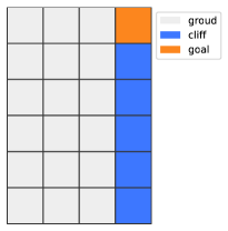
Figure 1: Layout of the gridworld

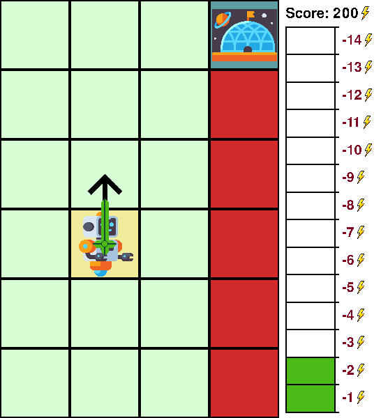
Figure 2: Layout of the game

Unsurprisingly, when a human plays the game, they do not not follow the exact optimal policy. This is problematic as the simple IRL agent above assumes that the optimal policy is known and deterministic. To resolve this issue, we developed another method which we call the loss IRL agent,

$$\mathcal{L}(R_{S})=\sum_{s\in S}\exp\left(\operatorname{ReLU}\left(\sum_{a\in A}\pi(s,a)\max_{a^{\prime}\in A\backslash\{a\}}Q(s,a^{\prime})-Q(s,a)\right)\right)$$ (3)

We will minimise the loss, $\mathcal{L}(R_{S})$. We would expect that $Q$ would be highest for the action most preferred by the policy. When the most preferred action for a given state results in the largest $Q$ value, the term inside the $\operatorname{ReLU}$ will be 0, otherwise, it will be positive.

4 Experimental results

MaxEnt baselines As a baseline, we use a MaxEnt method without carefulness from Kim et al. (2021). We choose this method because it is guaranteed to recover the reward in the limit of infinite data, even without carefulness. The method has deterministic transitions with policy

$$\pi(a|s) =\frac{1}{Z(s)}e^{\beta Q(s,a)}$$ (4)

where $\beta$ is a hyperparameter and $Z(s)$ ensures that the distribution over actions normalizes to $1$. Kim et al. (2021) guarantees the existence of a unique optimal reward function for this setting. We generated 10000 rollouts from an agent in this environment and recover a reward function which is shown in Figure 5. Thus, while this reward function accurately captures the existence of both the cliff and the goal state, it massively underestimates the severity of the penalty for falling off the cliff, and this likely indicates the need for far more samples to accurately estimate the rewards.

Simple IRL agent. This is for the agent described in Section 3. We solve the MDP using value-iteration to get an optimal policy for the setting with 14 levels of carefulness. The policy is shown in Figure 3. As we would expect, the optimal actions when closer to the cliff are to be more careful and often to move away from the cliff.

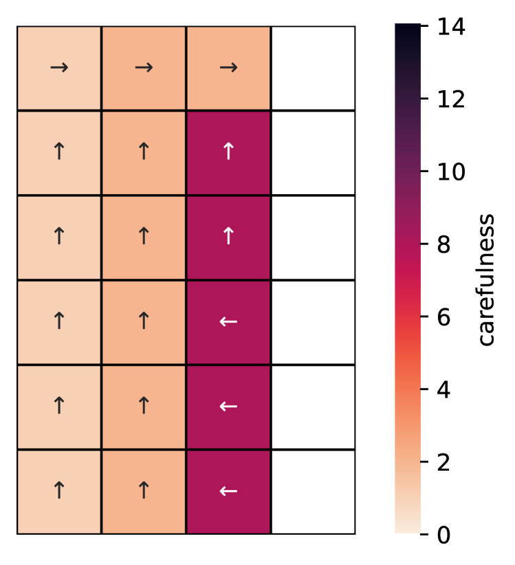
Figure 3: Optimal policy for the setting with 14 levels of carefulness

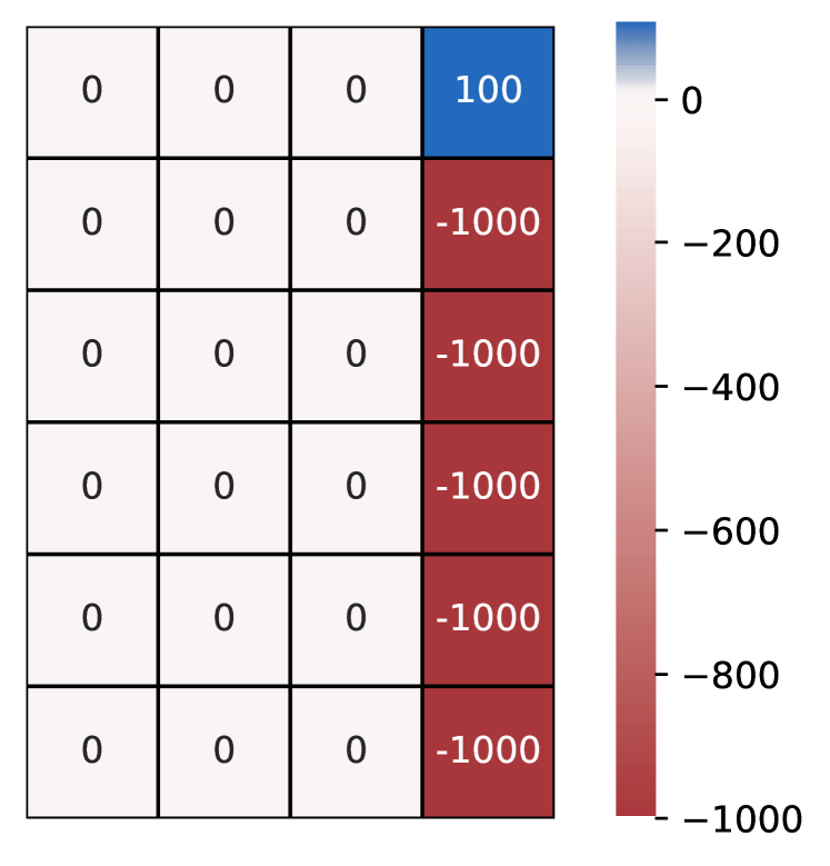
Figure 4: True reward

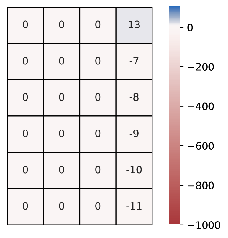
Figure 5: Learned reward using computer generated rollouts in the benchmark setting

We generated 100 rollouts with the agent starting in a random “ground” state (see Figure 1) and then following the optimal policy shown in Figure 3. We then use these rollouts to train the simple IRL agent using a maximum reward of 1000 and we used $\lambda=0$. By leveraging carefulness, we are able to learn the severity of the reward function; see Figure 6.

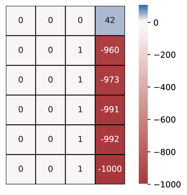
Figure 6: Learned reward using computer generated rollouts

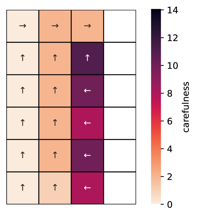
Figure 7: Policy followed by the human

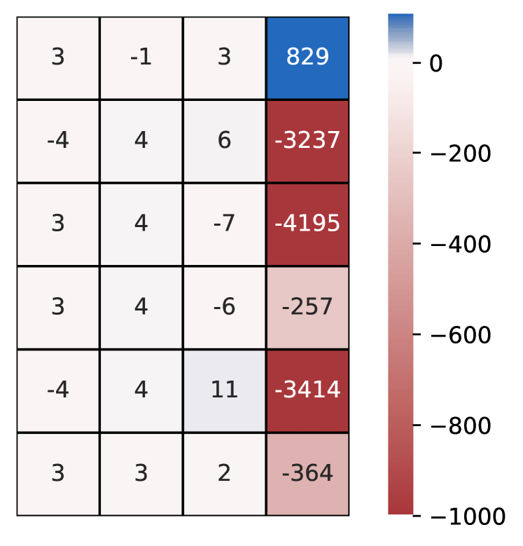
Figure 8: Learned reward from human rollouts

Loss IRL agent. An expert human (one of the authors) played the game for 10 rollouts (vs 10,000 optimal rollouts for the baseline). Note that some states will have been visited on multiple occasions and that different actions may have been selected on each visitation and so the policy is not deterministic. The most commonly chosen action for each state is shown in Figure 8. An agent as described in Section 3 was trained on the rollouts and the reward obtained is shown in Figure 8; compare to the true reward in Figure 4 and the benchmark reward in Figure 5. While there is considerable variability in the inferred rewards, likely due to only having 10 rollouts, we have achieved our aim, which was to capture the severity of the penalty for falling off the cliff.

5 Conclusion and future work

We have shown that IRL can distinguish between catastrophic and merely undesirable rewards if it takes account of human carefulness. We validated this idea on a simple gridworld task where the human explicitly inputs a degree of carefulness. In future work, it will be important to extend these ideas to more complex settings (such as robotic simulators) and to understand how to infer carefulness from actual human actions (e.g. by using the speed of actions as a proxy).

Appendix A Background

A (finite) Markov decision process (MDP) is defined as the tuple $(S,A,T,\gamma,R)$ where

• $S$ is a finite set of $N_{S}$ states

• $A$ is a finite set of $N_{A}$ actions

• $T(s,a,s^{\prime})$ is the probability of transitioning from state $s$ to state $s^{\prime}$ when undertaking action $a$

• $\gamma\in[0,1)$ is the discount factor

• $R(s,a)$ is the reward received from transitioning out of state $s$ via action $a$

A policy is defined as a function $\pi:S\times A\rightarrow[0,1]$. A value function for a given policy is a map $V^{\pi}:S\rightarrow\mathbb{R}$ and represents the expected discounted reward when following policy $\pi$ from a given state. It is recursively given by

$$V^{\pi}(s)=\sum_{a\in A}\pi(s,a)\left(R(s,a)+\gamma\sum_{s^{\prime}\in S}T(s,a,s^{\prime})V^{\pi}(s^{\prime})\right)$$ (5)

A related quantity is the action-value function, $Q^{\pi}:S\times A\rightarrow\mathbb{R}$. $Q^{\pi}(s,a)$ is the expected discounted reward when starting from state $s$, immediately following action $a$ and then following policy $\pi$. It is given in terms of $V^{\pi}$ by

$$Q^{\pi}(s,a)=R(s,a)+\gamma\sum_{s^{\prime}\in S}T(s,a,s^{\prime})V^{\pi}(s^{\prime})$$

Appendix B Proofs for IRL agent

Theorem 1.

$$\bm{V}^{\pi}=(\bm{I}_{N_{S}}-\gamma\bm{T}^{\pi})^{-1}\hat{\bm{\pi}}\operatorname{vec}(\bm{R})$$

Where $N_{S}:=|S|$, $\bm{T}^{\pi}$ is the $N_{S}$ by $N_{S}$ matrix giving the probability of transitioning from one state to another when following the optimal policy, and $\hat{\bm{\pi}}$ is the $N_{S}$ by $N_{S}N_{A}$ matrix such that $\hat{\bm{\pi}}\operatorname{vec}(\bm{R})=\bm{R}^{\pi}$ and $\bm{R}^{\pi}$ is the expected immediate reward for transitioning whilst following $\pi$.

Proof.

We have that, $\forall s\in S$

$$V^{\pi}(s) =\sum_{a\in A}\pi(s,a)\left(R(s,a)+\gamma\sum_{s^{\prime}\in S}T(s,a,s^{\prime})V^{\pi}(s^{\prime})\right)$$

$$V^{\pi}(s) =\sum_{a\in A}\pi(s,a)\left(\bm{R}_{s,a}+\gamma\bm{T}_{s,a}\bm{V}^{\pi}\right)$$

and so

$$\bm{V}^{\pi} =\bm{R}^{\pi}+\gamma\bm{T}^{\pi}\bm{V}^{\pi}$$

$$(\bm{I}-\gamma\bm{T}^{\pi})\bm{V}^{\pi} =\bm{R}^{\pi}$$

$$\bm{V}^{\pi} =(\bm{I}-\gamma\bm{T}^{\pi})^{-1}\hat{\bm{\pi}}\operatorname{vec}{\bm{R}}$$

∎

Theorem 2.

$$\bm{Q}^{\pi}=\left(\hat{\bm{I}}+\gamma\bm{T}(\bm{I}_{N_{S}}-\gamma\bm{T}^{\pi})^{-1}\hat{\bm{\pi}}\right)\operatorname{vec}(\bm{R})$$

where $\hat{\bm{I}}$ is $\bm{I}_{N_{S}N_{A}}$ reshaped to be $N_{S}$ by $N_{A}$ by $N_{S}N_{A}$

Proof.

$$Q^{\pi}(s,a) =R(s,a)+\gamma\sum_{s^{\prime}\in S}\bm{T}_{s,a}(s^{\prime})V^{\pi}(s^{\prime})$$

$$\bm{Q}^{\pi} =\bm{R}+\gamma\bm{T}\bm{V}^{\pi}$$

$$\bm{Q}^{\pi} =\bm{R}+\gamma\bm{T}(\bm{I}_{N_{S}}-\gamma\bm{T}^{\pi})^{-1}\hat{\bm{\pi}}\operatorname{vec}({\bm{R}})$$

$$\bm{Q}^{\pi} =\left(\hat{\bm{I}}+\gamma\bm{T}(\bm{I}_{N_{S}}-\gamma\bm{T}^{\pi})^{-1}\bm{\hat{\pi}}\right)\operatorname{vec}{(\bm{R})}$$

∎

Theorem 3.

For a reward function $\bm{R}$ to be valid, we require that

$$\left\{\left[\widetilde{\bm{I}}_{N_{S}}+\gamma(\widetilde{\bm{T}}^{\pi}-\bm{T})(\bm{I}_{N_{S}}-\gamma\bm{T}^{\pi})^{-1}\right]\hat{\bm{\pi}}-\hat{\bm{I}}\right\}\operatorname{vec}(\bm{R})\succeq 0$$

where

• For a matrix $\bm{X}$ of dimension $N_{S}$ by $N_{S}$, $\widetilde{\bm{X}}$ is the matrix obtained by stacking $N_{A}$ copies of $\bm{X}$ giving a matrix of dimension $N_{S}$ by $N_{A}$ by $N_{S}$

• For matrices $\bm{X}$ of dimension $n$ by $m$, and $c\in\mathbb{R}$, $\bm{X}\succeq c$ means that for all $0\leq i\leq n$ and $0\leq j\leq m$, $\bm{X}_{i,j}\geq c$

Proof.

The policy $\pi$ is optimal if and only if $\forall s\in S$ and $\forall a\in A$

$$Q^{\pi}(s,\pi(s))\geq Q^{\pi}(s,a^{\prime})$$

$$\qquad\Leftrightarrow\bm{R}_{s,\pi(s)}+\gamma\left(\bm{T}^{\pi}\bm{V}^{\pi}\right)_{s}\geq\bm{R}_{s,a}+\gamma\left(\bm{T}_{:,a,:}\bm{V}^{\pi}\right)_{s}$$

$$\qquad\Leftrightarrow\bm{R}^{\pi}+\gamma\bm{T}^{\pi}\bm{V}^{\pi}\succeq\bm{R}_{:,a}+\gamma\bm{T}_{:,a,:}\bm{V}^{\pi}$$

$$\qquad\Leftrightarrow\hat{\bm{\pi}}\operatorname{vec}{(\bm{R})}-\bm{R}_{:,a}\succeq\gamma(\bm{T}_{:,a,:}\bm{V}^{\pi}-\bm{T}^{\pi}\bm{V}^{\pi})$$

$$\qquad\Leftrightarrow\hat{\bm{\pi}}\operatorname{vec}{(\bm{R})}-\bm{R}_{:,a}\succeq\gamma(\bm{T}_{:,a,:}-\bm{T}^{\pi})\bm{V}^{\pi}$$

$$\qquad\Leftrightarrow\hat{\bm{\pi}}\operatorname{vec}{(\bm{R})}-\bm{R}_{:,a}\succeq\gamma(\bm{T}_{:,a,:}-\bm{T}^{\pi})(\bm{I}_{N_{S}}-\gamma\bm{T}^{\pi})^{-1}\hat{\bm{\pi}}\operatorname{vec}(\bm{R})$$

$$\qquad\Leftrightarrow\hat{\bm{\pi}}\operatorname{vec}(\bm{R})-\gamma(\bm{T}_{:,a,:}-\bm{T}^{\pi})(\bm{I}_{N_{S}}-\gamma\bm{T}^{\pi})^{-1}\hat{\bm{\pi}}\operatorname{vec}(\bm{R})-\bm{R}_{:,a}\succeq 0$$

$$\qquad\Leftrightarrow\left[\bm{I}_{N_{S}}+\gamma(\bm{T}^{\pi}-\bm{T}_{:,a,:})(\bm{I}_{N_{S}}-\gamma\bm{T}^{\pi})^{-1}\right]\hat{\bm{\pi}}\operatorname{vec}(\bm{R})-\bm{R}_{:,a}\succeq 0$$

$$\qquad\Leftrightarrow\left[\widetilde{\bm{I}}_{N_{S}}+\gamma(\widetilde{\bm{T}}^{\pi}-\bm{T})(\bm{I}_{N_{S}}-\gamma\bm{T}^{\pi})^{-1}\right]\hat{\bm{\pi}}\operatorname{vec}(\bm{R})-\bm{R}\succeq 0$$

∎

Theorem 4.

Maximising expression (1) is equivalent to minimising

$$\sum_{s\in S}\max_{a\in A\backslash\{\pi(s)\}}\left(\hat{\bm{I}}-\left(\widetilde{\bm{I}}_{N_{S}}-\gamma\bm{T}\right)\left(\bm{I}_{N_{S}}-\gamma\bm{T}^{\pi}\right)^{-1}\hat{\bm{\pi}}\right)_{s,a}\cdot\operatorname{vec}(\bm{R})+\lambda||\bm{R}||_{1}$$ (6)

Proof.

Maximising expression (1) is equivalent to minimising

$$\sum_{s\in S}\left\{\max_{a\in A\backslash\{\pi(s)\}}\left(\bm{Q}^{\pi}_{s,a}\right)-\bm{Q}^{\pi}_{s,\pi(s)}\right\}+\lambda||\bm{R}||_{1}$$

$$\qquad=\sum_{s\in S}\max_{a\in A\backslash\{\pi(s)\}}\left(\bm{Q}^{\pi}_{s,a}-\bm{V}^{\pi}_{s}\right)+\lambda||\bm{R}||_{1}$$

$$\qquad=\sum_{s\in S}\max_{a\in A\backslash\{\pi(s)\}}\left(\bm{Q}^{\pi}-\widetilde{\bm{I}}_{N_{S}}\bm{V}\right)_{s,a}+\lambda||\bm{R}||_{1}$$

$$\qquad=\sum_{s\in S}\max_{a\in A\backslash\{\pi(s)\}}\left\{\left(\hat{\bm{I}}-\left(\widetilde{\bm{I}}_{N_{S}}-\gamma\bm{T}\right)\left(\bm{I}_{N_{S}}-\gamma\bm{T}^{\pi}\right)^{-1}\hat{\bm{\pi}}\right)_{s,a}\cdot\operatorname{vec}(\bm{R})\right\}$$

$$\qquad\qquad+\lambda||\bm{R}||_{1}$$

∎

In the tabular setting, we can express Equation 2 as

$$\operatorname{vec}(\bm{R})=\operatorname{vec}(\bm{R}_{A})+\hat{\mathbb{1}}_{N_{s},N_{A}}^{\intercal}\bm{R}_{S}$$

Where $\hat{\mathbb{1}}_{N_{s},N_{A}}^{\intercal}$ is such that $\hat{\mathbb{1}}_{N_{s},N_{A}}^{\intercal}\bm{R}_{S}$ equal to $N_{A}$ copies of $\bm{R}_{S}$ stacked on top of each other.

Theorem 5.

Writing $\bm{\Omega}=\hat{\bm{I}}-\left(\widetilde{\bm{I}}_{N_{S}}-\gamma\bm{T}\right)\left(\bm{I}_{N_{S}}-\gamma\bm{T}^{\pi}\right)^{-1}\hat{\bm{\pi}}$, minimising expression (6) is equivalent to minimising

$$\sum_{s\in S}\max_{a\in A\backslash\{\pi(s)\}}\bm{\Omega}_{s,a}\hat{\mathbb{1}}_{N_{s},N_{A}}^{\intercal}\bm{R}_{S}+\lambda\left|\left|\bm{R}_{S}\right|\right|_{1}$$ (7)

Proof.

Expression (6) is

$$\sum_{s\in S}\max_{a\in A\backslash\{\pi(s)\}}\bm{\Omega}_{s,a}\operatorname{vec}(\bm{R})+\lambda||\bm{R}||_{1}$$

$$\qquad=\sum_{s\in S}\max_{a\in A\backslash\{\pi(s)\}}\bm{\Omega}_{s,a}\left(\operatorname{vec}(\bm{R}_{A})+\hat{\mathbb{1}}_{N_{s},N_{A}}^{\intercal}\bm{R}_{S}\right)$$

$$\qquad\qquad+\lambda\left|\left|\operatorname{vec}(\bm{R}_{A})+\hat{\mathbb{1}}_{N_{s},N_{A}}^{\intercal}\bm{R}_{S}\right|\right|_{1}$$

As the second term is an arbitrary choice to encourage more zeros in the reward, we can replace it with $||\bm{R}_{S}||_{1}$. We therefore get that we want to minimise

$$\sum_{s}\left\{\max_{a\in A\backslash\{\pi(s)\}}\left(\bm{\Omega}_{s,a}\operatorname{vec}(\bm{R}_{A})\right)+\max_{a\in A\backslash\{\pi(s)\}}\left(\bm{\Omega}_{s,a}\hat{\mathbb{1}}_{N_{s},N_{A}}^{\intercal}\bm{R}_{S}\right)\right\}+\lambda||\bm{R}_{S}||_{1}$$

And since $\bm{R}_{A}$ is fixed, we get

$$\sum_{s\in S}\max_{a\in A\backslash\{\pi(s)\}}\bm{\Omega}_{s,a}\hat{\mathbb{1}}_{N_{s},N_{A}}^{\intercal}\bm{R}_{S}+\lambda\left|\left|\bm{R}_{S}\right|\right|_{1}$$

∎

References

- Achiam et al. (2017) Joshua Achiam, David Held, Aviv Tamar, and Pieter Abbeel. Constrained policy optimization. In Doina Precup and Yee Whye Teh (eds.), Proceedings of the 34th International Conference on Machine Learning, volume 70 of Proceedings of Machine Learning Research, pp. 22–31. PMLR, 06–11 Aug 2017. URL https://proceedings.mlr.press/v70/achiam17a.html.
- Alshiekh et al. (2018) Mohammed Alshiekh, Roderick Bloem, Rüdiger Ehlers, Bettina Könighofer, Scott Niekum, and Ufuk Topcu. Safe reinforcement learning via shielding. In Proceedings of the AAAI Conference on Artificial Intelligence, volume 32, 2018.
- Anderson et al. (2022) Martin Anderson, Lieven Vandenberghe, and Joachim Dahl. CVXOPT, 2022. URL https://cvxopt.org.
- Askew & Field (2008) Chris Askew and Andy P Field. The vicarious learning pathway to fear 40 years on. Clinical psychology review, 28(7):1249–1265, 2008.
- Berkenkamp et al. (2017) Felix Berkenkamp, Matteo Turchetta, Angela Schoellig, and Andreas Krause. Safe model-based reinforcement learning with stability guarantees. In I. Guyon, U. Von Luxburg, S. Bengio, H. Wallach, R. Fergus, S. Vishwanathan, and R. Garnett (eds.), Advances in Neural Information Processing Systems, volume 30. Curran Associates, Inc., 2017. URL https://proceedings.neurips.cc/paper/2017/file/766ebcd59621e305170616ba3d3dac32-Paper.pdf.
- Brown & Niekum (2018) Daniel Brown and Scott Niekum. Efficient probabilistic performance bounds for inverse reinforcement learning. Proceedings of the AAAI Conference on Artificial Intelligence, 32(1), Apr. 2018. doi: 10.1609/aaai.v32i1.11755. URL https://ojs.aaai.org/index.php/AAAI/article/view/11755.
- Brown et al. (2018) Daniel S. Brown, Yuchen Cui, and Scott Niekum. Risk-aware active inverse reinforcement learning. In Aude Billard, Anca Dragan, Jan Peters, and Jun Morimoto (eds.), Proceedings of The 2nd Conference on Robot Learning, volume 87 of Proceedings of Machine Learning Research, pp. 362–372. PMLR, 29–31 Oct 2018. URL https://proceedings.mlr.press/v87/brown18a.html.
- Dunne & Askew (2013) Guler Dunne and Chris Askew. Vicarious learning and unlearning of fear in childhood via mother and stranger models. Emotion, 13(5):974, 2013.
- Finn et al. (2016) Chelsea Finn, Sergey Levine, and Pieter Abbeel. Guided cost learning: Deep inverse optimal control via policy optimization. In International Conference on Machine Learning, pp. 49–58. PMLR, Jun 2016. URL https://proceedings.mlr.press/v48/finn16.html.
- Galin et al. (2020) Rinat Galin, Roman Meshcheryakov, Saniya Kamesheva, and Anna Samoshina. Cobots and the benefits of their implementation in intelligent manufacturing. In IOP conference series: Materials science and engineering, volume 862, pp. 032075. IOP Publishing, 2020.
- Garcia & Fernández (2012) Javier Garcia and Fernando Fernández. Safe exploration of state and action spaces in reinforcement learning. Journal of Artificial Intelligence Research, 45:515–564, 2012.
- Henley (2022) Jon Henley. Chess robot grabs and breaks finger of seven-year-old opponent. The Guardian, 2022. URL https://www.theguardian.com/sport/2022/jul/24/chess-robot-grabs-and-breaks-finger-of-seven-year-old-opponent-moscow.
- Hjorth & Chrysostomou (2022) Sebastian Hjorth and Dimitrios Chrysostomou. Human–robot collaboration in industrial environments: A literature review on non-destructive disassembly. Robotics and Computer-Integrated Manufacturing, 73:102208, 2022.
- Ho & Ermon (2016) Jonathan Ho and Stefano Ermon. Generative adversarial imitation learning. In Advances in Neural Information Processing Systems, volume 29. Curran Associates, Inc., 2016. URL https://papers.nips.cc/paper/2016/hash/cc7e2b878868cbae992d1fb743995d8f-Abstract.html.
- Kim et al. (2021) Kuno Kim, Shivam Garg, Kirankumar Shiragur, and Stefano Ermon. Reward identification in inverse reinforcement learning. In Marina Meila and Tong Zhang (eds.), Proceedings of the 38th International Conference on Machine Learning, volume 139 of Proceedings of Machine Learning Research, pp. 5496–5505. PMLR, 18–24 Jul 2021. URL https://proceedings.mlr.press/v139/kim21c.html.
- Marin et al. (2020) Marie-France Marin, Alexe Bilodeau-Houle, Simon Morand-Beaulieu, Alexandra Brouillard, Ryan J Herringa, and Mohammed R Milad. Vicarious conditioned fear acquisition and extinction in child–parent dyads. Scientific reports, 10(1):1–10, 2020.
- Menda et al. (2017) Kunal Menda, Katherine Driggs-Campbell, and Mykel J Kochenderfer. Dropoutdagger: A bayesian approach to safe imitation learning. arXiv preprint arXiv:1709.06166, 2017.
- Menda et al. (2019) Kunal Menda, Katherine Driggs-Campbell, and Mykel J Kochenderfer. Ensembledagger: A bayesian approach to safe imitation learning. In 2019 IEEE/RSJ International Conference on Intelligent Robots and Systems (IROS), pp. 5041–5048. IEEE, 2019.
- Michalos et al. (2022) George Michalos, Panagiotis Karagiannis, Nikos Dimitropoulos, Dionisis Andronas, and Sotiris Makris. Human robot collaboration in industrial environments. In The 21st Century Industrial Robot: When Tools Become Collaborators, pp. 17–39. Springer, 2022.
- Mineka & Cook (1993) Susan Mineka and Michael Cook. Mechanisms involved in the observational conditioning of fear. Journal of Experimental Psychology: General, 122(1):23, 1993.
- Moreno et al. (2020) Miguel Ángel Moreno, Diego Carou, and J Paulo Davim. Autonomous robots and cobots: Applications in manufacturing. In Enabling Technologies for the Successful Deployment of Industry 4.0, pp. 47–66. CRC Press, 2020.
- Ng & Russell (2000) Andrew Y Ng and Stuart J Russell. Algorithms for inverse reinforcement learning. In ICML, 2000.
- Paine et al. (2018) Tom Le Paine, Sergio Gómez Colmenarejo, Ziyu Wang, Scott Reed, Yusuf Aytar, Tobias Pfaff, Matt W Hoffman, Gabriel Barth-Maron, Serkan Cabi, David Budden, et al. One-shot high-fidelity imitation: Training large-scale deep nets with rl. arXiv preprint arXiv:1810.05017, 2018.
- Peng et al. (2018a) Xue Bin Peng, Pieter Abbeel, Sergey Levine, and Michiel van de Panne. Deepmimic: example-guided deep reinforcement learning of physics-based character skills. ACM Transactions on Graphics, 37(4):1–14, Aug 2018a. ISSN 0730-0301, 1557-7368. doi: 10.1145/3197517.3201311.
- Peng et al. (2018b) Xue Bin Peng, Angjoo Kanazawa, Sam Toyer, Pieter Abbeel, and Sergey Levine. Variational discriminator bottleneck: Improving imitation learning, inverse rl, and gans by constraining information flow. arXiv preprint arXiv:1810.00821, 2018b.
- Ramachandran & Amir (2007) Deepak Ramachandran and Eyal Amir. Bayesian inverse reinforcement learning. In IJCAI, volume 7, pp. 2586–2591, 2007.
- Reynolds et al. (2018) Gemma Reynolds, Andy P Field, and Chris Askew. Reductions in children’s vicariously learnt avoidance and heart rate responses using positive modeling. Journal of Clinical Child & Adolescent Psychology, 47(4):555–568, 2018.
- Russell (1998) Stuart Russell. Learning agents for uncertain environments (extended abstract). In Proceedings of the eleventh annual conference on Computational learning theory - COLT’ 98, pp. 101–103, Madison, Wisconsin, United States, 1998. ACM Press. ISBN 978-1-58113-057-7. doi: 10.1145/279943.279964. URL http://portal.acm.org/citation.cfm?doid=279943.279964.
- Saunders et al. (2017) William Saunders, Girish Sastry, Andreas Stuhlmueller, and Owain Evans. Trial without error: Towards safe reinforcement learning via human intervention. arXiv preprint arXiv:1707.05173, 2017.
- Simoes et al. (2019) Ana C Simoes, António Lucas Soares, and Ana C Barros. Drivers impacting cobots adoption in manufacturing context: A qualitative study. In International Scientific-Technical Conference MANUFACTURING, pp. 203–212. Springer, 2019.
- Sutton & Barto (2018) Richard S Sutton and Andrew G Barto. Reinforcement learning: An introduction. MIT press, 2018.
- Ziebart et al. (2008) Brian D Ziebart, Andrew L Maas, J Andrew Bagnell, Anind K Dey, et al. Maximum entropy inverse reinforcement learning. In AAAI, volume 8, pp. 1433–1438. Chicago, IL, USA, 2008.