OGLE-2016-BLG-1195Lb: A sub-Neptune Beyond the Snow Line of an M-dwarf Confirmed by Keck AO

Abstract

We present the analysis of high resolution follow-up observations of OGLE-2016-BLG-1195 using Keck, four years after the event’s peak. We find the lens system to be at $D_{L}=6.87\pm 0.65$ kpc and comprised of a $M_{\rm p}=9.91\pm 1.61\ M_{\rm Earth}$ planet, orbiting an M-dwarf, $M_{\rm L}=0.57\pm 0.06\ M_{\odot}$, beyond the snow line, with a projected separation of $r_{\perp}=2.62\pm 0.28$ AU. Our results are consistent with the discovery paper, which reports values with 1-sigma uncertainties based on a single mass-distance constraint from finite source effects. However, both the discovery paper and our follow-up results disagree with the analysis of a different group that also present the planetary signal detection. The latter utilizes Spitzer photometry to measure a parallax signal. Combined with finite source effects, they claim to measure the mass and distance of the system to much greater accuracy, suggesting that it is composed of an Earth-mass planet orbiting an ultracool dwarf. Their parallax signal though is improbable since it suggests a lens star in the disk moving perpendicular to disk rotation. Moreover, parallaxes are known to be affected by systematic errors in the photometry. Therefore, we reanalyze the Spitzer photometry for this event and conclude that the parallax signal is not significantly greater than the instrumental noise, and is likely affected by systematic errors in the photometric data. The results of this paper act as a cautionary tale that conclusions of analyses that rely heavily on low signal-to-noise Spitzer photometric data, can be misleading.

tablenum SIXtablenum

1 Introduction

Gravitational microlensing is a unique method that can detect Earth to super-Jupiter mass exoplanets in wide orbits beyond the snow line (Bennett & Rhie, 1996; Mao & Paczynski, 1991; Gould & Loeb, 1992). The snow line refers to a region just beyond the habitable zone where water can only be sustained in the form of ice, and it is the predicted region where more massive planets form (Lissauer, 1993; Ida & Lin, 2004; Kennedy et al., 2006). Statistical studies have shown that the frequency of planets beyond the snow line (especially ice and gas giants), is about 7 times greater than smaller separation systems (Gould et al., 2010; Cumming et al., 2008).

Contrary to other planetary detection techniques, microlensing can detect planets without using any light from the host star. This allows for a range of stellar type hosts to be probed, e.g. Solar-type, M dwarfs and white dwarfs (Blackman et al., 2021). In addition, this method can investigate more distant planetary systems in our galaxy towards the Galactic Bulge, thus complementing the other detection techniques that typically probe the Solar neighborhood.

The advantages of microlensing, however, also bring certain caveats. Not directly detecting the light from the host star means that the physical parameters of the system, such as mass and distance, cannot be determined easily. Instead, the method accurately constrains the host-planet mass ratio, which although a fundamental property, is not as informative as a mass-measurement to the wider exoplanet community. The individual masses of a planetary microlensing event can be determined if both second-order effects on the light curve are measured; finite source effects (features due to the source radius) and the microlensing parallax, $\pi_{E}$. Most planetary microlensing events exhibit finite source effects, however, observable parallax effects are uncommon. Using just the finite source effects, the physical parameters can be estimated using a Bayesian analysis with a Galactic model as a prior (Beaulieu et al., 2006; Gaudi et al., 2008). However, this method typically yields poorly constrained parameters, since it only uses a single constraint. Parameters can be estimated with greater precision when additional constraints on the mass-distance relation are added.

A complementary mass-measurement method that has been successful, is high angular resolution follow-up observations from 8-10m class ground telescopes, or the Hubble Space Telescope. Follow-up observations can take place several years after the microlensing event has occurred, which means the source and lens can be resolved and their fluxes measured individually (e.g. Bhattacharya et al. (2018); Vandorou et al. (2020); Terry et al. (2021)). With this method it is also important to identify the lens star, since companions to either the lens and source, can also be mistaken for the lens system. The source star can be identified by comparing the candidate lens-source separations to the relative proper motion predicted by the light curve model.

In this paper we present the Keck follow-up observations of OGLE-2016-BLG-1195 (henceforth, OB161195) used to resolve the source and lens. We measure their flux ratio and separation, and constrain the relative source-lens proper motion, thus obtaining accurate physical properties of the planetary system.

2 Microlensing Event OGLE-2016-BLG-1195

The microlensing event OB161195 was alerted by the Optical Gravitational Lens Experiment (OGLE, Udalski et al. (1994), Udalski (2003)) on June 27 2016. The event was also independently alerted by the Microlensing Observations in Astrophysics (MOA, Bond et al. (2001)) collaboration on June 28 2016, where a 2.5 hour photometric perturbation was discovered (the event has the alternative name of MOA-2016-BLG-350). Observations were taken in the I and V band with OGLE, and R and V band with MOA. OB161195 is located towards the Galactic Bulge at (RA, Dec) = (17:55:23.50, -30:12:26.1).

The data, modeling and analyses of the microlensing light curve is presented in Bond et al. (2017) (henceforth, B17). The event exhibits a planetary anomaly with a mass-ratio, $q=4.2\pm 0.7\times 10^{-5}$, which at the time of detection was the lowest mass-ratio found in microlensing. The Einstein ring radius ($\theta_{E}$) was derived from the microlensing parameters (Einstein radius crossing time, $t_{E}$, and the source radius crossing time, $t_{*}$) and the angular size measurement of the source star, $\theta_{s}$. The physical parameters of the lensing system were estimated by employing a Bayesian technique, as described in Bennett et al. (2008). A Galactic model was used which comprised of a double-exponential disk (Reid et al., 2002) and a bar model (Han & Gould, 1995). The Bayesian estimate of the lens mass was found to be $M_{L}=0.37^{+0.38}_{-0.21}\ M_{\odot}$, at a distance of $D_{L}=7.20^{+0.80}_{-1.02}$ kpc. These values imply a planet mass of approximately $M_{\rm planet}=5.10^{+5.5}_{-2.85}\ M_{\rm Earth}$. The high uncertainties of these values are due to there only being a single mass-distance constraint, the $\theta_{E}$ value, therefore the Bayesian result is highly dependent on the prior assumption that stars of all masses are equally likely to host a plant.

In parallel, the event was also observed in the paw-print of the Korean Microlensing Telescope Network (KMTNet, Kim et al. (2016)), which operates three 1.6m telescopes equipped with 4 square degree wide field imagers. Their data were taken in survey mode with the majority in I band, and only a few in V, and it was not influenced by the OGLE and MOA alert. Their data confirmed a planetary perturbation in the light curve which was presented in Shvartzvald et al. (2017) (henceforth, S17). Their source star characteristics, extinction determination, mass-ratio and projected separations from the light curve model are in agreement with B17. The light curve parameters from both detection papers can be found in Table 1.

Subsequent Spitzer observations were also obtained with a cadence of one observation per day. A strong microlens parallax of $\pi_{E}\sim$ 0.45 was retrieved by fitting the KMTNet and Spitzer light curves simultaneously, however, the low signal-to-noise Spitzer data (presented in Figure 1 of S17) is seen to systematically differ from the model. In addition, S17 report a lens-source relative proper motion of $\mu_{\rm hel}(N,E)\equiv(\pm 4.0,-7.5)$ mas/yr measured from their parallax value, which suggests a counter-rotating lens in the disk.

Combining this Spitzer parallax with the light curve model parameters from the KMTNet observations, S17 found the system to be an Earth-mass planet, $M_{\rm planet}=1.43^{+0.45}_{-0.32}M_{\rm Earth}$, orbiting an ultra-cool dwarf, $M_{L}=0.078^{+0.016}_{-0.012}M_{\odot}$, at a distance of $D=3.19^{+0.42}_{-0.46}$ kpc. The large difference between the conclusions of B17 and S17 are entirely due to the Spitzer data and their constraint on the parallax measurement. This measurement, and the reason for the discrepancy, is investigated in Section 5.1.

Table 1: Light curve model parameters from Bond et al. (2017) and Shvartzvald et al. (2017). The table shows the Einstein radius crossing time, $t_{E}$; the impact parameter, $u_{0}$; instantaneous projected separation (scaled to $\theta_{E}$), $s$; the ratio of the angular size of the companion to that of the Einstein ring and the coefficient,$\rho$; the mass ratio, $q$; and the Einstein angular ring radius, $\theta_{E}$.

Parameters	Bond17	Shvartzvald17
$t_{E}$ (days)	10.16$\pm$ 0.25	9.96 $\pm$ 0.11
$u_{0}$	0.0514 $\pm$ 0.0014	0.0532 $\pm$ 0.0007
s	1.0698 $\pm$ 0.0078	$1.0348^{+0.0080}_{-0.0075}$
$\rho$	0.00328 $\pm$ 0.00026	$0.00287^{+0.34}_{-0.38}$
$q/10^{-5}$	4.25 $\pm$ 0.67	$5.55^{+0.84}_{-0.71}$
$\theta_{E}$ (mas)	0.261 $\pm$ 0.020	$0.286^{+0.053}_{-0.038}$

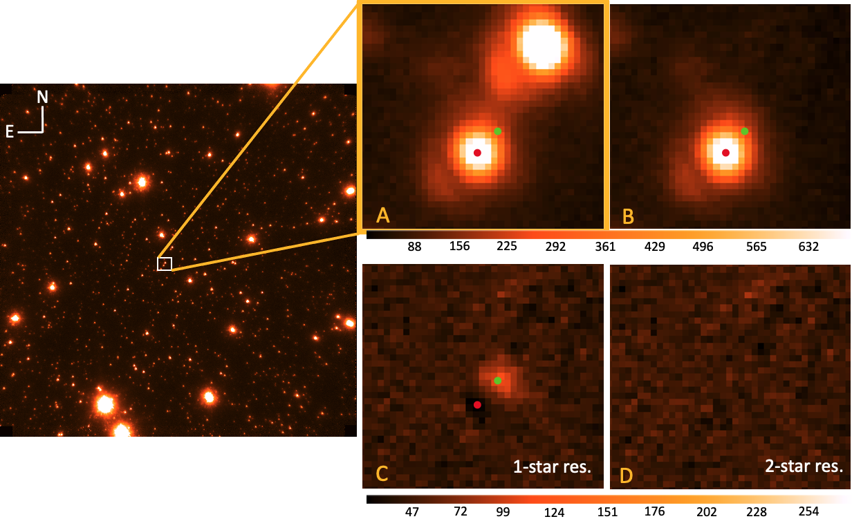
Figure 1: Keck Osiris image from the 2020 observing run using the narrow camera with a pixel size of $\sim$0.01 arcseconds/pixel, in K-band. Panel A marks the target as the red dot and the position of the residual with a green dot. Panel B shows the target after a nearby bright star, North West of the target, is subtracted. Panel C shows the residuals from a 1-star fit using DAOPHOT, and panel D shows the smooth residuals from a 2-star fit.

3 Keck Follow-up of OGLE-2016-BLG-1195

We observed OB161195 with Keck II’s NIRC2 AO system on August 3 2018. We used the wide camera with a plate scale of 0.04 arcseconds/pixel. Images were taken using the $K_{\rm short}$ (henceforth, $K$) passband, where 15 good images were obtained. The exposure time of the images was 30 seconds with a dither of $\sim 2^{\prime\prime}$. We reduced the images using the standard techniques described in Beaulieu et al. (2016) and Batista et al. (2014). This procedure includes dark current and flat-field correction. After sky correcting the wide-frame images, they were stacked using SWARP (Bertin, 2010) and the stellar fluxes were measured using aperture photometry with SExtractor (Bertin & Arnouts, 1996). We cross identify 71 stars in our stacked wide-frame with VVV survey data (Minniti et al., 2010) as described in Beaulieu (2018). This allowed us to calibrate our K band Keck photometry. Thus, the total measured combined K band magnitude of both source and lens is:

$$K_{\rm Keck}=16.92\pm 0.02.$$

On August 9 2020, OB161195 was observed with Keck’s Osiris instrument. Osiris has a camera with plate scale of 0.01 arcseconds/pixel. 14 usable images were obtained in $\rm K_{prime}$ (hereafter, $\rm K_{p}$) band and reduced using the KAI pipeline (Lu et al., 2021). The quality of these images were good, with a FWHM (full-width-half-maximum) of $\sim 60$ mas across the frame. The predicted separation between the source and lens is estimated to be about 39 mas in 2020 ($\sim 4.12$ years after peak magnification) with a predicted source-lens relative proper motion of $\mu_{\rm rel}=9.38\pm 0.75$ $\rm mas/yr^{-1}$ (Bond et al., 2017). Since this separation is less than 1 FWHM we found it necessary to use point spread function (PSF) fitting photometry routine to see if we can indeed resolve the source and lens. For a more robust result we used two methods, one using the standard DAOPHOT routine (Bhattacharya et al., 2018; Terry et al., 2021, 2022) and the other using a different PSF reconstruction routine, which was first used in Vandorou et al. (2020). The wide frame images from 2018 were used for calibration only, whereas the narrow frame images from 2020 were used to resolve the source and lens. The detailed analysis of the narrow images are described in Section 3.1.

Additional epochs of data for this event were also collected in 2019 and 2021. However, the quality of these images were low with a FWHM of $>100$ mas across the image, and therefore were not used.

3.1 PSF Fitting Photometry

Proceeding with the 2020 epoch of data from Osiris, we generate individual jackknife frames. This method (Quenouille (1949, 1956); Tukey (1958)), works by stacking $\rm N-1$ frames, where N is the number of total frames (for this event N=14). Therefore, we produce 14 different stacks of 13 frames, since one frame is removed each time. All the frames were of similar quality, therefore we did not find it necessary to remove the combination without the reference frame. The standard error of parameter $x$ can be found using:

$$SE(x)=\sqrt{\frac{N-1}{N}\sum(x_{i}-\overline{x})^{2}},$$

where N is the number of stacked images, $x_{i}$ is the parameter measured in each of the stacked images, and $\overline{x}$ is the mean of $x$ for all N stacked images.

On each jackknife frame we used a PSF fitting routine to detect the lens, which we expect to be partially resolved. The analysis is done using DAOPHOT, which is a widely used PSF fitting routine developed by Stetson (1987). A more detailed description of how we apply DAOPHOT in our analysis can be found in Bhattacharya et al. (2018); Terry et al. (2021). A modified version of the DAOPHOT package is used which incorporates Markov Chain Monte Carlo (MCMC) sampling on the pixel grid surrounding the blended targets. This modified version was first used in Terry et al. (2021).

The first step in this process is to build an empirical PSF model using the stars in the field of our narrow-frame combined Keck image taken in 2020. This PSF model will then be fitted to our target (source and lens) star. The stars chosen to build the PSF model are all towards the center of the field where image distortion is the least. In addition, we choose single stars that are bright and similar in their PSF shapes to the target star. We found that the target star had some excess flux towards the South East which could be misinterpreted as another star, however this feature was seen in all single stars in the field of similar brightness, and disappeared when a single-star model was fit to them.

To study our target star and avoid contamination we had to remove the nearby bright star which is $\sim$200 mas North West of our target (see panel B in Figure 1). This was done using DAOPHOT’s SUBSTAR routine. Passing the image through DAOPHOT produced a clear feature in the single-star residual image, which can be seen in panel C in Figure 1. Then we fit a two-star PSF model to the target which produces a featureless residual which is shown in panel D of Figure 1. This fitting routine gives best fit values from the MCMC chain. The errors were calculated using a “$\rm MCMC+Jackknife$” method, which is described in the following section.

3.1.1 Errors with $\rm MCMC+Jackknife$

A major source of uncertainty in the Keck images comes from optical distortion effects in the atmosphere. This can affect the PSF of individual stars in each frame and across a single image. Although the MCMC method by itself is robust for calculating the various model parameters, it does not take into account the PSF variations in the individuals images, and therefore could underestimate the uncertainties. To circumvent this problem, we derive the photometric and astrometric errors using iterative MCMC runs on all the jackknife frames.

A different empirical PSF model is generated for each jackknife frame to account for the changes in PSF shape. This variation of shape across frames is what we want our errors to capture. We combine the best fit values and errors and present them in Table 2. We compare our $\rm MCMC+Jackknife$ errors to the standard Jackknife error. For our final values we add these errors in quadrature for the most conservative result.

3.1.2 Confirmation of residual detection

Although the residual is clear in the image from the DAOPHOT reduction (Figure 1), we wanted to check the validity of our results. This is accomplished by using an alternative PSF reconstruction technique which was conducted independently. This method is described in detail in Vandorou et al. (2020). In summary, the method reconstructs the PSF of several bright stars in the target’s area. The position of the PSF is estimated by iterative Gaussian weighted centering, and then median stacked. Reconstructing the PSF model uses six independent parameters. These are the stellar positions (four parameters) and the flux of each star (two parameters). Since we know the total flux of the system from the Keck images, we can use this as an additional constraint. The separation between source and lens is measured to be $S=56.37\pm 0.40$ mas, and the flux ratio $f_{\rm lens}/f_{\rm source}=0.055\pm 0.006$. The errors were calculated using a Jackknife routine. These values agree with those found using the DAOPHOT MCMC routine in Table 2.

3.2 Relative Source-Lens proper motion and Flux Ratio

The follow-up observations taken with Keck in 2020 were taken 4.12 years after the peak magnification of the event in 2016. B17 estimated that the lens and source should have a separation of about 35 mas in 2020, with a relative source-lens proper motion of $\mu_{\rm rel}=9.38\pm 0.75$ $\rm mas\ yr^{-1}$. Using the pixel coordinates of the two stars from the DAOPHOT photometry tool, we found best fit positions.

We find the direction of relative proper motion to be $(\mu_{E},\mu_{N})=(-7.09,11.16)\pm(0.60,0.66)$ $\rm mas\ yr^{-1}$, and the vector $\mu_{\rm rel}=13.22\pm 0.94$ $\rm mas\ yr^{-1}$, where the errors are the MCMC+J and Jackknife errors added in quadrature. Using the flux ratio $f_{L}/f_{S}=0.065\pm 0.009$ (from Table 2), and the total flux that we know from the wide-frame Keck images ($K_{\rm Keck}=16.92\pm 0.02$), we can calculate the flux of the lens. We do this by using the following equations:

$$K_{L}-K_{S}=-2.5\log_{10}(f_{L}/f_{S})$$ (1)

$$K_{\rm Keck}=-2.5\log_{10}(10^{-0.4K_{L}}+10^{-0.4K_{S}}),$$ (2)

where the notations ‘L’ and ‘S’ represent the lens and source, respectively, and $K_{\rm Keck}$ is the K band magnitude of the target. Solving equations 1 and 2 simultaneously, we find a new lens and source K-band magnitudes of:

$$K_{\rm Keck,lens}=19.96\pm 0.15$$

$$K_{\rm Keck,source}=16.98\pm 0.05.$$

Table 2: DAOPHOT MCMC best fit values with “MCMC+Jackknife” (MCMC + J) errors compared to Jackknife errors. The sepation ($S_{\rm Total}$) shown is the total separation from the 2020 Keck data.

		MCMC + J	Jackknife
$f_{L}/f_{S}$	0.065	$\pm$ 0.007	$\pm$ 0.005
$\rm S_{Total}$(mas)	54.49	$\pm$ 2.36	$\pm$ 1.32
$\rm\mu_{East}$ ($\rm mas/yr$)	–7.09	$\pm$ 0.52	$\pm$ 0.29
$\rm\mu_{North}$ ($\rm mas/yr$)	11.16	$\pm$ 0.57	$\pm$ 0.33
$\mu_{\rm rel}$ ($\rm mas/yr$)	13.22	$\pm$ 0.77	$\pm$ 0.44

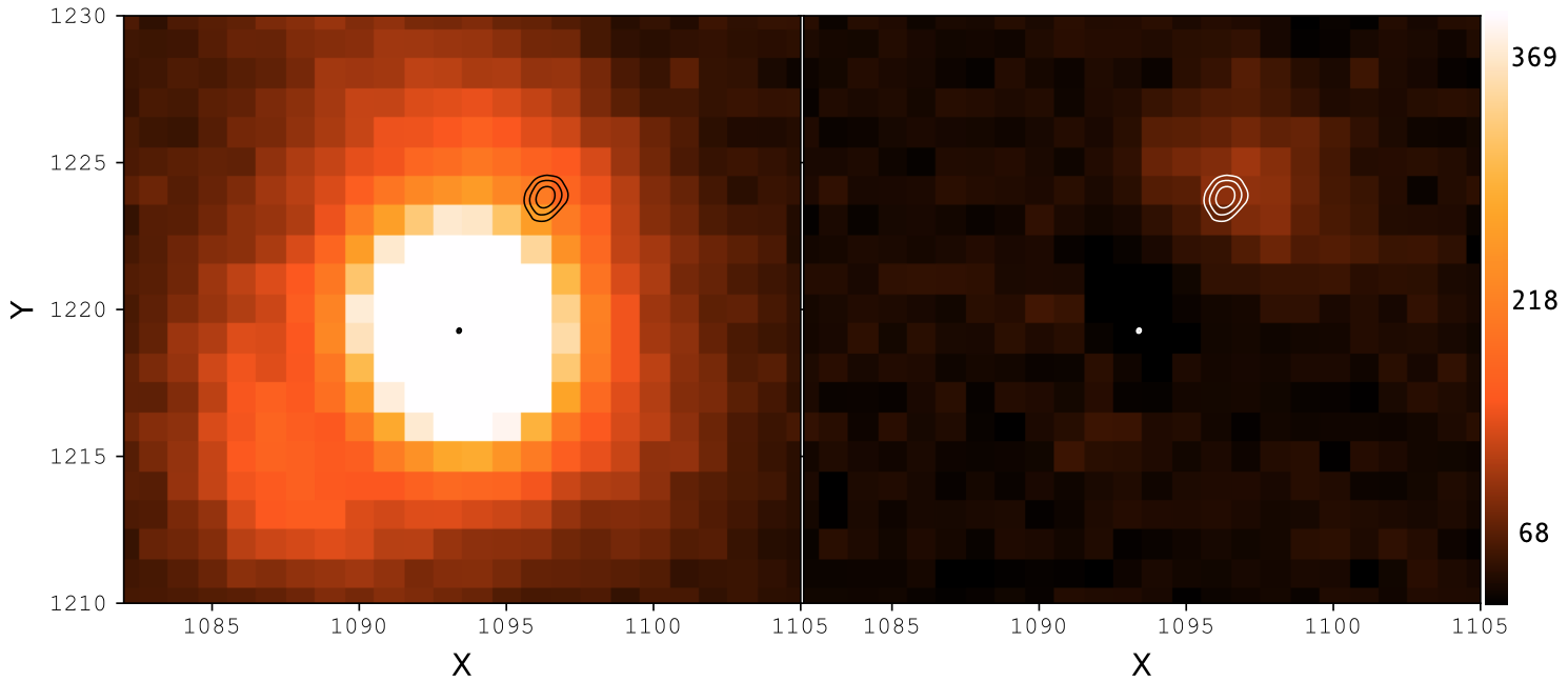
Figure 2: Best fit MCMC contours ($68.3\%$, $99.5\%$, $99.7\%$) of the lens star position and source star, with the source star being at the center of the frame. These are over-plotted on the 2020 narrow-frame Keck Osiris image (left), and the residuals of that image (right). Each frame is $\sim$ 0.2 $\times$ 0.2 arcseconds.

4 New Light Curve Model

Our detection of the exoplanet host star in the high angular resolution follow-up observations can be used to determine the masses and distance of the host star and planet only when the constraints from microlensing light curve models are also included. One common approach (Bennett et al., 2015a) is to generate a collection of model parameters that are consistent with the light curve using MCMC calculations, and then to exclude those models that are inconsistent with the high angular resolution follow-up observation results.

In cases where the modeling includes the microlensing parallax effect ($\pi_{E}$), the fraction of light curve models in the Markov Chain that are consistent with the high resolution follow-up data can be very small. This is largely because the light curve measurement of the source-lens relative proper motion constrains the direction of the $\pi_{E}$ vector to be parallel to the relative proper motion. Although $\pi_{E}$ should be present in every microlensing event observed by ground-based telescopes, it is often not included in light curve modeling analyses since it’s parameters cannot be measured very precisely. This approach can be problematic, however, because even when $\pi_{E}$ parameters cannot be measured precisely, they can still influence some of the other model parameters. Therefore, it is prudent to include $\pi_{E}$ values that are consistent with the high angular resolution follow-up data when exploring $\pi_{E}$ models. Furthermore, the event in this paper, OB161195, has a claimed $\pi_{E}$ signal from Spitzer observations, so it is helpful to compare the $\pi_{E}$ signal implied by the high angular resolution follow-up observations to the claim made based on Spitzer images.

The vast majority of models from an MCMC run (including $\pi_{E}$ models) are unlikely to be consistent with the follow-up data, which means that very long, and time consuming MCMC runs will be needed to get reasonable sampling of the light curve models consistent with the data. To address this problem, we have modified our fitting code by Bennett et al. (2010) to include the constraints from the position and brightness of the lens star identified in the Keck AO images. However, to determine the mass of the host star based on the source-lens relative proper motion (which determines $\theta_{E}$) we need to know the distance to the source star, $D_{S}$, so that the mass-distance relation, equation 3, can be used. This requires us to include $D_{S}$ as a light curve model parameter, and we use the Koshimoto et al. (2021) Galactic model to generate a prior $D_{L}$ distribution based on the $t_{E}$ measurement from a more conventional light curve model without the high angular resolution follow-up observation results. From the MCMC probability distribution we constrain the source distance, $D_{S}=8.54\pm 0.78$ kpc.

5 Planetary System Parameters

Without additional constraints (such as the lens flux from Keck) the physical parameters of a lensing system can be derived by combining two second order effects on the microlensing light curve. These are finite source effects and the microlensing parallax effect. The former provides a measurement for the source radius crossing time, $t_{*}$, which can be used to determine the angular Einstein radius, $\theta_{E}$. Therefore, a mass-distance relation can be obtained.

$$M_{L}=\frac{\theta_{E}^{2}}{\kappa\pi_{\rm rel}},\ \pi_{\rm rel}=AU\left(\frac{1}{D_{L}}-\frac{1}{D_{S}}\right),$$ (3)

where $\kappa=8.144\ \rm mas\ M_{\odot}^{-1}$. This equation has two unknowns however; lens mass and distance. If a microlensing parallax effect, $\pi_{E}$, is measured from the light curve, then an additional mass-distance relation can be obtained (Gould & Loeb, 1992), which when combined with Equation 3, yields:

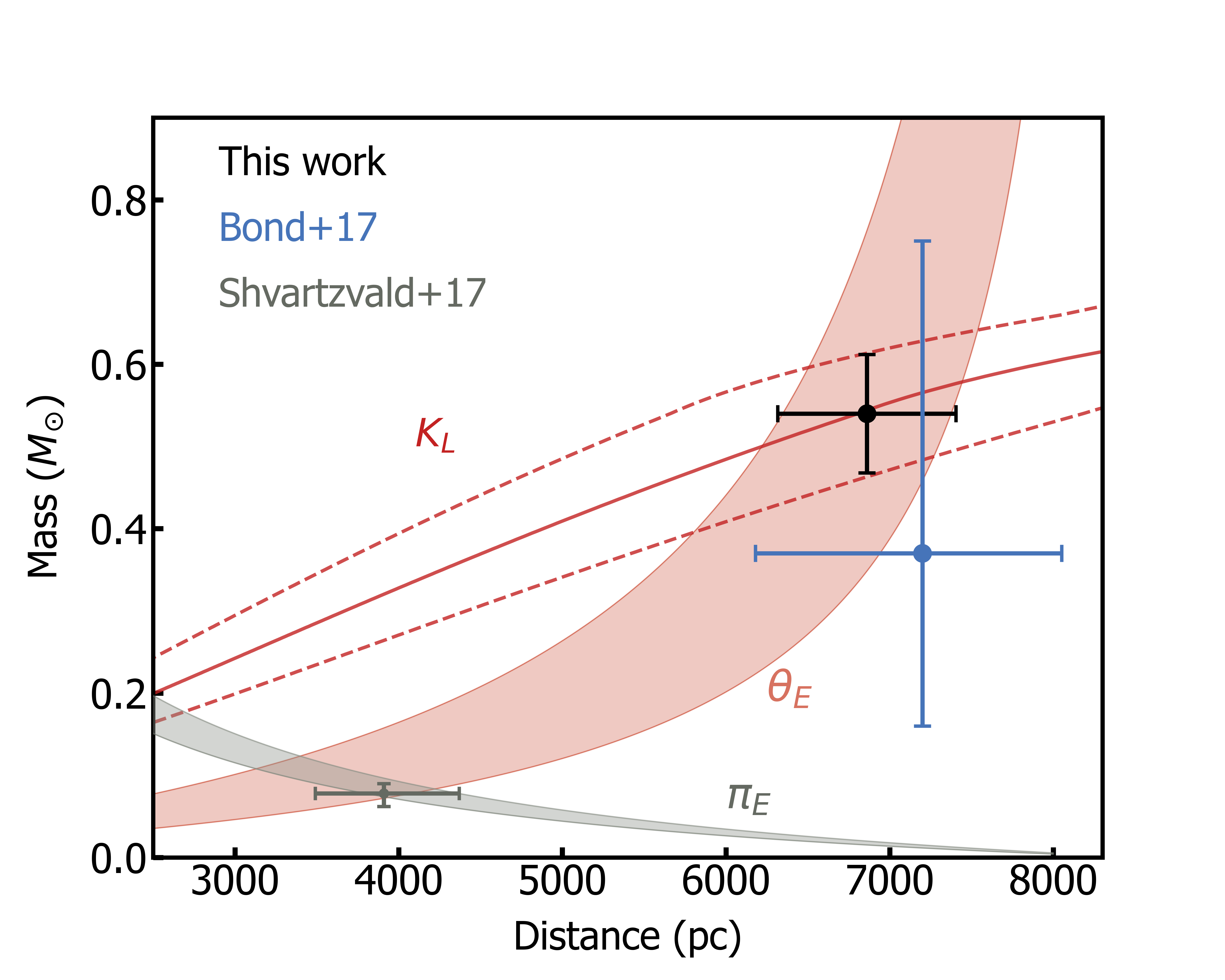
Figure 3: Mass-distance relations for OGLE-2016-BLG-1195, obtained using the Einstein ring radius ($\theta_{E}$) and the Keck K-band flux constraint ($K_{L}$). The Keck constraints are from the 2020 Osiris images. The planet-host properties are derived from the intersection of the two most reliable mass-distance relations. The host system properties estimated by B17 and S17 are shown as crosses in blue and green, respectively. The Spitzer parallax constraint obtained by S17 is shown in gray.

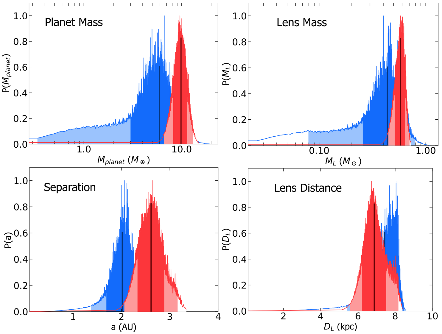
Figure 4: Bayesian posterior probability distributions for the host and planetary companion mass, their separation, and lens system distance. Using only light curve constraints are shown in blue, and with additional constraints from the follow-up Keck data in red. The center of the distributions (68.3$\%$) are shaded in dark red and blue. The remaining 95.4 $\%$ are shaded with lighter hues. The dark vertical line indicates the median of the probability distribution of each parameter.

$$M_{L}=\frac{\pi_{\rm rel}}{\kappa\pi_{E}^{2}}=\frac{\theta_{E}}{\kappa\pi_{E}}.$$ (4)

Many microlensing events do not have a measurable parallax effect though, and at best, only a projection of the parallax vector parallel to the Earth’s orbit is measured, leaving room for degeneracies. Thus, additional constraints are needed for accurate estimates of the physical parameters to be made, such as high angular resolution follow-up observations with Keck. These can be implemented from an empirical mass-luminosity relation with the measured Keck apparent magnitude. The empirical mass-luminosity relations (also used in Bennett et al. (2015b, 2016, 2018)) are from Henry & McCarthy (1993) ($M_{L}\geqslant 0.66\ M_{\odot}$), Delfosse et al. (2000) ($0.54\ M_{\odot}\geqslant M_{L}\geqslant 0.12\ M_{\odot}$) and Henry et al. (1999) ($0.10\ M_{\odot}\geqslant M_{L}\geqslant 0.07\ M_{\odot}$). The empirical mass-luminosity relation merges these three relations, smoothly interpolating between them.

In addition, since Keck can measure the source-lens proper motion, $\theta_{E}$ can be recalculated using $\theta_{E}=t_{E}\mu_{\rm rel}$. Therefore, we calculate $\theta_{E}=0.361\pm 0.015$ mas. For OB161195 we combine constraints from the empirical mass-luminosity relation and Equation 3, plotting them on a mass-distance diagram shown in Figure 3. These two relations are shown in different shades of red, with their intersection (black cross) indicating the results we find.

The final results that we use for our lens system, however, are measured by summing over the MCMC runs using a Galactic model (discussed in section 4). This model uses constraints from our $\mu_{rel}$ value (from the Keck data) and empirical mass-luminosity relations mentioned above. We run two Galactic models with different planet hosting priors (M${}^{\wedge}0$ and M${}^{\wedge}1$) and sum over the MCMC results. We compare the results of both priors, finding that the mass measurement does not vary significantly between the two. The M${}^{\wedge}0$ prior is most commonly used in Bayesian analyses of microlensing events that lack mass measurements (Bennett et al., 2014). However, more recent studies (Bennett et al. in prep, Koshimoto et al. (2021)) indicate that the probability of hosting a planet with a fixed mass ratio increases linearly with the host mass, i.e. M${}^{\wedge}1$ model. For OB161195 the final values that we use are from the M${}^{\wedge}1$ model. However, because we have a mass estimate from the Keck follow-up data, there is no significant difference between the two models.

These results are presented in Table 3 and Figure 4, where the blue histograms indicate the parameters without Keck constraints, and red histograms with Keck constraints (these are generated using the model with the M${}^{\wedge}1$ prior). Therefore, we find that the OB161195 system is a cold sub-Neptune with a mass of $M_{p}=9.91\pm 1.61\ M_{\oplus}$ orbiting a star with $M_{L}=0.57\pm 0.06\ M_{\odot}$, at a distance of $D_{L}=6.87\pm 0.65$ kpc towards the Galactic Bulge. The projected separation between planet and host is $r_{\perp}=2.62\pm 0.28$ AU, placing it beyond the snow line.

In Figure 3 we can see a graphical summary of the various conclusions for OB161195, where B17 is represented with a blue cross, S17 with gray and for this work, black. We immediately notice the drastic difference that the added parallax measurement from Spitzer has made to the physical parameters. Parallaxes are in general difficult to constrain and can result in degenerate light curves, even those obtained using Spitzer. In S17 the Spitzer light curve data have low signal-to-noise because the target is faint and covers only the trailing end. It addition, it could be affected by low level systematic errors (Koshimoto & Bennett, 2020), therefore it is necessary to investigate the Spitzer data further.

Table 3: Physical parameters from Bond et al. (2017) and Shvartzvald et al. (2017) compared to those found in this paper from the best fit MCMC values from both planet hosting priors, M${}^{\wedge}0$ and M${}^{\wedge}1$. We adopt the M${}^{\wedge}1$ values.

	M${}^{\wedge}0$	M${}^{\wedge}1$	B17	S17
$M_{L}$ ($M_{\odot}$)	0.57 $\pm$ 0.07	0.57 $\pm$ 0.06	$0.37^{+0.38}_{-0.21}$	$0.078^{+0.016}_{-0.012}$
$M_{p}$ ($M_{\oplus}$)	9.83 $\pm$ 1.62	9.91 $\pm$ 1.61	$5.10^{+5.50}_{-2.85}$	$1.43^{+0.45}_{-0.32}$
$D_{L}$ (kpc)	6.86 $\pm$ 0.65	6.87 $\pm$ 0.65	$7.20^{+0.80}_{-1.02}$	$3.19^{+0.42}_{-0.46}$
$r_{\perp}$ (AU)	2.59 $\pm$ 0.28	2.62$\pm$ 0.28	$2.01^{+0.27}_{-0.32}$	$1.16^{+0.16}_{-0.13}$

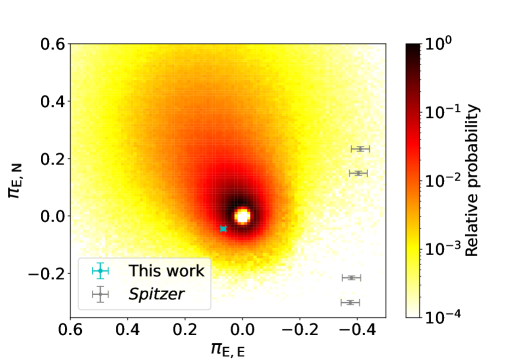
Figure 5: Two-dimensional parallax distribution for the lens in OB161195. The blue cross indicates the value obtained from this work, with constraints from Keck, and the gray crosses are the values presented in S17 using the Spitzer dataset. The color-scale shows the relative probability based on a Galactic model

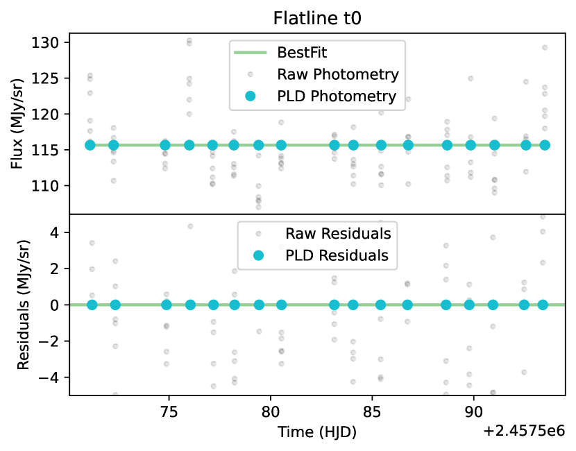
Figure 6: This is the flat line model (above panel) and residuals (below panel) from the 2019 baseline Spitzer data for OGLE-2016-BLG-1195.This model has a $\chi^{2}=120.059$.

5.1 Re-analysis of the Spitzer data

The large discrepancy between S17’s constraints on the planetary system’s physical parameters and those reported by B17 and this work, can be explained by the microlensing parallax direction presented in S17. The value they present is highly unlikely when compared to the stellar population of the Galactic disk (see Figure 5). In S17, they explain that the unlikely parallax direction (and therefore a counter-rotating lens) is a direct result of the magnification seen by Spitzer, and that high resolution imaging can resolve this issue. Using constraints from Keck the measured parallax direction would be $\pi_{E,N},\pi_{E,E}=(-0.0457\pm 0.0070),(0.0676\pm 0.0089)$. Counter-rotating low-mass stars (such as brown dwarfs) detections have been claimed before with the microlensing method (e.g. OGLE-2017-BLG-0896 Shvartzvald et al. (2019) and MOA-2015-BLG-231 Chung et al. (2019) ). Both these events however have large parallax measurements from Spitzer, which have not yet been validated with high angular resolution follow-up observations.

Therefore, we decided to re-assess the Spitzer light curve data of OB161195. Observations of this event were obtained on two occasions with Spitzer/IRAC (Fazio et al., 2004) in the 3.6 $\mu$m channel as part of the 2016 Spitzer microlensing campaign during July 12–24, 2016 at a cadence of one epoch per day. This corresponds to a total of 17 epochs with 6 dithered frames each. Additionally, 7 epochs of baseline observations of OB161195 were collected during July 12–24, 2019 at the same cadence.

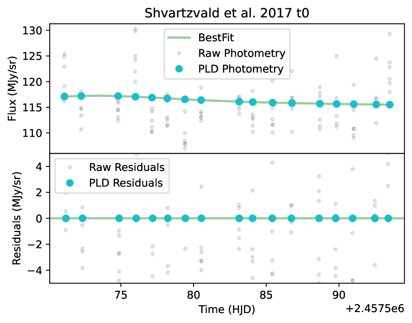
Figure 7: This is the model inferred by the Shvartzvald et al. (2017) with $t_{0}$ forced to fall in the observational gap (above panel) and the residuals (lower panel). The model has a $\chi^{2}=121.263$.

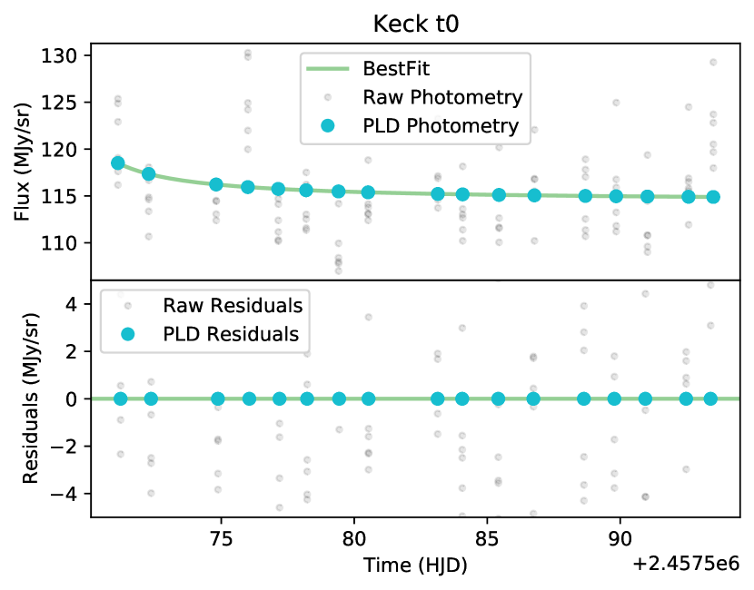
Figure 8: The predicted model from the Keck follow-up results (above panel) and residuals (lower panel). This model is the most favorable compared to the model in Figure 7 with a $\chi^{2}=102.532$.

Following Dang et al. (2020), we perform aperture photometry then model the detector systematics using Pixel Level Decorrelation (PLD), assuming a single lens and source light curve model. With such a small number of epochs, the detector systematics at each dither position are poorly sampled, so a self-calibration approach such as the PLD tends to overfit the data as suggested by the overly optimistic residuals. Consequently, the PLD analysis is inconclusive, which motivates a second look at the Spitzer frames. Nonetheless, we can compare our raw photometry with that presented in S17 which uses Calchi Novati et al. (2015)’s PSF fitting procedure.

After close inspection of our initial photometry, there is no apparent downward trend as reported by S17, which suggests that the magnification of the source is not significantly greater than the instrumental noise and the potential contamination from nearby sources. We compared the original 2016 observations with the 2019 baseline data and we note that the scatter between dithers in 2016 is systematically larger than that observed in the 2019 observations. This could be indicative that the 2016 observations either exhibit stronger instrumental systematics or that the time-variable contamination from nearby sources was more prominent. Hence, given that the source is faint and that the Spitzer magnification could be as large as the instrumental noise, if not modeled properly, we suggest that the discrepancy between the physical parameters of OB161195 inferred in this work and the results reported by S17 could be due to a poor characterization of the instrumental systematics of this particular event.

While PLD tends to overfit OB161195’s Spitzer observations, we investigate the discrepancy physical parameters inferred from S17 and our new Keck constrains by fitting 3 different light curve models to our raw photometry with a PLD correction: 1) a flat line in Figure 6, 2) a single-lens model with $t_{0}$ fixed to that reported by S17 in Figure 7, and 3) a single-lens model with $t_{0}$ fixed to that predicted from our Keck constrains 8. In this analysis, we find that the model with $t_{0}$ from S17 is disfavored, with the highest $\chi^{2}$ compared to the other models. The model that is favored when comparing $\chi^{2}$ is that from the Keck follow-up results (Figure 8), although the difference is small and not significant enough to conclude which of the two is better. Therefore, our ultimate deduction is that the Spitzer dataset is inconclusive, and the parallax yielded from such data is not a reliable avenue for a mass-measurement to be made.

6 Discussion and Conclusion

Our high angular resolution follow-up observations of the microlensing event OB161195 have allowed us to resolve the source and the lens with a separation of $\sim$ 54.5 mas. By directly measuring the lens’ K-band flux, and the amplitude and direction of the source-lens relative proper motion we have estimated the mass and distance of this planetary system. We find that OB161195 is not an ultracool dwarf orbited by an Earth-mass planet as reported by S17. Instead we find that it is a cold sub-Neptune (or super-Earth) orbiting an M-dwarf, supporting the conclusion of B17, which was reached using a Bayesian analysis with a standard Galactic model and a prior that assumes that for a mass ratio, $q$, the probability of hosting a planet is independent of the host mass. This prior assumption that is commonly used in microlensing has to be updated as described in Section 4. Their research indicates that planet detection frequency scales linearly with host mass, for a fixed mass ratio. Although the two priors differ, the final results for OB161195 (M^∧0 and M^∧1) are completely independent of the prior because we have enough measurements to constrain the masses. Cases that only have $\theta_{E}$ measurements (such as B17) are sensitive to the prior assumption.

Although OB161195 is not an ultracool dwarf as reported in Shvartzvald et al. (2017), false detections of these substellar objects could have negative implications on the understanding of their formation and evolution. Ultracool dwarfs are predicted to make up $15-30\%$ of stars in the Galaxy (Kroupa, 2001; Muzic et al., 2017), however their formation and evolution are currently only incompletely understood, since direct mass measurements are difficult to achieve for these faint objects. Techniques such as transits (e.g Carmichael et al. (2020)) and direct imaging (e.g Burgasser et al. (2006)) have had some success with ultracool dwarf binary systems, however, these methods are only sensitive to close binaries with mass ratios $q\gtrsim 0.4$. Additionally, they can only measure the total mass of the system, not the individual masses. Microlensing complements these techniques as it has the ability to detect wide-orbit binaries with low mass ratios. The individual masses can also be measured if the microlensing light curve exhibits both finite source effects and a parallax effect. With OB161195 as an example, however, parallax effects measured by Spitzer are often contaminated by systematics and/or have low signal-to-noise (Koshimoto & Bennett, 2020). Therefore, high resolution follow-up observations are the optimum solution to determine the physical properties of these low-mass ratio systems.

Parallaxes in general are not easy to measure and typically result in degenerate light curves. In the case of Spitzer parallaxes, Koshimoto & Bennett (2020) found that $>75\%$ of parallaxes obtained by the Spitzer campaign were higher than the median averages predicted by Galactic models, from a study of 50 microlens parallax measurements. They concluded that the main source of this discrepancy came from systematic errors in the Spitzer photometry. In particular Koshimoto & Bennett (2020) draw attention to this event, noting that the Spitzer light curve does not show a clear peak feature and attempts to measure a faint source star, both of which contribute to unusually high systematic errors.

A point of interest for OB161195 is its very low mass-ratio, $q=(4.25\pm 0.67)\times 10^{-5}$, because it puts it just below the estimated power law break seen in the statistical analyses of $\sim$30 microlensing planetary events by Suzuki et al. (2016, 2018). In their work they studied the measured mass ratios of events detected from 2007 to 2012 by the MOA survey, and compared them to the planet distributions from core accretion theory population synthesis models. Although the core accretion models predict planets with mass ratios $q<10^{-5}$, measurements indicate a break at $q\sim 1.7\times 10^{-4}$, indicating that we do not know the occurrence rates of planets beyond this. The precise location of the break is not well constrained, with its location more likely to be at $q=6.7^{+9.0}_{-1.8}\times 10^{-5}$. Therefore, OB161195 with $q\approx 4.25\times 10^{-5}$, is just below the mass ratio function break.

High resolution follow-up observations are crucial for accurate mass measurements of microlensing systems. In this paper we have presented the event OB161195 which had contradictory conclusions from the two detections papers, B17 and S17. Through high-resolution Keck AO data we have shown that Spitzer parallax measurements are not always a reliable mass measurement method, as they are prone to systematic errors in the photometric data when the target is faint. Low cadence observations from the space telescope can also impact the credibility of the parallax measurement. The types of planets and host stars that microlensing can detect, complement the other techniques, offering a unique window into the population and distribution of these objects in our Galaxy.

References

- Batista et al. (2014) Batista, V., Beaulieu, J.-P., Gould, A., et al. 2014, ApJ, 780
- Beaulieu (2018) Beaulieu, J.-P. 2018, Universe, 4
- Beaulieu et al. (2006) Beaulieu, J. P., Bennett, D. P., Fouqué, P., et al. 2006, Nature, 439, 437
- Beaulieu et al. (2016) Beaulieu, J. P., Bennett, D. P., Batista, V., et al. 2016, ApJ, 824, 83
- Bennett & Rhie (1996) Bennett, D. P., & Rhie, S. H. 1996, ApJ, 472, 660
- Bennett et al. (2008) Bennett, D. P., Bond, I. A., Udalski, A., et al. 2008, ApJ, 684, 663
- Bennett et al. (2010) Bennett, D. P., Rhie, S. H., Nikolaev, S., et al. 2010, ApJ, 713, 837
- Bennett et al. (2014) Bennett, D. P., Batista, V., Bond, I. A., et al. 2014, ApJ, 785, 155
- Bennett et al. (2015a) Bennett, D. P., Bhattacharya, A., Anderson, J., et al. 2015a, ApJ, 808, 169
- Bennett et al. (2015b) —. 2015b, ApJ, 808, 169
- Bennett et al. (2016) Bennett, D. P., Rhie, S. H., Udalski, A., et al. 2016, AJ, 152, 125
- Bennett et al. (2018) Bennett, D. P., Udalski, A., Bond, I. A., et al. 2018, AJ, 156, 113
- Bertin (2010) Bertin, E. 2010, SWarp: Resampling and Co-adding FITS Images Together, Astrophysics Source Code Library, ascl:1010.068
- Bertin & Arnouts (1996) Bertin, E., & Arnouts, S. 1996, A&AS, 117, 393
- Bhattacharya et al. (2018) Bhattacharya, A., Beaulieu, J. P., Bennett, D. P., et al. 2018, AJ, 156, 289
- Blackman et al. (2021) Blackman, J. W., Beaulieu, J. P., Bennett, D. P., et al. 2021, Nature, 598, 272
- Bond et al. (2001) Bond, I. A., Abe, F., Dodd, R. J., et al. 2001, MNRAS, 327, 868
- Bond et al. (2017) Bond, I. A., Bennett, D. P., Sumi, T., et al. 2017, MNRAS, 469, 2434
- Burgasser et al. (2006) Burgasser, A. J., Kirkpatrick, J. D., Cruz, K. L., et al. 2006, AJS, 166, 585
- Calchi Novati et al. (2015) Calchi Novati, S., Gould, A., Yee, J. C., et al. 2015, ApJ, 814, 92
- Carmichael et al. (2020) Carmichael, T. W., Quinn, S. N., Mustill, A. J., et al. 2020, AJ, 160, 53
- Chung et al. (2019) Chung, S.-J., Gould, A., Skowron, J., et al. 2019, ApJ, 871, 179
- Cumming et al. (2008) Cumming, A., Butler, R. P., Marcy, G. W., et al. 2008, Publications of the Astronomical Society of the Pacific, 120, 531
- Dang et al. (2020) Dang, L., Calchi Novati, S., Carey, S., & Cowan, N. B. 2020, MNRAS, 497, 5309
- Delfosse et al. (2000) Delfosse, X., Forveille, T., Ségransan, D., et al. 2000, AAP, 364, 217
- Fazio et al. (2004) Fazio, G. G., Hora, J. L., Allen, L. E., et al. 2004, ApJS, 154, 10
- Gaudi et al. (2008) Gaudi, B. S., Bennett, D. P., Udalski, A., et al. 2008, Science, 319, 927
- Gould & Loeb (1992) Gould, A., & Loeb, A. 1992, ApJ, 396, 104
- Gould et al. (2010) Gould, A., Dong, S., Gaudi, B. S., et al. 2010, ApJ, 720, 1073
- Han & Gould (1995) Han, C., & Gould, A. 1995, ApJ, 449, 521
- Henry et al. (1999) Henry, T. J., Franz, O. G., Wasserman, L. H., et al. 1999, ApJ, 512, 864
- Henry & McCarthy (1993) Henry, T. J., & McCarthy, Donald W., J. 1993, AJ, 106, 773
- Ida & Lin (2004) Ida, S., & Lin, D. N. C. 2004, ApJ, 604, 388
- Kennedy et al. (2006) Kennedy, G. M., Kenyon, S. J., & Bromley, B. C. 2006, ApJ, 650, L139
- Kim et al. (2016) Kim, S.-L., Lee, C.-U., Park, B.-G., et al. 2016, Journal of Korean Astronomical Society, 49, 37
- Koshimoto et al. (2021) Koshimoto, N., Baba, J., & Bennett, D. P. 2021, ApJ, 917, 78
- Koshimoto & Bennett (2020) Koshimoto, N., & Bennett, D. P. 2020, AJ, 160, 177
- Kroupa (2001) Kroupa, P. 2001, MNRAS, 322, 231
- Lissauer (1993) Lissauer, J. J. 1993, Annual Review of Astronomy and Astrophysics, 31, 129
- Lu et al. (2021) Lu, J. R., Gautam, A. K., Chu, D., Terry, S. K., & Do, T. 2021, Keck-DataReductionPipelines/KAI: v1.0.0 Release of KAI
- Mao & Paczynski (1991) Mao, S., & Paczynski, B. 1991, ApJ, 374, L37
- Minniti et al. (2010) Minniti, D., Lucas, P. W., Emerson, J. P., et al. 2010, New A, 15, 433
- Muzic et al. (2017) Muzic, K., Schodel, R., Scholz, A., et al. 2017, MNRAS, 471, 3699
- Quenouille (1949) Quenouille, M. H. 1949, Ann. Math. Stat., 20, 355
- Quenouille (1956) —. 1956, Biometrika, 43, 353
- Reid et al. (2002) Reid, I. N., Gizis, J. E., & Hawley, S. L. 2002, AJ, 124, 2721
- Shvartzvald et al. (2017) Shvartzvald, Y., Yee, J. C., Calchi Novati, S., et al. 2017, ApJ, 840, L3
- Shvartzvald et al. (2019) Shvartzvald, Y., Yee, J. C., Skowron, J., et al. 2019, AJ, 157, 106
- Stetson (1987) Stetson, P. B. 1987, PASP, 99, 191
- Suzuki et al. (2016) Suzuki, D., Bennett, D. P., Sumi, T., et al. 2016, ApJ, 833, 145
- Suzuki et al. (2018) Suzuki, D., Bennett, D. P., Udalski, A., et al. 2018, AJ, 155, 263
- Terry et al. (2021) Terry, S. K., Bhattacharya, A., Bennett, D. P., et al. 2021, AJ, 161, 54
- Terry et al. (2022) Terry, S. K., Bennett, D. P., Bhattacharya, A., et al. 2022, AJ, 164, 217
- Tukey (1958) Tukey, J. W. 1958, The Annals of Mathematical Statistics, 29, 581
- Udalski (2003) Udalski, A. 2003, Acta Astron., 53, 291
- Udalski et al. (1994) Udalski, A., Szymanski, M., Kaluzny, J., et al. 1994, Acta Astron., 44, 227
- Vandorou et al. (2020) Vandorou, A., Bennett, D. P., Beaulieu, J.-P., et al. 2020, AJ, 160, 121