Signaling Games with Costly Monitoring

Abstract

If in a signaling game the receiver expects to gain no information by monitoring the signal of the sender, then when a cost to monitor is implemented he will never pay that cost regardless of his off-path beliefs. This is the argument of a recent paper by T. Denti (2021). However, which pooling equilibrium does a receiver anticipate to gain no information through monitoring? This paper seeks to prove that given a sufficiently small cost to monitor any pooling equilibrium with a non-zero index will survive close to the original equilibrium.
JEL Classification: C72
Keywords: Signaling games, monitoring cost, essential equilibrium.

1 Introduction

In economic research wealth is an important variable. However, this is often not directly observable or measurable. In most sciences, these variables are replaced with a proxy, which is a variable that offers insight into this omitted variable. However, people have an incentive to misrepresent their wealth, for example, to reduce their tax burden or for prestige. How can you be sure that this signal is representative of the truth?

Signalling games are predominantly focused on how truth is preserved through a signal from an informed player to an uninformed one. Perhaps one of the most important questions derived from this is how a modification to a base signalling game changes the level of information passed on through a signal. The quantity of information that is maintained can be seen through the type of equilibrium reached.

Two types of equilibrium can occur in signaling games, pooling and separating, distinguished by the information that can be inferred from the signal. In a separating equilibrium, each of the sender’s types will choose a different message. This allows the receiver to infer the type based on the signal received and choose a best reply with complete certainty as to which type he is facing. Pooling equilibria have each type of the sender choose the same signal, making it impossible for the receiver to differentiate between the different types of the sender. Instead, the best response of the receiver will entirely rely on his belief about the distribution of the sender’s types and result in inefficient outcomes that under perfect information would never occur.

To see the importance of signaling games in game theory one has to look at its history. Non-cooperative game theory relies on the notion of complete information, that is, that there is common knowledge about the rules of the game and each player’s preferences. This severely limits the situations that the theory can be applied to and creates a large number of real-world situations that are left unexplained. However, Harsanyi (1967) showed that this theory was powerful enough to overcome these limitations, proposing a new class of games that model this incomplete information in the form of a complete information game. The Harsanyi transformation modifies the game so that one or more players can have multiple types. Each player’s type has its own unique preferences, these preferences, as well as the rules of the game, remain common knowledge. However, each player’s type is known only by the player, introducing incomplete information about the type. The simplest form of incomplete information is a signaling game, which has only one player with multiple types and, therefore, player 1’s choice of action becomes a message to help inform the other player of what type player 1 could be.

T. Denti (2021) proposes that a player’s off-path beliefs are not the sole factor in equilibrium selection, instead he suggests that if the sender anticipates an action to have zero probability of occurring then the off-path beliefs about that action can be sidestepped. This is viewed in the context of the modification of a small cost to monitor. Costly monitoring introduces the option for the receiver to either pay a price to observe the message sent by the sender or to not observe the message. This decision happens simultaneously with the sender’s selection of a message. Take a situation where the receiver expects a pooling equilibrium regardless of his decision to monitor, that is he expects to gain no information by observing the sender’s signal. Since he expects to gain no information by observing the senders signal as soon as a cost to monitor, no matter how small, is implemented the receiver will never choose to monitor the senders signal. This is not the case for every pooling equilibrium however, T. Denti (2021) does not provide a general criterion as to which pooling equilibrium will survive the introduction of monitoring costs and which will not. This paper seeks to complement T. Denti (2021) by adding further refinement as to which pooling equilibrium there will be an equilibrium sufficiently close to the original where the receiver still chooses to monitor. That is for which pooling equilibrium, equilibrium analysis would depend on off-path beliefs. This paper argues that as long as the cost-to-monitor is sufficiently small there exists a mixed equilibrium close to the original pooling equilibrium if the pooling equilibrium has a non-zero index. As the sender deviates to a separating equilibrium this creates an incentive for the receiver to monitor. This produces a mixed strategy equilibrium where the receiver monitors a proportion of the time and likewise the sender would also choose to pool some proportion of the time and separate the rest of the time. The rate at which the sender separates and the receiver chooses to not monitor increases with cost up to some threshold cost where it is no longer optimal for the receiver to monitor thus destroying the pooling equilibrium.

The contribution of this paper is to prove that all equilibria with a non-zero index will survive a sufficiently small cost to monitor and therefore through the methodology in T. Denti (2021) be selected. That is not to say that the reverse is true however as some pooling equilibrium with a zero index also have the property of being essential and therefore will survive a small cost to monitor. It does follow from the findings in this paper however that all pooling equilibria that will not be selected will have an index of zero.

1.1 Relation to the literature

T. Denti (2021) seeks to look at the role of off-path beliefs in equilibrium analysis by considering signaling games with a sufficiently small cost to monitor. The findings of this paper are that if the receiver’s off-path belief has zero probability, those beliefs can be sidestepped. When applied to signaling games, if player 2 expects a pooling equilibrium (i.e. the same message is selected regardless of player 1’s type), then player 2 will assign a probability of zero to any other message. When this game is modified by introducing costly monitoring, player 2 faces a decision to pay some cost to monitor player 1’s message. If player 2 expects a pooling equilibrium, no new information would be gained by monitoring but he would still have to pay the cost. Therefore, not monitoring will dominate monitoring. However, this is only the case for pooling equilibrium where the receiver does not believe that the sender will deviate when not monitored. The contribution of this paper is to prove that the index of pooling equilibrium is a useful tool for determining whether they survive the modification of a small cost to monitor. This paper finds that any pooling equilibrium with a non-zero index survives a sufficiently small cost to monitor with an equilibrium close to the original. The inspiration for this proof comes from an old argument in the literature about the survival of the first-mover advantage. This is primarily due to the similarity between Denti’s argument and that of Bagwell (1995).

Bagwell (1995) disputes the survival of the first-mover advantage, originally laid out by von Stackelberg (1934), when there is an error in the observation of player 1’s action. The first-mover advantage comes from players 1’s ability to commit to a strategy in a perfect information game. Player 2 will then take this action as given and pick the best response against it. Since player 2’s strategies and preferences are common knowledge, player 1 will choose to commit to the strategy where player 2’s best response maximizes her outcome, hence giving player 1 an advantage. This equilibrium will be referred to as the “Stackelberg outcome”. Importantly, this strategy is often different from the equilibrium outcome when this game is played as a simultaneous-move game. This equilibrium outcome in the simultaneous-move game is also an equilibrium of the sequential game, though not a sub-game perfect one. Bagwell disputes this notion by introducing an error in the observation of player 1’s action, that is, a small percentage of the time a signal about a different play is sent to player 2. The argument goes that player 2 will believe that any play that he sees that deviates from the “Stackelberg outcome” will be this error message and thus will continue to play his best response to the latter. This allows player 1 to then deviate to a more profitable strategy given player 2’s belief. The result of this is that the only equilibrium to survive is the equilibrium outcome of the simultaneous-move game.

The similarities between these two papers may not be immediately obvious, but if one views the Stackelberg game as containing a signal instead of complete knowledge, it becomes clearer. Both papers suggest that the response to a lack of trust in a signaling system results in that system becoming useless. For Bagwell as soon as there is some error introduced to the signal about player 1’s action, player 2 responds by not trusting any signal he gets from player 1, resulting in the equilibrium of the game reverting to that of a game without monitoring or signals. Likewise for Denti, as soon as there is a lack of faith in the signal caused by an expected pooling equilibrium, the signal is abandoned reverting to an equilibrium found in the game without monitoring or signals.

Since the cores of these papers are similar, the inspiration for this paper came from the counter arguments to Bagwell (1995). The argument against Bagwell comes primarily from two papers, van Damme and Hurkens (1994) and Güth, Kirchsteiger, and Ritzberger (1996). Van Damme and Hurkens (1994) find that Bagwell’s conclusions are reached by an over-reliance on pure strategy equilibrium. They found that instead, when the error rate is small, there is a mixed strategy equilibrium close to the original “Stackelberg outcome”. More importantly, this mixed strategy equilibrium tends towards the “Stackelberg outcome” as the error decreases. Güth, Kirchsteiger, and Ritzberger (1996) found that, although the extensive forms of the Stackelberg-game and its modification with noisy observations are not comparable, the normal forms are. The “Stackelberg outcome” was then shown to have a non-zero index. An equilibrium component with a non-zero index was then shown to always be essential, meaning that when payoffs are perturbed an equilibrium will exist close by the original component with a non-zero index. They conclude that the mixed equilibrium described by van Damme and Hurkens (1994) was instead the result of the essentiality quality of the “Stackelberg outcome” given a sufficiently small perturbation.

This paper argues that the similarity between Bagwell (1995) and T. Denti (2021) leads to a similarity in solution. By applying index theory, such as in Güth, Kirchsteiger, and Ritzberger (1996), a mixed equilibrium can be found where the choice to monitor is maintained as well as a pooling equilibrium, given a sufficiently small cost to monitor.

This paper as well as those that inspire its proof rely heavily on index theory, a mathematical topic within the study of topology. The following is a brief history of the application of index theory within game theory. For in-depth information on index theory see either McLennan (2018) or Brown (1993). Index theory was first applied to 2-player games by Shapley (1974). Later this was then generalized by Ritzberger (1994) to equilibrium components of arbitrary finite games. Gul, Pearce, and Stacchetti (1993) studied the number of regular equilibria in generic games by using index theory. Govindan and Wilson (1997, 2005) applied index theory to the study of refinement concepts. Demichelis and Germano (2000) used index theory to study the geometry of the Nash equilibrium correspondence. Demichelis and Ritzberger (2003) applied it to evolutionary game theory. Eraslan and McLennan (2013) applied it to coalitional bargaining.

This paper is split into four sections, with both sections 2 and 3 being split into two subsections. Section 2 is entitled Preliminaries and subsection 2.1 introduces all necessary notation to set up generic signaling games. Section 2.2 illustrates with an example, the beer-quiche game from Cho and Kreps (1987). Results are found in section 3.1 and in section 3.2 the methodology of the proof is applied to the beer-quiche game to once more illustrate the findings of this paper. Section 4 concludes.

2 Preliminaries

This section is broken into two parts. The first contains all relevant definitions and concepts as well as the set up for the model. The second illustrates this set up with an example.

2.1 Definitions

This paper looks at generic 2-player signaling games. The two players are referred to as player 1 or the sender and player 2 or the receiver, these terms being used interchangeably. For clarity the sender will be female (she/her) and the receiver male (he/his). A generic signaling game $G=\left(T,M,A,p,u\right)$ is specified by five objects: A finite set of types $t\in T$ assigned to player 1 by chance, a finite set of messages or signals $m\in M$ sent by player 1 conditional on her type, a finite set of actions $a\in A$ taken by player 2, a probability distribution $p:T\rightarrow\mathbb{R}_{+}$ over types (such that $\sum_{t\in T}p\left(t\right)=1$) and a payoff function $u=\left(u_{1},u_{2}\right):T\times M\times A\rightarrow\mathbb{R}^{2}$. The order of play of this game goes as follows:

1. Player 1 is assigned a type $t\in T$ according to the probability vector $p$ by chance.

2. Player 1 then observes her type and sends a message $m\in M$ to player 2 conditional on her type.

3. Player 2 observes the message, but not the type of player 1, and chooses an action $a\in A$, which ends the game.

Pure strategies for the signaling game $G$ for player 1 are $s_{1}\in S_{1}\equiv M^{T}=\left\{s:T\rightarrow M\right\}$ and for player 2 the functions $s_{2}\in S_{2}\equiv A^{M}=\left\{s:M\rightarrow A\right\}$. Mixed strategies for the signaling game $G$ are probability distributions over pure strategies. For player 1 they are denoted by:

$$\sigma_{1}\in\Delta_{1}=\left\{\sigma:M^{T}\rightarrow\mathbb{R}_{+}\left|\sum_{s\in S_{1}}\sigma\left(s\right)=1\right.\right\}$$

and for player 2 by $\sigma_{2}\in\Delta_{2}=\left\{\sigma:A^{M}\rightarrow\mathbb{R}_{+}\left|\sum_{s\in S_{2}}\sigma\left(s\right)=1\right.\right\}$. A mixed strategy profile is a pair $\sigma=\left(\sigma_{1},\sigma_{2}\right)\in\square\equiv\Delta_{1}\times\Delta_{2}$.

Any play $w$ in $G$ will be an ordered triple of type, message, and action, that is, $w=\left(t,m,a\right)\in W\equiv T\times M\times A$. An outcome for a signaling game is a probability distribution $\mu:W\rightarrow\mathbb{R}_{+}$ (such that $\sum_{\left(t,m,a\right)\in W}\mu\left(t,m,a\right)=1$) over plays that is induced by some mixed strategy profile $\sigma=\left(\sigma_{1},\sigma_{2}\right)\in\square$. The set of these outcomes will be denoted by $\Theta$.

The normal form for a signaling game $G$ is given by:

$$\Gamma=\left(S_{1}\times S_{2},u\right)$$

The definition of generic signaling games will be inspired by a result of Kreps and Wilson (1982). Their Theorem 2 states that finite generic extensive form games have only finitely many equilibrium outcomes. On the other hand, Kohlberg and Mertens (1986) showed that the set of Nash equilibria for every finite game consists of finitely many closed and connected components. It follows that in generic extensive form games, outcomes must be constant across every component of equilibrium. For, if equilibrium outcomes would vary across a component then, because the component is connected and the mapping from strategy profiles to outcomes is continuous, there would be a continuum of equilibrium outcomes. Therefore, in this paper a generic signaling game is defined as a signaling game where equilibrium outcomes are constant across every component of equilibria.

A signaling game with costly monitoring (SGCM) is a modification of the signaling game $G$: The receiver does not see the sender’s message unless he decides to pay a cost $c>0$. If he does so, he perfectly observes the sender’s message. This new game $G_{c}=\left(T,M,A,p,u,c\right)$ has an additional object $c,$ which is the decision for player 2 to pay some cost $c>0$ and monitor player 1’s action. Unlike in $G$, however, the cost to monitor ($c>0$) is subtracted from player 2’s payoffs $u_{2}$. The order of play in the SGCM is as follows:

1. Player 1 is assigned a type $t\in T$ according to the probability vector $p$ by chance.

2. Player 1 then observes her type and sends a message $m\in M$ to player 2 conditional on her type.

3. Player 2 decides simultaneously whether he would like to monitor player 1’s message for a cost $c$.

4. Player 2 then observes the message only if he has previously decided to monitor, and then chooses an action $a\in A$, ending the game. If player 2 has not monitored, he skips the observation and goes straight to picking some action.

Since the decision to monitor only affects the payoffs of player 2, player 1’s payoffs are identical in both the underlying signaling game and the SGCM. Thus player 1’s pure strategies remain the same, $S_{1}^{c}=S_{1}=M^{T}$. However, player 2’s pure strategies become the elements of $S_{2}^{c}\equiv\left\{0,1\right\}\times A^{M}\times A$. The first coordinate is the decision to monitor ($s_{21}=1$) or not ($s_{21}=0$). The second is the action conditional on the message sent by player 1. The third coordinate is the action independent of player 1’s message taken when the receiver did not monitor. Mixed strategies for the players, $\sigma_{1}\in\Delta_{1}$ and $\sigma_{2}\in\Delta_{2}^{c}=\left\{\sigma:\left\{0,1\right\}\times A^{M}\times A\rightarrow\mathbb{R}_{+}\left|\sum_{s\in S_{2}^{c}}\sigma\left(s\right)=1\right.\right\}$, and mixed strategy profiles $\sigma=\left(\sigma_{1},\sigma_{2}\right)\in\square_{c}\equiv\Delta_{1}\times\Delta_{2}^{c}$ are defined accordingly. The normal form of the SGCM $G_{c}$ is defined as:

$$\Gamma_{c}=\left(S_{1}\times S_{2}^{c},\left(u_{1},u_{2}^{c}\right)\right)$$

where $u_{2}^{c}\left(s\right)=u_{2}\left(s\right)-c\cdot s_{21}$ for all $s\in S_{1}\times S_{2}^{c}\equiv\square_{c}$.

Any play becomes a quadruple $\left(t,m,s_{21},a\right)\in W_{c}\equiv T\times M\times\left\{0,1\right\}\times A$, where $s_{21}$ is the decision to monitor given the cost. An outcome in a SGCM is a probability distribution $\mu_{c}:W_{c}\rightarrow\mathbb{R}_{+}$ (such that $\sum_{w\in W_{c}}\mu\left(w\right)=1$) that is induced by some mixed strategy profile $\sigma\in\square_{c}$. This set of outcomes will be denoted by $\Theta_{c}$. For these outcomes to project to those of the underlying signaling game the projection must integrate out the decision to monitor. Therefore, every outcome of a SGCM naturally projects to an outcome of the underlying signaling game via the function $\pi:\Theta_{c}\rightarrow\Theta$ defined by:

$$\pi\left(\mu_{c}\right)\left(t,m,a\right)=\mu_{c}\left(t,m,0,a\right)+\mu_{c}\left(t,m,1,a\right)\text{ for all }\left(t,m,a\right)\in W$$

In general, two distinct strategies of the same player are strategically equivalent if they induce the same payoffs for all players for all strategy profiles among the other players. If you reduce all strategically equivalent strategies down to a single representative for all players you create a unique purely reduced normal form. Naturally, in $G_{c}$ when player 2 chooses to not monitor he reaches an information set $h_{0}$ and chooses an action $a_{0}\in A$. Likewise the same is true when player 2 decides to monitor, he reaches an information set $h_{m}$, dependent on the message, and chooses some action $a_{m}\in A$. (Note that there are as many information sets $h_{m}$ as there are messages, but there is only one $h_{0}$). It follows that since these information sets are only reached by the decision to monitor, one information set is always unreached. This is $h_{m}$ when player 2 monitors and $h_{0}$ when he does not monitor. All strategies that differ only at the unreached information sets are strategically equivalent. All strategies that differ at $h_{0}$ when player 2 monitors are strategically equivalent, as are all strategies that differ at any $h_{m}$ when player 2 does not monitor. Collapsing strategically equivalent strategies for all players to single representatives gives the purely reduced normal form $\tilde{\Gamma}_{c}=\left(\tilde{S}_{1}\times\tilde{S}_{2}^{c},\left(u_{1},u_{2}^{c}\right)\right)$ where of course $\tilde{S}_{1}=S_{1}$. The set $\tilde{S}_{2}^{c}$ of the receiver’s pure strategies can be partitioned as follows:

$$\tilde{S}_{2}^{c} = \tilde{S}_{20}^{c}\cup\tilde{S}_{21}^{c}\text{, \ }\tilde{S}_{20}^{c}\cap\tilde{S}_{21}^{c}=\emptyset\text{,}$$

$$\tilde{S}_{20}^{c} = \left\{s_{2}\in\tilde{S}_{2}^{c}\left|s_{21}=0\right.\right\}\text{, \ }\tilde{S}_{21}^{c}=\left\{s_{2}\in\tilde{S}_{2}^{c}\left|s_{21}=1\right.\right\}$$

This partitions $\tilde{S}_{2}^{c}$ into $\tilde{S}_{20}^{c}$, the set of strategies that do not monitor and move on to $h_{0}$, and $\tilde{S}_{21}^{c}$, the set of all strategies that do monitor and thus move on to some $h_{m}$. The key observation from this is that $\tilde{S}_{21}^{c}$ is bijective to $S_{2}$, the bijection being $\left(1,\left(a_{m}\right)_{m\in M}\right)\mapsto\left(a_{m}\right)_{m\in M}$. Furthermore, each strategy in $\tilde{S}_{20}^{c}$ also correspond to strategies in $S_{2}$, those being all strategies in $S_{2}$ that act independently of the message. Those are the strategies that pick the action $a$ after every message. These strategies will give the exact same payoffs in $\tilde{S}_{20}^{c}$ as in $S_{2}$.

2.2 The Beer-Quiche Game

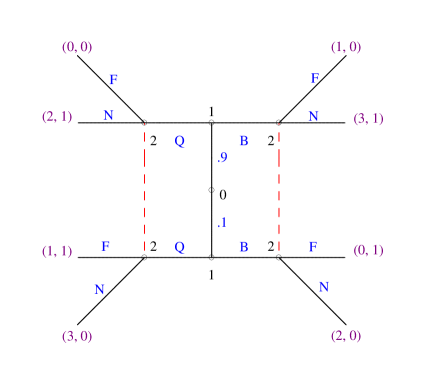
An example of a generic signaling game is the Beer-Quiche game borrowed from Cho and Kreps (1987). This game will illustrate the methodology of this paper. The Beer-Quiche game has two players, player 1 (Anne) and player 2 (Bob). Bob has the desire to duel Anne but does not know whether she is strong (S) or weak (W). He only wants to duel Anne if she is weak for he fears that otherwise he will lose. It is known by both players that Anne is the strong type 90% of the time and weak 10% of the time. Each of these types has a favorite breakfast: beer (B) for the strong type and quiche (Q) for the weak type. Bob then observes which breakfast Anne consumes and decides whether to challenge Anne to a duel (F) or not to challenge Anne to a duel (N).

	BB	BQ	QB	QQ
FF	$\begin{array}[]{cc}0.9\\ &0.1\end{array}$	$\begin{array}[]{cc}1\\ &0.1\end{array}$	$\begin{array}[]{cc}0\\ &0.1\end{array}$	$\begin{array}[]{cc}0.1\\ &0.1\end{array}$
FN	$\begin{array}[]{cc}2.9\\ &0.9\end{array}$	$\begin{array}[]{cc}2.8\\ &1\end{array}$	$\begin{array}[]{cc}0.2\\ &0\end{array}$	$\begin{array}[]{cc}0.1\\ &0.1\end{array}$
NF	$\begin{array}[]{cc}0.9\\ &0.1\end{array}$	$\begin{array}[]{cc}1.2\\ &0\end{array}$	$\begin{array}[]{cc}1.8\\ &1\end{array}$	$\begin{array}[]{cc}2.1\\ &0.9\end{array}$
NN	$\begin{array}[]{cc}2.9\\ &0.9\end{array}$	$\begin{array}[]{cc}3\\ &0.9\end{array}$	$\begin{array}[]{cc}2\\ &0.9\end{array}$	$\begin{array}[]{cc}2.1\\ &0.9\end{array}$

Table 1: Normal form of the beer-quiche game.

As in the generic signaling game previously described, the beer-quiche game is also defined by the same five objects: types, messages, actions, a probability distribution of types, and a payoff function. The sets of each of these objects are: types $T=\left\{S,W\right\}$, messages $M=\left\{B,Q\right\}$, actions $A=\left\{F,N\right\}$, and a probability distribution $p\left(S\right)=0.9$ and $p\left(W\right)=0.1$.

The order of play is as follows:

1. Anne is assigned a type, strong or weak, with the probability of “strong” being 0.9 and “weak” 0.1.

2. Anne observes her type, then chooses a breakfast, either beer or quiche.

3. Bob then observes the breakfast (message) of Anne.

4. Bob then chooses either to duel or not to duel, which ends the game.

The payoffs of this game can be seen in the extensive form shown in Figure 1, with the root being in the middle. For Anne, a payoff of 1 is granted if the favorite breakfast of her type is chosen (beer for the strong and quiche for the weak type). Anne also has a sense of self preservation, gaining a payoff of 2 for not dueling. For Bob a payoff of 1 is achieved if the weak type is dueled or the strong type is not dueled, otherwise the payoff is zero.

Figure 1: beer-quiche game in extensive form.

There are two equilibrium outcomes of this game both being pooling equilibria. The first has Anne choosing quiche (QQ) regardless of her type. Bob does not learn anything and responds by not dueling, because the probability of Anne being a strong type is high. For this equilibrium to hold, Bob must also choose to fight, when he sees Anne drink beer, with $\Pr(F\mid B)\geq 0.5$. Hence, the equilibrium component supporting the outcome $0.9\cdot\left(S,Q,N\right)+0.1\cdot\left(W,Q,N\right)$ is a 1-dimensional line segment at the boundary of the 6-dimensional strategy polyhedron. The result is an average payoff of 2.1 for Anne and 0.9 for Bob.

In the other equilibrium Anne chooses beer regardless of her type (BB). In response Bob would choose not to fight when he sees beer. Knowing that only the weak type has an incentive to deviate to quiche, he would choose to fight with probability at least one-half when he sees quiche. Hence, the equilibrium component supporting the outcome $0.9\cdot\left(S,B,N\right)+0.1\cdot\left(W,B,N\right)$ is a 1-dimensional line segment at the boundary of the 6-dimensional strategy polyhedron. The result is an average payoff of 2.9 for Anne and 0.9 for Bob. Table 1 depicts the normal form of the Beer-Quiche game, where Anne plays columns and Bob rows. (The upper left entry is Anne’s payoff and the lower right Bob’s.)

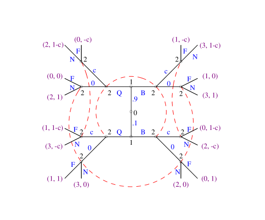
The modification of this game introduces a cost for Bob to monitor Anne’s message (breakfast). This can be imagined as any number of scenarios. For example, Anne could consumes her breakfast in private and Bob has to pay some cost $c>0$ to a private investigator to observe Anne’s breakfast. This modifies the extensive form as depicted in Figure 2. (The root is again in the middle.)

	BB	BQ	QB	QQ
CFFF	$\begin{array}[]{cc}0.9\\ &0.1-c\end{array}$	$\begin{array}[]{cc}1\\ &0.1-c\end{array}$	$\begin{array}[]{cc}0\\ &0.1-c\end{array}$	$\begin{array}[]{cc}0.1\\ &0.1-c\end{array}$
CNFF	$\begin{array}[]{cc}0.9\\ &0.1-c\end{array}$	$\begin{array}[]{cc}1\\ &0.1-c\end{array}$	$\begin{array}[]{cc}0\\ &0.1-c\end{array}$	$\begin{array}[]{cc}0.1\\ &0.1-c\end{array}$
CFFN	$\begin{array}[]{cc}2.9\\ &0.9-c\end{array}$	$\begin{array}[]{cc}2.8\\ &1-c\end{array}$	$\begin{array}[]{cc}0.2\\ &-c\end{array}$	$\begin{array}[]{cc}0.1\\ &0.1-c\end{array}$
CNFN	$\begin{array}[]{cc}2.9\\ &0.9-c\end{array}$	$\begin{array}[]{cc}1.2\\ &-c\end{array}$	$\begin{array}[]{cc}0.2\\ &-c\end{array}$	$\begin{array}[]{cc}0.1\\ &0.1-c\end{array}$
CFNN	$\begin{array}[]{cc}2.9\\ &0.9-c\end{array}$	$\begin{array}[]{cc}3\\ &0.9-c\end{array}$	$\begin{array}[]{cc}2\\ &0.9-c\end{array}$	$\begin{array}[]{cc}2.1\\ &0.9-c\end{array}$
CNNN	$\begin{array}[]{cc}2.9\\ &0.9-c\end{array}$	$\begin{array}[]{cc}3\\ &0.9-c\end{array}$	$\begin{array}[]{cc}2\\ &0.9-c\end{array}$	$\begin{array}[]{cc}2.1\\ &0.9-c\end{array}$
CFNF	$\begin{array}[]{cc}0.9\\ &0.1-c\end{array}$	$\begin{array}[]{cc}1.2\\ &-c\end{array}$	$\begin{array}[]{cc}1.8\\ &1-c\end{array}$	$\begin{array}[]{cc}2.1\\ &0.9-c\end{array}$
CNNF	$\begin{array}[]{cc}0.9\\ &0.1-c\end{array}$	$\begin{array}[]{cc}1.2\\ &-c\end{array}$	$\begin{array}[]{cc}1.8\\ &1-c\end{array}$	$\begin{array}[]{cc}2.1\\ &0.9-c\end{array}$
0FFF	$\begin{array}[]{cc}0.9\\ &0.1\end{array}$	$\begin{array}[]{cc}1\\ &0.1\end{array}$	$\begin{array}[]{cc}0\\ &0.1\end{array}$	$\begin{array}[]{cc}0.1\\ &0.1\end{array}$
0FFN	$\begin{array}[]{cc}0.9\\ &0.1\end{array}$	$\begin{array}[]{cc}1\\ &0.1\end{array}$	$\begin{array}[]{cc}0\\ &0.1\end{array}$	$\begin{array}[]{cc}0.1\\ &0.1\end{array}$
0FNF	$\begin{array}[]{cc}0.9\\ &0.1\end{array}$	$\begin{array}[]{cc}1\\ &0.1\end{array}$	$\begin{array}[]{cc}0\\ &0.1\end{array}$	$\begin{array}[]{cc}0.1\\ &0.1\end{array}$
0FNN	$\begin{array}[]{cc}0.9\\ &0.1\end{array}$	$\begin{array}[]{cc}1\\ &0.1\end{array}$	$\begin{array}[]{cc}0\\ &0.1\end{array}$	$\begin{array}[]{cc}0.1\\ &0.1\end{array}$
0NFF	$\begin{array}[]{cc}2.9\\ &0.9\end{array}$	$\begin{array}[]{cc}3\\ &0.9\end{array}$	$\begin{array}[]{cc}2\\ &0.9\end{array}$	$\begin{array}[]{cc}2.1\\ &0.9\end{array}$
0NNF	$\begin{array}[]{cc}2.9\\ &0.9\end{array}$	$\begin{array}[]{cc}3\\ &0.9\end{array}$	$\begin{array}[]{cc}2\\ &0.9\end{array}$	$\begin{array}[]{cc}2.1\\ &0.9\end{array}$
0NFN	$\begin{array}[]{cc}2.9\\ &0.9\end{array}$	$\begin{array}[]{cc}3\\ &0.9\end{array}$	$\begin{array}[]{cc}2\\ &0.9\end{array}$	$\begin{array}[]{cc}2.1\\ &0.9\end{array}$
0NNN	$\begin{array}[]{cc}2.9\\ &0.9\end{array}$	$\begin{array}[]{cc}3\\ &0.9\end{array}$	$\begin{array}[]{cc}2\\ &0.9\end{array}$	$\begin{array}[]{cc}2.1\\ &0.9\end{array}$

Table 2: Normal form for the beer quiche game with costly monitoring.

The order of play in this modified game is as follows:

1. Anne is assigned a type $t\in T=\left\{W,S\right\}$ according to the probability vector $p=\left(0.9,0.1\right)$ by chance.

2. Anne then observes her type and chooses a breakfast $m\in M=\left\{B,Q\right\}$.

3. Bob then simultaneously decides whether or not he will pay the cost $c>0$ to discover Anne’s message (breakfast).

4. Bob then observes the message only if he has previously decided to monitor; in either case he then chooses an action $a\in A$, ending the game.

This modification only alters the pure strategies of Bob, as he has the extra decision to pay the cost $c>0$ and to monitor. Anne’s pure strategies however remain unchanged. Table 2 gives the unreduced normal form of this SGCM. (Anne is the column player and Bob chooses a row, the upper left is Anne’s payoff and the lower right Bob’s.)

Figure 2: Extensive form of the Beer-Quiche game with costly monitoring.

All strategies for Bob in this normal form are functions from four information sets, $\hat{h}$, $h_{B}$, $h_{Q}$, and $h_{0}$, to choices. As there are four information sets, the values of these functions are a 4-dimentional vector, each coordinate representing a choice at one information set. Here $\hat{h}$ is the information set where Bob decides whether or not to monitor. Afterwards Bob will reach one of the remaining 3 information sets. $h_{0}$ is the information set reached when Bob does not monitor and thus does not observe a message. $h_{B}$ is the information set reached when Bob observes beer. $h_{Q}$ is the information set reached when Bob observes quiche. Each strategy can be written as a 4-dimentional vector $s_{2}\in S_{2}^{c}=\left\{0,1\right\}\times A^{\left\{B,Q\right\}}\times A$. The first coordinate is the decision to monitor $s_{21}\in\left\{0,1\right\}$ at $\hat{h}$. The second and third is the action $a\in A=\left\{F,N\right\}$ at $h_{Q}$ and $h_{B}$, respectively. The last coordinate is the action $a\in A=\left\{F,N\right\}$ at $h_{0}$.

When Bob decides not to monitor, only the information set $h_{0}$ is reached. However in Table 2 there are strategies that are differentiated by decisions at the unreached information sets $h_{B}$ and $h_{Q}$. These strategies are strategically equivalent and can be reduced as they cause the same outcome for all players, given a strategy of the opponent. The same can be said of strategies where Bob decides to monitor that differ at the unreached information set $h_{0}$. We can see, for example, that the outcomes for CFFF are identical to those for CNFF.

	BB	BQ	QB	QQ
C*FF	$\begin{array}[]{cc}0.9\\ &0.1-c\end{array}$	$\begin{array}[]{cc}1\\ &0.1-c\end{array}$	$\begin{array}[]{cc}0\\ &1-c\end{array}$	$\begin{array}[]{cc}0.1\\ &0.1-c\end{array}$
C*FN	$\begin{array}[]{cc}2.9\\ &0.9-c\end{array}$	$\begin{array}[]{cc}2.8\\ &1-c\end{array}$	$\begin{array}[]{cc}0.2\\ &-c\end{array}$	$\begin{array}[]{cc}0.1\\ &0.1-c\end{array}$
C*NF	$\begin{array}[]{cc}0.9\\ &0.1-c\end{array}$	$\begin{array}[]{cc}1.2\\ &-c\end{array}$	$\begin{array}[]{cc}1.8\\ &1-c\end{array}$	$\begin{array}[]{cc}2.1\\ &0.9-c\end{array}$
C*NN	$\begin{array}[]{cc}2.9\\ &0.9-c\end{array}$	$\begin{array}[]{cc}3\\ &0.9-c\end{array}$	$\begin{array}[]{cc}2\\ &0.9-c\end{array}$	$\begin{array}[]{cc}2.1\\ &0.9-c\end{array}$
0F**	$\begin{array}[]{cc}0.9\\ &0.1\end{array}$	$\begin{array}[]{cc}1\\ &0.1\end{array}$	$\begin{array}[]{cc}0\\ &0.1\end{array}$	$\begin{array}[]{cc}0.1\\ &0.1\end{array}$
0N**	$\begin{array}[]{cc}2.9\\ &0.9\end{array}$	$\begin{array}[]{cc}3\\ &0.9\end{array}$	$\begin{array}[]{cc}2\\ &0.9\end{array}$	$\begin{array}[]{cc}2.1\\ &0.9\end{array}$

Table 3: The reduced normal form for the beer-quiche game with costly monitoring.

This creates Table 3, the reduced normal form of the beer-quiche game with costly monitoring. In the reduced normal form all strategically equivalent strategies have been collapsed into single representatives.

Note that if we partition Bobs strategies by his decision to monitor, those strategies where he monitors are bijective to strategies in the underlying game and those strategies where Bob does not monitor are identical to strategies in the underlying game under which Bob choose the same action regardless of the breakfast he observes.

Now consider this game when the cost to monitor is zero. Strategies where Bob monitors are now identical to the underlying beer-quiche game. The pure strategies, where Bob does not monitor, are also now duplicates of the strategies where Bob chooses the same action regardless of message (breakfast) that he sees. This means that this is no longer the reduced normal form, as these strategies are strategically equivalent.

3 Equilibria

This section is broken up into two parts, the main result and an application of the result to the example.

3.1 Results

This section will prove that for every non-zero index component $C$ in a generic signaling game $G$ there exists in the modified game with costly monitoring a non-zero index component $C_{1}$ such that, so long as the monitoring cost is sufficiently small, the equilibrium outcome of the latter component will be found within a small neighborhood of the equilibrium outcome of the former.

This result is achieved by first looking at the reduced normal form of the SGCM evaluated at a cost equal to zero. This reduced normal form is also one of the possible normal forms of the underlying signaling game $G$, though with duplicate strategies. By Proposition 6.8(a) of Ritzberger (2002, p. 324) any non-zero index equilibrium component in a game with duplicate strategies will contain a component with non-zero index for the game without duplicate strategies. Therefore, a non-zero index equilibrium component of the SGCM evaluated at a cost equal to zero contains a non-zero index component of the underlying signaling game. Given that the underlying signaling game is generic, it can be deduced from Theorem 2 of Kreps and Wilson (1982) that equilibrium outcomes must be constant across every component. This implies that the equilibrium outcome of the non-zero index component in the signaling game with zero monitoring cost must project to an equilibrium outcome of the original signaling game. Given that non-zero index components are essential (Wu Wen-Tsün and Jiang Jia-He, 1962), when there is a sufficiently small monitoring cost, the projected equilibrium outcome of the signaling game with costly monitoring is close to the equilibrium outcome associated with the non-zero index components in the game without costly monitoring.

Theorem 1.

Let $G=\left(T,M,A,p,u\right)$ be a generic signaling game and $\left\{G_{c}\right\}_{c>0}$ the associated family of signaling game with costly monitoring, that is, $G_{c}=\left(T,M,A,p,u,c\right)$ with $c>0$. Then there exists an equilibrium outcome $\mu^{*}$ for $G$ such that for every $\varepsilon>0$ there is a cost $c_{\varepsilon}>0$ with the property that, whenever $0<c<c_{\varepsilon}$, there is an equilibrium outcome $\mu^{c}$ for $G_{c}$ satisfying $\left\|\pi\left(\mu^{c}\right)-\mu^{*}\right\|<\varepsilon$.

Proof.

Consider now $\tilde{\Gamma}_{0}$, that is, the reduced normal form of the SGCM but evaluated at $c=0$. This is not a reduced normal form anymore, because the strategies in $\tilde{S}_{20}^{0}$ are copies of the strategies in $\tilde{S}_{21}^{0}$ that, after observing the sender’s message, still choose the same action irrespective of the message received. Yet, $\tilde{\Gamma}_{0}$ is still a normal form game, and in fact one in which the strategies in $\tilde{S}_{21}^{0}$ are not only bijective to $S_{2}$ but also give exactly the same payoffs to both players as in $\Gamma$. That is, $\tilde{\Gamma}_{0}$ embeds $\Gamma$ and $\tilde{\Gamma}_{0}$ has the same equilibria as $\Gamma$, modulo duplicate strategies.

This implies that $\tilde{\Gamma}_{0}$ is a normal form associated with the extensive form game $G$ and with the SGCM $G_{0}$, evaluated at $c=0$. By Proposition 6.8(a) of Ritzberger (2002, p. 324) a component of equilibria with non-zero index in a game with duplicate strategies must contain a component of equilibria with non-zero index of the modified game where the duplicated strategies have been deleted. A non-zero index component $C_{0}$ in $\tilde{\Gamma}_{0}$ must therefore contain a non-zero index component $C$ of the underlying signaling game. Given that $G$ is generic, by definition equilibrium outcomes must be constant across every component. Since $\tilde{\Gamma}_{0}$ is a normal form representation of the generic extensive form game $G$, it can be concluded that all equilibrium outcomes must be constant across every equilibrium component in $\tilde{\Gamma}_{0}$. Given this, if $\mu^{*}$ is the equilibrium outcome of $C$, then the equilibrium outcome $\mu^{0}$ of $C_{0}$ must project to $\mu^{*}$, that is, $\pi\left(\mu^{0}\right)=\mu^{*}$.

By Theorem 4 of Ritzberger (1994) every component with non-zero index is essential. That is, for every $\nu>0$ there is some $\eta_{\nu}>0$ such that, so long as the perturbed game is within $\eta{}_{\nu}$ of the original, there exists an equilibrium for the perturbed game within $\nu$ from the essential component, with $\eta{}_{\nu}>0$ , $\nu>0$. Since the mapping from strategies to outcomes is continuous, for every $\epsilon>0$ there must be a $\delta{}_{\epsilon}>0$ such that strategies within $\delta_{\epsilon}$ map into outcomes within $\epsilon$. Given that an increase in cost amounts to a perturbation of payoff vectors, there exists some level of cost $c_{\epsilon}$ such that a SGCM with $0<c<c_{\epsilon}$ has a payoff vector within $\eta_{\nu}$ from $\tilde{\Gamma}_{0}$. Therefore in $\tilde{\Gamma}_{0}$, for $\epsilon>0$ choose $\delta{}_{\epsilon}>0$ such that $\left\|\sigma-\sigma^{\prime}\right\|<\delta_{\epsilon}$ implies $\left\|\mu\left(\sigma\right)-\mu\left(\sigma^{\prime}\right)\right\|<\epsilon$. Now if we take a SGCM within $\eta_{\delta_{\epsilon}}>0$ of $\tilde{\Gamma}_{0}$, then there will be an equilibrium $\sigma^{c}$ for $\tilde{\Gamma}_{c}$ such that $\min_{\sigma\in C_{0}}\left\|\sigma^{c}-\sigma\right\|<\delta_{\epsilon}$. Hence, we can deduce that since $\sigma^{c}$ is within $\delta{}_{\epsilon}$ from $C_{0}$, the equilibrium $\sigma^{c}$ must induces an outcome $\mu^{c}$ within $\epsilon$ from $\mu^{0}$. If we integrate out the decision to monitor using the projection $\pi$, it follows that $\left\|\pi\left(\mu^{c}\right)-\pi\left(\mu^{0}\right)\right\|=\left\|\pi\left(\mu^{c}\right)-\mu^{*}\right\|<\epsilon$, as desired. ∎

This result shows that the implementation of a positive cost to monitor, so long as these costs are sufficiently small, will result in an equilibrium outcome close to that of the underlying game. However, it may be possible to say more when evaluating particular classes of signaling games.

3.2 Beer-Quiche Game with Costly Monitoring

In this subsection the methodology of the proof will be applied to the Beer-Quiche example from section 2.2. The purpose is to illustrate the technique behind the result.

Recall the reduced normal form when the Beer-Quiche game with costly monitoring is evaluated at $c=0$. The strategies where Bob monitors also represent the normal form of the original game (see Table 2). The strategies where Bob does not monitor are also duplicates of strategies in the original game where Bob chooses the same action regardless of which breakfast Anne chooses.

Recall from Section 2.2 that Cho and Kreps identified two equilibrium components of the Beer-Quiche game, those being Beer Beer (BB) and Quiche Quiche (QQ). Ritzberger (1994) calculated the index for both these equilibrium components as being +1 and 0, respectively. Therefore, as the reduced normal form of the modified game at $c=0$ consists of the normal form of the underlying game with duplicate strategies, BB will also be found in the reduced normal form. This equilibrium will be the same as in the underlying game with Anne choosing Beer Beer and Bob responding by not fighting when he sees Beer and fighting 50% of the time when he sees quiche. This equilibrium will have the exact same index.

When Anne is strong, she will have an incentive to deviate to strategies that choose beer. Therefore, she chooses either BB or BQ. Given this, C*FF and C*NF are always strictly dominated by C*FN. So long as $0<c<8/10$ the strategy 0F** is strictly dominated by 0N**. Given that there is uncertainty as to the choice of the weak type to choose either beer or quiche, then C*NN is weakly dominated by C*FN. This can only be a best reply if there is certainty that Anne will only play BB. However, if this is the case for any $c>0$, both C*FN and C*NN will be strictly dominated by 0N**. Therefore, C*NN cannot be used in any equilibrium and can be discarded. In the resulting $2\times 2$ game depicted in Table 4 Bob has only the strategies C*FN and 0N**. And, if $0<c<1/10$, this $2\times 2$ game is of the Matching Pennies variety and has a unique equilibrium where both players randomize.

	$y$	$1-y$
$x$	$\begin{array}[]{cc}2.9\\ &0.9-c\end{array}$	$\begin{array}[]{cc}2.8\\ &1-c\end{array}$
$1-x$	$\begin{array}[]{cc}2.9\\ &0.9\end{array}$	$\begin{array}[]{cc}3\\ &0.9\end{array}$

Table 4: The resulting matching pennies game of the beer quiche game with costly monitoring.

At a mixed equilibrium both players must be indifferent between the pure strategies in the support. Thus, to compute the mixing probabilities, consider the indifference conditions. Those are for Anne:

$$u_{1}\left(x,1\right) =2.9\textrm{ and }u_{1}\left(x,0\right)=2.8\cdot x+3\cdot\left(1-x\right)=3-0.2\cdot x$$

$$u_{1}\left(x,1\right) =u_{1}\left(x,0\right)\Leftrightarrow x=1/2$$

Thus, to keep Anne indifferent, Bob will choose to monitor with probability of $1/2$ and fight when he sees quiche and not when he sees beer. He will also choose to not monitor and not fight with probability $1/2$. For player 2 the indifference condition is:

$$u_{2}\left(1,y\right) =0.9\cdot y+1-y-c=1-0.1\cdot y-c\textrm{ and }u_{2}\left(0,y\right)=0.9$$

$$u_{2}\left(1,y\right) =u_{2}\left(0,y\right)\Leftrightarrow y=1-10\cdot c$$

Hence, to keep Bob indifferent, Anne consumes beer irrespective of her type with probability $y=1-10\cdot c$ and chooses her preferred breakfast with probability $10\cdot c$. For this to be probabilities takes $c\leq 1/10$. As the cost $c$ goes to zero, Anne will have beer almost surely.

For a mixed strategy equilibrium to hold each player must be indifferent between each strategy. Therefore the expected payoffs of this equilibrium are identical to the BB component in the original beer-quiche game. That is an expected payoff of 2.9 for player 1 and 0.9 for player 2.

To calculate the distance between the outcomes of the original beer-quiche game and the modified game with costly monitoring one must note the probability of plays in each game. In the modified game the plays $\left(S,B,c,N\right)$ and $\left(S,B,0,N\right)$ occur with probability $0.45\cdot\left(1-10c\right)$ each. The plays $\left(W,B,c,N\right)$ and $\left(W,B,0,N\right)$ occur with probability $0.05\cdot\left(1-10c\right)$ each, the plays $\left(S,Q,c,F\right)$ and $\left(S,Q,0,N\right)$ occur with probability $4.5\cdot c$ each, and the plays $\left(W,Q,c,F\right)$ and $\left(W,Q,0,N\right)$ occur with probability $0.5\cdot c$ each. All other plays have probability zero. Integrating out the decision whether or not to monitor gives probability $0.9\cdot\left(1-10c\right)$ for the play $\left(S,B,N\right)$, probability $0.1\cdot\left(1-10c\right)$ for the play $\left(W,B,N\right)$, probabilities $4.5\cdot c$ for each of the two plays $\left(S,Q,F\right)$ and $\left(S,Q,N\right)$, and probabilities $0.5\cdot c$ for each of the two plays $\left(W,Q,F\right)$ and $\left(W,Q,N\right)$. In the original beer-quiche game the BB equilibrium induces an outcome where the play $\left(S,B,N\right)$ has probability $0.9$, the play $\left(W,B,N\right)$ has probability $0.1$, and all other plays have probability zero. Computing Euclidean distance between these two 8-dimensional vectors give $c\sqrt{123}\approx 11.1\cdot c$, which converges to zero as $c$ does.

Now take the beer-quiche game with costly monitoring when evaluated at $c>0.1$. Given that 0N** dominates 0F** and any strategy that decides to monitor is dominated by the analogous strategy that chooses not to monitor, then the pure stratergy 0N** must be an equilibrium strategy for Bob. Given this, player 1 will no longer have an incentive to pool for Bob will always choose to not monitor. This results in the separating equilibria where Anne plays beer when she is strong and quiche when she is weak, with Bob deciding not to monitor and chooses not to duel. This equilibria will have an expected payoff of 3 for Anne and 0.9 for Bob.

4 Conclusions

This paper looks at pooling equilibrium in generic signaling games when a cost to monitor is introduced. This is important because this cost to monitor represents some barrier to access information. Given that access to information in real world situations probably has some associated cost, if this destroys pooling equilibrium, it would have major consequences for the validity of pooling equilibrium in real world economic scenarios. The argument for these pooling equilibrium being destroyed are that if player 2 expects all types of player 1 to send the same message, then no information is gained by monitoring. Therefore it’s always beneficial for player 2 to not monitor no matter how small the cost is. This paper shows that in generic signaling games where a pooling equilibrium is supported in a non-zero index component, the outcome of this component survives the introduction of a sufficiently small but positive cost to monitor. Although this seems counter-intuitive, this is because all components with a non-zero index are essential. Although this paper only proves this for generic signaling games, further research may be able to prove this result for all signaling games.

References

- [1] Bagwell, K. (1995): Commitment and observability in Games, Games and Economic Behavior 8, 271-280.
- [2] Brown, R. F. (1993): "A Topological Introduction to Nonlinear Analysis", Heidelberg-New York-Dordrecht-London: Springer International.
- [3] Cho, I. K., and D. M. Kreps (1987): Signaling Games and Stable Equilibria, Quarterly Journal of Economics 102(2), 179-221.
- [4] Demichelis, S., and F. Germano (2000): On the Indices of Zeros of Vector Fields, Journal of Economic Theory 94, 192-218.
- [5] Demichelis, S., and K. Ritzberger (2003): From Evolutionary to Strategic Stability, Journal of Economic Theory 113, 51-75.
- [6] Denti, T. (2021): Costly Monitoring in Signaling Games, mimeo.
- [7] Eraslan, H., and A. McLennan (2013): Uniqueness of Stationary Equilibrium Payoffs in Coalitional Bargaining, Journal of Economic Theory 148, 2195-2222.
- [8] Govindan, S., and R. Wilson (1997): Equivalence and Invariance of the Degree and Index of Nash Equilibria, Games and Economic Behavior 21, 56-61.
- [9] Govindan, S., and R. Wilson (2005): Essential Equilibria, Proceedings of the National Academy of Sciences 102, 15706-15711.
- [10] Gul, F., D. Pearce, and E. Stacchetti (1993): A Bound on the Proportion of Pure Strategy Equilibria in Generic Games, Mathematics of Operations Research 18, 548-552.
- [11] Güth, W., G. Kirchsteiger., and K. Ritzberger (1996): Imperfectly observable commitments in n-player games, Games and Economic Behavior 23, 54-74.
- [12] Harsanyi, J. C. (1967): Games with Incomplete Information Played by "Bayesian" Players, I-III: Part I. The Basic Model, Management Science 50(12), 1804-1817.
- [13] Kohlberg, E., and J.-F. Mertens (1986): On the Strategic Stability of Equilibria, Econometrica 54(5), 1003-1037.
- [14] McLennan, A. (2018): “Advanced Fixed Point Theory for Economists,” Singapore: Springer Nature.
- [15] Kreps, D. M., and R. Wilson (1982): Sequential Equilibriuma, Econometrica 50(4), 863-894.
- [16] Ritzberger, K. (1994): The Theory of Normal Form Games from the Differentiable Viewpoint, International Journal of Game Theory 23(3), 201-236.
- [17] Ritzberger, K. (2002): “Foundations of Non-Cooperative Game Theory,” Oxford, UK: Oxford University Press.
- [18] Shapley, L. (1974): A Note on the Lemke-Howson Algorithm, Mathematical Programming Study 1, 175-189.
- [19] van Damme, E., and S. Hurkens (1994): Games with imperfectly observable commitment, Games and Economic Behavior 21, 282-308.
- [20] von Stackelberg, H. (1934): “Marktform und Gleichgewicht”, Berlin-Heidelberg: Springer Verlag.
- [21] Wu Wen-Tsün and Jiang Jia-He (1962): Essential Equilibrium Points of -Person Non-Cooperative Games, Scientia Sinica 11(10), 1307-1322.