GraphReg: Dynamical Point Cloud Registration with Geometry-aware Graph Signal Processing

Abstract

This study presents a high-accuracy, efficient, and physically induced method for 3D point cloud registration, which is the core of many important 3D vision problems. In contrast to existing physics-based methods that merely consider spatial point information and ignore surface geometry, we explore geometry aware rigid-body dynamics to regulate the particle (point) motion, which results in more precise and robust registration. Our proposed method consists of four major modules. First, we leverage the graph signal processing (GSP) framework to define a new signature, i.e.,  point response intensity for each point, by which we succeed in describing the local surface variation, resampling keypoints, and distinguishing different particles. Then, to address the shortcomings of current physics-based approaches that are sensitive to outliers, we accommodate the defined point response intensity to median absolute deviation (MAD) in robust statistics and adopt the X84 principle for adaptive outlier depression, ensuring a robust and stable registration. Subsequently, we propose a novel geometric invariant under rigid transformations to incorporate higher-order features of point clouds, which is further embedded for force modeling to guide the correspondence between pairwise scans credibly. Finally, we introduce an adaptive simulated annealing (ASA) method to search for the global optimum and substantially accelerate the registration process. We perform comprehensive experiments to evaluate the proposed method on various datasets captured from range scanners to LiDAR. Results demonstrate that our proposed method outperforms representative state-of-the-art approaches in terms of accuracy and is more suitable for registering large-scale point clouds. Furthermore, it is considerably faster and more robust than most competitors. Our implementation is publicly available at https://github.com/zikai1/GraphReg.

I Introduction

Point cloud registration is an important problem in computer vision and robotics, with many applications in various domains, such as 3D reconstruction and motion estimation, simultaneous localization and mapping (SLAM), shape recognition or retrieval, and cultural heritage. The goal is to estimate the optimal spatial transformation, including the rotation matrix $\bf{R}$ and the translation vector $\bf{t}$ (6DoF), to align two point clouds into a common coordinate system, i.e., coincide the source point cloud $\mathcal{X}$ to the target $\mathcal{Y}$ in an optimal manner (see Fig. 1 as an example).

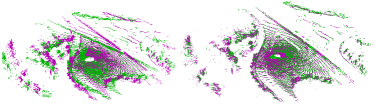
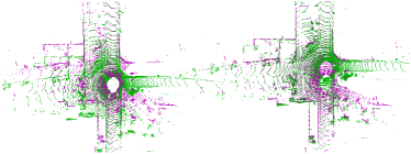
Figure 1: Registration on the large-scale KITTI LiDAR point clouds [1]. Left: Misalignment of the source (green) and the target (purple) point clouds; right: Registration by the proposed method. It achieves high-quality results with deviations less than $1^{\circ}$ ($0.1267^{\circ}$ and $0.3385^{\circ}$ of the two scenes, respectively).

The most widely used registration method, iterative closest point (ICP) [2], iteratively assumes point proximity and computes the transformation $(\mathbf{R},\mathbf{t})\in SO(3)$$\times\mathbb{R}^{3}$ by the least-squares estimator and the singular value decomposition (SVD). ICP usually performs efficiently and has high accuracy for small-scale scenarios [3]; however, it is susceptible to noise and outliers and heavily depends on the initial alignment [4]. Given its simplicity, many variants of ICP have been proposed to mitigate these problems [5]. However, a universal variant that jointly handles most registration challenges is still lacking.

Alternatively, probabilistic registration methods generalize the binary correspondence of ICP to soft assignments with probability; thus, they are more robust against outliers in principle [6, 7, 8]. The probabilistic framework commonly formulates points as the centroids of the Gaussian density functions; then, the whole point cloud is interpreted as a Gaussian mixture model (GMM). Probabilistic methods utilize kernel correlation (KC) or expectation-maximization (EM) to update the point correspondences and transformations by turns, resulting in improved robustness [9, 10]. However, these methods are typically computationally expensive and much slower than ICP-based approaches [11], especially for large-scale or high-resolution scans.

Recently, physics-based methods have shown great potential for point cloud registration [11, 3, 12], in which each point is interpreted as a particle (the terms point and particle are used synonymously), and the rigid transformation (dynamical movement) is realized through virtual forces, such as gravity or springs. These simulation methods are appealing because the force computation can be parallelized on modern GPUs, ensuring high computational efficiency. However, most of them trivially utilize the point coordinates and ignore the local surface property, such as geometry or topology, as well as the surface variation, which empirically enables high registration accuracy. In addition, they equally treat each particle and fail to handle outlier contamination, which is inevitable in practical applications. However, point clouds are typically unorganized, thus making it difficult to describe their surface properties explicitly. The present study is inspired by the impressive progress of graph signal processing (GSP) [13, 14, 15, 16], which expands classical signal processing methods to irregular graph structure [17, 18] and can effectively represent local connections among points, thus providing powerful tools for high-dimensional data analysis. In this work, we choose to leverage the GSP framework to model the surface geometry systematically and jointly consider point attributes, from which we can define useful geometric invariants, depress the outlier disturbance, boost the point-pair correspondence, and integrate them to advance the performance of dynamical point cloud registration in terms of precision, efficiency, and robustness.

Concretely, we use a Haar-like graph filter in GSP to encode the local neighbor connections of point clouds to define a new signature–point response intensity, which is closely related to the local surface geometry. We prove that the point response intensity is invariant under rigid transformations and then take it as particle mass to weigh or distinguish different particles of the many-particle system (point cloud). For efficiency, we resample points with high response intensity (keypoints) and design a novel geometric invariant based on the graph Laplacian operator from GSP [17], which is also invariant about the rotation and translation of point clouds. Critically, to make point correspondence discriminative, we combine Coulomb’s law of electrical field and the proposed geometric invariant to induce electrical forces. The registration of point clouds is then recast as solving differential equations derived from rigid-body dynamics. We also propose a novel outlier depression scheme by accommodating the point response intensity defined via GSP to robust statistics on the basis of median absolute deviation, from which most noisy outliers are successfully removed. Moreover, we introduce an adaptive simulated annealing scheme to find the global solution and considerably boost the convergence of the designed algorithm. Finally, we conduct comprehensive experiments on a wide variety of datasets to assess the performance of the proposed method with respect to precision, robustness, and efficiency. Results confirm the prominent advantages of our method over representative state-of-the-art approaches. The main contributions of this work are summarized as follows:

• We propose a novel method integrating the GSP framework with rigid-body dynamics for point cloud registration, which achieves high accuracy and efficiency.

• We use GSP to model the local surface geometry and derive new geometric invariants to estimate the correspondence confidence between point pairs with probability.

• We accommodate the proposed point response intensity to robust statistics for outlier depression, developing a highly robust and stable registration framework.

• We introduce an adaptive simulated annealing scheme to solve a globally optimal transformation, which significantly accelerates the registration process.

The rest of the paper is organized as follows: Section II reviews the point cloud registration approaches related to our study. The technical contributions of our proposed method are presented in Section III, followed by the performance evaluation on various numerical experiments in Section IV. We conclude our study, discuss the limitations, and point out possible extensions in Section V.

II Related Work

Many pioneering works have been developed for point cloud registration. We review the most relevant work in this section. Readers can refer to [19] for a comprehensive overview.

II-A ICP-based Methods

Initially, most registration methods are based on the classical ICP [2]. Over the past several decades, many variants have been proposed. For instance, to improve registration accuracy and efficiency, the original point-to-point correspondence error was replaced by other metrics such as the point-to-plane [20] distance. Zhou et al. [21] integrated color information to deduce a joint color point space, but these approaches are limited to the color property. Aiger et al. [22] extracted all coplanar 4-point congruent sets (4PCS) and aligned them between two point clouds, which is later sped up by [23] to linear time complexity using smart indexing. To circumvent the weakness of ICP that converges to the local minimum, Yang et al. [24] combined branch-and-bound (BnB) with ICP to seek the globally optimal solution exhaustively; however, the combination suffered from high complexity [25]. Another line of studies focuses on promoting robustness against noise and outliers, such as the pioneer trimmed ICP (TrICP) [26] and the use of sparsity-inducing $l_{p}~{}(p\in[0,1])$ norm [27]. Zhou et al. [28] designed a fast global registration (FGR) method with fast point feature histograms [29], and used the Geman–McClure estimator to reduce outlier influence. Recently, Yang et al. [30] combined the Truncated least-squares (TLS) Estimation And SEmidefinite Relaxation (TEASER) to register point clouds certifiably, in which outliers or spurious correspondence were restrained by TLS. Zhang et al. [31] leveraged an effective error metric Welsch’s function to achieve robust registration and proposed the fast and robust ICP (FRICP).

II-B Probabilistic Methods

Probabilistic frameworks usually use GMM to model the point cloud distribution and formulate the registration task as a density estimation problem, which can generally be categorized into KC- and EM-based methods. KC-based approaches model both point clouds. Tsin et al. [10] described both point clouds as GMMs, took KC as an affinity measure and found the transformation by minimizing Renyi’s quadratic entropy between these two distributions. Similarly, Jian et al. [6] aligned two GMMs, but the objective function was based on the $L_{2}$ distance. Instead, EM-based algorithms represent one point cloud (source) as GMM centroids and treat the other point cloud (target) as data points. Myronenko and Song [7] proposed the coherent point drift (CPD), which fitted the isotropic GMM to the target point cloud under the maximum likelihood sense, and then the correspondence and transformation were iteratively updated by EM. Horaud et al. [8] used general covariance matrices to model the Gaussian component and estimated parameters via EM-like expectation conditional maximization (ECM). As incorporate an additional uniform distribution to GMM, CPD and ECM are robust against noise and outliers. However, they require a priori setting of outlier ratio to trade off GMM and uniform distribution, which is commonly unknown in practice. In addition, probabilistic approaches are often associated with expensive computational cost, especially for large-scale point clouds.

II-C Physics-based Methods

Recently, point cloud registration analogies to physical processes are gaining much popularity. Golyanik et al. [11] took each point as a single body and moved them under a gravitational field. Similar to ICP, rotation was estimated by SVD, whereas the translation was based on the rigid-body dynamics. The method showed satisfactory results and was comparable to ICP and CPD. However, as pointed out in [12], its quadratic time complexity impeded widespread practical applications. Jauer et al. [3] designed an efficient framework based on the principle of the classical mechanics or thermodynamics and improved the registration accuracy by involving the RGB feature, although this involvement is not common for scans without color. These physics-based methods cast a new light for point cloud registration and exhibit promising results; however, most of them merely focus on spatial points, and little has been explored to integrate the more universal and effective geometric features instead of color. Moreover, they give each point, including outliers, the same weight, and the outlier-contaminated scenarios are not fully emphasized, which inevitably degrade their performance. To address these problems, in this paper, we invoke the GSP framework to capture the geometry of point clouds and develop useful geometric features to boost the accuracy, robustness, and convergence of physics-based point cloud registration.

II-D Learning-based Methods

Recent advances in deep neural networks for learning in 2D image domains have led to the development of 3D deep learning for point cloud registration. Aoki et al. [32] leveraged PointNet [33] for feature representation and adopted it into the classical image alignment algorithm, Lucas & Kanade (LK), to form a PointNetLK structure. Inspired by ICP, Wang et al. [34] designed a transformer network along with SVD for point-to-point registration. Choy et al. [35] used fully convolutional geometric features (FCGF) as keypoint descriptors, and then the pairwise correspondence between two point clouds was predicted by a 6-dimensional convolutional network, followed by the solution analogous to a weighted ICP. Deep learning-based methods embody the advantages to represent features effectively; however, at present, the main problems are from the longstanding training phase. To the best of our knowledge, the application of trained networks to multiple types of point clouds is not immediate, which is still an open challenge.

II-E GSP for Point Clouds

Signal processing on graphs generalizes the concepts and methodology from conventional signal processing theory to data indexed by the graph structure [36, 18]. GSP models each data element as a node and their relationship, such as similarity by an edge. On the basis of this construction, the concept including graph filter, spectrum ordering, and Fourier transform can be conveniently defined and applied. Benefiting from the modeling capabilities of GSP, some approaches have exploited GSP for point cloud analysis. For instance, Zhang et al. [37] conducted 3D denoising by estimating the hypergraph spectrum components and frequency coefficients of point clouds, whereas Dinesh et al. [38] designed a signal induced by a feature graph Laplacian regularizer to remove both Gaussian and Laplacian-like point cloud noise. In addition, the resampling of point clouds through the detection of high-frequency signal components has facilitated the development of point cloud storage and processing. Chen et al. [39] developed a high-pass graph filter for fast point cloud resampling, by which the visualization and shape modeling of large-scale point clouds were achieved. Deng et al. [40] went a step further and used hypergraph spectral filters to capture signal interactions of point clouds for resampling. In contrast to the above approaches, we take data points as graph nodes and particles jointly and exploit GSP for the embedding of inherent surface geometry to remove outliers and constrain the dynamical motion of particles for point cloud registration.

III Methodology

This section presents the main contributions of our study. First, GSP is customized to describe the local surface topology, followed by an effective outlier pruning method based on our proposed point response intensity. Then, graph-induced geometric invariants are used to guide the dynamical registration process. Finally, a fast global optimization scheme for maximizing energy is presented.

III-A Graph Construction

Given two point clouds with finite cardinality $\mathcal{X}=\{\bm{x}_{i}\in\mathbb{R}^{3}\}_{i=1}^{M}$ and $\mathcal{Y}=\{\bm{y}_{j}\in\mathbb{R}^{3}\}_{j=1}^{N}$, we call $\mathcal{X}$ as the source and $\mathcal{Y}$ as the target. Our purpose is to align these two point clouds into a common coordinate system. We use graph nodes to represent points and encode the local geometry of each point cloud by an adjacency matrix $\mathbf{W}\in\mathbb{R}^{M\times M}$ (take $\mathcal{X}$ as the example) with the edge weight

$$\mathbf{W}_{ij}=\left\{\begin{aligned} &e^{-\frac{\|\bm{x}_{i}-\bm{x}_{j}\|_{2}^{2}}{\sigma^{2}}},&\|\bm{x}_{i}-\bm{x}_{j}\|_{2}^{2}<\tau;\\ &0,&otherwise.\\ \end{aligned}\right.$$ (1)

Here $\|\bm{x}_{i}-\bm{x}_{j}\|_{2}$ is the Euclidean distance between $\bm{x}_{i}$ and $\bm{x}_{j}$, $\sigma$ is the variance of graph nodes, and $\tau$ is a distance threshold controlling the graph sparsity. Hereinafter, we use graphs $\mathcal{G}_{\mathcal{X}}=<\mathcal{X},\mathbf{W}_{\mathcal{X}}>$ and $\mathcal{G}_{\mathcal{Y}}=<\mathcal{Y},\mathbf{W}_{\mathcal{Y}}>$ to express point clouds and their local neighbor weights.

III-B Graph-induced Point Response Intensity

We adopt the above graph structure $\mathcal{G}_{\mathcal{X}}$, $\mathcal{G}_{\mathcal{Y}}$ and introduce graph filtering [39] to model the local surface variation of point clouds, which can be quantitatively evaluated by the following defined point response intensity $\mathcal{I}(\bm{x})$.

Specifically, let matrix $\mathbf{A}\in\mathbb{R}^{M\times M}$ be a graph-shift operator, which can be realized by the, e.g., adjacency matrix $\mathbf{W}$, transition matrix $\mathbf{D}^{-1}\mathbf{W}$, graph Laplacian matrix $\mathbf{D}-\mathbf{W}$, or other structure-related matrices, where $\mathbf{D}={\mathop{\mathrm{diag}}}(d_{1},d_{2},\cdots,d_{M})$ is the diagonal degree matrix, and $d_{i}=\sum_{\bm{x}_{j}\in\mathcal{X}}\mathbf{W}_{ij}$. Each linear and shift-invariant graph filter $h(\mathbf{A})$ is a polynomial function of $\mathbf{A}$ [17]:

$$h(\mathbf{A})=\sum_{l=0}^{L-1}h_{l}\mathbf{A}^{l}=h_{0}\mathbf{I}+h_{1}\mathbf{A}+...+h_{L-1}\mathbf{A}^{L-1},$$ (2)

where $\{h_{l}\}_{l=0}^{L-1}$ and $L$ are the coefficients and length of $h(\mathbf{A})$.

Given a general graph signal ${\color[rgb]{0,0,0}{\bm{s}(\bm{x}_{i})}}\in\mathbb{R}^{n}$ defined at the graph vertex $\bm{x}_{i}$ as an input, the graph filter $h(\mathbf{A})$ outputs another new graph signal, i.e., $h(\mathbf{A})\cdot{\color[rgb]{0,0,0}{\bm{s}(\bm{x}_{i})}}$. If $\mathbf{A}=\mathbf{D}^{-1}\mathbf{W}$, then a high-pass filter referred to as Haar-like graph filter [39] is attained $h_{Har}(\mathbf{A})=\mathbf{I}-\mathbf{A}$. Let $\mathbf{X}=[\bm{x}_{1},\bm{x}_{2},\cdots,\bm{x}_{M}]^{T}$ represent the point cloud $\mathcal{X}$, $\bm{s}(\bm{x}_{i})=\bm{x}_{i}\in\mathbb{R}^{3}$, then the new output graph signal of each ${\color[rgb]{0,0,0}{\bm{s}(\bm{x}_{i})}}$ after graph filtering is [39]

$$(h_{Har}(\mathbf{A})\cdot\mathbf{X})_{i}:=\bm{x}_{i}-\sum_{\bm{x}_{j}\in\mathcal{N}_{i}}\mathbf{A}_{ij}\bm{x}_{j},$$ (3)

where $\mathcal{N}_{i}=\{\bm{x}_{j}\in\mathcal{X}|\mathbf{W}_{ij}\neq 0\}$.

Definition 1.

The point response intensity of each point $\bm{x}_{i}$ is defined as ${\color[rgb]{0,0,0}{\mathcal{I}(\bm{x}_{i})=\|(h_{Har}(\mathbf{A})\cdot\mathbf{X})_{i}\|_{2}^{2}}}$, which reflects the local surface variation of $\bm{x}_{i}$ with respect to its neighborhoods.

Theorem 1.

The total point response intensity (local surface variation) ${\color[rgb]{0,0,0}{\mathcal{I}(\mathbf{X})={\mathop{\mathrm{diag}}}(h_{Har}(\mathbf{A})\mathbf{X}\mathbf{X}^{T}h_{Har}(\mathbf{A})^{T})\in\mathbb{R}^{M}}}$ is invariant under the rotation and translation of point clouds.

We provide all proofs in Supplemental Material.

Figure 2: Outlier depression by the proposed point response intensity $\mathcal{I}(\bm{x})$ and MAD. Left: Outlier-contaminated point clouds, where the outlier percentage of the two rows are 20% and 50%, i.e., there are separately 4,153 and 10,785+10,384=21,169 outliers in the two scenes. Right: The outlier pruning results.

III-C Outlier Depression by the Point Response Intensity

Outliers are that lie outside the overall pattern of the underlying distribution or data model [41]. To depress their adverse effect for point cloud registration, we propose to filter them out by the designed point response intensity $\mathcal{I}(\bm{x})$. The motivation is that $\mathcal{I}(\bm{x})$ can effectively describe the local surface variation, whereas outliers usually have more extreme values than correctly measured points due to their scatter properties, as illustrated in the left panel of Fig. 2. The outliers are sampled from zero mean Gaussian distribution with the standard variance determined by the size of the point cloud bounding box, with an aim to simulate the outside disturbance.

We use the X84 criterion from robust statistics [42] (pp. 64–69) to set the rejection threshold, which is based upon the median and median deviation instead of the mean and standard deviation. Benefiting from the robust location estimator median, the median absolute deviation (MAD) is defined as

$$\text{MAD}({\color[rgb]{0,0,0}{\mathcal{I}(\mathbf{X}))}}=\mathop{med}_{i=1,\cdots,M}\{|{\color[rgb]{0,0,0}{\mathcal{I}(\bm{x}_{i})}}-\mathop{med}_{j=1,\cdots,M}({\color[rgb]{0,0,0}{\mathcal{I}(\bm{x}_{j}))}}|\},$$ (4)

which is more robust than the interquartile range and typically has 50% breakdown point for the distribution scale estimation [42]. As reported in [42], the X84 criterion regulates to remove the point $\bm{x}_{i}$ with $\mathcal{I}(\bm{x}_{i})>\alpha\cdot\text{MAD}(\mathcal{I}(\mathbf{X}))$, where $\alpha=5.2$ is recommended without additional assumptions. If we assume $\mathcal{I}(\bm{x}_{i})$ satisfying Gaussian distribution, then $5.2$MAD approximately corresponds to the $3\sigma$ of Gaussian distribution, where $\sigma$ is the standard deviation [42] (p. 69). The right panel of Fig. 2 shows sample results after outlier depression. It is observed that our proposed method based on the point response intensity $\mathcal{I}(\bm{x})$ successfully removes most of the noisy outliers, hence ensuring a highly robust dynamical registration of outlier-contaminated point clouds.

III-D Graph-based Feature Description

After attaining the response intensity of each point and the elimination of outliers, we resample salient points that have high response intensity and are more discriminative of the structure feature than individual points. Using $\mathcal{I}(\bm{x})$ to resample salient points not only enables the structure similarity of two point clouds but also reduces the computational complexity, which is of practical interest. Fig. 3 presents two resampled point clouds with the model from [43].

Subsequently, we further explore the involvement of the geometric features of these high response intensity points by GSP. Suppose the graph signal ${\color[rgb]{0,0,0}{\bm{s}}}$ at $\bm{x}_{i}\in\mathcal{G}_{\mathcal{X}}$ is a vectorized normal and curvature ${\color[rgb]{0,0,0}{\bm{s}(\bm{x}_{i})}}=(n_{ix},n_{iy},n_{iz},c_{i})\in\mathbb{R}^{4}$, where $(n_{ix},n_{iy},n_{iz})$ and $c_{i}$ are the normal and curvature of $\bm{x}_{i}$, respectively. Then, the graph gradient of $\bm{s}$ at $\bm{x}_{i}$ is defined as

$$\centering\nabla_{\bm{x}_{i}}{\color[rgb]{0,0,0}{\bm{s}}}=\sum_{e_{ij}\in\mathcal{E}}\frac{\partial{{\color[rgb]{0,0,0}{\bm{s}}}}}{\partial{e_{ij}}}(\bm{x}_{i})=\sum_{\bm{x}_{j}\in\mathcal{N}_{i}}\sqrt{\mathbf{W}_{ij}}({\color[rgb]{0,0,0}{\bm{s}}}(\bm{x}_{i})-{\color[rgb]{0,0,0}{\bm{s}}}(\bm{x}_{j})),\@add@centering$$ (5)

where $\mathcal{E}$ is the set of edges connecting with $\bm{x}_{i}$. Eq. 5 reflects the variation of the local surface geometry in the neighborhood $\mathcal{N}_{i}=\{\bm{x}_{j}\in\mathcal{X}|\mathbf{W}_{ij}\neq 0\}$, inducing the graph Laplacian matrix $\mathbf{L}=\mathbf{D}-\mathbf{W}$, which is available to create another geometric invariant $\mathcal{V}_{g}(\bm{x}_{i})$.

Theorem 2.

The variation of local surface geometry $\mathcal{V}_{g}(\bm{x}_{i})$ with respect to the normals and curvatures is defined as

$$\mathcal{V}_{g}(\bm{x}_{i})=\sum_{e_{ij}\in\mathcal{E}}(\frac{\partial{{\color[rgb]{0,0,0}{\bm{s}}}}}{\partial{e_{ij}}}(\bm{x}_{i}))^{2}=\sum_{\bm{x}_{j}\in\mathcal{N}_{i}}\mathbf{W}_{ij}\|{\color[rgb]{0,0,0}{\bm{s}}}(\bm{x}_{i})-{\color[rgb]{0,0,0}{\bm{s}}}(\bm{x}_{j})\|_{2}^{2},$$ (6)

which is invariant under the rigid translation of point clouds.

(a) $M=921,753$

(b) $M/100$

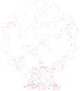
(c) $M/1000$

Figure 3: Resampling of points with high response intensity.

After graph-based resampling, we endow each point $\bm{x}_{i}$ with a response intensity $\mathcal{I}(\bm{x}_{i})$ and a geometric invariant $\mathcal{V}_{g}(\bm{x}_{i})$; both are invariant under rigid transformations. If we take $\mathcal{I}(\bm{x}_{i})$ as a lower-order statistic of the feature variation in the point level, then $\mathcal{V}_{g}(\bm{x}_{i})$ describes the higher-order variation of the local surface geometry. Fig. 4 visualizes the geometric invariant $\mathcal{V}_{g}(\bm{x})$ of two perspective point clouds via different colors, from which we observe that the similar geometry topology, such as the ear region, is with the similar $\mathcal{V}_{g}(\bm{x})$; hence, $\mathcal{V}_{g}(\bm{x})$ is an effective signature to improve the correspondence precision among pairwise points of two scans.

III-E Dynamical Registration

We use rigid-body dynamics and integrate the proposed point response intensity with geometric invariant for point cloud registration. We take points of the source $\mathcal{X}=\{\bm{x}_{i}\in\mathbb{R}^{3}\}_{i=1}^{M}$ and the target $\mathcal{Y}=\{\bm{y}_{j}\in\mathbb{R}^{3}\}_{j=1}^{N}$ as particles, and then a rotation matrix ${\bf{R}}\in SO(3)$ and a translation vector $\bf{t}\in\mathbb{R}^{3}$ exist to align these two particle systems optimally. Each particle is characterized by its mass $m_{i}$ and location $\mathbf{r}_{i}$ ($\bm{r}_{i}=\bm{x}_{i}~{}\text{or}~{}\bm{y}_{i}$). The force $\mathbf{f}_{i}$ acting on it is composed of an internal force $\bm{f}_{i}^{in}$ and an external force $\mathbf{f}_{i}^{out}$: $\bm{f}_{i}=\bm{f}_{i}^{in}+\bm{f}_{i}^{out}=\sum_{j=1}^{M}\bm{f}_{ij}^{in}+\bm{f}_{i}^{out}$, where $\bm{f}_{ij}^{in}$ is the interaction force between the $j^{th}$ and the $i^{th}$ particles in the same particle system, and $\bm{f}_{i}^{out}$ is from the outside. According to Newton’s third law [44] (or from the perspective of the law of momentum conservation), the summation of all inner forces becomes

$$\sum_{i=1}^{M}\sum_{j=1}^{M}\bm{f}_{ij}^{in}=\frac{1}{2}\sum_{i=1}^{M}\sum_{j=1}^{M}(\bm{f}_{ij}^{in}+\bm{f}_{ji}^{in})=0,$$ (7)

as $\bm{f}_{ij}^{in}=-\bm{f}_{ji}^{in}$. Therefore, the total force $\bm{f}$ exerting on the whole particle system is $\bm{f}=\sum_{i=1}^{M}\bm{f}_{i}^{out}$. In contrast to previous approaches, such as [3] that gives equal treatment of each particle and merely set their mass $m_{i}=1$, we use the point response intensity $\mathcal{I}(\bm{x})$, a natural reflection of the distribution importance, to weigh diverse particles, i.e., $m_{i}={\color[rgb]{0,0,0}{\mathcal{I}(\bm{x}_{i})}}$. Hence, the center of mass is defined as $\bm{c}=\frac{1}{G}\sum_{i=1}^{M}{\color[rgb]{0,0,0}{\mathcal{I}(\bm{x}_{i})}}\cdot\bm{r}_{i}$, where $G=\sum_{i=1}^{M}{\color[rgb]{0,0,0}{\mathcal{I}(\bm{x}_{i})}}$.

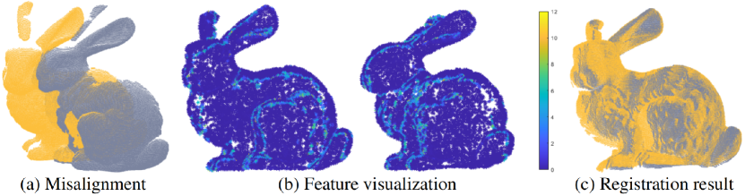
Figure 4: (a) Misalignment of two partial overlapping Bunny data [45]; (b) The geometric feature $\mathcal{V}_{g}(\bm{x})$ encoded by color is invariant under rigid transformations; (c) The registration result by the proposed method.

III-F Particle Motion

From Newton’s second law [44], the state change of the particle system, such as rotation and translation, is due to the external force $\bm{f}=\bm{a}\cdot G$, where $\bm{a}$ is the linear acceleration. In light of the kinematic equation from rigid-body dynamics, the displacement ${\color[rgb]{0,0,0}{\bm{\phi}(t)}}$ with respect to time $t$ is

$$\bm{\phi}(t)=\bm{\phi}(0)+\dot{\bm{\phi}}(0)\cdot t+\frac{1}{2}\bm{a}\cdot t^{2},$$ (8)

where $\dot{\bm{\phi}}(0)=\frac{d\bm{\phi}}{dt}|_{t=0}$ is the initial velocity. Similarly, the rotational displacement $\bm{\sigma}(t)$ is defined as

$$\bm{\sigma}(t)=\bm{\sigma}(0)+\dot{\bm{\sigma}}(0)\cdot t+\frac{1}{2}\bm{\alpha}\cdot t^{2},$$ (9)

where $\dot{\bm{\sigma}}(0)=\frac{d\bm{\sigma}}{dt}|_{t=0}$ is the initial angular velocity, and $\bm{\alpha}=\ddot{\bm{\sigma}}(0)=\frac{d^{2}\bm{\sigma}}{dt^{2}}|_{t=0}$ is the angular acceleration. Given that the source point cloud $\mathcal{X}$ is static at the beginning, we initialize $\{\bm{\phi}(0),\dot{\bm{\phi}}(0),\bm{\sigma}(0),\dot{\bm{\sigma}}(0)\}=0$. According to the theorem of angular momentum and the law of rotation [44], we have

$$\frac{d\bm{L}}{dt}=\bm{M}=J\cdot\bm{\alpha},$$ (10)

where $\bm{L}=\sum_{i=1}^{M}\tilde{\bm{x}}_{i}\times\bm{p}_{i}=\sum_{i=1}^{M}\tilde{\bm{x}}_{i}\times{\color[rgb]{0,0,0}{\mathcal{I}(\bm{x}_{i})\dot{\bm{\phi}}_{i}}}$, $\bm{M}=\sum_{i=1}^{M}\tilde{\bm{x}}_{i}\times\bm{f}_{i}^{out}$ are the summation of the angular momentum and the torque of the particle system, respectively. $\tilde{\bm{x}}_{i}=\bm{x}_{i}-\bm{c}$ is the lever from the mass center $\bm{c}$ to the point $\bm{x}_{i}$, $\bm{p}_{i}$ is the linear momentum of a particle, and $J=\sum_{i=1}^{M}{\color[rgb]{0,0,0}{\mathcal{I}}}(\bm{x}_{i})\|\tilde{\bm{x}}_{i}\|^{2}$ is the inertial moment of the system. Considering $\bm{L}=J\cdot\int\bm{\alpha}dt$, the rotational axis of the particle system is consistent with $\bm{L}$, thus we take $\frac{\bm{L}}{\|\bm{L}\|_{2}}$ as the unit rotation axis.

III-G Conversion of Vectors to Rotation Matrices

In rigid-body mechanics, the rotation of particle systems is typically represented by a vector with three parameters (Euler’s theorem [46]), i.e., a unit rotation axis $\bm{l}$ and an angle $\theta$ around it. Therefore, we utilize the Rodrigues formula [47] to convert the rotation vector to a rotation matrix for convenient representation of the point cloud registration process.

To ease the computation of the above particle motion, similar to [3], we assume stepwise motion; hence, the time interval is set as $\Delta t=1$. Therefore, Eq. 8 and 9 are simplified as $\bm{\phi}=\frac{1}{2}\bm{a},~{}\bm{\sigma}=\frac{1}{2}\bm{\alpha},~{}\text{and}~{}\bm{\alpha}=\bm{L}/J.$ For each iteration $k$, the source point cloud $\mathcal{X}$ moves toward the target $\mathcal{Y}$ under the external force induced by $\mathcal{X}$ and $\mathcal{Y}$, and the transformation is

$$\mathcal{T}_{k}=\begin{bmatrix}\bf{R}_{\theta}&\bf{t}\\ \bf{0}^{T}&1\end{bmatrix}\in SE(3),$$ (11)

where $\bf{R}_{\theta}$ is the rotation matrix with $\theta=|\bm{\sigma}|$, $\bf{t}=\bm{\phi}$ is the translation vector, and $SE(3)$ is the special Euclidean group defined as

$$SE(3)=\{\mathcal{T}=\begin{bmatrix}\bf{R}&\bf{t}\\ \bf{0}^{T}&1\end{bmatrix}\in\mathbb{R}^{4\times 4}|{\bf{R}}\in SO(3),\bf{t}\in\mathbb{R}^{3}\}.$$

III-H Geometry-aware Force Modeling

To align $\mathcal{X}$ to $\mathcal{Y}$, we adopt Coulomb’s law [48] to generate the external force acting on $\mathcal{X}$. In an electrical field, the electrostatic force $\bm{F}_{ij}$ between charged particles $Q_{i}$ and $Q_{j}$ is modeled by

$$\bm{F}_{ij}=k_{e}\frac{Q_{i}\cdot Q_{j}}{\|Q_{i}-Q_{j}\|_{2}^{2}}\cdot\frac{Q_{i}-Q_{j}}{\|Q_{i}-Q_{j}\|_{2}},$$ (12)

where the constant $k_{e}$ is the electric force constant, and $Q_{i}-Q_{j}$ is a vector pointing from $Q_{j}$ to $Q_{i}$. Analogies to Coulomb’s law, i.e., attraction between the opposite sign charges and repulsion between the same sign charges, we leverage the geometric invariant $\mathcal{V}_{g}(\bm{x})$ to guide the generation of the outer force.

Given the invariants $\mathcal{V}_{g}(\mathcal{X})=\{\mathcal{V}_{g}(\bm{x}_{1}),\cdots,\mathcal{V}_{g}(\bm{x}_{M})\}$ and $\mathcal{V}_{g}(\mathcal{Y})=\{\mathcal{V}_{g}(\bm{y}_{1}),\cdots,\mathcal{V}_{g}(\bm{y}_{N})\}$ of two 3D scans of the same object, we adopt the nearest neighbor searching (accelerated by kDtree [49]) in the feature space to generate a set of deterministic correspondences because they are invariant under rigid transformations:

$$\mathcal{C}=\{(\bm{x}_{i},\bm{y}_{j})\in\mathcal{X}\times\mathcal{Y},i\in[1,M]|\min_{j=1,\cdots,N}\|\mathcal{V}_{g}(\bm{x}_{i})-\mathcal{V}_{g}(\bm{y}_{j})\|_{2}\}.$$ (13)

Then the total outer force is defined as

$$\bm{f}=\sum_{(\bm{x}_{i},\bm{y}_{j})\in\mathcal{C}}k_{ij}\frac{\bm{y}_{j}-\bm{x}_{i}}{\|\bm{y}_{i}-\bm{x}_{i}\|_{2}^{3}}.$$ (14)

Here we use the normalized Gaussian kernel [50] $\frac{1}{\sqrt{2\pi}}exp(-\frac{\|x-y\|_{2}^{2}}{2})$ to weigh different geometric similarities, i.e., the correspondence of pairwise particles is soft with probability. To generate repulsive forces, we let

$$k_{ij}=\frac{\sqrt{2}}{\pi}exp(-\frac{\|\mathcal{V}_{g}(\bm{x}_{i})-\mathcal{V}_{g}(\bm{y}_{j})\|_{2}^{2}}{2})-1\in[-1,1].$$ (15)

Therefore, $k_{ij}$ not only encourages pairwise points with similar geometric features but also penalizes different pairs, thus enabling more valid motions of $\mathcal{X}$.

III-I Fast Transformation Solving

Given the stepwise motion, we introduce an adaptive simulated annealing (ASA) framework [51] with cool-down rate to regulate the registration process and solve for the globally optimal transformation. ASA can be considered as a variant of the gradient descent search paradigm because it incorporates uncertainties during the state transition process. In contrast to ordinary simulated annealing (SA), ASA approximates the original thermal equilibrium of SA by the D-equilibrium to accelerate the algorithm convergence, thereby considerably reducing the time consumption for point cloud registration. Moreover, ASA is almost free to tune parameters because a feedback mechanism based on the AcceptRate and LamRate is adopted to adjust the annealing temperature adaptively, rather than setting a fixed cooling schedule as implemented in SA. As in [3], we take the kinetic energy $E_{k}$ as the objective function to evaluate the registration quality of each iteration

$$E=\frac{1}{2}G\dot{\bm{x}}^{2}+\frac{1}{2}J\dot{\bm{\sigma}}^{2}.$$ (16)

The acceptance probability $P$ in ASA is defined as

$$P(\Delta E) =\frac{exp^{(-E_{k+1}/T_{k})}}{exp^{(-E_{k+1}/T_{k})}+exp^{(-E_{k}/T_{k})}}$$ (17)

$$=\frac{1}{exp(\Delta E/T_{k})+1}\approx exp(-\frac{\Delta E}{T_{k}}),$$ (18)

which essentially satisfies the Boltzmann–Gibbs distribution [3]. $T_{k}$ is the current system temperature, which is typically initialized as 1, and then updated via the composite operations with the cool down rate $c$. $\Delta E=E_{k+1}-E_{k}$ is the energy difference between consecutive states. We summarize the ASA process and our complete algorithm in Alg. 1 and Alg. 2 separately. Interested readers can refer to  [52] for further analysis of the simulated annealing framework.

Input: Current temperature $T_{k}$, $AcceptRate$, energy $E_{k}$, $E_{k-1}$, and cool-down rate $\beta\in[0.7,0.9]$.

Output: $T_{k+1}$, $AcceptRate$, $state$.

1 $state=0,\Delta E=E_{k}-E_{k-1}$.

2 if $\Delta E<0$ then

3      $AcceptRate=1/500\cdot(499\cdot AcceptRate+1)$.

4else

5       $P(\Delta E)=\min\{1,\exp^{(-\Delta E/T_{k})}\}$.

6       if $rand(0,1)<P(\Delta E)$ then

7            $AcceptRate=1/500\cdot(499\cdot AcceptRate+1)$.

8      else

9            $state=1$;

10             $AcceptRate=1/500\cdot(499\cdot AcceptRate)$.

11      

12if $k/maxNumIter<0.15$ then

13      $LamRate=0.44+0.56\cdot 560^{(-1\cdot k/(maxNumIter\cdot 0.15))}$.

14else

15       if $k/maxNumIter<0.65$ then

16            $LamRate=0.44$.

17      else

18            $LamRate=0.44\cdot 440^{-(((k/{maxNumIter})-0.65)/0.35)}$.

19      

20if $AcceptRate>LamRate$ then

21      $T_{k+1}=\beta\cdot T_{k}$.

22else

23      $T_{k+1}=T_{k}/\beta$.

Algorithm 1 Adaptive Simulated Annealing Process

Input: Two point clouds with source $\mathcal{X}$ and target $\mathcal{Y}$.

Output: Rigid transformation $\hat{\mathcal{T}}$.

1 Graph construction: $\mathcal{G}_{\mathcal{X}}$, $\mathcal{G}_{\mathcal{Y}}$, the degree matrix $\mathbf{D}$, and the adjacency matrix $\mathbf{W}$.

2 Point response intensity computation: $\mathbf{A}=\mathbf{D}^{-1}\mathbf{W}$, $h_{Har}(\mathbf{A})=\mathbf{I}-\mathbf{A}$, $\mathcal{I}(x_{i})=\|(h_{Har}(\mathbf{A})\cdot\mathbf{X})_{i}\|_{2}^{2}$.

3 Outlier removal based on the point response intensity:

4 $\text{MAD}({\color[rgb]{0,0,0}{\mathcal{I}(\mathbf{X}))}}=\mathop{med}_{i=1,\cdots,M}\{|{\color[rgb]{0,0,0}{\mathcal{I}(\bm{x}_{i})}}-\mathop{med}_{j=1,\cdots,M}({\color[rgb]{0,0,0}{\mathcal{I}(\bm{x}_{j}))}}|\}$; $\mathcal{I}(\bm{x}_{i})>\alpha\cdot\text{MAD}(\mathcal{I}(\mathbf{X}))$.

5 Resampling by $\mathcal{I}(\mathbf{X})$. Geometric invariant extraction:

6 ${\bm{s}(\bm{x}_{i})}=(n_{ix},n_{iy},n_{iz},c_{i})$;

7 $\mathcal{V}_{g}(\bm{x}_{i})=\sum_{e_{ij}\in\mathcal{E}}(\frac{\partial{{\color[rgb]{0,0,0}{\bm{s}}}}}{\partial{e_{ij}}}(\bm{x}_{i}))^{2}=\sum_{\bm{x}_{j}\in\mathcal{N}_{i}}\mathbf{W}_{ij}\|{\color[rgb]{0,0,0}{\bm{s}}}(\bm{x}_{i})-{\color[rgb]{0,0,0}{\bm{s}}}(\bm{x}_{j})\|_{2}^{2}$.

8 Geometry-aware force modeling:

9 $\mathcal{C}\!=\!\{(\bm{x}_{i},\bm{y}_{j})\in\mathcal{X}\!\times\!\mathcal{Y},i\in[1,M]|\min_{j\!=\!1,\cdots,N}\|\mathcal{V}_{g}(\bm{x}_{i})\!-\!\mathcal{V}_{g}(\bm{y}_{j})\|_{2}\}$;

10 $k_{ij}=\frac{\sqrt{2}}{\pi}exp(-\frac{\|\mathcal{V}_{g}(\bm{x}_{i})-\mathcal{V}_{g}(\bm{y}_{j})\|_{2}^{2}}{2})-1\in[-1,1]$;

11 $\bm{f}=\sum_{(\bm{x}_{i},\bm{y}_{j})\in\mathcal{C}}k_{ij}\frac{\bm{y}_{j}-\bm{x}_{i}}{\|\bm{y}_{i}-\bm{x}_{i}\|_{2}^{3}}$;

12 Initialization: $T\!=\!1$, $AcceptRate\!=\!0.5$.

13 Fast optimization, repeat until convergence:

14 Solve $\bf{t}_{k}$, $\theta_{k}$, $E_{k}$ from Eq. 8–9 and Eq. 16;

15 Update $T$, $state$, $AcceptRate$ by Algorithm 1;

16 if $state$ then

17      $\theta_{k}=\theta_{k-1}$, $\bf{t}_{k}=\bf{t}_{k-1}$, $E_{k}=E_{k-1}$;

18$\theta_{k}=\theta_{k}\cdot T$, $\bf{t}_{k}=\bf{t}_{k}\cdot T$, $\mathbf{X}=\mathcal{T}_{k}(\mathbf{X}$).

19 Transformation composite: $\hat{\mathcal{T}}=\mathcal{T}_{\texttt{maxNumIter}}\cdots\mathcal{T}_{1}$.

Algorithm 2 The Proposed GraphReg Process

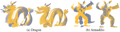
Figure 5: Misalignment of two range datasets and the registration results by the proposed method, where yellow and gray represent the target and the source point clouds, respectively.

IV Experimental Evaluations

In this section, we perform a wide variety of experiments on benchmark 3D point cloud datasets, including range scanning and LiDAR data, to show the accuracy, efficiency, and robustness of the proposed method. We compare our algorithm with seven representative methods: ICP [2] optimized in MATLAB, the modified ICP comprising point-to-point (ICP-KP) and point-to-plane (ICP-KN) metrics [53], the probabilistic registration methods including GMM [6], CPD [7], and ECM [8], and the physics-based method PIPL [3].

IV-A Implementation Details

Implementations of these compared methods are publicly available online, and their parameters are either well-tuned by ourselves or suggested by the authors. Concretely, for ICP-based methods, the KDTreeSearcher is used in MATLAB to speed up their convergence. The maximum iterations of ICP optimized in MATLAB and reimplemented by [53] are set as 200 and 50, respectively. Point normals used in point2plane minimization are found through principal component analysis (PCA) of 4-nearest-neighborhood points. The other parameters of ICP-based methods, such as params.Boundary (specifying which points are the model boundary) and params.Extrapolation (if tracing out a path in the registration state space), are set as default. For GMM [6], the following values are used:
config.motion=’rigid3d’, config.normalize=1, config.max_iter = 100, config.Lb=[-10,-10,-10,-10,-400,-400,-400], config.Ub=[10,10,10,10,400,400,400],
where normalize means transforming both point clouds to be with zero mean and unit variance before registration; Lb and Ub are the lower and upper bounds of optimization parameters. For CPD [7], its parameter settings are
opt.method=’rigid’, opt.outliers=0.5, opt.tol=1e-8, opt.normalize=1, opt.max_it=100,
here, we use the weight setting outliers=0.5 to balance the noise and outlier distribution, and the tolerance precision tol=1e-8 to determine the algorithm convergence. For ECM [8], we use maxNumIter=100. For PIPL [3], we adopt matchingMethod=’Gravitation’, $\beta\in[0.9,0.98]$, Epsilon=1e-5, temperature = 1, where $\beta$ is the cool-down rate used to regulate the system temperature, Epsilon is the lower bound of the temperature (initialized as 1) of the simulated annealing process, and the registration terminates if temperature $<$ Epsilon. In our proposed method, we use maxNumIter=100 and initialize AcceptRate = 0.5. $\tau$ in Eq. 1 is determined by the largest Euclidean distance from the 10 nearest neighbors of each point, and the variance of graph nodes $\sigma$ in $\mathbf{W}$ satisfies $\sigma^{2}=\tau^{2}/2$. We resample point clouds between the operations of outlier removal and surface normal estimation via GSP. The resampling rate is typically equal to $10\%-50\%$, with an aim to make the probabilistic approaches work within acceptable time and memory consumption. We keep the resampling rate fixed for the same point cloud.

The required surface normals and curvatures are estimated by the fast local plane fitting with 10-nearest-neighborhood points [54]. Our approach is implemented in MATLAB and all experiments are conducted on a desktop with AMD Core Ryzen 5 3600XT and 32 GB RAM.

IV-B Evaluation Measure

Following [55], we evaluate the registration quality by assessing the angular difference in degrees between two rotation matrices:

$${\mathop{\mathrm{AngErr}}}(\hat{\bf{R}},\bf{R})=\frac{180^{\circ}}{\pi}\arccos(\frac{1}{2}\{{\mathop{\mathrm{Tr}}}(\hat{\bf{R}}\bf{R}^{T})-1\}),$$ (19)

where $\hat{\bf{R}},\bf{R}\in\mathbb{R}^{3\times 3}$ are the estimated and the ground truth rotation matrices of the two point clouds, respectively; ${\mathop{\mathrm{Tr}}}(\cdot)$ is the trace operator of a matrix.

TABLE I: Average precision (degree) and runtime (second) on the Dragon and Armadillo datasets, where green and red indicate the first and the second highest accuracy, respectively.

	Dragon		Armadillo
	AngErr (∘)	Time (s)	AngErr (∘)	Time (s)
ICP [2]	0.4870	0.1921	1.8736	0.1867
ICP-KP [53]	0.6818	1.6527	1.9022	0.9715
ICP-KN [53]	0.3438	1.7171	1.6444	1.0268
GMM [6]	13.0921	34.2532	24.8091	23.2408
CPD [7]	0.6532	13.8807	0.6417	11.8751
ECM [8]	0.3438	15.6381	179.0493	10.8415
PIPL [3]	0.4412	1.1700	0.3380	1.1419
Ours	0.3323	0.3070	0.2521	0.3091

(a) Misalignment

(b) ICP (2.2052)

(c) ICP-KP (2.2052)

(d) ICP-KN (60.4347)

(e) GMM (7.8044)

(f) CPD (6.3719)

(g) ECM (2.3550)

(h) PIPL (16.6440)

(i) Ours (1.8940)

Figure 6: Registration results on the Monkey dataset [56]. Values inside the parentheses are the corresponding registration errors.

IV-C Registration on Range Datasets

IV-C1 Accuracy test

To assess the accuracy of the proposed method, we use two datasets from the Stanford 3D Scanning Repository [45], namely, Dragon and Armadillo, which are captured by a Cyberware 3030 MS laser scanner. Both datasets are scanned from two different perspectives with angle differing $24^{\circ}$ and $30^{\circ}$; therefore, they are disparate and only have partial overlappings, as illustrated in Fig. 5(a) and (b). To be statistically representative, we perform 100 registrations for each dataset.

The average accuracy and time consumption are reported in Table I. Considering that we use the proposed resampling operation to reduce the point quantity of input point clouds for all algorithms, we mainly focus on the direct registration process after the resampling step. From Table I, we conclude that the proposed method attains the highest accuracy on both datasets, and its registration speed is fast with a runtime below 1s, which is comparable to the optimized ICP in MATLAB. The baseline method PIPL attains satisfactory results but consumes more than triple time as ours. As for the probabilistic registration framework, except for CPD, GMM and ECM tend to get trapped in the local minima. In addition, probabilistic approaches suffer from long registration time, whereas ICP-based methods are more efficient. However, as angle difference increases (such as from $24^{\circ}$ to $30^{\circ}$), indicating poor initialization and low overlapping, ICP and its variants start to show more significant deviations. By contrast, the proposed method is relatively more stable. Fig. 5 exhibits the registration results of our proposed method. Further tests on Monkey dataset from EPFL Statue Model Repository [56] is presented in Fig. 6.

(a) Initialization

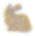
(b) PIPL (6.2240)

(c) Ours (1.4161)

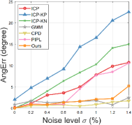
(d) AngErr

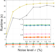
(e) Runtime

Figure 7: Comparisons of different methods with respect to the spatial noise. Top: (a) shows two noisy point clouds with zero mean and standard deviation $\sigma=0.8\%$; (b) and (c) are the alignment results by the baseline approach PIPL and the proposed method, where values inside the parenthesis are the corresponding AngErr. Bottom: Statistic results of compared methods under $\sigma\in[0\%,1.4\%]$, where our proposed method attains high precision and runs significantly fast.

Input

(a) *

ECM (0.8942)

(b) *

Input

(c) *

ECM (0.5220)

(d) *

GT

(e) *

FGR (1.3374)

(f) *

GT

(g) *

FGR (15.5914)

(h) *

TrICP (0.0115)

(i) *

TEASER++ (0.8172)

(j) *

TrICP (2.4634)

(k) *

TEASER++ (1.5666)

(l) *

GMM (21.8886)

(m) *

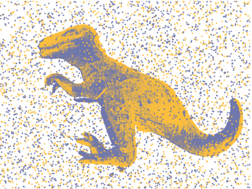
(n) FRICP (0.4695)

GMM (2.7801)

(o) *

FRICP (0.6008)

(p) *

CPD (0.2030)

(q) *

Ours (0.3540)

(r) *

CPD (0.3683)

(s) *

Ours (0.3001)

(t) *

Figure 8: Registration results of outlier-contaminated point clouds. Our method attains the highest or comparable robustness.

IV-C2 Robustness test

We contaminate the Bunny dataset from [45] with spatial noise and conduct 10 registrations to test the robustness of the proposed method. Bunny is first randomly perturbed about $30^{\circ}$ along the $X,$ $Y,$ $Z$ axes. Then, Gaussian noise with zero mean and different standard deviations $\sigma\in[0\%,1.4\%]$ relative to the three directions is added to the original 40,256 points. Fig. 7(a)-(c) show two sample point clouds with $\sigma=0.8\%$, and the corresponding registration results by PIPL and our method; our proposed algorithm shows higher robustness with lower AngErr, as indicated in the parenthesis. Fig. 7(d) and (e) summarize the registration error and running time of compared approaches (we omit ECM due to its instability and high amount of errors), in which GMM, CPD, and the proposed method attain the overall highest accuracy and outperform the others in terms of robustness. This result is attributed to the soft correspondence manner with probability. However, as observed in Fig. 7(e), GMM and CPD are much slower than our method. ICP-based methods remain efficient. However, ICP and its variants are more sensitive to noise and lead to significant errors due to the hard correspondence scheme between points.

TABLE II: Robustness test against 30% outliers on the T-rex and Parasaurolophus datasets, where the first two best results are indicated by green and red, respectively.

	T-rex		Parasaurolophus
	AngErr (∘)	Time (s)	AngErr (∘)	Time (s)
TrICP [26]	1.6420	0.9655	1.4566	1.3820
GMM [6]	10.6462	48.5120	3.0283	39.3940
CPD [7]	0.2492	41.7030	0.3905	52.4800
ECM [8]	0.4965	64.3260	0.9547	82.1900
TEASER++ [30]	0.6169	0.1362	0.7035	0.1189
FGR [28]	1.3326	0.2255	14.2750	0.1973
FRICP [31]	0.4695	1.2454	0.6008	1.2221
Ours	0.5392	0.6180	0.2455	0.5770

Subsequently, we test the robustness of the proposed method against outliers. We use TrICP [26], GMM, CPD, ECM, and three representative robust registration approaches, including FGR [28], TEASER++ [30], and FRICP [31] (all implemented in C++), for comparison, where FGR is optimized by the Open3D library [57]. We leave out PIPL due to its sensitivity to outliers. We use two partially overlapping objects from the UWA dataset [58] for assessment: T-rex and Parasaurolophus, which are acquired by a Hokuyo UTM-30LX scanning rangefinder. We randomly add 30% outliers sampled from zero mean Gaussian distribution with the standard variance relative to the bounding box size of each model, as illustrated in Fig. 8. Table II reports the average results after 10 tests, where we conclude that CPD, ECM, TEASER++, FRICP, and our method are quite robust, with deviations below $1^{\circ}$. The robustness of CPD and ECM is attributed to an additional uniform distribution except to the Gaussian mixture models, which require careful tuning of the trade-off weight. TEASER++ uses the truncated least-squares and FRICP adopts the Welsch’s function to depress spurious correspondence, thus guaranteeing high robustness. They suppress correspondence deviations during the registration process. By contrast, our method directly removes outliers according to point response intensity and the robust MAD criterion, which is free of hyperparameter tuning and can be used as preprocessing for most registration algorithms. Moreover, the proposed method with runtime below 1s is substantially faster than most competitors, especially for probabilistic-based approaches. We present several registration results in Fig. 8.

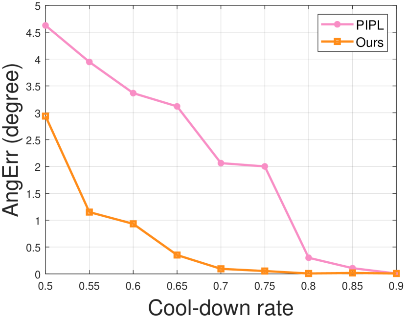
Figure 9: Left: Investigation of the cool-down rate $\beta$ for point cloud registration. Right: The misalignment point clouds and the registration result by the proposed method with $\beta=0.9$.

IV-D Effect of the Cool-down Rate

We investigate the influence of the cool-down rate $\beta$ of the (adaptive) simulated annealing for point cloud registration. We adopt the medical dataset Skeleton Hand from the Large Geometric Model Archive provided by Georgia Institute of Technology [59] for this purpose, as illustrated in the right panel of Fig. 9. The target point cloud (yellow) has 327,323 points, and the source data (gray) is attained by a random rigid transformation of the target. We vary $\beta\in[0.5,0.9]$ with $\Delta\beta=0.05$ and set the same value for PIPL and the proposed method. As observed in the left panel of Fig. 9, with $\beta$ increasing, PIPL and our method achieve higher registration accuracy. However, the proposed method outperforms PIPL by a large margin, especially under small $\beta_{s}$, due to the incorporation of local surface variation and geometric features into the force modeling. Meanwhile, our method has a broader convergence basin ($\beta\in[0.7,0.9]$) than PIPL ($\beta\in[0.85,0.9]$), suggesting a faster registration process.

IV-E Validity of the Proposed Geometric Invariant

To evaluate the validity of the proposed geometric invariant $\mathcal{V}_{g}(\bm{x})$ in our method, we utilize the Utah Teapot dataset and compare it with the baseline methods, i.e., PIPL and Super4PCS (implemented from the OpenGR C++ library [60]). As shown in Fig. 10(a), our objective is to align the pot cover (source) to the teapot (target), where the pot body is seen as outliers. Considering that the overlap ratio between the source and the target is relatively small, we make the overlap setting $O$ (a hyperparameter) of Super4PCS belong to $\{0.20,0.50\}$. $O=0.20$ represents a relatively conservative overlap rate, whereas $O=0.50$ gives a more confident estimation. To be statistically representative, we vary $\beta\in\{0.9,0.95\}$, perform 100 trials and measure the average deviation and runtime, as reported in Table III. Super4PCS and PIPL show significant errors as the ambiguous outliers disturb their correspondence between point pairs. By contrast, our method attains substantially accurate registration because the geometric invariant $\mathcal{V}_{g}(\bm{x})$ provides more insights into the point clouds’ feature distribution than the single point location, hence enabling more correct correspondence. In addition, with the priori overlap threshold $O$ increasing, Super4PCS consumes more time but without accuracy enhancement, whereas our method outperforms Super4PCS and PIPL in terms of speed. We present a test sample in Fig. 10(c) and provide a demo in Supplemental Material to exhibit this dynamical registration process.

(a) Initialization

(b) Super4PCS

(c) PIPL

(d) Ours

Figure 10: Verification of the proposed geometric invariant $\mathcal{V}_{g}(\bm{x})$. Our proposed method attains higher registration accuracy and speed than Super4PCS and PIPL.

	$\beta=0.90$ $(O=0.20)$		$\beta=0.95$ $(O=0.50)$
	AngErr (∘)	Time (s)	AngErr (∘)	Time (s)
Super4PCS [23]	40.4707	0.6690	40.4646	1.3258
PIPL [3]	50.8282	0.4460	49.9012	0.6085
Ours	0.0004	0.3210	0.0003	0.2960

TABLE III: Statistic of the average angle error and runtime on the Utah TeaPot dataset.

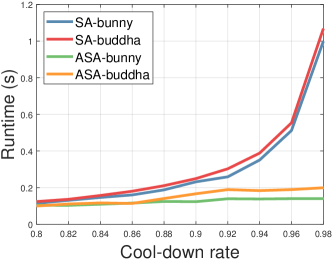
Figure 11: Runtime comparison of the simulated annealing (SA) and the adaptive simulated annealing (ASA) algorithms for point cloud registration. ASA is much faster and more stable than SA, especially under large cool-down rates.

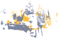
Figure 12: Examples of the large-scale terrestrial laser scanning point clouds captured from different perspectives.

IV-F Comparison of SA & ASA

To test the acceleration effect of the introduced adaptive simulated annealing (ASA) method for point cloud registration, we further compare it with the simulated annealing (SA) algorithm. For this purpose, we replace the global optimization part with SA and keep the others fixed in our method. SA requires a low or cooling temperature Epsilon to judge the convergence and stop the algorithm iteration. We adopt the typical default setting Epsilon=1e-5 for the test. By contrast, ASA uses the maxNumIter as the termination condition, where we set maxNumIter=100.

TABLE IV: Quantitative results on the ETH Facade dataset. Green and red fonts indicate the first two best accuracy.

	Metric	ICP[2]	ICP-KP[53]	ICP-KN[53]	GMM[6]	CPD[7]	ECM[8]	TEASER++[30]	FGR[28]	FRICP[31]	PIPL[3]	Ours
Pair 1	AngErr	11.6826	12.7025	9.1673	20.1567	2.6700	5.9759	1.8652	4.2284	2.4306	4.1883	1.6100
	Time	0.3285	3.8016	3.9138	38.4033	47.0350	39.6100	1.193	0.5711	0.8287	0.4504	0.3584
Pair 2	AngErr	2.8705	2.9106	4.0623	4.7727	2.5726	0.3724	0.8146	1.6893	2.8869	0.1031	0.0839
	Time	0.2226	2.8928	2.9664	42.4362	26.9683	30.8803	0.7606	0.3654	0.7960	0.5380	0.3357
Pair 3	AngErr	5.4316	5.4488	9.4825	6.9385	13.4760	11.9003	2.3320	1.6398	0.4207	3.9591	1.9209
	Time	0.2301	2.9445	3.0095	68.5586	24.2632	31.8921	0.9601	0.4571	0.7540	0.5303	0.3415
Pair 4	AngErr	2.0054	2.0283	3.3633	5.9180	9.9122	12.2728	5.3606	0.8089	2.7742	10.1872	1.6625
	Time	0.2156	2.3750	2.4604	38.6081	37.4666	26.2225	0.7401	0.3609	0.5212	0.4461	0.3419
Pair 5	AngErr	6.0332	6.0734	7.2193	20.9932	8.1589	7.3281	4.2966	2.1304	1.8182	5.9874	1.3293
	Time	0.2349	2.2919	2.3802	23.7734	18.4693	25.5012	0.8913	0.4588	0.7080	0.4495	0.3412

(a) ICP (10.2077)

(b) ICP-KP (5.7161)

(c) ICP-KN (26.4846)

(d) GMM (15.3665)

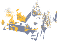
(e) CPD (2.5504)

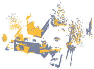
(f) ECM (2.9128)

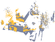
(g) TEASER++ (3.0316)

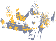
(h) FGR (3.1425)

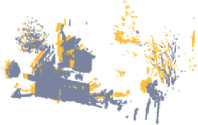
(i) FRICP (2.4328)

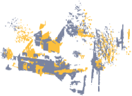
(j) PIPL (5.8498)

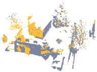
(k) Ours (2.3639)

Figure 13: Qualitative results on the TLS Facade dataset. The proposed method attains the highest precision than competitors.

We use the Bunny and the Buddha datasets from [45] for comparison, where the point number of the source and target point clouds of Buddha is 78,056 and 75,582, respectively. To be fair, we vary the cool-down rate $\beta\in[0.8,0.98]$ with interval $\Delta\beta=0.02$ and report the average results of 10 trials. The average runtime is reported in Fig. 11. As shown in the figure, SA consumes more time than ASA for both datasets, and with $\beta$ increasing, its runtime grows significantly. However, ASA remains relatively stable due to the adaptive tuning scheme of the temperature, and its time consumption remains below $0.2s$ even at large $\beta$. We present the Buddha registration results after algorithm convergence in Fig. 14.

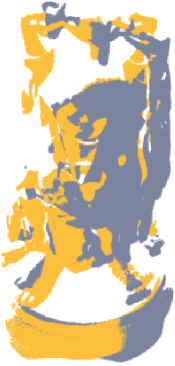
(a)

(b)

(c)

(d)

Figure 14: (a) The input two misalignment point clouds. (b)–(c) Registration results of SA and ASA with AngErr=5.2386 and AngErr=0.4301, separately. (d) The ground truth alignment.

TABLE V: Statistic of the registration results on KITTI odemetry datasets, where the average deviations of the relative rotation (Rel. Rot.), relative translation (Rel. Tran.), absolute rotation (Abs. Rot.), absolute translation (Abs. Tran.), last frame rotation (Last Rot.), and last frame translation (Last Tran.) are reported. Values inside the parenthesis indicate the maximum. Blue and orange fonts indicate the first two highest accuracy.

	Rel. Rot. (∘)	Rel. Tran. (m)	Abs. Rot. (∘)	Abs. Tran. (m)	Last Rot. (∘)	Last Tran. (m)
ICP[2]	0.2850 (2.6499)	0.2978 (5.4468)	21.9215 (39.8268)	79.6718 (213.1728)	39.8268	213.1728
ICP-KP [53]	0.2830 (2.5197)	0.2930 (3.6881)	21.9874 (38.9154)	79.7293 (212.3571)	38.7033	212.3571
ICP-KN [53]	1.4763 (9.3142)	0.3019 (5.0016)	139.0011 (179.7096)	190.6753 (496.8816)	126.6452	496.8816
GMM [6]	0.3326 (1.0954)	2.9138 (4.7576)	25.8011 (40.7604)	227.1595 (497.6106)	40.093	497.6106
CPD [7]	0.2092 (1.0069)	0.2161 (1.0037)	13.7057 (24.7993)	35.6197 (95.2179)	24.4202	94.8900
ECM [2]	0.1264 (2.5036)	0.1912 (3.6157)	5.3706 (12.2503)	19.6340 (41.4195)	12.2503	41.2022
TEASER++ [30]	0.3707 (5.6199)	0.0976 (1.3854)	46.4931 (179.3500)	37.2031 (171.8366)	173.8888	171.7321
FGR [28]	0.4218 (2.4082)	0.2392 (1.0075)	12.1925 (25.4476)	48.4584 (123.3828)	24.0846	123.3828
FRICP [31]	0.1527 (7.9674)	0.2191 (30.0883)	4.1370 (10.6699)	19.0893 (50.8703)	5.3265	50.8703
PIPL [3]	0.1419 (2.1346)	0.0799 (6.7271)	4.1124 (6.6670)	14.5802 (36.1614)	6.1962	36.1614
Ours	0.1017 (0.6565)	0.0422 (0.5347)	2.0542 (3.2864)	5.6745 (13.2796)	2.9099	13.2796

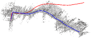
(a) ICP

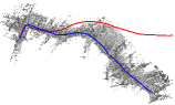
(b) ICP-KP

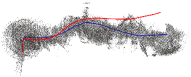
(c) ICP-KN

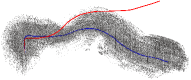
(d) GMM

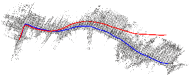
(e) CPD

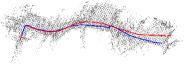
(f) ECM

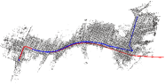
(g) TEASER++

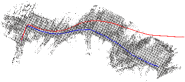
(h) FGR

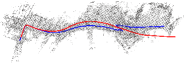
(i) FRICP

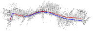
(j) PIPL

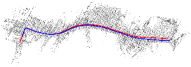
(k) Ours

Figure 15: Registration results of all compared methods on the KITTI 03 sequence odemetry dataset, where red and blue curves indicate the ground truth and the registration result, respectively. The proposed method shows the highest accuracy.

IV-G Registration on ETH TLS Datasets

In this experiment, we evaluate our method on a series of partially overlapping and large-scale ETH terrestrial laser scanner (TLS) datasets [61], which have been broadly used in photogrammetry and remote sensing society. We adopt five-pair point clouds from the Facade dataset for testing, and downsample them by voxel grid filtering with gridStep=0.1 because each point cloud has at least $1.5\times 10^{7}$ points. Fig. 12 presents two test examples. We conduct 10 experiments and report the average performance in Table IV, where green and red are the first two highest accuracy. As observed, our method outperforms competitors with the overall highest precision, followed by FGR and FRICP. The ICP optimized by MATLAB is the fastest, with time consumption around 0.2s. Our algorithm spends about 0.34s on average and is faster than other approaches. TEASER++, FGR, FRICP, and PIPL are also efficient, but their performance is slightly lower than ours in terms of accuracy and efficiency. Probabilistic methods again consume the most time, but compared with ICP-based methods, no noticeable improvement of the registration precision is observed; thus, they are more suitable for sparse and coarse alignments. We present examples in Fig. 13, where values in parentheses are corresponding deviations.

IV-H Registration on KITTI Odometry Datasets

We also assess the stability of the proposed method on the large-scale outdoor KITTI odometry benchmark datasets [1] developed by a velodyne laser scanner. The corresponding ground truth poses are determined by an IMU measurement and an RTK GPS localization system. We adopt the 03 odometry sequence, including 801 point cloud frames for testing, and downsample them by the voxelized grid with gridStep=0.5. First, we register every other consecutive frame among the whole sequences, i.e., $frame_{801}$ to $frame_{799}$, $frame_{799}$ to $frame_{797}$, $frame_{k}$ to $frame_{k-2}~{}(k\geq 3)$, $\cdots$, and $frame_{3}$ to $frame_{1}$, to reconstruct the whole outdoor scene. A total of 401 point cloud pairs are available for registration. Then, we compose these 401 pairwise transformations $\mathcal{T}_{1}$, $\cdots$, $\mathcal{T}_{401}$ to align frames to the first one. For instance, we use $\mathcal{T}_{1}\cdot\mathcal{T}_{2}\cdots\mathcal{T}_{401}(frame_{801})$ to align $frame_{801}$ to $frame_{1}$. Our purpose is to evaluate the performance of the designed algorithm against accumulative deviations. Similar to [62], we evaluate the average errors of the relative and the absolute rotation and translation, as well as the deviation of the last frame with respect to the first one. The translation error is the Euclidean distance between the estimated translation vector and the ground truth value.

The quantitative deviations and registration results are reported in Table V and Fig. 15, respectively. As observed, our proposed method attains the most accurate results in all situations. The compared methods show minor relative errors but suffer from the absolute case, especially for the translation estimation, indicating that they have relatively large accumulative errors among the registration process. However, our method performs more stable, has lower errors for rotation and translation estimation of the absolute case, and achieves more satisfactory registration of the last frame among the whole 401 sequences. Fig. 16 records the specific registration process of all point cloud frames of our method, except for few spikes, all relative errors are small, with values less than 0.4. Therefore, the whole registration is fairly stable. Absolute translation errors slightly increase due to the accumulative deviation. However, our method still outperforms competitors with the highest registration precision, and the errors indeed can be further relieved by requesting additional advanced techniques, such as stereo images or loop-closure detection. We present some intermediate registration results in Fig. 17, where blue ellipses indicate large deviations.

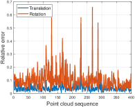
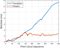
Figure 16: Record of the registration process of the proposed method on 401 point cloud sequences.

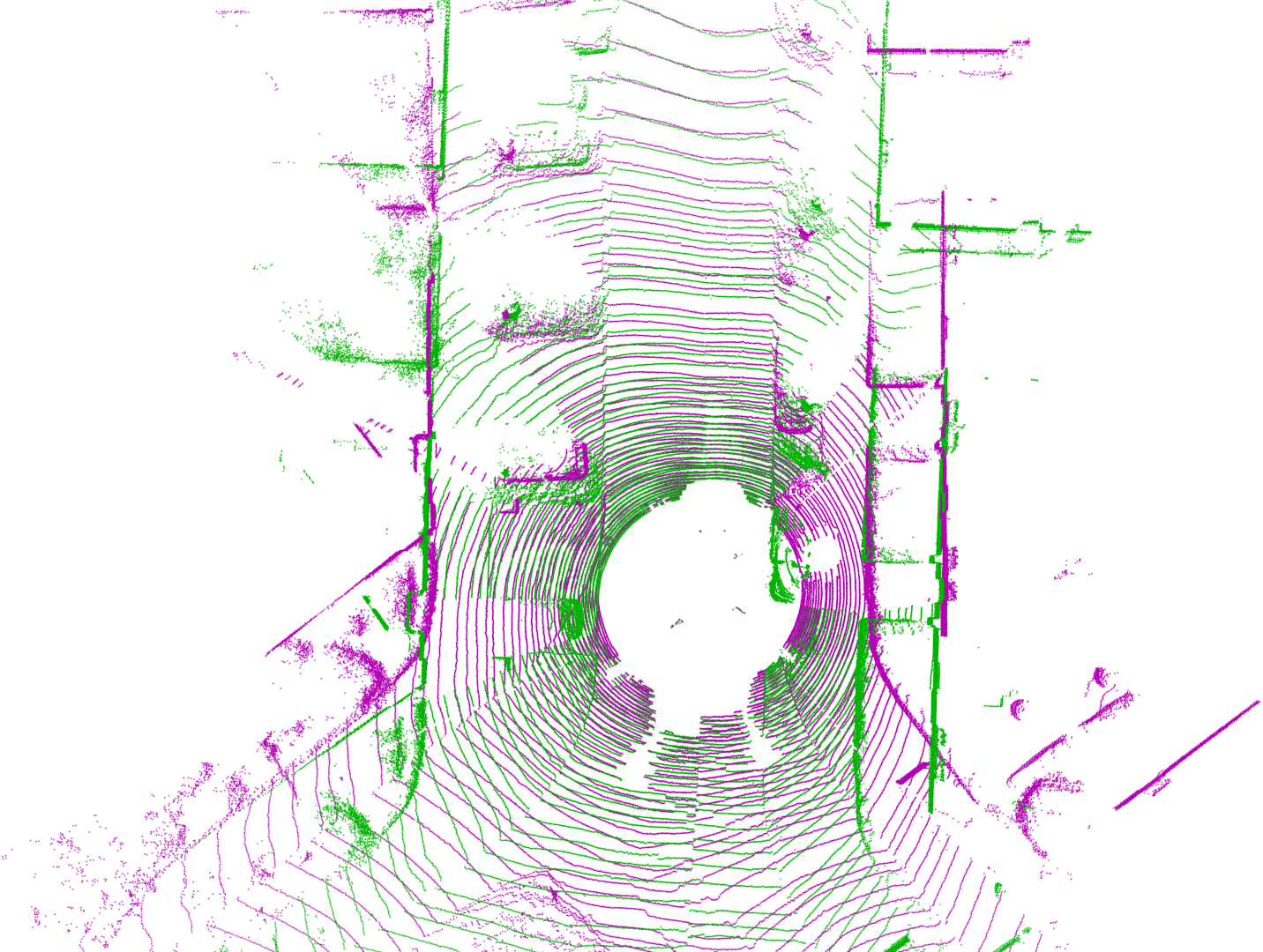
(a) Misalignment

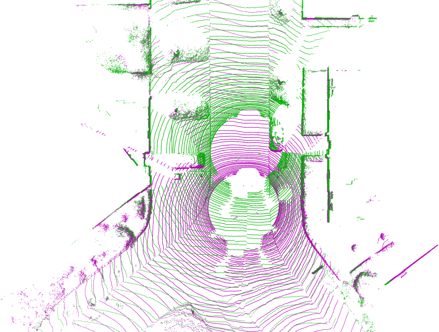
(b) ICP

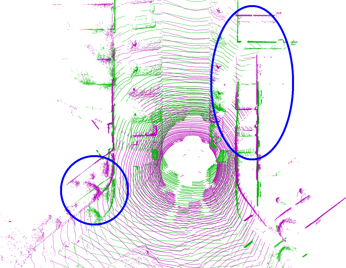
(c) ICP-KP

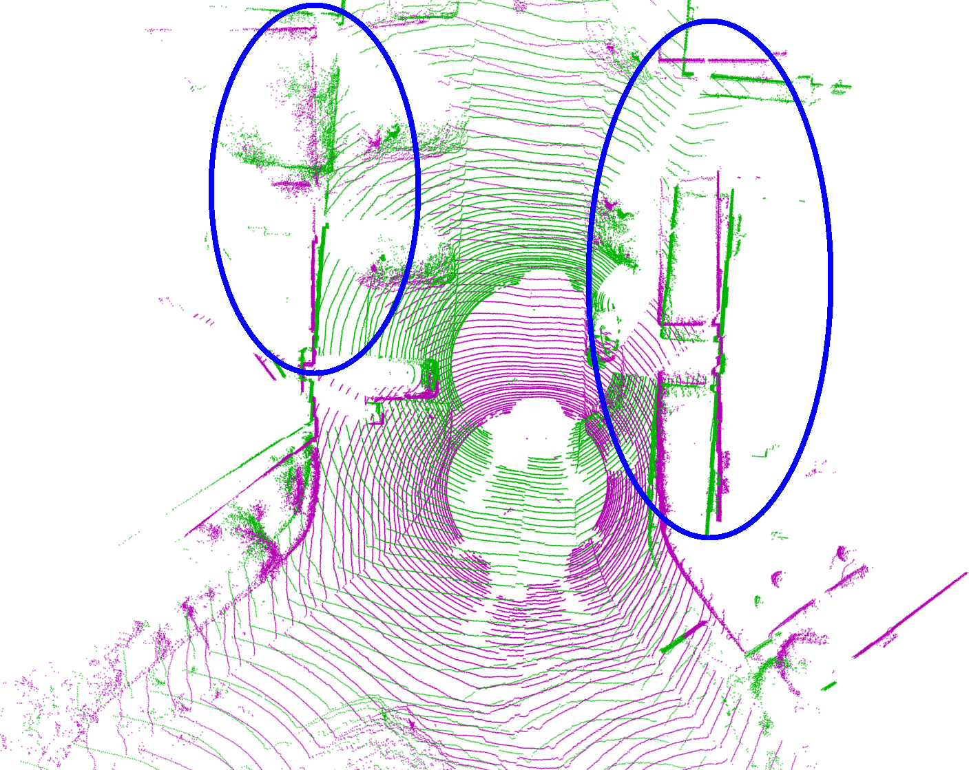
(d) ICP-KN

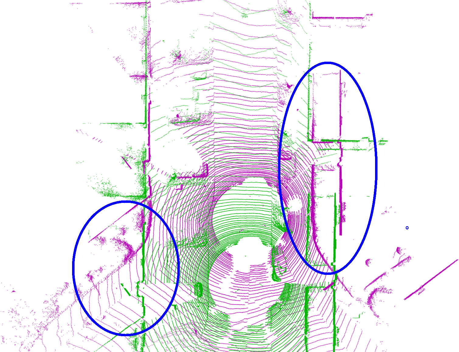
(e) GMM

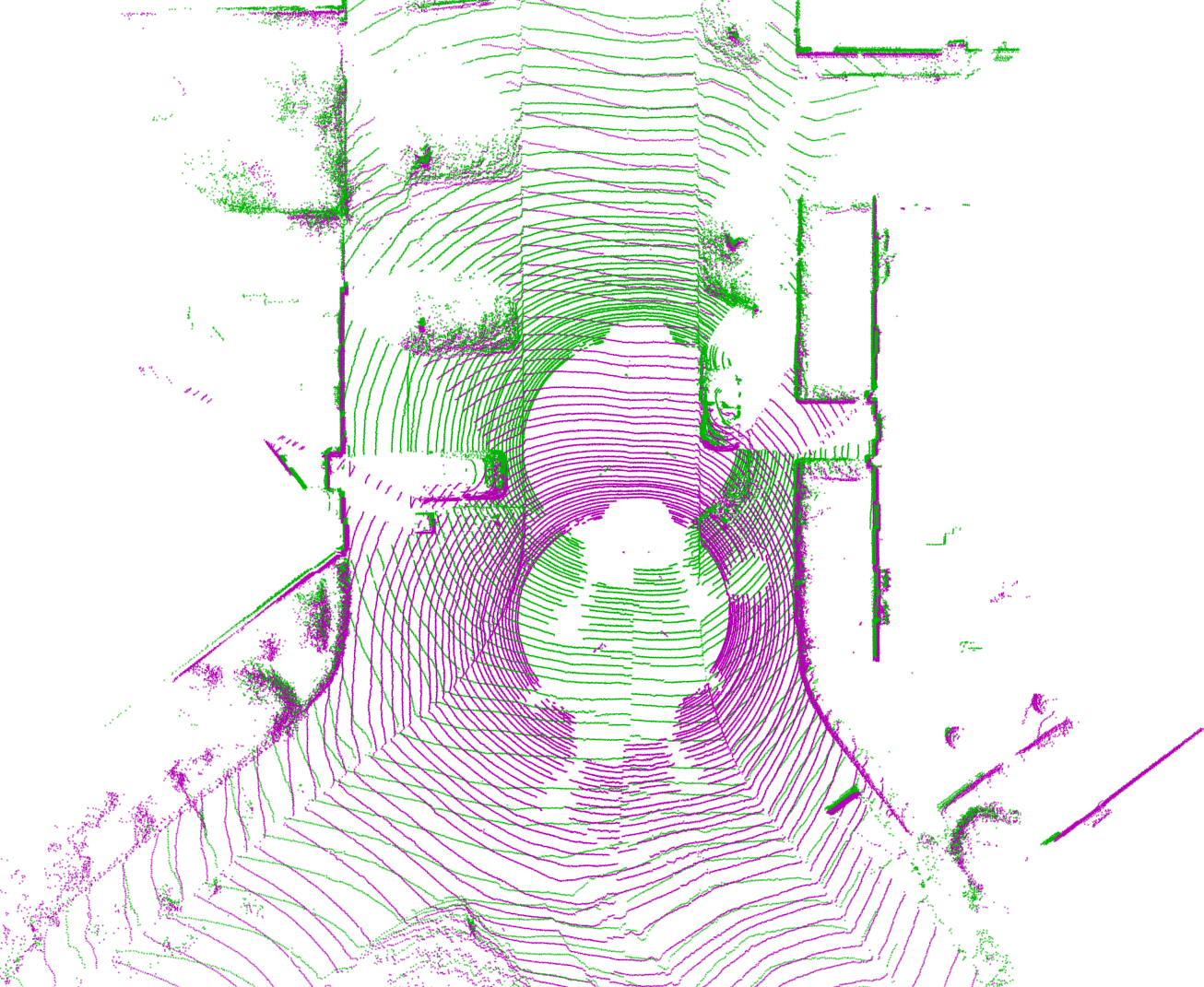
(f) CPD

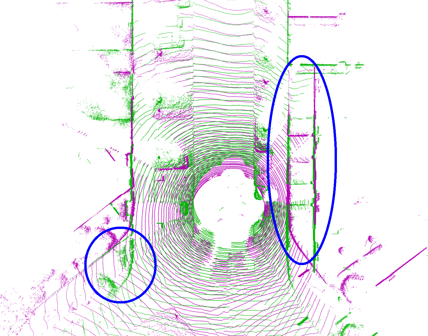
(g) ECM

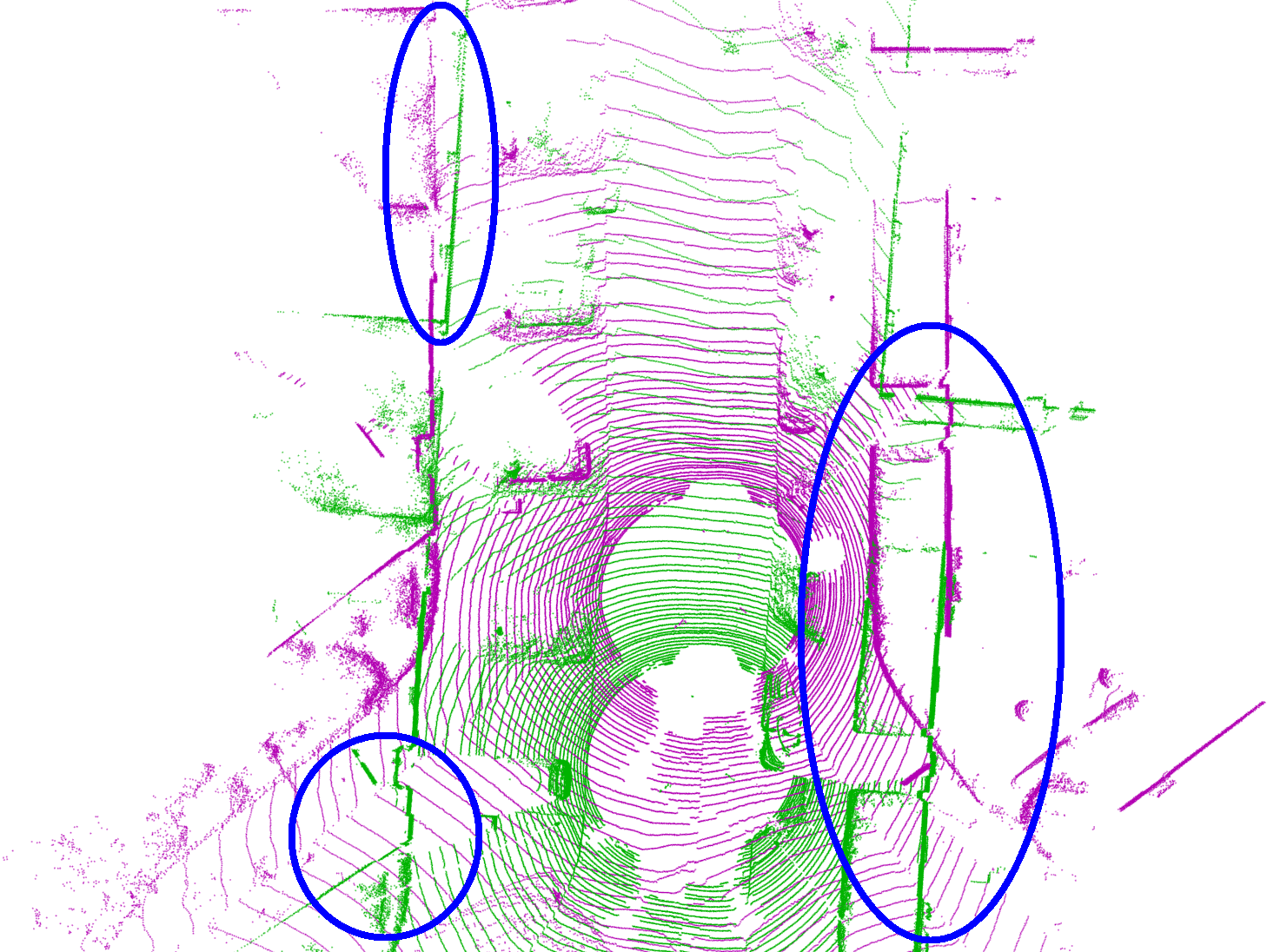
(h) TEASER++

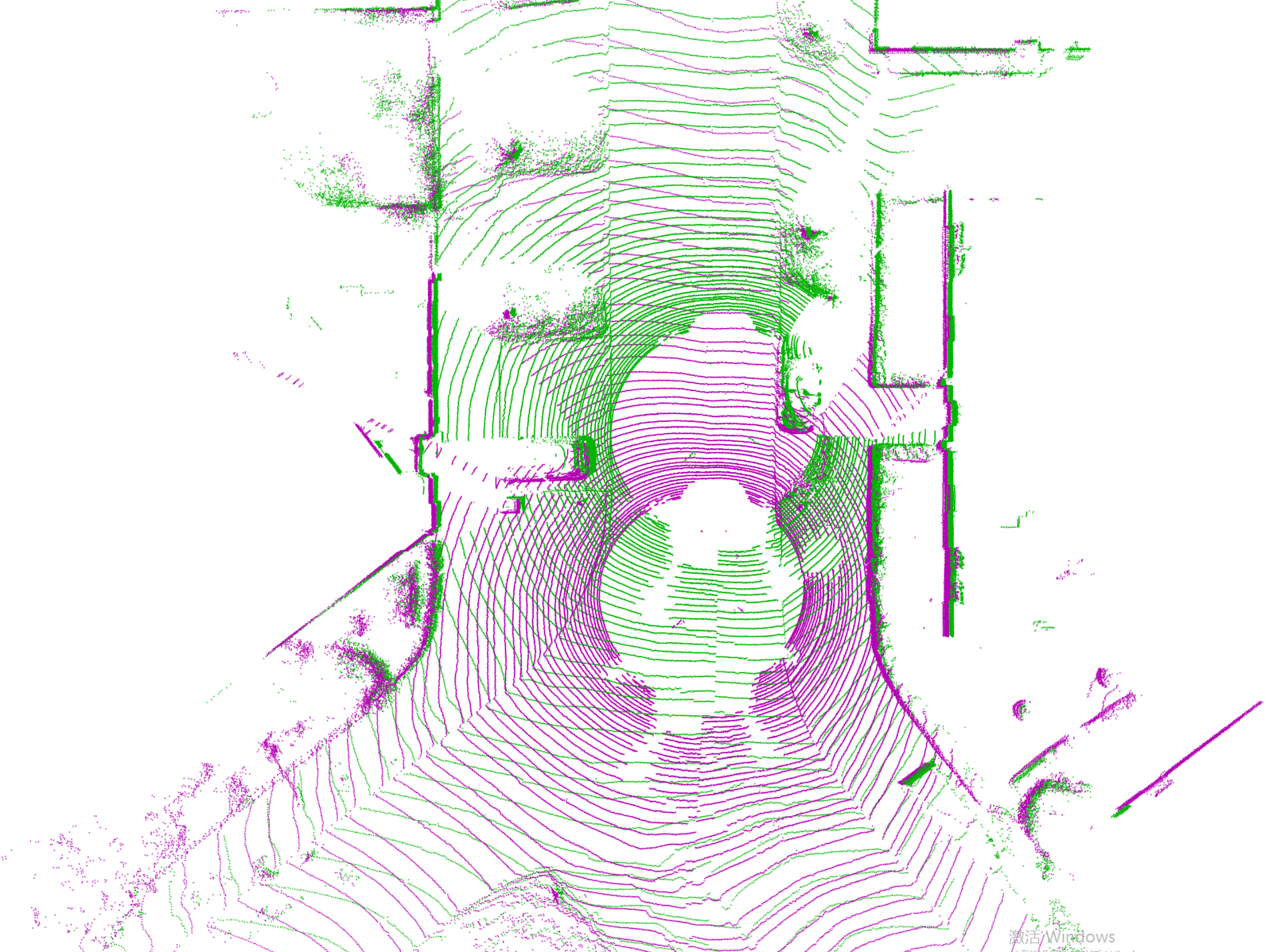
(i) FGR

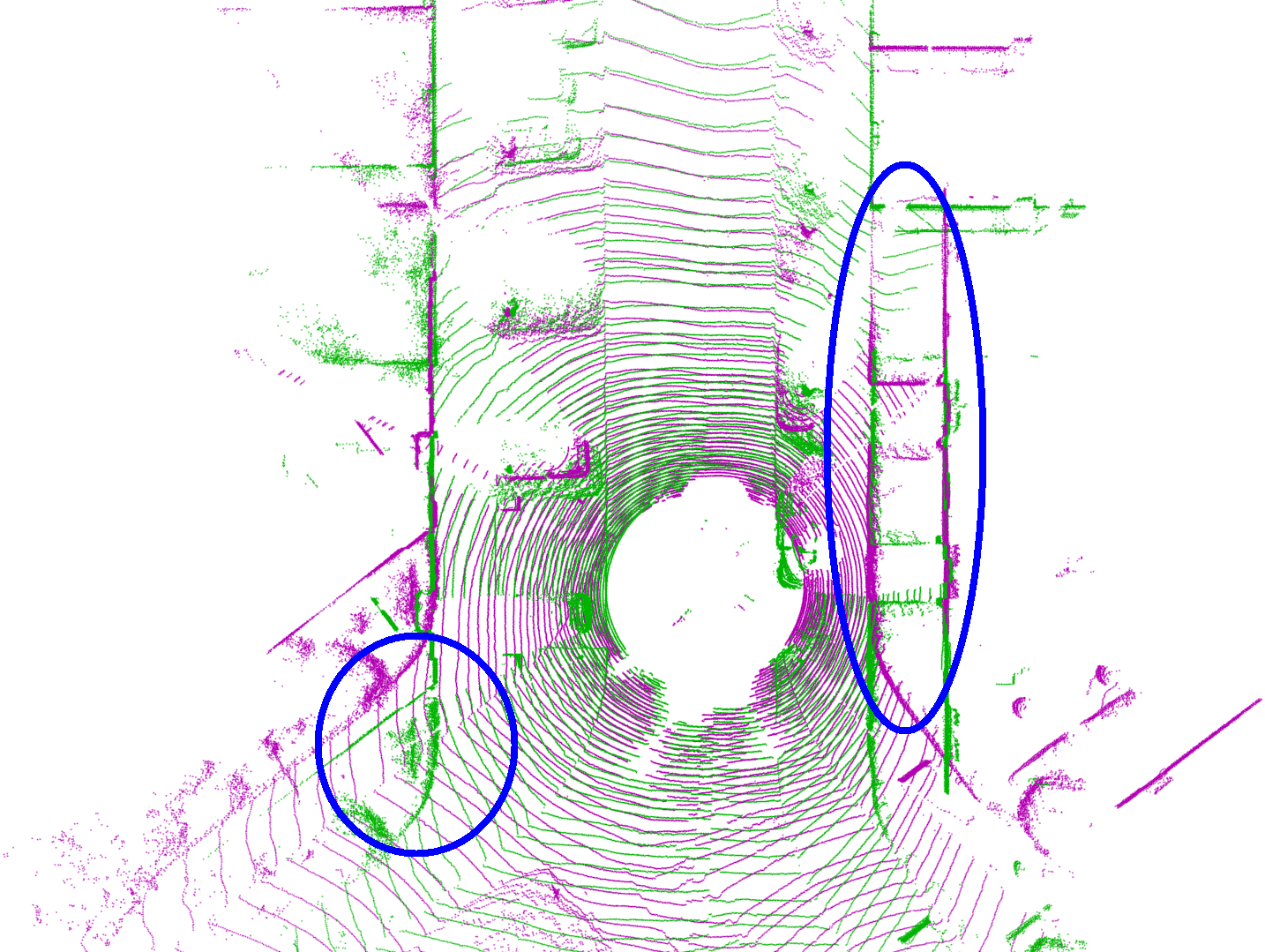
(j) FRICP

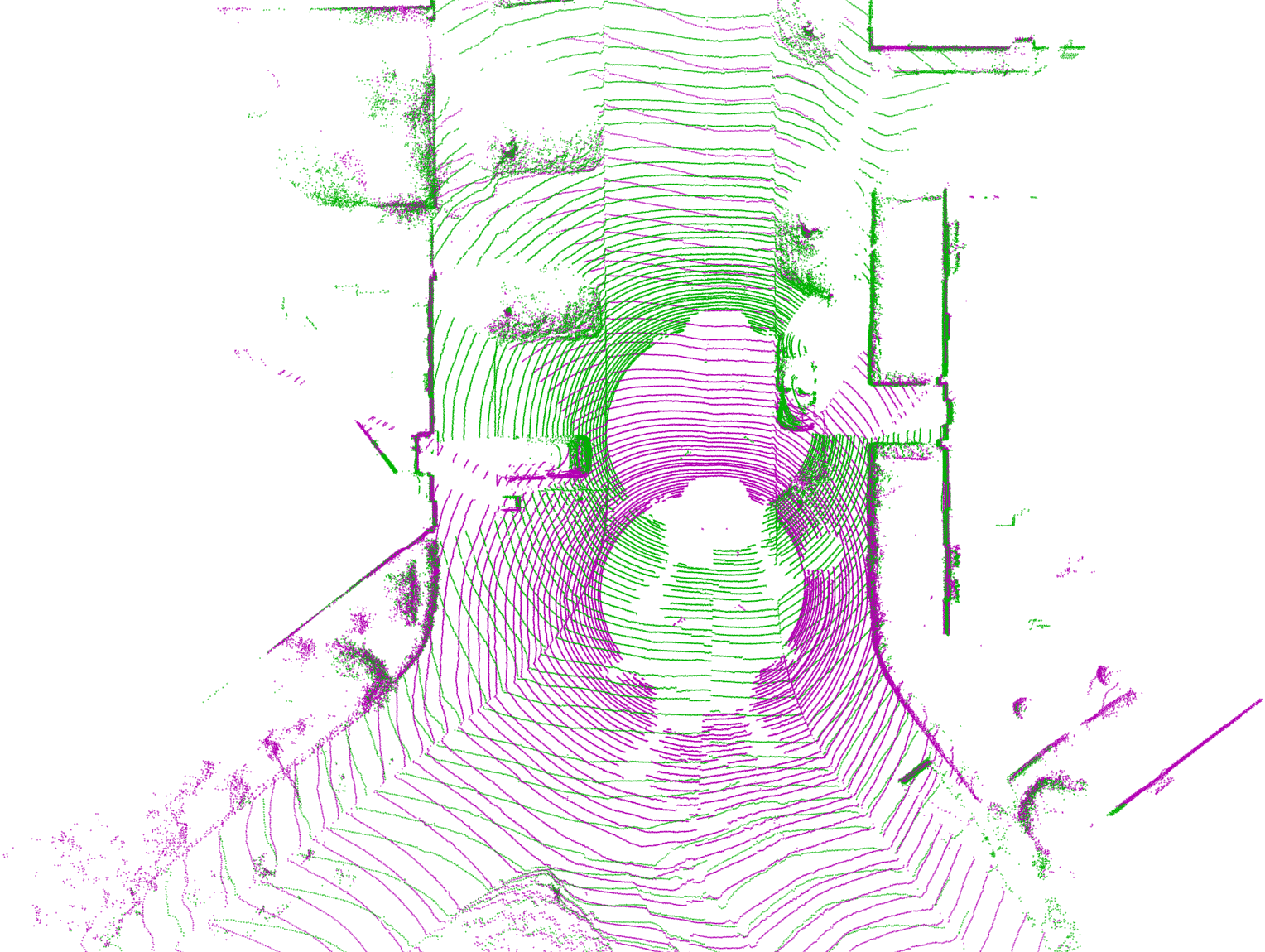
(k) PIPL

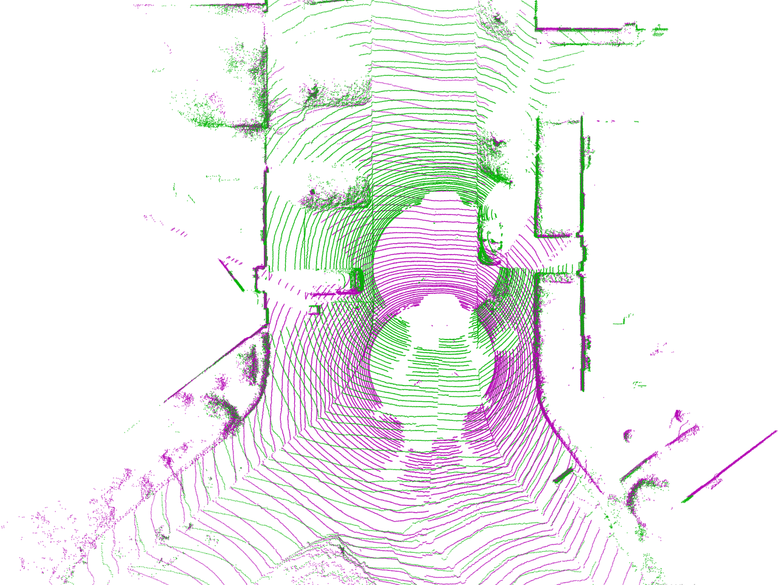
(l) Ours

Figure 17: Qualitative registration results on the KITTI odometry datasets, where blue ellipses indicate significant errors.

(a) *

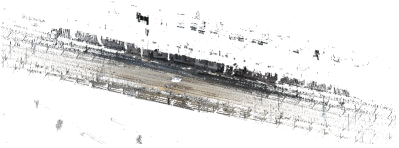
(b) *

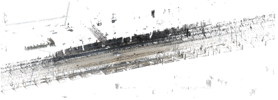
Figure 18: Two pair of scanned real-world railway point clouds endowed with nonuniform point density.

TABLE VI: Quantitative registration results on the WHU-TLS Railway dataset.

	Metric	ICP[2]	ICP-KP[53]	ICP-KN[53]	GMM[6]	CPD[7]	ECM[8]	TEASER++[30]	FGR[28]	FRICP[31]	PIPL[3]	Ours
Railway 1	RMSD	34.4934	40.4979	42.2538	52.0106	47.8289	41.8326	179.2847	42.2166	40.4123	37.9666	22.7206
	AngErr	0.6628	0.6400	3.1715	0.2340	3.7988	0.1641	171.1502	3.7534	0.0799	7.5604	0.1119
Railway 2	RMSD	54.2542	54.3514	67.3334	64.7316	54.6875	50.7399	213.2731	166.4902	40.6263	33.0830	30.5180
	AngErr	2.0299	2.0372	4.7293	0.8820	4.5592	0.1989	73.0722	163.6932	0.1476	9.7713	0.1399

IV-I Robustness against Initial Poses

We also investigate the robustness of the proposed method against initial poses of point clouds. To this end, we rotate the Dragon model along the $X,$ $Y,$ $Z$ axes separately and change its rotation angle from $[-120^{\circ},120^{\circ}]$ with the angle interval equal to $5^{\circ}$. A total of $49\times 3$ point cloud pairs are available for registration. We use the root-mean-squared distance (RMSD) defined as

$$RMSD=\sqrt{\frac{1}{M}\sum_{i=1}^{M}\|\hat{\mathcal{T}}\bm{x}_{i}-{\mathcal{T}}\bm{x}_{i}\|_{2}^{2}}$$ (20)

to assess the registration performance, where $\hat{\mathcal{T}}$ and ${\mathcal{T}}$ are the solved and ground truth transformation, respectively. Fig. 19 shows the registration results against rotation angles. ICP is involved here as an indicator to the sensitivity of the initial poses. For all cases, the proposed method has wider angle range for correct registration than the baseline PIPL and is much larger than ICP. Even for the first case where ICP requires strict initialization, our method still tolerates nearly $45^{\circ}$ rotation angle, suggesting its high robustness against initial poses and the conservation of efforts for initialization tuning.

IV-J Influence of Nonuniform Point Density

We further perform experiments to investigate the influence of nonuniform point density for point cloud registration. As presented in Fig. 18, we use two pairs of scanned outdoor point clouds named Railway 1 and Railway 2 from the WHU-TLS dataset [63] for testing. As observed, these point clouds have nonuniform point density, and their central parts are much denser than both ends. The registration results regarding RMSD and AngErr are reported in Table VI. Except for TEASER++ and FGR which generate significant AngErr, the other approaches attain acceptable AngErr. Moreover, FRICP and our method have the most accurate rotation estimation. Meanwhile, our algorithm also outperforms competitors with the lowest RMSD, indicating that it is more robust and stable against nonuniform point clouds. Considering space limitation, we present the registration results of each method in Supplemental Material.

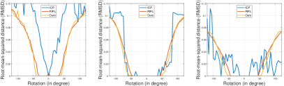
Figure 19: Robustness test against initial poses. From left to right are the registration results by rotating point clouds along the $X,$ $Y,$ and $Z$ axes.

IV-K Investigation of the $X84$ Principle

We also investigate the choice of $\alpha$ in the $X84$ principle, i.e., $\mathcal{I}(\bm{x}_{i})>\alpha\cdot\text{MAD}(\mathcal{I}(\mathbf{X}))$, for the influence of robustness against outliers. We contaminate the two Bunny models (000, 045) [45] with a set of outliers sampled from either Gaussian or uniform distribution. The Gaussian distribution is with zero mean, and its standard variance along $X,Y,Z$ is separately equal to the size of the three sides of the point cloud bounding box, whereas the uniform distribution is directly built on the basis of the point cloud bounding box. For instance, Fig. 20(a) and (b) give two test samples with 50% Gaussian outliers and 80% uniform outliers, respectively. We increase the outlier ratio from 10% to 80% and vary $\alpha=5.2$ to $\alpha=8.0$ for both Gaussian and uniform outliers to assess the $X84$ principle. Results in Fig. 20(c) suggest that under Gaussian outlier contamination, $k=5.2$ has the breakdown point up to $50\%$, whereas $k=8.0$ only tolerates $30\%$ of the outliers. As for uniform outliers, $k=5.2$ and $k=8.0$ attain highly robust performance. Therefore, the $X84$ principle is credible, and $k=5.2$ is suggested for practical use, especially without a priori information of the outlier type. Registration results of Fig. 20(a) and (b) by our method (with $k=5.2$) are reported in Fig. 20(d) and (e), respectively.

(a) Gaussian

(b) Uniform

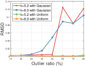
(c) RMSD

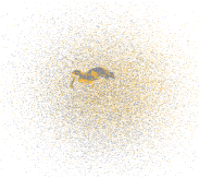
(d) RMSD=0.0035 ($k=5.2$)

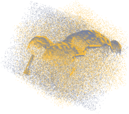
(e) RMSD=0.0032 ($k=5.2$)

Figure 20: Investigation of the $X84$ principle for outlier depression. $k=5.2$ gives high robustness and is suggested for practical use especially when the outlier type is unknown.

V Discussion and Conclusions

We presented a precise and efficient pipeline for robust point cloud registration in various 3D scenes from range scanners to LiDAR. Our first contribution is exploiting GSP to describe the local surface variation, from which we define the point response intensity and theoretically prove its invariance under rigid transformations. Together, the point response intensity combined with median absolute deviation in robust statistics successfully removes most noisy outliers, resulting in more stable and accurate registration. Moreover, we take point response intensity as a metric to assess the particle mass, which naturally reflects the position distribution importance. We also embed higher-order features, such as surface normals and curvatures, in GSP to create a novel geometric invariant under rigid transformations, thereby enabling credible correspondence among point pairs, boosting the modeling of forces, and discerning of different particles. Finally, we introduce the adaptive simulated annealing framework for high-efficiency solving of the global optimal transformation. Our method improves the physics-based point cloud registration framework regarding accuracy, robustness, and efficiency.

Extensive experiments on a wide variety of datasets confirm the accuracy, efficiency, and robustness of our proposed method, indicating its promising performance for processing large-scale scans. Given the convenient feature representation mechanism, GSP-induced invariants can be generalized to ICP-based and probabilistic-based registration, reducing their computational complexity and enhancing the point matching confidence. The currently proposed method is limited to the rigid transformation without scaling and pays minimal attention on robust loss functions. Future work will seek for scale-invariant graph filters that can further enrich the geometric feature description, which will be conducive to cross-modal registration, where scale difference commonly exists, e.g., the point clouds captured by Kinect cameras and laser scanners. We also plan to invoke M/S-estimators, adaptive influence function, or robust $L_{p}$ minimization to current work to improve its robustness further. Finally, in a future study, the rigid framework can be extended to non-rigid registration by modeling forces via fluid/elastic mechanics, and continuous time series through integral can be used to analyze the complex deformable process.

References

- [1] A. Geiger, P. Lenz, and R. Urtasun, “Are we ready for autonomous driving? the KITTI vision benchmark suite,” in Proc. IEEE Conf. Comput. Vis. Pattern Recog., Providence, RI, USA, 2012, pp. 3354–3361.
- [2] P. Besl and N. D. McKay, “A method for registration of 3-d shapes,” IEEE Trans. Pattern Anal. Mach. Intell., vol. 14, no. 2, pp. 239–256, Feb. 1992.
- [3] P. Jauer, I. Kuhlemann, R. Bruder, A. Schweikard, and F. Ernst, “Efficient registration of high-resolution feature enhanced point clouds,” IEEE Trans. Pattern Anal. Mach. Intell., vol. 41, no. 5, pp. 1102–1115, May 2018.
- [4] W. Gao and R. Tedrake, “Filterreg: Robust and efficient probabilistic point-set registration using Gaussian filter and twist parameterization,” in Proc. IEEE Conf. Comput. Vis. Pattern Recog., Long Beach, CA, USA, 2019, pp. 11 095–11 104.
- [5] P. Song, “Local voxelizer: A shape descriptor for surface registration,” Comput. Vis. Media, vol. 1, no. 4, pp. 279–289, Oct. 2015.
- [6] B. Jian and B. C. Vemuri, “Robust point set registration using Gaussian mixture models,” IEEE Trans. Pattern Anal. Mach. Intell., vol. 33, no. 8, pp. 1633–1645, Aug. 2010.
- [7] A. Myronenko and X. Song, “Point set registration: Coherent point drift,” IEEE Trans. Pattern Anal. Mach. Intell., vol. 32, no. 12, pp. 2262–2275, Dec. 2010.
- [8] R. Horaud, F. Forbes, M. Yguel, G. Dewaele, and J. Zhang, “Rigid and articulated point registration with expectation conditional maximization,” IEEE Trans. Pattern Anal. Mach. Intell., vol. 33, no. 3, pp. 587–602, March 2010.
- [9] P. Biber and W. Straßer, “The normal distributions transform: A new approach to laser scan matching,” in IEEE/RSJ Int. Conf. Intell. Robot. Syst., vol. 3, Las Vegas, NV, USA, 2003, pp. 2743–2748.
- [10] Y. Tsin and T. Kanade, “A correlation-based approach to robust point set registration,” in Proc. Eur. Conf. Comput. Vis., 2004, pp. 558–569.
- [11] V. Golyanik, S. A. Ali, and D. Stricker, “Gravitational approach for point set registration,” in Proc. IEEE Conf. Comput. Vis. Pattern Recog., Las Vegas, NV, USA, 2016, pp. 5802–5810.
- [12] V. Golyanik, C. Theobalt, and D. Stricker, “Accelerated gravitational point set alignment with altered physical laws,” in Proc. IEEE Int. Conf. Comput. Vis., Seoul, Korea (South), 2019, pp. 2080–2089.
- [13] A. Ortega, P. Frossard, J. Kovačević, J. M. Moura, and P. Vandergheynst, “Graph signal processing: Overview, challenges, and applications,” Proc. IEEE, vol. 106, no. 5, pp. 808–828, May 2018.
- [14] C. Deng, X. Yang, F. Nie, and D. Tao, “Saliency detection via a multiple self-weighted graph-based manifold ranking,” IEEE Trans. Multimedia, vol. 22, no. 4, pp. 885–896, April 2019.
- [15] J. Zeng, G. Cheung, M. Ng, J. Pang, and C. Yang, “3D point cloud denoising using graph laplacian regularization of a low dimensional manifold model,” IEEE Trans. Image Process., vol. 29, pp. 3474–3489, Dec. 2019.
- [16] A. Sakiyama, Y. Tanaka, T. Tanaka, and A. Ortega, “Eigendecomposition-free sampling set selection for graph signals,” IEEE Trans. Signal Process., vol. 67, no. 10, pp. 2679–2692, May 2019.
- [17] A. Sandryhaila and J. M. Moura, “Discrete signal processing on graphs,” IEEE Trans. Signal Process., vol. 61, no. 7, pp. 1644–1656, April 2013.
- [18] ——, “Big data analysis with signal processing on graphs: Representation and processing of massive data sets with irregular structure,” IEEE Signal Proc. Mag., vol. 31, no. 5, pp. 80–90, Sept. 2014.
- [19] F. Pomerleau, F. Colas, and R. Siegwart, “A review of point cloud registration algorithms for mobile robotics,” Found. Trends. Robot., vol. 4, no. 1, pp. 1–104, May 2015.
- [20] Y. Chen and G. Medioni, “Object modelling by registration of multiple range images,” Image Vision Comput, vol. 10, no. 3, pp. 145–155, April 1992.
- [21] J. Park, Q.-Y. Zhou, and V. Koltun, “Colored point cloud registration revisited,” in Proc. IEEE Int. Conf. Comput. Vis., Venice, Italy, 2017, pp. 143–152.
- [22] D. Aiger, N. J. Mitra, and D. Cohen-Or, “4-points congruent sets for robust pairwise surface registration,” in ACM SIGGRAPH 2008 papers, 2008, pp. 1–10.
- [23] N. Mellado, D. Aiger, and N. J. Mitra, “Super 4PCS fast global pointcloud registration via smart indexing,” in Comput. Graph. Forum, vol. 33, no. 5, Aug. 2014, pp. 205–215.
- [24] J. Yang, H. Li, and Y. Jia, “Go-ICP: Solving 3D registration efficiently and globally optimally,” in Proc. IEEE Int. Conf. Comput. Vis., Sydney, NSW, Australia, 2013, pp. 1457–1464.
- [25] Z. Dong, F. Liang, B. Yang, Y. Xu, Y. Zang, J. Li, Y. Wang, W. Dai, H. Fan, J. Hyyppä et al., “Registration of large-scale terrestrial laser scanner point clouds: A review and benchmark,” ISPRS J. PhotoGramm., vol. 163, pp. 327–342, May 2020.
- [26] D. Chetverikov, D. Svirko, D. Stepanov, and P. Krsek, “The Trimmed iterative closest point algorithm,” in Int. Conf. Pattern Recog., vol. 3, Quebec City, QC, Canada, 2002, pp. 545–548 vol.3.
- [27] S. Bouaziz, A. Tagliasacchi, and M. Pauly, “Sparse iterative closest point,” in Comput. Graph. Forum, vol. 32, no. 5, Aug. 2013, pp. 113–123.
- [28] Q.-Y. Zhou, J. Park, and V. Koltun, “Fast global registration,” in Proc. Eur. Conf. Comput. Vis., 2016, pp. 766–782.
- [29] R. B. Rusu, N. Blodow, and M. Beetz, “Fast point feature histograms (FPFH) for 3D registration,” in IEEE Int. Conf. Robot. Autom., Kobe, Japan, 2009, pp. 3212–3217.
- [30] H. Yang, J. Shi, and L. Carlone, “TEASER: Fast and certifiable point cloud registration,” IEEE Trans. Robot., vol. 37, no. 2, pp. 314–333, April 2021.
- [31] J. Zhang, Y. Yao, and B. Deng, “Fast and robust iterative closest point,” IEEE Trans. Pattern Anal. Mach. Intell., vol. 44, no. 7, pp. 3450–3466, July 2021.
- [32] Y. Aoki, H. Goforth, R. A. Srivatsan, and S. Lucey, “Pointnetlk: Robust & efficient point cloud registration using pointnet,” in Proc. IEEE Conf. Comput. Vis. Pattern Recog., Long Beach, CA, USA, 2019, pp. 7163–7172.
- [33] C. R. Qi, H. Su, K. Mo, and L. J. Guibas, “Pointnet: Deep learning on point sets for 3D classification and segmentation,” in Proc. IEEE Conf. Comput. Vis. Pattern Recog., Honolulu, HI, USA, 2017, pp. 652–660.
- [34] Y. Wang and J. M. Solomon, “Deep closest point: Learning representations for point cloud registration,” in Proc. IEEE Int. Conf. Comput. Vis., Seoul, Korea (South), 2019, pp. 3523–3532.
- [35] C. Choy, W. Dong, and V. Koltun, “Deep global registration,” in Proc. IEEE Conf. Comput. Vis. Pattern Recog., Seattle, WA, USA, 2020, pp. 2514–2523.
- [36] D. I. Shuman, S. K. Narang, P. Frossard, A. Ortega, and P. Vandergheynst, “The emerging field of signal processing on graphs: Extending high-dimensional data analysis to networks and other irregular domains,” IEEE Signal Proc. Mag., vol. 30, no. 3, pp. 83–98, May 2013.
- [37] S. Zhang, S. Cui, and Z. Ding, “Hypergraph spectral analysis and processing in 3d point cloud,” IEEE Trans. Image Process., vol. 30, pp. 1193–1206, Dec. 2020.
- [38] C. Dinesh, G. Cheung, and I. V. Bajić, “Point cloud denoising via feature graph Laplacian regularization,” IEEE Trans. Image Process., vol. 29, pp. 4143–4158, Jan. 2020.
- [39] S. Chen, D. Tian, C. Feng, A. Vetro, and J. Kovačević, “Fast resampling of three-dimensional point clouds via graphs,” IEEE Trans. Signal Process., vol. 66, no. 3, pp. 666–681, Feb. 2017.
- [40] Q. Deng, S. Zhang, and Z. Ding, “An efficient hypergraph approach to robust point cloud resampling,” IEEE Trans. Image Process., vol. 31, pp. 1924–1937, Feb. 2022.
- [41] D. Cohen-Or, C. Greif, T. Ju, N. J. Mitra, A. Shamir, O. Sorkine-Hornung, and H. R. Zhang, A sampler of useful computational tools for applied geometry, computer graphics, and image processing, 2015.
- [42] F. R. Hampel, E. M. Ronchetti, P. J. Rousseeuw, and W. A. Stahel, Robust statistics: the approach based on influence functions. John Wiley & Sons, 2011, vol. 196.
- [43] “Point Cloud Subjective Assessment Database. [Online]. Available,” https://vision.nju.edu.cn.
- [44] R. M. Dreizler and C. S. Lüdde, Theoretical Mechanics: Theoretical Physics 1, 2010.
- [45] “The Stanford 3D Scanning Repository. [Online]. Available,” http://graphics.stanford.edu/data/3Dscanrep/.
- [46] C. Tomasi, “Vector representation of rotations,” Comput. Sci., vol. 527, 2013.
- [47] K. Kanatani, Understanding geometric algebra: Hamilton, Grassmann, and Clifford for computer vision and graphics, 2015.
- [48] J. Kovacs, “Coulomb’s law,” Michigan State University, 2001.
- [49] J. L. Bentley, “Multidimensional binary search trees used for associative searching,” Commun. ACM, vol. 18, no. 9, pp. 509–517, Sept. 1975.
- [50] J. H. Friedman, The elements of statistical learning: Data mining, inference, and prediction, 2017.
- [51] V. A. Cicirello, “On the design of an adaptive simulated annealing algorithm,” in Proc. Int. Conf. Princ. Pract. Constr. Program. AAAI Press, 2007.
- [52] L. Ingber, “Adaptive simulated annealing (ASA): Lessons learned.”
- [53] H. M. Kjer and J. Wilm, “Evaluation of surface registration algorithms for pet motion correction,” B.S. thesis, 2010.
- [54] H. Hoppe, T. DeRose, T. Duchamp, J. McDonald, and W. Stuetzle, “Surface reconstruction from unorganized points,” in Proc. Annu. Conf. Comput. Graph. Interact. Tech., 1992, pp. 71–78.
- [55] O. Hirose, “A bayesian formulation of coherent point drift,” IEEE Trans. Pattern Anal. Mach. Intell., vol. 43, no. 7, pp. 2269–2286, July 2021.
- [56] “Statue Model Repository. [Online]. Available,” https://lgg.epfl.ch/statues_dataset.php.
- [57] “Open3D Library, [Online]. Available,” http://www.open3d.org/.
- [58] A. S. Mian, M. Bennamoun, and R. Owens, “Three-dimensional model-based object recognition and segmentation in cluttered scenes,” IEEE Trans. Pattern Anal. Mach. Intell., vol. 28, no. 10, pp. 1584–1601, Oct. 2006.
- [59] “Large Geometric Models Archive. [Online]. Available,” https://www.cc.gatech.edu/projects/large_models/.
- [60] “OpenGR Library, [Online]. Available,” https://github.com/STORM-IRIT/OpenGR/.
- [61] “Terrestrial Laser Scanner Point Clouds. [Online]. Available,” https://prs.igp.ethz.ch/research/completed_projects.html.
- [62] W. Liu, H. Wu, and G. S. Chirikjian, “LSG-CPD: Coherent point drift with local surface geometry for point cloud registration,” in Proc. IEEE Int. Conf. Comput. Vis., Montreal, QC, Canada, 2021, pp. 15 273–15 282.
- [63] Z. Dong, B. Yang, Y. Liu, F. Liang, B. Li, and Y. Zang, “A novel binary shape context for 3d local surface description,” ISPRS J. PhotoGramm., vol. 130, pp. 431–452, Aug. 2017.