New Linear-time Algorithm for SubTree Kernel Computation based on Root-Weighted Tree Automata

Abstract

Tree kernels have been proposed to be used in many areas as the automatic learning of natural language applications. In this paper, we propose a new linear time algorithm based on the concept of weighted tree automata for SubTree kernel computation. First, we introduce a new class of weighted tree automata, called Root-Weighted Tree Automata, and their associated formal tree series. Then we define, from this class, the SubTree automata that represent compact computational models for finite tree languages. This allows us to design a theoretically guaranteed linear-time algorithm for computing the SubTree Kernel based on weighted tree automata intersection. The key idea behind the proposed algorithm is to replace DAG reduction and nodes sorting steps used in previous approaches by states equivalence classes computation allowed in the weighted tree automata approach. Our approach has three major advantages: it is output-sensitive, it is free sensitive from the tree types (ordered trees versus unordered trees), and it is well adapted to any incremental tree kernel based learning methods. Finally, we conduct a variety of comparative experiments on a wide range of synthetic tree languages datasets adapted for a deep algorithm analysis. The obtained results show that the proposed algorithm outperforms state-of-the-art methods.

1 Introduction

Kernel methods have been widely used to extend the applicability of many well-known algorithms, such as the Perceptron [1], Support Vector Machines [2], or Principal Component Analysis [3]. Tree kernels are interesting approaches in areas of machine learning based natural language processing. They have been applied to reduce such effort for several natural language tasks, e.g., relation extraction [4], syntactic parsing re-ranking [5], named entity recognition[6, 7], Semantic Role Labeling [8], paraphrase detection [9] and computational argumentation [10].

In [11], Haussler introduces a framework based on convolution kernel to measure the similarity between structured objects in terms of the similarities of their subparts. Based on this idea, many convolution kernels for trees are introduced and have been successfully applied to a variety of problems.

The first proposed kernels in the context of tree structured data were the subtree (ST) kernel [12] and the subset tree (SST) kernel [5]. The first defines a feature space consisting of the set of all proper subtrees, while the second extends this set by also considering subset trees. The research on kernel for trees has evolved either by finding more expressive kernel functions or faster kernels. Expressivity and sparsity has been dealt by introducing ST-like substructures as features: the partial tree (PT) kernel [13] and the elastic tree kernel [14], SubPath [15]. For more details about kernels for trees, we recommend the thesis of Da San Martino 2009 [16].
In this article, we focus on the computation of the ST kernel. The main idea of the ST kernel as introduced in [12] is to compute the number of common subtrees between two trees $t_{1}$ and $t_{2}$ having respectively $m$ and $n$ nodes. It can be recursively computed as follows:

$$K(t_{1},t_{2})=\sum\limits_{(n_{1},n_{2})\in N_{t_{1}}\times N_{t_{2}}}\Delta(n_{1},n_{2})$$ (1)

where $N_{t_{1}}$ and $N_{t_{2}}$ are the set of nodes respectively in $t_{1}$ and $t_{2}$, $\Delta(n_{1},n_{2})=\sum_{i=1}^{|{\cal S}|}I_{i}(n_{1})\cdot I_{i}(n_{2})$ for some finite set of subtrees $S=\{s_{1},s_{2},\cdots\}$, and $I_{i}(n)$ is an indicator function which is equal to $1$ if the subtree is rooted at node $n$ and to $0$ otherwise. Then, a string matching algorithm is used where trees are transformed into strings (see [12] for details). This algorithm has an overall computational complexity equals to $O(\max(m,n)\log(\max(m,n)))$ which is the best worst-case time complexity for this problem.

In [17], Moschitti defined an algorithm for the computation of this type of tree kernels which computes the kernels between two syntactic parse trees in $O(m\times n)$ time, where $m$ and $n$ are the number of nodes in the two trees. Thus, Moschitti modified the equation (1) by introducing a parameter $\sigma\in\{0,1\}$ which enables the SubTrees ($\sigma=1$) or the SubSet Trees ($\sigma=0$) evaluation and which is defined for two trees $t_{1}$ and $t_{2}$ as follows: if the productions at $n_{1}$ and $n_{2}$ are different, then $\Delta(n_{1},n_{2})=0$; if they are the same and $n_{1}$ and $n_{2}$ are leaves, then $\Delta(n_{1},n_{2})=1$; finally if the productions at $n_{1}$ and $n_{2}$ are the same, and if $n_{1}$ and $n_{2}$ are not leaves then $\Delta(n_{1},n_{2})=\prod_{j=1}^{nc(n_{1})}(\sigma+\Delta(C_{n_{1}}^{j},C_{n_{2}}^{j}))$, where $nc(n_{1})$ is the number of children of $n_{1}$ and $C_{n}^{j}$ is $j^{th}$ child of the node $n$. This algorithm can be tuned to avoid any evaluation when $\Delta(n_{1},n_{2})=0$ by efficiently building a node pair set $N_{p}=\{(n_{1},n_{2})\in N_{t_{1}}\times N_{t_{2}}:p(n_{1})=p(n_{2})\}$, where $p(n)$ returns the production rule associated with $n$. It requires the sorting of trees productions at a pre-processing step and then compute $\Delta$ by a dynamic programming approach. This method has a worst-case time complexity in $O(m\times n)$ but in practical applications it provides a quite relevant speed-up.

In 2020, Azais and Ingel [18] develop a unified framework based on Direct Acyclic Graphs (DAG) reduction for computing the ST kernel from ordered or unordered trees, with or without labels on their vertices. DAG reduction of a tree forest is introduced as compact representation of common subtrees structures that makes possible fast computations of the subtree kernel. The main advantage of this approach compared to those based on string representations used by Vishwanathan and Smola, in 2002 is that it makes possible fast repeated computations of the ST kernel. Their method allows the implementation of any weighting function, while the recursive computation of the ST kernel proposed by Aiolli et al. [19] also uses DAG reduction of tree data but makes an extensive use of the exponential form of the weight. They investigate the theoretical complexities of the different steps of the DAG computation and prove that it is in $O(\max(m,n))$ for ordered trees and in $O(\max(m,n)\log(\max(m,n))$ for unordered trees (Proposition 7, [18]).

In the following, we propose a new method to compute the ST kernel using weighted tree automata. We begin by defining a new class of weighted tree automata that we call Rooted Weighted Tree Automata (RWTA). This class of weighted tree automata represents a new efficient and optimal alternative for representing tree forest instead of annotated DAG representation. Then we prove that the ST kernel can be computed efficiently in linear time using a general intersection of RWTA that can be turned into a determinization of a WTA by states accessibility.

The paper is organized as follows: Section LABEL:sec_prel outlines finite tree automata over ranked and unranked trees and regular tree languages. Next, in Section 2, we define a new class of weighted tree automata that we call Rooted Weighted Tree Automata. Thus, in Section 3, the definitions of SubTree series and automata are obtained. Afterwards, in Section 4, we present our algorithms. The first one constructs the RWTA $A_{L}$ as a compact representation of a finite tree language $L$ in linear time. The second one computes the RWTA $A_{X}\odot A_{Y}$ representing the Hadamard product of the RWTAs $A_{X}$ and $A_{Y}$ in time $O(|SubTree(X)|+|SubTree(Y)|)$. Section 5 shows the efficiency of our method by conducting extensive comparative experiments on a variety of tree languages classes. Section 6 concludes the paper.

2 Root-Weighted Tree Automata

Let $\Sigma$ be an alphabet. A tree $t$ over $\Sigma$ is inductively defined by $t=f(t_{1},\ldots,t_{k})$ where $k$ is any integer, $f$ is any symbol in $\Sigma_{k}$ and $t_{1},\ldots,t_{k}$ are any $k$ trees over $\Sigma$. We denote by $T_{\Sigma}$ the set of trees over $\Sigma$. A tree language over $\Sigma$ is a subset of $T_{\Sigma}$. We denote by $|t|$ the size of a tree $t$, i.e., the number of its nodes. For any tree language $L$, we set $|L|=\sum_{t\in L}|t|$.
A formal tree series $\mathbb{P}$ over a set $S$ is a mapping from $T_{\Sigma}$ to $S$. Let $\mathbb{M}=(M,+)$ be a monoid which identity is $0$. The support of $\mathbb{P}$ is the set $\mathrm{Support}(\mathbb{P})=\{t\in T_{\Sigma}\mid\mathbb{P}(t)\neq 0\}$. Any formal tree series is equivalent to a formal sum $\mathbb{P}=\sum_{t\in T_{\Sigma}}\mathbb{P}(t)t$. In this case, the formal sum is considered associative and commutative.

Definition 1.

Let $\mathbb{M}=(M,+)$ be a commutative monoid. An $\mathbb{M}$-Root Weighted Tree Automaton ($\mathbb{M}$-RWTA) is a 4-tuple $(\Sigma,Q,\nu,\delta)$ with:

• $\Sigma=\bigcup_{k\in\mathbb{N}}\Sigma_{k}$ an alphabet,

• $Q$ a finite set of states,

• $\nu$ a function from $Q$ to $M$ called the root weight function,

• $\delta$ a subset of $Q\times\Sigma_{k}\times Q^{k}$, called the transition set.

When there is no ambiguity, an $\mathbb{M}$-RWTA is called a RWTA.

The root weight function $\nu$ is extended to $2^{Q}\rightarrow M$ for any subset $S$ of $Q$ by $\nu(S)=\sum_{s\in S}\nu(s)$. The function $\nu$ is equivalent to the finite subset of $Q\times M$ defined for any couple $(q,m)$ in $Q\times M$ by $(q,m)\in\nu$ $\Leftrightarrow$ $\nu(q)=m$.

The transition set $\delta$ is equivalent to the function in $\Sigma_{k}\times Q^{k}\rightarrow 2^{Q}$ defined for any symbol $f$ in $\Sigma_{k}$ and for any $k$-tuple $(q_{1},\ldots,q_{k})$ in $Q^{k}$ by

$$q\in\delta(f,q_{1},\ldots,q_{k})\Leftrightarrow(q,f,q_{1},\ldots,q_{k})\in\delta.$$

The function $\delta$ is extended to $\Sigma_{k}\times{(2^{Q})}^{k}\rightarrow 2^{Q}$ as follows: for any symbol $f$ in $\Sigma_{k}$, for any $k$-tuple $(Q_{1},\ldots,Q_{k})$ of subsets of $Q$,

$$\delta(f,Q_{1},\ldots,Q_{k})=\bigcup_{(q_{1},\ldots,q_{k})\in Q_{1}\times\cdots\times Q_{k}}\delta(f,q_{1},\ldots,q_{k}).$$

Finally, the function $\Delta$ maps a tree $t=f(t_{1},\ldots,t_{k})$ to a set of states as follows:

$$\Delta(t)=\delta(f,\Delta(t_{1}),\ldots,\Delta(t_{k})).$$

When $t\in\Sigma_{0}$ then $\Delta(t)=\delta(t)$.

A weight of a tree associated with $A$ is $\nu(\Delta(t))$. The formal tree series realized by $A$ is the formal tree series over $M$ denoted by $\mathbb{P}_{A}$ and defined by $\mathbb{P}_{A}(t)=\nu(\Delta(t))$, with $\nu(\emptyset)=0$ with $0$ the identity of $\mathbb{M}$. The down language of a state $q$ in $Q$ is the set $L_{q}=\{t\mid q\in\Delta(t)\}$.

Example 1.

Let us consider the alphabet $\Sigma$ defined by $\Sigma_{0}=\{a\}$, $\Sigma_{1}=\{h\}$ and $\Sigma_{2}=\{f\}$. Let $\mathbb{M}=(\mathbb{N},+)$. The RWTA $A=(\Sigma,Q,\nu,\delta)$ defined by

$$Q =\{1,2,3,4,5\},$$

$$\nu =\{(1,0),(2,3),(3,1),(4,2),(5,4)\},$$

$$\delta =\{(1,a),(3,a),(2,f,1,3),(4,f,3,3),$$

$$\qquad(5,h,2),(5,h,4),(5,h,5)\},$$

is represented in Figure 1 and realizes the tree series:

$$\mathbb{P}_{A}=a+5f(a,a)+4h(f(a,a))+4h(h(f(a,a)))+\cdots\\ +4h(h(\ldots h(f(a,a))\ldots))+\cdots$$

Figure 1: The RWTA $A$.

The class of formal tree series which are realizable by the RWTAs over a monoid $(M,+)$ is exactly the class of recognizable step function over any semiring $(M,+,\times)$ [20, 21].

3 RWTA and Tree Series

An RWTA can be seen as a prefix tree defined in the case of words. It is a compact structure which allows us to represent a finite set of trees. Notice that the underlying graph of an acyclic RWTA, called minimal Direct Acyclic Graphs (DAG), has been introduced in DAG-based algorithms [22, 16] as a compact representation to compute efficiently different tree kernels. In the following, we introduce the Subtree series as well as their Subtree automata.

3.1 Subtree Series and Subtree Automaton

Let $\Sigma$ be an alphabet and $t=f(t_{1},\ldots,t_{k})$ be a tree in $T_{\Sigma}$. The set $\mathrm{SubTree}(t)$ is the set inductively defined by
$\mathrm{SubTree}(t)=\{t\}\cup\bigcup_{1\leq j\leq k}\mathrm{SubTree}(t_{j})$.
For example if $t=f(h(a),f(h(a),b))$, then
$\mathrm{SubTree}(t)=\{a,b,h(a),f(h(a),b),f(h(a),f(h(a),b))\}$.

Let $L$ be a tree language over $\Sigma$. The set $\mathrm{SubTreeSet}(L)$ is the set defined by $\mathrm{SubTreeSet}(L)=\bigcup_{t\in L}\mathrm{SubTree}(t)$.

The formal tree series $\mathrm{SubTreeSeries}_{t}$ is the tree series over $\mathbb{N}$ inductively defined by
$\mathrm{SubTreeSeries}_{t}=t+\sum_{1\leq j\leq k}\mathrm{SubTreeSeries}_{t_{j}}$.

Example 2.

Let $t=f(a,g(a))$ be a tree.The set $\mathrm{SubTree}_{t}$ of the tree $t$ is the set $\{a,g(a),f(a,g(a))\}$.

If $L$ is finite, the rational series $\mathrm{SubTreeSeries}_{L}$ is the tree series over $\mathbb{N}$ defined by

$$\mathrm{SubTreeSeries}_{L}=\sum_{t\in L}\mathrm{SubTreeSeries}_{t}.$$

Definition 2.

Let $\Sigma$ be an alphabet. Let $L$ be a finite tree language over $\Sigma$. The SubTree automaton associated with $L$ is the RWTA $\mathrm{STAut}_{L}=(\Sigma,Q,Q_{m},\nu,\delta)$ where:

• $Q=\mathrm{SubTreeSet}(L)$,

• $Q_{m}=L$,

• $\forall t\in Q$, $\nu(t)=\mathrm{SubTreeSeries}_{L}(t)$,

• $\forall t=f(t_{1},\ldots,t_{k})\in Q$, $\delta(f,t_{1},\ldots,t_{k})=\{t\}$.

Figure 2: The RWTA associated with the tree $f(h(a),f(h(a),b))$.

Proposition 1.

Let $\Sigma$ be an alphabet. Let $L$ be a finite tree language over $\Sigma$. Then,

$$\mathbb{P}_{\mathrm{STAut}_{L}}=\mathrm{SubTreeSeries}_{L}.$$

Proof.

Let $t=f(t_{1},\ldots,t_{n})$, $\mathrm{STAut}_{t}=(\Sigma,Q,Q_{m},\nu,\delta)$ and $\mathrm{STAut}_{t_{i}}=(\Sigma,Q_{i},Q_{m_{i}},\nu_{i},\delta_{i})$ for $1\leq i\leq k$. Notice that by definition: $Q=\{t\}\cup\bigcup_{1\leq i\leq k}Q_{i}$ and $\delta=\{(t,f,t_{1},\ldots,t_{k})\}\cup\bigcup_{1\leq i\leq k}\delta_{i}$.

Consequently, $\mathbb{P}_{\mathrm{STAut}_{t}}=t+\sum_{1\leq i\leq k}\mathbb{P}_{A_{t_{i}}}$. By definition, $\mathrm{SubTreeSeries}_{t}=t+\sum_{1\leq j\leq k}\mathrm{SubTreeSeries}_{t_{j}}$. Furthermore, by induction hypothesis, $\mathbb{P}_{\mathrm{STAut}_{t_{i}}}=\mathrm{SubTreeSeries}_{t_{i}}$. Therefore, it holds that

$$\mathbb{P}_{\mathrm{STAut}_{L}}=t+\sum_{1\leq j\leq k}\mathrm{SubTreeSeries}_{t_{j}}=\mathrm{SubTreeSeries}_{L}.$$

∎

4 Subtree Kernel Computation

In this section, we present algorithms that allow us to compute efficiently tree kernels using the Hadamard product of tree automata.

4.1 SubTree Automata Construction

An automaton $A$ is said to be an ST automaton if it is isomorphic to some $\mathrm{STAut}$.

In this section, we present an incremental algorithm that constructs an ST automaton from a finite set of trees.

By construction, an ST automaton is homogeneous, i.e., all transitions entering a state $q$ have the same label. So we can define a function $h$ that associates with a state $q$ its symbol $h(q)$. For example in Figure 1 we have $h(1)=a$, $h(2)=f$ and $h(4)=f$. As $|\delta(f,q_{1},\ldots,q_{n})|\leq 1,(q,f,q_{1},\ldots,q_{n})\in\delta\Leftrightarrow\delta(f,q_{1},\ldots,q_{n})=\{q\}$. So, we define $\delta^{-1}(q)$ as $f(q_{1},\ldots,q_{n})$.

Example 3.

The transitions of the RWTA recognizing the tree $f(a,g(a))$ of Example 2 are $\{(1,a),(2,g,1),(3,f,1,2)\}$. The function $\delta^{-1}$ is defined by

$$\delta^{-1}(1) =a, \delta^{-1}(2) =g(1), \delta^{-1}(3) =f(1,2).$$

The transitions $\delta$ can be represented by a bideterministic automaton (see Figure 3). Thus, the computation of the image of $f(q_{1},\ldots,q_{n})$ by $\delta$ (i.e. $\delta(f,q_{1},\ldots,q_{n})$) can be done in $O(n)$ where $n$ is the rank of $f$. Furthermore, the function $\delta^{-1}(q)$ can be computed using this bideterministic automaton in the same time complexity.

Let us consider the two ST automata $A_{X}$ and $A_{Y}$ associated respectively with the sets $X$ and $Y$ defined by

$$A_{X} =(\Sigma,Q_{X},Q_{m_{X}},\nu_{X},\delta_{X},\delta^{\bot}_{X}),$$

$$A_{Y} =(\Sigma,Q_{Y},Q_{m_{Y}},\nu_{Y},\delta_{Y},\delta^{\bot}_{Y}).$$

To compute the sum of the ST automata $A_{X}$ and $A_{Y}$, we define the partial function $\phi$ from $Q_{X}$ to $Q_{Y}$ which identifies states in $A_{X}$ and $A_{Y}$ that have the same down language, i.e., for $p\in Q_{X}$ and $p^{\prime}\in Q_{Y}$, $\phi(p)=p^{\prime}$ $\Leftrightarrow$ $L_{p}=L_{p^{\prime}}$. Notice that $\phi$ is a well-defined function, indeed for an ST automaton, one has for all distinct states $p$ and $q$, $L_{p}\neq L_{q}$.

Algorithm 1 loops through the transitions of $A_{X}$ and computes at each step the function $\phi$ if possible. So if the current element $\alpha$ is $f(q_{1},\ldots,q_{n})$ then $\phi(q_{i})$, $1\leq i\leq n$ must be defined. In order to ensure this property, transitions of $A_{X}$ can be stored in an ordered list $\mathrm{OL}_{\delta}$ as follows: If $(q,f,q_{1},\ldots,q_{n})\in\delta$ then $\delta^{-1}(q_{i})<\delta^{-1}(q)$ for all $1\leq i\leq n$. For example for the transition function of the Example 3, the ordered list $\mathrm{OL}_{\delta}$ is $[a,g(1),f(1,2)]$.

Figure 3: Bideterministic automaton associated to $\delta$.

Input: ST Automata $A_{X}$ and $A_{Y}$

Output: ST Automaton $A_{X}+A_{Y}$

for $\alpha\in\Sigma_{0}$ do

       if $\delta_{X}(\alpha)\text{ and }\delta_{Y}(\alpha)$ exist then

            $\phi(\delta_{X}(\alpha))\leftarrow\delta_{Y}(\alpha)$ ;

            

       end if

      

end for

$it\leftarrow\mathrm{OL}_{\delta_{X}}.\mathrm{getIterator}()$ ;

while $\mathrm{it.hasNext}()$ do

       $\alpha\leftarrow\mathrm{it.Next}()$; /*$\alpha=f(q_{1},\ldots,q_{n})*$/

      if $\delta_{Y}(f(\phi(q_{1}),\ldots,\phi(q_{n})))$ exists then

            $\phi(\delta_{X}(\alpha))\leftarrow\delta_{Y}(f(\phi(q_{1}),\ldots,\phi(q_{n})))$ ;

             $\nu_{Y}(\phi(\delta_{X}(\alpha)))\leftarrow\nu_{Y}(\delta_{Y}(\alpha))+\nu_{X}(\delta_{X}(\alpha))$ ;

            

       end if

      else

             Add a new state $q^{\prime}$ to $Q_{Y}$ ;

             if $\delta_{Y}(f(\phi(q_{1}),\ldots,\phi(q_{n})))\in Q_{m_{X}}$ then

                  Add $q^{\prime}$ to $Q_{m_{Y}}$ ;

                  

             end if

            $\mathrm{OL}_{\delta_{Y}}.\mathrm{Add}(f(\phi(q_{1}),\ldots,\phi(q_{n})),q^{\prime})$ ;

             $\delta_{Y}.\mathrm{Add}(f(\phi(q_{1}),\ldots,\phi(q_{n})),q^{\prime})$ ;

             $\nu_{Y}(q^{\prime})\leftarrow\nu_{X}(\delta_{X}(\alpha))$ ;

             $\phi(\delta_{X}(\alpha))\leftarrow q^{\prime}$ ;

            

       end if

      

end while

Algorithm 1 Union of $A_{X}$ and $A_{Y}$

Algorithm 1 is performed in $O(|\delta_{X}|)$ time complexity.

Proposition 2.

Let $X$ and $Y$ be two finite sets of trees and let $A_{X}$ and $A_{Y}$ the corresponding ST automata. Then, the ST automaton $A_{X}+A_{Y}$ can be computed in $O(\min(|A_{X}|,|A_{Y}|))$ time complexity.

Notice that an ST automaton associated with a tree $t=f(t_{1},\ldots,t_{n})$ can be computed using Algorithm 1. Indeed, first we construct the automaton associated with the set $\{t_{1},\ldots,t_{n}\}$. Next if $t_{i}$ is recognized at the state $q_{k_{i}}$ for $1\leq i\leq n$, we add, a new state $q$, a new transition $(q,f,q_{k_{1}},\ldots,q_{k_{n}})$ and set $Q_{m}=\{q\}$ and $\nu(q)=1$.

Theorem 1.

Let $\Sigma$ be an alphabet. Let $L$ be a finite tree language over $\Sigma$. Then, the ST automaton associated with $L$ can be computed in $O(|L|)$ time.

4.2 Hadamard Product Computation

Definition 3.

Let $X$ and $Y$ be two finite tree languages. We define: $\mathrm{SubTreeKernel}(X,Y)=\displaystyle\sum_{t\in T_{\Sigma}}\mathrm{SubTreeSeries}_{X}(t)\odot\mathrm{SubTreeSeries}_{Y}(t)$, where $\odot$ is the Hadamard product.

Example 4.

Let $\Sigma$ be the alphabet defined by

$$\Sigma_{0} =\{a,b\}, \Sigma_{1} =\{h\}, \Sigma_{2} =\{f\}.$$

Let us consider the trees $t_{1}=f(h(a),f(h(a),b))$,
$t_{2}=f(h(a),h(b))$ and $t_{3}=f(f(b,h(b)),f(h(a),h(b)))$.
Then it can be shown that:

$$\begin{aligned} \mathrm{SubTreeSeries}_{t_{1}}&=t_{1}+f(h(a),b)+2h(a)+2a+b\\ \mathrm{SubTreeSeries}_{t_{2}}&=t_{2}+h(b)+h(a)+a+b\\ \mathrm{SubTreeSeries}_{t_{3}}&=t_{3}+f(b,h(b))+t_{2}\\ &\quad+2h(b)+h(a)+3b+a\end{aligned}$$

$$\begin{aligned} \mathrm{SubTreeSeries}_{\{t_{1},t_{2}\}}&=t_{1}+t_{2}+f(h(a),b)\\ &\quad+3h(a)+h(b)+3a+2b\\ \mathrm{SubTreeSeries}_{t_{3}}&=t_{3}+f(b,h(b))+t_{2}\\ &\quad+2h(b)+h(a)+3b+a\end{aligned}$$

$$\begin{aligned} \mathrm{SubTreeSeries}_{\{t_{1},t_{2}\}}&\odot\mathrm{SubTreeSeries}_{t_{3}}\\ &=t_{2}+2h(b)+3h(a)+6b+3a\end{aligned}$$

$$\begin{aligned} \mathrm{SubTreeKernel}(\{t_{1},t_{2}\},\{t_{3}\})&=15\end{aligned}$$

The following proposition shows how $\mathrm{SubTreeKernel}(X,Y)$ can be computed from the automata $A_{X}$ and $A_{Y}$.

Proposition 3.

Let $A_{X}=(\Sigma,Q_{X},Q_{m_{X}},\nu_{X},\delta_{X}\uplus\delta^{\bot}_{X})$ and $A_{Y}=(\Sigma,Q_{Y},Q_{m_{Y}},\nu_{Y},\delta_{Y}\uplus\delta^{\bot}_{Y})$ be two RWTAs. The RWTA $A_{X}\odot A_{Y}=(\Sigma,Q_{X\odot Y}\cup\{\bot\},Q_{m_{X\odot Y}},\nu_{X\odot Y},\delta_{X\odot Y}\uplus\delta^{\bot}_{X\odot Y})$ where:

• $Q_{X\odot Y}=Q_{X}\times Q_{Y}$

• $\delta_{X\odot Y}=\bigcup\limits_{\begin{subarray}{c}f\in\Sigma_{k},\\ (p,f,p_{1},\ldots,p_{k})\in\delta_{X},\\ (q,f,(q_{1},\ldots,q_{k}))\in\delta_{Y}\end{subarray}}\{((p,q),f,(p_{1},q_{1}),\ldots,(p_{k},q_{k}))\}$

• $\delta^{\bot}_{X\odot Y}=\{(\bot,\bot)\}\cup\bigcup\limits_{\begin{subarray}{c}f\in\Sigma_{k},\\ (p,f,p_{1},\ldots,p_{k})\in\delta_{X},\\ (q,f,(q_{1},\ldots,q_{k}))\in\delta_{Y}\end{subarray}}\{((p,q),f,\bot,\ldots,\bot)\}$

• $\forall(q_{1},q_{2})\in Q_{X\odot Y}$, $\nu_{X\odot Y}((q_{1},q_{2}))=\nu_{X}(q_{1})\times\nu_{Y}(q_{2})$.

• $(p,q)\in Q_{m_{X\odot Y}}\mbox{ if }p\in Q_{m_{X}}\land q\in Q_{m_{Y}}$,

realizes the tree series $\mathbb{P}_{A_{X}}\odot\mathbb{P}_{A_{Y}}$.

Corollary 1.

Let $A_{X}$ and $A_{Y}$ be two $\alpha$ automata. Then,

$$\mathrm{SubTreeKernel}(X,Y)=\displaystyle\sum_{t\in T_{\Sigma}}\mathbb{P}_{A_{X}\odot A_{Y}}(t).$$

For an efficient computation, we must compute just the accessible part of the automaton $A_{X}\odot A_{Y}$. The size of this accessible part is equal to $|\mathrm{SubTreeSet}(X)\cap\mathrm{SubTreeSet}(Y)|$. Notice that $|\mathrm{SubTreeSet}(X)\cap\mathrm{SubTreeSet}(Y)|\leq|A_{X}|+|A_{Y}|$.

The following algorithm (Algorithm 2) computes the automaton $A_{X}\odot A_{Y}$ for two ST automata.

Input: ST Automata $A_{X}$ and $A_{Y}$

Output: $A_{X}\odot A_{Y}$

for $\alpha\in\Sigma_{0}$ do

       if $(\delta_{X}(\alpha)\text{ and }\delta_{Y}(\alpha))$ exist then

            $\phi(\delta_{X}(\alpha))\leftarrow\delta_{Y}(\alpha)$ ;

            

       end if

      

end for

$it\leftarrow\mathrm{OL}_{\delta_{X}}.\mathrm{getIterator}()$ ;

while $it.\mathrm{hasNext}()$ do

       $\alpha\leftarrow it.\mathrm{Next}()$ ;

       if $f(\phi(q_{1}),\ldots,\phi(q_{n}))$ exist then

             Let $\alpha=f(q_{1},\ldots,q_{n})$ ;

             Let $p=\delta_{Y}(f(\phi(q_{1}),\ldots,\phi(q_{n})))$ ;

             $\phi(\delta_{X}(\alpha))\leftarrow p$ ;

             $\nu_{X}(\delta_{X}(\alpha))=\nu_{X}(\delta_{X}(\alpha))\times\nu_{Y}(p)$ ;

            

       end if

      else

             $\delta_{X}.\mathrm{Remove}(\alpha,\delta_{X}(\alpha))$ ;

             $it.\mathrm{Remove}(\alpha)$ ;

             $\phi(\delta_{X}(\alpha))=\bot$ ;

            

       end if

      

end while

Algorithm 2 The Subtree Automaton $A_{X}\odot A_{Y}$.

Proposition 4.

Let $A_{X}$ and $A_{Y}$ be two ST automata associated respectively with the sets of trees $X$ and $Y$. The automaton $A_{X}\odot A_{Y}$ can be computed in time
$O(\min(|\mathrm{SubTreeSet}(X)|,|\mathrm{SubTreeSet}(Y)|))$.

4.3 Kernel Computation

Proposition 5.

Let $X$ and $Y$ be two finite tree languages. Let $Z$ be the accessible part of the ST automaton $A_{X}\odot A_{Y}$. Then,

$\mathrm{SubTreeKernel}(X,Y)=\sum_{q\in Z}\nu(q)$.

As the size of the accessible part of $A_{X}\odot A_{Y}$ is bounded by $O(\min(|A_{X}|,|A_{Y}|))$, we can state the following proposition.

Proposition 6.

Let $X$ and $Y$ be two finite tree languages, and $A_{X},A_{Y}$ be their associated ST automata. Then, the subtree kernel $\mathrm{SubTreeKernel}(X,Y)$ can be computed in time
$O(\min(|A_{X}|,|A_{Y}|))$.

Finally, we get our main result.

Theorem 2.

Let $X$ and $Y$ be two finite tree languages. The subtree kernel $\mathrm{SubTreeKernel}(X,Y)$ can be computed in $O(|X|+|Y|)$ time and space complexity.

This is due to the fact that the incremental construction of $A_{X}$ (resp. $A_{Y})$ from the set $X$ (resp. $Y$) needs $O(|X|)$ (resp. $O(|Y|)$) time and space complexity with $A_{X}\leq|X|$ and $A_{Y}\leq|Y|$.

5 Experiments and results

This section includes extensive and comparative experiments to evaluate the efficiency of the ST kernel computation based on RWTA in terms of the reduction of its representation and the time of execution. From an algorithmic point of view, the available real-world data sets for this task are standard benchmarks for learning on relatively small trees. They do not cover a wide variety of tree characteristic that is necessary for a deep algorithm analysis purpose.

To verify our method efficiency, experiments are conducted on synthetic unordered tree data sets randomly generated as in [22] with various combinations of attributes including the alphabet size $|{\cal F}|$, the maximum of the alphabet arity $A$, and the maximum tree depth $D$. For each combination of a data set parameters $(|{\cal F}|,A,D)$, we generate uniformly and randomly a tree set with cardinal $100$ and average size $N$.

The following table summarizes the dataset parameters used in our experiments where the dataset DS1 (respectively DS2 and DS3) is composed of five (respectively four and seven) tree sets, each having a cardinal equal to 100, obtained by varying the maximum tree depth $D$ (respectively the maximum of the alphabet arity $A$ and both parameters $(A,D)$).

Table 1: Datasets used in our experiments.

	Size	$|{\cal F}|$	$A$	$D$	$N$
DS1	$500$	$2$	$5$	$[5,100]$	$[8,1526]$
DS2	$400$	$2$	$[5,20]$	$5$	$[8,1196]$
DS3	$700$	$2$	$[2,15]$	$[5,100]$	$[5,478]$

All the algorithms are implemented in C++11 and Bison++ parser. Compilation and assembly were made in gnu-gcc. All experiments were performed on a laptop with Intel Core i5–4770K (3.5GHz) CPU and 8Gb RAM. Source code can be found here [23].

For each combination of dataset parameters $(|{\cal F}|,A,D)$, we evaluated the ST kernel of all 4950 possible tree pairs. Then, we derive the average computation time and the average number of states of the constructed RWTA on all the tree pairs.

The obtained results of the conducted experiments, from Figures 4, 5 and 6, show clearly that our approach is linear, asymptoticly logarithmic, w.r.t. the sum of trees size and more efficient than the existing methods for a wide variety of trees. These results can be explained by the fact that our approach is output-sensitive. In addition, it produces a compact representation of the ST kernel that can be used efficiently in incremental learning algorithms.

6 Conclusion and Perspectives

In this paper, we defined new weighted tree automata. Once these definitions stated, we made use of these new structures in order to compute the subtree kernel of two finite tree languages efficiently.
Our approach can be applied to compute other distance-based tree kernel like the SST kernel, the subpath tree kernel, the topological tree kernel and the Gappy tree kernel. The next step of our work is to apply our constructions in order to efficiently compute these kernels using a unified framework based on weighted tree automata. However, this application is not so direct since it seems that the SST series may not be sequentializable w.r.t. a linear space complexity. Hence we have to find different techniques, like extension of lookahead determinism [24] for example.

(a)
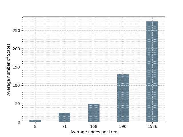
(b)

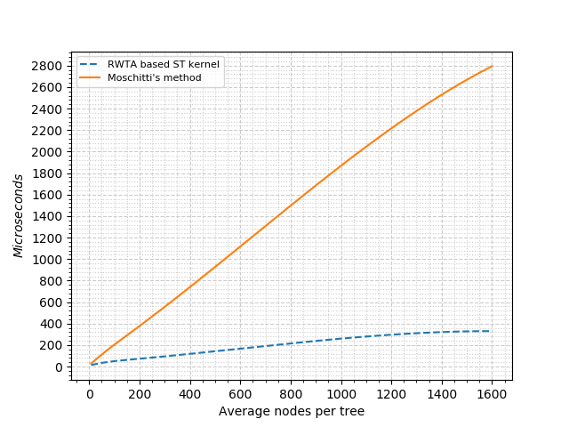
Figure 4: (a) The reduction ratio of a tree representation using RWTA approach for data set DS1. (b) The average computation time of the ST kernel when varying the tree depth for data set DS1.

(a)
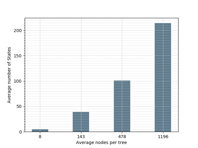
(b)

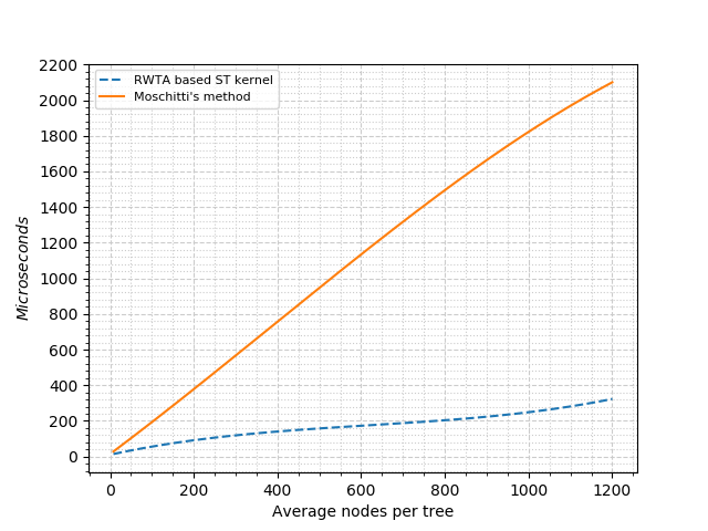
Figure 5: (a) The reduction ratio of a tree representation using RWTA approach for data set DS2. (b) The average computation time of the ST kernel when varying the alphabet arity for data set DS2.

(a)
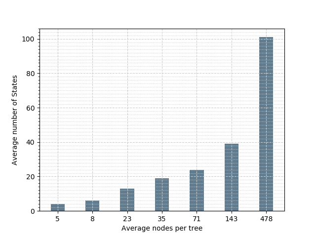
(b)

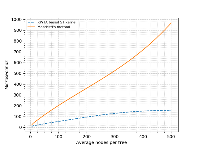
Figure 6: (a) The reduction ratio of a tree representation using RWTA approach for data set DS3. (b) The average computation time of the ST kernel when varying the tree depth and the alphabet arity for data set DS3.

References

-
[1]
M. A. Aizerman, E. M. Braverman, L. I. Rozonoèr,
Theoretical foundation of potential
functions method in pattern recognition, Avtomat. i Telemekh. 25 (6) (1964)
917–936.
URL http://mi.mathnet.ru/at11677 -
[2]
C. Cortes, V. Vapnik,
Support-vector networks, Machine
Learning 20 (3) (1995) 273–297.
doi:10.1007/BF00994018.
URL http://dx.doi.org/10.1007/BF00994018 -
[3]
D. Zelenko, C. Aone, A. Richardella,
Kernel methods for
relation extraction, Journal of Machine Learning Research 3 (2003)
1083–1106.
URL http://www.jmlr.org/papers/v3/zelenko03a.html -
[4]
B. Schölkopf, A. J. Smola, K. Müller,
Kernel principal component
analysis, in: Artificial Neural Networks - ICANN ’97, 7th International
Conference, Lausanne, Switzerland, October 8-10, 1997, Proceedings, 1997, pp.
583–588.
doi:10.1007/BFb0020217.
URL http://dx.doi.org/10.1007/BFb0020217 -
[5]
M. Collins, N. Duffy, New
ranking algorithms for parsing and tagging: Kernels over discrete structures,
and the voted perceptron, in: Proceedings of the 40th Annual Meeting of the
Association for Computational Linguistics, July 6-12, 2002, Philadelphia, PA,
USA., 2002, pp. 263–270.
URL http://www.aclweb.org/anthology/P02-1034.pdf -
[6]
A. Culotta, J. S. Sorensen,
Dependency
tree kernels for relation extraction, in: Proceedings of the 42nd Annual
Meeting of the Association for Computational Linguistics, 21-26 July, 2004,
Barcelona, Spain., 2004, pp. 423–429.
URL http://acl.ldc.upenn.edu/acl2004/main/pdf/244_pdf_2-col.pdf -
[7]
C. M. Cumby, D. Roth,
On kernel methods
for relational learning, in: Machine Learning, Proceedings of the Twentieth
International Conference (ICML 2003), August 21-24, 2003, Washington, DC,
USA, 2003, pp. 107–114.
URL http://www.aaai.org/Library/ICML/2003/icml03-017.php -
[8]
A. Moschitti,
A study on
convolution kernels for shallow statistic parsing, in: Proceedings of the
42nd Annual Meeting of the Association for Computational Linguistics, 21-26
July, 2004, Barcelona, Spain., 2004, pp. 335–342.
URL http://acl.ldc.upenn.edu/acl2004/main/pdf/388_pdf_2-col.pdf -
[9]
S. Filice, G. Da San Martino, A. Moschitti,
Structural representations
for learning relations between pairs of texts, in: Proceedings of the 53rd
Annual Meeting of the Association for Computational Linguistics and the 7th
International Joint Conference on Natural Language Processing (Volume 1: Long
Papers), Association for Computational Linguistics, Beijing, China, 2015, pp.
1003–1013.
doi:10.3115/v1/P15-1097.
URL https://www.aclweb.org/anthology/P15-1097 -
[10]
H. Wachsmuth, N. Naderi, Y. Hou, Y. Bilu, V. Prabhakaran, T. A. Thijm,
G. Hirst, B. Stein,
Computational argumentation
quality assessment in natural language, in: Proceedings of the 15th
Conference of the European Chapter of the Association for Computational
Linguistics: Volume 1, Long Papers, Association for Computational
Linguistics, Valencia, Spain, 2017, pp. 176–187.
URL https://www.aclweb.org/anthology/E17-1017 - [11] D. Haussler, Convolution kernels on discrete structures, Tech. rep., Technical report, Department of Computer Science, University of California … (1999).
- [12] S. Vishwanathan, A. J. Smola., Fast kernels on strings and trees, Advances on Neural Information Proccessing Systems, (2002) 14.
- [13] A. Moschitti, Efficient convolution kernels for dependency and constituent syntactic trees, in: ECML, Vol. 4212 of Lecture Notes in Computer Science, Springer, 2006, pp. 318–329.
- [14] H. Kashima, T. Koyanagi, Kernels for semi-structured data, in: ICML, Morgan Kaufmann, 2002, pp. 291–298.
- [15] D. Kimura, T. Kuboyama, T. Shibuya, H. Kashima, A subpath kernel for rooted unordered trees, in: PAKDD (1), Vol. 6634 of Lecture Notes in Computer Science, Springer, 2011, pp. 62–74.
- [16] D. S. M. G., Kernel methods for tree structured data, PhD thesis (2009).
-
[17]
A. Moschitti, Making tree
kernels practical for natural language learning, in: EACL 2006, 11st
Conference of the European Chapter of the Association for Computational
Linguistics, Proceedings of the Conference, April 3-7, 2006, Trento, Italy,
2006, pp. 113–120.
URL http://acl.ldc.upenn.edu/E/E06/E06-1015.pdf -
[18]
R. Azaïs, F. Ingels, The weight
function in the subtree kernel is decisive, Journal of Machine Learning
Research 21 (2020) 1–36.
URL https://jmlr.org/papers/v21/19-290.html - [19] F. Aiolli, G. Da San Martino, A. Sperduti, A. Moschitti, Efficient kernel-based learning for trees, in: 2007 IEEE Symposium on Computational Intelligence and Data Mining, 2007, pp. 308–315. doi:10.1109/CIDM.2007.368889.
-
[20]
M. Droste, P. Gastin,
Weighted automata and
weighted logics, Theor. Comput. Sci. 380 (1-2) (2007) 69–86.
doi:10.1016/j.tcs.2007.02.055.
URL http://dx.doi.org/10.1016/j.tcs.2007.02.055 -
[21]
M. Droste, H. Vogler,
Weighted tree automata and
weighted logics, Theor. Comput. Sci. 366 (3) (2006) 228–247.
doi:10.1016/j.tcs.2006.08.025.
URL http://dx.doi.org/10.1016/j.tcs.2006.08.025 - [22] F. Aiolli, G. D. S. Martino, A. Sperduti, An efficient topological distance-based tree kernel, IEEE Transactions on Neural Networks and Learning Systems 26 (2015) 1115–1120.
- [23] F. Ouardi, Subtree kernel computation using rwta, https://github.com/ouardifaissal/Subtree-kernel-computation-using-RWTA (2021).
- [24] Y. Han, D. Wood, Generalizations of 1-deterministic regular languages, Information and Computation 206 (9-10) (2008) 1117–1125. doi:10.1016/j.ic.2008.03.013.