Interventional and Counterfactual Inference
with Diffusion Models

Abstract

We consider the problem of answering observational, interventional, and counterfactual queries in a causally sufficient setting where only observational data and the causal graph are available. Utilizing the recent developments in diffusion models, we introduce diffusion-based causal models (DCM) to learn causal mechanisms, that generate unique latent encodings. These encodings enable us to directly sample under interventions and perform abduction for counterfactuals. Diffusion models are a natural fit here, since they can encode each node to a latent representation that acts as a proxy for exogenous noise. Our empirical evaluations demonstrate significant improvements over existing state-of-the-art methods for answering causal queries. Furthermore, we provide theoretical results that offer a methodology for analyzing counterfactual estimation in general encoder-decoder models, which could be useful in settings beyond our proposed approach.

1 Introduction

Understanding the causal relationships in complex problems is crucial for making analyses, conclusions, and generalized predictions. To achieve this, we require causal models and queries. Structural Causal Models (SCMs) are generative models describing the causal relationships between variables, allowing for observational, interventional, and counterfactual queries (Pearl, 2009a). An SCM specifies how a set of endogenous (observed) random variables is generated from a set of exogenous (unobserved) random variables with prior distribution via a set of structural equations.

In this work, we focus on approximating SCM given observational data and the underlying causal DAG. Our aim is to provide a mechanism for answering all the three types of causal (observational, interventional, and counterfactual) queries. For this, we assume causal sufficiency, i.e., absence of hidden confounders.

In the SCM framework, causal queries can be answered by learning a proxy for the unobserved exogenous noise and the structural equations. This suggests that learning (conditional) latent variable models could be an attractive choice for the modeling procedure, as the latent serves as the proxy for the exogenous noise. In these models, the encoding process extracts the latent from an observation, and the decoding process generates the sample from the latent, approximating the structural equations.

Our Contributions. In this work, we propose and analyze the effectiveness of using a diffusion model for modeling SCMs. Diffusion models (Sohl-Dickstein et al., 2015; Ho et al., 2020; Song et al., 2021) have gained popularity recently due to their high expressivity and exceptional performance in generative tasks (Saharia et al., 2022; Ramesh et al., 2022; Kong et al., 2021). Our key idea is to model each node in the causal graph as a diffusion model and cascade generated samples in topological order to answer causal queries. For each node, the corresponding diffusion model takes as input the node and parent values to encode and decode a latent representation. To implement the diffusion model, we utilize the recently proposed Denoising Diffusion Implicit Models (DDIMs) (Song et al., 2021), which may be interpreted as a deterministic autoencoder model with latent variables. We refer to the resulting model as diffusion-based causal model (DCM) and show that this model mimics the necessary properties of an SCM. Our key contributions include:

• [Section 3] We propose diffusion-based causal model (DCM), a new model class for modeling structural causal models, that provides a flexible and practical framework for approximating both interventions (do-operator) and counterfactuals (abduction-action-prediction steps). We present a procedure for training a DCM given just the causal graph and observational data, and show that the resulting trained model enables sampling from the observational and interventional distributions, and facilitates answering counterfactual queries.

• [Section 4] Our theoretical analysis examines the accuracy of counterfactual estimates generated by the DCM, and we demonstrate that they can be bounded given some reasonable assumptions. Importantly, our analysis is not limited to diffusion models, but also applies to other encoder-decoder settings. These error bounds represent an initial effort to explain the observed performance improvements in using latent variable models, like diffusion models, to address counterfactual queries.

• [Section 5] We evaluate the performance of DCM on a range of synthetic datasets generated with various structural equation types for all three forms of causal queries. We find that DCM consistently outperforms existing state-of-the-art methods (Sánchez-Martín et al., 2021; Khemakhem et al., 2021). In fact, for certain interventional and counterfactual queries such as those arising with nonadditive noise models, DCM is better by an order of magnitude or more than these existing approaches. Additionally, we demonstrate the favorable performance of DCM on an interventional query experiment conducted on fMRI data.

Related Work. Over the years, a variety of methods have been developed in the causal inference literature for answering interventional and/or counterfactual queries including non-parametric methods (Shalit et al., 2017; Alaa and Van Der Schaar, 2017; Muandet et al., 2021) and probabilistic modeling methods (Zečević et al., 2021a). More relevant to our approach is a recent series of work, including (Moraffah et al., 2020; Pawlowski et al., 2020; Kocaoglu et al., 2018; Parafita and Vitrià, 2020; Zečević et al., 2021b; Garrido et al., 2021; Karimi et al., 2020; Sánchez-Martín et al., 2021; Khemakhem et al., 2021; Sanchez and Tsaftaris, 2022) that have demonstrated the success of using deep (conditional) generative models for this task.

Karimi et al. (2020) propose an approach for answering interventional queries by fitting a conditional variational autoencoder to each conditional in the Markov factorization implied by the causal graph. Also using the ideas of variational inference and normalizing flows, Pawlowski et al. (2020) propose schemes for counterfactual inference.

In Khemakhem et al. (2021), the authors propose an autoregressive normalizing flow for causal discovery and queries, referred to as CAREFL. While the authors focus on bivariate graphs between observed and unobserved variables, their approach can be extended to more general DAGs. However, as also noted by Sánchez-Martín et al. (2021), CAREFL is unable to exploit the absence of edges fully as it reduces a causal graph to its causal ordering (which may not be unique). Sánchez-Martín et al. (2021) propose VACA, which uses graph neural networks (GNNs) in the form of a variational graph autoencoder to sample from the observational, interventional, and counterfactual distribution. VACA can utilize the inherent graph structure through the GNN, however, suffers in empirical performance (see Section 5). Furthermore, the usage of the GNN leads to undesirable design constraints, e.g., the encoder GNN cannot have hidden layers (Sánchez-Martín et al., 2021).

Sanchez and Tsaftaris (2022) also use diffusion models for counterfactual estimation, focusing on the bivariate graph case with an image class causing an image. The authors train a diffusion model to generate images and use the abduction-action-prediction procedure from Pearl et al. (2016) as well as classifier guidance (Dhariwal and Nichol, 2021) to generate counterfactual images. However, this is solely for bivariate models and requires training a separate classifier for intermediate diffusion images, and exhibits poor performance for more complex images e.g., ImageNet (Deng et al., 2009). We generalize their approach to arbitrary causal graphs, utilize classifier-free guidance (Ho and Salimans, 2021), and additionally handle observational and interventional queries.

2 Preliminaries

Notation. To distinguish random variables from their instantiation, we represent the former with capital letters and the latter with the corresponding lowercase letters. To distinguish between the nodes in the causal graph and diffusion random variables, we use subscripts to denote graph nodes. Let $[n]:=\{1,\ldots,n\}$.

Structural Causal Models. Consider a directed acyclic graph (DAG) $\mathcal{G}$ with nodes $\{1,\dots,K\}$ in a topologically sorted order, where a node $i$ is represented by a (random) variable $X_{i}$ in some generic space $\mathcal{X}_{i}\subset\mathbb{R}^{d_{i}}$. Let $\mathrm{pa}_{i}$ be the parents of node $i$ in $\mathcal{G}$ and let $X_{\mathrm{pa}_{i}}\coloneqq\{X_{j}\}_{j\in\mathrm{pa}_{i}}$ be the variables of the parents of node $i$. A structural causal model $\mathcal{M}$ describes the relationship between an observed/endogenous node $i$ and its causal parents. Formally, an SCM $\mathcal{M}:=(\mathbf{F},p(\mathbf{U}))$ determines how a set of $K$ endogenous random variables $\mathbf{X}:=\{X_{1},\dots,X_{K}\}$ is generated from a set of exogenous random variables $\mathbf{U}:=\{U_{1},\dots,U_{K}\}$ with prior distribution $p(\mathbf{U})$ via a set of structural equations, $\mathbf{F}:=(f_{1},\ldots,f_{K})$ where $X_{i}:=f_{i}(X_{\mathrm{pa}_{i}},U_{i})$ for $i\in[K]$. Throughout this paper, we assume that the unobserved random variables are jointly independent (Markovian SCM), and the DAG $\mathcal{G}$ is the graph induced by $\mathcal{M}$. Every SCM $\mathcal{M}$ entails a unique joint observational distribution satisfying the causal Markov assumption: $p(\mathbf{X})=\prod_{i=1}^{K}p(X_{i}\mid X_{\mathrm{pa}_{i}})$.

Structural causal models address Pearl’s causal hierarchy (or “ladder of causation”), which consists of three “layers” of causal queries in increasing complexity (Pearl, 2009a): observational (or associational), interventional, and counterfactual. As an example, an interventional query can be formulated as “What will be the effect on the population $\mathbf{X}$, if a variable $X_{i}$ is assigned a fixed value $\gamma_{i}$?” The do-operator $\mathrm{do}(X_{i}:=\gamma_{i})$ represents the effect of setting variable $X_{i}$ to $\gamma_{i}$. Note that our proposed framework allows for more general sets of interventions as well, such as interventions on multiple variables denoted as $\mathrm{do}(X_{\mathcal{I}}:=\gamma)$ (where $\mathcal{I}\subseteq[K]$, $X_{\mathcal{I}}:=(X_{i})_{i\in\mathcal{I}}$, $\gamma\in\mathbb{R}^{|\mathcal{I}|}$). An intervention operation, $\mathrm{do}(X_{\mathcal{I}}:=\gamma)$, transforms the original joint distribution into an interventional distribution denoted by $p(\mathbf{X}\mid\mathrm{do}(X_{\mathcal{I}}:=\gamma))$. On the other hand, a counterfactual query can be framed as “What would have been the outcome of a particular factual sample $x^{\mathrm{F}}:=(x_{1}^{\mathrm{F}},\dots,x_{K}^{\mathrm{F}})$, if the value of $X_{\mathcal{I}}$ had been set to $\gamma$?”. Counterfactual estimation may be performed through the three-step procedure of 1) abduction: estimation of the exogenous noise $U$, 2) action: intervene $\mathrm{do}(X_{\mathcal{I}}:=\gamma)$, and 3) prediction: estimating $x^{\text{CF}}$ using the abducted noise and intervention values.

Diffusion Models. Given data from distribution $X^{0}\sim Q$, the objective of diffusion models is to construct an efficiently sampleable distribution approximating $Q$. Denoising diffusion probabilistic models (DDPMs) (Sohl-Dickstein et al., 2015; Ho et al., 2020) accomplish this by introducing a forward noising process that adds isotropic Gaussian noise at each time step and a learned reverse denoising process. A common representation of diffusion models is a fixed Markov chain that adds Gaussian noise with variances $\beta_{1},\ldots,\beta_{T}\in(0,1)$, generating latent variables $X^{1},\ldots,X^{T}$,

$$q(X^{t}\mid x^{t-1}) =\mathcal{N}(X^{t};\sqrt{1-\beta_{t}}x^{t-1},\beta_{t}I)$$

$$q(X^{t}\mid x^{0}) =\mathcal{N}(X^{t};\sqrt{\alpha_{t}}x^{0},(1-\alpha_{t})I)$$

where $\alpha_{t}:=\prod_{i=1}^{t}(1-\beta_{i})$. Here, $T\in\mathbb{Z}^{+}$, and $t\in\{0,\dots,T\}$ denotes the time index.

By choosing sufficiently large $T$ and $\alpha_{t}$ that converge to $0$, we have $X^{T}$ is distributed as an isotropic Gaussian distribution. The learned reverse diffusion process attempts to approximate the intractable $q(X^{t-1}\mid x^{t})$ using a neural network and is defined as a Markov chain with Gaussian transitions,

$$p_{\theta}(X^{t-1}\mid x^{t})=\mathcal{N}(X^{t-1};\mu_{\theta}(x^{t},t),\Sigma_{\theta}(x^{t},t)).$$

Rather than predicting $\mu_{\theta}$ directly, the network could instead predict the Gaussian noise $\varepsilon$ from $x^{t}=\sqrt{\alpha_{t}}x^{0}+\sqrt{1-\alpha_{t}}\varepsilon$. Ho et al. (2020) found that modeling $\varepsilon$ instead of $\mu_{\theta}$, fixing $\Sigma_{\theta}$, and using the following reweighted loss function

$$\mathbb{E}_{\mathrel{\begin{subarray}{c}t\sim\mathrm{Unif}\{[T]\}\\ X^{0}\sim Q\\ \varepsilon\sim\mathcal{N}(0,I)\end{subarray}}}[\|\varepsilon-\varepsilon_{\theta}(\sqrt{\alpha_{t}}X^{0}+\sqrt{1-\alpha_{t}}\varepsilon,t)\|^{2}],$$ (1)

works well empirically. We also utilize this loss function in our training.

Song et al. (2021) introduce a richer family of distributions, where it is possible to use a pretrained DDPM model to obtain a deterministic sample given noise $X^{T}$, known as the denoising diffusion implicit model (DDIM), with reverse implicit diffusion process

$$\begin{split}X^{t-1}&:=\sqrt{\frac{\alpha_{t-1}}{\alpha_{t}}}X^{t}-\varepsilon_{\theta}(X^{t},t)\left(\sqrt{\alpha_{t-1}(1-\alpha_{t})/\alpha_{t}}-\sqrt{1-\alpha_{t-1}}\right).\end{split}$$ (2)

Note that the $X^{t}$ here is deterministic. We also use a forward implicit diffusion process introduced by Song et al. (2021), derived from rewriting the DDIM process Eq. (2) as an ordinary differential equation (ODE) and considering the Euler method approximation in the forward direction to obtain

$$\begin{split}X^{t+1}&:=\sqrt{\frac{\alpha_{t+1}}{\alpha_{t}}}X^{t}+\varepsilon_{\theta}(X^{t},t)\left(\sqrt{1-\alpha_{t+1}}-\sqrt{\alpha_{t+1}(1-\alpha_{t})/\alpha_{t}}\right).\end{split}$$ (3)

We utilize the DDIM framework in this work, in particular Eqs. (3) and (2) will define the encoding (forward) and decoding (reverse) processes.

3 DCMs: Diffusion-based Causal Models

In this section, we present our DCM approach for modeling the SCMs and to answer causal queries. We first explain the construction and the training process of a DCM, and then explain how the model can be used for answering various causal queries. We start with some notations.

• Define $Z_{i}^{t}$ to be the $i$th endogenous node value at diffusion step $t$ of the forward implicit diffusion process (Eq. (3)), and let $Z_{i}\coloneqq Z_{i}^{T}$.

• Define $\hat{X}_{i}^{t}$ to be $i$th endogenous node value at diffusion step $t$ of the reverse implicit diffusion process (Eq. (2)), and let $\hat{X}_{i}\coloneqq\hat{X}_{i}^{0}$.

Training a DCM. We train a diffusion model for each node, taking denoised parent values as input. The parent values can be interpreted as additional covariates to the model, where one may choose to use classifier free guidance to incorporate the covariates (Ho and Salimans, 2021). Empirically, we find that simply concatenating the covariates results in better performance than classifier free guidance.

We use the $\varepsilon_{\theta}$ parametrization for the diffusion model from Ho et al. (2020), representing the diffusion model for node $i$ as $\varepsilon_{\theta}^{i}(X,X_{\mathrm{pa}_{i}},t)$. The complete training procedure presented in Algorithm 1 is only slightly modified from the usual training procedure, with the additions of the parents as covariates and training a diffusion model for each node. Since the generative models learned for generation of different endogenous nodes do not affect training of each other, these models may be trained in parallel. Our final DCM model is just a combination of these $K$ trained diffusion models $\varepsilon_{\theta}^{1},\dots,\varepsilon_{\theta}^{K}$.

Algorithm 1 DCM Training

Input: Distribution $Q$, scale factors $\{\alpha_{t}\}_{t=1}^{T}$, causal DAG $\mathcal{G}$ with node $i$ represented by $X_{i}$

1:while not converged do

2:   Sample $X^{0}\sim Q$

3:   for $i=1,\ldots,K$ do

4:      $t\sim\mathrm{Unif}[\{1,\ldots,T\}]$

5:      $\varepsilon\sim\mathcal{N}(0,I_{d_{i}})$ {$d_{i}$ is the dimension of $X_{i}$}

6:      Update parameters of node $i$’s diffusion model $\varepsilon_{\theta}^{i}$, by minimizing the following loss:                                        $\|\varepsilon-\varepsilon_{\theta}^{i}(\sqrt{\alpha_{t}}X_{i}^{0}+\sqrt{1-\alpha_{t}}\varepsilon,X_{\mathrm{pa}_{i}}^{0},t)\|_{2}^{2}$ (based on Eq. (1))

7:   end for

8:end while

We use all the variables $(X_{1},\ldots,X_{K})$ for the training procedure, because a priori, we do not assume anything on the possible causal queries, i.e., we allow for all possible target variables, intervened variables, etc. However, if we are only interested in some pre-defined set of queries, then the graph could be reduced accordingly. For example, if we are only interested in counterfactual estimate of a particular node with respect to an intervention of a predecessor, one can simply reduce it to a subgraph containing the target node, the intervened node and a backdoor adjustment set (e.g., the ancestors of the intervened node). This then reduces to only learning a single diffusion model.

Encoding and Decoding Steps with DCM. With a DCM, the encoding (resp. decoding) process is identical to the DDIM encoding (resp. decoding) process except we include the parent values as additional covariates. Let us focus on a node $i\in[K]$ (same process is repeated for each node $i$). The encoding process takes $X_{i}$ and its parent values $X_{\mathrm{pa}_{i}}$ as input and maps it to a latent variable $Z_{i}$. The decoding process takes $Z_{i}$ and $X_{\mathrm{pa}_{i}}$ as input to construct $\hat{X}_{i}$ (an approximation of $X_{i}$). Formally, using the forward implicit diffusion process in Eq. (3), given a sample $X_{i}$, we encode a unique latent variable $Z_{i}:=Z_{i}^{T}$, using the recursive formula

$$Z^{t+1}_{i}:=\sqrt{\frac{\alpha_{t+1}}{\alpha_{t}}}Z^{t}_{i}+\varepsilon_{\theta}^{i}(Z^{t}_{i},X_{\mathrm{pa}_{i}},t)\left(\sqrt{1-\alpha_{t+1}}-\sqrt{\frac{\alpha_{t+1}(1-\alpha_{t})}{\alpha_{t}}}\right),\forall t=0,..,T-1,$$ (4)

where $Z_{i}^{0}:=X_{i}$. The latent variable $Z_{i}$ acts as a proxy for the exogenous noise $U_{i}$. Using the reverse implicit diffusion process from DDIM in Eq. (2), given a latent vector $Z_{i}$ we obtain a deterministic decoding $\hat{X}_{i}:=\hat{X}_{i}^{0}$, using the recursive formula

$$\hat{X}^{t-1}_{i}:=\sqrt{\frac{\alpha_{t-1}}{\alpha_{t}}}\hat{X}^{t}_{i}-\varepsilon_{\theta}^{i}(\hat{X}_{i}^{t},X_{\mathrm{pa}_{i}},t)\left(\sqrt{\frac{\alpha_{t-1}(1-\alpha_{t})}{\alpha_{t}}}-\sqrt{1-\alpha_{t-1}}\right),\forall t=T,..,1,$$ (5)

where $\hat{X}^{T}:=Z_{i}$. In the following, we use $\mathsf{Enc}_{i}(X_{i},X_{\mathrm{pa}_{i}})$ and $\mathsf{Dec}_{i}(Z_{i},X_{\mathrm{pa}_{i}})$ to denote the encoding and decoding functions for node $i$ defined in Eqns. (4) and (5) respectively. See Algorithms 4 and 5 for detailed pseudocodes.

Answering Causal Queries with a Trained DCM. We now describe how a trained DCM model can be used for (approximately) answering causal queries. Answering observational and interventional queries require sampling from the observational and the interventional distribution respectively. With counterfactuals, a query is at the unit level, where the structural assignments are changed, but the exogenous noise is identical to that of the observed datum.

(a) Generating Samples for Observational/Interventional Queries. Samples from a DCM model that approximates the interventional distribution $p(\mathbf{X}\mid\mathrm{do}(X_{\mathcal{I}}:=\gamma))$ can be generated as follows. For an intervened node $i$ with intervention $\gamma_{i}$, the sampled value is always the intervention value, therefore we generate $\hat{X}_{i}:=\gamma_{i}$. For a non-intervened node $i$, assume by induction we have the generated parent values $\hat{X}_{\mathrm{pa}_{i}}$. To generate $\hat{X}_{i}$, we first sample the latent vector $Z_{i}\sim\mathcal{N}(0,I_{d_{i}})$ where $d_{i}$ is the dimension of $X_{i}$. Then taking $Z_{i}$ as the noise for node $i$, we compute $\hat{X}_{i}:=\mathsf{Dec}_{i}(Z_{i},\hat{X}_{\mathrm{pa}_{i}})$ as the generated sample value for node $i$. This value $\hat{X}_{i}$ is then used as the parent value for the children of node $i$. Samples from a DCM model that approximates the observational distribution $p(\mathbf{X})$ can be generated by setting $\mathcal{I}=\emptyset$ (see Algorithm 2).

Algorithm 2 Observational/Interventional Sampling

Input: Intervention set $\mathcal{I}$ with values $\gamma$ ($I=\emptyset$ for observational sampling)

1:for $i=1,\ldots,K$ do {in topological order}

2:   $Z_{i}\sim\mathcal{N}(0,I_{d_{i}})$

3:   if $i\in\mathcal{I}$ then

4:      $\hat{X}_{i}\leftarrow\gamma_{i}$

5:   else

6:      $\hat{X}_{i}\leftarrow\mathsf{Dec}_{i}(Z_{i},\hat{X}_{\mathrm{pa}_{i}})$

7:   end if

8:end for

9:Return $\hat{X}:=(\hat{X}_{1},\dots,\hat{X}_{K})$

Algorithm 3 Counterfactual Inference

Input: Intervention set $\mathcal{I}$ with values $\gamma$, factual sample $x^{\mathrm{F}}:=(x_{1}^{\mathrm{F}},\dots,x_{K}^{\mathrm{F}})$

1:for $i=1,\ldots,K$ do {in topological order}

2:   if $i\in\mathcal{I}$ then

3:      $\hat{x}^{\mathrm{CF}}_{i}\leftarrow\gamma_{i}$

4:   else if $i$ is not a descendant of any intervened node in $\mathcal{I}$ then

5:      $\hat{x}^{\mathrm{CF}}_{i}\leftarrow x^{\mathrm{F}}_{i}$

6:   else

7:      $z^{\mathrm{F}}_{i}\leftarrow\mathsf{Enc}_{i}(x^{\mathrm{F}}_{i},x_{\mathrm{pa}_{i}}^{\mathrm{F}})$ {abduction step}

8:      $\hat{x}^{\mathrm{CF}}_{i}\leftarrow\mathsf{Dec}_{i}(z_{i},\hat{x}_{\mathrm{pa}_{i}})$ {action and prediction steps}

9:   end if

10:end for

11:Return $\hat{x}^{\mathrm{CF}}:=(\hat{x}^{\mathrm{CF}}_{1},\dots,\hat{x}^{\mathrm{CF}}_{K})$

(b) Counterfactual Queries. Consider a factual observation $x^{\mathrm{F}}:=(x_{1}^{\mathrm{F}},\dots,x_{K}^{\mathrm{F}})$ and interventions on a set of nodes $\mathcal{I}$ with values $\gamma$. We use a DCM model to construct a counterfactual estimate $\hat{x}^{\mathrm{CF}}$ as follows. The counterfactual estimate only differs from the factual value on intervened nodes or descendants of an intervened node. Similarly to interventional queries, for each intervened node $i\in\mathcal{I}$, $\hat{x}_{i}^{\mathrm{CF}}:=\gamma_{i}$. For each non-intervened node $i$ that is a descendant of any intervened node, assume by induction that we have the generated counterfactual estimates $\hat{x}_{\mathrm{pa}_{i}}^{\mathrm{CF}}$. To obtain $\hat{x}_{i}^{\mathrm{CF}}$, we first define the estimated factual noise as $\hat{z}_{i}^{\mathrm{F}}:=\mathsf{Enc}_{i}(x_{i}^{\mathrm{F}},x_{\mathrm{pa}_{i}}^{\mathrm{F}})$. Then we generate our counterfactual estimate by using $\hat{z}_{i}^{\mathrm{F}}$ as the noise for node $i$, by decoding, $\hat{x}_{i}^{\mathrm{CF}}:=\mathsf{Dec}_{i}(\hat{z}_{i}^{\mathrm{F}},\hat{x}_{\mathrm{pa}_{i}}^{\mathrm{CF}})$ (see Algorithm 3).

Note that with $x^{\mathrm{F}}$, we assumed full observability,​ since because Algorithm 3 produces a counterfactual estimate for each node. However, when intervening on $X_{\mathcal{I}}$ and if the only quantity of interest is counterfactual on some $X^{\star}$, then you only need factual samples from $\{X_{i}:X_{i}\text{ is on a path from }X_{\mathcal{I}}\to X^{\star}\}$ (Saha and Garain, 2022). In practice, this could be further relaxed by imputing for missing data, which is beyond the scope of this work.

Algorithm 4 $\mathsf{Enc}_{i}(X_{i},X_{\mathrm{pa}_{i}})$

Input: $X_{i}$, $X_{\mathrm{pa}_{i}}$

1:$Z_{i}^{0}\leftarrow X_{i}$

2:for $t=0,\ldots,T-1$ do

3:   $Z^{t+1}_{i}\leftarrow\sqrt{\frac{\alpha_{t+1}}{\alpha_{t}}}Z^{t}_{i}+\varepsilon_{\theta}^{i}(Z^{t}_{i},X_{\mathrm{pa}_{i}},t)\left(\sqrt{1-\alpha_{t+1}}-\sqrt{\frac{\alpha_{t+1}(1-\alpha_{t})}{\alpha_{t}}}\right)$

4:end for

5:Return $Z_{i}\coloneqq Z_{i}^{T}$

Algorithm 5 $\mathsf{Dec}_{i}(Z_{i},X_{\mathrm{pa}_{i}})$

Input: $Z_{i}$, $X_{\mathrm{pa}_{i}}$

1:$\hat{X}^{T}\leftarrow Z_{i}$

2:for $t=T,\ldots,1$ do

3:   $\hat{X}^{t-1}_{i}\leftarrow\sqrt{\frac{\alpha_{t-1}}{\alpha_{t}}}\hat{X}^{t}_{i}-\varepsilon_{\theta}^{i}(\hat{X}_{i}^{t},X_{\mathrm{pa}_{i}},t)\left(\sqrt{\frac{\alpha_{t-1}(1-\alpha_{t})}{\alpha_{t}}}-\sqrt{1-\alpha_{t-1}}\right)$

4:end for

5:Return $\hat{X}_{i}\coloneqq\hat{X}_{i}^{0}$

4 Bounding Counterfactual Error

We now establish sufficient conditions under which the counterfactual estimation error can be bounded. In fact, the results in this section not only hold for diffusion models, but to a more general setting of conditional latent variable models satisfying certain properties. All proofs from this section are collected in Appendix A.

We focus on learning a single conditional latent variable model for an endogenous node $X_{i}$, given its parents $X_{\mathrm{pa}_{i}}$, as the models learned for different endogenous nodes do not affect each other. Since the choice of node $i$ plays no role, we drop the subscript $i$ in the following and refer to the node of interest as $X$, its causal parents as $X_{\mathrm{pa}}$, its corresponding exogenous variables as $U$, and its structural equation as $X:=f(X_{\mathrm{pa}},U)$. Let the encoding function $g:\mathcal{X}\times\mathcal{X}_{\mathrm{pa}}\to\mathcal{Z}$ and the decoding function $h:\mathcal{Z}\times\mathcal{X}_{\mathrm{pa}}\to\mathcal{X}$, where $\mathcal{Z}$ is the latent space. In the DCM context, the functions $g$ and $h$ correspond to $\mathsf{Enc}$ and $\mathsf{Dec}$ functions, respectively.

It is well-known that that certain counterfactual queries are not identifiable from observational data without making assumptions on the functional relationships, even under causal sufficiency (Pearl, 2009b). Consequently, recent research has been directed towards understanding the conditions under which identifiability results can be obtained (Lu et al., 2020; Nasr-Esfahany and Kiciman, 2023; Nasr-Esfahany et al., 2023). Assumption 2 of our Theorem 1, ensures that the true counterfactual outcome is identifiable, see e.g., (Lu et al., 2020, Theorem 1) or (Nasr-Esfahany and Kiciman, 2023, Theorem 5). In the context of learned structural causal models to determine whether a given counterfactual query can be answered with sufficient accuracy, requires also assumptions on the learned SCM, e.g., encoder and decoder in this case.

Our first result presents sufficient conditions on the latent variable encoding function and the structural equation under which we can recover latent exogenous variable up to a (possibly nonlinear) invertible function. For simplicity, we start with a one-dimensional exogenous noise $U$ and variable $X\in\mathcal{X}\subset\mathbb{R}$. We provide a similar theorem for the multivariate case where $X\in\mathbb{R}^{m}$ for $m\geq 3$ in Theorem 2 in the Appendix A.1 with a stronger assumption on the Jacobian of $f$ and $g$.

Theorem 1.

Assume for $X\in\mathcal{X}\subset\mathbb{R}$ and exogenous noise $U\sim\mathrm{Unif}[0,1]$, $X$ satisfies the structural equation: $X:=f(X_{\mathrm{pa}},U)$, where $X_{\mathrm{pa}}\in\mathcal{X}_{\mathrm{pa}}\subset\mathbb{R}^{d}$ are the parents of node $X$ and $U\perp\!\!\!\perp X_{\mathrm{pa}}$. Consider an encoder-decoder model with encoding function $g:\mathcal{X}\times\mathcal{X}_{\mathrm{pa}}\to\mathcal{Z}$ and decoding function $h:\mathcal{Z}\times\mathcal{X}_{\mathrm{pa}}\to\mathcal{X}$, $Z:=g(X,X_{\mathrm{pa}}),\quad\hat{X}:=h(Z,X_{\mathrm{pa}})$. Assume the following conditions:

• The encoding is independent of the parent values, $g(X,X_{\mathrm{pa}})\perp\!\!\!\perp X_{\mathrm{pa}}.$

• The structural equation $f$ is differentiable and strictly increasing with respect to $U$.

• The encoding $g$ is invertible and differentiable with respect to $X$.

Then, $g(X,X_{\mathrm{pa}})=\tilde{q}(U)$ for an invertible function $\tilde{q}$.

Discussion on Assumptions Underlying Theorem 1.

(1) Assumption 1 of independence between the encoding and the parent values may appear strong, but is in fact often valid. For example, in the additive noise setting with $X:=f(X_{\mathrm{pa}})+U$ where $X_{\mathrm{pa}}$ and $U$ are independent, if the fitted model $\hat{f}\equiv f$, then the encoder $g(X,X_{\mathrm{pa}})=X-\hat{f}(X_{\mathrm{pa}})=U$ and by definition $U$ is independent of $X_{\mathrm{pa}}$. The same assumption also appears in other related results on counterfactual identifiability in bijective SCMs, see, e.g., (Nasr-Esfahany et al., 2023, Theorem 5.3) and proof of Theorem 5 in (Nasr-Esfahany and Kiciman, 2023). We conduct empirical tests to further confirm this assumption by examining the dependence between the parents and encoding values. Our experimental results show that DCMs consistently fail to reject the null hypothesis of independence. This implies that independent encodings can be found in practice. We provide the details of these experiments in Appendix B.​.

(2) Assumption 2 is always satisfied under the additive noise model (i.e., $X:=f(X_{\mathrm{pa}})+U$) and post non-linear models (Zhang and Hyvarinen, 2012). Again, the recent results about counterfactual identifiability, e.g., (Nasr-Esfahany and Kiciman, 2023, Theorem 5) and (Lu et al., 2020, Theorem 1), also utilize the same assumption.

(3) We may consider transformations of the uniform noise $U$ to obtain other settings, for example additive Gaussian noise. For a continuous random variable $U^{\prime}$ with invertible CDF $F$ and the structural equation $f(\cdot,F(\cdot))$, we have $U^{\prime}\stackrel{{\scriptstyle d}}{{=}}F^{-1}(U)$ and the results similarly hold.

We now discuss some consequences of Theorem 1 for estimating counterfactual outcomes.

1. Perfect Estimation. Using Theorem 1, we now look at a condition under which the counterfactual estimate produced by the encoder-decoder model matches the true counterfactual outcome.. The idea here been, if no information is lost in the encoding and decoding steps, i.e., $h(g(X,X_{\mathrm{pa}}),X_{\mathrm{pa}})=X$, and assuming Theorem 1 ($g(X,X_{\mathrm{pa}})=\tilde{q}(U)$), we have $h(\tilde{q}(U),X_{\mathrm{pa}})=X=f(X_{\mathrm{pa}},\tilde{q}^{-1}(U))$. This means that in the abduction step, the encoder-decoder model could recover $\tilde{q}(U)$, but in the prediction step with, it first applies the inverse of $\tilde{q}$ to the recovered exogenous variable, and then $f$. Thus, the counterfactual estimate equals the true counterfactual outcome.

Corollary 1.

Assume the conditions of Theorem 1. Furthermore, assume the encoder-decoder model pair $(g,h)$ satisfies: $h(g(X,X_{\mathrm{pa}}),X_{\mathrm{pa}})=X$. Consider a factual sample pair $x^{\mathrm{F}}:=(x,x_{\mathrm{pa}})$ where $x:=f(x_{\mathrm{pa}},u)$ and an intervention $\mathrm{do}(X_{\mathrm{pa}}:=\gamma)$. Then, the counterfactual estimate, given by $h(g(x,x_{\mathrm{pa}}),\gamma)$ matches the true counterfactual outcome $x^{\mathrm{CF}}:=f(\gamma,u)$.

Comparison with Recent Related Work. Recent studies by Nasr-Esfahany and Kiciman (2023) and Nasr-Esfahany et al. (2023) have explored the problem of estimating counterfactual outcomes with learned SCMs. In particular, Nasr-Esfahany and Kiciman (2023) consider a setting where the SCM $X:=f(X_{\mathrm{pa}},U)$ is learned with a bijective (deep conditional generative) model $\hat{f}(X_{\mathrm{pa}},\hat{U})$ (Nasr-Esfahany and Kiciman, 2023, Theorem 5)). Nasr-Esfahany et al. (2023, Theorem 5.3) considered a closely related problem of learning a ground-truth bijective SCM. The conditions underlying ours and these results are not directly comparable because, unlike our setup, they do not explicitly consider an encoder-decoder model. Our results provide precise conditions on the encoder $g$ and decoder $h$ for recovering the correct counterfactual outcome, and we can extend these results to obtain counterfactual estimation error bounds under relaxed assumptions, a problem that has not been addressed previously.

2. Estimation Error. Another consequence of Theorem 1 is that it can bound the counterfactual error in terms of the reconstruction error of the encoder-decoder model. Informally, the following corollary shows that if the reconstruction $h(g(X,X_{\mathrm{pa}}),X_{\mathrm{pa}})$ is “close” to $X$ (measured under some metric $d(\cdot,\cdot)$), then such encoder-decoder models can provide “good” counterfactual estimates. To the best of our knowledge, this is the first result that establishes a bound on the counterfactual error in relation to the reconstruction error of these encoder-decoder models.

Corollary 2.

Let $\gamma\geq 0$. Assume the conditions of Theorem 1. Furthermore, assume the encoder-decoder model pair $(g,h)$ under some metric $d$ (e.g., $\|\cdot\|_{2}$), has reconstruction error less than $\tau$: $d(h(g(X,X_{\mathrm{pa}}),X_{\mathrm{pa}}),X)\leq\tau$. Consider a factual sample pair $x^{\mathrm{F}}:=(x,x_{\mathrm{pa}})$ where $x:=f(x_{\mathrm{pa}},u)$ and an intervention $\mathrm{do}(X_{\mathrm{pa}}:=\gamma)$. Then, the error between the true counterfactual $x^{\mathrm{CF}}:=f(\gamma,u)$ and counterfactual estimate given by $h(g(x,x_{\mathrm{pa}}),\gamma)$ is at most $\tau$, i.e., $d(h(g(x,x_{\mathrm{pa}}),\gamma),x^{\mathrm{CF}})\leq\tau$.

The above result suggests that the reconstruction error can serve as an estimate for the counterfactual error. While the true value of $\tau$ is unknown, we may compute a reasonable bound by computing the reconstruction error over the dataset.

5 Experimental Evaluation

In this section, we evaluate the empirical performance of DCM for answering causal queries on both synthetic and real world data. Additional synthetic and semi-synthetic experimental evaluations are presented in Appendix D. For the semi-synthetic experiments, we leverage the Sachs dataset (Sachs et al., 2005).

Diffusion Model Implementation and Training. For our implementation of the $\varepsilon_{\theta}$ model in DCM, we use a simple fully connected neural network with three hidden layers of size $[128,256,256]$ and SiLU activation (Elfwing et al., 2018). We fit the model using Adam with a learning rate of 1e-4, batch size of 64, and train for 500 epochs. For root nodes, we do not train diffusion models and instead sample from the empirical distribution of the training data. Additional details about the diffusion model parameters are in Section C.1.

Compared Approaches. We primarily compare DCM to two recently proposed state-of-the-art schemes VACA (Sánchez-Martín et al., 2021) and CAREFL (Khemakhem et al., 2021), and a general regression model that assumes an additive noise model which we refer to as ANM. For VACA and CAREFL, we use the code provided by their respective authors. The ANM approach performs model selection over a variety of models, including linear and gradient boosted regressor, and we use the implementation from the popular DoWhy causal inference package (Sharma et al., 2019; Blöbaum et al., 2022). Additional details on how ANM answers causal queries are provided in Appendix C.2 and implementation details for VACA, CAREFL, and ANM are in Section C.1.

Synthetic Data Experiments. For generating quantitative results, we use synthetic experiments since we know the exact structural equations, and hence we have access to the ground-truth observational, interventional, and counterfactual distributions. We provide two sets of synthetic experiments, a set of two larger graphs provided here and a set of four smaller graphs provided in Section D.1. The two larger graphs, include a ladder graph structure (see Figure 3) and a randomly generated graph structure. Both graphs are comprised of $10$ nodes of three dimensions each, and the random graph is a randomly sampled directed acyclic graph (see Appendix C.3 for more details).

Following Sánchez-Martín et al. (2021), for the observational and interventional distributions, we report the Maximum Mean Discrepancy (MMD) (Gretton et al., 2012) between the true and estimated distributions. For counterfactual estimation, we report the mean squared error (MSE) of the true and estimated counterfactual values. Again following Sánchez-Martín et al. (2021), we consider two broad classes of structural equations:

• Additive Noise Model (NLIN): $f_{i}(X_{\mathrm{pa}_{i}},U_{i})=f^{\prime}(X_{\mathrm{pa}_{i}})+U_{i}$. In particular, we will be interested in the case where $f_{i}$’s are non-linear.

• Nonadditive Noise Model (NADD): $f_{i}(X_{\mathrm{pa}_{i}},U_{i})$ is an arbitrary function of $X_{\mathrm{pa}_{i}}$ and $U_{i}$.

To prevent overfitting of hyperparameters, we randomly generate these structural equations for each initialization. Each structural equation is comprised a neural network with a single hidden layer of 16 units and SiLU activation (Elfwing et al., 2018) with random weights from sampled from $[-1,1]$.

Each simulation generates $n=5000$ samples as training data. Let $\hat{M}$ be a fitted causal model and $M^{\star}$ be the true causal model, both capable of generating observational and interventional samples, and answering counterfactual queries. Each pair of graphs and structural equation type is evaluated for $20$ different initialization, and we report the mean value. We provide additional details about our observational, interventional, and counterfactual evaluation frameworks in Appendix C.4.

Table 1: Mean$\pm$standard deviation of observational, interventional, and counterfactual queries of the ladder and random SCMs in nonlinear and nonadditive settings over $20$ random initializations of the model and training data. The values are multiplied by $100$ for clarity.

			DCM	ANM	VACA	CAREFL
SCM		Metric	($\times 10^{-2}$)	($\times 10^{-2}$)	($\times 10^{-2}$)	($\times 10^{-2}$)
Ladder	NLIN	Obs. MMD	0.44$\pm$0.14	0.63$\pm$0.21	2.82$\pm$0.83	13.41$\pm$1.14
		Int. MMD	1.63$\pm$0.20	1.80$\pm$0.17	4.48$\pm$0.78	15.01$\pm$1.23
		CF. MSE	3.42$\pm$1.67	10.65$\pm$2.48	41.03$\pm$19.00	17.46$\pm$6.04
	NADD	Obs. MMD	0.32$\pm$0.11	0.40$\pm$0.16	3.22$\pm$1.05	14.60$\pm$1.34
		Int. MMD	1.54$\pm$0.17	1.57$\pm$0.15	5.13$\pm$1.16	16.87$\pm$1.85
		CF. MSE	4.28$\pm$2.39	10.71$\pm$5.47	27.42$\pm$12.34	22.26$\pm$13.75
Random	NLIN	Obs. MMD	0.28$\pm$0.12	0.47$\pm$0.15	1.82$\pm$0.73	12.11$\pm$1.21
		Int. MMD	1.45$\pm$0.07	1.88$\pm$0.22	3.52$\pm$1.03	14.15$\pm$2.34
		CF. MSE	9.51$\pm$13.12	23.68$\pm$28.49	82.10$\pm$78.49	52.57$\pm$82.03
	NADD	Obs. MMD	0.19$\pm$0.05	0.31$\pm$0.14	2.09$\pm$0.60	12.63$\pm$1.10
		Int. MMD	1.42$\pm$0.25	1.73$\pm$0.44	4.24$\pm$1.40	14.65$\pm$1.76
		CF. MSE	20.13$\pm$57.52	44.76$\pm$86.02	124.82$\pm$275.09	54.29$\pm$83.68

Synthetic Experiments Results. In Table 1, we provide the performance of all evaluated models for observational, interventional, and counterfactual queries, averaged over $20$ separate initializations of models and training data, with the lowest value in each row bolded. The values are multiplied by $100$ for clarity. We also provide boxplots of the performances in Figure 1.

We see DCM and ANM are the most competitive approaches, with similar performance on observational and interventional queries. If the ANM is the correctly specified model, then the ANM encoding should be close to the true encoding, assuming the regression model fit the data well. We see this in the nonlinear setting, ANM performs well but struggles to outperform DCM, perhaps due to the complexity of fitting a neural network using classical models.

Our proposed DCM method exhibits superior performance compared to VACA and CAREFL, often by as much as an order of magnitude. The better performance of DCM over CAREFL may be attributed to the fact that DCM uses the causal graph, while CAREFL only relies on a non-unique causal ordering. In the case of VACA, the limited expressiveness of the GNN encoder-decoder might be the reason behind its inferior performance, especially when dealing with multivariable, multidimensional complex structural equations as considered here, a shortcoming that has also been acknowledged by the authors of VACA (Sánchez-Martín et al., 2021). Furthermore, VACA performs approximate inference, e.g. when performing a counterfactual query with $\mathrm{do}(X_{1}=2)$, the predicted counterfactual value for $X_{1}$ is not exactly $2$ due to imperfections in the reconstruction. This design choice may result in downstream compounding errors, possibly explaining discrepancies in performance. To avoid penalizing this feature, all metrics are computed using downstream nodes from intervened nodes. Lastly, the standard deviation of DCM is small relative to the other models, demonstrating relative consistency, which points to the robustness of our proposed approach.

Real Data Experiments. We evaluate DCM on interventional real world data by evaluating our model on the electrical stimulation interventional fMRI data from (Thompson et al., 2020), using the experimental setup from (Khemakhem et al., 2021). The fMRI data comprises samples from 14 patients with medically refractory epilepsy, with time series of the Cingulate Gyrus (CG) and Heschl’s Gyrus (HG). The assumed underlying causal structure is the bivarate graph CG $\to$ HG. Our interventional ground truth data comprises an intervened value of CG and an observed sample of HG. We defer the reader to (Thompson et al., 2020; Khemakhem et al., 2021) for a more thorough discussion of the dataset.

Table 2: Performances for interventional predictions on the fMRI dataset, of the form median/mean absolute error$\pm$standard deviation, using the mean over 10 random seeds. We do not include VACA due to implementation difficulties. The results for CAREFL, ANM, and Linear SCM are consistent with those observed by (Khemakhem et al., 2021). We note that the Linear SCM has zero standard deviation, as the ridge regression model does not vary with the random seed.

Algorithm	Median Abs. Error	Mean Abs. Error
DCM	$\textbf{0.5981}\pm\textbf{9.5e-3}$	$\textbf{0.5779}\pm\textbf{1.9e-3}$
CAREFL	$0.5983\pm\text{3.0e-2}$	$0.6004\pm\text{2.2e-2}$
ANM	$0.6746\pm\text{4.8e-8}$	$0.6498\pm\text{1.4e-6}$
Linear SCM	$0.6045\pm\text{0}$	$0.6042\pm 0$

In Table 2, we note that the difference in performance is more minor than our synthetic results. We believe this is due to two reasons. Firstly, the data seems inherently close to linear, as exhibited by the relatively similar performance with the standard ridge regression model (Linear SCM). Secondly, we only have a single ground truth interventional value instead of multiple samples from the interventional distribution. As a result, we can only compute the absolute error based on this single value, rather than evaluating the maximum mean discrepancy (MMD) between the true and predicted interventional distributions. Specifically, in the above table, we compute the absolute error between the model prediction and the interventional sample for each of the 14 patients and report the mean/median. The availability of a single interventional introduces a possibly large amount of irreducible error, artificially inflating the error values. For more details on the error inflation, see Section C.5.

6 Concluding Remarks

We demonstrate that diffusion models, in particular, the DDIM formulation (which allows for unique encoding and decoding) provide a flexible and practical framework for approximating interventions (do-operator) and counterfactual (abduction-action-prediction) steps. Our approach, DCM, is applicable independent of the DAG structure and makes no assumptions on the structural equations. We find that empirically DCM outperforms competing methods in all three causal settings, observational, interventional, and counterfactual queries, across various classes of structural equations and graphs.

The proposed method does come with certain limitations. For example, as with all the previously mentioned related approaches, DCM precludes unobserved confounding. The theoretical analyses require assumptions, not all of which are easy to test. However, our practical results suggest that DCM provides competitive empirical performance, even when some of the assumptions are violated. While not in scope of this paper, the proposed DCM approach can also be naturally extended to categorical data or even other data types.

Appendix A Missing Details from Section 4

Notation. For two sets $\mathcal{X},\mathcal{Y}$ a map $f:\mathcal{X}\mapsto\mathcal{Y}$, and a set $S\subset\mathcal{X}$, we define $f(S)=\{f(x):x\in S\}$. For $x\in\mathcal{X}$, we define $x+S=\{x+x^{\prime}:x^{\prime}\in\mathcal{X}\}$. For a random variable $X$, define $p_{X}(x)$ as the probability density function (PDF) at $x$. We use p.d. to denote positive definite matrices and $Jf|_{x}$ to denote the Jacobian of $f$ evaluated at $x$. For a function with two inputs $f(\cdot,\cdot)$, we define $f_{x}(Y):=f(x,Y)$ and $f_{y}(X):=f(X,y)$.

Lemma 1.

For $\mathcal{U},\mathcal{Z}\subset\mathbb{R}$, consider a family of invertible functions $q_{x_{\mathrm{pa}}}:\mathcal{U}\to\mathcal{Z}$ for $x_{\mathrm{pa}}\in\mathcal{X}_{\mathrm{pa}}\subset\mathbb{R}^{d}$, then $\frac{dq_{x_{\mathrm{pa}}}}{du}(q_{x_{\mathrm{pa}}}^{-1}(z))=c(z)$ for all $x_{\mathrm{pa}}\in\mathcal{X}_{\mathrm{pa}}$ if and only if $q_{x_{\mathrm{pa}}}$ can be expressed as

$$q_{x_{\mathrm{pa}}}(u)=q(u+r(x_{\mathrm{pa}}))$$

for some function $r$ and invertible $q$.

Proof.

First for the reverse direction, we may assume $q_{x_{\mathrm{pa}}}(u)=q(u+r(x_{\mathrm{pa}}))$. Then

$$\frac{dq_{x_{\mathrm{pa}}}}{du}(u) =\frac{dq}{du}(u+r(x_{\mathrm{pa}})).$$

Now plugging in $u=q^{-1}_{x_{\mathrm{pa}}}(z)=q^{-1}(z)-r(x_{\mathrm{pa}})$,

$$\frac{dq_{x_{\mathrm{pa}}}}{du}(q_{x_{\mathrm{pa}}}^{-1}(z))=\frac{dq}{du}(q^{-1}(z)-r(x_{\mathrm{pa}})+r(x_{\mathrm{pa}}))=\frac{dq}{du}(q^{-1}(z))=c(z).$$

Therefore $\frac{dq_{x_{\mathrm{pa}}}}{du}(q_{x_{\mathrm{pa}}}^{-1}(z))$ is a function of $z$.

For the forward direction, assume $\frac{dq_{x_{\mathrm{pa}}}}{du}(q_{x_{\mathrm{pa}}}^{-1}(z))=c(z)$. Define $s_{x_{\mathrm{pa}}}:\mathcal{Z}\to\mathcal{U}$ to be the inverse of $q_{x_{\mathrm{pa}}}$. By the inverse function theorem and by assumption.

$$\frac{ds_{x_{\mathrm{pa}}}}{dz}(z)=\frac{dq_{x_{\mathrm{pa}}}^{-1}}{dz}(z)=\frac{1}{\frac{dq_{x_{\mathrm{pa}}}}{du}(q_{x_{\mathrm{pa}}}^{-1}(z))}=\frac{1}{c(z)}$$

for all $x_{\mathrm{pa}}$. Since the derivatives of $s_{x_{\mathrm{pa}}}$ are equal for all $x_{\mathrm{pa}}$, by the mean value theorem, all $s_{x_{\mathrm{pa}}}$ are additive shifts of each other. Without loss of generality, we may consider an arbitrary fixed ${x_{\mathrm{pa}}}_{0}\in\mathcal{X}_{\mathrm{pa}}$ and reparametrize $s_{x_{\mathrm{pa}}}$ as

$$s_{x_{\mathrm{pa}}}(z)=s_{{x_{\mathrm{pa}}}_{0}}(z)-r(x_{\mathrm{pa}}).$$

Let $u=s_{x_{\mathrm{pa}}}(z)$. Then we have

$$s_{{x_{\mathrm{pa}}}_{0}}(z)=u+r(x_{\mathrm{pa}})$$

$$q_{{x_{\mathrm{pa}}}}(u)=z=q_{{x_{\mathrm{pa}}}_{0}}(u+r(x_{\mathrm{pa}})),$$

and we have the desired representation by choosing $q=q_{{x_{\mathrm{pa}}}_{0}}$. ∎

See 1

Proof.

First, we show that $g(X,X_{\mathrm{pa}})=g(f(X_{\mathrm{pa}},U),X_{\mathrm{pa}})$ is solely a function of $U$.

Since continuity and invertibility imply strict monotonicity, without loss of generality, assume $g$ is an strictly increasing function (if not, we may replace $g$ with $-g$ and use $h(-Z,X_{\mathrm{pa}})$). By properties of the composition of functions, $q_{x_{\mathrm{pa}}}(U)\coloneqq g(f(x_{\mathrm{pa}},U),x_{\mathrm{pa}})$ is also differentiable and strictly increasing with respect to $U$. Also, because of strict monotonicity it is also invertible.

By the assumption that the encoding $Z$ is independent of $X_{\mathrm{pa}}$,

$$Z=q_{x_{\mathrm{pa}}}(U)\perp\!\!\!\perp X_{\mathrm{pa}}.$$ (6)

Therefore the conditional distribution of $Z$ does not depend on $X_{\mathrm{pa}}$. Using the assumption that $U\perp\!\!\!\perp X_{\mathrm{pa}}$, for all $x_{\mathrm{pa}}\in\mathcal{X}_{\mathrm{pa}}$ and $z$ in the support of $Z$, by the change of density formula,

$$p_{Z}(z)=\frac{p_{U}(q_{x_{\mathrm{pa}}}^{-1}(z))}{\left|\frac{dq_{x_{\mathrm{pa}}}}{du}(q_{x_{\mathrm{pa}}}^{-1}(z))\right|}=\frac{\mathbbm{1}\{q_{x_{\mathrm{pa}}}^{-1}(z)\in[0,1]\}}{\frac{dq_{x_{\mathrm{pa}}}}{du}(q_{x_{\mathrm{pa}}}^{-1}(z))}=c_{1}(z).$$ (7)

The numerator follows from the fact that the noise is uniformly distributed. The term $\frac{dq_{x_{\mathrm{pa}}}}{du}(q_{x_{\mathrm{pa}}}^{-1}(z))$ is nonnegative since $q_{x_{\mathrm{pa}}}$ is increasing. Furthermore, since $p_{Z}(z)>0$, the numerator in Eq. (7) is always equal to $1$ and the denominator must not depend on $X_{\mathrm{pa}}$,

$$\frac{dq_{x_{\mathrm{pa}}}}{du}(q_{x_{\mathrm{pa}}}^{-1}(z))=c_{2}(z)$$

for some function $c_{2}$. From Lemma 1 (by replacing $a$ by $x_{\mathrm{pa}}$), we may express

$$q_{x_{\mathrm{pa}}}(u)=q(u+r(x_{\mathrm{pa}}))$$ (8)

for an invertible function $q$.

Next, since $Z\perp\!\!\!\perp X_{\mathrm{pa}}$, the support of $Z$ does not depend on $X_{\mathrm{pa}}$, equivalently the ranges of $q_{x_{1}}$ and $q_{x_{2}}$ are equal for all $x_{1},x_{2}\in\mathcal{X}_{\mathrm{pa}}$,

$$q_{x_{1}}([0,1]) =q_{x_{2}}([0,1]).$$ (9)

Applying Eq. (8) and the invertibility of $q$,

$$q([0,1]+r(x_{1})) =q([0,1]+r(x_{2}))$$

$$[0,1]+r(x_{1}) =[0,1]+r(x_{2})$$

$$[r(x_{1}),r(x_{1})+1] =[r(x_{2}),r(x_{2})+1]$$

Since this holds for all $x_{1},x_{2}\in\mathcal{X}_{\mathrm{pa}}$, we have $r(x_{\mathrm{pa}})$ is a constant function, or $r(x_{\mathrm{pa}})\equiv r$. Thus let $\tilde{q}$ be $\tilde{q}(u)=q(u+r)=q_{x_{\mathrm{pa}}}(u)$, which is solely a function of $U$ for all $x_{\mathrm{pa}}$. For all $x_{\mathrm{pa}}$,

$$g(f(x_{\mathrm{pa}},U),x_{\mathrm{pa}}))=q_{x_{\mathrm{pa}}}(U)=\tilde{q}(U)\implies g(f(X_{\mathrm{pa}},U),X_{\mathrm{pa}})=\tilde{q}(U),$$ (10)

for an invertible function $\tilde{q}$. This completes the proof. ∎

See 1

Proof.

For the intervention $\mathrm{do}(X_{\mathrm{pa}}:=\gamma)$, the true counterfactual outcome is $x^{\mathrm{CF}}:=f(\gamma,u)$. By assumption, $h(g(x^{\mathrm{CF}},x_{\mathrm{pa}}),x_{\mathrm{pa}})=x^{\mathrm{CF}}$. Now since Eq. (10) holds true for all $X_{\mathrm{pa}}$ and $U$, it also holds for the factual and counterfactual samples. We have,

$$g(x,x_{\mathrm{pa}})=g(f(x_{\mathrm{pa}},u),x_{\mathrm{pa}})=\tilde{q}(u)=g(f(\gamma,u),\gamma)=g(x^{\mathrm{CF}},\gamma).$$

Therefore, the counterfactual estimate produced by the encoder-decoder model

$$h(g(x,x_{\mathrm{pa}}),\gamma)=h(g(x^{\mathrm{CF}},\gamma),\gamma)=x^{\mathrm{CF}}.$$

This completes the proof. ∎

See 2

Proof.

For the intervention $\mathrm{do}(X_{\mathrm{pa}}:=\gamma)$, the counterfactual outcome is $x^{\mathrm{CF}}:=f(\gamma,u)$. Since Eq. (10) holds true for all $X_{\mathrm{pa}}$ and $U$, it also holds for the factual and counterfactual samples. We have,

$$g(x,x_{\mathrm{pa}})=g(f(x_{\mathrm{pa}},u),x_{\mathrm{pa}})=\tilde{q}(u)=g(f(\gamma,u),\gamma)=g(x^{\mathrm{CF}},\gamma).$$ (11)

By the assumption on the reconstruction error of the encoder-decoder and (11),

$$d(h(g(x^{\mathrm{CF}},\gamma),\gamma),x^{\mathrm{CF}}) \leq\tau$$ (12)

$$d(h(g(x,x_{\mathrm{pa}}),\gamma),x^{\mathrm{CF}}) \leq\tau.$$ (13)

∎

A.1 Extension of Theorem 1 to Higher-Dimensional Setting

In this section, we present an extension of Theorem 1 to a higher dimensional setting and use it to provide counterfactual identifiability and estimation error results. We start with a lemma that is an extension of Lemma 1 to higher dimensions.

Lemma 2.

For $\mathcal{U},\mathcal{Z}\subset\mathbb{R}^{m}$, consider a family of invertible functions $q_{x_{\mathrm{pa}}}:\mathcal{U}\to\mathcal{Z}$ for ${x_{\mathrm{pa}}}\in\mathcal{X}_{\mathrm{pa}}\subset\mathbb{R}^{d}$, if $Jq_{x_{\mathrm{pa}}}(q_{x_{\mathrm{pa}}}^{-1}(z))=cA$ for all ${x_{\mathrm{pa}}}\in\mathcal{X}_{\mathrm{pa}}$ then $q_{x_{\mathrm{pa}}}$ can be expressed as

$$q_{x_{\mathrm{pa}}}(u)=q(u+r({x_{\mathrm{pa}}}))$$

for some function $r$ and invertible $q$.

Proof.

Assume $Jq_{x_{\mathrm{pa}}}(q_{x_{\mathrm{pa}}}^{-1}(z))=cA$. By the inverse function theorem,

$$Jq_{x_{\mathrm{pa}}}^{-1}|_{z}=\left(Jq_{x_{\mathrm{pa}}}|_{q_{x_{\mathrm{pa}}}^{-1}(z)}\right)^{-1}.$$ (14)

Define $s_{x_{\mathrm{pa}}}:\mathcal{Z}\to\mathcal{U}$ to be the inverse of $q_{x_{\mathrm{pa}}}$. By assumption

$$\det Jq_{x_{\mathrm{pa}}}|_{q_{x_{\mathrm{pa}}}^{-1}(z)}=\det Jq_{x_{\mathrm{pa}}}^{-1}|_{z}=\det Js_{x_{\mathrm{pa}}}|_{z}=cA$$

for all ${x_{\mathrm{pa}}}$ and a constant $c$ and orthgonal matrix $A$. Since the Jacobian of $s_{x_{\mathrm{pa}}}$ is a scaled orthogonal matrix, $s_{x_{\mathrm{pa}}}$ is a conformal function. Therefore by Liouville’s theorem, $s_{x_{\mathrm{pa}}}$ is a Möbius function [Blair, 2000], which implies that

$$s_{x_{\mathrm{pa}}}(z)=b_{x_{\mathrm{pa}}}+\alpha_{x_{\mathrm{pa}}}A_{x_{\mathrm{pa}}}(z-a_{x_{\mathrm{pa}}})/\|z-a_{x_{\mathrm{pa}}}\|^{\varepsilon},$$ (15)

where $A_{x_{\mathrm{pa}}}$ is an orthogonal matrix, $\varepsilon\in\{0,2\}$, $a_{x_{\mathrm{pa}}}\in\mathbb{R}^{m}$, and $\alpha_{x_{\mathrm{pa}}}\in\mathbb{R}$. The Jacobian of $s_{x_{\mathrm{pa}}}$ is equal to $cA$ by assumption

$$\left.Js_{x_{\mathrm{pa}}}\right|_{z}=\frac{\alpha_{x_{\mathrm{pa}}}A_{x_{\mathrm{pa}}}}{\|z-a_{x_{\mathrm{pa}}}\|^{\varepsilon}}\left(I-\varepsilon\frac{(z-a_{x_{\mathrm{pa}}})(z-a_{x_{\mathrm{pa}}})^{T}}{\|z-a_{x_{\mathrm{pa}}}\|^{2}}\right)=cA.$$

This imposes constraints on variables $\alpha$, $a$, and $\varepsilon$. Choose $z$ such that $z-a_{x_{\mathrm{pa}}}=kv$ for a unit vector $v$ and multiply by $A_{x_{\mathrm{pa}}}^{-1}$,

$$cAA_{x_{\mathrm{pa}}}^{-1} =\frac{\alpha_{x_{\mathrm{pa}}}}{\|kv\|^{\varepsilon}}\left(I-\varepsilon\frac{k^{2}vv^{T}}{k^{2}\|v\|^{2}}\right)$$

$$I =\varepsilon vv^{T}+\left(\frac{ck^{\varepsilon}}{\alpha_{x_{\mathrm{pa}}}}\right)AA_{x_{\mathrm{pa}}}^{-1}.$$

If $\varepsilon=2$, choosing different values of $k$, implying different values of $z$, results in varying values of on the right hand side, which should be the constant identity matrix. Therefore we must have $\varepsilon=0$. This also implies that $\alpha_{x_{\mathrm{pa}}}=c$ and $A=A_{x_{\mathrm{pa}}}$. This gives the further parametrization

$$s_{x_{\mathrm{pa}}}(z)=b_{x_{\mathrm{pa}}}-cA(z-a_{x_{\mathrm{pa}}})=b^{\prime}({x_{\mathrm{pa}}})+cAz$$

where $b^{\prime}({x_{\mathrm{pa}}})=b_{x_{\mathrm{pa}}}-cAa_{x_{\mathrm{pa}}}$.

Without of loss of generality, we may consider an arbitrary fixed ${x_{\mathrm{pa}}}_{0}\in\mathcal{X}_{\mathrm{pa}}$,

$$s_{{x_{\mathrm{pa}}}_{0}}(z)-s_{{x_{\mathrm{pa}}}}(z)=r({x_{\mathrm{pa}}})\coloneqq b^{\prime}({x_{\mathrm{pa}}}_{0})-b^{\prime}({x_{\mathrm{pa}}}).$$

Let $u=s_{{x_{\mathrm{pa}}}}(z)$. Then we have

$$s_{{x_{\mathrm{pa}}}_{0}}(z)=u+r({x_{\mathrm{pa}}})$$

$$q_{{x_{\mathrm{pa}}}}(u)=z=q_{{x_{\mathrm{pa}}}_{0}}(u+r({x_{\mathrm{pa}}})),$$

and we have the desired representation by choosing $q=q_{{x_{\mathrm{pa}}}_{0}}$.
∎

Theorem 2.

Assume for $X\in\mathcal{X}\subset\mathbb{R}^{m}$ and continuous exogenous noise $U\sim\mathrm{Unif}[0,1]^{m}$ for $m\geq 3$, and $X$ satisfies the structural equation

$$X=f(X_{\mathrm{pa}},U)$$ (16)

where $X_{\mathrm{pa}}\in\mathcal{X}_{\mathrm{pa}}\subset\mathbb{R}^{d}$ are the parents of node $X$ and $U\perp\!\!\!\perp X_{\mathrm{pa}}$. Consider an encoder-decoder model with encoding function $g:\mathcal{X}\times\mathcal{X}_{\mathrm{pa}}\to\mathcal{Z}$ and decoding function $h:\mathcal{Z}\times\mathcal{X}_{\mathrm{pa}}\to\mathcal{X}$,

$$Z:=g(X,X_{\mathrm{pa}}),\quad\hat{X}:=h(Z,X_{\mathrm{pa}}).$$ (17)

Assume the following conditions:

• The encoding is independent of the parent values, $g(X,X_{\mathrm{pa}})\perp\!\!\!\perp X_{\mathrm{pa}}.$

• The structural equation $f$ is invertible and differentiable with respect to U, and $Jf_{x_{\mathrm{pa}}}$ is p.d. for all ${x_{\mathrm{pa}}}\in\mathcal{X}_{\mathrm{pa}}$.

• The encoding $g$ is invertible and differentiable with respect to $X$, and $Jg_{x_{\mathrm{pa}}}$ is p.d. for all ${x_{\mathrm{pa}}}\in\mathcal{X}_{\mathrm{pa}}$.

• The encoding $q_{x_{\mathrm{pa}}}(U)\coloneqq g(f({x_{\mathrm{pa}}},U),{x_{\mathrm{pa}}})$ satisfies $Jq_{x_{\mathrm{pa}}}|_{q_{x_{\mathrm{pa}}}^{-1}(z)}=c({x_{\mathrm{pa}}})A$ for all $z\in\mathcal{Z}$ and ${x_{\mathrm{pa}}}\in\mathcal{X}_{\mathrm{pa}}$, where $c$ is a scalar function and $A$ is an orthogonal matrix.

Then, $g(f(X_{\mathrm{pa}},U),X_{\mathrm{pa}})=\tilde{q}(U)$ for an invertible function $\tilde{q}$.

Proof.

We may show that $g(X,X_{\mathrm{pa}})=g(f(X_{\mathrm{pa}},U),X_{\mathrm{pa}})$ is solely a function of $U$.

By properties of composition of functions, $q_{x_{\mathrm{pa}}}(U)\coloneqq g(f({x_{\mathrm{pa}}},U),{x_{\mathrm{pa}}})$ is also invertible, differentiable. Since $Jf_{x_{\mathrm{pa}}}$ and $Jg_{x_{\mathrm{pa}}}$ are p.d. and $Jq_{x_{\mathrm{pa}}}=Jf_{x_{\mathrm{pa}}}Jg_{x_{\mathrm{pa}}}$, then $Jq_{x_{\mathrm{pa}}}$ is p.d. for all ${x_{\mathrm{pa}}}\in\mathcal{X}_{\mathrm{pa}}$ as well.

By the assumption that the encoding $Z$ is independent of $X_{\mathrm{pa}}$,

$$Z=q_{X_{\mathrm{pa}}}(U)\perp\!\!\!\perp X_{\mathrm{pa}}.$$ (18)

Therefore the conditional distribution of $Z$ does not depend on $X_{\mathrm{pa}}$. Using the assumption that $U\perp\!\!\!\perp X_{\mathrm{pa}}$, for all ${x_{\mathrm{pa}}}\in\mathcal{X}_{\mathrm{pa}}$ and $z$ in the support of $Z$, by the change of density formula,

$$p_{Z}(z)=\frac{p_{U}(q_{x_{\mathrm{pa}}}^{-1}(z))}{\left|\det Jq_{x_{\mathrm{pa}}}|_{q_{x_{\mathrm{pa}}}^{-1}(z)}\right|}=\frac{2^{-m}\mathbbm{1}\{q_{x_{\mathrm{pa}}}^{-1}(z)\in[0,1]^{m}\}}{\det Jq_{x_{\mathrm{pa}}}|_{q_{x_{\mathrm{pa}}}^{-1}(z)}}=c_{1}(z).$$ (19)

The numerator follows from the fact that the noise is uniformly distributed. The determinant of the Jacobian term $Jq_{x_{\mathrm{pa}}}(q_{x_{\mathrm{pa}}}^{-1}(z))$ is nonnegative since $Jq_{x_{\mathrm{pa}}}$ is p.d. Furthermore, since $p_{Z}(z)>0$, the numerator in Eq. (19) is always equal to $2^{-m}$ and the denominator must not depend on $X_{\mathrm{pa}}$,

$$\det Jq_{x_{\mathrm{pa}}}|_{q_{x_{\mathrm{pa}}}^{-1}(z)}=c_{2}(z)$$ (20)

for some function $c_{2}$. From our assumption, $Jq_{x_{\mathrm{pa}}}|_{q_{x_{\mathrm{pa}}}^{-1}(z)}=c({x_{\mathrm{pa}}})A$ for an orthogonal matrix $A$ for all $z$. Applying this to Eq. (20),

$$\det Jq_{x_{\mathrm{pa}}}|_{q_{x_{\mathrm{pa}}}^{-1}(z)}=\det c({x_{\mathrm{pa}}})A=c({x_{\mathrm{pa}}})=c_{2}(z),$$

which implies $c({x_{\mathrm{pa}}})\equiv c$ is a constant function, or $Jq_{x_{\mathrm{pa}}}|_{q_{x_{\mathrm{pa}}}^{-1}(z)}=cA$. By Lemma 2, we may express $q_{x_{\mathrm{pa}}}(u)$ as

$$q_{x_{\mathrm{pa}}}(u)=q(u+r({x_{\mathrm{pa}}}))$$ (21)

for an invertible function $q$.

Next, since $Z\perp\!\!\!\perp X_{\mathrm{pa}}$, the support of $Z$ does not depend on $X_{\mathrm{pa}}$, equivalently the ranges of $q_{{x_{\mathrm{pa}}}_{1}}$ and $q_{{x_{\mathrm{pa}}}_{2}}$ are equal for all $x_{1},x_{2}\in\mathcal{X}_{\mathrm{pa}}$,

$$q_{x_{1}}([0,1]^{m}) =q_{x_{2}}([0,1]^{m}).$$ (22)

Applying Eq. (21) and the invertibility of $q$,

$$q([0,1]^{m}+r(x_{1})) =q([0,1]^{m}+r(x_{2}))$$

$$[0,1]^{m}+r(x_{1}) =[0,1]^{m}+r(x_{2})$$

$$[r(x_{1}),r(x_{1})+1]^{m} =[r(x_{2}),r(x_{2})+1]^{m}.$$

Since this holds for all $x_{1},x_{2}\in\mathcal{X}_{\mathrm{pa}}$, we have $r(x)$ is a constant, or $r(x)\equiv r$. Thus let $\tilde{q}$ be $\tilde{q}(u)=q(u+r)=q_{x_{\mathrm{pa}}}(u)$, which is solely a function of $U$ for all ${x_{\mathrm{pa}}}$. For all ${x_{\mathrm{pa}}}$,

$$g(f({x_{\mathrm{pa}}},U,{x_{\mathrm{pa}}}))=q_{x_{\mathrm{pa}}}(U)=\tilde{q}(U)\implies g(f(X_{\mathrm{pa}},U),X_{\mathrm{pa}})=\tilde{q}(U).$$ (23)

This completes the proof. ∎

We can now restate Corollaries 1 and 2, with the role of Theorem 1 replaced by Theorem 2.

Corollary 3.

Assume the conditions of Theorem 2. Furthermore, assume the encoder-decoder model pair $(g,h)$ satisfies

$$h(g(X,X_{\mathrm{pa}}),X_{\mathrm{pa}})=X.$$ (24)

Consider a factual sample pair $(x,x_{\mathrm{pa}})$ where $x:=f(x_{\mathrm{pa}},u)$ and an intervention $\mathrm{do}(X_{\mathrm{pa}}:=\gamma)$. Then, the given by $h(g(x,x_{\mathrm{pa}}),\gamma)$ matches the true counterfactual outcome $x^{\mathrm{CF}}:=f(\gamma,u)$.

Corollary 4.

Let $\gamma\geq 0$. Assume the conditions of Theorem 2. Furthermore, assume the encoder-decoder model pair $(g,h)$ under some metric $d$ (e.g., $\|\cdot\|_{2}$), has reconstruction error less than $\tau$,

$$d(h(g(X,X_{\mathrm{pa}}),X_{\mathrm{pa}}),X)\leq\tau.$$ (25)

Consider a factual sample pair $(x,x_{\mathrm{pa}})$ where $x:=f(x_{\mathrm{pa}},u)$ and an intervention $\mathrm{do}(X_{\mathrm{pa}}:=\gamma)$. Then, the error between the true counterfactual $x^{\mathrm{CF}}:=f(\gamma,u)$ and counterfactual estimate $h(g(x,x_{\mathrm{pa}}),\gamma)$ is at most $\tau$, i.e., $d(h(g(x,x_{\mathrm{pa}}),\gamma),x^{\mathrm{CF}})\leq\tau$.

On Negative Result of Nasr-Esfahany and Kiciman [2023]. Nasr-Esfahany and Kiciman [2023] presented a general counterfactual impossibility identification result under multidimensional exogenous noise. The construction in Nasr-Esfahany and Kiciman [2023] considers two structural equations $f,f^{\prime}$ that are indistinguishable in distribution. Formally, let $R\in\mathbb{R}^{m\times m}$ be a rotation matrix, and $U\in\mathbb{R}^{m}$ be a standard (isotropic) Gaussian random vector. Define,

$$f^{\prime}(X_{\mathrm{pa}},U)=\begin{cases}f(X_{\mathrm{pa}},U)&\text{ for }X_{\mathrm{pa}}\in A\\ f(X_{\mathrm{pa}},R\cdot U)&\text{ for }X_{\mathrm{pa}}\in B\end{cases},$$ (26)

where the domain $\mathcal{X}_{\mathrm{pa}}$ is split into disjoint $A$ and $B$. Now, $f$ and $f^{\prime}$ generate different counterfactual outcomes, for counterfactual queries with evidence in $A$ and intervention in $B$ (or the other way around).

In Theorem 2, we avoid this impossibility result by assuming that we can construct an encoding of a “special” kind captured through our Assumption 4. In particular, consider the encoding $q_{x_{\mathrm{pa}}}$ at a specific parent value $x_{\mathrm{pa}}$ as a function of the exogenous noise $U$. The assumption states that the Jacobian of the encoding is equal to $c(x_{\mathrm{pa}})A$ for a scalar function $c$ and orthogonal matrix $A$. However, it is important to acknowledge that this assumption is highly restrictive and difficult to verify, not to mention challenging to construct in practice with just observational data. Our intention is that these initial ideas can serve as a starting point for addressing the impossibility result, with the expectation that subsequent results will further refine and expand upon these ideas.

Appendix B Testing Independence between Parents and Encodings

We empirically evaluate the dependence between the encoding and parent values. We consider a bivariate nonlinear SCM $X_{1}\rightarrow X_{2}$ where $X_{2}=f(X_{1},U_{2})=X_{1}^{2}+U_{2}$ and $X_{1}$ and $U_{2}$ are independently sampled from a standard normal distribution. We evaluate the HSIC between $X_{1}$ and the encoding of $X_{2}$. We fit our model on $n=5000$ samples and evaluate the HSIC score on $1000$ test samples from the same distribution. We compute a p-value using a kernel based independence test and compare our performance to ANM, a correctly specified model in this setting [Gretton et al., 2007]. We perform this experiment $100$ times. Given true independence, we expect the p-values to follow a uniform distribution. In the table below, we show some summary statistics of the p-values from the $100$ trials, with the last row representing the expected values with true uniform p-values (which happens under the null hypothesis).

	Mean	Std. Dev	10% Quantile	90% Quantile	Min	Max
DCM	0.196	0.207	0.004	0.515	6e-6	0.947
ANM	0.419	0.255	0.092	0.774	3e-5	0.894
True Uniform (null)	0.500	0.288	0.100	0.900	1e-2	0.990

Table 3: Table of p-value descriptions.

We provide p-values from the correctly specified ANM approach which are close to a uniform distribution, demonstrating that it is possible to have encodings that are close to independent. Although the p-values produced by our DCM approach are not completely uniform, the encodings do not to consistently reject the null hypothesis of independence. These results demonstrate that it is empirically possible to obtain encodings independent of the parent variables. We further note that the ANM is correctly specified in this setting and DCM is relatively competitive despite being far more general.

Appendix C Missing Experimental Details

In this section, we provide missing details from Section 5.

C.1 Model Hyperparameters

For all experiments in our evaluation, we hold the model hyperparameters constant. For DCM, we use $T=100$ total time steps with a linear $\beta_{t}$ schedule interpolating between 1e-4 and 0.1, or $\beta_{t}=\left(0.1-10^{-4}\right)\frac{t-1}{T-1}+10^{-4}$ for $t\in[T]$. To incorporate the parents’ values and time step $t$, we simply concatenate the parent values and $t/T$ as input to the $\varepsilon_{\theta}$ model. We found that using the popular cosine schedule [Nichol and Dhariwal, 2021] resulted in worse empirical performance, as well as using a positional encoding for the time $t$. We believe the drop in performance from the positional encoding is due to the low dimensionality of the problem since the dimension of the positional encoder would dominate the dimension of the other inputs.

We also evaluated using classifier-free guidance (CFG) [Ho and Salimans, 2021] to improve the reliance on the parent values, however, we found this also decreased performance. We provide a plausible explanation that can be explained through Theorem 1. With Theorem 1, we would like our encoding $g(Y,X)$ to be independent of $X$, however using a CFG encoding $(1+w)g(Y,X)-wg(Y,0)$ would only serve to increase the dependence of $g(Y,X)$ on $X$, which is counterproductive to our objective.

For VACA, we use the default implementation, training for 500 epochs, with a learning rate of 0.005, and the encoder and decoder have hidden dimensions of size $[8,8]$ and $[16]$ respectively, a latent vector dimension of $4$, and a parent dropout rate of 0.2.

For CAREFL, we also use the default implementation with the neural spline autoregressive flows [Durkan et al., 2019], training for 500 epochs with a learning rate of 0.005, four flows, and ten hidden units.

For ANM, we also use the default implementation to select a regression model. Given a set of fitted regression models, the ANM chooses the model with the lowest root mean squared error averaged over splits of the data. The ANM considers the following regressor models: linear, ridge, LASSO, elastic net, random forest, histogram gradient boosting, support vector, extra trees, k-NN, and AdaBoost.

C.2 Details about the Additive Noise Model (ANM)

For a given node $X_{i}$ with parents $X_{\mathrm{pa}_{i}}$, consider fitting a regression model $\hat{f}_{i}$ where $\hat{f}_{i}(X_{\mathrm{pa}_{i}})\approx X_{i}$. Using this regression model and the training dataset is sufficient for generating samples from the observational and interventional distribution, as well as computing counterfactuals.

Observational/Interventional Samples. Samples are constructed in topological order. For intervened nodes, the sampled value is always the intervened value. Non-intervened root nodes in the SCM are sampled from the empirical distribution of the training set. A new sample for $X_{i}$ is generated by sampling the parent value $X_{\mathrm{pa}_{i}}$ inductively and sampling $\hat{U}$ from the empirical residual distribution, and outputting $\hat{X}_{i}:=\hat{f}_{i}(X_{\mathrm{pa}_{i}})+\hat{U}$.

Counterfactual Estimation. For a factual observation $x^{\mathrm{F}}$ and interventions on nodes $\mathcal{I}$ with values $\gamma$, the counterfactual estimate only differs from the factual estimate for all nodes that are intervened or downstream from an intervened node. We proceed in topological order. For each intervened node $i$, $\hat{x}_{i}^{\mathrm{CF}}:=\gamma_{i}$. For each non-intervened node $i$ downstream from an intervened node, define $\hat{u}_{i}^{\mathrm{F}}:=x_{i}^{\mathrm{F}}-\hat{f}_{i}(x_{\mathrm{pa}_{i}}^{\mathrm{F}})$, the residual and estimated noise for the factual sample. Let $\hat{x}_{\mathrm{pa}_{i}}^{\mathrm{CF}}$ be counterfactual estimates of the parents of $X_{i}$. Then $\hat{x}_{i}^{\mathrm{CF}}:=\hat{f}_{i}(\hat{x}_{\mathrm{pa}_{i}}^{\mathrm{CF}})+\hat{u}_{i}^{\mathrm{F}}$.

Therefore, for counterfactual queries, if the true functional equation $f_{i}$ is an additive noise model, then if $\hat{f}_{i}\approx f_{i}$, the regression model will have low counterfactual error. In fact, if $\hat{f}_{i}\equiv f_{i}$, then the regression model will have perfect counterfactual performance.

C.3 Details about Random Graph Generation

The random graph is comprised of ten nodes. We randomly sample this graph by generating a random upper triangular adjacency matrix where each entry in the upper triangular half is each to $1$ with probability $30\%$. We then check that this graph is comprised of a single connected component (if not, we resample the graph). For a graphical representation, we provide an example in Figure 3(b).

C.4 Query Evaluation Frameworks for Synthetic Data Experiments

Observational Evaluation. We generate $1000$ samples from both the fitted and true observational distribution and report the MMD between the two. Since DCM and the ANM use the empirical distribution for root nodes, we only take the MMD between nonroot nodes.

Interventional Evaluation. We consider interventions of individual nodes. For an intervention node $i$, we choose $20$ intervention values $\gamma_{1},\ldots,\gamma_{20}$, linearly interpolating between the $10\%$ and $90\%$ quantiles of the marginal distribution of node $i$ to represent realistic interventions. Then for each intervention $\mathrm{do}(X_{i}:=\gamma_{j})$, we generate $100$ values from the fitted model and true causal model, $\hat{X}$ and $X^{\star}$ for the samples from the fitted model and true model respectively. Since the intervention only affects the descendants of node $i$, we subset $\hat{X}$ and $X^{\star}$ to include only the descendants of node $i$, and compute the MMD on $\hat{X}$ and $X^{\star}$ to obtain a distance $\delta_{i,j}$ between the interventional distribution for the specific node and interventional value. Lastly, we report the mean MMD over all $20$ intervention values and all intervened nodes. For the ladder graph, we choose to intervene on $X_{2}$ and $X_{3}$ as these are the farthest nodes upstream and capture the maximum difficulty of the intervention. For the random graph, we randomly select three non-sink nodes to intervene on. A formal description of our interventional evaluation framework is given in Algorithm 6.

Algorithm 6 Evaluation of Interventional Queries

1:for each intervention node $i$ do

2:   $\gamma_{1},\ldots,\gamma_{20}$ linearly interpolate $10\%$ to $90\%$ quantiles of node $i$

3:   for each intervention $\gamma_{j}$ generated above do

4:      Intervene $\mathrm{do}(X_{i}:=\gamma_{j})$

5:      Generate $100$ samples $\hat{X}$ from $\hat{M}$ and $X^{\star}$ from $M^{\star}$ of descendants of $i$

6:      $\delta_{i,j}\leftarrow\hat{\text{MMD}}(\hat{X},X^{\star})$

7:   end for

8:end for

9:Output mean of all $\delta_{i,j}$

Counterfactual Evaluation. Similarly to interventional evaluation, we consider interventions of individual nodes and for node $i$, we choose $20$ intervention values $\gamma_{1},\ldots,\gamma_{20}$, linearly interpolating between the $10\%$ and $90\%$ quantiles of the marginal distribution of node $i$ to represent realistic interventions. Then for each intervention $\mathrm{do}(X_{i}:=\gamma_{j})$, we generate $100$ nonintervened factual samples $x^{\mathrm{F}}$, and query for the estimated and true counterfactual values $\hat{x}^{\mathrm{CF}}$ and $x^{\mathrm{CF}}$ respectively. Similarly to before, $\hat{x}^{\mathrm{CF}}$ and $x^{\mathrm{CF}}$ only differ on the descendants of node $i$, therefore we only consider the subset of the descendants of node $i$. We compute the MSE $\delta_{i,j}$, since the counterfactual estimate and ground truth are point values, giving us an error for a specific node and interventional value. Lastly, we report the mean MSE over all $20$ intervention values and all intervened nodes. We use the same intervention nodes as in the interventional evaluation mentioned above. A formal description of our counterfactual evaluation framework is given in Algorithm 7 (Appendix C).

Algorithm 7 Evaluation of Counterfactual Queries

1:for each intervention node $i$ do

2:   $\gamma_{1},\ldots,\gamma_{20}$ linearly interpolate $10\%$ to $90\%$ quantiles of node $i$

3:   for each intervention $\gamma_{j}$ generated above do

4:      Generate $100$ factual samples $x^{\mathrm{F}}_{1},\ldots,x^{\mathrm{F}}_{100}$

5:      Intervene $\mathrm{do}(X_{i}:=\gamma_{j})$

6:      Using $\{x^{\mathrm{F}}\}_{k=1}^{100}$, compute counterfactual estimates $\{\hat{x}^{\mathrm{CF}}_{k}\}_{k=1}^{100}$ and true counterfactuals $\{x^{\mathrm{CF}}_{k}\}_{k=1}^{100}$ for all descendants of $i$

7:      $\delta_{i,j}\leftarrow\text{MSE}(\{\hat{x}^{\mathrm{CF}}_{k}\}_{k=1}^{100},\{x^{\mathrm{CF}}_{k}\}_{k=1}^{100})$

8:   end for

9:end for

10:Output mean of all $\delta_{i,j}$

C.5 Explanation of Error Inflation in fMRI Experiments

In our fMRI experiments, we compute the absolute error on a single interventional sample and compute the absolute value. As an intuition for why we cannot hope to have errors close to zero and for why the errors are relatively much closer together, consider the following toy problem.

Assume $X_{1},\ldots,X_{n},Y_{1},\ldots,Y_{n}\overset{\mathrm{iid}}{\sim}\mathcal{N}(\theta,1)$ and we observe $X_{1},\ldots,X_{n}$ as data. Consider the two following statistical problems:

• Learn a distribution $\hat{D}$ such that samples from $\hat{D}$ and samples $Y_{1},\ldots,Y_{n}$ achieves low MMD.

• Learn an estimator that estimates $Y_{1}$ well under squared error.

In the first statistical problem, if $\hat{D}$ is a reasonable estimator, we should expect that more data leads to lower a MMD, for example the error may decay at a $1/n$ rate. We should expect MMD values close to zero, and the magnitude of the performance is directly interpretable.

In the second statistical problem, under squared error, the problem is equivalent to

$$\min_{c}\mathbb{E}_{Y_{1}\sim\mathcal{N}(\theta,1)}(Y_{1}-c)^{2}=\min_{c}\theta^{2}+1-2c\theta+c^{2}.$$

The optimal estimator is the mean $\theta$ and achieves a squared error of $1$. Of course in practice we do not know $\theta$, if we were to use the sample mean of $X_{1},\ldots,X_{n}$, we would have an error of the order $1+1/n$. While we may still compare various estimators, e.g. sample mean, sample median, deep neural network, all the losses will be inflated by $1$, causing the difference in performances to seem much more minute.

Our synthetic experiments hope to directly estimate the interventional distribution and computes the MMD between samples from the true and model’s distributions, implying they are of the first statistical problem. The fMRI real data experiments aim to estimate a single intervention value from a distribution, implying they are of the second statistical problem. We should not expect these results to be very small, and the metric values should all be shifted by an intrinsic irreducible error.

Figure 1: Left: Nonlinear setting (NLIN), Right: Nonadditive setting (NADD). Box plots of observational, interventional, and counterfactual queries of the ladder and random SCMs over $20$ random initializations of the model and training data.

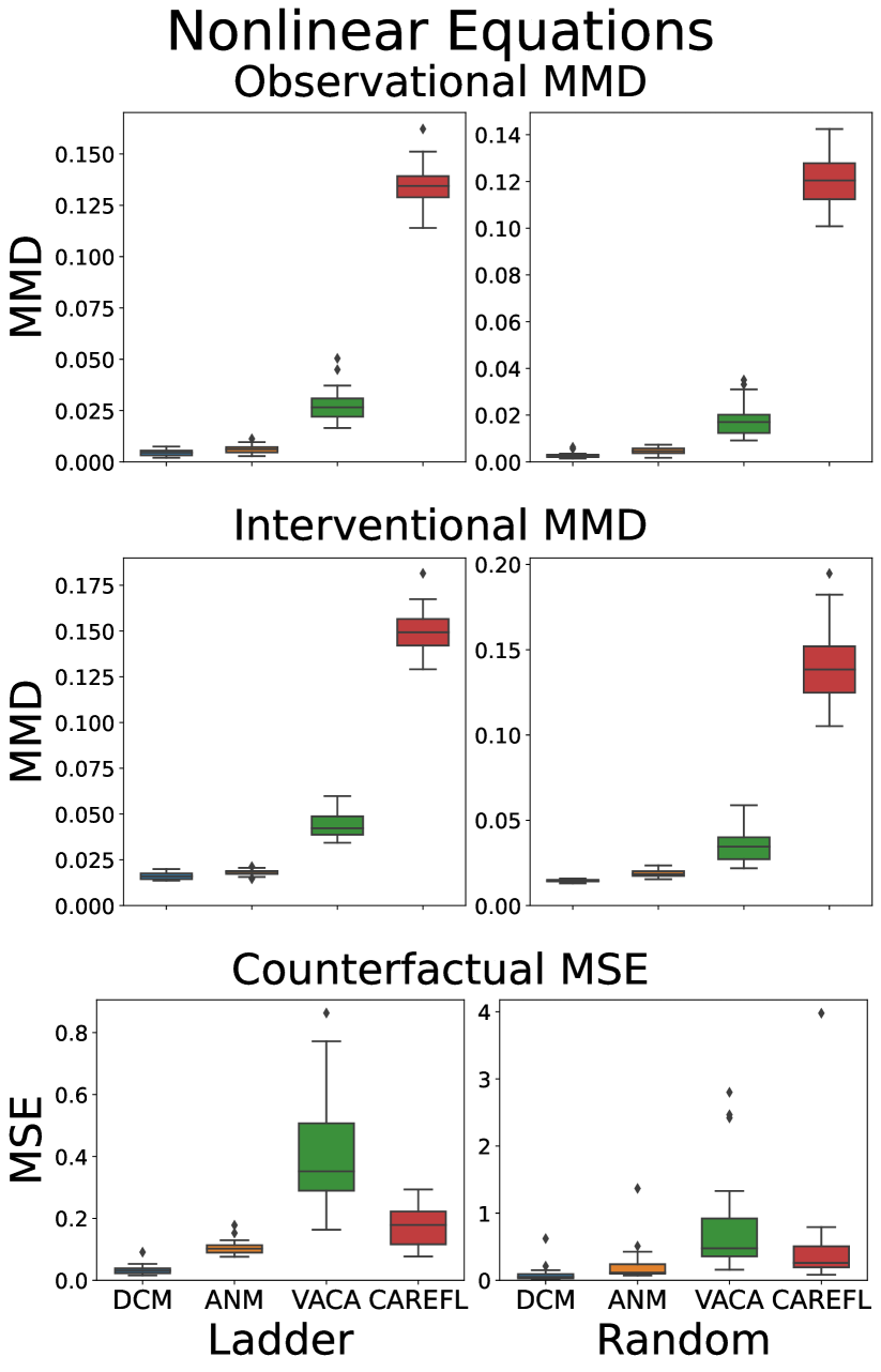
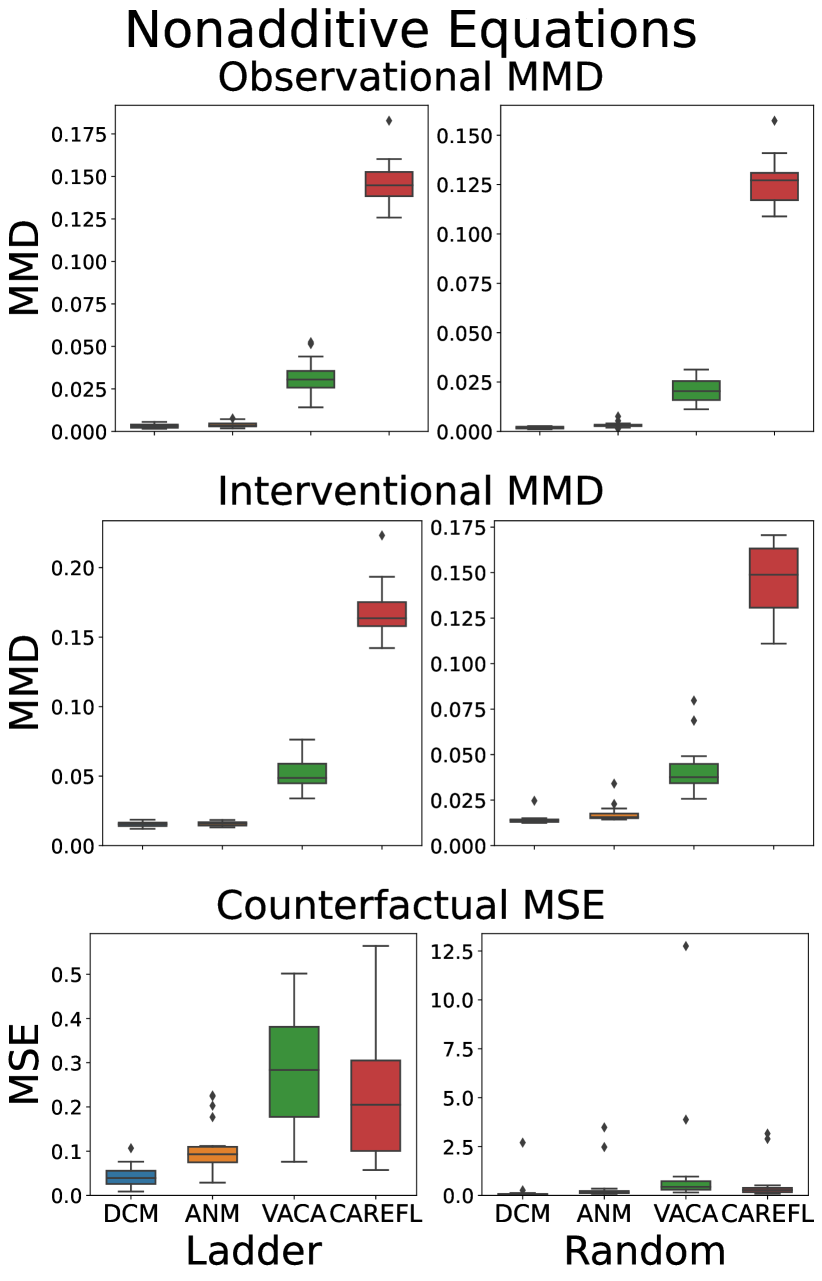
Appendix D Additional Experiments

In this section, we present additional experimental evidence showcasing the superior performance of DCM in addressing various types of causal queries. In Section D.1, we present synthetic data experiments on 3-4 node graph with various common structures. In Section D.2 we provide results on the Sachs graph and dataset from Sachs et al. [2005].

D.1 Additional Synthetic Experiments

In this section, we consider four additional smaller graph structures, which we call the chain, triangle, diamond, and Y graphs (see Figure 3).

The exact equations are presented in Table 4. These functional equations were chosen to balance the signal-to-noise ratio of the covariates and noise to represent realistic settings. Furthermore, these structural equations were chosen after hyperparameter selection, meaning we did not tune DCM’s parameters nor tune the structural equations after observing the performance of the models.

Consider a node with value $X$ with parents $X_{\mathrm{pa}}$ and exogenous noise $U$ where $X_{\mathrm{pa}}\perp\!\!\!\perp U$, and corresponding functional equation $f$ such that

$$X=f(X_{\mathrm{pa}},U).$$

Further assuming the additive noise model, $X:=f_{1}(X_{\mathrm{pa}})+f_{2}(U)$. In this additive setting, since $X_{\mathrm{pa}}\perp\!\!\!\perp U$, we have

$${\textrm{Var}}\,[X]={\textrm{Var}}\,[f_{1}(X_{\mathrm{pa}}]+{\textrm{Var}}\,[f_{2}(U)].$$

We choose $f_{1}$ and $f_{2}$ such that

$$0.05\leq\frac{{\textrm{Var}}\,[f_{2}(U)]}{{\textrm{Var}}\,[f_{1}(X_{\mathrm{pa}}]}\leq 0.5,$$

representing the fact that the ratio of the effect of the noise to the parents is roughly approximate or smaller by an order of magnitude.

For the nonadditive case, we decompose the variance using the law of total variance,

$${\textrm{Var}}\,[X]=\mathbb{E}\,{\textrm{Var}}\,[f(X_{\mathrm{pa}},U)\mid U]+{\textrm{Var}}\,\mathbb{E}[f(X_{\mathrm{pa}},U)\mid U].$$

Similarly, we choose the functional equation $f$ such that $f$ satisfies

$$0.05\leq\frac{{\textrm{Var}}\,\mathbb{E}[f(X_{\mathrm{pa}},U)\mid U]}{\mathbb{E}\,{\textrm{Var}}\,[f(X_{\mathrm{pa}},U)\mid U]}\leq 0.5$$

For all graphs, $U_{i}\overset{\mathrm{iid}}{\sim}\mathcal{N}(0,1)$, and we choose $f$ such that $X_{i}=U_{i}$ if $X_{i}$ is a root node, i.e. $f$ is the identity function. Lastly, we normalize every node $X_{i}$ such that ${\textrm{Var}}\,(X_{i})\approx 1$. For the sake of clarity, we omit all normalizing terms in the formulas and omit functional equations for root nodes below.

Table 4: The equations defining the data generating process in the NLIN and NADD cases.

SCM		Nonlinear Case	Nonadditive Case
Chain	$f_{2}(U_{2},X_{1})$	$\exp(X_{1}/2)+U_{2}/4$	$1/((U_{2}+X_{1})^{2}+0.5)$
	$f_{3}(U_{3},X_{2})$	$(X_{2}-5)^{3}/15+U_{3}$	$\sqrt{X_{2}+\lvert U_{3}\rvert}/(0.1+X_{2})$
Triangle	$f_{2}(U_{2},X_{1})$	$2X_{1}^{2}+U_{2}$	$X_{1}/((U_{2}+X_{1})^{2}+1)+U_{2}/4$
	$f_{3}(U_{3},X_{1},X_{2})$	$20/(1+\exp(-X_{2}^{2}+X_{1}))+U_{3}$	$(\lvert U_{3}\rvert+0.3)(-X_{1}+X_{2}/2+\lvert U_{3}\rvert/5)^{2}$
Diamond	$f_{2}(U_{2},X_{1})$	$X_{1}^{2}+U_{2}/2$	$\sqrt{\lvert X_{1}\rvert}(\lvert U_{2}\rvert+0.1)/2+\lvert X_{1}\rvert+U_{2}/5$
	$f_{3}(U_{3},X_{1},X_{2})$	$X_{2}^{2}-2/(1+\exp(-X_{1}))+U_{3}/2$	$1/(1+(\lvert U_{3}\rvert+0.5)\exp(-X_{2}+X_{1}))$
	$f_{4}(U_{4},X_{2},X_{3})$	$X_{3}/(\lvert X_{2}+2\rvert+X_{3}+0.5)+U_{4}/10$	$(X_{3}+X_{2}+U_{4}/4-7)^{2}-20$
Y	$f_{3}(U_{3},X_{1},X_{2})$	$4/(1+\exp(-X_{1}-X_{2}))-X_{2}^{2}+U_{3}/2$	$(X_{1}-2X_{2}-2)(\lvert U_{3}|+0.2)$
	$f_{4}(U_{4},X_{3})$	$20/(1+\exp(X_{3}^{2}/2-X_{3}))+U_{4}$	$(\cos(X_{3})+U_{4}/2)^{2}$

Results. For these 4 graph structures (chain, triangle, diamond, and Y), in Table 5, we provide the performance of all evaluated models for observational, interventional, and counterfactual queries, averaged over $10$ separate initializations of models and training data, with the lowest value in each row bolded. The values are multiplied by $100$ for clarity. In Figure 2, we show the box plots for the same set of experiments.

The results here are similar to those observed with the larger graph structures in Table 1. DCM has the lowest error in 7 out of 12 of the nonlinear settings, with the correctly specified ANM having the lowest error in the remaining 5. Furthermore, DCM and ANM both typically have a lower standard deviation compared to the other competing methods. For the nonadditive settings, DCM demonstrates the lowest values for all 12 causal queries.

Table 5: Mean$\pm$standard deviation of observational, interventional, and counterfactual queries of four different SCMs in nonlinear and nonadditive settings over $10$ random initializations of the model and training data. The values are multiplied by $100$ for clarity.

			DCM	ANM	VACA	CAREFL
SCM		Metric	($\times 10^{-2}$)	($\times 10^{-2}$)	($\times 10^{-2}$)	($\times 10^{-2}$)
Chain	NLIN	Obs. MMD	0.27$\pm$0.11	0.19$\pm$0.27	1.63$\pm$0.42	4.25$\pm$1.12
		Int. MMD	1.71$\pm$0.27	1.70$\pm$0.47	10.10$\pm$1.81	8.63$\pm$0.52
		CF. MSE	0.33$\pm$0.16	2.43$\pm$2.49	25.99$\pm$6.47	19.62$\pm$4.01
	NADD	Obs. MMD	0.22$\pm$0.16	1.51$\pm$0.43	1.53$\pm$0.41	3.48$\pm$1.06
		Int. MMD	2.85$\pm$0.45	7.34$\pm$0.62	10.42$\pm$2.77	11.02$\pm$1.32
		CF. MSE	75.84$\pm$1.65	88.56$\pm$2.63	98.82$\pm$4.16	105.80$\pm$11.04
Triangle	NLIN	Obs. MMD	0.16$\pm$0.11	0.12$\pm$0.07	3.12$\pm$0.93	4.64$\pm$1.03
		Int. MMD	1.50$\pm$0.30	3.28$\pm$0.79	18.43$\pm$1.72	7.08$\pm$0.82
		CF. MSE	1.12$\pm$0.26	9.80$\pm$1.70	178.69$\pm$16.45	41.85$\pm$19.58
	NADD	Obs. MMD	0.25$\pm$0.12	0.51$\pm$0.08	2.42$\pm$0.48	5.12$\pm$1.10
		Int. MMD	2.81$\pm$0.21	5.54$\pm$0.60	11.09$\pm$0.85	4.17$\pm$0.44
		CF. MSE	26.28$\pm$6.68	97.25$\pm$16.45	173.67$\pm$16.28	121.99$\pm$31.34
Y	NLIN	Obs. MMD	0.11$\pm$0.05	0.14$\pm$0.08	2.29$\pm$0.69	6.82$\pm$0.85
		Int. MMD	1.23$\pm$0.08	1.40$\pm$0.14	9.50$\pm$0.96	14.97$\pm$1.29
		CF. MSE	0.28$\pm$0.25	1.22$\pm$0.27	28.79$\pm$4.02	27.85$\pm$5.33
	NADD	Obs. MMD	0.21$\pm$0.15	1.00$\pm$0.19	1.51$\pm$0.44	3.39$\pm$0.58
		Int. MMD	1.54$\pm$0.23	5.62$\pm$0.31	5.37$\pm$0.72	6.51$\pm$0.40
		CF. MSE	33.45$\pm$2.06	47.55$\pm$2.56	60.67$\pm$3.24	52.41$\pm$6.69
Diamond	NLIN	Obs. MMD	0.22$\pm$0.10	0.13$\pm$0.07	2.77$\pm$0.45	8.28$\pm$1.29
		Int. MMD	3.21$\pm$0.62	2.56$\pm$0.31	25.30$\pm$1.39	18.23$\pm$3.01
		CF. MSE	14.74$\pm$6.09	32.02$\pm$37.74	138.65$\pm$12.33	607.62$\pm$241.21
	NADD	Obs. MMD	0.25$\pm$0.18	0.28$\pm$0.09	2.36$\pm$0.44	5.50$\pm$0.81
		Int. MMD	1.88$\pm$0.23	4.40$\pm$0.52	12.54$\pm$0.89	16.34$\pm$1.72
		CF. MSE	1.36$\pm$0.14	8.58$\pm$0.77	57.40$\pm$4.23	24.61$\pm$7.05

Figure 2: Top: Nonlinear setting (NLIN), Bottom: Nonadditive setting (NADD). Box plots of observational, interventional, and counterfactual queries of four different SCMs over $10$ random initializations of the model and training data.

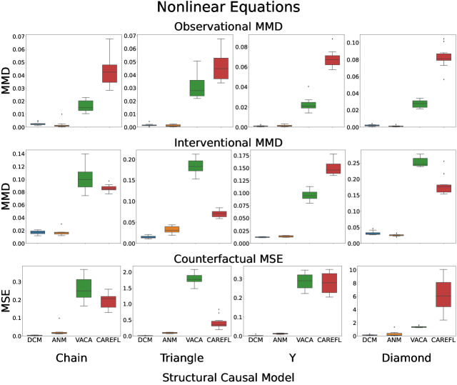
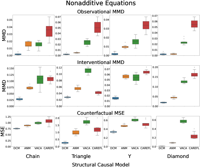
(a) Ladder graph.

(b) Example of a random graph, used in Section 5, with exogenous noise nodes omitted for clarity.

(c) Chain graph.

(d) Triangle graph.

(e) Diamond graph.

(f) Y graph.

Figure 3: Causal graphs used in our experiments.

D.2 Semi-Synthetic Experiments

To further evaluate the effectiveness of DCM, we explore a semi-synthetic experiment based on the Sachs dataset [Sachs et al., 2005]. We use the real world graph from comprised of 11 nodes. The graph represents an intricate network of signaling pathways within human T cells. The 11 nodes within this graph each correspond to one of the phosphorylated proteins or phospholipids that were examined in their study.

For our experiment, we sample data in a semi-synthetic manner. For the root nodes, we sample from the empirical marginal distribution. For non-root nodes, since the ground truth structural equations are unknown, we use a random neural network as the structural equation, as was done in Section 5. We report the performances in Table 6. We see that the performance improvements with our DCM approach corroborate our prior findings.

Table 6: Mean$\pm$standard deviation of observational, interventional, and counterfactual queries of the Sachs SCM in nonlinear (NLIN) and nonadditive (NADD) settings over $10$ random initializations of the model and training data. The values are multiplied by $100$ for clarity.

			DCM	ANM	VACA	CAREFL
SCM		Metric	($\times 10^{-2}$)	($\times 10^{-2}$)	($\times 10^{-2}$)	($\times 10^{-2}$)
Sachs	NLIN	Obs. MMD	0.31$\pm$0.15	0.21$\pm$0.04	0.53$\pm$0.24	7.30$\pm$0.95
		Int. MMD	1.25$\pm$0.11	1.37$\pm$0.12	2.03$\pm$0.36	5.77$\pm$0.85
		CF. MSE	0.72$\pm$0.19	4.72$\pm$1.71	17.71$\pm$9.23	9.59$\pm$2.52
	NADD	Obs. MMD	0.18$\pm$0.07	0.18$\pm$0.06	0.39$\pm$0.24	6.10$\pm$1.14
		Int. MMD	1.42$\pm$0.26	1.86$\pm$0.51	2.21$\pm$0.98	5.29$\pm$2.07
		CF. MSE	1.99$\pm$2.49	4.68$\pm$5.77	7.30$\pm$11.57	8.30$\pm$8.34

References

- Alaa and Van Der Schaar (2017) Ahmed M Alaa and Mihaela Van Der Schaar. Bayesian inference of individualized treatment effects using multi-task gaussian processes. Advances in neural information processing systems, 30, 2017.
- Blair (2000) David E Blair. Inversion theory and conformal mapping, volume 9. American Mathematical Soc., 2000.
- Blöbaum et al. (2022) Patrick Blöbaum, Peter Götz, Kailash Budhathoki, Atalanti A. Mastakouri, and Dominik Janzing. Dowhy-gcm: An extension of dowhy for causal inference in graphical causal models. arXiv preprint arXiv:2206.06821, 2022.
- Deng et al. (2009) Jia Deng, Wei Dong, Richard Socher, Li-Jia Li, Kai Li, and Li Fei-Fei. Imagenet: A large-scale hierarchical image database. In 2009 IEEE Conference on Computer Vision and Pattern Recognition, pages 248–255, 2009. doi: 10.1109/CVPR.2009.5206848.
- Dhariwal and Nichol (2021) Prafulla Dhariwal and Alexander Nichol. Diffusion models beat gans on image synthesis. In M. Ranzato, A. Beygelzimer, Y. Dauphin, P.S. Liang, and J. Wortman Vaughan, editors, Advances in Neural Information Processing Systems, volume 34, pages 8780–8794. Curran Associates, Inc., 2021. URL https://proceedings.neurips.cc/paper/2021/file/49ad23d1ec9fa4bd8d77d02681df5cfa-Paper.pdf.
- Durkan et al. (2019) Conor Durkan, Artur Bekasov, Iain Murray, and George Papamakarios. Neural spline flows. In H. Wallach, H. Larochelle, A. Beygelzimer, F. d'Alché-Buc, E. Fox, and R. Garnett, editors, Advances in Neural Information Processing Systems, volume 32. Curran Associates, Inc., 2019. URL https://proceedings.neurips.cc/paper/2019/file/7ac71d433f282034e088473244df8c02-Paper.pdf.
- Elfwing et al. (2018) Stefan Elfwing, Eiji Uchibe, and Kenji Doya. Sigmoid-weighted linear units for neural network function approximation in reinforcement learning. Neural Networks, 107:3–11, 2018. ISSN 0893-6080. doi: https://doi.org/10.1016/j.neunet.2017.12.012. URL https://www.sciencedirect.com/science/article/pii/S0893608017302976. Special issue on deep reinforcement learning.
- Garrido et al. (2021) Sergio Garrido, Stanislav Borysov, Jeppe Rich, and Francisco Pereira. Estimating causal effects with the neural autoregressive density estimator. Journal of Causal Inference, 9(1):211–218, 2021.
- Gretton et al. (2007) Arthur Gretton, Kenji Fukumizu, Choon Teo, Le Song, Bernhard Schölkopf, and Alex Smola. A kernel statistical test of independence. In J. Platt, D. Koller, Y. Singer, and S. Roweis, editors, Advances in Neural Information Processing Systems, volume 20. Curran Associates, Inc., 2007. URL https://proceedings.neurips.cc/paper/2007/file/d5cfead94f5350c12c322b5b664544c1-Paper.pdf.
- Gretton et al. (2012) Arthur Gretton, Karsten M. Borgwardt, Malte J. Rasch, Bernhard Schölkopf, and Alexander Smola. A kernel two-sample test. Journal of Machine Learning Research, 13(25):723–773, 2012. URL http://jmlr.org/papers/v13/gretton12a.html.
- Ho and Salimans (2021) Jonathan Ho and Tim Salimans. Classifier-free diffusion guidance. In NeurIPS 2021 Workshop on Deep Generative Models and Downstream Applications, 2021. URL https://openreview.net/forum?id=qw8AKxfYbI.
- Ho et al. (2020) Jonathan Ho, Ajay Jain, and Pieter Abbeel. Denoising diffusion probabilistic models. In H. Larochelle, M. Ranzato, R. Hadsell, M.F. Balcan, and H. Lin, editors, Advances in Neural Information Processing Systems, volume 33, pages 6840–6851. Curran Associates, Inc., 2020. URL https://proceedings.neurips.cc/paper/2020/file/4c5bcfec8584af0d967f1ab10179ca4b-Paper.pdf.
- Hoyer et al. (2008) Patrik Hoyer, Dominik Janzing, Joris M Mooij, Jonas Peters, and Bernhard Schölkopf. Nonlinear causal discovery with additive noise models. Advances in neural information processing systems, 21, 2008.
- Karimi et al. (2020) Amir-Hossein Karimi, Julius Von Kügelgen, Bernhard Schölkopf, and Isabel Valera. Algorithmic recourse under imperfect causal knowledge: a probabilistic approach. Advances in neural information processing systems, 33:265–277, 2020.
- Khemakhem et al. (2021) Ilyes Khemakhem, Ricardo Monti, Robert Leech, and Aapo Hyvarinen. Causal autoregressive flows. In Arindam Banerjee and Kenji Fukumizu, editors, Proceedings of The 24th International Conference on Artificial Intelligence and Statistics, volume 130 of Proceedings of Machine Learning Research, pages 3520–3528. PMLR, 13–15 Apr 2021. URL https://proceedings.mlr.press/v130/khemakhem21a.html.
- Kocaoglu et al. (2018) Murat Kocaoglu, Christopher Snyder, Alexandros G Dimakis, and Sriram Vishwanath. Causalgan: Learning causal implicit generative models with adversarial training. In International Conference on Learning Representations, 2018.
- Kong et al. (2021) Zhifeng Kong, Wei Ping, Jiaji Huang, Kexin Zhao, and Bryan Catanzaro. Diffwave: A versatile diffusion model for audio synthesis. In International Conference on Learning Representations, 2021. URL https://openreview.net/forum?id=a-xFK8Ymz5J.
- Lu et al. (2020) Chaochao Lu, Biwei Huang, Ke Wang, José Miguel Hernández-Lobato, Kun Zhang, and Bernhard Schölkopf. Sample-efficient reinforcement learning via counterfactual-based data augmentation. arXiv preprint arXiv:2012.09092, 2020.
- Moraffah et al. (2020) Raha Moraffah, Bahman Moraffah, Mansooreh Karami, Adrienne Raglin, and Huan Liu. Can: A causal adversarial network for learning observational and interventional distributions. arXiv preprint arXiv:2008.11376, 2020.
- Muandet et al. (2021) Krikamol Muandet, Motonobu Kanagawa, Sorawit Saengkyongam, and Sanparith Marukatat. Counterfactual mean embeddings. J. Mach. Learn. Res., 22:162–1, 2021.
- Nasr-Esfahany and Kiciman (2023) Arash Nasr-Esfahany and Emre Kiciman. Counterfactual (non-) identifiability of learned structural causal models. arXiv preprint arXiv:2301.09031, 2023.
- Nasr-Esfahany et al. (2023) Arash Nasr-Esfahany, Mohammad Alizadeh, and Devavrat Shah. Counterfactual identifiability of bijective causal models. arXiv preprint arXiv:2302.02228, 2023.
- Nichol and Dhariwal (2021) Alexander Quinn Nichol and Prafulla Dhariwal. Improved denoising diffusion probabilistic models. In Marina Meila and Tong Zhang, editors, Proceedings of the 38th International Conference on Machine Learning, volume 139 of Proceedings of Machine Learning Research, pages 8162–8171. PMLR, 18–24 Jul 2021. URL https://proceedings.mlr.press/v139/nichol21a.html.
- Parafita and Vitrià (2020) Álvaro Parafita and Jordi Vitrià. Causal inference with deep causal graphs. arXiv preprint arXiv:2006.08380, 2020.
- Pawlowski et al. (2020) Nick Pawlowski, Daniel Coelho de Castro, and Ben Glocker. Deep structural causal models for tractable counterfactual inference. Advances in Neural Information Processing Systems, 33:857–869, 2020.
- Pearl et al. (2016) J. Pearl, M. Glymour, and N.P. Jewell. Causal Inference in Statistics: A Primer. Wiley, 2016. ISBN 9781119186847. URL https://books.google.com/books?id=L3G-CgAAQBAJ.
- Pearl (2009a) Judea Pearl. Causal inference in statistics: An overview. Statistics Surveys, 3(none):96 – 146, 2009a. doi: 10.1214/09-SS057. URL https://doi.org/10.1214/09-SS057.
- Pearl (2009b) Judea Pearl. Causal inference in statistics: An overview. 2009b.
- Ramesh et al. (2022) Aditya Ramesh, Prafulla Dhariwal, Alex Nichol, Casey Chu, and Mark Chen. Hierarchical text-conditional image generation with clip latents. 2022. URL https://arxiv.org/abs/2204.06125.
- Sachs et al. (2005) Karen Sachs, Omar Perez, Dana Pe’er, Douglas A. Lauffenburger, and Garry P. Nolan. Causal protein-signaling networks derived from multiparameter single-cell data. Science, 308(5721):523–529, 2005. doi: 10.1126/science.1105809. URL https://www.science.org/doi/abs/10.1126/science.1105809.
- Saha and Garain (2022) Saptarshi Saha and Utpal Garain. On noise abduction for answering counterfactual queries: A practical outlook. Transactions on Machine Learning Research, 2022.
- Saharia et al. (2022) Chitwan Saharia, William Chan, Saurabh Saxena, Lala Li, Jay Whang, Emily Denton, Seyed Kamyar Seyed Ghasemipour, Burcu Karagol Ayan, S. Sara Mahdavi, Rapha Gontijo Lopes, Tim Salimans, Jonathan Ho, David J Fleet, and Mohammad Norouzi. Photorealistic text-to-image diffusion models with deep language understanding. 2022. URL https://arxiv.org/abs/2205.11487.