Dynamic Atomic Column Detection in Transmission Electron Microscopy Videos via Ridge Estimation

Abstract

Ridge detection is a classical tool to extract curvilinear features in image processing. As such, it has great promise in applications to material science problems; specifically, for trend filtering relatively stable atom-shaped objects in image sequences, such as Transmission Electron Microscopy (TEM) videos. Standard analysis of TEM videos is limited to frame-by-frame object recognition. We instead harness temporal correlation across frames through simultaneous analysis of long image sequences, specified as a spatio-temporal image tensor. We define new ridge detection algorithms to non-parametrically estimate explicit trajectories of atomic-level object locations as a continuous function of time. Our approach is specially tailored to handle temporal analysis of objects that seemingly stochastically disappear and subsequently reappear throughout a sequence. We demonstrate that the proposed method is highly effective and efficient in simulation scenarios, and delivers notable performance improvements in TEM experiments compared to other material science benchmarks.

, , label=e3]crozier@asu.edu, and

1 Introduction

Transmission electron microscopy (TEM) is an essential tool for studying materials at the atomic level. Major technical advancements in TEM have improved not only temporal resolution but also sensitivity for atomic structure detection (Ruskin, Yu and Grigorieff, 2013; Faruqi and McMullan, 2018; Levin, 2021). TEM images are known to suffer critical degradation in signal-to-noise ratios (SNR) (Lawrence et al., 2020, 2021; Vincent and Crozier, 2021) due to the scientific demands for instantaneous analysis coupled with the limited equipment capacity of electron flux (Egerton, Li and Malac, 2004; Egerton, 2013, 2019). Section 1 is an illustration of a real TEM video with high temporal resolution, where the severe SNR challenge can be read from the example frame. Hence, improved analysis algorithms for TEM images and videos are in continuous demand, and incubated at varied focus and strength (Lawrence et al., 2020). Yet, important weaknesses still remain and accompanying data-intensive methodology is urgently needed.

In analysis of gray-scale TEM images, the most essential task is to estimate (detect) nanoparticle structure and summarize (extract) important atomic features to quantify and understand physical atomic dynamics, especially for in situ experiments with catalysts. Fitting Gaussian models is the classical benchmark method and enjoys its popularity due to its straightforward interpretations. This requires various estimation routines including nonlinear least-square Gaussian Peak Fitting (GPF, Levin, Lawrence and Crozier 2020) and Atomap (AM, Nord et al. 2017). However, it is restrictive in terms of elliptical shape assumptions, and it is extremely computationally sensitive to both initialization as well as the SNR conditions. Manzorro et al. (2022) recently introduced a blob detection (BD) approach tailored for TEM images. Their algorithm drops the explicit shape constraints and copes with the severe SNR challenge. Meanwhile, limitations remain, especially when methods are also needed to distinguish absence of atomic columns from vacuum background. (Thomas et al., 2022) proposed a topological data analysis (TDA) method to verify such differences using a hypothesis testing schema. The algorithm also requires less restrictive graphical assumptions. Some machine learning algorithms (e.g., Lin et al. 2021) have also been developed, but the models therein are usually trained given very narrow SNR levels and current use cases lack generalizability.

The sketch of a time-resolved in situ TEM video of a $\mbox{CeO}_{2}$ nanoparticle with temporal resolution 2.5 milliseconds. Here, the $x$ and $y$ axes identify the spatial coordinates within single TEM image frames, and the $t$ axis represents the dimension of time. Every single frame visualizes the physical nanoparticles’ model as the gray-scaled projection image, and the whiter regions are the places where atoms are stacked to form atomic columns perpendicular to the page. A zoomed view for one of the atomic columns is provided as Section 1.[.5] The illustration of a generalized ridge curve $\gamma\subset\mathbb{R}^{3}$ as a trajectory function of time $t$ for a selected atomic column after negating the TEM video. The negation is supported as in Remark 1. In the example sequence, the atomic column experiences various dynamics such as shrinking and expanding radius, decreasing and increasing contrasts, and total degeneration to a single point in the middle of the series. In addition, the outer contour of the atomic column forms a tube-shaped object that stretches temporally. [.45]

Since most of these analyses have limited focus on individual frames, the assumptions ranging from graphical shapes to nanoparticles’ intact lattice structures are usually necessary. Meanwhile these assumptions may frequently be violated in real experiments due to the atoms’ volatile movements. On the other hand, the raw TEM data do not seem to be fully exploited. In this paper, we introduce a novel point of view on the spatio-temporal TEM image tensor (Section 1), and propose a generalized ridge detection (RD) algorithm that makes use of the rarely accounted for temporal correlation. Our ridge formulation is naturally motivated and justified by stacking the same atomic column’s BD output blobs temporally to form a tube; see Section 1. Note that such tubes in raw TEM videos usually correspond to valleys instead of ridges as the pixel intensities of atomic columns have smaller values than those of neighboring regions according to TEM mechanisms, hence negation is needed prior to our ridge processing.

Some of the existing milestone algorithms may utilize the TEM history only for denoising purposes during preprocessing. Our proposed ridge detection approach treats such information differently. It not only employs the data structure more profoundly to interpolate the curved cylinder of temporally-piled atomic columns, but also maintains sufficient independence between frames instead of completely smoothing out local features.

Regarding image processing, Lindeberg (1996) first introduced the scale-space detection operator to adaptively account for lines’ width. Since then, some state-of-art methodologies of ridge detection have been developed, such as meijering (Meijering et al., 2004), sato (Sato et al., 1998), frangi (Frangi et al., 1998), and hessian (Ng et al., 2015). Indeed, these algorithms reassign each pixel with a score of it being on a ridge, and reproduce the image with denoised and intensified curvilinear patterns. The image processing python package scikit-image (van der Walt et al., 2014) offers a collection of the above four implementations. Subsequent works proposed different types of filtering measures and/or threshold schema with various tools. For example, Norgard and Bremer (2013) introduced the combinatorial Jacobi sets to guarantee valid global structures, Lopez-Molina et al. (2015) used the Anisotropic Gaussian Kernel (AGK) to improve sensitivity and robustness, and Reisenhofer and King (2019) combined the contrast-invariant phase congruency measure with $\alpha$-molecules to refine local features given limited samples. For comprehensive reviews on ridge detection and enhancement algorithms, see Shokouh et al. (2021); Alhasson et al. (2021), and references therein. Ridge detection has many applications including medical images analysis (Lopez et al., 1999), fingerprint enhancement (Lindeberg and Almansa, 2000), autonomous navigation (Beyeler, Mirus and Verl, 2014), signal processing (Colominas, Meignen and Pham, 2020; Laurent and Meignen, 2022), and geology (Pham et al., 2021), to name a few.

The related Lagrangian coherent structures (LCSs, Haller and Yuan 2000; Haller 2002) methods are regarded as a ridge variant in mechanical engineering and dynamic systems (Mathur et al., 2007; Senatore and Ross, 2011; Schindler et al., 2012); they aim to separate different fluid behaviors in finite-time Lyapunov exponent fields (Kasten et al., 2009). Computationally, they are usually filtered using numerical differential equation solvers; see Ameli, Desai and Shadden (2014) for examples.

Overall, the primary focus of the image processing community has been establishing filtered pixel-wise ridge-likelihood images for enhanced visual inspection, while the mechanical engineering community focuses its efforts on approximating ridges using discretized numerical solvers. Hence, analytical tools with the combination of ridge detection and continuous characterization are needed. The breakthrough of this work is to introduce innovative methodology to non-parametrically extract the continuous trajectories of atomic columns in TEM videos, with the tolerance of occasional degeneration throughout the sequence. In practice, we refer to the idea in some existing methods (Levin, Lawrence and Crozier, 2020; Manzorro et al., 2022), and propose to process one atomic column at a time. The algorithm focuses on the cropped videos which spatially correspond to the approximate regions of atomic columns, and outputs one single ridge curve after every run. Given the data’s discrete nature, diverse trajectory curvatures and the potential degeneration, our investigation with anticipated continuous output is challenging and novel.

This paper is organized as follows. Section 2 introduces preliminaries including notations, necessary setup assumptions, and preprocessing steps. The details of our methodology are introduced in Section 3. Section 4 delivers some elementary and discrete results for uncertainty summaries about an estimated curve. Supported by simulated results from Section 5, Section 6 demonstrates the superior performance of our method in our motivating TEM application (above) in material science. Section 7 concludes with discussion. Appendix A introduces an optional alternative schema of methodology development that supplements and partially updates Section 3. Proofs for selected propositions from throughout the paper appear in Appendix B.

2 Preliminaries

Throughout this paper, a video is described by a sequence (length $T$) of gray-scale images, each with size $M\times N$. The set of pixel indices is given by the collection $\Omega=\{(m,n,\tau):m\in[M];n\in[N];\tau\in[T]\}$ where we introduce the notation $[k]=\{0,1,\dots,k-1\}$ for integer $k$. In addition, for $\tau\in[T]$, we denote the $t=\tau$ image frame as $\Omega(\tau)=\Omega\bigcap\{(x,y,t):t=\tau\}$.

The pixel values of the image sequence are discretely evaluated by a mapping $f(x,y,t):\mathbb{R}^{3}\to\mathbb{R}$ at the triplet grid locations $(x,y,t)=(m,n,\tau)\in\Omega$, denoted as $f_{m,n,\tau}$. A continuous ridge curve, which may not be restricted to the lattice $\Omega$, is defined as $\gamma:\mathbb{R}\to\mathbb{R}^{3}$.

Denote $e_{t}$ as the indicator vector for the temporal dimension, i.e., $e_{t}=(0,0,1)$. For a matrix $A$, $\operatorname{tr}(A)$ represents the trace and $A^{+}$ denotes its Moore-Penrose general inverse. The operator $x_{+}$ computes $\max(x,0)$ for any scalar $x$. For two vectors $a$ and $b$ of the same dimension, we denote $\big{<}a,b\big{>}$ as their dot product, and $\cos(a,b)=\frac{\langle a,b\rangle}{\|a\|\cdot\|b\|}$ as the cosine similarity between them. The indicator function $\mathbbm{1}(X)$ takes value 1 (or 0) if the statement $X$ is true (or false).

We define a ridge $\gamma$ as a continuous collection of points on a three-dimensional mapping $f$ which graphically resembles the tube-shaped object as demonstrated in Section 1. Here the definition gets slightly extended from some other similar alternatives (e.g., Porteous 2001), see Condition 2 below, to allow for degenerate eigenvalues. In consequence, the trajectory curve in our TEM application will not get suspended at those extraordinary image frames when the atomic column is absent.

Definition 1.

Given a second-order differentiable mapping $f:\mathbb{R}^{3}\to\mathbb{R}$, denote $\nabla_{f}(p)\in\mathbb{R}^{3}$ and $\Delta_{f}(p)\in\mathbb{R}^{3\times 3}$ as the gradient vector and the Hessian matrix of the mapping $f$ at point $p\in\mathbb{R}^{3}$, respectively. Additionally, assume the Hessian matrix $\Delta_{f}(p)$ has eigenvalues $\lambda_{f,1}(p),\lambda_{f,2}(p),\lambda_{f,3}(p)$ and corresponding unit eigenvectors $v_{f,1}(p),v_{f,2}(p),v_{f,3}(p)\in\mathbb{R}^{3}$. Then, $p$ is a point on a ridge of $f$, denoted by $\gamma\subset\mathbb{R}^{3}$, if

1. $\big{<}\nabla_{f}(p),v_{f,2}(p)\big{>}=\big{<}\nabla_{f}(p),v_{f,3}(p)\big{>}=0$, i.e., the gradient $\nabla_{f}(p)$ is parallel to the Hessian eigenvector $v_{f,1}(p)$. Consequently, the tangent direction of the ridge $\gamma$ at $p$ is characterized by $v_{f,1}(p)$;

2. $0\geq\lambda_{f,2}(p)\geq\lambda_{f,3}(p)$;

3. Furthermore, the curvature of the mapping $f$ along direction $v_{f,1}(p)$ is small or relatively small, i.e., $|\lambda_{f,i}(p)|\gg|\lambda_{f,1}(p)|$ or $\left|\frac{\lambda_{f,i}(p)}{\lambda_{f,1}(p)}\right|\gg 1$ for both $i=2$ and $3$, where $\gg$ denotes much greater than.

Remark 1.

1. The Figure 1 graphically illustrates Definition 1. Generally speaking, if we introduce at point $p$ a local coordinate system different from the classical Cartesian $(x,y,t)$ representations, and specify the axes using the local Hessian eigenvectors $\{v_{f,1}(p),v_{f,2}(p),v_{f,3}(p)\}$, then $p$ is on a ridge if the mapping $f$ attains the local maximum at $p$ along two of the three axes directions; see the latter two subplots in Figure 1. In the TEM video application, these two axes form the plane that is usually close to the image frame.

2. The definition of valleys only differs from Definition 1 in Condition 2 with all the inequality signs flipped, i.e., a ridge point $p$ of the mapping $f$ is naturally a valley point of $-f$. With the shift- and scale-free properties imposed through later development, our method can directly take the negated TEM video as the input for implementation.

3. In our later analysis, especially when concerning the TEM application, the video mapping $f$ is characterized by the discrete pixel values and remains fixed. We will omit the subscript $f$ for conciseness.

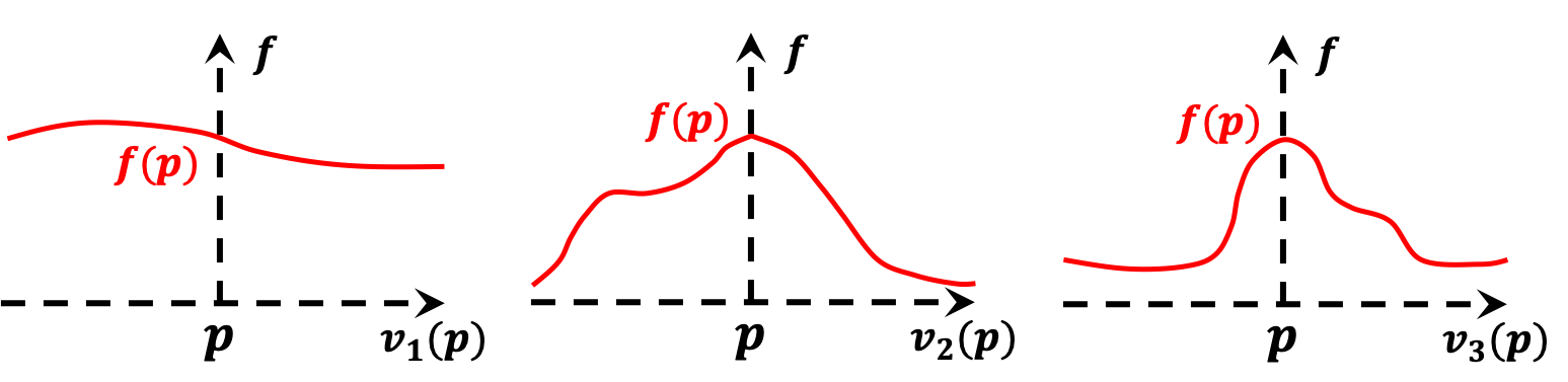
Figure 1: The projected behaviors of the mapping $f$ at a ridge point $p\in\gamma$ along the axes of a local coordinate system. Here the basis of the new coordinate system is formed by the set of orthonormal Hessian eigenvectors $\{v_{1}(p),v_{2}(p),v_{3}(p)\}$.

We then impose an essential setup assumption to fix the temporal axis as the major stretch direction of the ridge $\gamma$.

Assumption 1.

There exists one unique continuous ridge curve $\gamma$ within the video region $[0,M)\times[0,N)\times[0,T)$ that can be parameterized temporally, i.e., $\forall t\in[0,T)$, there exists one unique ridge mapping

$$\gamma(t)=(u(t),w(t),t)\in[0,M)\times[0,N)\times[0,T),$$ (1)

where $u(t)$ and $w(t)$ are corresponding spatial coordinates functions. Furthermore, the ridge has tangent $\gamma^{\prime}(t)=(u^{\prime}(t),w^{\prime}(t),1)$.

Remark 2.

In Assumption 1, we impose the existence and uniqueness restrictions, as they comply with our proposed TEM application which processes one atomic column at a time given the cropped TEM videos. The parameterization (1) is motivated by the application on TEM videos, where like Section 1, the spheres of the atomic columns from the TEM video are stacked relatively stably across time to form a tube. In addition, (1) is beneficiary for follow-up analysis. For example, given the input of any frame index $\tau\in[T]$, the ridge function $\gamma$ can then directly return the corresponding spatial location of the selected atomic column within the specific frame.

The computation of first- and second-order derivatives are essential in Definition 1, especially with the discrete nature of the pixel lattice $\Omega$. We propose to convolve with Gaussian functions not only to smooth the noisy data but also to give better behaved differentials.

Definition 2.

Denote the three-dimensional Gaussian function

$$G(x,y,t;\sigma,\delta)=\frac{1}{2\pi\sigma^{2}\cdot\sqrt{2\pi\delta^{2}}}\exp(-\frac{x^{2}+y^{2}}{2\sigma^{2}}-\frac{t^{2}}{2\delta^{2}}),$$

where $\sigma$ and $\delta$ represent spatial and temporal scales, respectively. Then, given $p\in\Omega$, the scaled gradient vector and Hessian matrix

$$\widetilde{\nabla}(p)=(\sigma\widetilde{\nabla}_{x}(p),\sigma\widetilde{\nabla}_{y}(p),\delta\widetilde{\nabla}_{t}(p))^{\prime}\quad\mbox{\&}\quad\widetilde{\Delta}(p)=\begin{pmatrix}\sigma^{2}\widetilde{\Delta}_{xx}(p)&\sigma^{2}\widetilde{\Delta}_{xy}(p)&\sigma\delta\widetilde{\Delta}_{xt}(p)\\ \sigma^{2}\widetilde{\Delta}_{yx}(p)&\sigma^{2}\widetilde{\Delta}_{yy}(p)&\sigma\delta\widetilde{\Delta}_{yt}(p)\\ \sigma\delta\widetilde{\Delta}_{tx}(p)&\sigma\delta\widetilde{\Delta}_{ty}(p)&\delta^{2}\widetilde{\Delta}_{tt}(p)\end{pmatrix}$$ (2)

of the mapping $f$ are approximated by evaluating the elements of partial derivatives via discrete convolutions analogous to

$$\widetilde{\nabla}_{x}(p) =\frac{\partial}{\partial x}\Big{(}\sum_{(m,n,\tau)\in\Omega}f_{m,n,\tau}G(x-m,y-n,t-\tau;\sigma,\delta)\Big{)}_{(x,y,t)=p},$$

$$\widetilde{\Delta}_{xx}(p) =\frac{\partial^{2}}{\partial x^{2}}\Big{(}\sum_{(m,n,\tau)\in\Omega}f_{m,n,\tau}G(x-m,y-n,t-\tau;\sigma,\delta)\Big{)}_{(x,y,t)=p}.$$

Remark 3.

Though both multiplied in the scale-space derivatives (2) (Lindeberg, 1998), the scale $\delta$ along the temporal axis merely serves as the denoising parameter through convolution, while its spatial counterpart $\sigma$ plays its additional role for automatic scale adaptation (Lindeberg, 1996). In practice, the spatial scale $\sigma$ usually implies the size of the atomic column in the TEM images, and is tuned with references from the cross-sectional radii of the tube-shaped object as in Section 1. On the other hand, the temporal scale $\delta$ is often set small to preserve as much subtle dynamics as possible to accurately recover the ridge’s local curvatures, which correspond to the minor movements of the interested atomic column in the TEM application.

Assumption 2.

The gradient vectors $\widetilde{\nabla}(p)$ are non-singular.

Remark 4.

Assumption 2 is imposed to avoid singular derivatives in computation. It is not restrictive, given the noise of the image dataset and the convolution applied in preprocessing. It only restricts the estimators with noise present hence does not rule out the possibilities of those underlying singular cases that we aim to tackle.

The next definition standardizes and updates the estimated Hessian matrix $\widetilde{\Delta}(p)$ in order to improve the universal applicability of our method.

Definition 3.

Set $\mu$ as the median of the gradients norms $\{\|\widetilde{\nabla}(p)\|:p\in\Omega\}$. The Hessian matrices are updated by

$$\widetilde{\Delta}(p)\mapsto\widetilde{\Delta}(p)/\mu.$$ (3)

Remark 5.

1. The update (3) for the Hessian matrices is introduced to ensure the scale-free property of our approach, so that the developed algorithm can be universally implemented on various image sequences with different levels of pixel intensities.

2. For simplicity hereafter, the Hessian $\Delta(p)$ and its approximation $\widetilde{\Delta}(p)$ in (3) will share the same notations of eigenvalues $\lambda_{i}(p)$ and eigenvectors $v_{i}(p)$ except where otherwise stated.

3 Methodology

In Section 3.1, we first explore some analytical properties of the points on the ridge in the geometrical sense. Then Section 3.2 quantifies every grid point’s fulfillment of these properties, and proposes a ridge score accordingly. Finally, Section 3.3 introduces the proposed non-parametric algorithm for the continuous ridge curve.

In addition, an optional but recommended supplementary schema is discussed in Appendix A. Under specific scenarios to be elaborated therein, it potentially improves the power of the algorithm.

Note that for our later development, we stick to Assumption 1 that one and only one ridge curve will be estimated from the input video. In terms of the TEM application, it means that the algorithm will be implemented on manually cropped videos to extract the trajectories of atomic columns one at a time.

3.1 Properties

We start with Proposition 1 summarising some properties of the points along the ridge. The proof of it can be found in Appendix B.

Proposition 1.

If the ridge $\gamma$ of the mapping $f$ passes near a lattice point $p\in\Omega$, then

1. According to Condition 1 of Definition 1, the ridge’s local direction is approximated by the eigenvector of the estimated Hessian $\widetilde{\Delta}(p)$:

   $$v(p)=v_{1}(p).$$ (4)

   In addition, the vector $v(p)$ is redirected such that $\big{<}v(p),e_{t}\big{>}\geq 0$.

2. The proxy of the ridge’s local curvature is given by the eigenvalue of the estimated Hessian $\widetilde{\Delta}(p)$:

   $$\lambda(p)=\lambda_{1}(p).$$ (5)

3. The curve’s spatial perturbation level can be measured by the cosine similarities between the ridge’s local direction (4) and the temporal indicator $e_{t}$:

   $$\rho(p)=\big{|}\cos\big{(}v(p),e_{t}\big{)}\big{|}.$$ (6)

4. The satisfaction of Condition 1 in Definition 1 can be quantified by the cosine similarities which measure the angular difference between the ridge’s local direction (4) and the mapping’s underlying landscape gradient:

   $$\theta(p)=\Big{|}\cos\big{(}v(p),\widetilde{\nabla}(p)\big{)}\Big{|}.$$ (7)

5. Concerning Conditions 2, LABEL: and 3 of Definition 1, the following quantities approximately summarize some behaviors of the Hessian eigenvalues:

   $$\begin{dcases}\eta(p)=\frac{2\lambda_{2}(p)\lambda_{3}(p)}{\lambda^{2}_{2}(p)+\lambda^{2}_{3}(p)}\\ \kappa(p)=\lambda_{2}(p)\lambda_{3}(p)-\lambda^{2}(p)\end{dcases}.$$ (8)

In Appendix A, Corollary 1 proposes parallel approximations to the above quantities denoted in Proposition 1. The approximations bring potential benefits in both theoretical interpretations and practical performances under specific conditions. Refer to Appendix A for more details.

The following property and its successive remark are summarised based on Proposition 1 as the initial reference criteria to filter the ridge trajectory in a temporally stacked image series.

Property 1 (Intra-Frame).

The grid point $p\in\Omega$ is likely to be on the ridge $\gamma$ if:

1. Either of the following conditions hold for the ridge’s local direction $v(p)$:

   1. $v(p)$ is maximally parallel to the temporal indicator $e_{t}$, i.e., $\rho(p)\approx 1$.

   2. $v(p)$ optimally approximates the mapping’s gradient, i.e., $\theta(p)\approx 1$.

2. The two Hessian eigenvalues $\lambda_{2}(p)$ and $\lambda_{3}(p)$ have the same sign as well as similar magnitudes, i.e., $\eta(p)\approx 1$. In addition, they are relatively larger in absolute values compared to the curvature proxy $\lambda(p)$ along the ridge, hence $\kappa(p)$ is positive and relatively large in magnitude.

Remark 6.

1. The Condition 1a of Property 1 is based on our understanding that a smooth ridge curve often times has relatively spatial-stable tangent directions that likely lie on the temporal axis. In other words, the ridge curve, or the location of the atomic column, stays almost put spatially. It is indeed highly probable near the degeneration scenarios in the TEM applications, as one may expect the absent atomic column to reappear after a period of time at the same place where it disappeared.

2. The Condition 1b of Property 1 is summarized from (7) and its relevant claims in Proposition 1. Note that Conditions 1a and 1b provide criteria from two different perspectives and can both be nearly optimal at most near-ridge pixels. Meanwhile, they have detection preferences such that their exact optimums may not be attained simultaneously. For instance:

   1. Condition 1a dominates when a nearly singular gradient is encountered, i.e., $\|\widehat{\nabla}(p)\|\approx 0$. In the TEM application, it most likely happens when the atomic column is absent;

   2. Condition 1b dominates when the ridge has apparent spatial movement. In the TEM application, it happens when the atomic column is drifting.

3. The similar magnitudes of $\lambda_{2}(p)$ and $\lambda_{3}(p)$, as in the Condition 2 of Property 1, result in a nearly spherical ellipse on the ridge tube’s cross section, with the two symmetric axes characterized by the corresponding eigenvectors. Such cross-sectional elliptical pattern is usually similar to the shape of an atomic column in a TEM image.

4. Overall, the Property 1 focuses on the local gradient and Hessian behaviors of individual pixels restricted within a single frame, hence is tagged as Intra-Frame.

While Property 1 is better at depicting the behaviors of the pure ridge pixels, we expect our work to be more effective for the generalizations or the occasionally absent atomic columns in the TEM application. Indeed, in addition to Condition 1a, the applicability under these extreme cases can be further addressed by explicitly enforcing the continuity constraint along the curve. In practice, we exploit the direction vectors $v(p)$ in (4), and penalize on the functional second-order roughness along the curve (Green and Silverman, 1994).

Prior to penalization, we first introduce the following definition of the candidate ridge tangent.

Definition 4.

For $p\in\Omega$, define the candidate ridge tangent estimator

$$v_{\gamma}(p)=\frac{v(p)}{\big{<}v(p),e_{t}\big{>}},$$ (9)

where we denote its coordinates as $v_{\gamma}(p)=(u^{\prime}_{\gamma}(p),w^{\prime}_{\gamma}(p),1)$.

Remark 7.

1. We name the vector $v_{\gamma}(p)$ in (9) as the candidate ridge tangent because it is treated as the ridge tangent that points outwards from arbitrary $p\in\Omega$ as if the pixel $p$ were on the ridge curve $\gamma$, given Definition 1 and Assumption 1. Concerning the TEM application, if the interested atomic column were located at $p$ from the $\tau$-th frame $\Omega(\tau)$, then the spatial components of $v_{\gamma}(p)$ indicate the selected atomic column’s potential movement direction at that moment.

2. The transformation (9) rescales the last element of the candidate ridge tangent to be 1, so that $v_{\gamma}(p)$ matches with $\gamma^{\prime}(t)$ in Assumption 1 regarding the temporal element.

Below we demonstrate the second property statement which supports the idea of penalizing the curve’s roughness.

Property 2 (Inter-Frame).

Given the frame index $\tau\in[T]$, if the grid points $p=(m,n,\tau)\in\Omega(\tau)$ and $p^{*}=(m^{*},n^{*},\tau^{*})\in\Omega(\tau)$, $\tau^{*}=\tau+1$, are two temporally sequential grid points that are close to the ridge curve $\gamma$, and have their candidate tangents $v_{\gamma}(p)$ and $v_{\gamma}(p^{*})$ derived from Definition 4 respectively, then the following conditions hold:

1. The ridge passes near $p$ with almost parallel tangent, i.e., $\gamma(\tau)\approx p$, $\gamma^{\prime}(\tau)\approx v_{\gamma}(p)$; and analogously for $p^{*}$, i.e., $\gamma(\tau^{*})\approx p^{*}$, $\gamma^{\prime}(\tau^{*})\approx v_{\gamma}(p^{*})$;

2. Denote the functional second-order roughness of the ridge as the integral

   $$\int_{\tau}^{\tau^{*}}\|\gamma^{\prime\prime}(t)\|^{2}dt=\int_{\tau}^{\tau^{*}}\big{(}|u^{\prime\prime}(t)|^{2}+|w^{\prime\prime}(t)|^{2}\big{)}dt,$$

   and it is small in magnitude.

Remark 8.

Note that the smaller roughness value implies better smoothness within the curve segment. The tag Inter-Frame is given due to the fact that Property 2 focuses on the interactive continuity restraints between pixels from consecutive frames. Under the setting of the TEM application, the design of the roughness aims to penalize those extremely volatile movements of the selected atomic column.

3.2 Ridge Quantification

This section introduces measures based on Properties 1 and 2 to obtain the likeliness that whether a grid point $p\in\Omega$ is on the ridge $\gamma$. Particularly, Section 3.2.1 designs an intra-frame weight that aggregates metrics from Property 1 with pixel-wise gradient and Hessian information, while Section 3.2.2 proposes the final inter-frame weight involving the roughness penalization according to Property 2.

3.2.1 Intra-Frame Pixel-Wise Standout Measures

To understand how one pixel stands out within an image frame giving it higher weight to be a point assigned to the ridge curve, we define the following terms as the intra-frame metrics to be the immediate quantification of Property 1.

Definition 5 (Intra-Frame Metrics).

For $p\in\Omega$, the following measures are defined to account for:

1. Spatial stability (Condition 1a of Property 1):

   $$L_{\rho}(p)=2\rho(p);$$ (10)

2. First-order extremum (Condition 1b of Property 1):

   $$L_{\theta}(p)=2\theta(p);$$ (11)

3. Second-order concavity (Condition 2 of Property 1):

   $$L_{\eta,\kappa}(p)=2\eta(p)+2\eta(p)\log(1+\kappa_{+}(p)).$$ (12)

Given our constructions, these metrics can be shown to be effective for filtering out the ridge points from pixel grids. In particular, supplementary to Definition 5, the following proposition summarizes these metrics’ behaviors and provides evidence for these choices. In short, the grid point $p$ with higher metric values are more likely to be on the ridge, and such statement is quantitatively consistent with Property 1. The corresponding proof is in Appendix B.

Proposition 2.

The metrics from Definition 5 satisfy the following statements:

1. The less the angular difference between the ridge’s local direction $v(p)$ and the temporal indicator $e_{t}$, the larger the metric value for $L_{\rho}(p)$ (10). In addition, $L_{\rho}(p)$ attains its maximum if and only if the angular difference is zero.

2. The less the angular difference between the ridge’s local direction $v(p)$ and the gradient estimator $\widetilde{\nabla}(p)$, the larger the metric value for $L_{\theta}(p)$ (11). In addition, $L_{\theta}(p)$ attains its maximum if and only if the angular difference is zero, i.e., Condition 1 of Definition 1 is satisfied approximately.

3. The metric $L_{\eta,\kappa}(p)$ (12) favors the pairs of eigenvalues $\big{(}\lambda_{2}(p),\lambda_{3}(p)\big{)}$ with same signs and similar magnitudes, as well as larger magnitudes compared to $\lambda_{1}(p)$.

The following definition then combines the intra-frame metrics from Definition 5 to the pixel-wise weights, and quantitatively summarizes Proposition 2.

Definition 6.

Given a frame $\Omega(\tau)$ for $\tau\in[T]$, the local measures in Definition 5 collectively give the initial ridge weights for $p\in\Omega(\tau)$

$$\Phi(p)=\exp\big{(}L_{\rho}(p)+L_{\theta}(p)+L_{\eta,\kappa}(p)\big{)}.$$

In Appendix A, Corollary 2 is presented as an optional update to Definition 6 utilizing parallel approximations from Corollary 1, with potential algorithmic enhancements under specific conditions; refer to Appendix A for more details.

3.2.2 Inter-Frame Continuity Penalization

In addition to considering the intra-frame quantification, our Property 2 advocates the curve smoothness especially to enhance the compatibility in the TEM application. We have the following metric definition that quantifies the continuity between pixels from consecutive frames.

Definition 7 (Inter-Frame Metric).

Given $\tau\in[T]$, consider the two temporally consecutive points $p\in\Omega(\tau)$ and $p^{*}\in\Omega(\tau^{*})$ where $\tau^{*}=\tau+1$. Assume a cubic functions $\zeta_{p,p^{*}}(t)=(u_{p,p^{*}}(t),w_{p,p^{*}}(t))$ locally interpolates the spatial coordinates of the two pixels, then define the roughness metric of the pixel pair

$$\psi(p,p^{*})=\exp\Big{(}-\frac{1}{2}\int_{\tau}^{\tau^{*}}\|\zeta^{\prime\prime}_{p,p^{*}}(t)\|^{2}dt\Big{)},$$ (13)

where $\|\zeta^{\prime\prime}_{p,p^{*}}(t)\|^{2}=\big{(}u^{\prime\prime}_{p,p^{*}}(t)\big{)}^{2}+\big{(}w^{\prime\prime}_{p,p^{*}}(t)\big{)}^{2}$.

Remark 9.

1. The Section 3.2.2 illustrates the interpolation idea in Definition 7. To summarize, the cubic function $\zeta_{p,p^{*}}$ not only connects the two pixels $p$ and $p^{*}$, but also has the tangent directions that coincide with the spatial components of their candidate ridge tangent $v_{\gamma}(p)=(u_{\gamma}^{\prime}(p),w_{\gamma}^{\prime}(p),1)$ and $v_{\gamma}(p^{*})=(u_{\gamma}^{\prime}(p^{*}),w_{\gamma}^{\prime}(p^{*}),1)$ at $p$ and $p^{*}$, respectively. The candidate ridge tangents are transformed from the local directions $v(p)$ according to Definition 4.

2. In practice, assume $p=(m,n,\tau)$, $p^{*}=(m^{*},n^{*},\tau^{*})$, and $\zeta_{p,p^{*}}(t)=(u_{p,p^{*}}(t),w_{p,p^{*}}(t))$ where

   $$u_{p,p^{*}}(t)=a_{p,p^{*}}^{u}t^{3}+b_{p,p^{*}}^{u}t^{2}+c_{p,p^{*}}^{u}t+d_{p,p^{*}}^{u},\qquad w_{p,p^{*}}(t)=a_{p,p^{*}}^{w}t^{3}+b_{p,p^{*}}^{w}t^{2}+c_{p,p^{*}}^{w}t+d_{p,p^{*}}^{w}.$$

   Without loss of generality, set $\tau=0$ and $\tau^{*}=1$, then

   • $\zeta_{p,p^{*}}(0)=(d_{p,p^{*}}^{u},d_{p,p^{*}}^{w})=(m,n)$;

   • $\zeta_{p,p^{*}}(1)=(a_{p,p^{*}}^{u}+b_{p,p^{*}}^{u}+c_{p,p^{*}}^{u}+d_{p,p^{*}}^{u},a_{p,p^{*}}^{w}+b_{p,p^{*}}^{w}+c_{p,p^{*}}^{w}+d_{p,p^{*}}^{w})=(m^{*},n^{*})$;

   • $\zeta_{p,p^{*}}^{\prime}(0)=(c_{p,p^{*}}^{u},c_{p,p^{*}}^{w})=\big{(}u^{\prime}_{\gamma}(p),w^{\prime}_{\gamma}(p)\big{)}$;

   • $\zeta_{p,p^{*}}^{\prime}(1)=(3a_{p,p^{*}}^{u}+2b_{p,p^{*}}^{u}+c_{p,p^{*}}^{u},3a_{p,p^{*}}^{w}+2b_{p,p^{*}}^{w}+c_{p,p^{*}}^{w})=\big{(}u^{\prime}_{\gamma}(p^{*}),w^{\prime}_{\gamma}(p^{*})\big{)}$.

   The coefficients can be solved from the linear system.

3. By integrating the squared norm of the second order derivative, the metric (13) measures the perturbation level of the interpolation $\zeta_{p,p^{*}}$. Specifically, higher metric values imply more smoothly connected local functional segments, and consequently less abrupt spatial movements of the selected atomic column concerning the TEM application.

Illustration of Definition 7 for the interpolation and the roughness penalization.[.45] Illustration of Definition 8 for the forward and backward metrics.[.35]

The subsequent definition then incorporates the pixel-wise weight from Definition 6 and finalizes the ridge score with the smoothness penalization from Definition 7; see Section 3.2.2 for the illustration.

Definition 8.

Given $p\in\Omega(\tau)$, $\tau\in[T]$, we recursively define the forward and backward accumulated metrics $\big{(}\Psi_{f}(p)$, $\Psi_{b}(p)\big{)}$ as

$$\Psi_{f}(p)=\Phi(p)\cdot\big{(}\sum_{q_{1}\in\Omega(\tau-1)}\Psi_{f}(q_{1})\psi(q_{1},p)\big{)},\hskip 28.45274pt\Psi_{b}(p)=\Phi(p)\cdot\big{(}\sum_{q_{2}\in\Omega(\tau+1)}\Psi_{b}(q_{2})\psi(p,q_{2})\big{)}.$$

Then the geometric mean yields the final metric

$$\Psi(p)~{}\propto~{}\sqrt{\Psi_{f}(p)\cdot\Psi_{b}(p)}.$$ (14)

Furthermore, the metrics are normalized to satisfy $\sum_{p\in\Omega(\tau)}\Psi(p)=1.$

Remark 10.

When designing the forward (backward) metrics above, we regard the ridge’s trajectory along the (reversed) sequence of image frames as a Markov process. For instance, the ridge curve (or the atomic column’s trajectory) may reach the pixel $p\in\Omega(\tau)$ potentially from any pixel $q_{1}$ in the previous frame $\Omega(\tau-1)$ by a forward transition. The forward metric $\Psi_{f}(p)$ is hence cumulatively calculated by summing up the probabilities of all these possible forward transitions that originate from $\Omega(\tau-1)$. The roughness metric (13) in Definition 7 is utilized as the transition probability between the two pixels. Compared to the ordinary arithmetic mean, the geometric mean (14) can better downplay the weight of those pixels whose forward and backward accumulative metrics have inconsistent behaviors.

3.3 Non-parametric Curve Connection

As Assumption 1 suggests, the curve trajectory is parameterized as follows:

$$\gamma(t)=(u(t),w(t),t)\in\mathbb{R}^{3}.$$

To connect the ridge curve non-parametrically, we consider the pixels within every image frame $\Omega(\tau)$ as an ensemble, and proceed to the ridge estimation with ensemble summaries. In particular, for each frame $\Omega(\tau)$, the pixels $p\in\Omega(\tau)$ and their corresponding direction vectors $v(p)$ yield an aggregated estimator of the frame-specific functional element. The following definition and remark detail the implementation and its intuitive interpretations.

Definition 9.

Within a temporal frame $\Omega(\tau)$ for $\tau\in[T]$, define the weighted averages

$$\bar{p}(\tau)=\sum_{p\in\Omega(\tau)}p\Psi(p),\qquad\bar{v}_{\gamma}(\tau)=(\bar{u}(\tau),\bar{w}(\tau),1)~{}\propto\sum_{p\in\Omega(\tau)}v(p)\Psi(p),$$ (15)

and the frame-local linear functional element

$$\bar{\gamma}_{\tau}(t)=\bar{p}(\tau)+\bar{v}_{\gamma}(\tau)\cdot(t-\tau).$$ (16)

Then given kernel function $K(t)$ and bandwidth $h$, the curve is non-parametrically estimated

$$\bar{\gamma}(t)=\frac{\sum_{\tau\in[T]}\bar{\gamma}_{\tau}(t)\cdot K\Big{(}\frac{t-\tau}{h}\Big{)}}{\sum_{\tau\in[T]}K\Big{(}\frac{t-\tau}{h}\Big{)}}.$$ (17)

Remark 11.

1. For the weighted averages in (15):

   1. $\bar{p}(\tau)$ is considered as the candidate intersection between the image frame $\Omega(\tau)$ and the ridge $\gamma$, which under the TEM setting corresponds to the frame-aggregated location estimator of the selected atomic column at time $\tau$;

   2. $\bar{v}_{\gamma}(\tau)$ is processed as the candidate derivative of $\gamma$ at the above intersection $\bar{p}(\tau)$, which represents the estimator of the atomic column’s drifting direction at time $\tau$ in the TEM application.

2. Compared to Cheng, Hall and Turlach (1999), our approach uses a simpler building block, the linear functional element (16). To be qualified, (16) is constructed to satisfy the local requirements at $t=\tau$, i.e., $\bar{\gamma}_{\tau}(\tau)=\bar{p}(\tau)$ and $\bar{\gamma}_{\tau}^{\prime}(\tau)=\bar{v}_{\gamma}(\tau).$

3. The kernel function $K(t)$ and the bandwidth $h$ in (17) are well studied under relative non-parametric topics like kernel density estimation (KDE) and kernel regression; see Fan and Yao (2008) for instance.

4. In later practice, we simply use the standard Gaussian kernel and empirically tune the bandwidth, as long as they deliver reasonable performances. Some typical effective choices are $h\in\{.5,1,2,\dots\}$.

4 Uncertainty Quantification

Uncertainty quantification helps understand the accuracy of the recovered $\gamma(t)$, especially at the discrete intersections with every image frame $\Omega(\tau)$. Here we consider only the intermediate estimation $\bar{p}(\tau)$ and proceed with the discretized frame-wise results.

Indeed, if the weights $\Psi(p)$ for $p\in\Omega(\tau)$ are viewed as the probabilities of a discrete distribution supported on $\Omega(\tau)$, then besides the mean $\bar{p}(\tau)$ from (15), the covariance of such distribution could also be empirically calculated as

$$\bar{\Sigma}(\tau)=\sum_{p\in\Omega(\tau)}\Psi(p)\big{(}p-\bar{p}(\tau)\big{)}\big{(}p-\bar{p}(\tau)\big{)}^{\prime}.$$ (18)

And hence analogous to the normal distribution, we could utilize the elliptical quadratic form to derive the classical $1-\alpha$ confidence region of $\bar{p}(\tau)$ as a proxy for that of $\gamma(\tau)$:

$$CI_{\alpha}(\tau)=\{p\in\mathbb{R}^{3}:\big{(}p-\bar{p}(\tau)\big{)}^{\prime}\bar{\Sigma}^{+}(\tau)\big{(}p-\bar{p}(\tau)\big{)}\leq Q_{\chi,\alpha}\},$$

where $Q_{\chi,\alpha}$ is the $(1-\alpha)$-quantile of the chi-squared distribution with 2 degrees of freedom.

5 Simulation Study

To evaluate the algorithm’s performance, simulation studies are conducted on image sequences with various ridge (valley) patterns and noise levels. We proceed from a short sequence of images with dimensions $M=N=41$, $T=100$, and generate the valley samples similar to the TEM images as

$$f(m,n;\tau)=C-A(\tau)\cdot\exp\Big{(}-\frac{\big{(}m-u(\tau)\big{)}^{2}+\big{(}n-w(\tau)\big{)}^{2}}{2R(\tau)^{2}}\Big{)},$$

for $(m,n,\tau)\in\Omega$, where constant $C=140$ is set as the baseline pixel intensities to approximate the vacuum background level of experimental TEM images (e.g., Section 1), $A(t)$ is the non-negative amplitude function that encodes the valley depths, $\gamma(t)=(u(t),w(t),t)$ is the curve trajectory, and $R(t)$ is the evolving radii function of the (tube-shaped) curve $\gamma(t)$.

Indeed, since the algorithm is designed for potential generalizations, it is necessary to fluctuate the amplitude function $A(t)$. It is finalized to be the continuous combination of trigonometric and constant functions, e.g.,

$$A(t)=\begin{cases}60&t\in[0,20)\\ 30+30\cos(\frac{2\pi t}{10})&t\in[20,55)\\ 0&t\in[55,65)\\ 30+30\cos(\frac{2\pi t}{10})&t\in[65,100)\end{cases},$$

where the trigonometric pieces have periodicity $10$. In particular, the period $t\in[55,65)$ where $A(t)=0$ aims to simulate the degeneration scenarios when the atomic column is absent in the TEM application. The radius of the curve is also set with some oscillations as $R(\tau)=6+3\sin(\tau)$.

We also vary the curve trajectory $\gamma(t)$ for simulation completeness. In particular, the following three cases are studied.

1. Constant, for instance, $\gamma_{1}(t)=(20,20,t)$.

2. Discontinuous, for instance, $\gamma_{2}(t)=(18+4\cdot\mathbbm{1}(t\geq 60),17+6\cdot\mathbbm{1}(t\geq 30),t)$.

3. Continuously oscillating, for instance, $\gamma_{3}(t)=(20+3\sin(\frac{2\pi t}{50}),20+2\sin(\frac{2\pi t}{40}),t)$.

Poisson-type noise is applied to the simulated image samples, which is comparable with the integer-valued TEM images’ synthetic process (Levin, Lawrence and Crozier, 2020; Manzorro et al., 2022).

Figure 2: The detected curves with three underlying ridge definitions are demonstrated with the surrogate marginal confidence regions (shaded bands) given the covariance (18). The darker background indicates more evident valley amplitude. With the analytical ‘Exact’ curves from $\gamma_{i}$ ($i=1,2,3$) as references, the recovered trajectories from either noise-free images (‘Clean’) or noisy images (‘Noisy’) are shown to be close to the truth.

The simulated noisy video is negated to qualify as the input for ridge detection. The algorithm delivers fair performance for recovering the dynamics of the underlying curvilinear features, though sometimes have limitations under non-continuity or conditions when the pattern completely diminishes for a period of time. Given the simulation results in Figure 2, we are then confident to move forward to the more realistic application of TEM videos. To avoid any implicit potential discrepancy between the physical nanoparticle model and simulated/acquired TEM images, the later analysis will mainly focus on the measurement errors for comparison, i.e., the output differences between the noise-free images and noisy TEM images.

6 Application

For the TEM applications, the synthetic samples are fed into the algorithm. The resulting performance with respect to the location estimates is compared against other milestone methodologies of the material science community.

The $\mbox{CeO}_{2}$ nanoparticle’s baseline structure that gets studied is demonstrated as Section 6, while the synthetic samples are extended from it. As mentioned earlier, the major challenge for processing TEM videos comes from the phenomena that some of the atomic columns can have peculiar latent behaviors. Such behaviors frequently lead to the irregular behaviors such as faint contrasts, nonstandard shapes as well as complete absences. Both static and dynamic underlying configurations are studied to evaluate the performance and address the compatibility of our algorithm with those extremes.

The baseline nanoparticle structure with the numbers indexing the atomic columns.[.4] The reference noise-free image under the static framework, with the same indexing rule as in Section 6.[.4]

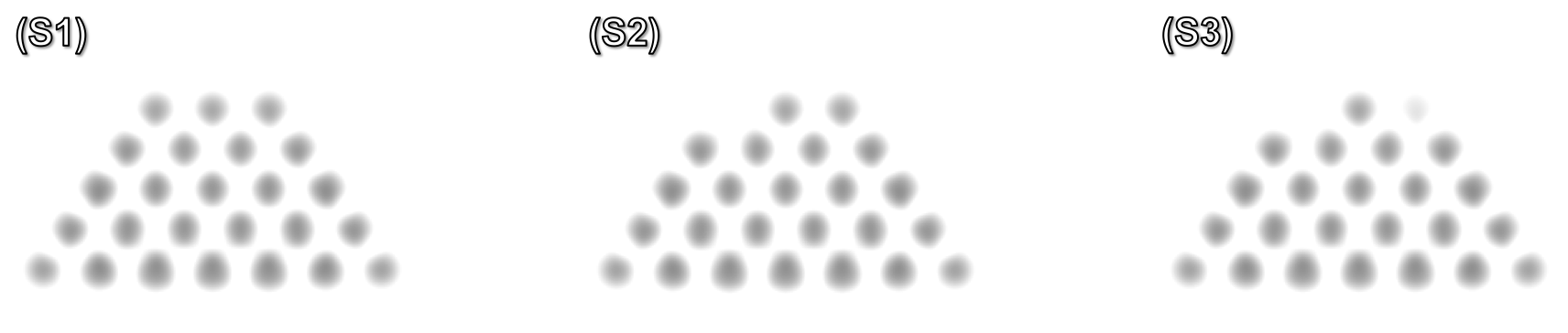
Figure 3: The three candidate configurations for generating 200-frame noisy TEM video, with dynamics.

For the static case, based on the noise-free synthetic TEM frame as Section 6, we apply 10 different Poisson noise realizations to generate the image sequence and compare the performance of our proposed algorithm with other benchmarks on both accuracy and consistency. Especially, the error boxes shown in Figure 4 indicates that our RD algorithm has the outperforming errors in most aspects if not all.

Figure 4: The error analysis under the static setting. The comparisons are conducted on the two spatial axes as well as the Euclidean errors, between RD and benchmarks including GPF (Levin, Lawrence and Crozier, 2020), AM (Nord et al., 2017), BD (Manzorro et al., 2022) and TDA (Thomas et al., 2022).

We then proceed to the dynamic case and construct the TEM video of nanoparticles with the three structural configurations in Figure 3. The series of the underlying configurations is obtained by simulating a Markov process, with a manually specified transition probability matrix

$$\blockarray{cccc}&\mbox{To S1}\mbox{To S2}\mbox{To S3}\\ \block{c(ccc)}\mbox{From S1}0.850.100.05\\ \mbox{From S2}0.300.550.15\\ \mbox{From S3}0.250.300.45\\ .$$

The surface atomic columns indexed as 23 and 25 may experience either absences or intensity changes during the video. We fix a simulated realization of the underlying configuration series and implement the algorithm on both noise-free and noisy images. The Euclidean distances between the recovered ridge points $\check{\gamma}(\tau)$ ($\tau\in[T]$) from the two sets of outputs are analyzed. With the discrete pixel resolutions of images, the results shown in Figure 5 are satisfactory, especially given that the errors for the most volatile column 23 are almost always below unit-pixel.

Figure 5: The algorithm performance under the dynamic setting. The three different underlying configurations (Figure 3) are coded by the background gray-scale levels. The fitted Euclidean deviation of selective atomic columns, from both interior (column 16) and surface (columns 23, 24, 25), are plotted for complete comparisons.

7 Conclusion

In this work, we proposed the non-parametric approach to continuously recover the ridge pattern from (TEM) videos, provided the ridge is parameterized temporally. Our algorithm explored the geometric local properties as well as the continuity restraint, and established the scores for pixels being on the ridge. The kernel-based functional estimator is used to output the ridge curve. We tailored the algorithm specially for the TEM application to tackle the disappearing and re-appearing atomic columns. We also included analysis for uncertainty quantification. Finally we evaluated our algorithm with carefully designed simulations, and implemented it on the synthetic image examples for TEM applications.

In addition to the synthetic material science applications, the algorithm may accomplish its most promising value when implemented on some real raw TEM images. Currently, the approach still has limited generalizability as it only recovers the ridge (or valley) curves with some edge degeneration scenarios. Other future directions include extending the applicability to detect connector curves, i.e., the intermediate segments between ridges and valleys (Damon, 1999). Under the time series analysis or the signal processing framework, the extension to connector curves can be useful to extract information propagation patterns, especially in topics such as impulse response analysis and change point detection.

Appendix A Gradient-yielded Alternative Approximations

Here we introduce an alternative analysis using gradient-yielded approximations as an optional supplementary update to the intermediate steps of the approach developed in the main paper. Some additional definitions and relative corollaries are summarized. Their successive remarks elaborate more details about the strengths of such gradient-yielded approximations qualitatively.

To give an overview, the introduction of the gradient-yielded quantities from Corollary 1 serves as the primary delivery of this section. These quantities have especially strong estimation power at the pixels that are within a neighborhood of non-degenerated ridge segments. Specifically, we will call those pixels as non-degenerated neighbor pixels in the following context for conciseness.

We start with the following definition introducing the normalized gradient vectors.

Definition 10.

Define the normalization of the gradient vectors $\widetilde{\nabla}(p)$ as

$$\widehat{\nabla}(p)=\widetilde{\Delta}^{+}(p)\widetilde{\nabla}(p).$$ (19)

Remark 12.

1. The normalization is motivated by the Newton’s method from optimization (Nocedal and Wright, 2006). It can help robustify the estimated gradient directions at non-degenerated neighbor pixels; see Remarks 13 and 14 for more detailed arguments.

2. For any $p$ among the non-degenerated neighbor pixels, the (estimated) Hessian matrix is usually invertible. Furthermore, the Condition 1 of Definition 1 also guarantees that $\widehat{\nabla}(p)$ as the approximation of $\Delta^{+}(p)\nabla(p)$ is nearly parallel to $v_{1}(p)$.

Given the normalized gradient estimators by Definition 10, we can obtain the following corollary that introduces approximations to the quantities proposed in Proposition 1 at those non-degenerated neighbor pixels. The proof can be found in Appendix B.

Corollary 1.

If a non-degenerated segment of the ridge $\gamma$ passes near a lattice point $p\in\Omega$, then

1. With $\widehat{\nabla}(p)$ redirected such that $\big{<}\widehat{\nabla}(p),e_{t}\big{>}\geq 0$,

   $$\hat{v}(p)=\frac{\widehat{\nabla}(p)}{\|\widehat{\nabla}(p)\|}\approx v(p).$$ (20)

2. $$\hat{\lambda}(p)=\operatorname*{argmin}_{\ell\in\mathbb{R}}\|\widetilde{\Delta}(p)\hat{v}(p)-\ell\hat{v}(p)\|=\hat{v}^{\prime}(p)\widetilde{\Delta}(p)\hat{v}(p)\approx\lambda(p).$$ (21)

3. $$\hat{\rho}(p)=\big{|}\cos\big{(}\hat{v}(p),e_{t}\big{)}\big{|}\approx\rho(p).$$ (22)

4. $$\hat{\theta}(p)=\Big{|}\cos\big{(}\hat{v}(p),\widetilde{\nabla}(p)\big{)}\Big{|}\approx\theta(p).$$ (23)

5. $$\begin{dcases}\hat{\eta}(p)=\frac{2\hat{\xi}_{2}(p)}{\hat{\xi}_{1}^{2}(p)-2\hat{\xi}_{2}(p)}\approx\eta(p)\\ \hat{\kappa}(p)=\hat{\xi}_{2}(p)-\hat{\lambda}^{2}(p)\approx\kappa(p)\end{dcases}$$ (24)

   where

   $$\hat{\xi}_{1}(p) =\operatorname{tr}\big{[}\widetilde{\Delta}(p)\big{]}-\hat{\lambda}(p)\approx\lambda_{2}(p)+\lambda_{3}(p),$$

   $$\hat{\xi}_{2}(p) =\frac{1}{2}\Big{[}\hat{\xi}^{2}_{1}(p)-\big{(}\|\widetilde{\Delta}(p)\|_{F}^{2}-\hat{\lambda}^{2}(p)\big{)}\Big{]}\approx\lambda_{2}(p)\lambda_{3}(p).$$

Remark 13.

The hatted notations in Corollary 1, e.g., $\hat{v}(p)$ and $\hat{\lambda}(p)$, always represent the gradient-yielded approximations of the eigen-related terms. For conciseness, we may not include similar corollaries for every propositions or definitions in the main paper, but the gradient-yielded counterparts for those statements can be straightforwardly derived and the notations of relative terms analogously inherit the upper hats. The two versions of quantities possess distinct features and emphasize different perspectives in practice:

1. The unhatted quantities, or those originally given in Proposition 1, manipulate the empirical eigen-decomposition of the scaled Hessian estimators (3) and aim for universal applicability. They are especially effective under degenerated scenarios. Nevertheless, they are usually accompanied with moderate performance around the non-degenerated ridge segments.

2. The gradient-yielded approximations for the eigen-terms, as proposed in Corollary 1, augment the concentration of the curve’s local directions. Specifically, these approximations will introduce a stronger force that navigates the pixels around non-degenerated ridge segments towards the true curve within a certain neighborhood. Analogous to Remark 12 and the arguments for developing the Newton’s method in optimization, it is due to the underlying landscape structure of the mapping.

We can then define the gradient-yielded intra-frame metrics analogous to Definition 5 with hatted approximations from Corollary 1, and propose the following corollary as an enhanced update of Definition 6.

Corollary 2.

Given a frame $\Omega(\tau)$ for $\tau\in[T]$, the gradient-yielded counterparts of the metrics in Definition 5 give the approximated weight for $p\in\Omega(\tau)$

$$\hat{\Phi}(p)=\exp\big{(}\hat{L}_{\rho}(p)+\hat{L}_{\theta}(p)+\hat{L}_{\eta,\kappa}(p)\big{)}.$$

And consequently update the weight and local direction by

$$v(p) \mapsto\frac{\Phi(p)v(p)+\hat{\Phi}(p)\hat{v}(p)}{\Phi(p)+\hat{\Phi}(p)}.$$ (25)

$$\Phi(p) \mapsto\Phi(p)+\hat{\Phi}(p),$$ (26)

Remark 14.

1. The Corollary 2 merges the (hatted) gradient-yielded metric designs with the (unhatted) Definition 6, and combines the featured strength of the two systems listed in Remark 13 for the enhanced estimation. In particular, the (unhatted) terms $v(p)$ and $\Phi(p)$ will supposedly dominate in (25) and (26) under degeneration scenarios, while the hatted ones will play more essential roles when considering the non-degenerated neighbor pixels.

2. The update (25) partially inherits the strengths of the gradient-yielded approximation $\hat{v}(p)$ as mentioned in Remark 13, especially at the non-degenerated neighbor pixels. In particular, the updated vector is likely to point towards the ridge curve due to the mapping’s gradient landscape.

3. If applicable, the update (25) of $v(p)$ impacts the candidate ridge tangent $v_{\gamma}(p)$ (9), which is used in the roughness penalization (Definition 7) and the curve connection (Definition 9). Similarly, the update (26) of $\Phi(p)$ affects the inter-frame weight (Definition 8), the curve connection (Definition 9) and the uncertainty statements in Section 4.

Appendix B Proof

Herein, we show detailed justification for some selected statements that appear throughout this paper.

Proof of Proposition 1 & Corollary 1.

For this proof we always consider the limiting condition that the noise level is approaching zero and the convolution effect of derivative calculation tends to vanish. For simplicity, we only show the ordinary convergence results. The extension to stochastic convergence is straightforward.

First of all, if a grid point $p$ is exactly on the ridge, the derivation of the proof is trivial from Definition 1.

Instead, suppose the grid point $p\in\Omega$ is relatively close to a ridge point $q\in\gamma$, and we will prove that the approximations are of high quality. In addition, here the eigen-related quantities for point $q$, i.e. $\{\lambda_{1}(q),\lambda_{2}(q),\lambda_{3}(q),v_{1}(q),v_{2}(q),v_{3}(q)\}$, always refer to those analytically decomposed from the exact Hessian $\Delta(q)$. Since eigen-decomposition on the Hessian matrix of a differentiable mapping is also continuous, the estimations’ approximation quality of the unhatted terms can be directly guaranteed using continuity arguments. Hence we will mainly focus on the behaviors of the gradient-yielded (hatted) quantities in Corollary 1 where $\Delta(q)$ and $\nabla(q)$ are both non-singular.

Without loss of generality, we can assume that the unit length vector $\hat{v}(p)=\frac{\widehat{\nabla}(p)}{\|\widehat{\nabla}(p)\|}$ can be expressed as the linear combination

$$\hat{v}(p)=\sum_{i=1}^{3}k_{i}v_{i}(p),\qquad\mbox{where}\qquad\sum_{i=1}^{3}k_{i}^{2}=1.$$

Note that $\widehat{\nabla}(p)=\widetilde{\Delta}^{+}(p)\widetilde{\nabla}(p)$ well approximates $\Delta^{+}(q)\nabla(q)~{}\propto~{}v_{1}(q)$ given that $q\in\gamma$ and $p$ is close to $q$.

1. Since $\hat{v}(p)=\frac{\widehat{\nabla}(p)}{\|\widehat{\nabla}(p)\|}$ is continuous with respect to non-singular $\widehat{\nabla}(p)$, and given that $\widehat{\nabla}(p)\approx\|\Delta^{+}(q)\nabla(q)\|\cdot v_{1}(q)$, then continuity implies that $\hat{v}(p)\approx v_{1}(q)$.

2. The statements on $\hat{\rho}(p)$ can be concluded directly by definition of cosine similarities.

3. From the conclusions above, we have that $k_{1}=\big{<}\hat{v}(p),v_{1}(p)\big{>}\approx\big{<}v_{1}(q),v_{1}(p)\big{>}\approx 1$, $k_{2}\approx 0$ and $k_{3}\approx 0$. Since $\hat{\lambda}(p)=\sum_{i=1}^{3}k_{i}^{2}\lambda_{i}(p)$ is continuous with respect to $k_{i}$, and $\lambda_{1}(p)\approx\lambda_{1}(q)$, we conclude that $\hat{\lambda}(p)\approx\lambda_{1}(q)$.

4. It directly follows from the first point above given continuity.

5. It suffices to show that $\hat{\xi}_{1}(p)\approx\lambda_{2}(q)+\lambda_{3}(q)$ and $\hat{\xi}_{2}(p)\approx\lambda_{2}(q)\lambda_{3}(q)$. Some calculations give

   $$\hat{\xi}_{1}(p)=\sum_{i=1}^{3}(1-k_{i})\lambda_{i}(p),\qquad\hat{\xi}_{2}(p)=\lambda_{2}(p)\lambda_{3}(p)+\big{(}\lambda_{1}(p)-\hat{\lambda}(p)\big{)}\big{(}\lambda_{2}(p)+\lambda_{3}(p)-\hat{\lambda}(p)\big{)}.$$

   Then the convergence statements follow by continuity again.

Under degeneration, on the other hand, the gradient-yielded approximations can perform rather poorly, but they still give bounded quantities and will be compensated by the original unhatted terms in Corollary 2 based on our algorithm designs. ∎

Proof of Proposition 2.

1. The monotonicity statement is true according to the definition of cosine similarity. Since $\max L_{\rho}(p)=2$, then $L_{\rho}(p)=2\Leftrightarrow\rho(p)=1\Leftrightarrow v(p)$ is parallel to the temporal indicator $e_{t}$.

2. The monotonicity statement is true according to the definition of cosine similarity. Since $\max L_{\theta}(p)=2$, then $L_{\theta}(p)=2\Leftrightarrow\theta(p)=1\Leftrightarrow v(p)$ is parallel to $\widetilde{\Delta}(p)\widehat{\nabla}(p)=\widetilde{\nabla}(p)$.

3. It can be shown with simple algebra that

   $$\frac{2}{\eta(p)}=\frac{\lambda_{2}(p)}{\lambda_{3}(p)}+\frac{\lambda_{3}(p)}{\lambda_{2}(p)}\in(-\infty,-2]~{}\bigcup~{}[2,\infty).$$

   It implies that $\eta(p)$ is positive only when $\lambda_{2}(p)$ and $\lambda_{3}(p)$ have the same sign, and the maximum $\eta(p)=1$ is attained if and only if $\lambda_{2}(p)/\lambda_{3}(p)=1$. In addition, since $L_{\eta,\kappa}(p)$ is monotonic with respect to both $\eta(p)$ and the product $\lambda_{2}(p)\lambda_{3}(p)$ due to monotonicity-conserved composition with $\kappa(p)$, respectively, the sub-statement holds.

Similar derivations for the gradient-yielded version can be analogously obtained. ∎

[Acknowledgments] The authors thank Ramon Manzorro (University of Cádiz) and Professor Peter A. Crozier’s lab members for assistance in imaging simulations, data handling and material science background education. The authors gratefully acknowledge financial support from National Science Foundation Awards 2114143, 1934985, 1940124, and 1940276.

References

- Alhasson et al. (2021) {barticle}[author] \bauthor\bsnmAlhasson, \bfnmHaifa F.\binitsH. F., \bauthor\bsnmWillcocks, \bfnmChris G.\binitsC. G., \bauthor\bsnmAlharbi, \bfnmShuaa S.\binitsS. S., \bauthor\bsnmKasim, \bfnmAdetayo\binitsA. and \bauthor\bsnmObara, \bfnmBoguslaw\binitsB. (\byear2021). \btitleThe Relationship between Curvilinear Structure Enhancement and Ridge Detection Methods. \bjournalThe Visual Computer \bvolume37 \bpages2263–2283. \bdoi10.1007/s00371-020-01985-4 \endbibitem
- Ameli, Desai and Shadden (2014) {binproceedings}[author] \bauthor\bsnmAmeli, \bfnmSiavash\binitsS., \bauthor\bsnmDesai, \bfnmYogin\binitsY. and \bauthor\bsnmShadden, \bfnmShawn C.\binitsS. C. (\byear2014). \btitleDevelopment of an Efficient and Flexible Pipeline for Lagrangian Coherent Structure Computation. In \bbooktitleTopological Methods in Data Analysis and Visualization III (\beditor\bfnmPeer-Timo\binitsP.-T. \bsnmBremer, \beditor\bfnmIngrid\binitsI. \bsnmHotz, \beditor\bfnmValerio\binitsV. \bsnmPascucci and \beditor\bfnmRonald\binitsR. \bsnmPeikert, eds.). \bseriesMathematics and Visualization \bpages201–215. \bpublisherSpringer International Publishing, \baddressCham. \bdoi10.1007/978-3-319-04099-8_13 \endbibitem
- Beyeler, Mirus and Verl (2014) {binproceedings}[author] \bauthor\bsnmBeyeler, \bfnmMichael\binitsM., \bauthor\bsnmMirus, \bfnmFlorian\binitsF. and \bauthor\bsnmVerl, \bfnmAlexander\binitsA. (\byear2014). \btitleVision-Based Robust Road Lane Detection in Urban Environments. In \bbooktitle2014 IEEE International Conference on Robotics and Automation (ICRA) \bpages4920–4925. \bdoi10.1109/ICRA.2014.6907580 \endbibitem
- Cheng, Hall and Turlach (1999) {barticle}[author] \bauthor\bsnmCheng, \bfnmMing-Yen\binitsM.-Y., \bauthor\bsnmHall, \bfnmPeter\binitsP. and \bauthor\bsnmTurlach, \bfnmBerwin A.\binitsB. A. (\byear1999). \btitleHigh-Derivative Parametric Enhancements of Nonparametric Curve Estimators. \bjournalBiometrika \bvolume86 \bpages417–428. \endbibitem
- Colominas, Meignen and Pham (2020) {barticle}[author] \bauthor\bsnmColominas, \bfnmMarcelo A.\binitsM. A., \bauthor\bsnmMeignen, \bfnmSylvain\binitsS. and \bauthor\bsnmPham, \bfnmDuong-Hung\binitsD.-H. (\byear2020). \btitleFully Adaptive Ridge Detection Based on STFT Phase Information. \bjournalIEEE Signal Processing Letters \bvolume27 \bpages620–624. \bdoi10.1109/LSP.2020.2987166 \endbibitem
- Damon (1999) {barticle}[author] \bauthor\bsnmDamon, \bfnmJames\binitsJ. (\byear1999). \btitleProperties of Ridges and Cores for Two-Dimensional Images. \bjournalJournal of Mathematical Imaging and Vision \bvolume10 \bpages163–174. \bdoi10.1023/A:1008379107611 \endbibitem
- Egerton (2013) {barticle}[author] \bauthor\bsnmEgerton, \bfnmR. F.\binitsR. F. (\byear2013). \btitleControl of Radiation Damage in the TEM. \bjournalUltramicroscopy \bvolume127 \bpages100–108. \bdoi10.1016/j.ultramic.2012.07.006 \endbibitem
- Egerton (2019) {barticle}[author] \bauthor\bsnmEgerton, \bfnmR. F.\binitsR. F. (\byear2019). \btitleRadiation Damage to Organic and Inorganic Specimens in the TEM. \bjournalMicron \bvolume119 \bpages72–87. \bdoi10.1016/j.micron.2019.01.005 \endbibitem
- Egerton, Li and Malac (2004) {barticle}[author] \bauthor\bsnmEgerton, \bfnmR. F.\binitsR. F., \bauthor\bsnmLi, \bfnmP.\binitsP. and \bauthor\bsnmMalac, \bfnmM.\binitsM. (\byear2004). \btitleRadiation Damage in the TEM and SEM. \bjournalMicron \bvolume35 \bpages399–409. \bdoi10.1016/j.micron.2004.02.003 \endbibitem
- Fan and Yao (2008) {bbook}[author] \bauthor\bsnmFan, \bfnmJianqing\binitsJ. and \bauthor\bsnmYao, \bfnmQiwei\binitsQ. (\byear2008). \btitleNonlinear Time Series: Nonparametric and Parametric Methods. \bpublisherSpringer Science & Business Media. \endbibitem
- Faruqi and McMullan (2018) {barticle}[author] \bauthor\bsnmFaruqi, \bfnmA. R.\binitsA. R. and \bauthor\bsnmMcMullan, \bfnmG.\binitsG. (\byear2018). \btitleDirect Imaging Detectors for Electron Microscopy. \bjournalNuclear Instruments and Methods in Physics Research Section A: Accelerators, Spectrometers, Detectors and Associated Equipment \bvolume878 \bpages180–190. \bdoi10.1016/j.nima.2017.07.037 \endbibitem
- Frangi et al. (1998) {bincollection}[author] \bauthor\bsnmFrangi, \bfnmAlejandro F.\binitsA. F., \bauthor\bsnmNiessen, \bfnmWiro J.\binitsW. J., \bauthor\bsnmVincken, \bfnmKoen L.\binitsK. L. and \bauthor\bsnmViergever, \bfnmMax A.\binitsM. A. (\byear1998). \btitleMultiscale Vessel Enhancement Filtering. In \bbooktitleMedical Image Computing and Computer-Assisted Intervention — MICCAI’98, (\beditor\bfnmWilliam M.\binitsW. M. \bsnmWells, \beditor\bfnmAlan\binitsA. \bsnmColchester and \beditor\bfnmScott\binitsS. \bsnmDelp, eds.) \bvolume1496 \bpages130–137. \bpublisherSpringer Berlin Heidelberg, \baddressBerlin, Heidelberg. \bdoi10.1007/BFb0056195 \endbibitem
- Green and Silverman (1994) {bbook}[author] \bauthor\bsnmGreen, \bfnmP. J.\binitsP. J. and \bauthor\bsnmSilverman, \bfnmB. W.\binitsB. W. (\byear1994). \btitleNonparametric Regression and Generalized Linear Models: A Roughness Penalty Approach, \bedition1st ed ed. \bseriesMonographs on Statistics and Applied Probability (Series). \bpublisherChapman & Hall, \baddressLondon. \endbibitem
- Haller (2002) {barticle}[author] \bauthor\bsnmHaller, \bfnmG.\binitsG. (\byear2002). \btitleLagrangian Coherent Structures from Approximate Velocity Data. \bjournalPhysics of Fluids \bvolume14 \bpages1851–1861. \bdoi10.1063/1.1477449 \endbibitem
- Haller and Yuan (2000) {barticle}[author] \bauthor\bsnmHaller, \bfnmG.\binitsG. and \bauthor\bsnmYuan, \bfnmG.\binitsG. (\byear2000). \btitleLagrangian Coherent Structures and Mixing in Two-Dimensional Turbulence. \bjournalPhysica D: Nonlinear Phenomena \bvolume147 \bpages352–370. \bdoi10.1016/S0167-2789(00)00142-1 \endbibitem
- Kasten et al. (2009) {binproceedings}[author] \bauthor\bsnmKasten, \bfnmJens\binitsJ., \bauthor\bsnmPetz, \bfnmChristoph\binitsC., \bauthor\bsnmHotz, \bfnmIngrid\binitsI., \bauthor\bsnmNoack, \bfnmBernd R.\binitsB. R. and \bauthor\bsnmHege, \bfnmHans-Christian\binitsH.-C. (\byear2009). \btitleLocalized Finite-Time Lyapunov Exponent for Unsteady Flow Analysis. In \bbooktitleVision Modeling and Visualization \bpages265–276. \endbibitem
- Laurent and Meignen (2022) {barticle}[author] \bauthor\bsnmLaurent, \bfnmNils\binitsN. and \bauthor\bsnmMeignen, \bfnmSylvain\binitsS. (\byear2022). \btitleA Novel Ridge Detector for Nonstationary Multicomponent Signals: Development and Application to Robust Mode Retrieval. \bjournalarXiv preprint arXiv:2009.13123. \bdoi10.48550/arXiv.2009.13123 \endbibitem
- Lawrence et al. (2020) {barticle}[author] \bauthor\bsnmLawrence, \bfnmEthan L.\binitsE. L., \bauthor\bsnmLevin, \bfnmBarnaby D. A.\binitsB. D. A., \bauthor\bsnmMiller, \bfnmBenjamin K.\binitsB. K. and \bauthor\bsnmCrozier, \bfnmPeter A.\binitsP. A. (\byear2020). \btitleApproaches to Exploring Spatio-Temporal Surface Dynamics in Nanoparticles with In Situ Transmission Electron Microscopy. \bjournalMicroscopy and Microanalysis \bvolume26 \bpages86–94. \bdoi10.1017/S1431927619015228 \endbibitem
- Lawrence et al. (2021) {barticle}[author] \bauthor\bsnmLawrence, \bfnmEthan L.\binitsE. L., \bauthor\bsnmLevin, \bfnmBarnaby D. A.\binitsB. D. A., \bauthor\bsnmBoland, \bfnmTara\binitsT., \bauthor\bsnmChang, \bfnmShery L. Y.\binitsS. L. Y. and \bauthor\bsnmCrozier, \bfnmPeter A.\binitsP. A. (\byear2021). \btitleAtomic Scale Characterization of Fluxional Cation Behavior on Nanoparticle Surfaces: Probing Oxygen Vacancy Creation/Annihilation at Surface Sites. \bjournalACS Nano \bvolume15 \bpages2624–2634. \bdoi10.1021/acsnano.0c07584 \endbibitem
- Levin (2021) {barticle}[author] \bauthor\bsnmLevin, \bfnmBarnaby D. A.\binitsB. D. A. (\byear2021). \btitleDirect Detectors and Their Applications in Electron Microscopy for Materials Science. \bjournalJournal of Physics: Materials \bvolume4 \bpages042005. \bdoi10.1088/2515-7639/ac0ff9 \endbibitem
- Levin, Lawrence and Crozier (2020) {barticle}[author] \bauthor\bsnmLevin, \bfnmBarnaby D. A.\binitsB. D. A., \bauthor\bsnmLawrence, \bfnmEthan L.\binitsE. L. and \bauthor\bsnmCrozier, \bfnmPeter A.\binitsP. A. (\byear2020). \btitleTracking the Picoscale Spatial Motion of Atomic Columns during Dynamic Structural Change. \bjournalUltramicroscopy \bvolume213 \bpages112978. \bdoi10.1016/j.ultramic.2020.112978 \endbibitem
- Lin et al. (2021) {barticle}[author] \bauthor\bsnmLin, \bfnmRuoqian\binitsR., \bauthor\bsnmZhang, \bfnmRui\binitsR., \bauthor\bsnmWang, \bfnmChunyang\binitsC., \bauthor\bsnmYang, \bfnmXiao-Qing\binitsX.-Q. and \bauthor\bsnmXin, \bfnmHuolin L.\binitsH. L. (\byear2021). \btitleTEMImageNet Training Library and AtomSegNet Deep-Learning Models for High-Precision Atom Segmentation, Localization, Denoising, and Deblurring of Atomic-Resolution Images. \bjournalScientific Reports \bvolume11 \bpages5386. \bdoi10.1038/s41598-021-84499-w \endbibitem
- Lindeberg (1996) {binproceedings}[author] \bauthor\bsnmLindeberg, \bfnmT.\binitsT. (\byear1996). \btitleEdge Detection and Ridge Detection with Automatic Scale Selection. In \bbooktitleProceedings CVPR IEEE Computer Society Conference on Computer Vision and Pattern Recognition \bpages465–470. \bdoi10.1109/CVPR.1996.517113 \endbibitem
- Lindeberg (1998) {barticle}[author] \bauthor\bsnmLindeberg, \bfnmTony\binitsT. (\byear1998). \btitleFeature Detection with Automatic Scale Selection. \bjournalInternational Journal of Computer Vision \bvolume30 \bpages79–116. \bdoi10.1023/A:1008045108935 \endbibitem
- Lindeberg and Almansa (2000) {barticle}[author] \bauthor\bsnmLindeberg, \bfnmT.\binitsT. and \bauthor\bsnmAlmansa, \bfnmA.\binitsA. (\byear2000). \btitleFingerprint Enhancement by Shape Adaptation of Scale-Space Operators with Automatic Scale Selection. \bjournalIEEE Transactions on Image Processing \bvolume9 \bpages2027–2042. \bdoi10.1109/83.887971 \endbibitem
- Lopez et al. (1999) {barticle}[author] \bauthor\bsnmLopez, \bfnmA. M.\binitsA. M., \bauthor\bsnmLumbreras, \bfnmF.\binitsF., \bauthor\bsnmSerrat, \bfnmJ.\binitsJ. and \bauthor\bsnmVillanueva, \bfnmJ. J.\binitsJ. J. (\byear1999). \btitleEvaluation of Methods for Ridge and Valley Detection. \bjournalIEEE Transactions on Pattern Analysis and Machine Intelligence \bvolume21 \bpages327–335. \bdoi10.1109/34.761263 \endbibitem
- Lopez-Molina et al. (2015) {barticle}[author] \bauthor\bsnmLopez-Molina, \bfnmC.\binitsC., \bauthor\bsnmVidal-Diez de Ulzurrun, \bfnmG.\binitsG., \bauthor\bsnmBaetens, \bfnmJ. M.\binitsJ. M., \bauthor\bsnmVan den Bulcke, \bfnmJ.\binitsJ. and \bauthor\bsnmDe Baets, \bfnmB.\binitsB. (\byear2015). \btitleUnsupervised Ridge Detection Using Second Order Anisotropic Gaussian Kernels. \bjournalSignal Processing \bvolume116 \bpages55–67. \bdoi10.1016/j.sigpro.2015.03.024 \endbibitem
- Manzorro et al. (2022) {barticle}[author] \bauthor\bsnmManzorro, \bfnmRamon\binitsR., \bauthor\bsnmXu, \bfnmYuchen\binitsY., \bauthor\bsnmVincent, \bfnmJoshua L.\binitsJ. L., \bauthor\bsnmRivera, \bfnmRoberto\binitsR., \bauthor\bsnmMatteson, \bfnmDavid S.\binitsD. S. and \bauthor\bsnmCrozier, \bfnmPeter A.\binitsP. A. (\byear2022). \btitleExploring Blob Detection to Determine Atomic Column Positions and Intensities in Time-Resolved TEM Images with Ultra-Low Signal-to-Noise. \bjournalMicroscopy and Microanalysis \bpages1–14. \bdoi10.1017/S1431927622000356 \endbibitem
- Mathur et al. (2007) {barticle}[author] \bauthor\bsnmMathur, \bfnmManikandan\binitsM., \bauthor\bsnmHaller, \bfnmGeorge\binitsG., \bauthor\bsnmPeacock, \bfnmThomas\binitsT., \bauthor\bsnmRuppert-Felsot, \bfnmJori E.\binitsJ. E. and \bauthor\bsnmSwinney, \bfnmHarry L.\binitsH. L. (\byear2007). \btitleUncovering the Lagrangian Skeleton of Turbulence. \bjournalPhysical Review Letters \bvolume98 \bpages144502. \bdoi10.1103/PhysRevLett.98.144502 \endbibitem
- Meijering et al. (2004) {barticle}[author] \bauthor\bsnmMeijering, \bfnmE.\binitsE., \bauthor\bsnmJacob, \bfnmM.\binitsM., \bauthor\bsnmSarria, \bfnmJ. C. F.\binitsJ. C. F., \bauthor\bsnmSteiner, \bfnmP.\binitsP., \bauthor\bsnmHirling, \bfnmH.\binitsH. and \bauthor\bsnmUnser, \bfnmM.\binitsM. (\byear2004). \btitleDesign and Validation of a Tool for Neurite Tracing and Analysis in Fluorescence Microscopy Images. \bjournalCytometry \bvolume58A \bpages167–176. \bdoi10.1002/cyto.a.20022 \endbibitem
- Ng et al. (2015) {bincollection}[author] \bauthor\bsnmNg, \bfnmChoon-Ching\binitsC.-C., \bauthor\bsnmYap, \bfnmMoi Hoon\binitsM. H., \bauthor\bsnmCosten, \bfnmNicholas\binitsN. and \bauthor\bsnmLi, \bfnmBaihua\binitsB. (\byear2015). \btitleAutomatic Wrinkle Detection Using Hybrid Hessian Filter. In \bbooktitleComputer Vision – ACCV 2014, (\beditor\bfnmDaniel\binitsD. \bsnmCremers, \beditor\bfnmIan\binitsI. \bsnmReid, \beditor\bfnmHideo\binitsH. \bsnmSaito and \beditor\bfnmMing-Hsuan\binitsM.-H. \bsnmYang, eds.) \bvolume9005 \bpages609–622. \bpublisherSpringer International Publishing, \baddressCham. \bdoi10.1007/978-3-319-16811-1_40 \endbibitem
- Nocedal and Wright (2006) {bbook}[author] \bauthor\bsnmNocedal, \bfnmJorge\binitsJ. and \bauthor\bsnmWright, \bfnmStephen\binitsS. (\byear2006). \btitleNumerical Optimization. \bpublisherSpringer Science & Business Media. \endbibitem
- Nord et al. (2017) {barticle}[author] \bauthor\bsnmNord, \bfnmMagnus\binitsM., \bauthor\bsnmVullum, \bfnmPer Erik\binitsP. E., \bauthor\bsnmMacLaren, \bfnmIan\binitsI., \bauthor\bsnmTybell, \bfnmThomas\binitsT. and \bauthor\bsnmHolmestad, \bfnmRandi\binitsR. (\byear2017). \btitleAtomap: A New Software Tool for the Automated Analysis of Atomic Resolution Images Using Two-Dimensional Gaussian Fitting. \bjournalAdvanced Structural and Chemical Imaging \bvolume3 \bpages9. \bdoi10.1186/s40679-017-0042-5 \endbibitem
- Norgard and Bremer (2013) {barticle}[author] \bauthor\bsnmNorgard, \bfnmGregory\binitsG. and \bauthor\bsnmBremer, \bfnmPeer-Timo\binitsP.-T. (\byear2013). \btitleRidge–Valley Graphs: Combinatorial Ridge Detection Using Jacobi Sets. \bjournalComputer Aided Geometric Design \bvolume30 \bpages597–608. \bdoi10.1016/j.cagd.2012.03.015 \endbibitem
- Pham et al. (2021) {barticle}[author] \bauthor\bsnmPham, \bfnmLuan Thanh\binitsL. T., \bauthor\bsnmOksum, \bfnmErdinc\binitsE., \bauthor\bsnmVu, \bfnmMinh Duc\binitsM. D., \bauthor\bsnmVo, \bfnmQuynh Thanh\binitsQ. T., \bauthor\bsnmDu Le-Viet, \bfnmKhuong\binitsK. and \bauthor\bsnmEldosouky, \bfnmAhmed M.\binitsA. M. (\byear2021). \btitleAn Improved Approach for Detecting Ridge Locations to Interpret the Potential Field Data for More Accurate Structural Mapping: A Case Study from Vredefort Dome Area (South Africa). \bjournalJournal of African Earth Sciences \bvolume175 \bpages104099. \bdoi10.1016/j.jafrearsci.2020.104099 \endbibitem
- Porteous (2001) {bbook}[author] \bauthor\bsnmPorteous, \bfnmI. R.\binitsI. R. (\byear2001). \btitleGeometric Differentiation: For the Intelligence of Curves and Surfaces. \bpublisherCambridge University Press. \endbibitem
- Reisenhofer and King (2019) {barticle}[author] \bauthor\bsnmReisenhofer, \bfnmRafael\binitsR. and \bauthor\bsnmKing, \bfnmEmily J.\binitsE. J. (\byear2019). \btitleEdge, Ridge, and Blob Detection with Symmetric Molecules. \bjournalSIAM Journal on Imaging Sciences \bvolume12 \bpages1585–1626. \bdoi10.1137/19M1240861 \endbibitem
- Ruskin, Yu and Grigorieff (2013) {barticle}[author] \bauthor\bsnmRuskin, \bfnmRachel S.\binitsR. S., \bauthor\bsnmYu, \bfnmZhiheng\binitsZ. and \bauthor\bsnmGrigorieff, \bfnmNikolaus\binitsN. (\byear2013). \btitleQuantitative Characterization of Electron Detectors for Transmission Electron Microscopy. \bjournalJournal of Structural Biology \bvolume184 \bpages385–393. \bdoi10.1016/j.jsb.2013.10.016 \endbibitem
- Sato et al. (1998) {barticle}[author] \bauthor\bsnmSato, \bfnmYoshinobu\binitsY., \bauthor\bsnmNakajima, \bfnmShin\binitsS., \bauthor\bsnmShiraga, \bfnmNobuyuki\binitsN., \bauthor\bsnmAtsumi, \bfnmHideki\binitsH., \bauthor\bsnmYoshida, \bfnmShigeyuki\binitsS., \bauthor\bsnmKoller, \bfnmThomas\binitsT., \bauthor\bsnmGerig, \bfnmGuido\binitsG. and \bauthor\bsnmKikinis, \bfnmRon\binitsR. (\byear1998). \btitleThree-Dimensional Multi-Scale Line Filter for Segmentation and Visualization of Curvilinear Structures in Medical Images. \bjournalMedical Image Analysis \bvolume2 \bpages143–168. \bdoi10.1016/S1361-8415(98)80009-1 \endbibitem
- Schindler et al. (2012) {bincollection}[author] \bauthor\bsnmSchindler, \bfnmBenjamin\binitsB., \bauthor\bsnmPeikert, \bfnmRonald\binitsR., \bauthor\bsnmFuchs, \bfnmRaphael\binitsR. and \bauthor\bsnmTheisel, \bfnmHolger\binitsH. (\byear2012). \btitleRidge Concepts for the Visualization of Lagrangian Coherent Structures. In \bbooktitleTopological Methods in Data Analysis and Visualization II: Theory, Algorithms, and Applications, (\beditor\bfnmRonald\binitsR. \bsnmPeikert, \beditor\bfnmHelwig\binitsH. \bsnmHauser, \beditor\bfnmHamish\binitsH. \bsnmCarr and \beditor\bfnmRaphael\binitsR. \bsnmFuchs, eds.). \bseriesMathematics and Visualization \bpages221–235. \bpublisherSpringer, \baddressBerlin, Heidelberg. \bdoi10.1007/978-3-642-23175-9_15 \endbibitem
- Senatore and Ross (2011) {barticle}[author] \bauthor\bsnmSenatore, \bfnmCarmine\binitsC. and \bauthor\bsnmRoss, \bfnmShane D.\binitsS. D. (\byear2011). \btitleDetection and Characterization of Transport Barriers in Complex Flows via Ridge Extraction of the Finite Time Lyapunov Exponent Field. \bjournalInternational Journal for Numerical Methods in Engineering \bvolume86 \bpages1163–1174. \bdoi10.1002/nme.3101 \endbibitem
- Shokouh et al. (2021) {barticle}[author] \bauthor\bsnmShokouh, \bfnmGhulam-Sakhi\binitsG.-S., \bauthor\bsnmMagnier, \bfnmBaptiste\binitsB., \bauthor\bsnmXu, \bfnmBinbin\binitsB. and \bauthor\bsnmMontesinos, \bfnmPhilippe\binitsP. (\byear2021). \btitleRidge Detection by Image Filtering Techniques: A Review and an Objective Analysis. \bjournalPattern Recognition and Image Analysis \bvolume31 \bpages551–570. \bdoi10.1134/S1054661821030226 \endbibitem
- Thomas et al. (2022) {barticle}[author] \bauthor\bsnmThomas, \bfnmAndrew M.\binitsA. M., \bauthor\bsnmCrozier, \bfnmPeter A.\binitsP. A., \bauthor\bsnmXu, \bfnmYuchen\binitsY. and \bauthor\bsnmMatteson, \bfnmDavid S.\binitsD. S. (\byear2022). \btitleDetection and Hypothesis Testing of Features in Extremely Noisy Image Series Using Topological Data Analysis, with Applications to Nanoparticle Videos. \bjournalarXiv preprint arXiv:2209.13854. \bdoi10.48550/arXiv.2209.13584 \endbibitem
- van der Walt et al. (2014) {barticle}[author] \bauthor\bsnmvan der Walt, \bfnmStéfan\binitsS., \bauthor\bsnmSchönberger, \bfnmJohannes L.\binitsJ. L., \bauthor\bsnmNunez-Iglesias, \bfnmJuan\binitsJ., \bauthor\bsnmBoulogne, \bfnmFrançois\binitsF., \bauthor\bsnmWarner, \bfnmJoshua D.\binitsJ. D., \bauthor\bsnmYager, \bfnmNeil\binitsN., \bauthor\bsnmGouillart, \bfnmEmmanuelle\binitsE. and \bauthor\bsnmYu, \bfnmTony\binitsT. (\byear2014). \btitleScikit-Image: Image Processing in Python. \bjournalPeerJ \bvolume2 \bpagese453. \bdoi10.7717/peerj.453 \endbibitem
- Vincent and Crozier (2021) {barticle}[author] \bauthor\bsnmVincent, \bfnmJoshua L.\binitsJ. L. and \bauthor\bsnmCrozier, \bfnmPeter A.\binitsP. A. (\byear2021). \btitleFluxional Behavior at the Atomic Level and Its Impact on Activity: CO Oxidation over CeO2-Supported Pt Catalysts. \bjournalarXiv preprint arXiv:2104.00821. \bdoi10.48550/arXiv.2104.00821 \endbibitem