Beyond KNN: Deep Neighborhood Learning for WiFi-based Indoor Positioning Systems

Abstract

K-Neares Neighbors (KNN) and its variant weighted KNN (WKNN) have been explored for years in both academy and industry to provide stable and reliable performance in WiFi-based indoor positioning systems. Such algorithms estimate the location of a given point based on the locality information from the selected nearest WiFi neighbors according to some distance metrics calculated from the combination of WiFi received signal strength (RSS). However, such a process does not consider the relational information among the given point, WiFi neighbors, and the WiFi access points (WAPs). Therefore, this study proposes a novel Deep Neighborhood Learning (DNL). The proposed DNL approach converts the WiFi neighborhood to heterogeneous graphs, and utilizes deep graph learning to extract better representation of the WiFi neighborhood to improve the positioning accuracy. Experiments on 3 real industrial datasets collected from 3 mega shopping malls on 26 floors have shown that the proposed approach can reduce the mean absolute positioning error by 10% to 50% in most of the cases. Specially, the proposed approach sharply reduces the root mean squared positioning error and 95% percentile positioning error, being more robust to the outliers than conventional KNN and WKNN.

I Introduction

The proliferation of smartphones has provided an excellent tool to keep people connected, provide them with the latest information, and in general making life easier for many. These devices and the applications around them provide services tailored to the user and their context, but they rely on up to date information about the device. Among the most useful information is the position of the user, that in outdoor scenarios is typically obtained using Global Navigation Satellite Systems. In indoor scenarios due to the attenuation and multipaths of the signals, the accuracy of the positioning is severely affected [1] and the service needs to rely on other technologies and techniques to improve it.

In most indoor environments, the devices are able to connect to many wireless networks that can be used for positioning including cellular, WiFi, Bluetooth, Ultra Wide Band, among others. The most widely deployed technology is WiFi, and as an example, in shopping malls it is typically possible to observe between ten and hundreds of WiFi access points (WAP) at any given point near shops. The WiFi technology offers several metrics that can be used for positioning [2], including the angle of Arrival [3, 4], time of arrival [5, 6], time difference of arrival [7] and the received signal strength (RSS) [8, 9]. Among those, the RSS has become one of the most commonly used sources of information because it does not require extra hardware and it is available in all devices. In open spaces, it is possible to implement a trilateration from the position of the WAPs, and estimating the distances to the user with the RSS measured in dB and a log distance model [10], but even if the positions were known, that model changes according to the unknown conditions of the obstructions between the user and the WAPs.

As a way to overcome the non predictable distribution of the RSS values with position, is it common to measure the RSS values from all observable WAPs in a grid of samples covering all the areas of interest. These measurements can be used to estimate more complex models of the RSS-distance models [11], the RSS-position model [12], as reference points (fingerprints) in a weighted K-Nearest Neighbors (WKNN) estimation [13, 14, 15, 16], or other machine learning methods [17, 18, 19, 20]. In most cases it has been observed that the wide distribution of the data in the RSS-distance and RSS-position modeling doesn’t allow to have a local model, but in the WKNN estimation, it only use the locality of the neighbors, but we loose the information from the RSS values. The authors of this paper propose Deep Neighborhood Learning to analyse the RSS distribution using a deep graph neural network-based model but focusing in the local community or neighborhood of similar reference points.

The contributions of this work are summarized as follows:

• We propose a novel Deep Neighborhood Learning approach to extract better representation of the WiFi neighborhood to improve the positioning accuracy.

• In the proposed approach, we develop a deep graph neural network-based positioning model to learn the relational information (the topology and the features) from the WiFi neighborhood.

• Compared to conventional positioning algorithms using the WiFi neighborhood, the experiments on three real large datasets have shown that the proposed approach can sharply reduce the positioning error and the influence from the outliers.

The rest of the paper is distributed as follows: Section II will discuss the proposed architecture, Section III will describe the experiments, Section IV will show the results and analyse them, and in Section V we will draw the general conclusions.

II Methodology

As illustrated above, to overcome the challenges of missing RSS features in conventional KNN and its variant WKNN, we propose a Deep Neighborhood Learning approach to learn the relation among one given fingerprint (FP) and its WiFi neighbors, and hence provide better positioning accuracy for WiFi-based indoor positioning systems.

II-A The local community

A local community represents a snapshot of the RSS distributions in the vicinity of any given FP. Each local community is constructed from a center/target FP (TFP) and its closest neighbor FPs (NFP), as well as all the WiFi measurements that can be detected among the FPs in the local community.

To select the NFPs of a certain TFP, we first calculate the distance from the center/target FP to all the reference FPs. In this work, we use the Manhattan distance to represent the distance between two FPs in the signal space. The Manhattan distance has been shown to be effective to represent the similarity between two WiFi fingerprints, and has been adopted by many WiFi fingerprinting-based positioning algorithms [14, 15, 16]. Supposing there are $n$ WAPs in the entire dataset, the RSS values of one FP are converted to a vector of length $n$, where the non-detected signals are padding with a default value of 0. So that the Manhattan distance between the two FP vectors of $FP_{1}=[RSS_{1}^{1},RSS_{2}^{1},...RSS_{n}^{1}]$ and $FP_{2}=[RSS_{1}^{2},RSS_{2}^{2},...RSS_{n}^{2}]$ can be calculated by:

$$|FP_{1}-FP_{2}|=\sum_{i=1}^{n}\left|RSS_{i}^{1}-RSS_{i}^{2}\right|$$ (1)

Therefore, for $m$ FPs, we will have $m$ TFPs, and accordingly $m-1$ distances from a certain TFP to all other reference FPs. We select the top $k$ FPs with the shortest distance as the NFPs. The local community will consist of the target FP and the neighbor FPs as:

$$C=\{TFP,NFP_{1},NFP_{2},...,NFP_{k}\}$$ (2)

II-B Graph representations of local communities

The local communities represent more than just the fingerprints that are similar to the TFP, the relationships established by the RSS observed by the members of that set to the WAPs in the vicinity offer a glimpse of the local model of RSS in there. The community can be represented as a heterogeneous graph as described in [21], but focusing only in the area of interest. Given a training reference set and a test set, 2 types of graphs constructions are required, the neighbors graphs in the training reference set, where each reference FP finds neighbors in the rest of the training set, and the neighbors graphs in the test set, where each test FP finds the neighbors among the training set. In the training case, the graph shown in Figure 1 can be created with 3 types of nodes, the neighbor FPs, the target FP and the WAP nodes. The neighbor FP nodes include information about the position of that reference point ($F_{W}$), the target FP has a position masked with zeros, and the WAP node stores the MAC index of the WAP ($F_{A}$). The observations of each FP ($FP_{i}=\{MAC_{i_{1}}:RSS_{i_{1}},...,MAC_{i_{n}}:RSS_{i_{n}}\}$) are encoded in the edges between FP nodes and WAP nodes ($E_{W\rightarrow A}$ and $E_{A\rightarrow W}$), where the edge from (to) WAP node $i$ to (from) FP node $j$ has a weight equal to the RSS observed in FP $j$ for WAP $i$. Each graph of the local community of TFP $i$ in the dataset for training can be denoted by $g_{train}(i)=\{F_{W},F_{A},E_{W\rightarrow A},E_{A\rightarrow W}\}$. Each graph is associated with a label of the location of the TFP node.

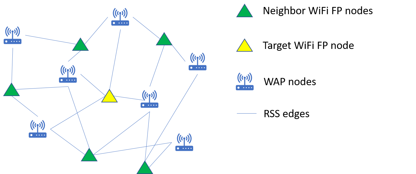
Figure 1: An example of the graph representation of the local community for training.

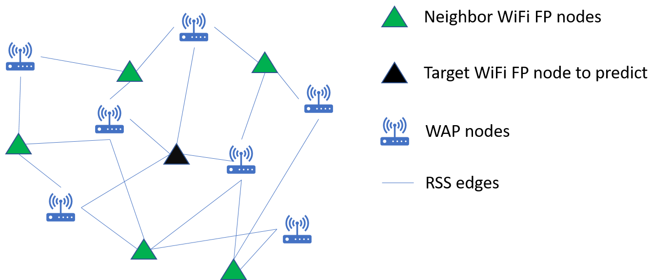
Figure 2: An example of the graph representation of the local community for inference/testing.

For inference of the test set, the TFP $j$ has no label, but the same method to construct a local community is used, selecting the NFPs from the training dataset, and constructing a similar graph $g_{inf}(j)$ as shown in Figure 2.

II-C Positioning with Deep Neighborhood Learning

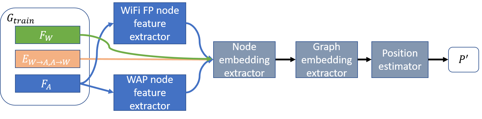
Figure 3: Structure of the proposed supervised deep graph neural networks-based positioning model.

The positioning problem is now translated to making inference of the unlabeled graph $g_{inf}$ by a model trained with labeled graphs $G_{train}=\{g_{1},g_{2},...,g_{n}\}$. The labels are denoted by $P={p_{1},p_{2},...p_{n}}$, where $p_{i}$ denotes the position of the $i$th $g_{train}$. To solve such a problem, we propose a supervised model based on graph neural networks. As the structure of the proposed model is shown in Figure 3, the model is constructed of multiple modules:

• WiFi FP feature extractor: this module is a 3-layer perceptron with hidden size of 8 to extract latent features from $F_{W}$.

• WAP feature extractor: this module is constructed of one embedding layer with hidden size of 8 to extract the embedding of the Mac address indices $F_{A}$.

• Node embedding extractor: this module contains two Graph Isomorphism Network (GIN) [23] layers. It aggregate the node features from both types of the nodes through the weighted edges (edges with edge features) and extract the node embedding.

• Graph embedding extractor: this module takes the sum of the mean readout of each type of nodes as the graph embedding.

• Position estimator: this module is a 2-layer perceptron with hidden size of 64 to make predictions from the graph embedding.

To train the model, we minimize the loss of mean squared error (MSE) between the labels $P$ and the predictions $P^{\prime}$. The MSE loss function is defined as follows:

$$\mathrm{MSE}=\frac{1}{b}\sum_{i=1}^{b}\left(P_{i}-{P}^{\prime}\right)^{2}$$ (3)

where $b$ denotes the number of training samples in each batch.

III Experimental Settings

III-A Data

The proposed method was evaluated on three large Huawei WiFi indoor positioning datasets from: Joycity, Universal Harbor, and Dawan Mall (three huge shopping malls in Beijing and Shanghai in China). The datasets are obtained from users submitted data, calibrated using the method described in [22] and manually map matched to the floor plans.

The details of the datasets are shown in Tables I, II and III.

TABLE I: Details of the Huawei indoor positioning dataset I (Joycity)

Floor	-3	-2	-1	1	2	3	4	5	6	7	8	9	10	Total
Number of FPs	1188	2215	3953	30386	8834	3386	3132	5310	6240	3354	1912	1446	1827	70168
Detected Mac addresses	1165	2112	3941	5675	4381	3111	2562	2440	2752	2085	1445	900	835	8971

TABLE II: Details of the Huawei indoor positioning dataset II (Universal harbor)

Floor	-3	-2	-1	1	2	3	4	5	Total
Number of FPs	1681	18484	17491	38763	6044	7641	8676	2136	100916
Detected Mac addresses	1271	3196	3646	5992	3834	2608	2387	1891	8384

TABLE III: Details of the Huawei indoor positioning dataset III (Dawan mall)

Floor	-3	-2	-1	1	2	Total
Number of FPs	4144	41121	1640	19784	7078	73767
Detected Mac addresses	1279	2348	2766	6366	3623	8728

III-B Training settings

Each dataset (per floor) was partitioned into training, validation and test sets according to the ratio of 6:2:2. In this study, we focus on 2-dimension positioning problem, and hence we trained floor-based model for each floor in each building. Each model maintained the same structure.

For better fitting of the model, we supervised the variation of the validation loss between two epochs and adjust the learning rate dynamically. Initially, the learning rate was set to 0.01. The learning rate was reduced by a factor of 0.1 if the validation loss does not decrease in 3 epochs till the learning rate reaches the minimum of 0.0001.

Besides, we conducted repeated training with different batch size (64, 128, and 256) of graphs in each training session of 100 epochs. In each training session, the model with the lowest validation loss was saved for later testing and evaluations.

III-C Evaluation Metrics

To evaluate the positioning accuracy, we calculated the mean absolute error (MAE) and the root mean squared error (RMSE):

RMSE $$=\sqrt{\frac{\sum_{i=1}^{n}e_{i}}{n}}$$ (4)

MAE $$=\frac{1}{n}\sum_{i=1}^{n}\sqrt{e}_{i}$$

where:

$$e_{i}=\left(P_{i,x}-{P^{\prime}}_{i,x}\right)^{2}+\left(P_{i,y}-{P^{\prime}}_{i,y}\right)^{2}$$ (5)

Also, we compared the cumulative distribution error by sorting the $e_{i}$ from lowest to highest and take the square root of the 68% and 95% point, respectively.

IV Result and Analysis

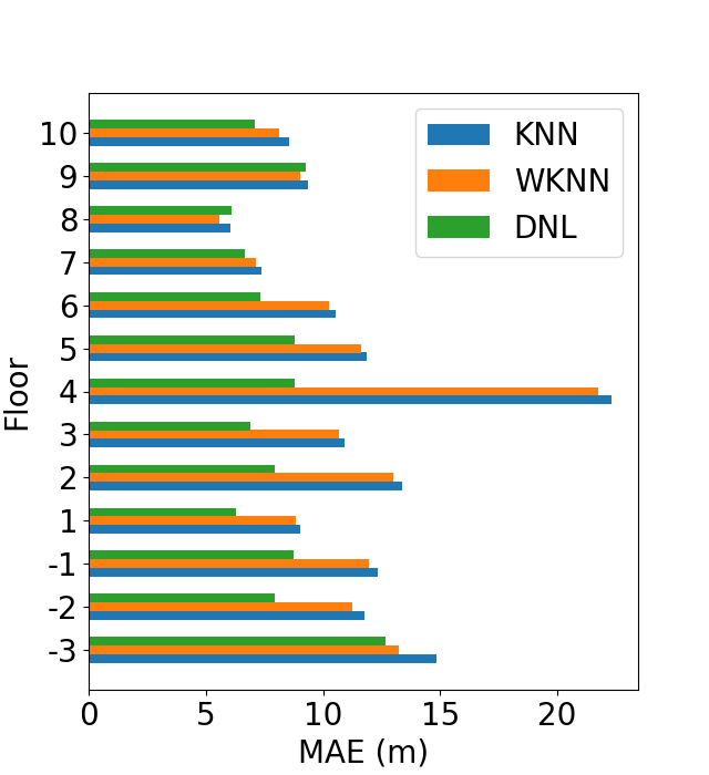
(a)

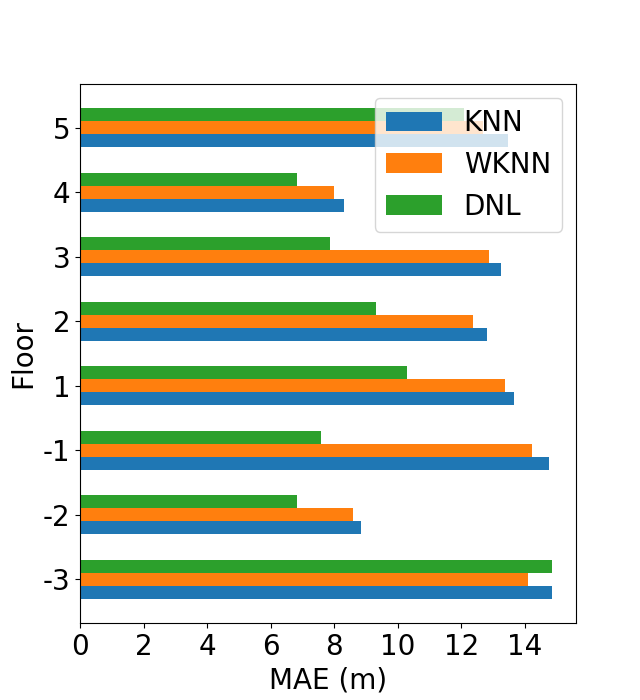
(b)

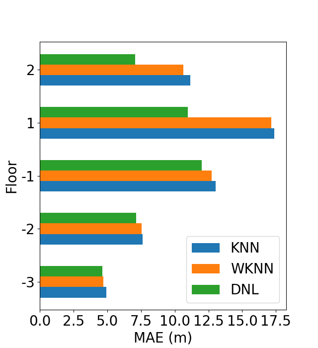
(c)

Figure 4: Comparisons of mean absolute error using different positioning algorithms on the three buildings: (a) Joycity; (b) Universal Harbor; (c) Dawan Mall.

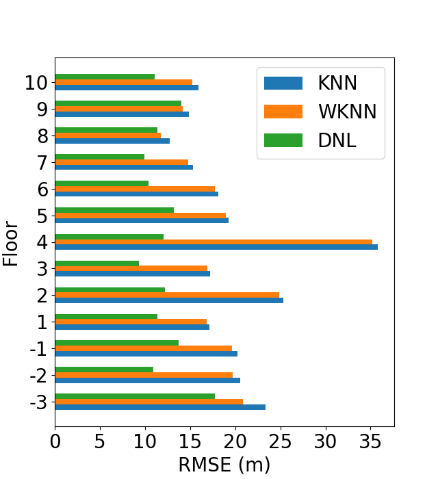
(a)

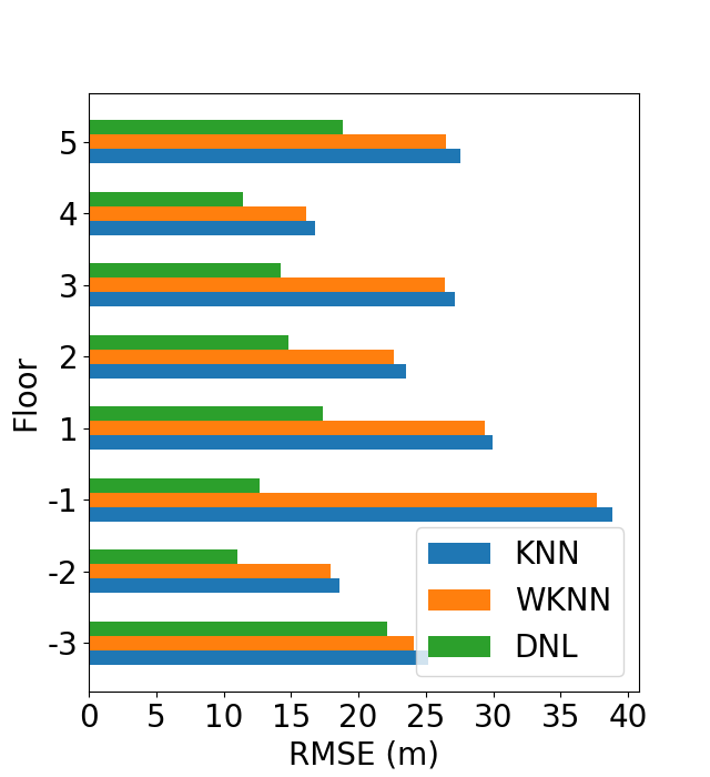
(b)

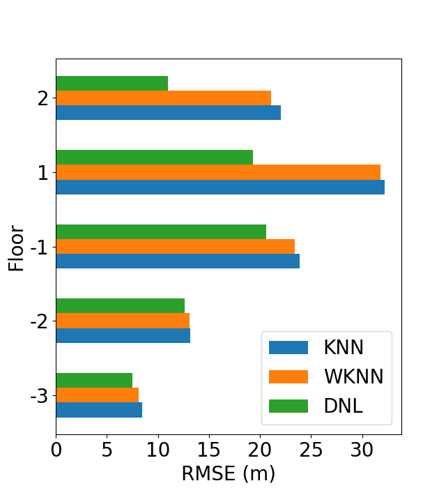
(c)

Figure 5: Comparisons of root mean squared error using different positioning algorithms on the three buildings: (a) Joycity; (b) Universal Harbor; (c) Dawan Mall.

In this section, we analyze the experimental results and evaluate the proposed model. Specially, We compare the positioning results to an unsupervised learning algorithm of k-nearest neighbors (KNN) which uses the similar strategy of WiFi neighbor selection. As illustrated previously, KNN and its variant Weighted KNN (WKNN) calculate the position of one given test point by taking the mean or the weighted mean of the selected WiFi neighbors. Such algorithms narrow down the positioning problem from the entire interested area (floor, in this study) to a local community constructed by the neighbor WiFi fingerprints. However, they do not have a learning process to infer the final location but simply calculate the mean or weighted mean of the neighbors location, which attributes to low inference ability.

Two standard positioning algorithms of KNN and WKNN were implemented for comparison in this study:

• KNN: implemented with scikit-learn K Nearest Neighbors Regression [24]; number of neighbor was set to 10; Manhattan distance was set to the distance metric.

• WKNN: similar to KNN but also set the weight as the inverse the distance in prediction.

As shown in Figure 4, using the MAE, the proposed model outperform the KNN and WKNN in 25 and 23 out of 26 cases. In detail, we can see from Table IV that the proposed model can provide a 10% to 50% reduction of the MAE in 18 (KNN) and 16 (WKNN) of the cases. Rather than simply taking the mean or the weighted mean position of the WiFi neighbors, the proposed model can well learn the WiFi neighborhood through the node features, edge features, and the topology information to make better predictions of the location.

The proposed model shows even better improvement in RMSE. As we can observe from the Table IV, the proposed model shows lower RMSE than the other two algorithms in all 26 cases. Particularly, the reduction of RMSE in most of the cases (19 cases against KNN; 15 cases against WKNN) is higher than 30%. Additionally, the proposed model provides much lower RMSE in some specific cases, particularly when the dataset has a large data volume and a large amount of detected Mac addresses. For instance, 5992 Mac addresses have been detected among 38763 FPs on the first floor of Universal harbor. Such large dataset usually contains more uncertainty and noise; however, the proposed model is able to provide approximatelly 40% less RMSE than the other two algorithms. Similar cases can also be found in Joycity and Dawan Mall from Table V and 5. This illustrates that the proposed model can provide even much smoother and more accurate predictions than the other two if the data is noisier.

Last bu not least, the cumulative positioning error of different algorithms was compared. It can be seen from Table V that the proposed model challenged KNN and WKNN in half of the cases, when using the 68 percentile of the positioning accuracy (68% of the CDF). In the remaining cases, it can be observed that the improvement of the proposed model degrade when the cases have lower data density. For example, on floor -3 and 5 in Universal Harbor, the proposed model is 18% and 28% worse than WKNN, respectively. Similar results can also be found in other floors, particularly some top floors and underground floors with less data. Nevertheless, the proposed model shows again superb performance in the 95 percentile positioning accuracy (95% of the CDF). The model can always provide much lower error than KNN and WKNN, which suggest that the proposed algorithm is more robust to outliers in large datasets like the ones observed in the middle floors or in lower density areas like the top or underground floors.

TABLE IV: Number of cases that the proposed model shows better positioning performance than KNN and WKNN

Percentage of improvement	MAE		RMSE		68%CDF		95%CDF
	KNN	WKNN	KNN	WKNN	KNN	WKNN	KNN	WKNN
0-10%	6	6	2	5	9	9	0	5
10% - 30%	9	10	5	6	7	5	9	3
30% - 50%	9	6	15	12	0	0	7	8
>50%	1	1	4	3	1	1	10	9
Total	25	23	26	26	17	15	26	25

TABLE V: Comparison of the positioning error using different algorithms

Building	Floor	MAE			RMSE			68%CDF			95%CDF
		KNN	WKNN	DNL	KNN	WKNN	DNL	KNN	WKNN	DNL	KNN	WKNN	DNL
Joycity	-3	14.84	13.24	12.67	23.37	20.88	17.72	15.47	14.41	14.05	48.65	43.19	39.00
	-2	11.76	11.25	7.94	20.54	19.71	10.94	8.39	8.20	8.01	47.76	45.30	22.04
	-1	12.33	11.96	8.76	20.23	19.65	13.76	10.59	9.95	8.44	46.93	46.22	27.00
	1	9.05	8.84	6.26	17.15	16.81	11.36	6.76	6.68	5.59	35.43	34.77	17.70
	2	13.36	13.00	7.92	25.33	24.85	12.22	8.61	8.39	7.46	62.57	60.31	24.49
	3	10.91	10.67	6.90	17.24	16.91	9.36	10.00	9.78	7.32	40.60	39.99	18.50
	4	22.33	21.74	8.80	35.83	35.17	12.07	21.97	20.44	9.43	85.42	85.35	26.23
	5	11.87	11.61	8.78	19.27	18.96	13.17	10.76	10.19	9.19	43.42	42.96	22.20
	6	10.55	10.27	7.30	18.12	17.74	10.41	8.07	7.78	7.48	45.08	43.90	19.62
	7	7.37	7.14	6.68	15.31	14.80	9.90	5.93	5.76	6.57	23.56	23.04	21.08
	8	6.06	5.59	6.08	12.72	11.73	11.38	4.87	4.78	5.60	20.24	16.07	17.13
	9	9.35	9.04	9.28	14.85	14.22	14.00	9.02	8.82	8.79	34.09	32.95	29.69
	10	8.54	8.13	7.09	15.96	15.24	11.05	6.53	6.16	6.33	37.33	36.14	26.24
Universal Harbor	-3	14.86	14.09	14.84	25.20	24.08	22.14	12.70	12.26	14.87	59.26	53.66	49.46
	-2	8.83	8.59	6.84	18.55	17.93	11.06	6.23	6.13	6.54	34.90	33.02	20.22
	-1	14.76	14.22	7.60	38.86	37.69	12.65	6.73	6.61	7.11	77.68	75.46	22.59
	1	13.65	13.37	10.29	29.91	29.33	17.34	9.37	9.23	9.24	56.25	54.77	32.10
	2	12.80	12.37	9.31	23.49	22.59	14.78	10.31	9.95	9.17	53.98	52.28	28.85
	3	13.26	12.86	7.88	27.14	26.41	14.23	7.54	7.38	7.22	69.00	67.91	22.98
	4	8.31	8.00	6.84	16.74	16.11	11.42	6.42	6.28	6.69	30.84	27.90	17.60
	5	13.47	12.69	12.10	27.55	26.53	18.85	9.60	8.57	11.98	65.35	63.82	44.16
Dawan Mall	-3	4.95	4.73	4.64	8.44	8.09	7.49	4.42	4.35	4.44	17.05	15.12	12.54
	-2	7.62	7.56	7.14	13.17	13.10	12.65	7.09	7.03	6.69	20.87	20.51	18.48
	-1	13.04	12.75	12.02	23.89	23.39	20.61	9.24	9.04	10.70	62.01	61.03	47.32
	1	17.39	17.15	10.99	32.23	31.81	19.30	12.07	11.96	9.49	78.74	78.30	37.01
	2	11.14	10.63	7.07	22.02	21.07	10.97	7.36	7.09	6.70	52.87	51.13	23.25

V Conclusions

In conclusion, we have proposed a Deep Neighborhood Learning approach to compensate the intrinsic problem of losing relational information among FPs and WAPs in conventional KNN or WKNN-based WiFi fingerprinting algorithms. For a given target FP, the proposed approach constructs a heterogeneous graph based on its local community containing the WiFi neighbor FPs and all the WAPs that can be detected within the community. A special neural network model has been designed to learn the topology information and the features from the neighborhood in the graph, and project the extracted embedding to the location of the target FP. Compared to KNN and WKNN, experiments on 3 real industrial datasets collected from 3 shopping malls, covering 26 floors in total, have shown that the proposed approach can better learn the neighborhood information and reduce the positioning error (MAE and RMSE) by 10% to 50% in most of the cases. Particularly, the DNL approach can always provide much lower RMSE and 95% percentile positioning error, being more robust to the outliers caused by the noise from huge datasets.

Our future work will be conducted from two aspects. On one hand, we will integrate the WiFi distance learning model proposed in our recent work to select better WiFi neighbors; On the other hand, we will include more information to the local community to extract even better representation of the WiFi fingerprints, such as the measurements and calculations from the inertial sensors and GNSS data.

References

- [1] Van Nee, Richard DJ. ”Multipath and multi-transmitter interference in spread spectrum communication and navigation systems.” Doctoral dissertation, Technische Universiteit Delft, Delft, The Netherlands. 1996
- [2] Liu, F., Liu, J., Yin, Y., Wang, W., Hu, D., Chen, P. and Niu, Q. ”Survey on WiFi-based indoor positioning techniques”. IET Communications, vol 14, no 9: p. 1372-1383, June 2020, doi: 10.1049/iet-com.2019.1059.
- [3] Gallo, Pierluigi, and Stefano Mangione. ”RSS-eye: Human-assisted indoor localization without radio maps.” 2015 IEEE International Conference on Communications (ICC). IEEE, 2015.
- [4] Wen, Fuxi, and Chen Liang. ”An indoor AOA estimation algorithm for IEEE 802.11 ac Wi-Fi signal using single access point.” IEEE Communications Letters 18.12 (2014): 2197-2200.
- [5] Golden, Stuart A., and Steve S. Bateman. ”Sensor measurements for Wi-Fi location with emphasis on time-of-arrival ranging.” IEEE Transactions on Mobile Computing 6.10 (2007): 1185-1198.
- [6] Danjo, Azusa, Yuki Watase, and Shinsuke Hara. ”A theoretical error analysis on indoor TOA localization scheme using unmanned aerial vehicles.” 2015 IEEE 81st Vehicular Technology Conference (VTC Spring). IEEE, 2015.
- [7] Nawaz, Haq, Ayhan Bozkurt, and Ibrahim Tekin. ”A novel power efficient asynchronous time difference of arrival indoor localization system using CC1101 radio transceivers.” Microwave and Optical Technology Letters 59.3 (2017): 550-555.
- [8] Hernández, Noelia, et al. ”Continuous space estimation: Increasing WiFi-based indoor localization resolution without increasing the site-survey effort.” Sensors 17.1 (2017): 147.
- [9] Ding, Genming, Jinbao Zhang, and Zhenhui Tan. ”Overview of received signal strength based fingerprinting localization in indoor wireless LAN environments.” 2013 5th IEEE International Symposium on Microwave, Antenna, Propagation and EMC Technologies for Wireless Communications. IEEE, 2013.
- [10] M. Hidayab, A. H. Ali and K. B. Abas Azmi, ”Wifi signal propagation at 2.4 GHz,” 2009 Asia Pacific Microwave Conference, 2009, pp. 528-531, doi: 10.1109/APMC.2009.5384182.
- [11] M. M. Atia, M. Korenberg and A. Noureldin, ”A consistent zero-configuration GPS-Like indoor positioning system based on signal strength in IEEE 802.11 networks,” Proceedings of the 2012 IEEE/ION Position, Location and Navigation Symposium, 2012, pp. 1068-1073, doi: 10.1109/PLANS.2012.6236849.
- [12] X. Wang, X. Wang, S. Mao, J. Zhang, S. C. G. Periaswamy and J. Patton, ”Indoor Radio Map Construction and Localization With Deep Gaussian Processes,” in IEEE Internet of Things Journal, vol. 7, no. 11, pp. 11238-11249, Nov. 2020, doi: 10.1109/JIOT.2020.2996564.
- [13] J. Torres-Sospedra, R. Montoliu, S. Trilles, Ó. Belmonte, and J. Huerta, “Comprehensive analysis of distance and similarity measures for wi-fi fingerprinting indoor positioning systems,” Expert Systems with Applications, vol. 42, no. 23, pp. 9263–9278, 2015
- [14] C. Li, Z. Qiu, and C. Liu, “An improved weighted K-nearest neighbor algorithm for indoor positioning,” Wireless Pers. Commun., vol. 96, no. 2, pp. 2239–2251, Sep. 2017.
- [15] R. Zhou, Y. Yang, and P. Chen, “An RSS transform—Based WKNN for indoor positioning,” Sensors, vol. 21, no. 17, p. 5685, Aug. 2021, doi: 10.3390/s21175685.
- [16] Chai ML, Li CG, Huang H. A New Indoor Positioning Algorithm of Cellular and Wi-Fi Networks[J]. Journal of Navigation, 2020, 73(3):1- 21
- [17] Feng, Y., Minghua, J., Jing, L., Xiao, Q., Ming, H., Tao, P., Xinrong, H.: ”An improved indoor localization of WiFi based on support vector machines”. International Journal of Future Generation Communication and Networking 7.5 (2014): 191-206.
- [18] Zhang, W., Wang, L., Qin, Z., Zheng, X., Sun, L., Jin, N., Shu, L.: ”INBS: An Improved Naive Bayes Simple learning approach for accurate indoor localization”. In: 2014 IEEE International Conference on Communications (ICC), pp. 148–153 (2014). https://doi.org/10.1109/ICC.2014.6883310
- [19] Chen, Z., Wang, J.: ”GROF: Indoor localization using a multiplebandwidth general regression neural network and outlier filter”. Sensors 18(11), 3723 (2018). https://doi.org/10.3390/s18113723
- [20] Shenoy, M.V., Karuppiah, A., Manjarekar, N.: ”A Lightweight ANN based Robust Localization Technique for Rapid Deployment of Autonomous Systems”. Journal of Ambient Intelligence and Humanized Computing. 1–16. https://doi.org/10.1007/s12652-019-01331-0 (2019)
- [21] Zhang, M., Fan, Z., Shibasaki, R., Song, X. Domain Adversarial Graph Convolutional Network Based on RSSI and Crowdsensing for Indoor Localization. arXiv preprint arXiv:2204.05184. 2022
- [22] Gu, Yang, Caifa Zhou, Andreas Wieser, and Zhimin Zhou. ”Trajectory estimation and crowdsourced radio map establishment from foot-mounted imus, wi-fi fingerprints, and gps positions.” IEEE sensors journal 19, no. 3 (2018): 1104-1113.
- [23] K. Xu, W. Hu, J. Leskovec, and S. Jegelka, “How powerful are graph neural networks,” in Proc. ICLR, 2019, pp. 1–17.
- [24] F. Pedregosa et al., “Scikit-learn: Machine learning in Python,” J. Mach. Learn. Res., vol. 12, pp. 2825–2830, Feb. 2011.