Average-Constrained Policy Optimization

Abstract

Reinforcement Learning (RL) with constraints is becoming an increasingly important problem for various applications. Often, the average criterion is more suitable than the discounted criterion. Yet, RL for average criterion-constrained MDPs remains a challenging problem. Algorithms designed for discounted constrained RL problems often do not perform well for the average CMDP setting. In this paper, we introduce a new policy optimization with function approximation algorithm for constrained MDPs with the average criterion. The Average-Constrained Policy Optimization (ACPO) algorithm is inspired by the famed PPO-type algorithms based on trust region methods. We develop basic sensitivity theory for average MDPs, and then use the corresponding bounds in the design of the algorithm. We provide theoretical guarantees on its performance, and through extensive experimental work in various challenging MuJoCo environments, show the superior performance of the algorithm when compared to other state-of-the-art algorithms adapted for the average CMDP setting.

1 Introduction

In recent years, reinforcement learning (RL) techniques have achieved remarkable successes on a variety of complex tasks including the game of Go [30], robotic control [22], and the real-time game StarCraft [36]. In these tasks, the agents are allowed to explore the state space and experiment with every action during training. However, in many realistic applications such as navigation robots [13, 4] and robotic assistants, considerations of safety and cost require the agent to operate with some constraints.

A standard RL formulation for learning with constraints is the constrained Markov Decision Process (CMDP) framework [12], where the agent must satisfy constraints on auxiliary costs while learning the optimal policy [42, 40]. To this end, [3] and [32] proposed algorithms for discounted MDPs with constraints. However, these deep RL (DRL) constrained policy algorithms are only suitable for the discounted setting. In many tasks such as robot locomotion or large language model deployment, we often care about maximizing the undiscounted average-rewards in the long run, which is generally considered as a more challenging objective.

Given the need for average-reward algorithms, one might posit that having the discount factor $\gamma\to 1$ in algorithms for the discounted setting would obviate the need for policy optimization algorithms specifically for the constrained average-reward setting. However, many algorithms break down when the discount factor gets too close to 1 [17, 20, 5]. Although policy optimization algorithms for the average reward case have been proposed [44, 38, 23], they cannot incorporate constraints.

In this work, we propose such a policy optimization algorithm for an average-CMDP with function approximation. Our approach is motivated by theoretical guarantees that bound the difference between the average long-run rewards or costs of different policies. We build on [3], which presents a policy improvement theorem for the discounted setting based on the trust region methods of [27]. We show that this result trivializes for the average setting and hence is not directly useful. Instead, we derive a new bound that depends on the worst-case level of “mixture" of the irreducible Markov chain associated with a policy. We then use trust region methods to provide policy degradation and constraint violation guarantees.

Motivated by these theoretical developments, we propose a novel Average-Constrained Policy Optimization (ACPO) algorithm for average-CMDPs. For experimental validation, we use several MuJoCo environments [34], train large neural network policies and demonstrate the effectiveness and superior performance of the ACPO algorithm as compared to others.

Main Contributions.

A brief summary of our work’s contributions:

• We propose ACPO, the first on-policy Deep RL algorithm with function approximation specifically designed for average-CMDPs, inspired by policy optimization algorithms.

• Our empirical results show that ACPO out-performs all state-of-the-art Deep RL algorithms such as CPO [3], PCPO [42], PPO [29], BVF-PPO [26] and ATRPO [44], that while not designed for average-CMDPs could be applied with some tweaks.

• We introduce an approximate but novel line search procedure that improves the empirical performance of our algorithm, and suggests that the same may hold for policy optimization algorithms like PPO as well.

Related Work

Learning constraint-satisfaction policies has been explored in the Deep RL literature [10]. This can either be (1) through expert annotations and demonstrations [25, 9] or, (2) by exploration with constraint satisfaction [3, 32]. While the former approach is not scalable since it requires human interventions, current state-of-the-art algorithms for the latter are not applicable to the average reward setting.

Previous work on RL with the average reward criterion has mostly attempted to extend stochastic approximation schemes for the tabular setting, such as Q-learning [1, 38], to the non-tabular setting with function approximation [39, 43]. [6] deals with online learning in a constrained MDP setting, but their aim is regret minimization or exploration, both in tabular settings. [43] provide bounds on the performance of a trust region algorithm for the the average reward setting but do not incorporate constraints.

Thus, we believe that our ACPO algorithm is the first policy optimization algorithm for CMDPs with average rewards and average constraints, and with function approximation. The algorithm, just like PPO, is practical and scalable, as seen by its superior empirical performance compared to other alternatives.

Since our work is related to CPO [3] and ATRPO [44], we highlight our work’s novelty as follows. ACPO is designed to find the optimal policy of the undiscounted average-CMDP problem directly, with an average reward objective and constraints on average cost functions. While CPO is designed for discounted CMDPs (setting $\gamma=1$ in CPO does not yield the ACPO algorithm), and though we could use it for the average case by setting $\gamma\to 1$, we shall see that empirically it has inferior performance to ACPO. Moreover, theory for CPO and ATRPO cannot be extended trivially to the ACPO algorithm, but since they are all trust region methods, they share some analysis. Several of our techniques are still unique, e.g. in Lemma 3.3, we use eigenvalues of the transition matrix to relate total variation (TV) of stationary distributions with the TV of the policies, and in Lemma A.3, we use the sublevel sets of constraints and projection inequality of Bregman divergence. We now begin with some preliminaries.

2 Preliminaries

A Markov decision process (MDP) is a tuple, ($S,A,r,P,\mu$), where $S$ is the set of states, $A$ is the set of actions, $r:S\times A\times S\to{\mathbb{R}}$ is the reward function, $P:S\times A\times S\to[0,1]$ is the transition probability function such that $P(s^{\prime}|s,a)$ is the probability of transitioning to state $s^{\prime}$ from state $s$ by taking action $a$, and $\mu:S\to[0,1]$ is the initial state distribution. A stationary policy $\pi:S\to\Delta(A)$ is a mapping from states to probability distributions over the actions, with $\pi(a|s)$ denoting the probability of selecting action $a$ in state $s$, and $\Delta(A)$ is the probability simplex over the action space $A$. We denote the set of all stationary policies by $\Pi$. For the average setting, we will make the standard assumption that the MDP is ergodic.

In reinforcement learning, we aim to select a policy $\pi$ which maximizes a performance measure, $J(\pi)$, which, for continuous control tasks is either the discounted reward criterion or the average reward approach. Below, we briefly discuss both formulations.

2.1 Discounted criterion

For a given discount factor $\gamma\in(0,1)$, the discounted reward objective is defined as

$$J_{\gamma}(\pi) :=\underset{\begin{subarray}{c}\tau\sim\pi\end{subarray}}{{\mathbb{E}}}\left[\sum_{t=0}^{\infty}\gamma^{t}r(s_{t},a_{t},s_{t+1})\right]=\frac{1}{1-\gamma}\underset{\begin{subarray}{c}s\sim d_{\pi,\gamma}\\ a\sim\pi\\ s^{\prime}\sim P(\cdot|s,a)\end{subarray}}{{\mathbb{E}}}[r(s,a,s^{\prime})]$$

where $\tau$ refers to a sample trajectory of $(s_{0},a_{0},s_{1},\cdots)$ generated when following a policy $\pi$, that is, $a_{t}\sim\pi(\cdot|s_{t})$ and $s_{t+1}\sim P(\cdot|s_{t},a_{t})\,$; $d_{\pi,\gamma}$ is the discounted occupation measure that is defined by $d_{\pi,\gamma}(s)=(1-\gamma)\sum_{t=0}^{\infty}\gamma^{t}\underset{\tau\sim\pi}{P}(s_{t}=s)$, which essentially refers to the discounted fraction of time spent in state $s$ while following policy $\pi$.

2.2 Average criterion

The average-reward objective is given by:

$$\begin{split}J(\pi)&:=\lim_{N\to\infty}\frac{1}{N}\underset{\begin{subarray}{c}\tau\sim\pi\end{subarray}}{{\mathbb{E}}}\left[\sum_{t=0}^{N-1}r(s_{t},a_{t},s_{t+1})\right]=\underset{\begin{subarray}{c}s\sim d_{\pi}\\ a\sim\pi(\cdot|s)\\ s^{\prime}\sim P(\cdot|s,a)\end{subarray}}{{\mathbb{E}}}[r(s,a,s^{\prime})],\end{split}$$ (1)

where $d_{\pi}(s):=\lim_{N\to\infty}\frac{1}{N}\sum_{t=0}^{N-1}P_{\tau\sim\pi}(s_{t}=s)$ is the stationary state distribution under policy $\pi$. The limits in $J(\pi)$ and $d_{\pi}(s)$ are guaranteed to exist under our ergodic assumption. Since the MDP is aperiodic, it can also be shown that $d_{\pi}(s)=\lim_{t\to\infty}P_{\tau\sim\pi}(s_{t}=s)$. Since we have $\lim_{\gamma\to 1}d_{\pi,\gamma}(s)\to d_{\pi}(s),\forall s$, it can be shown that $\lim_{\gamma\to 1}(1-\gamma)J_{\gamma}(\pi)=J(\pi)$.

In the average setting, we seek to keep the estimate of the state value function unbiased and hence, introduce the average-reward bias function as

$$\widebar{V}^{\pi}(s):=\underset{\begin{subarray}{c}\tau\sim\pi\end{subarray}}{{\mathbb{E}}}\left[\sum_{t=0}^{\infty}(r(s_{t},a_{t},s_{t+1})-J(\pi))\;\bigg{|}\;s_{0}=s\right]$$

and the average-reward action-bias function as

$$\widebar{Q}^{\pi}(s,a):=\underset{\begin{subarray}{c}\tau\sim\pi\end{subarray}}{{\mathbb{E}}}\bigg{[}\sum_{t=0}^{\infty}(r(s_{t},a_{t},s_{t+1})- J(\pi))\;\bigg{|}\;s_{0}=s,a_{0}=a\bigg{]}.$$

Finally, define the average-reward advantage function as $\widebar{A}^{\pi}(s,a):=\widebar{Q}^{\pi}(s,a)-\widebar{V}^{\pi}(s)$.

2.3 Constrained MDPs

A constrained Markov decision process (CMDP) is an MDP augmented with constraints that restrict the set of allowable policies for that MDP. Specifically, we augment the MDP with a set $C$ of auxiliary cost functions, $C_{1},\cdots,C_{m}$ (with each function $C_{i}:S\times A\times S\to{\mathbb{R}}$ mapping transition tuples to costs, just like the reward function), and bounds $l_{1},\cdots,l_{m}$. Similar to the value functions being defined for the average reward criterion, we define the average cost objective with respect to the cost function $C_{i}$ as

$$J_{C_{i}}(\pi):=\lim_{N\to\infty}\frac{1}{N}\underset{\begin{subarray}{c}\tau\sim\pi\end{subarray}}{{\mathbb{E}}}\left[\sum_{t=0}^{N-1}C_{i}(s_{t},a_{t},s_{t+1})\right]=\underset{\begin{subarray}{c}s\sim d_{\pi}\\ a\sim\pi\\ s^{\prime}\sim P(\cdot|s,a)\end{subarray}}{{\mathbb{E}}}[C_{i}(s,a,s^{\prime})].$$ (2)

where $J_{C_{i}}$ will be referred to as the average cost for constraint $C_{i}$. The set of feasible stationary policies for a CMDP then is given by $\Pi_{C}:=\left\{\pi\in\Pi\;:\;J_{C_{i}}(\pi)\leq l_{i},{\;\;\forall\;}i\in\{1,\cdots,M\}\right\}$. The goal is to find a policy $\pi^{\star}$ such that $\pi^{\star}\in\arg\max_{\pi\in\Pi_{C}}J(\pi).$

However, finding an exact $\pi^{\star}$ is infeasible for large-scale problems. Instead, we aim to derive an iterative policy improvement algorithm that given a current policy, improves upon it by approximately maximizing the increase in the reward, while not violating the constraints by too much and not being too different from the current policy.

Lastly, analogous to $\widebar{V}^{\pi}$, $\widebar{Q}^{\pi}$, and $\widebar{A}^{\pi}$, we define similar quantities for the cost functions $C_{i}(\cdot)$, and denote them by $\widebar{V}_{C_{i}}^{\pi}$, $\widebar{Q}_{C_{i}}^{\pi}$, and $\widebar{A}_{C_{i}}^{\pi}$.

2.4 Policy Improvement for discounted CMDPs

In many on-policy constrained RL problems, we improve policies iteratively by maximizing a predefined function within a local region of the current best policy [32, 3, 42, 31]. [3] derived a policy improvement bound for the discounted CMDP setting as:

$$J_{\gamma}(\pi_{k+1})-J_{\gamma}(\pi_{k})\geq\frac{1}{1-\gamma}\underset{\begin{subarray}{c}s\sim d^{\pi_{k}}\\ a\sim\pi_{k+1}\end{subarray}}{{\mathbb{E}}}\left[A_{\gamma}^{\pi_{k}}(s,a)-\frac{2\gamma\epsilon^{\pi_{k+1}}}{1-\gamma}D_{TV}(\pi_{k+1}||\pi_{k})[s]\right],$$ (3)

where $A_{\gamma}^{\pi_{k}}$ is the discounted version of the advantage function, $\epsilon^{\pi_{k+1}}:=\max_{s}|{\mathbb{E}}_{a\sim\pi_{k+1}}[A_{\gamma}^{\pi_{k}}(s,a)]|$, and $D_{TV}(\pi_{k+1}||\pi_{k})[s]=(1/2)\sum_{a}\left|\pi_{k+1}(a|s)-\pi_{k}(a|s)\right|$ is the total variational divergence between $\pi_{k+1}$ and $\pi_{k}$ at $s$. These results laid the foundations for on-policy constrained RL algorithms [41, 37].

However, Equation (3) does not generalize to the average setting ($\gamma\to 1$) (see Appendix A.1). In the next section, we will derive a policy improvement bound for the average case and present an algorithm based on trust region methods, which will generate almost-monotonically improving iterative policies. Proofs of theorems and lemmas, if not already given, are available in Appendix A.

3 ACPO: The Average-Constrained Policy Optimization Algorithm

In this section, we present the main results of our work. For conciseness, we denote by $d_{\pi}\in{\mathbb{R}}^{|S|}$ the column vector whose components are $d_{\pi}(s)$ and $P_{\pi}\in{\mathbb{R}}^{|S|\times|S|}$ to be the state transition probability matrix under policy $\pi$.

3.1 Policy Improvement for the Average-CMDP

Let $\pi^{\prime}$ be the policy obtained via some update rule from the current policy $\pi$. Analogous to the discounted setting of a CMDP, we would like to characterize the performance difference $J(\pi^{\prime})-J(\pi)$ by an expression which depends on $\pi$ and some divergence metric between the two policies. [44] give such a lemma.

Lemma 3.1.

[44] Under the unichain assumption of the underlying Markov chain, for any stochastic policies $\pi$ and $\pi^{\prime}$:

$$J(\pi^{\prime})-J(\pi)=\underset{\begin{subarray}{c}s\sim d_{\pi^{\prime}}\\ a\sim\pi^{\prime}\end{subarray}}{{\mathbb{E}}}\left[\widebar{A}^{\pi}(s,a)\right].$$ (4)

Note that this difference depends on the stationary state distribution obtained from the new policy, $d_{\pi^{\prime}}$. This is computationally impractical as we do not have access to this $d_{\pi^{\prime}}$. Fortunately, by use of the following lemma we can show that if $d_{\pi}$ and $d_{\pi^{\prime}}$ are “close” with respect to some metric, we can approximate Eq. (4) using samples from $d_{\pi}$.

Lemma 3.2.

Under the unichain assumption, for any stochastic policies $\pi$ and $\pi^{\prime}$ we have:

$$\left|J(\pi^{\prime})-J(\pi)-\underset{\begin{subarray}{c}s\sim d_{\pi}\\ a\sim\pi^{\prime}\end{subarray}}{{\mathbb{E}}}\left[\widebar{A}^{\pi}(s,a)\right]\right|\leq 2\epsilon D_{\text{TV}}(d_{\pi^{\prime}}\parallel d_{\pi})\quad\text{where}\quad\epsilon=\max_{s}\big{|}\underset{\begin{subarray}{c}a\sim\pi^{\prime}\end{subarray}}{{\mathbb{E}}}[\widebar{A}^{\pi}(s,a)]\big{|}.$$ (5)

See Appendix A.1 for proof. Lemma 3.2 implies $J(\pi^{\prime})\approx J(\pi)+\underset{\begin{subarray}{c}\end{subarray}}{{\mathbb{E}}}[\widebar{A}^{\pi}(s,a)]$ when $d_{\pi}$ and $d_{\pi^{\prime}}$ are “close”. Now that we have established this approximation, we need to study the relation of how the actual change in policies affects their corresponding stationary state distributions. For this, we turn to standard analysis of the underlying Markov chain of the CMDP.

Under the ergodic assumption, we have that $P_{\pi}$ is irreducible and hence its eigenvalues $\{\lambda_{\pi,i}\}_{i=1}^{|S|}$ are such that $\lambda_{\pi,1}=1$ and $\lambda_{\pi,i\neq 1}<1$. For our analysis, we define $\sigma^{\pi}=\max_{i\neq 1}\,(1-\lambda_{\pi,i})^{-1/2}$, and from [21] and [8], we connect $\{\lambda_{\pi,i}\}_{i=1}^{|S|}$ to the sensitivity of the stationary distributions to changes in the policy using the result below.

Lemma 3.3.

Under the ergodic assumption, the divergence between the stationary distributions $d_{\pi}$ and $d_{\pi^{\prime}}$ is upper bounded as:

$$D_{\text{TV}}(d_{\pi^{\prime}}\parallel d_{\pi})\leq\sigma^{\star}\underset{\begin{subarray}{c}s\sim d_{\pi}\end{subarray}}{{\mathbb{E}}}[D_{\text{TV}}(\pi^{\prime}\parallel\pi)[s]]\quad\text{where}\quad\sigma^{\star}=\max_{\pi}\sigma^{\pi}.$$ (6)

See Appendix A.1 for proof. This bound is tighter and easier to compute than the one given by [44], which replaces $\sigma^{\star}$ by $\kappa^{\star}=\max_{\pi}\kappa^{\pi}$, where $\kappa^{\pi}$ is known as Kemeny’s constant [19, 11, 16]. It is interpreted as the expected number of steps to get to any goal state, where the expectation is taken with respect to the stationary-distribution of those states.

Combining the bounds in Lemma 3.2 and Lemma 3.3 gives us the following result:

Proposition 3.4.

Under the ergodic assumption, the following bounds hold for any stochastic policies $\pi$ and $\pi^{\prime}$:

$$L_{\pi}^{-}(\pi^{\prime})\leq J(\pi^{\prime})-J(\pi)\leq L_{\pi}^{+}(\pi^{\prime})$$ (7)

where

$$L_{\pi}^{\pm}(\pi^{\prime})=\underset{\begin{subarray}{c}s\sim d_{\pi}\\ a\sim\pi^{\prime}\end{subarray}}{{\mathbb{E}}}\left[\widebar{A}^{\pi}(s,a)\right]\pm 2\nu\underset{\begin{subarray}{c}s\sim d_{\pi}\end{subarray}}{{\mathbb{E}}}[D_{\text{TV}}(\pi^{\prime}\parallel\pi)[s]]\quad\text{and}\quad\nu=\sigma^{\star}\max_{s}\big{|}\underset{\begin{subarray}{c}a\sim\pi^{\prime}\end{subarray}}{{\mathbb{E}}}[\widebar{A}^{\pi}(s,a)]\big{|}.$$

It is interesting to compare the inequalities of Equation (7) to Equation (4). The term $\underset{\begin{subarray}{c}\end{subarray}}{{\mathbb{E}}}[\widebar{A}^{\pi}(s,a)]$ in Prop. 3.4 is somewhat of a surrogate approximation to $J(\pi^{\prime})-J(\pi)$, in the sense that it uses $d_{\pi}$ instead of $d_{\pi^{\prime}}$. As discussed before, we do not have access to $d_{\pi^{\prime}}$ since the trajectories of the new policy are not available unless the policy itself is updated. This surrogate is a first order approximation to $J(\pi^{\prime})-J(\pi)$ in the parameters of $\pi^{\prime}$ in a neighborhood around $\pi$ [18]. Hence, Eq. (7) can be viewed as bounding the worst-case approximation error.

Extending this discussion to the cost function of our CMDP, similar expressions follow immediately.

Corollary 3.5.

For any policies $\pi^{\prime},\pi$, and any cost function $C_{i}$, the following bound holds:

$$M_{\pi}^{-}(\pi^{\prime})\leq J_{C_{i}}(\pi^{\prime})-J_{C_{i}}(\pi)\leq M_{\pi}^{+}(\pi^{\prime})$$ (8)

where

$$M_{\pi}^{\pm}(\pi^{\prime})=\underset{\begin{subarray}{c}s\sim d_{\pi}\\ a\sim\pi^{\prime}\end{subarray}}{{\mathbb{E}}}\left[\widebar{A}_{C_{i}}^{\pi}(s,a)\right]\pm 2\nu_{C_{i}}\underset{\begin{subarray}{c}s\sim d_{\pi}\end{subarray}}{{\mathbb{E}}}[D_{\text{TV}}(\pi^{\prime}\parallel\pi)[s]]\quad\text{and}\quad\nu_{C_{i}}=\sigma^{\star}\max_{s}\big{|}\underset{\begin{subarray}{c}a\sim\pi^{\prime}\end{subarray}}{{\mathbb{E}}}[\widebar{A}_{C_{i}}^{\pi}(s,a)]\big{|}.$$

Until now, we have been dealing with bounds given with regards to the TV divergence of the policies. However, in practice, bounds with respect to the KL divergence of policies is more commonly used [27, 28, 24]. From Pinsker’s and Jensen’s inequalities, we have that

$$\underset{\begin{subarray}{c}s\sim d_{\pi}\end{subarray}}{{\mathbb{E}}}\big{[}D_{\text{TV}}(\pi^{\prime}\parallel\pi)[s]\big{]} \leq\sqrt{\underset{\begin{subarray}{c}s\sim d_{\pi}\end{subarray}}{{\mathbb{E}}}\big{[}D_{\text{KL}}\left(\pi^{\prime}\middle\|\pi\right)][s]\big{]}/2}.$$ (9)

We can thus use Eq. (9) in the bounds of Proposition 3.4 and Corollary 3.5 to make policy improvement guarantees, i.e., if we find updates such that $\pi_{k+1}\in\operatorname*{arg\,max}_{\pi}L_{\pi_{k}}^{-}(\pi)$, then we will have monotonically increasing policies as, at iteration $k$, $\underset{\begin{subarray}{c}s\sim d_{\pi_{k}},a\sim\pi\end{subarray}}{{\mathbb{E}}}[\widebar{A}^{\pi_{k}}(s,a)]=0$, $\underset{\begin{subarray}{c}s\sim d_{\pi_{k}}\end{subarray}}{{\mathbb{E}}}[D_{\text{KL}}\left(\pi\middle\|\pi_{k}\right)[s]]=0$ for $\pi=\pi_{k}$, implying that $J(\pi_{k+1})-J(\pi_{k})\geq 0$. However, this sequence does not guarantee constraint satisfaction at each iteration, so we now turn to trust region methods to incorporate constraints, do policy improvement and provide safety guarantees.

3.2 Trust Region Based Approach

For large or continuous state and action CMDPs, solving for the exact optimal policy is impractical. However, trust region-based policy optimization algorithms have proven to be effective for solving such problems [27, 28, 29, 2]. For these approaches, we usually consider some parameterized policy class $\Pi_{\Theta}=\{\pi_{\theta}:\theta\in\Theta\}$ for tractibility. In addition, for CMDPs, we also require the policy iterates to be feasible, so instead of optimizing just over $\Pi_{\Theta}$, we optimize over $\Pi_{\Theta}\cap\Pi_{C}$. However, it is much easier to solve the above problem if we introduce hard constraints, rather than limiting the set to $\Pi_{\Theta}\cap\Pi_{C}$. Therefore, we now introduce the ACPO algorithm, which is inspired by the trust region formulations above as the following optimization problem:

$$\underset{\pi\in\Pi_{\Theta}}{\text{maximize}} \quad\underset{\begin{subarray}{c}s\sim d_{\pi_{\theta_{k}}}\\ a\sim\pi\end{subarray}}{{\mathbb{E}}}[\widebar{A}^{\pi_{\theta_{k}}}(s,a)]$$ (10)

s.t. $$\qquad J_{C_{i}}(\pi_{\theta_{k}})+\underset{\begin{subarray}{c}s\sim d_{\pi_{\theta_{k}}}\\ a\sim\pi\end{subarray}}{{\mathbb{E}}}[\widebar{A}_{C_{i}}^{\pi_{\theta_{k}}}(s,a)]\leq l_{i},\;\;\;{\;\;\forall\;}i$$

$$\qquad\bar{D}_{\text{KL}}(\pi\parallel\pi_{\theta_{k}})\leq\delta$$

where $\bar{D}_{\text{KL}}(\pi\parallel\pi_{\theta_{k}}):=\underset{\begin{subarray}{c}s\sim d_{\pi_{\theta_{k}}}\end{subarray}}{{\mathbb{E}}}[D_{\text{KL}}\left(\pi\middle\|\pi_{\theta_{k}}\right)[s]]$, $\widebar{A}^{\pi_{\theta_{k}}}(s,a)$ is the average advantage function defined earlier, and $\delta>0$ is a step size. We use this form of updates as it is an approximation to the lower bound given in Proposition 3.4 and the upper bound given in Corollary 3.5.

In most cases, the trust region threshold for formulations like Eq. (10) are heuristically motivated. We now show that it is quantitatively motivated and comes with a worst case performance degradation and constraint violation. Proof is in Appendix A.2.

Theorem 3.6.

Let $\pi_{\theta_{k+1}}$ be the optimal solution to Eq. (10) for some $\pi_{\theta_{k}}\in\Pi_{\Theta}$. Then, we have

$$J(\pi_{\theta_{k+1}})-J(\pi_{\theta_{k}})\geq -\sqrt{2(\delta+V_{max})}\nu^{\pi_{\theta_{k+1}}}$$ (11)

$$\text{and}\;\;J_{C_{i}}(\pi_{\theta_{k+1}})\leq l_{i} +\sqrt{2(\delta+V_{max})}\nu^{\pi_{\theta_{k+1}}}_{C_{i}}{\;\;\forall\;}i,$$ (12)

where $\nu^{\pi_{\theta_{k+1}}}=\sigma^{\pi_{\theta_{k+1}}}\max_{s}\big{|}\underset{\begin{subarray}{c}a\sim\pi_{\theta_{k+1}}\end{subarray}}{{\mathbb{E}}}[\widebar{A}^{\pi_{\theta_{k}}}(s,a)]\big{|}$, $\nu^{\pi_{\theta_{k+1}}}_{C_{i}}=\sigma^{\pi_{\theta_{k+1}}}\max_{i,s}\big{|}\underset{\begin{subarray}{c}a\sim\pi_{\theta_{k+1}}\end{subarray}}{{\mathbb{E}}}[\widebar{A}_{C_{i}}^{\pi_{\theta_{k}}}(s,a)]\big{|}$, $V_{max}=\max_{i}\beta_{i}^{2}$,  and  $\beta_{i}=[J_{C_{i}}(\pi_{\theta_{k}})-l_{i}]_{+}$.

Remark 3.7. Note that if the constraints are ignored (by setting $V_{max}=0$), then this bound is tighter than given in [44] for the unconstrained average-reward setting.

However, the update rule of Eq. (10) is difficult to implement in practice as it takes steps that are too small, which degrades convergence. In addition, it requires the exact knowledge of $\widebar{A}^{\pi_{\theta_{k}}}(s,a)$ which is computationally infeasible for large-scale problems. In the next section, we will introduce a specific sampling-based practical algorithm to alleviate these concerns.

4 Practical Implementation of ACPO

In this section, we introduce a practical version of the ACPO algorithm with a principle recovery method. With a small step size $\delta$, we can approximate the reward function and constraints with a first order expansion, and approximate the KL divergence constraint with a second order expansion. This gives us a new optimization problem which can be solved exactly using Lagrangian duality.

4.1 An Implementation of ACPO

Since we are working with a parameterized class, we shall now overload notation to use $\theta_{k}$ as the policy at iteration $k$, i.e., $\theta_{k}\equiv\pi_{\theta_{k}}$. In addition, we use $g$ to denote the gradient of the advantage function objective, $a_{i}$ to denote the gradient of the advantage function of the cost $C_{i}$, $H$ as the Hessian of the KL-divergence. Formally,

$$g:=\nabla_{\theta}\underset{\begin{subarray}{c}\begin{subarray}{c}s\sim d_{\theta_{k}}\\ a\sim\theta\end{subarray}\end{subarray}}{{\mathbb{E}}}[\widebar{A}^{\theta_{k}}(s,a)]\Bigr{|}_{\theta=\theta_{k}},\quad a_{i}:=\nabla_{\theta}\underset{\begin{subarray}{c}\begin{subarray}{c}s\sim d_{\theta_{k}}\\ a\sim\theta\end{subarray}\end{subarray}}{{\mathbb{E}}}[\widebar{A}^{\theta_{k}}_{C_{i}}(s,a)]\Bigr{|}_{\theta=\theta_{k}},\quad H:=\nabla^{2}_{\theta}\underset{\begin{subarray}{c}s\sim d_{\theta_{k}}\end{subarray}}{{\mathbb{E}}}\big{[}D_{\text{KL}}\left(\theta\middle\|\theta_{k}\right))[s]\big{]}\Bigr{|}_{\theta=\theta_{k}}.$$

In addition, let $c_{i}:=J_{C_{i}}(\theta_{k})-l_{i}$. The approximation to the problem in Eq. (10) is:

$$\max_{\theta} g^{T}(\theta-\theta_{k})\quad\text{s.t. }\quad c_{i}+a_{i}^{T}(\theta-\theta_{k})\leq 0,{\;\;\forall\;}i\quad\text{and}\quad\tfrac{1}{2}(\theta-\theta_{k})^{T}H(\theta-\theta_{k})\leq\delta.$$ (13)

This is a convex optimization problem in which strong duality holds, and hence it can be solved using a Lagrangian method. The update rule for the dual problem then takes the form

$$\theta_{k+1}=\theta_{k}+\frac{1}{\lambda^{\star}}H^{-1}\left(g-A\mu^{\star}\right).$$ (14)

where $\lambda^{\star}$ and $\mu^{\star}$ are the Lagrange multipliers satisfying the dual

$$\max_{\begin{subarray}{c}\lambda\geq 0\\ \mu\succeq 0\end{subarray}}\frac{-1}{2\lambda}\left(g^{T}H^{-1}g-2r^{T}\mu+\mu^{T}S\mu\right)+\mu^{T}c-\frac{\lambda\delta}{2},$$ (15)

with $r:=g^{T}H^{-1}A$, $S:=A^{T}H^{-1}A$, $A:=[a_{1},\cdots,a_{m}]$, and $c:=[c_{1},\cdots,c_{m}]^{T}$.

4.2 Feasibility and Recovery

The approximation regime described in Eq. (13) requires $H$ to be invertible. For large parametric policies, $H$ is computed using the conjugate gradient method as in [27]. However, in practice, using this approximation along with the associated statistical sampling errors, there might be potential violations of the approximate constraints leading to infeasible policies.

To rectify this, for the case where we only have one constraint, one can recover a feasible policy by applying a recovery step inspired by the TRPO update on the cost surrogate as:

$$\theta_{k+1/2}=\theta_{k}-\sqrt{2\delta}\bigg{[}t\cdot\frac{H^{-1}a}{\sqrt{a^{T}H^{-1}a}}+(1-t)\cdot\frac{H^{-1}g}{\sqrt{g^{T}H^{-1}g}}\bigg{]}$$ (16)

where $t\in[0,1]$. Contrasting with the policy recovery update of [3] which only uses the cost advantage function gradient $a$, we introduce the reward advantage function gradient $g$ as well. This choice is to ensure recovery while simultaneously balancing the “regret” of not choosing the best (in terms of the objective value) policy $\pi_{k}$. In other words, we wish to find a policy $\pi_{k+1/2}$ as close to $\pi_{k}$ in terms of their objective function values. We follow up this step with a simple linesearch to find feasible $\pi_{k+1}$. Based on this, Algorithm 1 provides a basic outline of ACPO. For more details of the algorithm, see Appendix A.3.

Algorithm 1 Average-Constrained Policy Optimization (ACPO)

1:  Input: Initial random policy $\pi_{0}\in\Pi_{\theta}$

2:  for $k=0,1,2,...,K$ do

3:     Sample a set of trajectories $\Omega$ using $\pi_{k}=\pi_{\theta_{k}}$

4:     Find estimates of $g,a,H,c$ using $\Omega$

5:     if a feasible solution to Equation (13) exists then

6:        Solve dual problem in Equation (15) for $\lambda^{\star}_{k},\mu^{\star}_{k}$

7:        Find policy update $\pi_{k+1}$ with Equation (14)

8:     else

9:        Find recovery policy $\pi_{k+1/2}$ with Equation (16)

10:        Obtain $\pi_{k+1}$ by linesearch till approximate constraint satisfaction of Equation (13)

11:     end if

12:  end for

Average Rewards:
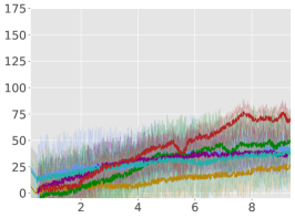
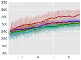
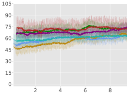
                    Average Constraint values:                

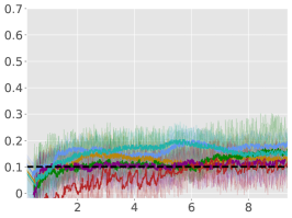
(a) Ant Gather

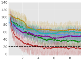
(b) Bottleneck

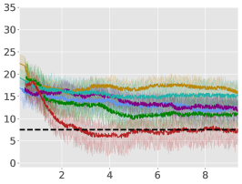
(c) Grid

Figure 1: The average reward and constraint cost function values vs iterations (in $10^{4}$) learning curves for some algorithm-task pairs. Solid lines in each figure are the empirical means, while the shaded area represents 1 standard deviation, all over 5 runs. The dashed line in constraint plots is the constraint threshold $l$. ATRPO and PPO are tested with constraints, which are included in their Lagrangian formulation. Additional results are available in Appendix A.6.

5 Empirical Results

We conducted a series of experiments to evaluate the relative performance of the ACPO algorithm and answer the following questions: (i) Does ACPO learn a sequence of constraint satisfying policies while maximizing the average reward in the long run? (ii) How does ACPO compare with the already existing constraint policy optimization algorithms which are applied with a large discount factor? (iii) What are the factors that affect the performance of ACPO?

We work with the MuJoCo environments to train the various learning agent on the following tasks - Gather, Circle, Grid, and Bottleneck tasks (see Figure 3 in Appendix A.6.1 for more details on the environments). For our experiments we only work with a single constraint with policy recovery using Eq. (16) (this is only a computational limitation; ACPO in principle can handle multiple constraints). We compare ACPO with the following baseline algorithms: CPO [3], ATRPO [44], PCPO [42] (a close variant of CPO), BVF-PPO [26] and PPO [29].

Although ATRPO and PPO originally do not incorporate constraints, for fair comparison, we introduce constraints using a Lagrangian. Also, CPO, PCPO and PPO are compared with $\gamma=0.999$. See Appendix A.5 for more details.

5.1 Evaluation Details and Protocol

For the Gather and Circle tasks we test two distinct agents: a point-mass ($S\subseteq{\mathbb{R}}^{9},A\subseteq{\mathbb{R}}^{2}$), and an ant robot ($S\subseteq{\mathbb{R}}^{32},A\subseteq{\mathbb{R}}^{8}$). The agent in the Bottleneck task in $S\subseteq{\mathbb{R}}^{71},A\subseteq{\mathbb{R}}^{16}$, and for the Grid task is $S\subseteq{\mathbb{R}}^{96},A\subseteq{\mathbb{R}}^{4}$. We use two hidden layer neural networks to represent Gaussian policies for the tasks. For Gather and Circle, size is (64,32) for both layers, and for Grid and Bottleneck the layer sizes are (16,16) and (50,25). We set the step size $\delta$ to $10^{-4}$, and for each task, we conduct 5 runs to get the mean and standard deviation for reward objective and cost constraint values during training. We train CPO, PCPO, and PPO with the discounted objective, however, evaluation and comparison with BVF-PPO, ATRPO and ACPO is done using the average reward objective (this is a standard evaluation scheme [27, 41, 37]).

For each environment, we train an agent for $10^{5}$ steps, and for every $10^{3}$ steps, we instantiate 10 evaluation trajectories with the current (deterministic) policy. For each of these trajectories, we calculate the trajectory average reward for the next $10^{3}$ steps and finally report the total average-reward as the mean of these 10 trajectories. Learning curves for the algorithms are compiled in Figure 1 (for Point-Circle, Point-Gather, and Ant-Circle see Appendix A.6).

Since there are two objectives (rewards in the objective and costs in the constraints), we show the plots which maximize the reward objective while satisfying the cost constraint. See Appendix A.4 and A.5 for more details.

5.2 Performance Analysis

From Figure 1, we can see that ACPO is able to improve the reward objective while having approximate constraint satisfaction on all tasks. In particular, ACPO is the only algorithm that best learns almost-constraint-satisfying maximum average-reward policies across all tasks: in a simple Gather environment, ACPO is able to almost exactly track the cost constraint values to within the given threshold $l$; however, for the high dimensional Grid and Bottleneck environments we have more constraint violations due to complexity of the policy behavior. Regardless, in these environments, ACPO still outperforms all other baselines with less average constraint violation, while maintaining similar if not better average-reward performance.

ACPO vs. CPO/PCPO.

For the Point-Gather environment (see Figure 4), we see that initially ACPO and CPO/PCPO give relatively similar performance, but eventually ACPO improves over CPO and PCPO by 52.5% and 36.1% on average-rewards respectively. This superior performance does not come with more constraint violation. The Ant-Gather environment particularly brings out the effectiveness of ACPO where it shows 41.1% and 61.5% improvement over CPO and PCPO respectively, while satisfying the constraint. In the high dimensional Bottleneck and Grid environments, ACPO is particularly quick at optimizing for low constraint violations, while improving over PCPO and CPO in terms of average-reward.

ACPO vs Lagrangian ATRPO/PPO.

One could suppose to use the state of the art unconstrained policy optimization algorithms with a Lagrangian formulation to solve the average-rewards CMDP problem in consideration, but we see that such an approach, although principled in theory, does not give satisfactory empirical results. This can be particularly seen in the Ant-Circle, Ant-Gather, Bottleneck, and Grid environments, where Lagrangian ATRPO and PPO give the least rewards, while not even satisfying the constraints. If ATRPO and PPO were used without the Lagrangian (i.e. constraints are ignored), one would see higher rewards but even worse constraint violations, which are not useful for solving the average-reward CMDP problem. Hence, we do not include those results.

ACPO vs BVF-PPO.

BVF-PPO is a whole different formulation than the other baselines, as it translates the cumulative cost constraints into state-based constraints, which results in an almost-safe policy improvement method which maximizes returns at every step. However, we see that this approach fails to satisfy the constraints even in the moderately difficult Ant Gather environment, let alone the high dimensional Bottleneck and Grid environments. On the other hand, ACPO performs the best among all baselines in these three environments.

5.3 Dependence of the Recovery Regime

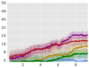
(a) Rewards

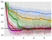
(b) Costs

Figure 2: Comparison of performance of ACPO with different values of the hyperparameter $t$ in the Point-Circle environment. X-axis is iterations in $10^{4}$. See Appendix A.6 for more details.

In Equation (16) we introduced a hyperparameter $t$, which provides for an intuitive trade-off as follows: either we purely decrease the constraint violations ($t=1$), or we decrease the average-reward ($t=0$), which consequently decreases the constraint violation. The latter formulation is principled in that if we decrease rewards, we are bound to decrease constraints violation due to the nature of the environments. Figure 2 shows the experiments we conducted with varying $t\in\{0,0.25,5,0.75,1\}$. With $t=1$, we obtain the same recovery scheme as that of [3]. Our results show that this scheme does not lead to the best performance, and that $t=0.75$ and $t=1$ perform the best across all tasks.

6 Conclusion

In this paper, we studied the problem of learning policies that maximize average-rewards for a given CMDP with average-cost constraints. We showed that the current algorithms with state-of-the-art performance and constraint violation bounds for the discounted setting do not generalize to the average setting. We then proposed a new algorithm, the Average-Constrained Policy Optimization (ACPO) that is of course directly inspired by the PPO class of algorithms but based on theoretical sensitivity-type bounds for average-CMDPs we derive, and use in designing the algorithm. Our experimental results on a range of MuJoCo environments (including some high dimensional ones) show the effectiveness of ACPO on average CMDP RL problems, as well as its superior performance vis-a-vis some current alternatives. A possible direction for future work is implementation of ACPO to fully exploit the parallelization potential.

Appendix A Appendix

A.1 Proofs

Lemma A.1 (Trivialization of Discounted Criterion Bounds).

Consider the policy performance bound of [3], which says that for any two stationary policies $\pi$ and $\pi^{\prime}$:

$$J_{\gamma}(\pi^{\prime})-J_{\gamma}(\pi)\geq\frac{1}{1-\gamma}\left[\underset{\begin{subarray}{c}\begin{subarray}{c}s\sim d_{\pi,\gamma}\\ a\sim\pi^{\prime}\end{subarray}\end{subarray}}{{\mathbb{E}}}[A_{\gamma}^{\pi}(s,a)]-\frac{2\gamma\epsilon^{\gamma}}{1-\gamma}\underset{\begin{subarray}{c}s\sim d_{\pi,\gamma}\end{subarray}}{{\mathbb{E}}}D_{\text{TV}}(\pi^{\prime}\parallel\pi)[s]\right]$$ (17)

where $\epsilon^{\gamma}=\max_{s}\left|\underset{\begin{subarray}{c}a\sim\pi^{\prime}\end{subarray}}{{\mathbb{E}}}[A_{\gamma}^{\pi}(s,a)]\right|$. Then, the right hand side times $1-\gamma$ goes to negative infinity as $\gamma\to 1$.

Proof.

Since $d_{\pi,\gamma}$ approaches the stationary distribution $d_{\pi}$ as $\gamma\to 1$, we can multiply the right hand side of (17) by $(1-\gamma)$ and take the limit which gives us:

$$\lim_{\gamma\to 1}\left(\underset{\begin{subarray}{c}\begin{subarray}{c}s\sim d_{\pi,\gamma}\\ a\sim\pi^{\prime}\end{subarray}\end{subarray}}{{\mathbb{E}}}[A_{\gamma}^{\pi}(s,a)]\pm\frac{2\gamma\epsilon^{\gamma}}{1-\gamma}\underset{\begin{subarray}{c}s\sim d_{\pi,\gamma}\end{subarray}}{{\mathbb{E}}}D_{\text{TV}}(\pi^{\prime}\parallel\pi)[s]\right)$$

$$= \underset{\begin{subarray}{c}\begin{subarray}{c}s\sim d_{\pi}\\ a\sim\pi^{\prime}\end{subarray}\end{subarray}}{{\mathbb{E}}}[\widebar{A}^{\pi}(s,a)]-2\epsilon\underset{\begin{subarray}{c}s\sim d_{\pi}\end{subarray}}{{\mathbb{E}}}\big{[}D_{\text{TV}}(\pi^{\prime}\parallel\pi)[s]\big{]}\cdot\lim_{\gamma\to 1}\frac{\gamma}{1-\gamma}$$

$$= -\infty$$

Here $\epsilon=\max_{s}\left|\underset{\begin{subarray}{c}a\sim\pi^{\prime}\end{subarray}}{{\mathbb{E}}}[\widebar{A}^{\pi}(s,a)]\right|$. The first equality is a standard result of $\lim_{\gamma\to 1}A_{\gamma}^{\pi}(s,a)=\widebar{A}^{\pi}(s,a)$. ∎

See 3.1

Proof.

We directly expand the right-hand side using the definition of the advantage function and Bellman equation, which gives us:

$$\underset{\begin{subarray}{c}\begin{subarray}{c}s\sim d_{\pi^{\prime}}\\ a\sim\pi^{\prime}\end{subarray}\end{subarray}}{{\mathbb{E}}}\left[\widebar{A}^{\pi}(s,a)\right] =\underset{\begin{subarray}{c}\begin{subarray}{c}s\sim d_{\pi^{\prime}}\\ a\sim\pi^{\prime}\end{subarray}\end{subarray}}{{\mathbb{E}}}\left[\widebar{Q}^{\pi}(s,a)-\widebar{V}^{\pi}(s)\right]$$

$$=\underset{\begin{subarray}{c}\begin{subarray}{c}s\sim d_{\pi^{\prime}}\\ a\sim\pi^{\prime}\\ s^{\prime}\sim P(\cdot|s,a)\end{subarray}\end{subarray}}{{\mathbb{E}}}\left[r(s,a,s^{\prime})-J(\pi)+\widebar{V}^{\pi}(s^{\prime})-\widebar{V}^{\pi}(s)\right]$$

$$=J(\pi^{\prime})-J(\pi)+\underbrace{\underset{\begin{subarray}{c}\begin{subarray}{c}s\sim d_{\pi^{\prime}}\\ a\sim\pi^{\prime}\\ s^{\prime}\sim P(\cdot|s,a)\end{subarray}\end{subarray}}{{\mathbb{E}}}[\widebar{V}^{\pi}(s^{\prime})]-\underset{\begin{subarray}{c}s\sim d_{\pi^{\prime}}\end{subarray}}{{\mathbb{E}}}[\widebar{V}^{\pi}(s)]}_{A}$$

Analyzing $A$, since $d_{\pi^{\prime}}(s)$ is a stationary distribution:

$$\underset{\begin{subarray}{c}\begin{subarray}{c}s\sim d_{\pi^{\prime}}\\ a\sim\pi^{\prime}\\ s^{\prime}\sim P(\cdot|s,a)\end{subarray}\end{subarray}}{{\mathbb{E}}}[\widebar{V}^{\pi}(s^{\prime})] =\sum_{s}d_{\pi^{\prime}}(s)\sum_{a}\pi^{\prime}(a|s)\sum_{s^{\prime}}P(s^{\prime}|s,a)\widebar{V}^{\pi}(s^{\prime})$$

$$=\sum_{s}d_{\pi^{\prime}}(s)\sum_{s^{\prime}}P_{\pi^{\prime}}(s^{\prime}|s)\widebar{V}^{\pi}(s^{\prime})=\sum_{s^{\prime}}d_{\pi^{\prime}}(s^{\prime})\widebar{V}^{\pi}(s^{\prime})$$

Therefore, $A=\sum_{s^{\prime}}d_{\pi^{\prime}}(s^{\prime})\widebar{V}^{\pi}(s^{\prime})-\underset{\begin{subarray}{c}s\sim d_{\pi^{\prime}}\end{subarray}}{{\mathbb{E}}}[\widebar{V}^{\pi}(s)]=0$. Hence, proved. ∎

See 3.2

Proof.

$$\left|J(\pi^{\prime})-J(\pi)-\underset{\begin{subarray}{c}s\sim d_{\pi}\\ a\sim\pi^{\prime}\end{subarray}}{{\mathbb{E}}}\left[\widebar{A}^{\pi}(s,a)\right]\right| =\left|\underset{\begin{subarray}{c}s\sim d_{\pi^{\prime}}\\ a\sim\pi^{\prime}\end{subarray}}{{\mathbb{E}}}\left[\widebar{A}^{\pi}(s,a)\right]-\underset{\begin{subarray}{c}s\sim d_{\pi}\\ a\sim\pi^{\prime}\end{subarray}}{{\mathbb{E}}}\left[\widebar{A}^{\pi}(s,a)\right]\right|$$ (from Lemma 3.1)

$$=\left|\sum_{s}\underset{\begin{subarray}{c}a\sim\pi^{\prime}\end{subarray}}{{\mathbb{E}}}\left[\widebar{A}^{\pi}(s,a)\right]\left(d_{\pi^{\prime}}(s)-d_{\pi}(s)\right)\right|$$

$$\leq\sum_{s}\left|\underset{\begin{subarray}{c}a\sim\pi^{\prime}\end{subarray}}{{\mathbb{E}}}\left[\widebar{A}^{\pi}(s,a)\right]\left(d_{\pi^{\prime}}(s)-d_{\pi}(s)\right)\right|$$

$$\leq\max_{s}\left|\underset{\begin{subarray}{c}a\sim\pi^{\prime}\end{subarray}}{{\mathbb{E}}}\left[\widebar{A}^{\pi}(s,a)\right]\right|\left\|d_{\pi^{\prime}}-d_{\pi}\right\|_{1}$$ (Holder’s inequality)

$$=2\epsilon D_{\text{TV}}(d_{\pi^{\prime}}\parallel d_{\pi})$$

∎

See 3.3

Proof.

This proof takes ideas from Markov chain perturbation theory [7, 14, 44]. Firstly we state a standard result with $P_{\pi}^{\star}=\textbf{1}d_{\pi}^{T}$

$$(d_{\pi^{\prime}}-d_{\pi})^{T}(I-P_{\pi^{\prime}}+P_{\pi^{\prime}}^{\star})=d_{\pi^{\prime}}^{T}-d_{\pi}^{T}-d_{\pi^{\prime}}^{T}+d_{\pi}^{T}P_{\pi^{\prime}}=d_{\pi}^{T}P_{\pi^{\prime}}-d_{\pi}^{T}=d_{\pi}^{T}(P_{\pi^{\prime}}-P_{\pi}).$$

Denoting the fundamental matrix of the Markov chain $Z^{\pi^{\prime}}=(I-P_{\pi^{\prime}}+P_{\pi^{\prime}}^{\star})^{-1}$ and the mean first passage time matrix $M^{\pi^{\prime}}=(I-Z^{\pi^{\prime}}+EZ^{\pi^{\prime}}_{\text{dg}})D^{\pi^{\prime}}$, and right multiplying the above by $(Z^{\pi^{\prime}})^{-1}$ we have,

$$d_{\pi^{\prime}}^{T}-d_{\pi}^{T}=d_{\pi}^{T}(P_{\pi^{\prime}}-P_{\pi})(I-M^{\pi^{\prime}}(D^{\pi^{\prime}})^{-1}) \;\Rightarrow\;d_{\pi^{\prime}}-d_{\pi}=(I-M^{\pi^{\prime}}(D^{\pi^{\prime}})^{-1})^{T}(P_{\pi^{\prime}}^{T}-P_{\pi}^{T})d_{\pi}$$ (18)

$$\text{i.e.}\qquad\left\|d_{\pi^{\prime}}-d_{\pi}\right\|_{1} \leq\left\|(I-M^{\pi^{\prime}}(D^{\pi^{\prime}})^{-1})^{T}(P_{\pi^{\prime}}^{T}-P_{\pi}^{T})d_{\pi}\right\|_{1}$$ (submultiplicative property)

$$\left\|d_{\pi^{\prime}}-d_{\pi}\right\|_{1} \leq\underbrace{\left\|(I-M^{\pi^{\prime}}(D^{\pi^{\prime}})^{-1})\right\|_{\infty}}_{T_{1}}\underbrace{\left\|(P_{\pi^{\prime}}^{T}-P_{\pi}^{T})d_{\pi}\right\|_{1}}_{T_{2}}$$

We know that $\kappa^{\pi}=\text{Tr}(Z^{\pi})$ and from [15], we can write $T_{1}$ using the eigenvalues $\{\lambda_{\pi,i}\}_{i=1}^{|S|}$ of the underlying $P_{\pi}$ as

$$T_{1}\leq\frac{1}{|S|}\sum_{i=2}^{|S|}\frac{1}{(1-\lambda_{\pi,i})^{1/2}}\leq\max_{i}(1-\lambda_{\pi,i})^{-1/2}=\sigma^{\pi}\leq\max_{\pi}\sigma^{\pi}=\sigma^{\star}.$$

For $T_{2}$, we refer to the result by [44], and provide the proof for completeness below.

$$T_{2} =\sum_{s^{\prime}}\left|\sum_{s}\left(\sum_{a}P(s^{\prime}|s,a)\pi^{\prime}(a|s)-P(s^{\prime}|s,a)\pi(a|s)\right)d_{\pi}(s)\right|$$

$$\leq\sum_{s^{\prime},s}\left|\sum_{a}P(s^{\prime}|s,a)(\pi^{\prime}(a|s)-\pi(a|s))\right|d_{\pi}(s)$$

$$\leq\sum_{s,s^{\prime},a}P(s^{\prime}|s,a)\left|\pi^{\prime}(a|s)-\pi(a|s)\right|d_{\pi}(s)$$

$$\leq\sum_{s,a}\left|\pi^{\prime}(a|s)-\pi(a|s)\right|d_{\pi}(s)=2\underset{\begin{subarray}{c}s\sim d_{\pi}\end{subarray}}{{\mathbb{E}}}[D_{\text{TV}}(\pi^{\prime}\parallel\pi)[s]]$$

Combining these inequalities of $T_{1}$ and $T_{2}$, we get the desired result. ∎

A.2 Performance and Constraint Bounds of Trust Region Approach

Consider the trust region formulation in Equation (10). To prove the policy performance bound when the current policy is infeasible (i.e., constraint-violating), we prove the KL divergence between $\pi_{k}$ and $\pi_{k+1}$ for the KL divergence projection, along with other lemmas. We then prove our main theorem for the worst-case performance degradation.

Lemma A.2.

For a closed convex constraint set, if we have a constraint satisfying policy $\pi_{k}$ and the KL divergence $\underset{\begin{subarray}{c}s\sim d_{\pi_{k}}\end{subarray}}{{\mathbb{E}}}\big{[}D_{\text{KL}}\left(\pi_{k+1/2}\middle\|\pi_{k}\right)[s]\big{]}$ of the ‘Improve’ step is upper bounded by step size $\delta$, then after KL divergence projection of the ‘Project’ step we have

$$\underset{\begin{subarray}{c}s\sim d_{\pi_{k}}\end{subarray}}{{\mathbb{E}}}\big{[}D_{\text{KL}}\left(\pi_{k+1}\middle\|\pi_{k}\right)[s]\big{]}\leq\delta.$$

Proof.

We make use of the fact that Bregman divergence (hence, KL divergence) projection onto the constraint set ($\in{\mathbb{R}}^{d}\,,d\in{\mathbb{N}}$) exists and is unique. Since $\pi_{k}$ is safe, we have $\pi_{k}$ in the constraint set, and $\pi_{k+1}$ is the projection of $\pi_{k+\frac{1}{2}}$ onto the constraint set. Using the projection inequality, we have

$$\underset{\begin{subarray}{c}s\sim d_{\pi_{k}}\end{subarray}}{{\mathbb{E}}}\big{[}D_{\text{KL}}\left(\pi_{k}\middle\|\pi_{k+1}\right)[s]\big{]}+\underset{\begin{subarray}{c}s\sim d_{\pi_{k}}\end{subarray}}{{\mathbb{E}}}\big{[}D_{\text{KL}}\left(\pi_{k+1}\middle\|\pi_{k+\frac{1}{2}}\right)[s]\big{]}\leq\underset{\begin{subarray}{c}s\sim d_{\pi_{k}}\end{subarray}}{{\mathbb{E}}}\big{[}D_{\text{KL}}\left(\pi_{k}\middle\|\pi_{k+\frac{1}{2}}\right)[s]\big{]}$$

$$\;\Rightarrow\;\underset{\begin{subarray}{c}s\sim d_{\pi_{k}}\end{subarray}}{{\mathbb{E}}}\big{[}D_{\text{KL}}\left(\pi_{k}\middle\|\pi_{k+1}\right)[s]\big{]}\leq\underset{\begin{subarray}{c}s\sim d_{\pi_{k}}\end{subarray}}{{\mathbb{E}}}\big{[}D_{\text{KL}}\left(\pi_{k}\middle\|\pi_{k+\frac{1}{2}}\right)[s]\big{]}\leq\delta. D_{\text{KL}}\left(\cdot\middle\|\cdot\right)\geq 0$$ ()

Since KL divergence is asymptotically symmetric when updating the policy within a local neighbourhood ($\delta<<1$), we have

$$\underset{\begin{subarray}{c}s\sim d_{\pi_{k}}\end{subarray}}{{\mathbb{E}}}\big{[}D_{\text{KL}}\left(\pi_{k+1}\middle\|\pi_{k}\right)[s]\big{]}\leq\underset{\begin{subarray}{c}s\sim d_{\pi_{k}}\end{subarray}}{{\mathbb{E}}}\big{[}D_{\text{KL}}\left(\pi_{k+\frac{1}{2}}\middle\|\pi_{k}\right)[s]\big{]}\leq\delta.$$

∎

Lemma A.3.

For a closed convex constraint set, if we have a constraint violating policy $\pi_{k}$ and the KL divergence $\underset{\begin{subarray}{c}s\sim d_{\pi_{k}}\end{subarray}}{{\mathbb{E}}}\big{[}D_{\text{KL}}\left(\pi_{k+1/2}\middle\|\pi_{k}\right)[s]\big{]}$ of the first step is upper bounded by step size $\delta$, then after KL divergence projection of the second step we have

$$\underset{\begin{subarray}{c}s\sim d_{\pi_{k}}\end{subarray}}{{\mathbb{E}}}\big{[}D_{\text{KL}}\left(\pi_{k+1}\middle\|\pi_{k}\right)[s]\big{]}\leq\delta+V_{max},$$

where $V_{max}=\max_{i}\alpha_{i}\beta_{i}^{2},\,\beta_{i}=[J_{C_{i}}(\pi_{k})-l_{i}]_{+}$, $\alpha_{i}=\frac{1}{2a_{i}^{T}H^{-1}a_{i}},$ with $a_{i}$ as the gradient of the cost advantage function corresponding to constraint $C_{i}$, and $H$ as the Hessian of the KL divergence constraint. .

Proof.

Let the sublevel set of cost constraint function for the current infeasible policy $\pi_{k}$ be given as:

$$L_{\pi_{k}}=\{\pi~{}|~{}J_{C_{i}}(\pi)+\underset{\begin{subarray}{c}\begin{subarray}{c}s\sim d_{\pi_{k}}\\ a\sim\pi\end{subarray}\end{subarray}}{{\mathbb{E}}}[\widebar{A}^{\pi_{k}}_{C_{i}}(s,a)]\leq J_{C_{i}}(\pi_{k}){\;\;\forall\;}i\}.$$

This implies that the current policy $\pi_{k}$ lies in $L_{\pi_{k}}$. The constraint set onto which $\pi_{k+\frac{1}{2}}$ is projected onto is given by: $\{\pi~{}|~{}J_{C_{i}}(\pi_{k})+\underset{\begin{subarray}{c}\begin{subarray}{c}s\sim d_{\pi_{k}}\\ a\sim\pi\end{subarray}\end{subarray}}{{\mathbb{E}}}[\widebar{A}^{\pi_{k}}_{C_{i}}(s,a)]\leq l_{i}{\;\;\forall\;}i\}.$ Let $\pi_{k+1}^{L}$ be the projection of $\pi_{k+\frac{1}{2}}$ onto $L_{\pi_{k}}.$

Note that the Bregman inequality of Lemma A.2 holds for any convex set in ${\mathbb{R}}^{d}\,,d\in{\mathbb{N}}$. This implies $\underset{\begin{subarray}{c}s\sim d_{\pi_{k}}\end{subarray}}{{\mathbb{E}}}\big{[}D_{\text{KL}}\left(\pi_{k+1}^{L}\middle\|\pi_{k}\right)[s]\big{]}\leq\delta$ since $\pi_{k}$ and $\pi_{k+1}^{L}$ are both in $L_{\pi_{k}}$, which is also convex since the constraint functions are convex. Using the Three-point Lemma , for polices $\pi_{k},\pi_{k+1},$ and $\pi_{k+1}^{L}$, with $\varphi(\textbf{x}):=\sum_{i}x_{i}\log x_{i}$, we have

$$\delta\geq\underset{\begin{subarray}{c}s\sim d_{\pi_{k}}\end{subarray}}{{\mathbb{E}}}\big{[}D_{\text{KL}}\left(\pi_{k+1}^{L}\middle\|\pi_{k}\right))[s]\big{]} =\underset{\begin{subarray}{c}s\sim d_{\pi_{k}}\end{subarray}}{{\mathbb{E}}}\big{[}D_{\text{KL}}\left(\pi_{k+1}\middle\|\pi_{k}\right)[s]\big{]}$$

$$-\underset{\begin{subarray}{c}s\sim d_{\pi_{k}}\end{subarray}}{{\mathbb{E}}}\big{[}D_{\text{KL}}\left(\pi_{k+1}\middle\|\pi_{k+1}^{L}\right)[s]\big{]}$$

$$+\underset{\begin{subarray}{c}s\sim d_{\pi_{k}}\end{subarray}}{{\mathbb{E}}}\big{[}(\nabla\varphi(\pi_{k})-\nabla\varphi(\pi_{k+1}^{L}))^{T}(\pi_{k+1}-\pi_{k+1}^{L})[s]\big{]}$$

$$\Rightarrow\underset{\begin{subarray}{c}s\sim d_{\pi_{k}}\end{subarray}}{{\mathbb{E}}}\big{[}D_{\text{KL}}\left(\pi_{k+1}\middle\|\pi_{k}\right)[s]\big{]} \leq\delta+\underbrace{\underset{\begin{subarray}{c}s\sim d_{\pi_{k}}\end{subarray}}{{\mathbb{E}}}\big{[}D_{\text{KL}}\left(\pi_{k+1}\middle\|\pi_{k+1}^{L}\right)[s]\big{]}}_{T_{1}}$$

$$-\underbrace{\underset{\begin{subarray}{c}s\sim d_{\pi_{k}}\end{subarray}}{{\mathbb{E}}}\big{[}(\nabla\varphi(\pi_{k})-\nabla\varphi(\pi_{k+1}^{L}))^{T}(\pi_{k+1}-\pi_{k+1}^{L})[s]\big{]}}_{T_{2}}.$$ (19)

If the constraint violations of the current policy $\pi_{k}$ are small, i.e., $J_{C_{i}}(\pi_{k})-l_{i}=b_{i}$ is small for all $i$, then $T_{1}$ can be approximated by a second order expansion. We analyze $T_{1}$ for any constraint $C_{i}$ and then bound it over all the constraints. As before we overload the notation with $\pi_{k}=\pi_{\theta_{k}}=\theta_{k}$ to write. For any constraint $C_{i}$, we can write $T^{i}_{1}$ as the expected KL divergence if projection was onto the constraint set of $C_{i}$ i.e.

$$T^{i}_{1}\approx\frac{1}{2}(\pi_{k+1}-\pi_{k+1}^{L})^{T}H(\pi_{k+1}-\pi_{k+1}^{L}) =\frac{1}{2}\Big{(}\frac{\beta_{i}}{a_{i}^{T}H^{-1}a_{i}}H^{-1}a_{i}\Big{)}^{T}H\Big{(}\frac{\beta_{i}}{a_{i}^{T}H^{-1}a_{i}}H^{-1}a_{i}\Big{)}$$

$$=\frac{\beta_{i}^{2}}{2a_{i}^{T}H^{-1}a_{i}}=\alpha_{i}\beta_{i}^{2},$$

where the second equality is a result of the trust region guarantee (see [27] for more details). Finally we invoke the projection result from [2] which uses Dykstra’s Alternating Projection algorithm [33] to bound this projection, i.e., $T_{1}\leq\max_{i}T^{i}_{1}\approx\max_{i}\alpha_{i}\beta_{i}^{2}$.

And since $\delta$ is small, we have $\nabla\varphi(\pi_{k})-\nabla\varphi(\pi_{k+1}^{L})\approx 0$ given $s$. Thus, $T_{2}\approx 0$. Combining all of the above, we have $\underset{\begin{subarray}{c}s\sim d_{\pi_{k}}\end{subarray}}{{\mathbb{E}}}\big{[}D_{\text{KL}}\left(\pi_{k+1}\middle\|\pi_{k}\right)[s]\big{]}\leq\delta+V_{max}.$ ∎

See 3.6

Proof.

Since $\bar{D}_{\text{KL}}(\pi_{\theta_{k}}\parallel\pi_{\theta_{k}})=0$, $\pi_{\theta_{k}}$ is feasible. The objective value is 0 for $\pi_{\theta}=\pi_{\theta_{k}}$. The bound follows from Equation (7) and Equation (9) where the average KL i.e. $\underset{\begin{subarray}{c}s\sim d_{\pi_{k}}\end{subarray}}{{\mathbb{E}}}\big{[}D_{\text{KL}}\left(\pi_{k+1}\middle\|\pi_{k}\right)[s]\big{]}$ is bounded by $\delta+V_{max}$ from Lemma A.3.

Similar to Corollary 3.5, expressions for the auxiliary cost constraints also follow immediately as the second result.

Remark A.4.

Remark If we look at proof as given by [44] in Section 5 of their paper, with the distinction now that $\delta$ is replaced by $\delta+V_{max}$, we have the same result. Our worse bound is due to the constrained nature of our setting, which is intuitive in the sense that for the sake of satisfying constraints, we undergo a worse worst-case performance degradation.

∎

A.3 Approximate ACPO

A.3.1 Policy Recovery Routine

As described in Section 4.2, we need a recovery routine in case the updated policy $\pi_{k+1/2}$ is not approximate constraint satisfying. In this case, the optimization problem is inspired from a simple trust region approach by [27]. Since we only deal with one constraint in the practical implementation of ACPO, the recovery rule is obtained by solving the following problem:

$$\begin{array}[]{ll}\min_{\theta}&c+a^{T}\left(\theta-\theta_{k}\right)\\ \text{ s.t. }&\frac{1}{2}\left(\theta-\theta_{k}\right)^{T}H\left(\theta-\theta_{k}\right)\leq\delta.\end{array}$$

Let $x=\theta-\theta_{k}$, then the dual function $L(x,\lambda)$ is given by: $L(x,\lambda)=c+a^{T}x+\lambda\left(\frac{1}{2}x^{T}Hx-\delta\right)$. Now,

$$\frac{L}{\partial x}=a+\lambda(Hx)=0\Longrightarrow x=-\frac{1}{\lambda}H^{-1}a.$$

$x$ obtained above should satisfy the trust-region constraint:

$$\frac{1}{2}\left(-\frac{1}{\lambda}H^{-1}a\right)^{T}H\left(-\frac{1}{\lambda}H^{-1}a\right) \leq\delta$$

$$\Longrightarrow\quad\frac{1}{2}\cdot\frac{1}{\lambda^{2}}\cdot a^{T}H^{-1}a \leq\delta$$

$$\Longrightarrow\sqrt{\frac{a^{T}H^{-1}a}{2\delta}} \leq\lambda.$$

Therefore, the update rule in case of infeasibility takes the form $\theta=\theta_{k}-\sqrt{\frac{2\delta}{a^{T}H^{-1}a}}H^{-1}a$. We augment this rule with the gradient of the reward advantage function as well, so the final recovery is

$$\theta_{k+1/2}=\theta_{k}-\sqrt{2\delta}\bigg{[}t\cdot\frac{H^{-1}a}{\sqrt{a^{T}H^{-1}a}}+(1-t)\cdot\frac{H^{-1}g}{\sqrt{g^{T}H^{-1}g}}\bigg{]}\quad;\quad t\in[0,1]$$

A.3.2 Line Search

Because of approximation error, the proposed update may not satisfy the constraints in Eq. (10). Constraint satisfaction is enforced via line search, so the final update is

$$\theta_{k+1}=\theta_{k}+s^{j}\left(\theta_{k+1/2}-\theta_{k}\right),$$

where $s\in(0,1)$ is the backtracking coefficient and $j\in\{0,...,L\}$ is the smallest integer for which $\pi_{k+1}$ satisfies the constraints in Equation 10. Here, $L$ is a finite backtracking budget; if no proposed policy satisfies the constraints after $L$ backtracking steps, no update occurs.

A.4 Practical ACPO

As explained in Section 4, we use the below problem formulation, which uses first-order Taylor approximation on the objective and second-order approximation on the KL constraint around $\theta_{k}$, given small $\delta$:

$$\max_{\theta} g^{T}(\theta-\theta_{k})$$ (20)

s.t. $$c_{i}+a_{i}^{T}(\theta-\theta_{k})\leq 0,{\;\;\forall\;}i\qquad;\qquad\tfrac{1}{2}(\theta-\theta_{k})^{T}H(\theta-\theta_{k})\leq\delta.$$

where

$$g :=\underset{\begin{subarray}{c}\begin{subarray}{c}s\sim d_{\pi_{\theta_{k}}}\\ a\sim\pi_{\theta_{k}}\end{subarray}\end{subarray}}{{\mathbb{E}}}\left[\nabla_{\theta}\log\pi_{\theta}(a|s)|_{\theta=\theta_{k}}\widebar{A}^{\pi_{\theta_{k}}}(s,a)\right]\qquad ;\qquad c_{i} :=J_{C_{i}}(\theta_{k})-l_{i}{\;\;\forall\;}i$$

$$a_{i} :=\underset{\begin{subarray}{c}\begin{subarray}{c}s\sim d_{\pi_{\theta_{k}}}\\ a\sim\pi_{\theta_{k}}\end{subarray}\end{subarray}}{{\mathbb{E}}}\left[\nabla_{\theta}\log\pi_{\theta}(a|s)|_{\theta=\theta_{k}}\widebar{A}^{\pi_{\theta_{k}}}_{C_{i}}(s,a)\right]\qquad ;\qquad H :=\underset{\begin{subarray}{c}\begin{subarray}{c}s\sim d_{\pi_{\theta_{k}}}\\ a\sim\pi_{\theta_{k}}\end{subarray}\end{subarray}}{{\mathbb{E}}}\left[\nabla_{\theta}\log\pi_{\theta}(a|s)|_{\theta=\theta_{k}}\nabla_{\theta}\log\pi_{\theta}(a|s)|_{\theta=\theta_{k}}^{T}\right]$$

Similar to the work of [3], $g$, $a_{i}$, and $H$ can be approximated using samples drawn from the policy $\pi_{\theta_{k}}$. The Hessian $H$ is identical to the Hessian $H$ used by [3] and [44]. However, the definitons $g$ and $a_{i}$’s are different since they include the average reward advantage functions, $\widebar{A}^{\pi_{\theta_{k}}}(s,a)=\widebar{Q}^{\pi_{\theta_{k}}}(s,a)-\widebar{V}^{\pi_{\theta_{k}}}(s)$.

Since rewards and cost advantage functions can be approximated independently, we use the framework of [44] to do so. We describe the process of estimation of rewards advantage function, and the same procedure can be used for the cost advantage functions as well. Specifically, first approximate the average-reward bias $\widebar{V}^{\pi_{\theta_{k}}}(s)$ and then use a one-step TD backup to estimate the action-bias function. Concretely, using the average reward Bellman equation gives

$$\widebar{A}^{\pi_{\theta_{k}}}(s,a)=r(s,a)-J(\pi_{\theta_{k}})+\underset{\begin{subarray}{c}s^{\prime}\sim P(\cdot|s,a)\end{subarray}}{{\mathbb{E}}}\left[\widebar{V}^{\pi_{\theta_{k}}}(s^{\prime})\right]-\widebar{V}^{\pi_{\theta_{k}}}(s)$$ (21)

This expression involves the average-reward bias $\widebar{V}^{\pi_{\theta_{k}}}(s)$, which we can approximated using the standard critic network $\widebar{V}_{\phi_{k}}(s)$. However, in practice we use the average-reward version of the Generalized Advantage Estimator (GAE) from [28], similar to [44]. Hence, we refer the reader to that paper for detailed explanation, but provide an overview below for completeness.

Let $\widehat{J}_{\pi}=\frac{1}{N}\sum_{t=1}^{N}r_{t}$ denote the estimated average reward. The Monte Carlo target for the average reward value function is $\widebar{V}^{\text{target}}_{t}=\sum_{t^{\prime}=t}^{N}(r_{t}-\widehat{J}_{\pi})$ and the bootstrapped target is $\widebar{V}^{\text{target}}_{t}=r_{t}-\widehat{J}_{\pi}+\widebar{V}^{\pi}_{\phi}(s_{t+1})$.

The Monte Carlo and Bootstrap estimators for the average reward advantage function are:

$$\widehat{A}_{\text{MC}}^{\pi}(s_{t},a_{t})=\sum_{t^{\prime}=t}^{N}(r_{t}-\widehat{J}_{\pi})-\widebar{V}^{\pi}_{\phi}(s_{t})\qquad;\qquad\widehat{A}_{\text{BS}}^{\pi}(s_{t},a_{t})=r_{i,t}-\widehat{J}_{\pi}+\widebar{V}^{\pi}_{\phi}(s_{t+1})-\widebar{V}^{\pi}_{\phi}(s_{t})$$

We can similarly extend the GAE to the average reward setting:

$$\widehat{A}_{\text{GAE}}(s_{t},a_{t})=\sum_{t^{\prime}=t}^{N}\lambda^{t^{\prime}-t}\delta_{t^{\prime}}\qquad,\qquad\delta_{t^{\prime}}=r_{t^{\prime}}-\widehat{J}_{\pi}+\widebar{V}^{\pi}_{\phi}(s_{t^{\prime}+1})-\widebar{V}^{\pi}_{\phi}(s_{t^{\prime}}).$$ (22)

and set the target for the value function to $\widebar{V}^{\text{target}}_{t}=r_{t}-\widehat{J}_{\pi}+\widebar{V}^{\pi}_{\phi}(s_{t+1})+\sum_{t^{\prime}=t+1}^{N}\lambda^{t^{\prime}-t}\delta_{t^{\prime}}$.

A.5 Experimental Details

For detailed explanation of Point-Circle, Point-Gather, Ant-Circle, and Ant-Gather tasks, please refer to [3]. For detailed explanation of Bottleneck and Grid tasks, please refer to [35]. For the simulations in the Gather and Circle tasks, we use neural network baselines with the same architecture and activation functions as the policy networks. For the simulations in the Grid and Bottleneck tasks, we use linear baselines. For all experiments we use Gaussian neural policies whose outputs are the mean vectors and variances are separate parameters to be learned. Seeds used for generating evaluation trajectories are different from those used for training.

For comparison of different algorithms, we make use of CPO, PCPO, ATRPO, and PPO implementations taken from https://github.com/rll/rllab and https://github.com/openai/safety-starter-agents. Even the hyperparameters are selected so as to showcase the best performance of other algorithms for fair comparison. The choice of the hyperparameters given below is inspired by the original papers since we wanted to understand the performance of the average reward case.

We use settings which are common in all open-source implementations of the algorithms, such as normalizing the states by the running mean and standard deviation before being fed into the neural network and similarly normalizing the advantage values (for both rewards and constraints) by their batch means and standard deviations before being used for policy updates. Table 1 summarizes the hyperparameters below.

Table 1: Hyperparameter Setup

Hyperparameter	PPO/ATRPO	CPO/PCPO/ACPO
No. of hidden layers	2	2
Activation	$\tanh$	$\tanh$
Initial log std	-0.5	-1
Batch size	2500	2500
GAE parameter (reward)	0.95	0.95
GAE parameter (cost)	N/A	0.95
Trust region step size $\delta$	$10^{-4}$	$10^{-4}$
Learning rate for policy	$2\times 10^{-4}$	$2\times 10^{-4}$
Learning rate for reward critic net	$2\times 10^{-4}$	$2\times 10^{-4}$
Learning rate for cost critic net	N/A	$2\times 10^{-4}$
Backtracking coeff.	0.75	0.75
Max backtracking iterations	10	10
Max conjugate gradient iterations	10	10
Recovery regime parameter $t$	N/A	0.75

For the Lagrangian formulation of ATRPO and PPO, note that the original papers do not provide any blueprint for formulating the Lagrangian, and even CPO and PCPO use unconstrained TRPO for benchmarking. However, we feel that this is unfair to these algorithms as they can possibly perform better with a Lagrangian formulation in an average-reward CMDP setting. To this extent, we introduced a Lagrangian parameter $\ell\in[0,1]$ that balances the rewards and constraints in the final objective function. More specifically, Equation (13) for a single constraint now becomes

$$\max_{\theta} (1-\ell)g^{T}(\theta-\theta_{k})-\ell\big{[}\big{(}c_{1}+a_{1}^{T}(\theta-\theta_{k})\big{)}+\big{(}\tfrac{1}{2}(\theta-\theta_{k})^{T}H(\theta-\theta_{k})-\delta\big{)}\big{]}.$$ (23)

Note.

The authors of the ATRPO and PPO do not suggest any principled approach for finding an optimal $\ell$. Hence, the choice of the Lagrangian parameter $\ell$ is completely empirical and is selected such that these algorithms achieve maximum rewards while satisfying the constraints. Also see in Figure 1, for Ant-Gather, Bottleneck, and Grid environments, where the constraints cannot be satisfied for any value of $\ell$, we include the results for a specific value of $\ell$ for illustrative purposes, as detailed in Table 2.

Table 2: Lagrangian parameter $\ell$ for ATRPO and PPO

Algorithm	Point-Gather	Ant-Circle	Ant-Gather	Bottleneck	Grid
ATRPO	0.50	0.60	0.45	0.50	0.45
PPO	0.55	0.50	0.50	0.50	0.60

A.6 Experimental Addendum

A.6.1 Environments

All environments tested on are illustrated in Figure 3, along with a detailed description of each.

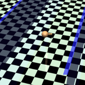
(a) Circle

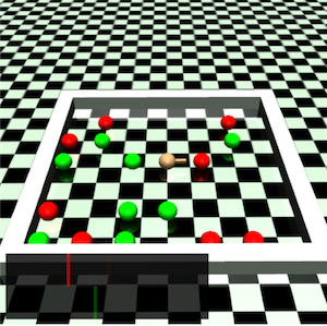
(b) Gather

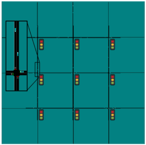
(c) Grid

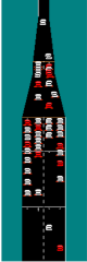
(d) Bottleneck

Figure 3: The Circle, Gather, Grid, and Bottleneck tasks. (a) Circle: The agent is rewarded for moving in a specified circle but is penalized if the diameter of the circle is larger than some value [3]. (b) Gather: The agent is rewarded for collecting the green balls while penalized to gather red balls [3]. (c) Grid: The agent controls traffic lights in a 3x3 road network and is rewarded for high traffic throughput but is constrained to let lights be red for at most 5 consecutive seconds [35]. (d) Botteneck: The agent controls vehicles (red) in a merging traffic situation and is rewarded for maximizing the number of vehicles that pass through but is constrained to ensure that white vehicles (not controlled by agent) have “low” speed for no more than 10 seconds. [35].

A.6.2 Learning Curves

Due to space restrictions, we present the learning curves for the remaining environments in Figure 4.

Average Rewards:

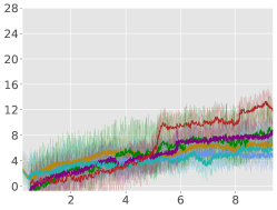
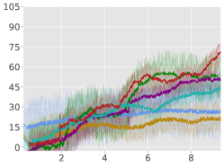
                    Average Constraint values:                       

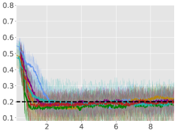
(a) Point Gather

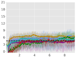
(b) Ant Circle

Figure 4: The average reward and constraint cost function values vs iterations (in $10^{4}$) learning curves for some algorithm-task pairs. Solid lines in each figure are the empirical means, while the shaded area represents 1 standard deviation, all over 5 runs. The dashed line in constraint plots is the constraint threshold $l$. ATRPO and PPO are tested with constraints, which are included in their Lagrangian formulation.

A.6.3 Recovery Regime Revisited

In Subsection 5.3, we studied the effect of the hyperparameter $t$ for only one task. Figure 5 shows the performance of ACPO with different values of $t$ in various environments.

Rewards:

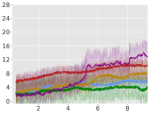
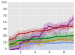
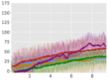
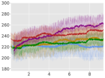
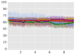
                    Constraint values:                                    

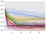
(a) Point Gather

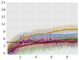
(b) Ant Circle

(c) Ant Gather

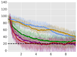
(d) Bottleneck

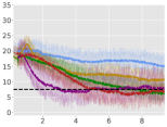
(e) Grid

Figure 5: Comparison of performance of ACPO with different values of the hyperparameter $t$ in various environment. X-axis is iterations in $10^{4}$.

References

• [1] J.Β Abounadi, D.Β Bertsekas, and V.Β S. Borkar. Learning algorithms for markov decision processes with average cost. SIAM Journal on Control and Optimization, 40(3):681–698, 2001.
• [2] J.Β Achiam. UC Berkeley CS 285 (Fall 2017), Advanced Policy Gradients, 2017. URL: http://rail.eecs.berkeley.edu/deeprlcourse-fa17/f17docs/lecture_13_advanced_pg.pdf. Last visited on 2020/05/24.
• [3] J.Β Achiam, D.Β Held, A.Β Tamar, and P.Β Abbeel. Constrained policy optimization. In Proceedings of the 34th International Conference on Machine Learning-Volume 70, pages 22–31. JMLR. org, 2017.
• [4] A.Β Agnihotri, P.Β Saraf, and K.Β R. Bapnad. A convolutional neural network approach towards self-driving cars. In 2019 IEEE 16th India Council International Conference (INDICON), pages 1–4, 2019.
• [5] M.Β Andrychowicz, A.Β Raichuk, P.Β StaΕ„czyk, M.Β Orsini, S.Β Girgin, R.Β Marinier, L.Β Hussenot, M.Β Geist, O.Β Pietquin, M.Β Michalski, etΒ al. What matters in on-policy reinforcement learning? a large-scale empirical study. arXiv preprint arXiv:2006.05990, 2020.
• [6] L.Β Chen, R.Β Jain, and H.Β Luo. Learning infinite-horizon average-reward Markov decision process with constraints. In K.Β Chaudhuri, S.Β Jegelka, L.Β Song, C.Β Szepesvari, G.Β Niu, and S.Β Sabato, editors, Proceedings of the 39th International Conference on Machine Learning, volume 162 of Proceedings of Machine Learning Research, pages 3246–3270. PMLR, 17–23 Jul 2022.
• [7] G.Β E. Cho and C.Β D. Meyer. Comparison of perturbation bounds for the stationary distribution of a markov chain. Linear Algebra and its Applications, 335(1-3):137–150, 2001.
• [8] P.Β G. Doyle. The kemeny constant of a markov chain. arXiv preprint arXiv:0909.2636, 2009.
• [9] Y.Β Gao, H.Β Xu, J.Β Lin, F.Β Yu, S.Β Levine, and T.Β Darrell. Reinforcement learning from imperfect demonstrations. arXiv preprint arXiv:1802.05313, 2018.
• [10] J.Β Garcia and F.Β Fernandez. A comprehensive survey on safe reinforcement learning. Journal of Machine Learning Research, 16(1):1437–1480, 2015.
• [11] C.Β M. Grinstead and J.Β L. Snell. Introduction to probability. American Mathematical Soc., 2012.
• [12] M.Β Haviv. On constrained markov decision processes. Operations research letters, 19(1):25–28, 1996.
• [13] H.Β Hu, Z.Β Liu, S.Β Chitlangia, A.Β Agnihotri, and D.Β Zhao. Investigating the impact of multi-lidar placement on object detection for autonomous driving. In Proceedings of the IEEE/CVF Conference on Computer Vision and Pattern Recognition (CVPR), pages 2550–2559, June 2022.
• [14] J.Β J. Hunter. Stationary distributions and mean first passage times of perturbed markov chains. Linear Algebra and its Applications, 410:217–243, 2005.
• [15] J.Β J. Hunter. Mathematical techniques of applied probability: Discrete time models: Basic theory, volumeΒ 1. Academic Press, 2014.
• [16] J.Β J. Hunter. The computation of the mean first passage times for markov chains. Linear Algebra and its Applications, 549:100–122, 2018.
• [17] N.Β Jiang, S.Β P. Singh, and A.Β Tewari. On structural properties of mdps that bound loss due to shallow planning. In IJCAI, pages 1640–1647, 2016.
• [18] S.Β Kakade and J.Β Langford. Approximately optimal approximate reinforcement learning. In International Conference on Machine Learning, volumeΒ 2, pages 267–274, 2002.
• [19] J.Β Kemeny and I.Β Snell. Finite Markov Chains. Van Nostrand, New Jersey, 1960.
• [20] L.Β Lehnert, R.Β Laroche, and H.Β van Seijen. On value function representation of long horizon problems. In Proceedings of the AAAI Conference on Artificial Intelligence, volumeΒ 32, 2018.
• [21] M.Β Levene and G.Β Loizou. Kemeny’s constant and the random surfer. The American mathematical monthly, 109(8):741–745, 2002.
• [22] S.Β Levine, C.Β Finn, T.Β Darrell, and P.Β Abbeel. End-to-end training of deep visuomotor policies. Journal of Machine Learning Research, 17(1):1334–1373, 2016.
• [23] P.Β Liao, Z.Β Qi, R.Β Wan, P.Β Klasnja, and S.Β A. Murphy. Batch policy learning in average reward markov decision processes. The Annals of Statistics, 50(6):3364–3387, 2022.
• [24] X.Β Ma, X.Β Tang, L.Β Xia, J.Β Yang, and Q.Β Zhao. Average-reward reinforcement learning with trust region methods. arXiv preprint arXiv:2106.03442, 2021.
• [25] A.Β Rajeswaran, V.Β Kumar, A.Β Gupta, G.Β Vezzani, J.Β Schulman, E.Β Todorov, and S.Β Levine. Learning complex dexterous manipulation with deep reinforcement learning and demonstrations. arXiv preprint arXiv:1709.10087, 2017.
• [26] H.Β Satija, P.Β Amortila, and J.Β Pineau. Constrained Markov decision processes via backward value functions. In H.Β D. III and A.Β Singh, editors, Proceedings of the 37th International Conference on Machine Learning, volume 119 of Proceedings of Machine Learning Research, pages 8502–8511. PMLR, 13–18 Jul 2020.
• [27] J.Β Schulman, S.Β Levine, P.Β Abbeel, M.Β Jordan, and P.Β Moritz. Trust region policy optimization. In International Conference on Machine Learning, pages 1889–1897, 2015.
• [28] J.Β Schulman, P.Β Moritz, S.Β Levine, M.Β Jordan, and P.Β Abbeel. High-dimensional continuous control using generalized advantage estimation. International Conference on Learning Representations (ICLR), 2016.
• [29] J.Β Schulman, F.Β Wolski, P.Β Dhariwal, A.Β Radford, and O.Β Klimov. Proximal policy optimization algorithms. arXiv preprint arXiv:1707.06347, 2017.
• [30] D.Β Silver, J.Β Schrittwieser, K.Β Simonyan, I.Β Antonoglou, A.Β Huang, A.Β Guez, T.Β Hubert, L.Β Baker, M.Β Lai, A.Β Bolton, etΒ al. Mastering the game of go without human knowledge. nature, 550(7676):354–359, 2017.
• [31] H.Β F. Song, A.Β Abdolmaleki, J.Β T. Springenberg, A.Β Clark, H.Β Soyer, J.Β W. Rae, S.Β Noury, A.Β Ahuja, S.Β Liu, D.Β Tirumala, etΒ al. V-mpo: on-policy maximum a posteriori policy optimization for discrete and continuous control. International Conference on Learning Representations, 2020.
• [32] C.Β Tessler, D.Β J. Mankowitz, and S.Β Mannor. Reward constrained policy optimization. International Conference on Learning Representation (ICLR), 2019.
• [33] R.Β J. Tibshirani. Dykstra’s algorithm, admm, and coordinate descent: Connections, insights, and extensions. Advances in Neural Information Processing Systems, 30, 2017.
• [34] E.Β Todorov, T.Β Erez, and Y.Β Tassa. Mujoco: A physics engine for model-based control. In 2012 IEEE/RSJ International Conference on Intelligent Robots and Systems, pages 5026–5033. IEEE, 2012.
• [35] E.Β Vinitsky, A.Β Kreidieh, L.Β LeΒ Flem, N.Β Kheterpal, K.Β Jang, F.Β Wu, R.Β Liaw, E.Β Liang, and A.Β M. Bayen. Benchmarks for reinforcement learning in mixed-autonomy traffic. In Proceedings of Conference on Robot Learning, pages 399–409, 2018.
• [36] O.Β Vinyals, I.Β Babuschkin, W.Β M. Czarnecki, M.Β Mathieu, A.Β Dudzik, J.Β Chung, D.Β H. Choi, R.Β Powell, T.Β Ewalds, P.Β Georgiev, etΒ al. Grandmaster level in starcraft ii using multi-agent reinforcement learning. Nature, 575(7782):350–354, 2019.
• [37] Q.Β Vuong, Y.Β Zhang, and K.Β W. Ross. Supervised policy update for deep reinforcement learning. In International Conference on Learning Representation (ICLR), 2019.
• [38] Y.Β Wan, A.Β Naik, and R.Β S. Sutton. Learning and planning in average-reward markov decision processes. In International Conference on Machine Learning, pages 10653–10662. PMLR, 2021.
• [39] C.-Y. Wei, M.Β J. Jahromi, H.Β Luo, and R.Β Jain. Learning infinite-horizon average-reward mdps with linear function approximation. In International Conference on Artificial Intelligence and Statistics, pages 3007–3015. PMLR, 2021.
• [40] L.Β Wen, J.Β Duan, S.Β E. Li, S.Β Xu, and H.Β Peng. Safe reinforcement learning for autonomous vehicles through parallel constrained policy optimization. In 2020 IEEE 23rd International Conference on Intelligent Transportation Systems (ITSC), pages 1–7. IEEE, 2020.
• [41] Y.Β Wu, E.Β Mansimov, R.Β B. Grosse, S.Β Liao, and J.Β Ba. Scalable trust-region method for deep reinforcement learning using kronecker-factored approximation. In Advances in neural information processing systems (NIPS), pages 5285–5294, 2017.
• [42] T.-Y. Yang, J.Β Rosca, K.Β Narasimhan, and P.Β J. Ramadge. Projection-based constrained policy optimization. In International Conference on Learning Representation (ICLR), 2020.
• [43] S.Β Zhang, Y.Β Wan, R.Β S. Sutton, and S.Β Whiteson. Average-reward off-policy policy evaluation with function approximation. arXiv preprint arXiv:2101.02808, 2021.
• [44] Y.Β Zhang and K.Β Ross. Average reward reinforcement learning with monotonic policy improvement. Preprint, 2020.