Unsupervised Entity Alignment for Temporal Knowledge Graphs

Abstract.

Entity alignment (EA) is a fundamental data integration task that identifies equivalent entities between different knowledge graphs (KGs). Temporal Knowledge graphs (TKGs) extend traditional knowledge graphs by introducing timestamps, which have received increasing attention. State-of-the-art time-aware EA studies have suggested that the temporal information of TKGs facilitates the performance of EA. However, existing studies have not thoroughly exploited the advantages of temporal information in TKGs. Also, they perform EA by pre-aligning entity pairs, which can be labor-intensive and thus inefficient. In this paper, we present DualMatch that effectively fuses the relational and temporal information for EA. DualMatch transfers EA on TKGs into a weighted graph matching problem. More specifically, DualMatch is equipped with an unsupervised method, which achieves EA without necessitating the seed alignment. DualMatch has two steps: (i) encoding temporal and relational information into embeddings separately using a novel label-free encoder, Dual-Encoder; and (ii) fusing both information and transforming it into alignment using a novel graph-matching-based decoder, GM-Decoder. DualMatch is able to perform EA on TKGs with or without supervision, due to its capability of effectively capturing temporal information. Extensive experiments on three real-world TKG datasets offer the insight that DualMatch significantly outperforms the state-of-the-art methods.

1. Introduction

Knowledge graphs (KGs) represent structured knowledge related to real-world objects, which plays a crucial role in many real-world applications, such as semantic search (Xiong et al., 2017), entity (Zhang et al., 2021, 2022; Jiang et al., 2022b, a) and relation extraction (Hu et al., 2021a; Liu et al., 2022a; Hu et al., 2021b, 2020). However, existing KGs are generally highly incomplete (Sun et al., 2020c). Since different KGs are constructed from various data sources, they contain unique information but have overlapped entities. This scenario provides us an opportunity to integrate different KGs with the overlapped entities.

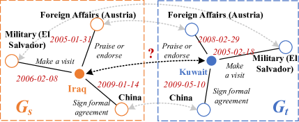
Figure 1. An example of limitations of existing methods without considering temporal information

A typical strategy for integration of KGs is Entity Alignment (EA) (Sun et al., 2020c), which aligns entities from different KGs that refer to the same real-world objects. Given two KGs and a small set of pre-aligned entities (also known as seed alignment), EA identifies all possible alignments between them. Existing embedding-based studies (Li et al., 2019; Mao et al., 2020b; Sun et al., 2020b, a; Mao et al., 2021a) have proven highly effective to perform EA, which is mainly benefited by the use of Graph Neural Networks (GNNs) (Kipf and Welling, 2017; Velickovic et al., 2018; Hamilton et al., 2017). They assume that the neighbors of two equivalent entities in separated KGs are also equivalent (Liu et al., 2020). Based on this assumption, they align entities by applying representation learning to KGs. We summarize the process of Embedding-based EA as the following two steps: (i) encoding entities of two KGs into embedding vectors by training an EA model with some seed alignments; and (ii) decoding the embedding vectors of the entities into an alignment matrix, based on a specific similarity measurement (e.g., cosine similarity) of their embeddings.

Most of the existing EA studies need to pre-align training sets before an embedding model can be trained, which is labor-intensive and degrades their usability in real-world applications (Sun et al., 2020c). These problems can be tackled by name-based (Liu et al., 2020; Ge et al., 2022; Zeng et al., 2020; Mao et al., 2021b; Ge et al., 2021a; Wang et al., 2022; Ge et al., 2021b) or image-based (Liu et al., 2021) models via incorporating side information, where few or no label is required for performing EA. However, such models still suffer from problems. First, the performance of the name-based models is overestimated due to name-bias (Chen et al., 2021; Liu et al., 2020, 2021; Sun et al., 2021). In this case, the ground truths (inter graph/language links) are generally generated with the entity name, and thus results in test data leakage when they are served as features. Second, the images are not inherent parts of KGs and are thus hard to be collected. As a result, incorporating side information may not be able to enhance EA. Moreover, most of the existing EA methods (Chen et al., 2017; Cao et al., 2019; Chen et al., 2021; Mao et al., 2020a, b, 2021b, 2021a; Li et al., 2019; Liu et al., 2021, 2020; Mao et al., 2022) do not consider temporal information. This results in incorrect predictions on entities, which have similar neighborhood structures in relational triples but correspond to different time intervals, as shown in Figure 1.

Temporal information are often utilized to enhance the performance of various applications (Li et al., 2020, 2021). Temporal Knowledge Graphs (TKGs) (Suchanek et al., 2007; Vrandecic and Krötzsch, 2014), a type of KGs, have been proposed that associates relational facts with temporal information. As the formats of storing temporal information in TKGs are almost identical, the alignment information can be obtained easily, which naturally enhances the EA performance. Nevertheless, recent studies (Xu et al., 2021, 2022) that applies TKGs to EA still suffer from the following two problems.

• “Redundantly” pre-aligned seeds. They (Xu et al., 2021, 2022) follow studies that applies KGs to EA, which cannot perform EA until the pre-aligned seeds are obtained. However, unlike KGs, temporal information in relational triples of TKGs is naturally aligned since they represent real-world time points or time periods (Xu et al., 2021, 2022). This character of TKGs provides the opportunity of developing time-aware EA methods in an unsupervised fashion by treating temporal information as seed alignment.

• Insufficient temporal information discovery. They (Xu et al., 2021, 2022) simply create embeddings for each timestamp, and treat the time intervals as relation types to enhance the graph learning process. These processes highly rely on the seed alignment, where the temporal information has not been fully exploited, and thus the accuracy of EA is limited. We use an example to illustrate it.

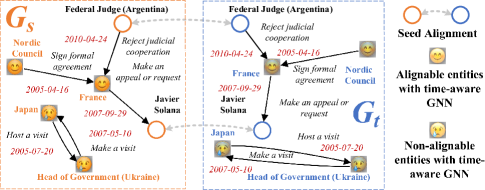
Figure 2. A corner case of possible misalignment for previous time-aware GNN studies

Example 1.1.

Assume that we have trained an accurate time-aware GNN on these graphs that could maximally propagate all the alignment information, as depicted in Figure 2. In this case, the entity “Japan” is likely to be misaligned due to two reasons: (1) “Japan” and the seeds are in different connected components, where the GNNs is unlikely to propagate the alignment information to the embedding of “Japan”; and (2) “Japan” does not share common timestamps and relation types with the seeds, and thus, the information of seeds is unable to reach “Japan” via shared temporal or relational embeddings. This misalignment of Japan renders it is excluded from the objective of the learned model. However, as shown in Figure 2, each entity has at least one outgoing edge with a unique timestamp. As a result, following the 1-to-1 mapping assumption (Chen et al., 2017), “Japan” can be aligned correctly, by simply hashing the entities using the timestamps of their outgoing edge.

We present an EA method for TKGs, DualMatch, that is able to address the above two problems. To tackle the first problem, instead of treating time intervals simply as relations (Xu et al., 2021, 2022), we model the temporal information using a learning-free encoder. Specifically, we derive pseudo seeds from the encoder to train GNN-based EA models. The models can encode relational information without any requirement for training data. To solve the second problem, we develop a decoder that is independent of seed alignment. This is to fuse the temporal and relational information after they are encoded into feature vectors. We transform EA into weighted graph matching, in order to wisely balance the temporal and relational information. Our contributions are summarized as follows:

• Framework. We design DualMatch , an EA framework for TKGs, which effectively explores both temporal and relational information. It contains two steps: (i) encoding the information from TKGs, and (ii) decoding the embedded data into an alignment matrix. By employing an encoder Dual-Encoder and a decoder GM-Decoder, DualMatch can perform EA on TKGs with or without training data.

• Encoder. We develop a novel Dual-Encoder that encodes the temporal and relational information separately. Dual-Encoder has two components: (i) Temporal-Encoder that retains the temporal information in TKGs; and (ii) Relational-Encoder that learns the relational information using the graph structure.

• Decoder. We design a novel GM-Decoder that balances the graph structure information and temporal information wisely, by building a bridge between the EA task and the weighted graph matching task.

• Experiments. We conduct comprehensive experiments on three real-world datasets, which suggest that DualMatch is able to outperform existing TKG models (Xu et al., 2021, 2022) in terms of accuracy in both supervised and unsupervised settings.

2. Related Work

Entity Alignment Encoders. Most existing EA encoders are designed to learn the graph structures of KGs. They can be divided into two categories: KGE-based Encoder (Chen et al., 2017; Zhu et al., 2017; Sun et al., 2018; Trisedya et al., 2019) and GNN-based Encoder (Wang et al., 2018; Li et al., 2019; Mao et al., 2020a; Sun et al., 2020b, a; Cao et al., 2019; Mao et al., 2021a). The former uses the KG embedding models (e.g., TransE (Bordes et al., 2013)) to learn entity embeddings, while the latter uses GNNs (Kipf and Welling, 2017). Recently, GNN-based models have demonstrated their outstanding performance (Mao et al., 2021a). This is contributed by the strong modeling capability of GNNs to capture graph structure with anisotropic attention mechanism (Velickovic et al., 2018). However, they are not capable of modeling temporal information in TKGs.

Temporal EA Encoders. TEA-GNN (Xu et al., 2021) and TREA (Xu et al., 2022) incorporate temporal information into the GNN architecture with timestamp. However, these methods have not fully explored the underlying efficacy of temporal information in GNN encoder embeddings and require seed alignment for EA. On the contrary, the proposed Dual-Encoder processes the temporal and relational information separately to improve the performance and is able to perform without seed alignment.

Entity Alignment Decoders. Most existing EA decoders are designed to find equivalent entities based on the learned embeddings. The most commonly used decoder is greedy search (Sun et al., 2020c). It essentially finds the top-1-nearest neighbor using the similarity between embeddings of entities (Chen et al., 2017; Zhu et al., 2017; Sun et al., 2018, 2020c). To enhance the performance of EA, CSLS (Lample et al., 2018) proposes to normalize the similarity matrix. However, the performance of CSLS’ greedy top-1-nearest neighbor search is limited because it can only partly normalize the similarity matrix using local nearest neighbors. CEA (Zeng et al., 2020) adopts the Deferred-acceptance algorithm (DAA) (Roth, 2008) to find the stable matching between entities of two KGs, which produces higher-quality results than CSLS. Nonetheless, DAA is hard to be parallelized on GPU as it performs iterations to match and un-match entity pairs. SEU (Mao et al., 2021b) transforms EA into the assignment problem by employing Hungarian algorithm (Harold W. Kuhn, 1955) or Sinkhorn algorithm (Cuturi, 2013) to normalize the similarity matrix. DATTI (Mao et al., 2022) decodes embeddings using Third-order Tensor Isomorphism. Recent studies  (Ge et al., 2022; Gao et al., 2022; Zeng et al., 2022; Liu et al., 2022b; Xin et al., 2022) also present several decoders that exploit sampling to process large-scale EA. Different from previous decoders, our proposed GM-Decoder is designed for decoding features of TKGs. It needs two sets of input features, and effectively fuses them to generate high-quality alignment.

Unsupervised EA. All existing proposals of unsupervised EA employ side information of KGs, including literal information of entity names (Ge et al., 2021a; Mao et al., 2021b) and visual information (Liu et al., 2021). Such proposals are able to perform EA without seed alignment  (Sun et al., 2020c). However, models that incorporate machine translation or pre-aligned word embeddings may be overestimated due to the name bias issue (Chen et al., 2021; Liu et al., 2020, 2021; Sun et al., 2021). In addition, it is difficult to extract visual information from KGs. On the contrary, our presented DualMatch only requires the information that is easily obtained from the TKGs in this paper and does not suffer from the name bias issue.

3. Preliminaries

We proceed to introduce preliminary definitions. Based on these, we formalize the problem of time-aware entity alignment.

3.1. Assignment Problem

Assignment problem is a well-established combinatorial optimization problem. It aims to find the optimal assignment $\bm{P}$ that transfers from a source distribution to a target distribution, while maximizing the overall profit. Finding optimal $\bm{P}$ can be viewed as a special case of the optimal transport problem (Mena et al., 2018). In this paper, we adopt the Sinkhorn algorithm (Cuturi, 2013) to solve the assignment problem, which iterates $k$ steps for scaling the similarity/cost matrix.

An extension of the assignment problem is the quadratic assignment problem, which extends the assignment problem by defining the profit function in terms of quadratic inequalities. It is also commonly known as the weighted graph matching problem (Gold and Rangarajan, 1996). Given two adjacency matrices $\bm{K_{X}}\in\mathbb{R}^{N\times N}$ and $\bm{K_{Y}}\in\mathbb{R}^{N\times N}$, the weighted graph matching problem aims to find an optimal $\bm{P}\in\mathbb{P}_{N}$ such that $\|\bm{K_{X}}\bm{P}-\bm{P}\bm{K_{Y}}\|_{2}^{2}$ is minimized.

3.2. Graph Kernel

A graph kernel is a kernel function widely used in structure mining, which computes an inner product on graphs. Graph kernels can be used to compute how similar two graphs are. Thus, we use Weisfeiler-Lehman (WL) Subtree Kernel (Shervashidze et al., 2011), one of the most commonly-used graph kernels, to detect the similarity between two adjacency matrices. It calculates the similarity of graphs by running the WL Isomorphism Test (Weisfeiler and Leman, 1968). Specifically, given a set $\mathcal{S}_{G}$ of graphs, we compute the WL kernel matrix $K_{WL}^{(h)}\in\mathbb{R}^{|\mathcal{S}_{G}|\times|\mathcal{S}_{G}|}$. For each pair of graphs $(G_{i},G_{j})\in\mathcal{S}_{G}\times\mathcal{S}_{G}$, we have

(1) $$k_{WL}^{(h)}(G_{i},G_{j})=\sum_{k=0}^{h}\left\langle\phi\left(G_{i}^{(k)}\right),\phi\left(G_{j}^{(k)}\right)\right\rangle$$

where $h$ is the number of WL iterations, $\left\{G^{(0)},\ldots,G^{(h)}\right\}$ are the WL sequences of one graph $G$, and $\phi\left(G\right)$ indicates the feature mapping obtained from The WL Isomorphism Test. A traditional strategy to normalize the kernel matrix is to divide it by its diagonal, in which each element represents the similarity of a graph with itself, i.e., $\hat{k}_{WL}(G_{i},G_{j})=\frac{k_{WL}(G_{i},G_{j})}{\sqrt{diag(\bm{K}_{WL})\otimes diag(\bm{K}_{WL})}}.$

3.3. Problem Definitions

Definition 1.

A temporal knowledge graph (TKG) can be denoted as $G=(E,R,T,Q)$, where $E$ is the set of entities, $R$ is the set of relations, $T$ is the set of time intervals, and $Q=\{(h,r,t,\tau)~{}|~{}h,t\in E,r\in R,\tau\in T\}$ is the set of quadruples, each of which represents that the subject entity $h$ has the relation $r$ with the object entity $t$ during the time interval $\tau$. $\tau$ is represented as $[t_{b},t_{e}]$, with the beginning timestamp $t_{b}$ and the ending timestamp $t_{e}$. Some of the event-style quadruples, e.g., quadruples with the relation type “born-in”, may have $t_{b}=t_{e}$.

Definition 2.

Time-aware Entity alignment (TEA) (Xu et al., 2021) aims to find a 1-to-1 mapping of entities $\phi$ from a source TKG $G_{s}=(E_{s},R_{s},T^{*},Q_{s})$ to a target TKG $G_{t}=(E_{t},R_{t},T^{*},Q_{t})$, where $T^{*}$ is a set of time intervals overlapped between $G_{s}$ and $G_{t}$. $\phi=\{(e_{s},e_{t})\in E_{s}\times E_{t}~{}|~{}e_{s}\equiv e_{t}\}$ , where $e_{s}\in E_{s}$, $e_{t}\in E_{t}$, and $\equiv$ is an equivalence relation between two entities.

In supervised settings, a small set of equivalent entities $\phi^{\prime}\subset\phi$ is known beforehand, and is used as seed alignment. In unsupervised settings, the seed alignment $\phi^{\prime}$ is unknown.

4. Methodology

We present our framework DualMatch for TKGs. We start by giving the overview of DualMatch and then detail each component of it.

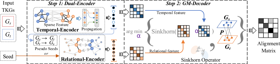
Figure 3. DualMatch framework

4.1. Overview

Figure 3 shows DualMatch framework. The input (left side of Figure  3) includes two TKGs $G_{s}$,$G_{t}$, and an optional slot for seed alignment. In order to transfer the temporal and relational information of TKGs into a better alignment result, DualMatch employs a Dual-Encoder (cf Step 1 of Figure 3). It has two components to encode the input TKGs: (i) Temporal-Encoder that aims at retaining the temporal information in TKGs; and (ii) Relational-Encoder that aims at learning the relational information using the graph structure. With Dual-Encoder, the temporal and relational information are encoded into separate entity features. Next, DualMatch develops GM-Decoder (cf Step 1 of Figure 3), which effectively fuses the temporal features with relational features by transforming the EA task into the weighted graph matching task. After the transformation, the GM-Decoder can produce a near-optimal fused alignment matrix (right side of Figure 3). Algorithm 1 depicts the pseudo-code of the DualMatch framework.

4.2. Encoding Temporal Information

Since the two TKGs to be aligned share the same set of time intervals that are recorded in quadruples, it is reasonable to make the following assumption: if two entities $e_{s}\in E_{s}$ and $e_{t}\in E_{t}$ have many overlapped time intervals between their connected quadruples, $e_{s}$ and $e_{t}$ are very likely to represent the same real-world object. Based on this assumption, we propose a simple yet effective Temporal-Encoder. Temporal-Encoder builds temporal features for entities in TKGs using their overlapped time intervals. For a TKG, we extract a bipartite graph $A^{t}$ between $E$ and $T$. For each $a^{t}_{et}\in A^{t}$, we have

(2) $$a^{t}_{et}=\frac{\text{exp}(|Q_{et}|)}{\sum_{\tau\in T}\text{exp}(|Q_{e\tau}|)},$$

where $|Q_{et}|$ is the number of quadruples that contain both entity $e$ and time interval $t$. Here, we separately calculate and concatenate the temporal adjacency matrices for head entities and tail entities. Thus, the result dimension of $A^{t}$ is $\left|E\right|\times\left|2T\right|$. We call this bipartite graph the temporal feature matrix of $E$.

With the temporal feature matrices, $\bm{A}^{t}_{s}$ of $G_{s}$ and $\bm{A}^{t}_{t}$ of $G_{t}$, an alignment matrix can be easily derived by calculating the pairwise similarity: $\bm{P}=\bm{A}^{t}_{s}(\bm{A}^{t}_{t})^{T}$. However, some entities may not contain sufficient temporal information, which leads to poor alignment results. To solve this problem, we impute the temporal feature from their neighborhoods, which may have a link to sufficient temporal facts, by aggregating information from neighbors; thus follow (Mao et al., 2021b) to perform a $L$-layers graph-convolution-like forward pass to obtain an aggregated feature matrix: $\bm{H}^{t}=\left[\bm{A^{t}}||\bm{A}\bm{A^{t}}||\bm{A}^{2}\bm{A^{t}}||...||\bm{A}^{L}\bm{A^{t}}\right]$ (cf. Lines 3-4 of Algorithm 1), where $L$ is a hyper-parameter indicating number of layers of the graph-convolution-like forward pass, $[X||Y]$ indicates tensor concatenate operations between $X$ and $Y$ along the last dimension, and $\bm{A}^{l}=\prod_{i\in 1,...,l}\bm{A}$ is the $l$-hop adjacency matrix of $G$. Here, to leverage the impact of different relation types on the knowledge graph, we follow (Mao et al., 2020a, b, 2021a, 2021b, 2022) to build the relational feature matrix. Specifically, for each $\bm{a}_{ij}\in\bm{A}$ ,

(3) $$\bm{a}_{ij}=\frac{\sum_{r_{j}\in R_{i,j}}\ln\left(|Q|/\left|Q_{r_{j}}\right|\right)}{\sum_{k\in\mathcal{N}_{i}}\sum_{r_{k}\in R_{i,k}}\ln\left(|Q|/\left|Q_{r_{k}}\right|\right)},$$

where $\mathcal{N}_{i}$ represents the neighboring set of entity $e_{i},R_{i,j}$ is the relation set between $e_{i}$ and $e_{j}$, and $|Q|$ and $\left|Q_{r}\right|$ denote the total number of all quadruples and the quadruples containing relation $r$, respectively.

4.3. Encoding Relational Information

State-of-the-art methods for encoding relational information typically use GNNs (Kipf and Welling, 2017) to propagate the information provided by the seed alignment $\phi^{\prime}$. Studies (Xu et al., 2021, 2022) suggest that integrating temporal information can improve the performance of EA. They encode entities’ relational features together with temporal features using a GNN. Specifically, they train the entity’s embedding by propagating the neighborhood information (Mao et al., 2020b; Kipf and Welling, 2017; Velickovic et al., 2018). The embedding of an entity $v\in E$ in the $l^{th}$ layer of GNN $h_{v}^{(l)}$ is computed by aggregating localized information:

(4) $$\begin{array}[]{c}a_{v}^{(l)}=\operatorname{AGGREGATE}^{(l)}\left(\left\{\left(h_{u}^{(l-1)},\textbf{r}_{uv},\textbf{t}_{uv}\right)\mid u\in\mathcal{N}(v)\right\}\right)\\ h_{v}^{(l)}=\operatorname{UPDATE}^{(l)}\left(a_{v}^{(l)},h_{v}^{(l-1)}\right),\end{array}\vspace{-2mm}$$

where $h_{v}^{0}\in\mathbb{R}^{D}$ is a learnable embedding vector initialized using Glorot initialization, $\textbf{r}_{uv}\in R$, $\textbf{t}_{uv}\in T$ represents the relation types and time intervals between entity $u$ and $v$, and $\mathcal{N}(v)$ is the set of neighboring entities around $v$. The model’s final output is denoted as $\bm{H}^{r}\in\mathbb{R}^{|E_{s}\cup E_{t}|\times D}$, where $D$ is the dimension of embeddings.

Relational-Encoder adopts the state-of-the-art EA method (Mao et al., 2021a) to build a $L$-layer GNN model for learning the representation of the knowledge graph structure (cf. Line 9 of Algorithm 1). To be more specific, the dual-aspect embedding in (Mao et al., 2021a) concatenates both entity embeddings and relation embeddings. We extend it with additional time embeddings to form an overall triple-aspect embedding. For each $\bm{h}_{e_{i}}\in\bm{H}^{r}$:

(5) $$\bm{h}_{e_{i}}=\left[\bm{h}_{e_{i}}^{out}\|\left(\frac{1}{\left|\mathcal{N}_{e_{i}}^{r}\right|}\sum_{r_{j}\in\mathcal{N}_{e_{i}}^{r}}\bm{h}_{r_{j}}+\frac{1}{\left|\mathcal{N}_{e_{i}}^{t}\right|}\sum_{t_{j}\in\mathcal{N}_{e_{i}}^{t}}\bm{h}_{t_{j}}\right)\right],$$

where $\bm{h}_{e_{i}}^{out}=[h_{e_{i}}^{(0)}||h_{e_{i}}^{(1)}||...||h_{e_{i}}^{(L)}],\bm{h}_{r_{j}}$, and $\bm{h}_{t_{j}}$ denote the vector of corresponding entity, relation, and time interval respectively, and $\mathcal{N}_{e_{i}}^{r}$ and $\mathcal{N}_{e_{i}}^{t}$ represent the set of the relations and time intervals around entity $e_{i}$. Note that recent works generally concatenate all the output features in each GNN layer (Mao et al., 2020a, b, 2021a), in order to achieve better performance. Previous studies use negative sampling (Chen et al., 2017; Liu et al., 2020; Mao et al., 2020a) to form the loss function and to train the encoder model. We adopt this strategy for fast convergence (Mao et al., 2021a; Xu et al., 2022). The training loss is defined as $\mathcal{L}=\text{LSE}(\lambda z(e_{s},e_{t}))+\text{LSE}(\lambda z(e_{t},e_{s}))$ , where $e_{s}\in E_{s}$, $e_{t}\in E_{t}$, $(e_{s},e_{t})\in\phi^{\prime}$, $\text{LSE}(X)=log(\sum_{x\in X}e^{x})$ is an operator to smoothly generates hard negative samples, $\lambda$ is the smooth factor of LSE, and $z\in\mathcal{R}^{|E_{t}|}$ is the normalized triple loss. More specifically, $z$ is defined as $z(e_{s},e_{t})=\operatorname{z-score}(\{\gamma+\operatorname{sim}(e_{s},e_{t})-\operatorname{sim}(e_{s},e_{t}^{\prime})|e^{\prime}_{t}\in E_{t}\}),$ in which $\operatorname{z-score}(X)=\frac{X-\mu(X)}{\sigma(X)}$ is the standard score normalization, and $\operatorname{sim}(e_{s},e_{t})=\bm{h}^{r}_{e_{s}}\cdot\bm{h}^{r}_{e_{t}}$ is the similarity of two entities obtained by the dot product.

4.4. Fusing Information and Decoding

Naive Strategy

Previous studies have developed several techniques to improve EA performance by decoding embeddings into an alignment matrix. However, in GM-Decoder, the temporal and relational information is separately encoded into $\bm{H}^{t}$ and $\bm{H}^{r}$. A naive strategy is to directly concatenate two features by $\bm{\hat{H}}=\left[\bm{H}^{r}||\bm{H}^{t}\right]$. and then we can obtain the alignment matrix according to the concatenated features: $\bm{P}=\bm{\hat{H}}_{s}(\bm{\hat{H}}_{t})^{T}.$

Our Strategy

The naive decoding strategy has two problems. First, $\bm{H}^{r}$ is a dense matrix while $\bm{H}^{t}$ is sparse in practice. Due to the commonly used format of storing sparse matrices, it is memory-consuming to concatenate one sparse matrix with a dense matrix. Second, $\bm{H}^{r}$ is obtained from Relational-Encoder while $\bm{H}^{t}$ is obtained from Temporal-Encoder. Thus they are not required to be considered equally. To address the aforementioned two problems, we introduce a weight $\alpha$: $\bm{P}=\alpha\cdot\bm{H}^{t}_{s}(\bm{H}_{t}^{t})^{T}+\bm{H}^{r}_{s}(\bm{H}^{r}_{t})^{T}$, where $\alpha$ is the weight to balance the impact of the two features on the alignment result. Then, to normalize the alignment matrix, we adopt recent work (Mao et al., 2021b, 2022) that reformulated EA as an assignment problem and solved it via the Sinkhorn algorithm (Mao et al., 2021b; Ge et al., 2021a; Gao et al., 2022; Mao et al., 2022): $\bm{\hat{P}}=\text{Sinkhorn}\left(\bm{P}\right)$ (cf. Line 13 of Algorithm 1). Note that, $|E_{s}|\not\eq|E_{t}|$ in many real-world scenarios. In this case, the EA problem is transformed into an unbalanced assignment problem, which can then be straightforwardly reformulated as a balanced assignment problem (Mao et al., 2021b).

However, the optimal $\alpha$ is hard to be determined because the ground truth is unknown. To solve this problem, we study the isomorphic nature of the two TKGs to be aligned and propose to set the weight by minimizing the objective of weighted graph matching (Gold and Rangarajan, 1996) with given $\bm{\hat{P}}$. More specifically, we map the source adjacency matrices into target ones. Next, by calculating the distance of the mapped matrix with the target matrix, we derive the correctness of the alignment matrix $\bm{\hat{P}}$ (cf. Line 14 of Algorithm 1).

(6) $$\bm{D}_{G_{s}G_{t}}=k^{r}\left\|\bm{A}_{s}\bm{\hat{P}}-\bm{\hat{P}}\bm{A}_{t}\right\|_{2}^{2}+k^{t}\left\|\bm{A}_{s}^{t}-\bm{\hat{P}}\bm{A}_{t}^{t}\right\|_{2}^{2},$$

where $k^{r}=\hat{k}_{WL}(\bm{A_{s}},\bm{A_{t}})$ and $k^{t}=\hat{k}_{WL}(\bm{A_{s}^{t}},\bm{A_{t}^{t}})$ are the weights based on the isomorphism of the adjacency matrices.

Let $d^{r}=\left\|\bm{A}_{s}\bm{\hat{P}}-\bm{\hat{P}}\bm{A}_{t}\right\|_{2}^{2}$ and $d^{t}=\left\|\bm{A}_{s}^{t}-\bm{\hat{P}}\bm{A}_{t}^{t}\right\|_{2}^{2}$ be the distances of the two TKGs measured by the relational and temporal feature matrices. Since the two TKGs may be non-isomorphic, and the relational adjacency matrices and temporal adjacency matrices are constructed independently, $d^{r}$ and $d^{t}$ may scale differently. Hence, it is reasonable to assign different weights to them. We denote $sim(\cdot)$ as the similarity between two adjacency matrices. Intuitively, if we have $sim(\bm{A_{s}},\bm{A_{t}})>sim(\bm{A^{t}_{s}},\bm{A^{t}_{t}})$, $d^{r}$ can be weighted more. This motivates us to set the weights using the similarity of graphs measured by the WL Graph Kernels (Shervashidze et al., 2011).

Input: TKGs $G_{s}$, $G_{t}$, optional seed alignment $\phi^{\prime}$, and range $R_{\alpha}$

Output: Alignment matrix $\bm{\hat{P}}$

1

/* Step $1$: encode temporal and relational information into vectors with Dual-Encoder */

2 $\bm{A}_{s},\bm{A}^{t}_{s},\leftarrow G_{s}$, $\bm{A}_{t},\bm{A}^{t}_{t}\leftarrow G_{t}$ /* Extract feature matrices */

3 $\bm{H}^{t}_{s}\leftarrow$ Temporal-Encoder($\bm{A}_{s},\bm{A}^{t}_{s}$)

4 $\bm{H}^{t}_{t}\leftarrow$ Temporal-Encoder($\bm{A}_{t},\bm{A}^{t}_{t}$)

5 if $\phi^{\prime}$ is $not$ $given$ then /* Compute pseudo-seeds */

6       $\bm{P}^{G_{s}G_{t}}\leftarrow\text{Sinkhorn}(\bm{H}^{t}_{s}(\bm{H}^{t}_{t})^{T})$

7       $\bm{P}^{G_{t}G_{s}}\leftarrow\text{Sinkhorn}(\bm{H}^{t}_{t}(\bm{H}^{t}_{s})^{T})$

8       $\phi^{\prime}\leftarrow\{(i,j)|\arg\max_{j^{\prime}}{\bm{P}^{G_{s}G_{t}}_{ij^{\prime}}}=j\wedge\arg\max_{i^{\prime}}{\bm{P}^{G_{t}G_{s}}_{ji^{\prime}}}=i\}$

9

10$\bm{H}^{r}_{s},\bm{H}^{r}_{t}\leftarrow$ Relational-Encoder($G_{s},G_{t},\phi^{\prime}$)

/* Step $2$: decode feature vectors with GM-Decoder */

11 $\bm{\hat{P}},\bm{D}\leftarrow zeros(|E_{s}|,|E_{t}|),+\infty$

12 for $\alpha\in R_{\alpha}$ do

13       $\bm{\hat{P}}_{\alpha}\leftarrow\text{Sinkhorn}(\alpha\cdot\bm{H}^{t}_{s}(\bm{H}_{t}^{t})^{T}+\bm{H}^{r}_{s}(\bm{H}^{r}_{t})^{T})$

14       $\bm{D}_{G_{s}G_{t}}^{\alpha}=k^{r}\left\|\bm{A}_{s}\bm{\hat{P}}_{\alpha}-\bm{\hat{P}}_{\alpha}\bm{A}_{t}\right\|_{2}^{2}+k^{t}\left\|\bm{A}_{s}^{t}-\bm{\hat{P}}_{\alpha}\bm{A}_{t}^{t}\right\|_{2}^{2}$

15       if $\bm{D}_{G_{s}G_{t}}^{\alpha}<\bm{D}$ then

16             $\bm{D},\bm{\hat{P}}\leftarrow\bm{D}_{G_{s}G_{t}}^{\alpha},\bm{\hat{P}}_{\alpha}$/* Update alignment matrix */

17      

18

19return $\bm{\hat{P}}$.

Algorithm 1 The proposed DualMatch process

We search $\alpha=\arg\min_{\alpha}\bm{D}_{G_{s}G_{t}}$ in the range of $R_{\alpha}$, in order to obtain the optimal $\bm{\hat{P}}$ (cf. Lines 11-16 of Algorithm 1). When matching two graphs using a mapping matrix, we do not need to map more than one entity from the source graph into the target graph. Here $zeros(S)$ indicates a Tensor of shape $S$ filled with $0$. However, there are multiple nonzero values in each row of $\bm{\hat{P}}$. This results in that, for one entity in the source TKG, several possible alignments exist in the target TKG with weighted scores. To this end, we decide to sparsify $\bm{\hat{P}}$ by only retaining the top-$1$ correspondence. To keep the matrix doubly scholastic, we set the value to 1 for the top-$1$ correspondence:

(7) $$\bm{\hat{P}}_{ij}=\left\{\begin{array}[]{ll}1,&j=\arg\max_{j^{\prime}}(\bm{\hat{P}}_{ij^{\prime}})\\ 0,&\text{otherwise}\end{array}\right.$$

4.5. Unsupervised Learning

Since the Relational-Encoder needs seed alignment, in order to perform unsupervised EA, we follow the Bi-directional Strategy (Mao et al., 2020a) to generate pseudo-seeds from Temporal-Encoder. Considering the asymmetric nature of alignment directions (Ge et al., 2022; Gao et al., 2022), we first derive the bi-directional alignment matrices $\bm{P}^{G_{s}G_{t}}=\text{Sinkhorn}(\bm{H}^{t}_{s}(\bm{H}^{t}_{t})^{T})$ and $\bm{P}^{G_{t}G_{s}}=\text{Sinkhorn}(\bm{H}^{t}_{t}(\bm{H}^{t}_{s})^{T})$ from the temporal feature by applying Temporal-Encoder on both directions (cf. Lines 6-7 of Algorithm 1). This process can be performed without supervision. Then, we extract pseudo-seeds from the two matrices. Specifically, we consider $(e_{i},e_{j})\text{ where }e_{i}\in E_{s},\;e_{j}\in E_{t}$ as a valid seed pair iff $\arg\max_{j^{\prime}}{\bm{P}^{G_{s}G_{t}}_{ij^{\prime}}}=j$ and $\arg\max_{i^{\prime}}{\bm{P}^{G_{t}G_{s}}_{ji^{\prime}}}=i$ (cf. Line 8 of Algorithm 1). Finally, with the generated pseudo-seed alignment, we train Relational-Encoder (cf. Line 9 of Algorithm 1) and obtain the unsupervised alignment result $\bm{\hat{P}}$ via the GM-Decoder (cf. Lines 11-17 of Algorithm 1).

Discussion. Many previous studies have tried to generate pseudo-seeds from machine translation systems or pre-trained embeddings (Sun et al., 2017; Liu et al., 2021; Mao et al., 2020a, b, 2021a) to gain better EA performance. Unlike them, we generate the pseudo-seed with the information that is an inherent part of TKGs. This means that DualMatch can fully exploit the inherent information of datasets to perform EA rather than relying on information that is hard to be obtained.

5. Experiments

Table 1. Overall EA results on DICEWS and WY50K

Methods		DICEWS-1K				DICEWS-200				WY50K-5K				WY50K-1K
		H@1	H@10	MRR		H@1	H@10	MRR		H@1	H@10	MRR		H@1	H@10	MRR
Time-Unaware	MTransE	10.1	24.1	0.150		6.7	17.5	0.104		24.2	47.7	0.322		1.2	6.7	0.033
	JAPE	14.4	29.8	0.198		9.8	21.0	0.138		27.1	48.8	0.345		10.1	26.2	0.157
	AlignE	50.8	75.1	0.593		22.2	45.7	0.303		75.6	88.3	0.800		56.5	71.4	0.618
	GCN-Align	20.4	46.6	0.291		16.5	36.3	0.231		51.2	71.1	0.581		21.7	39.8	0.279
	MuGNN	52.5	79.4	0.617		36.7	58.3	0.412		76.2	89.0	0.808		58.9	73.3	0.632
	MRAEA	67.5	87.0	0.745		47.6	73.3	0.564		80.6	91.3	0.848		62.3	80.1	0.685
	HyperKA	58.8	84.2	0.669		38.3	65.3	0.474		78.4	90.0	0.829		61.0	77.5	0.665
	RREA	72.2	88.3	0.780		65.9	82.4	0.719		82.8	93.8	0.868		69.6	85.9	0.753
	KE-GCN	54.9	82.7	0.650		37.3	62.5	0.451		78.0	91.0	0.831		60.0	76.1	0.654
	Dual-AMN	71.6	89.3	0.779		66.8	85.4	0.733		89.7	96.4	0.922		75.5	89.0	0.834
Time-Aware	TEA-GNN	88.7	94.7	0.911		87.6	94.1	0.902		87.9	96.1	0.909		72.3	87.1	0.775
	TREA	91.4	96.6	0.933		91.0	96.0	0.927		94.0	98.9	0.958		84.0	93.7	0.885
	DualMatch	95.3	97.3	0.961		95.3	97.4	0.961		98.1	99.6	0.986		94.7	98.4	0.961
Unsupervised	DualMatch (unsup)	94.6	97.1	0.956		-	-	-		96.4	99.1	0.975		-	-	-

We report on extensive experiments aiming at evaluating the performance of DualMatch.

5.1. Experimental Setup

Datasets. We use three real-world TKG datasets provided by (Xu et al., 2021, 2022). They are extracted from ICEWS05-15 (García-Durán et al., 2018), YAGO (Suchanek et al., 2007), and Wikidata (Vrandecic and Krötzsch, 2014), denoted as DICEWS, WY50K and WY20K, respectively. The detailed statistics of all datasets are presented in Appendix B.

Baselines. We use 12 state-of-the-art EA methods as baselines. We follow the settings in (Liu et al., 2021; Mao et al., 2020b; Liu et al., 2020; Mao et al., 2021a; Gao et al., 2022; Xu et al., 2022, 2021), which exclude side information other than the temporal and relational information in TKGs. This is to guarantee a fair comparison. We divide the baselines into two categories below.

• Time-Unaware baselines that do not exploit the temporal information to perform EA, including (1) MTransE (Chen et al., 2017), which is the first embedding-based EA model; (2) JAPE (Sun et al., 2017), which employs attribute correlations for entity alignment; (3) AlignE (Sun et al., 2018), which trains KG embedding in an alignment-oriented fashion; (4) GCN-Align (Wang et al., 2018), which aligns entities via graph convolutional networks; (5) MuGNN (Cao et al., 2019), which learns alignment-oriented embeddings by a multi-channel graph neural network; (6) MRAEA (Mao et al., 2020a), which learns cross-graph entity embeddings with the entity’s neighbors and its connected relations’ meta semantics; (7) HyperKA (Sun et al., 2020a), which learns the hyperbolic embeddings for EA; (8) RREA (Mao et al., 2020b), which leverages relational reflection transformation to obtain relation-specific embeddings for EA; (9) KE-GCN (Yu et al., 2021), which learns a knowledge-embedding based graph convolutional network; and (10) Dual-AMN (Mao et al., 2021a), the state-of-the-art EA model, only uses the relational information of knowledge graph structure.

• Time-Aware baselines that consider both relational and temporal information, including (1) TEA-GNN (Xu et al., 2021), which models temporal information as embeddings; and (2) TREA (Xu et al., 2022), which is the state-of-the-art time-aware EA model using a temporal relation attention mechanism.

Evaluation Metrics. The widely-adopted Hits@$N$ (H@$N$) $(N=1,10)$ and Mean Reciprocal Rank (MRR) are used as the evaluation metrics (Chen et al., 2017; Sun et al., 2018; Mao et al., 2021a, 2022). Hits@$N$ (in percentage) denotes the proportion of correctly aligned entities in the top-$N$ ranks in the alignment matrix $\bm{\hat{P}}$. MRR is the average of the reciprocal ranks of the correctly aligned entities, where reciprocal rank reports the mean rank of the correct alignment derived from $\bm{\hat{P}}$. Note that, higher H@$N$ and MRR indicate higher EA accuracy.

Experimental Settings. In order to avoid the labor-intensive seed alignment, we expect to use as less training data as possible. Traditional EA methods typically use 20%-30% of the total number of pairs to train the EA model  (Sun et al., 2020c). The temporal information can be treated as an alternative for seed alignment of TKGs, and thus, fewer training pairs need to be used. We use three settings of train pair ratio to evaluate the EA performance, including two supervised settings that follow previous studies (Xu et al., 2021, 2022), and an unsupervised setting that uses no seeds.

• Normal setting uses roughly 10% seeds for DICEWS and WY50K, which contain 1000 pairs and 5000 pairs, respectively, denoted as DICEWS-1K and WY50K-5K. The rest of the pairs are utilized to verify the EA performance.

• Less seed setting uses 200 and 1000 seeds for DICEWS and WY50K, respectively, denoted as DICEWS-200 and WY50K-1K. The rest of the pairs are used to evaluate the EA performance.

• Unsupervised setting does not contain seed alignment, and all the entity pairs are used for evaluation. As the previous methods require labeled seed alignments, we only provide the unsupervised EA results of DualMatch, denoted as DualMatch (unsup).

We implement baselines by following their original settings. Specifically, Bold digits in Tables 2–5 indicate the highest performance of supervised and unsupervised settings. In DualMatch, for Dual-Encoder, we follow previous studies (Mao et al., 2021a, b) to set the hyper-parameters for aggregating temporal features and training the GNN-based EA model; for GM-Decoder, we search the best $\alpha$ minimizing $\bm{D}_{G_{s}G_{t}}$ in $R_{\alpha}=\{0,$ $0.25,$ $0.5,$ $0.75,$ $1,$ $1.25,1.5,$ $1.75,$ $2\}$.We set the number of WL iteration $h=8$, and the step of Sinkhorn $k=10$ following (Mao et al., 2021b). All algorithms are implemented in Python, and the experiments are run on a computer with an Intel Core i9-10900K CPU, an NVIDIA GeForce RTX3090 GPU and 128GB memory. The artifact is available at https://doi.org/10.5281/zenodo.7149372.

5.2. Comparison

Supervised Performance. Table 1 summarizes the EA performance in supervised settings on DICEWS and WY50K. First, DualMatch achieves the best performance in terms of all metrics on both datasets. DualMatch improves H@$1$ by $3.9\%-10.7\%$ compared with two state-of-the-art time-aware baselines, i.e., TEA-GNN (Xu et al., 2021) and TREA (Xu et al., 2022). This validates the superiority of the way we incorporate temporal information. Specifically, TEA-GNN (Xu et al., 2021) and TREA (Xu et al., 2022) simply model the temporal information as learnable weight matrices, while DualMatch captures the temporal information in TKGs, which enables EA to use a separated Temporal-Encoder. Second, all time-aware methods perform better than the time-unaware methods in terms of H@$1$. It confirms the superiority of incorporating temporal information in EA. Third, DualMatch improves H@$1$ by $8.4\%-28.5\%$ compared to the time-unaware methods, which demonstrates the accuracy of DualMatch. Finally, among all the time-unaware baselines, Dual-AMN (Mao et al., 2021a) achieves the best alignment performance. The reason is that the design of its GNN model best captures the relational information hidden in the graph structure of TKGs. This implies the proposed Relational-Encoder, which is extended from it, can learn the relational information accurately.

Unsupervised Performance. By employing a bi-directional strategy, Temporal-Encoder generates 8168, 35403, and 9778 pseudo seed pairs for DICEWS, WY50K and WY20K, respectively. Next, we train Relational-Encoder based on the pseudo seeds and report the performance of the final alignment matrix in unsupervised settings in Table 1. It can be observed that DualMatch outperforms TREA, which is the best baseline, by $2.4\%-3.2\%$ in terms of H@$1$. Moreover, DualMatch improves H@$1$ by $3.6\%-12.4\%$ compared with TREA (Xu et al., 2022), which achieves the best performance among all baselines in fewer seed settings. Overall, DualMatch is able to achieve better EA in both supervised and unsupervised settings than SOTAs.

5.3. Ablation Study

Table 2. The result of ablation study

Method	DICEWS-200				WY50K-1K
	H@1	H@10	MRR		H@1	H@10	MRR
DualMatch	95.3	97.4	0.961		94.7	98.4	0.961
DualMatch - TE	90.3	95.2	0.922		88.4	96.2	0.913
DualMatch - RE	92.8	97.0	0.944		67.8	79.7	0.720
DualMatch - TAL	91.9	95.8	0.934		91.9	96.6	0.936
DualMatch - TA	94.1	96.5	0.951		94.2	98.1	0.957
DualMatch - $\alpha$	95.3	97.4	0.962		93.9	98.2	0.955
DualMatch - GM-D	91.3	94.8	0.927		80.4	92.2	0.845

We remove each component of DualMatch, and report H@$1$, H@$10$, and MRR in Table 2. First, after removing the Temporal-Encoder component (DualMatch - TE), the accuracy drops. This suggests that the Temporal-Encoder indeed captures more temporal information. Second, after removing the Relational-Encoder component (DualMatch - RE), H@$1$ of DualMatch decreases. This confirms the effectiveness of Relational-Encoder in encoding the relational information. Note that removing Temporal-Encoder has a similar impact on accuracy with removing Relational-Encoder on DICEWS; while on WY50K, removing Relational-Encoder incurs a significant drop in accuracy. This is because the importance of temporal and relational information varies from different datasets. Specifically, the relational information is more important for achieving better performance on WY50K. Third, by simply setting $\alpha=1$ (DualMatch - $\alpha$), the accuracy of all methods on DICEWS remains almost the same but drops on WY50K. This also shows that, in DICEWS, temporal information is relatively as important as relational information, but in WY50K, relational information is much more important than temporal information. More details about it will be covered in Section 5.5. Fourth, by removing the graph-convolutional-like aggregation in Temporal-Encoder (DualMatch - TA), the accuracy drops. This implies that the aggregation process enables the propagation of temporal information to improve total performance. Next, by replacing the triple-aspect-learning with the original dual-aspect-learning (DualMatch - TAL), the accuracy drops. This suggests that incorporating temporal information into the learning process is the key to improving the effectiveness of EA. Finally, by replacing GM-Decoder with the Naive Strategy described in Section 5.5 (DualMatch - GM-D), the accuracy of DualMatch drops significantly. This validates the effectiveness of GM-Decoder.

5.4. Sensitivity Study

Table 3. The result of sensitive analysis

Method	Highly Time-Sensitive				Lowly Time-Sensitive
	H@1	H@10	MRR		H@1	H@10	MRR
DualMatch	99.1	100.0	0.994		35.9	49.7	0.407
DualMatch (unsup)	99.8	100.0	0.999		43.1	52.4	0.467
TREA	87.5	96.1	0.909		31.9	47.0	0.370
TEA-GNN	85.3	95.0	0.888		31.9	44.9	0.364

In real-world applications, certain entities are not affected by temporal information. Thus, we perform a study of the alignment result’s sensitivity to the temporal information, using the temporal-hybrid dataset WY20K that contains certain non-temporal facts. Following (Xu et al., 2021, 2022), we divide entity pairs into highly time-sensitive entity pairs and lowly time-sensitive entity pairs according to the ratio of the number of entities’ connected temporal facts over the amount of all facts connected. 400 pairs are used as seeds for training the supervised models, 6,898 are highly time-sensitive pairs, and the rest is lowly time-sensitive pairs.

We compare the EA performance of DualMatch with the time-aware baselines, and the result is reported in Table 3. We also report the result of DualMatch by performing unsupervised EA on the dataset, where the 400 seeds are discarded. First, we observe that DualMatch outperforms previous methods significantly in terms of aligning both highly sensitive pairs and lowly sensitive pairs. This shows the overall effectiveness of DualMatch on real-world applications where the temporal information is insufficient. Moreover, H@$1$ of DualMatch is almost 100% for the highly time-sensitive pairs. This confirms that DualMatch can capture the temporal information maximally with the separated Temporal-Encoder. Second, on the lowly sensitive pairs, H@$1$ of DualMatch for two settings is higher than baselines, which validates that our overall design is more effective even for the entities with less temporal information. Third, the unsupervised variant of DualMatch dramatically outperforms the supervised one on the lowly sensitive pairs. This is because we utilize the temporal-based pseudo seeds that could transfer temporal information into relational information. Finally, although TREA (Xu et al., 2022) outperforms TEA-GNN (Xu et al., 2021) on both DICEWS and WY50K dataset, the performance of TREA is almost the same as TEA-GNN, especially on the lowly sensitive pairs. The reason is that the effect of temporal information is limited by the poor time embedding design on temporal-hybrid datasets (Xu et al., 2022, 2021). In contrast, DualMatch employs the temporal and relational information in a better way and hence outperforms all the baselines.

5.5. GM-Decoder Evaluation

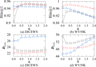
Figure 4. The result of GM-Decoder analysis

GM-Decoder formulates an objective $\bm{D}_{G_{s}G_{t}}$ to optimize the EA performance by transforming the EA problem into the graph matching problem. Ideally, the accuracy should be inversely proportional to $\bm{D}_{G_{s}G_{t}}$, meaning that the lower $\bm{D}_{G_{s}G_{t}}$, the better the EA performance. This aligns with the objective of minimizing the distance. To check whether it is the real situation, we proceed to evaluate the effectiveness of the GM-Decoder on finding optimal $\alpha$, by plotting the relation between the $\bm{D}_{G_{s}G_{t}}$ and the alignment performance. We vary $\alpha$ from 0 to 2 (cf. Section 5.1) in all three settings and record H@$1$ and $\bm{D}_{G_{s}G_{t}}$ of each step, as shown in Figure 4. First, we observe that H@$1$ is negatively correlated with $\bm{D}_{G_{s}G_{t}}$ for three settings, which validates the effectiveness of GM-Decoder in terms of finding the optimal $\alpha$. We also prove this in Table 4, where we report the worst and best H@$1$ when varying $\alpha$. Table 4 shows that GM-Decoder finds the best $\alpha$ in all cases. Second, the performance becomes better when $\alpha$ drops in the Unsupervised setting. This is because the pseudo-seed used in Relational-Encoder is generated with Temporal-Encoder, indicating that the temporal information is already learned by the Relational-Encoder. Third, the Normal setting generally outperforms the Less seed setting. This confirms that with more seed alignment, the Relational-Encoder can capture more relational information. Finally, we observe that the optimal $\alpha$ for DICEWS is around $1$ while it is around $0.5$ for WY50K. This implies that the importance of temporal and relational information in DICEWS are almost the same, but that in WY50K are biased. This may be caused by the algorithm generating DICEWS (Xu et al., 2021), which duplicates the ICEWS05-15 dataset into two TKGs with almost identical distributions. Based on the comparison results, WY50K is fitter for real-world applications, where the amount of temporal and relational information is usually biased.

5.6. Scalability Study

To verify the scalability of DualMatch, we plot the running time of each component on DICEWS and WY50K in Figure 5, where Normal, Less, and Unsup denote the Normal setting, Less seed setting, and Unsupervised setting, respectively. Specifically, the components are (1) Relational-Encoder that trains a GNN model to encode relational information; (2) Temporal-Encoder that takes the TKG inputs and encode the temporal information; and (3) GM-Decoder that fuses the two encoded information to produce the alignment matrix. We observe that the running time taken by each component does not exceed $10^{3}$ seconds on both DICEWS and WY50K, which confirms the scalability of DualMatch on a large dataset. We also observe that the training time in the Unsupervised setting is significantly higher than that of other settings. This is because more training iterations are required for the unsupervised setting, where the amount of pseudo seeds is $7.0-8.2$ times larger than those in the normal setting. To further study the scalability of DualMatch, we also provide a scalability study based on sampling sub-graphs in Appendix E.

Table 4. The worst and best H@$1$ when varying $\alpha$

Settings	DICEWS				WY50K
	Worst	Best	DualMatch		Worst	Best	DualMatch
Normal	93.7	95.3	95.3		95.9	98.1	98.1
Less seed	90.3	95.3	95.3		88.4	94.7	94.7
Unsupervised	94.5	94.6	94.6		91.0	96.4	96.4

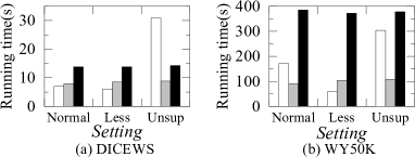
Figure 5. Scalability analysis vs. settings

6. Conclusions

In this study, we reinterpret the EA problem for TKGs as a weighted-graph-matching problem and investigate the potential for creating unsupervised methods for EA amongst TKGs by utilizing solitary relation triples with timestamps. We introduce DualMatch, which unsupervisedly aligns items by fusing relational and temporal data. The proposed DualMatch consists of two steps: (i) encode relational and temporal information independently into embeddings; and (ii) integrate both types of information and transform them into alignment using a novel graph-matching-based decoder. EA on TKGs can be performed using our technique with or without supervision. Furthermore, it does not require additional auxiliary information like entity names or pre-trained word embeddings necessary for earlier unsupervised EA techniques. Extensive experimental results on several real-world TKG datasets demonstrate that, even in the absence of training data, our technique significantly outperforms the state-of-the-art supervised methods. In the future, it is of interest to explore dangling settings (Sun et al., 2021) of EA on temporal datasets.

7. Acknowledgements

This work was supported in part by the National Key Research and Development Program of China under Grant No. 2021YFC3300303, the NSFC under Grants No. (62025206, 61972338, and 62102351), and the Ningbo Science and Technology Special Innovation Projects with Grant Nos. 2022Z095 and 2021Z019. Lu Chen is the corresponding author of the work.

Appendix A Example of Calculation

We provide a step-by-step example to clarify the calculation process depicted in Figure 2. We denote the two TKGs in Figure 2 as $G_{s}^{\star}$ and $G_{t}^{\star}$. First, we assign unique IDs to entities, relations, and timestamps, as shown in Table 5. Next, we count the outgoing edges by Equation 2 as well as the incoming edges and concatenate matrices. For simplicity, we omit the calculation of incoming edges and only demonstrate the process for outgoing edges as follows.

(8) $$\bm{A}^{t}=\begin{bmatrix}.40&.15&.15&.15&.15\\ .15&.15&.40&.15&.15\\ .15&.40&.15&.15&.15\\ .20&.20&.20&.20&.20\\ .15&.15&.15&.15&.40\\ .15&.15&.15&.40&.15\\ \end{bmatrix},$$

where $\bm{A}^{t}$ is the constructed $\bm{A}^{t}$ using $G_{s}^{\star}$. We proceed to build the relational adjacency matrix by Equation 3:

(9) $$\bm{A}=\begin{bmatrix}0&0&1&0&0&0\\ 0&0&1&0&0&0\\ 0&0&0&1&0&0\\ 0&0&0&0&0&0\\ 0&0&0&0&0&1\\ 0&0&0&0&1&0\\ \end{bmatrix}$$

The adjacency matrix $\bm{A}$ only contains $0$s and $1$s because each relation in Figure 2 only occurs once. As a result, they do not affect the numerical value of the adjacency matrix. By setting $L=1$, we obtain the temporal feature $\bm{H}^{t}$ which is the concatenation of $\bm{A}^{t}$ and $\bm{AA}^{t}$ (i.e., $\bm{H}^{t}=\left[\bm{A}^{t}||\bm{AA}^{t}\right]$):

(10) $$\bm{H}^{t}=\begin{bmatrix}.40&.15&.15&.15&.15&.15&.40&.15&.15&.15\\ .15&.15&.40&.15&.15&.15&.40&.15&.15&.15\\ .15&.40&.15&.15&.15&.20&.20&.20&.20&.20\\ .20&.20&.20&.20&.20&.00&.00&.00&.00&.00\\ .15&.15&.15&.15&.40&.15&.15&.15&.40&.15\\ .15&.15&.15&.40&.15&.15&.15&.15&.15&.40\end{bmatrix}$$

Then, we set $\bm{A}_{s}=\bm{A}_{t}=\bm{A}$ and $\bm{A}^{t}_{s}=\bm{A}^{t}_{t}=\bm{A}^{t}$ because $G_{s}^{\star}$ and $G_{t}^{\star}$ in Figure 2 are identical. This results in normalized WL weights $k^{r}=1$ and $k^{t}=1$. Since Relational-Encoder involves training of GNNs, we randomly initialize an embedding of $|E|\times 10$ for simplicity:

(11) $$\bm{H}^{r}_{s}=\bm{H}^{r}_{t}=\begin{bmatrix}.30&.44&.33&.40&.61&.35&.70&.85&.32&.56\\ .81&.61&.97&.84&.53&.00&.76&.44&.19&.45\\ .44&.51&.70&.72&.59&.21&.38&.88&.90&.67\\ .13&.21&.77&.25&.44&.71&.66&.37&.35&.61\\ .33&.33&.70&.29&.79&.51&.78&.60&.24&.59\\ .65&.94&.77&1.00&.50&.56&.50&.38&.54&.34\\ \end{bmatrix}$$

By setting the weight of Relational-Encoder to $0$, the alignment matrix $\bm{P}_{T}$ is solely determined by the temporal feature:

(12) $$\bm{P}_{T}=\bm{H}^{t}(\bm{H}^{t})^{T}=\begin{bmatrix}.50&.44&.39&.20&.37&.37\\ .44&.50&.39&.20&.37&.37\\ .39&.39&.45&.20&.39&.39\\ .20&.20&.20&.20&.20&.20\\ .37&.37&.39&.20&.50&.37\\ .37&.37&.39&.20&.37&.50\\ \end{bmatrix}$$

With $\bm{P}_{T}$, we obtain $\bm{D}_{G_{s}^{\star}G_{t}^{\star}}=4.61$ by Equation 6. Note that, we don’t consider Sinkhorn iteration and other processes except dot product for simplicity.

Similarly, by setting the weights of both Temporal-Encoder and Relational-Encoder to $1$, $\bm{P}$, the alignment matrix obtained by balancing temporal and relational features, is calculated as follows:

(13) $$\bm{P}=\bm{H}^{t}(\bm{H}^{t})^{T}+\bm{H}^{r}_{s}(\bm{H}^{r}_{t})^{T}=\begin{bmatrix}2.70&2.72&3.00&2.24&2.72&2.81\\ 2.72&3.97&3.41&2.42&2.98&3.75\\ 3.00&3.41&4.03&2.59&3.02&3.67\\ 2.24&2.42&2.59&2.49&2.61&2.60\\ 2.72&2.98&3.02&2.61&3.04&2.97\\ 2.81&3.75&3.67&2.60&2.97&4.26\\ \end{bmatrix}$$

This leads to $\bm{D}_{G_{s}^{\star}G_{t}^{\star}}=667.57$, which is significantly larger than 4.61. This suggests that a lower weight should be assigned to Relational-Encoder. In this case, as the relational feature was randomly generated, it would be more appropriate to give greater consideration to the temporal feature. Using only Temporal-Encoder would result in a H@1 of 100%, whereas using both Temporal-Encoder and Relational-Encoder with weights of 1 would decrease H@1 to 66.7%. This is consistent with the observed distance value.

Table 5. The ID allocation of Example TKG $G_{s}^{\star}$ and $G_{t}^{\star}$

ID	Name	Type
0	Federal Judge (Argentina)	Entities
1	Nordic Council
2	France
3	Javier Solana
4	Japan
5	Head of Government (Ukraine)
0	Reject judicial cooperation	Relations
1	Make an appeal or request
2	Sign formal agreement
3	Host a visit
4	Make a visit
0	2010-04-24	Timestamps
1	2007-09-29
2	2005-04-16
3	2007-05-10
4	2005-07-20

Appendix B Dataset Statistics

The comprehensive information of all datasets , including DICEWS, WY50K, and WY20K is shown in Table 6.

• DICEWS is generated from ICEWS05-15 (García-Durán et al., 2018), which is a subset of facts from the larger ICEWS (Lautenschlager et al., 2015) covering the time period from 2005 to 2015. ICEWS05-15 (García-Durán et al., 2018) is widely utilized as a benchmark for TKG comparisons in the community (Jain et al., 2020). The data generation is followed the method in (Zhu et al., 2017). The dataset contains 8,566 entity pairs and all of its facts include temporal information. The overlap ratio of shared quadruples between two TKGs $Q_{s}$ and $Q_{t}$ in DICEWS is approximately 50%, i.e. $2*\frac{|Q_{s}\cap Q_{t}|}{|Q_{s}|+|Q_{t}|}\approx 0.5$.

• WY50K is extracted from Wikidata (Vrandecic and Krötzsch, 2014) and YAGO (Suchanek et al., 2007). WY50K contains 49,172 entity pairs and all of its facts have temporal information.

• WY20K is also extracted from Wikidata (Vrandecic and Krötzsch, 2014) and YAGO (Suchanek et al., 2007). However, different from WY50K, WY20K is a hybrid dataset with 19,462 entity pairs, where 17.5% of YAGO’s facts and 36.6% of Wikidata’s facts do not have temporal information.

Appendix C Scalability Study on Sampled Datasets

To further study the scalability of DualMatch, we follow (Ge et al., 2022) to sample sub-graphs from DICEWS and WY50K. We vary the number of entities from 20% to 100% and record the running time (seconds) in Table 7, where R, T, and D represent Relational-Encoder, Temporal-Encoder and GM-Decoder, respectively. The results indicate that DualMatch is highly scalable. In particular, the running time increases at a quadratic rate as the number of entities increases, which is expected due to the quadratic time complexity of Sinkhorn algorithm. Despite this, even when 100% of the entities are used, the running time remains relatively short, taking 7 seconds for the Relational-Encoder, 7.9 seconds for the Temporal-Encoder, and 13.8 seconds for the GM-Decoder on DICEWS and taking 171.1 seconds for the Relational-Encoder, 90.2 seconds for the Temporal-Encoder, and 385.2 seconds for the GM-Decoder on WY50K. Note that the running time for the different components of DualMatch vary, with the GM-Decoder having the highest running time. This highlights the potential for optimization in the decoding process to further enhance the scalability of the entire DualMatch.

Overall, the scalability study demonstrates that DualMatch is capable of processing large datasets, as it exhibits a relatively low running time even when handling large-scale data. This makes DualMatch well-suited for real-world applications that require efficient and effective data processing.

Appendix D Open-world Entity Alignment

Most KGs in the real-world are dynamic, with new entities and timestamps emerging over time (Xu et al., 2022).This makes open-world entity alignment a critical task. However, most existing EA methods adopt a closed-world assumption and are unable to align newly emerging entities(Mao et al., 2020b, 2021a; Gao et al., 2022; Ge et al., 2021a; Liu et al., 2020). TREA (Xu et al., 2022) learns the embeddings of timestamps so that they may satisfy a specific mapping function from actual timestamps, thereby enabling EA on new entities. However, it can only roughly estimate future timestamp embeddings, which may result in errors for subsequent predictions. On the other hand, DualMatch is primarily unsupervised and can be readily adapted to open-world entity alignment by directly applying the unsupervised component online. As new entities and timestamps become available, Temporal-Encoder and GM-Decoder can then be re-executed to deliver the most accurate results.

To evaluate the open-world effectiveness of EA, we re-arrange the quadruples of DICEWS according to the open-world setting in TREA (Xu et al., 2022). The two training sets, $G_{s}^{\prime}$ and $G_{t}^{\prime}$, contain quadruples from $G_{s}$ and $G_{t}$ in DICEWS covering data prior to Jan. 1, 2014. We train Relational-Encoder with 1,000 randomly sampled pairs from $G_{s}^{\prime}$ and $G_{t}^{\prime}$ following (Xu et al., 2022). The embeddings of unseen entities and relations are initialized randomly.

We compare DualMatch with three state-of-the-arts: TREA (Xu et al., 2022), TEA-GNN (Xu et al., 2021), and RREA (Mao et al., 2020b). The results are shown in Table 8. DualMatch outperforms the baselines significantly in open-world EA with a $43.2\%$ increase in H@$1$ for unobserved entity pairs and a $34.9\%$ increase in H@$1$ for observed entity pairs. This is because both Temporal-Encoder and GM-Decoder of DualMatch are unsupervised and can be readily deployed online without training.

Appendix E Case Study

We perform a case study of TKG alignment using DualMatch, DualMatch-wt, and DualMatch-wr on DICEWS (denoted as $G_{s}^{\heartsuit}$ and $G_{t}^{\heartsuit}$), where DualMatch-wt denotes DualMatch without Temporal encoder and DualMatch-wt denotes DualMatch without Relational encoder. Given the ground truth $\{$(Abderrahim, Abderrahim), (Looter, Looter)$\}$, the results delivered by DualMatch are exactly the same as the ground truths. The results generated by DualMatch-wt and DualMatch-wr are detailed as follows.

Table 6. Statistics of DICEWS, WY50K, and WY20K

Dataset	#Entities	#Rels	#Time	#Quadruples
DICEWS	9,517-9,537	247-246	4,017	307,552-307,553
WY50K	49,629-49,222	11-30	245	221,050-317,814
WY20K	19,493-19,929	32-130	405	83,583-142,568

Table 7. The result of scalability analysis

	DICEWS					WY50K
	20%	40%	60%	80%	100%	20%	40%	60%	80%	100%
R	1.1	1.5	3.1	4.6	7.0	6.0	20.9	48.5	92.1	171.1
T	0.7	1.9	3.3	5.1	7.9	2.4	10.3	26.0	52.5	90.2
D	1.2	3.1	5.1	7.9	13.8	25.2	80.7	158.6	250.6	385.2

Table 8. The result of open-world entity alignment

Method	Unobserved Entity Pairs				Observed Entity Pairs
	H@1	H@10	MRR		H@1	H@10	MRR
DualMatch	77.4	89.5	0.829		94.2	96.6	0.952
TREA	34.2	74.8	0.479		54.9	82.5	0.643
TEA-GNN	15.5	59.0	0.324		39.2	74.8	0.513
RREA	7.5	48.3	0.253		36.1	58.0	0.407

For entity “Abderrahim” in $G_{s}^{\heartsuit}$, DualMatch correctly aligns it to “Abderrahim” in $G_{t}^{\heartsuit}$, while DualMatch-wr produces an incorrect alignment result “Chief”. The related quadruple of “Abderrahim” in $G_{s}^{\heartsuit}$ is (Abderrahim, Sign formal agreement, Foreign, 2007-09-28) and the related quadruple of “Chief” in $G_{t}^{\heartsuit}$ is (Chief, Express intent to meet or negotiate, Angola, 2007-09-28). The above case demonstrates that the distinction between the two entities cannot be identified based solely on the timestamp 2007-09-28.

For entity “Looter” in $G_{s}^{\heartsuit}$, DualMatch correctly align it to “Looter” in $G_{t}^{\heartsuit}$, while DualMatch-wt produces an incorrect alignment result “Rioter”. The related quadruple of “Looter” in $G_{s}^{\heartsuit}$ is (Looter, Use unconventional violence, France, 2005-11-09) and the related quadruple of “Rioter” $G_{t}^{\heartsuit}$ is (Rioter, Use unconventional violence, Police, 2005-03-14). Although $G_{s}^{\heartsuit}$ and $G_{t}^{\heartsuit}$ have different triples, Relational-Encoder fails to distinguish them. This is because we only use 10% of the entity pairs for training the relational model, which can sometimes result in inaccuracies.

In conclusion, DualMatch-wt and DualMatch-wr differ from the ground truths significantly. This implies the necessity of developing and incorporating temporal and relational encoders.

References

- (1)
- Bordes et al. (2013) Antoine Bordes, Nicolas Usunier, Alberto García-Durán, Jason Weston, and Oksana Yakhnenko. 2013. Translating Embeddings for Modeling Multi-relational Data. In NeurIPS. 2787–2795.
- Cao et al. (2019) Yixin Cao, Zhiyuan Liu, Chengjiang Li, Zhiyuan Liu, Juanzi Li, and Tat-Seng Chua. 2019. Multi-Channel Graph Neural Network for Entity Alignment. In ACL. 1452–1461.
- Chen et al. (2021) Muhao Chen, Weijia Shi, Ben Zhou, and Dan Roth. 2021. Cross-lingual entity alignment with incidental supervision. (2021), 645–658.
- Chen et al. (2017) Muhao Chen, Yingtao Tian, Mohan Yang, and Carlo Zaniolo. 2017. Multilingual Knowledge Graph Embeddings for Cross-lingual Knowledge Alignment. In IJCAI. 1511–1517.
- Cuturi (2013) Marco Cuturi. 2013. Sinkhorn Distances: Lightspeed Computation of Optimal Transport. In NeurIPS. 2292–2300.
- Gao et al. (2022) Yunjun Gao, Xiaoze Liu, Junyang Wu, Tianyi Li, Pengfei Wang, and Lu Chen. 2022. ClusterEA: Scalable Entity Alignment with Stochastic Training and Normalized Mini-batch Similarities. In KDD. 421–431.
- García-Durán et al. (2018) Alberto García-Durán, Sebastijan Dumancic, and Mathias Niepert. 2018. Learning Sequence Encoders for Temporal Knowledge Graph Completion. In EMNLP. 4816–4821.
- Ge et al. (2021a) Congcong Ge, Xiaoze Liu, Lu Chen, Baihua Zheng, and Yunjun Gao. 2021a. Make It Easy: An Effective End-to-End Entity Alignment Framework. In SIGIR. 777–786.
- Ge et al. (2022) Congcong Ge, Xiaoze Liu, Lu Chen, Baihua Zheng, and Yunjun Gao. 2022. LargeEA: Aligning Entities for Large-scale Knowledge Graphs. PVLDB 15, 2 (2022), 237–245.
- Ge et al. (2021b) Congcong Ge, Pengfei Wang, Lu Chen, Xiaoze Liu, Baihua Zheng, and Yunjun Gao. 2021b. CollaborEM: A Self-supervised Entity Matching Framework Using Multi-features Collaboration. TKDE (2021).
- Gold and Rangarajan (1996) Steven Gold and Anand Rangarajan. 1996. A Graduated Assignment Algorithm for Graph Matching. TPAMI 18, 4 (1996), 377–388.
- Hamilton et al. (2017) William L Hamilton, Rex Ying, and Jure Leskovec. 2017. Inductive representation learning on large graphs. In NeurIPS. 1025–1035.
- Harold W. Kuhn (1955) Harold W. Kuhn. 1955. The Hungarian method for the assignment problem. Naval Research Logistics Quarterly 2, 1, 83–97.
- Hu et al. (2021a) Xuming Hu, Fukun Ma, Chenyao Liu, Chenwei Zhang, Lijie Wen, and Philip S Yu. 2021a. Semi-supervised Relation Extraction via Incremental Meta Self-Training. In Findings of EMNLP. 487–496.
- Hu et al. (2020) Xuming Hu, Lijie Wen, Yusong Xu, Chenwei Zhang, and Philip S. Yu. 2020. SelfORE: Self-supervised Relational Feature Learning for Open Relation Extraction. In EMNLP. 3673–3682.
- Hu et al. (2021b) Xuming Hu, Chenwei Zhang, Yawen Yang, Xiaohe Li, Li Lin, Lijie Wen, and Philip S. Yu. 2021b. Gradient Imitation Reinforcement Learning for Low Resource Relation Extraction. In EMNLP. 2737–2746.
- Jain et al. (2020) Prachi Jain, Sushant Rathi, Mausam, and Soumen Chakrabarti. 2020. Temporal Knowledge Base Completion: New Algorithms and Evaluation Protocols. In EMNLP. 3733–3747.
- Jiang et al. (2022a) Chengyue Jiang, Wenyang Hui, Yong Jiang, Xiaobin Wang, Pengjun Xie, and Kewei Tu. 2022a. Recall, Expand and Multi-Candidate Cross-Encode: Fast and Accurate Ultra-Fine Entity Typing. arXiv preprint arXiv:abs/2212.09125 (2022).
- Jiang et al. (2022b) Chengyue Jiang, Yong Jiang, Weiqi Wu, Pengjun Xie, and Kewei Tu. 2022b. Modeling Label Correlations for Ultra-Fine Entity Typing with Neural Pairwise Conditional Random Field. arXiv preprint arXiv:2212.01581 (2022).
- Kipf and Welling (2017) Thomas N. Kipf and Max Welling. 2017. Semi-Supervised Classification with Graph Convolutional Networks. In ICLR.
- Lample et al. (2018) Guillaume Lample, Alexis Conneau, Marc’Aurelio Ranzato, Ludovic Denoyer, and Hervé Jégou. 2018. Word translation without parallel data. In ICLR.
- Lautenschlager et al. (2015) Jennifer Lautenschlager, Steve Shellman, and Michael Ward. 2015. ICEWS Event Aggregations. https://doi.org/10.7910/DVN/28117
- Li et al. (2019) Chengjiang Li, Yixin Cao, Lei Hou, Jiaxin Shi, Juanzi Li, and Tat-Seng Chua. 2019. Semi-supervised Entity Alignment via Joint Knowledge Embedding Model and Cross-graph Model. In EMNLP. 2723–2732.
- Li et al. (2021) Tianyi Li, Lu Chen, Christian S Jensen, and Torben Bach Pedersen. 2021. TRACE: Real-time compression of streaming trajectories in road networks. PVLDB 14, 7 (2021), 1175–1187.
- Li et al. (2020) Tianyi Li, Ruikai Huang, Lu Chen, Christian S Jensen, and Torben Bach Pedersen. 2020. Compression of uncertain trajectories in road networks. PVLDB 13, 7 (2020), 1050–1063.
- Liu et al. (2022b) Bing Liu, Wen Hua, Guido Zuccon, Genghong Zhao, and Xia Zhang. 2022b. High-quality Task Division for Large-scale Entity Alignment. arXiv preprint arXiv:2208.10366 (2022).
- Liu et al. (2021) Fangyu Liu, Muhao Chen, Dan Roth, and Nigel Collier. 2021. Visual Pivoting for (Unsupervised) Entity Alignment. In AAAI. 4257–4266.
- Liu et al. (2022a) Shuliang Liu, Xuming Hu, Chenwei Zhang, Shu’ang Li, Lijie Wen, and Philip S. Yu. 2022a. HiURE: Hierarchical Exemplar Contrastive Learning for Unsupervised Relation Extraction. In NAACL. 5970–5980.
- Liu et al. (2020) Zhiyuan Liu, Yixin Cao, Liangming Pan, Juanzi Li, and Tat-Seng Chua. 2020. Exploring and Evaluating Attributes, Values, and Structures for Entity Alignment. In EMNLP. 6355–6364.
- Mao et al. (2022) Xin Mao, Meirong Ma, Hao Yuan, Jianchao Zhu, ZongYu Wang, Rui Xie, Wei Wu, and Man Lan. 2022. An Effective and Efficient Entity Alignment Decoding Algorithm via Third-Order Tensor Isomorphism. In ACL. 5888–5898.
- Mao et al. (2021a) Xin Mao, Wenting Wang, Yuanbin Wu, and Man Lan. 2021a. Boosting the Speed of Entity Alignment 10: Dual Attention Matching Network with Normalized Hard Sample Mining. In WWW. 821–832.
- Mao et al. (2021b) Xin Mao, Wenting Wang, Yuanbin Wu, and Man Lan. 2021b. From Alignment to Assignment: Frustratingly Simple Unsupervised Entity Alignment. In EMNLP. 2843–2853.
- Mao et al. (2020a) Xin Mao, Wenting Wang, Huimin Xu, Man Lan, and Yuanbin Wu. 2020a. MRAEA: An Efficient and Robust Entity Alignment Approach for Cross-lingual Knowledge Graph. In WSDM. 420–428.
- Mao et al. (2020b) Xin Mao, Wenting Wang, Huimin Xu, Yuanbin Wu, and Man Lan. 2020b. Relational Reflection Entity Alignment. In CIKM. 1095–1104.
- Mena et al. (2018) Gonzalo E. Mena, David Belanger, Scott W. Linderman, and Jasper Snoek. 2018. Learning Latent Permutations with Gumbel-Sinkhorn Networks. In ICLR.
- Roth (2008) Alvin E Roth. 2008. Deferred acceptance algorithms: History, theory, practice, and open questions. international Journal of game Theory 36, 3 (2008), 537–569.
- Shervashidze et al. (2011) Nino Shervashidze, Pascal Schweitzer, Erik Jan van Leeuwen, Kurt Mehlhorn, and Karsten M. Borgwardt. 2011. Weisfeiler-Lehman Graph Kernels. JMLR 12 (2011), 2539–2561.
- Suchanek et al. (2007) Fabian M. Suchanek, Gjergji Kasneci, and Gerhard Weikum. 2007. Yago: a core of semantic knowledge. In WWW. 697–706.
- Sun et al. (2021) Zequn Sun, Muhao Chen, and Wei Hu. 2021. Knowing the No-match: Entity Alignment with Dangling Cases. In ACL. 3582–3593.
- Sun et al. (2020a) Zequn Sun, Muhao Chen, Wei Hu, Chengming Wang, Jian Dai, and Wei Zhang. 2020a. Knowledge Association with Hyperbolic Knowledge Graph Embeddings. In EMNLP. 5704–5716.
- Sun et al. (2017) Zequn Sun, Wei Hu, and Chengkai Li. 2017. Cross-Lingual Entity Alignment via Joint Attribute-Preserving Embedding. In ISWC. 628–644.
- Sun et al. (2018) Zequn Sun, Wei Hu, Qingheng Zhang, and Yuzhong Qu. 2018. Bootstrapping Entity Alignment with Knowledge Graph Embedding. In IJCAI. 4396–4402.
- Sun et al. (2020b) Zequn Sun, Chengming Wang, Wei Hu, Muhao Chen, Jian Dai, Wei Zhang, and Yuzhong Qu. 2020b. Knowledge Graph Alignment Network with Gated Multi-Hop Neighborhood Aggregation. In AAAI. 222–229.
- Sun et al. (2020c) Zequn Sun, Qingheng Zhang, Wei Hu, Chengming Wang, Muhao Chen, Farahnaz Akrami, and Chengkai Li. 2020c. A Benchmarking Study of Embedding-based Entity Alignment for Knowledge Graphs. PVLDB 13, 11 (2020), 2326–2340.
- Trisedya et al. (2019) Bayu Distiawan Trisedya, Jianzhong Qi, and Rui Zhang. 2019. Entity Alignment between Knowledge Graphs Using Attribute Embeddings. In AAAI. 297–304.
- Velickovic et al. (2018) Petar Velickovic, Guillem Cucurull, Arantxa Casanova, Adriana Romero, Pietro Liò, and Yoshua Bengio. 2018. Graph Attention Networks. In ICLR.
- Vrandecic and Krötzsch (2014) Denny Vrandecic and Markus Krötzsch. 2014. Wikidata: a free collaborative knowledgebase. Commun. ACM 57, 10 (2014), 78–85.
- Wang et al. (2022) Pengfei Wang, Xiaocan Zeng, Lu Chen, Fan Ye, Yuren Mao, Junhao Zhu, and Yunjun Gao. 2022. PromptEM: Prompt-tuning for Low-resource Generalized Entity Matching. PVLDB 16, 2 (2022), 369–378.
- Wang et al. (2018) Zhichun Wang, Qingsong Lv, Xiaohan Lan, and Yu Zhang. 2018. Cross-lingual Knowledge Graph Alignment via Graph Convolutional Networks. In EMNLP. 349–357.
- Weisfeiler and Leman (1968) Boris Weisfeiler and Andrei Leman. 1968. The reduction of a graph to canonical form and the algebra which appears therein. NTI, Series 2, 9 (1968), 12–16.
- Xin et al. (2022) Kexuan Xin, Zequn Sun, Wen Hua, Wei Hu, Jianfeng Qu, and Xiaofang Zhou. 2022. Large-scale Entity Alignment via Knowledge Graph Merging, Partitioning and Embedding. arXiv preprint arXiv:2208.11125 (2022).
- Xiong et al. (2017) Chenyan Xiong, Russell Power, and Jamie Callan. 2017. Explicit Semantic Ranking for Academic Search via Knowledge Graph Embedding. In WWW. 1271–1279.
- Xu et al. (2021) Chengjin Xu, Fenglong Su, and Jens Lehmann. 2021. Time-aware Graph Neural Network for Entity Alignment between Temporal Knowledge Graphs. In EMNLP. 8999–9010.
- Xu et al. (2022) Chengjin Xu, Fenglong Su, Bo Xiong, and Jens Lehmann. 2022. Time-aware Entity Alignment using Temporal Relational Attention. In WWW. 788–797.
- Yu et al. (2021) Donghan Yu, Yiming Yang, Ruohong Zhang, and Yuexin Wu. 2021. Knowledge Embedding Based Graph Convolutional Network. In WWW. 1619–1628.
- Zeng et al. (2022) Weixin Zeng, Xiang Zhao, Xinyi Li, Jiuyang Tang, and Wei Wang. 2022. On entity alignment at scale. VLDBJ (2022), 1–25.
- Zeng et al. (2020) Weixin Zeng, Xiang Zhao, Jiuyang Tang, and Xuemin Lin. 2020. Collective Entity Alignment via Adaptive Features. In ICDE. 1870–1873.
- Zhang et al. (2022) Xin Zhang, Guangwei Xu, Yueheng Sun, Meishan Zhang, Xiaobin Wang, and Min Zhang. 2022. Identifying Chinese Opinion Expressions with Extremely-Noisy Crowdsourcing Annotations. In ACL. 2801–2813.
- Zhang et al. (2021) Xin Zhang, Guangwei Xu, Yueheng Sun, Meishan Zhang, and Pengjun Xie. 2021. Crowdsourcing Learning as Domain Adaptation: A Case Study on Named Entity Recognition. In ACL. 5558–5570.
- Zhu et al. (2017) Hao Zhu, Ruobing Xie, Zhiyuan Liu, and Maosong Sun. 2017. Iterative Entity Alignment via Joint Knowledge Embeddings. In IJCAI. 4258–4264.