Generative Modeling with Quantum Neurons

Abstract

The recently proposed Quantum Neuron Born Machine (QNBM) has demonstrated quality initial performance as the first quantum generative machine learning (ML) model proposed with non-linear activations. However, previous investigations have been limited in scope with regards to the model’s learnability and simulatability. In this work, we make a considerable leap forward by providing an extensive deep dive into the QNBM’s potential as a generative model. We first demonstrate that the QNBM’s network representation makes it non-trivial to be classically efficiently simulated. Following this result, we showcase the model’s ability to learn (express and train on) a wider set of probability distributions, and benchmark the performance against a classical Restricted Boltzmann Machine (RBM). The QNBM is able to outperform this classical model on all distributions, even for the most optimally trained RBM among our simulations. Specifically, the QNBM outperforms the RBM with an improvement factor of $75.3$x, $6.4$x, and $3.5$x for the discrete Gaussian, cardinality-constrained, and Bars and Stripes distributions respectively. Lastly, we conduct an initial investigation into the model’s generalization capabilities and use a KL test to show that the model is able to approximate the ground truth probability distribution more closely than the training distribution when given access to a limited amount of data. Overall, we put forth a stronger case in support of using the QNBM for larger-scale generative tasks.

I Introduction

Quantum models for machine learning (ML) tasks is a promising area of research that aims to understand the potential advantages that quantum computers exhibit over their classical counterparts for practical data-driven applications Cerezo et al. (2022); Perdomo-Ortiz et al. (2018); Schuld and Killoran (2022). This field, known as quantum machine learning (QML) has split into multiple areas of research, including the type of input data (classical Zoufal et al. (2019); Rudolph et al. (2020); Sarma et al. (2019) or quantum Caro et al. (2021); Carrasquilla et al. (2019); Poland et al. (2020)), the training algorithm (supervised Maria Schuld (2018) or unsupervised Lloyd et al. (2013)), and the approach for evaluation (application benchmarking Zhu et al. (2019); Gili et al. (2022a); Alcazar et al. (2020) or Statistical Learning Theory Sammut and Webb (2011); Hinsche et al. (2021, 2022)).

One of the most relevant research directions for achieving quantum advantage in the field of QML is unsupervised generative modeling. The goal of an unsupervised generative model is to learn the underlying probability distribution from an unlabeled training set such that it can generate new high quality data Gui et al. (2020); Ruthotto and Haber (2021). Industry-scale classical generative models are deployed for applications in recommendations systems Cheng et al. (2016), image restoration Basioti and Moustakides (2020), portfolio optimization Alcazar and Perdomo-Ortiz (2021), and drug discovery Brown et al. (2019). Developing and characterizing more powerful generative models is of utmost importance for realizing the most advanced Artificial Intelligence applications Gm et al. (2020).

Quantum circuits can represent a probability distribution over a support of discrete bitstrings and each quantum measurement in the computational basis is akin to generating a sample Benedetti et al. (2019a). Thus, designing these parameterized circuits for generative modeling tasks is a natural idea. We also have theoretical evidence that generative models with certain quantum gate structures have more expressive power than classical networks Du et al. (2020). However, the optimal design of these models for both NISQ and fault-tolerant hardware regimes is an open question. With each new proposed architecture, a thorough investigation into the model’s learning capabilities is necessary to understand its strengths and limitations as a candidate for practical quantum advantage.

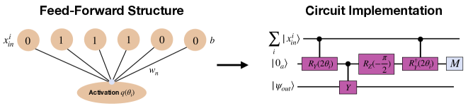
Figure 1: Visual demonstration of mapping information to a single output neuron in the QNBM. On the left, we show the feed-forward structure of the neuron activation, which closely resembles a classical network containing trainable weights $w_{n}$ and biases $b$ on individual bitstrings $x^{i}_{in}$. The activation function $q$ introduces non-linearity to the output neuron in the next layer. To the right, we show the quantum circuit implementation that produces this non-linear mapping in the form of a quantum RUS circuit. The circuit feeds forward information from the superposition of bitstrings in the input layer $\sum_{i}|x_{in}\rangle$ and performs the non-linaer activation on one output neuron $|\psi_{out}\rangle$. The QNBM is simply a multi-layered network comprised of these individual quantum neuron activations. Note that a main difference between the classical structure (left) and the quantum circuit model (right) is that the quantum network allows for a superposition of inputs in the initial layer.

Recently, the first quantum generative model with non-linear activations was introduced to the literature, known as the Quantum Neuron Born Machine (QNBM) Gili et al. (2022b). This work put forth a preliminary investigation into the model’s learning capabilities, along with a demonstration of superior performance over the more widely investigated Quantum Circuit Born Machine (QCBM) Benedetti et al. (2019b); Liu and Wang (2018); Coyle et al. (2020); Gili et al. (2022c). As the QNBM is able to incorporate non-linearity into its state evolution through mid-circuit measurements, it may contain many advantages that are yet to be discovered.

Following the initial proposal of the model, many important questions remained open. For example, is the model efficiently classically simulatable? Can the model learn (express and effectively train on) a wider set of distributions? How does the model’s learning performance compare to a similar classical model? And lastly, can the model generalize when given access to a finite number of samples from the target probability distribution?

In this work, we tackle answering these questions, providing an extensive investigation into the QNBM as a generative model. First, we show that the QNBM’s network representation makes it non-trivial to efficiently simulate classically. We then provide results demonstrating the QNBM’s ability to learn a more diverse set of distributions, and benchmark it against the Restricted Boltzmann Machine (RBM) Montufar (2018), a comparable classical model. We show that the QNBM is able to outperform the RBM by a large margin on all distributions, even for the most optimally trained RBM. Lastly, we conduct an initial investigation into the model’s generalization capabilities. Using a simple KL test, we show that the model is able to get closer to the true distribution than the training distribution when given access to a limited training set. In summary, we provide substantial evidence regarding the QNBM’s power as a generative model, highlighting the importance of conducting further investigations for practical applications once the required hardware becomes available.

II Generative Models

The goal of an unsupervised generative model is to learn an unknown probability distribution $P_{target}$ from a finite set of data such that it can generate new samples from the same underlying distribution Gui et al. (2020); Ruthotto and Haber (2021); Zhao et al. (2018); Gili et al. (2022d). Prior to demonstrating the results gathered from our deep-dive investigation into the QNBM, we provide an overview of the model’s circuit structure and training scheme. Additionally, we provide a brief summary of the RBM model, which we utilize for classical benchmarking.

II.1 Quantum Neuron Born Machine (QNBM)

The QNBM is a quantum analogue of a classical feed-forward neural network, introduced in Gili et al. Gili et al. (2022b). Each neuron in the network is assigned a qubit and is connected to the previous layer of neurons via a quantum neuron sub-routine Cao et al. (2017), which is a Repeat-Until-Success (RUS) circuit Bocharov et al. (2015); Paetznick and Svore (2013); Quantum_arithmetic; Wiebe and Roetteler (2014). The quantum neuron sub-routine is comprised of an input register $\ket{x_{in}}$ representing the previous layer of neurons, an output qubit initiated in the state $\ket{\psi_{out}}$ representing the neuron of the next layer, and also an ancilla qubit, initially in $\ket{0_{a}}$. The ancilla is used for mapping activation functions from the input layer of neurons $|x_{in}\rangle$ to each output neuron $\ket{\psi_{out}}$ in the next layer. A visual representation of the RUS sub-routine for a single neuron is demonstrated in Figure 1.

The RUS circuit performs a non-linear activation function at each output neuron after summing up the weights and biases from the neurons in the previous layer. Thus, each tunable parameter $\theta$ is a function of weights and biases:

$$\theta=w_{1}x_{1}+w_{2}x_{2}+...+w_{n}x_{n}+b,$$ (1)

where ${w_{n}}\in(-1;1)$ are the weights for $n$ neurons in the previous layer and $b\in(-1;1)$ is the bias. Through mid-circuit measurements of the ancilla, the following activation function is enacted:

$$q(\theta)=\arctan(\tan^{2}(\theta)).$$ (2)

This non-linear activation function contains a sigmoid shape, making it comparable to those typically used in classical neural networks. By measuring the ancilla qubit to be $\ket{0_{a}}$, which occurs with a probability $p(\theta)>\frac{1}{2}$ Cao et al. (2017), we perform the activation function on the output neuron. Otherwise, the activation function is not enacted and we must recover the pre-circuit state with an $X$ gate on the ancilla and $R_{Y}(-\pi/2)$ applied to the output qubit. The process will then be repeated until the ancilla measurement yields $\ket{0_{a}}$.

The final state of each output neuron with a successful activation can be described as:

$$\sum_{i}F_{i}|x^{i}_{in}\rangle\otimes|0_{a}\rangle\otimes R_{Y}q(2\theta_{i})|\psi_{out}\rangle,$$ (3)

where $F_{i}$ is refers to an amplitude deformation in the input state during the RUS mapping and $\theta_{i}$ is the sum of weights and biases for each input bitstring. Note that due to the $R_{Y}$ rotation, the total function enacted on the output node is $\sin^{2}(q(2\theta_{i}))$. A key difference between the QNBM and classical neural networks is its ability to perform an activation function on a superposition of discrete bitstrings $\sum_{i}\ket{x^{i}_{in}}$.

QNBMs are defined by their neuron structure, i.e. the number of neurons in each layer $(N_{in},N_{hid},...,N_{out})$. At the end of the circuit, samples are drawn from the model according to the Born Rule when measuring only the output neurons. These samples are used to approximate the model’s encoded probability distribution, i.e. $P_{model}$.

The QNBM is trained with a classical optimizer to minimize the KL Divergence between $P_{target}$ and $P_{model}$ with a finite differences gradient estimator. Samples are generated post training for a separate evaluation of the model’s ability to learn the desired distribution. This training scheme is very similar to other quantum generative models like QCBMs Liu and Wang (2018) and tensor networks Han et al. (2018).

II.2 Restricted Boltzmann Machine (RBM)

The classical RBM architecture contains two layers of neurons: the visible layer $v_{i}$ and the hidden layer $h_{j}$. The neurons in these layers are connected in a bipartite structure Montufar (2018). The model learns each neuron’s weight $w_{i,j}$ and each layer’s bias $a_{i},b_{j},$ throughout training, where the number of parameters is defined by the number of visible units $V$ and hidden units $H$.

The model is trained with a Stochastic Divergence method called Contrastive Divergence. Through this training, discrete bitstrings sampled from the target distribution are fed to the model, and then the joint probability distribution is learned over the visible and hidden units by approximating their conditional probability distributions via a Gibbs Sampling Montufar (2018) method. These individual conditional probability distributions are defined by:

$$\begin{split}P(h_{j}=1|v)=\sigma(b_{j}+\sum_{i=1}^{V}w_{i,j}{v_{i}}),\\ P(v_{i}=1|h)=\sigma(a_{i}+\sum_{j=1}^{H}w_{i,j}h_{j}),\end{split}$$ (4)

where $\sigma$ is the logistic sigmoid activation function.

Samples from these conditional distributions allow one to approximate the gradient, where a gradient descent procedure is then used to compute and update the parameters throughout training.

III Results

In this section, we introduce a deeper investigation into the QNBM as a quantum generative model from multiple perspectives. First, we investigate how the neural network structure of the QNBM affects its classical simulatability, comparing the non-linear model to its ”linearized” version. Next, we thoroughly assess the model’s learning capabilities by training a $(5,0,6)$ network on three types of target probability distributions. To further distinguish the quantum model’s capabilities from those of classical generative architectures, we benchmark the learning performance against a classical RBM, which contains a similar network structure to the QNBM with a similar number of resources. Lastly, we provide the first demonstration of the model’s ability to generalize - i.e. learn an underlying ground truth probability distribution from a limited number of training samples.

III.1 Classical Simulatability

The QNBM’s neural network connectivity is much more restrictive than many variational ansätze, prompting the question of whether it is efficiently classically simulatable. In this section, we provide some insight into this question by comparing the output of a QNBM to that of its ”linearized” counterpart, discussed in Gili et al. (2022b). We show that generating a sample from the linearized QNBM is akin to forward sampling in a Bayesian network. However, this behavior does not transfer to the non-linear QNBM trained in this work, which we see as strong evidence against the efficient simulatability of the QNBM.

Suppose we have a QNBM with $n$ layers, where the first $k<n$ layers are connected, and we want to connect a neuron in the $k+1$’th layer to the network. The combined state of the first $k$ layers, the qubit in the $k+1$’th layer, and the ancilla can be generally written as

$$\ket{\psi_{k+1}}=\left(\sum^{2^{N_{k}}}_{i=1}\alpha_{i}\ket{\phi_{i}}\otimes\ket{x_{i}}_{k}\right)\otimes\ket{0}_{k+1}\otimes\ket{0}_{a},$$ (5)

where each $\ket{\phi_{i}}$ describes the first $k-1$ layers, and each $\ket{x_{i}}$ is a single bitstring state representing the $k^{th}$ layer. Notice that if the network terminates at the $k^{th}$ layer, then the probabilities of the various output bitstrings $x_{i}$ are given by $|\alpha_{i}|^{2}$. By applying the gates as described in Section II.1, we get the pre-measurement state

$$\begin{split}\ket{\psi_{k+1}}=\sum^{2^{N_{k}}}_{i=1}\alpha_{i}\ket{\phi_{i}}\otimes\ket{x_{i}}_{k}\otimes(\cos^{2}{\theta_{i}}\ket{0}_{k+1}\otimes\ket{0}_{a}\\ +\sin{\theta_{i}}\cos{\theta_{i}}\ket{0}_{k+1}\otimes\ket{1}_{a}\\ +\sin{\theta_{i}}\cos{\theta_{i}}\ket{1}_{k+1}\otimes\ket{1}_{a}\\ +\sin^{2}{\theta_{i}}\ket{1}_{k+1}\otimes\ket{0}_{a}),\end{split}$$ (6)

where $\theta_{i}=(\sum^{2^{N_{k}}}_{j=1}w_{ij}x_{j})+b_{i}$ . If we measure the ancilla and obtain result zero, then up to normalization the state becomes

$$\begin{split}\ket{\psi_{k+1}}=\sum^{2^{N_{k}}}_{i=1}\alpha_{i}\ket{\phi_{i}}\otimes\ket{x_{i}}_{k}\otimes(\cos^{2}{\theta_{i}}\ket{0}_{k+1}\otimes\ket{0}_{a}\\ +\sin^{2}{\theta_{i}}\ket{1}_{k+1}\otimes\ket{0}_{a}).\end{split}$$ (7)

The probability of finding the connected neuron in the zero state and one state respectively become

$$P_{0}=\frac{\sum^{2^{N_{k}}}_{i=1}|\alpha_{i}|^{2}\cos^{4}{\theta_{i}}}{\sum^{2^{N_{k}}}_{i=1}|\alpha_{i}|^{2}(\cos^{4}{\theta_{i}}+\sin^{4}{\theta_{i}})},$$ (8)

$$P_{1}=\frac{\sum^{2^{N_{k}}}_{i=1}|\alpha_{i}|^{2}\cos^{4}{\theta_{i}}}{\sum^{2^{N_{k}}}_{i=1}|\alpha_{i}|^{2}(\cos^{4}{\theta_{i}}+\sin^{4}{\theta_{i}})}.$$ (9)

Let us compare these expressions to those from a ”linearized” QNBM, where quantum neuron sub-routines are simply replaced with unitary Pauli-Y rotations. If we connect a neuron in the $k+1^{th}$ layer to the $k^{th}$ layer of neurons (starting from the same state as before), we obtain

$$\begin{split}\ket{\psi_{k+1}}^{(lin)}=\sum^{2^{N_{k}}}_{i=1}\alpha_{i}\ket{\phi_{i}}\otimes\ket{x_{i}}_{k}\otimes(\cos{\theta_{i}}\ket{0}_{k+1}+\\ \sin{\theta_{i}}\ket{1}_{k+1}),\end{split}$$ (10)

such that

$$P_{0}^{(lin)}=\frac{\sum^{2^{N_{k}}}_{i=1}|\alpha_{i}|^{2}\cos^{2}{\theta_{i}}}{\sum^{2^{N_{k}}}_{i=1}|\alpha_{i}|^{2}(\cos^{2}{\theta_{i}}+\sin^{2}{\theta_{i}})}=\sum^{2^{N_{k}}}_{i=1}|\alpha_{i}|^{2}\cos^{2}{\theta_{i}},$$ (11)

$$P_{1}^{(lin)}=\frac{\sum^{2^{N_{k}}}_{i=1}|\alpha_{i}|^{2}\sin^{2}{\theta_{i}}}{\sum^{2^{N_{k}}}_{i=1}|\alpha_{i}|^{2}(\cos^{2}{\theta_{i}}+\sin^{2}{\theta_{i}})}=\sum^{2^{N_{k}}}_{i=1}|\alpha_{i}|^{2}\sin^{2}{\theta_{i}}.$$ (12)

Notice that the probabilities are linear combinations of the values $|\alpha_{i}|^{2}$ which also correspond to output bitstring probabilities if the network was terminated at layer $k$. Then the factors of $\cos^{2}{\theta_{i}}$ and $\sin^{2}{\theta_{i}}$ correspond to conditional probabilities. In other words,

$$P_{k+1}^{j}=\sum^{2^{N_{k}}}_{i=1}P(j|i)P(i)$$ (13)

where $P(j|i)$ means ”probability to find a neuron in the $k+1^{th}$ layer in state $j$, given that the neurons in the $k^{th}$ layer have been found in state $i$. The probabilities are $P(i)=|\alpha_{i}|^{2}$, $P(j|i)=\cos^{2}(\theta_{i})$ for $j=0$ and $P(j|i)=\sin^{2}(\theta_{i})$ for $j=1$.

Since we are able to write the probabilities $P^{(lin)}_{i}$ in this form, sampling bitstrings from the $k+1^{th}$ layer of the network is equivalent to the process of sampling bitstrings from the $k^{th}$ layer, classically calculating the probabilities for the $k+1^{th}$ layer, and then sampling it from those. The calculation of probabilities and subsequent sampling requires $O(E_{k\rightarrow k+1})$ calculations, where $E_{k\rightarrow k+1}$ is the number of edges connecting layers $k$ and $k+1$; therefore, such sampling is efficient. This is true for any pair of previously connected layers (Eq. (5) describes a completely general QNBM state), and as such, one can sample efficiently and classically from the whole network with $O(E)$ calculations, where $E$ is the number of edges in the whole network.

In fact, this construction is precisely a Bayesian network Cheng et al. (1997). Bayesian networks can be sampled from efficiently, and therefore the ”linearized” QNBM can be efficiently sampled from as well. Physically, this classical simulatability relies on the deferred measurement principle.

Clearly the same construction does not work for the non-linear QNBM as the probabilities for the connected neuron are not linear combinations of the output probabilities for the layer that precedes it, and so there are no well-defined ”conditional probabilities”. While there may be other classical models equivalent to the QNBM, we believe the connection is certainly very non-trivial. Therefore, the QNBM is likely not efficiently classically simulatable.

III.2 Distribution Learning

In this section, we assess the QNBM’s ability to effectively learn three target probability distributions typically utilized in the literature for benchmarking: Bars and Stripes (BAS), cardinality-constrained, and discrete Gaussian. Each distribution is defined on the set of $2^{N}$ bistrings. All simulations in our work are conducted with distributions of dimension $N=6$, as this constitutes the size of each network’s output layer. A BAS distribution is composed of uniform probabilities over bitstrings that represent either a bar or a stripe in a 2D binary grid. In this encoding, each binary digit represents a white $(0)$ or black square $(1)$ such that these patterns emerge Benedetti et al. (2019b). For an $N=6$ distribution with a $2\times 3$ grid, there are $20$ patterns for the model to learn Liu and Wang (2018). A cardinality-constrained distribution contains uniform probabilities over bitstrings that fit a given numerical constraint in the number of binary digits equivalent to $1$ (e.g. $"001011"$ has a cardinality of $3$). For a cardinality of $c=3$, we have ${6\choose 3}=20$ patterns for the model to learn. Lastly, for the discrete Gaussian, we simply ask the model to learn the function $f(x)=\frac{1}{\sigma\sqrt{2\Pi}}\exp(-\frac{1}{2}\frac{(x-\mu)^{2}}{\sigma^{2}})$, where $\mu$ is the chosen mean and $\sigma$ is the chosen standard deviation. For all simulations, the distributions are peaked at the central bitstring with $\sigma=7$, as these values were appropriate for the distribution support size.

For this first part of our learning investigation, we provide the model with complete access to the underlying probability distribution, rather than using a finite number of training samples. This method, prominently used in the literature to investigate alternative generative architectures such as Quantum Circuit Born Machines (QCBMs) Zhu et al. (2019); Benedetti et al. (2019b); Liu and Wang (2018), allows us to investigate two important attributes regarding the model’s ability to learn a wider range of distributions: the model’s expressivity and its ability to be effectively trained.

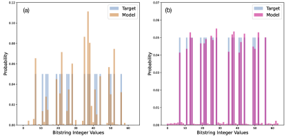
Figure 2: The RBM and QNBM learning performance on the Cardinality Constrained distribution. (a) RBM output probability distribution. (b) QNBM output probability distribution. The RBM and QNBM are able to achieve KL values of $KL=0.256$ and $KL=0.04$, respectively. We see that the QNBM outperforms the RBM by a $6.4$x improvement factor.

The model’s learning capability can be evaluated by computing the overlap of the model’s output probability distribution $P_{model}(x)$ with that of the target distribution $P_{target}(x)$. While there are many metrics that fulfil this purpose, it suffices for our small scale models to use the simple Kullback-Leibler Divergence Joyce (2011) defined as:

$$KL=\sum_{x}P_{target}(x)\log\left(\frac{P_{target}(x)}{\max(P_{model}(x),\epsilon)}\right),$$ (14)

where $\epsilon\approx 10^{-16}$ such that the function remains defined for $P_{model}(x)=0$. When assessing expressivity, the desire is to obtain the following:

$$KL(P_{target}(x),P_{model}(x))=0$$ (15)

This means that the model’s distribution is identical to the target, and thus the model can fully express the target distribution. Note that this evaluation provides no information about the model’s capacity to generalize as the model receives all of the data from the underlying distribution as input.

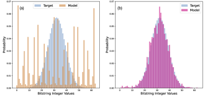
Figure 3: RBM and QNBM learning performance on a discrete Gaussian distribution. (a) RBM output probability distribution. (b) QNBM output probability distribution. The RBM and QNBM are able to achieve KL values of $KL=1.464$ and $KL=0.019$, respectively. We see that the QNBM outperforms the RBM by a $75.3$x improvement factor.

Here, we provide the distribution learning performance of a $(N_{in},N_{hid},N_{out})=(5,0,6)$ QNBM benchmarked against a $V=6,H=5$ RBM on the three distributions. These structures allow us to assign a similar number of parameters to each model (QNBM: 36 RBM: 41), and it has been shown in previous work that QNBMs at small scales perform optimally when no hidden layers on introduced Gili et al. (2022b). Both models start with small randomly initialized parameters. We keep the number of classical resources provided to each model as similar as possible by equating the number of shots taken by the QNBM with the number of Gibbs samples executed by the RBM throughout the training. This is an apt comparison because both shots and Gibbs samples are the most expensive resources for each model, and both broadly serve to query the model’s encoded distribution. With this constraint, we choose meta-parameters that enable each model to train optimally. More specifically, the QNBM is trained with $2,000$ iterations and $10,000$ shots per iteration, for a total of 20 million shots throughout the training. As the RBM utilizes resources differently than the QNBM in its training scheme, we trained our RBMs using two different approaches to ensure that we obtained a correct balance of distributed resources for obtaining optimal performance: the RBM-2k with $2\cdot 10^{3}$ iterations and $10^{4}$ shots per iteration, and the RBM-20k with $2\cdot 10^{4}$ iterations and $10^{3}$ shots per iteration. When simulating the QNBM, we utilize postselection rather than implement mid-circuit measurements with classical control for each RUS sub-routine. The number of shots quoted is the number of shots before postselection. In practice, a quantum device running the QNBM would require the capacity for mid-circuit measurements and classical control to avoid an exponential shot cost.

We report the values of the best performing model across $5$ independent trainings. Note that this includes the trials of both the RBM-2k and the RBM-20k. The QNBM is able to achieve very low KL values with $KL=0.04$ for the cardinality-contrained distribution, $KL=0.019$ for the discrete Gaussian distribution, and $KL=0.099$ for BAS. This is a $6.4$x, $75.3$x, and $3.5$x improvement factor over the RBM for each distribution respectively. The RBM is only able to achieve values of $KL=0.256$ on the cardinality-constrained distribution, $KL=1.464$ on the discrete Gaussian, and $KL=0.345$ on the BAS distribution. In Figure 2 and Figure 4, we see the distribution outputs for each model trained on the cardinality-constrained and the BAS distributions respectively. From these results we observe that the QNBM has high enough expressivity to represent these distributions and that it can be effectively trained to do so. Furthermore, we see that the QNBM is able to capture representational patterns in discrete bitstrings very well and achieves significant advantage over our RBM model. We see in Figure 3 that the RBM performs considerably worse on the Gaussian distribution, whereas the QNBM is able to capture both the high probability and the low probability bitstrings very well. Thus, we have demonstrated strong evidence that the QNBM is highly expressive and capable of capturing two very important types of patterns: representational features within discrete bitstrings distributed uniformly and distribution shapes that arise from non-uniformity over a support of discrete bitstrings.

While the QNBM is able to achieve quality learning performance across all distributions, it does not have the same stability in training on all three distributions, and is sometimes more unstable than the RBM. As shown in Appendix V.1, the model is much more stable on the cardinality-constrained distribution than the discrete Gaussian and BAS distributions. This instability suggests that it is important to run multiple independent trainings to achieve optimal performance. We leave the investigation into further understanding this model’s training instabilities for future work and discussion.

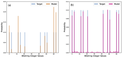
Figure 4: RBM and QNBM learning performance on the Bars and Stripes distribution. (a) RBM output probability distribution. (b) QNBM output probability distribution. The RBM and QNBM are able to achieve KL values of $KL=0.345$ and $KL=0.099$, respectively. We see that the QNBM outperforms the RBM by a $3.5$x improvement factor.

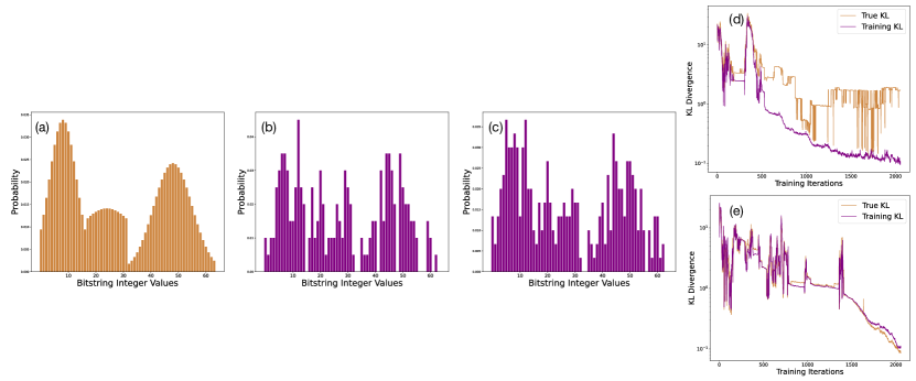
Figure 5: The QNBM’s generalization performance on various training distributions sampled from the ground truth. (a) The ground truth probability distribution $P_{true}(x)$. (b) A training distribution containing 200 samples from the true distributions, defined as $d_{200}$. (c) A training distribution containing 300 samples from the true distributions, defined as $d_{300}$. (d) The generalization performance for the training distribution $d_{200}$. (e) The generalization performance for the training distribution $d_{300}$. Throughout training, the model gets closer to both the ground truth and each training distribution, but for the training distribution $d_{300}$, the model’s True KL ($KL_{true}$) is able to dip below the Training KL $KL_{train}$ more consistently, providing more concrete evidence for generalization.

Lastly, we want to emphasize the importance of considering a balanced resource allocation method when comparing classical and quantum models. In the above learning results, the RBM-20k performs better than the RBM-2k in 2 out of 3 distributions. This indicates that the choices made in allocating a fixed number of resources to two different models (e.g. number of iterations vs shots per iteration) can significantly impact the results of their comparison. For this reason, it is generally important to ensure that resources are fairly allocated to each model when benchmarking or comparing them. Results demonstrating the difference between the RBM-2k and the RBM-20k for each distribution are displayed in Appendix V.1.

Overall, the QNBM is able to achieve impressive learning performance as a standalone model when given access to the underlying distribution during training. It maintains high expressivity and trainability across distribution types. We are able to further highlight the QNBM’s performance using a comparable RBM as a benchmark. Note that we are not using this evidence to claim that the QNBM is superior to all classical models or even to all potential RBM implementations, as we believe finding more theoretical bounds is necessary to make any such statements around quantum advantage. We believe deriving such theoretical bounds, while non-trivial, is important future work for obtaining the model’s limits on learnability, expressibility, and trainability.

III.3 Generalization Performance

We take one step further in understanding the QNBM’s learnability by assessing its generalization performance, i.e. its ability to learn an underlying distribution $P_{true}(x)$ from a finite number of training samples. This is in contrast to the previous section, where all models were trained on the underlying distribution itself.

We assess generalization performance using an approach previously detailed in the literature Gili et al. (2022c); Rudolph et al. (2021). This method consists of training the model on a finite number of samples from the underlying probability distribution and evaluating whether it can more closely approximate the true distribution from this limited training set. Concretely, at the end of the training, one can compare the overlap between the model and the training distribution $P_{train}$ with the overlap between the model and the true distribution $P_{true}$. If the model’s encoded distribution is closer to the true distribution than to the training distribution, one can conclude that the model has indeed generalized to the true distribution from the training set. Concretely, the model has generalized if:

$$\begin{split}KL(P_{true}(x),P_{model}(x))<\\ KL(P_{train}(x),P_{model}(x))\end{split}$$ (16)

We will refer to the term on the left side of the inequality as $KL_{true}$ and the term on the right side as $KL_{train}$.

We probe the QNBM’s ability to generalize samples from a superposition of three univariate Gaussian distributions. The three Gaussian distributions have means and variances $(\mu,\sigma)$ of $(8,5)$, $(24,12)$, and $(48,7)$. We take 200 and 300 samples from the underlying distribution to construct two different training distributions and refer to these distributions as $d_{200}$ and $d_{300}$ respectively. We show the underlying distribution as well as the two training distributions in Figure 5. Note that $KL(P_{true}(x),d_{200})=3.10$ and $KL(P_{true}(x),d_{300})=0.703$.

We train the (5,0,6) QNBM with $2\cdot 10^{3}$ iterations and $10^{4}$ shots per iteration on each training distribution. We ran the QNBM on each training distribution over five independent trials with randomly initialized parameters. Since one typically does not have access to $KL_{true}$ but can easily compute $KL_{train}$, we report the performance of the model on the trial with the lowest final $KL_{train}$ and assess the generalization performance. We provide numerical values from all trials in Appendix V. In Figure 5, we showcase the model’s training performance on this trial. The final $KL_{train}$ value is achieved by the model when training on $d_{200}$ is $0.109$, and the corresponding final $KL_{true}$ value is $1.72$. Since the final $KL_{true}$ is much larger than the final $KL_{train}$, we cannot conclude that the model generalizes to the underlying distribution in this instance. Since the KL between $d_{200}$ and the true distribution is $3.10$, it is likely that the training distribution is simply too different from the true distribution for the model to generalize. In other words, the model likely does not have enough information to approximate the ground truth well.

In contrast, the optimal final $KL_{train}$ value achieved by the model when training on $d_{300}$ is $0.105$, and the corresponding final $KL_{true}$ value is $0.0853$. The final $KL_{true}$ value is less than the $KL_{train}$ value by a margin of $0.0197$, indicating that the model is able to generalize to the underlying distribution. Since $d_{300}$ contains more information about the true distribution than $d_{200}$, it is not surprising that the model demonstrates a stronger propensity for generalization when training on $d_{300}$. With access to only 300 samples, the model is able to achieve impressive learning performance.

This result suggests that the QNBM is indeed capable of generalizing to complex probability distributions. However, a more rigorous study including multiple underlying distributions and a larger number of constructed training distributions is necessary to benchmark this capacity for generalization and make stronger claims about the model’s generative capabilities. In addition, rigorous generalization bounds are required to make any formal claims on quantum advantage.

IV Outlook

In this work, we introduce a more thorough investigation into the QNBM as a quantum generative model. First, we tackle the question of classical simulatability, providing support that the non-linear activations in the QNBM make it non-trivial to map to a classical network. Next, we tackle open questions regarding the model’s learning capabilities by training a $(5,0,6)$ network on three types of target probability distributions. We demonstrate that the QNBM is expressive enough to capture the three types of probability distributions and can be effectively trained. In addition, the QNBM significantly outperforms an RBM with a similar number of resources. Lastly, we provide the first insight into the model’s generalization performance, showing that the model is able to obtain a lower true KL than training KL when enough samples are provided during the training process.

While we feel that this work contributes meaningfully to the open questions regarding the QNBM as a quantum generative model, we want to highlight that our understanding of the QNBM’s potential is far from complete, especially as we are only able to assess its performance at such small scales. Meaningful future work will provide supporting evidence that the QNBM performs well at scale. There are two ways in which this can be achieved.

The first is deriving theoretical bounds for the model’s expressivity and learnability Hinsche et al. (2022). This will facilitate a deeper understanding of the model’s limitations when scaled and help identify the real world applications where it will provide a quantum advantage Schuld and Killoran (2022); Cerezo et al. (2022). Finding theoretical constraints, while highly non-trivial, would provide the deepest insights into the model’s true power against classical and other quantum models.

The second approach is to robustly benchmark larger instances of the model on more practical distributions. In practice, this would require quantum hardware with many high quality qubits and dense connectivity. Ideally, this hardware would be capable of mid-circuit measurements and classical control. This would enable the QNBM to train without the need for post-selection, enabling the number of resources (shots) to be reduced. With new and improved devices, this may not be too far into the future Govia et al. (2022).

Overall, we hope this work encourages the quantum machine learning community to look more closely at the QNBM as a generative model that may one day be used for practical tasks, and to place importance on understanding its capabilities from both a theoretical and practical perspective.

V Appendix

V.1 Training Evidence

Here, we provide further details and additional support regarding the training simulations conducted for the QNBM and RBM results displayed in the main text.

When training the QNBM to assess its learning capability, we obtained 5-independent trainings per distribution. These training results are demonstrated in Figure 6 with the KL Divergence vs. the number of training iterations for each trial. We see that for the cardinality-constrained distribution in Figure 6(a), the trainings are very stable, and that for the BAS distributions in Figure 6(c), the simulations are stable in only 3/5 trials. For the discrete Gaussian in Figure 6(b), the training stability varies greatly from the best performing to the worst performing model. It is unclear as to why the model is more unstable on this type of distribution, and we see value in investigating the training stability of this model as important future work, especially for understanding its scaling limitations and performance on other distributions. We note that when comparing the final RBM values to the final QNBM values across independent trainings, the RBM is much more stable than the QNBM despite its significantly worse performance.

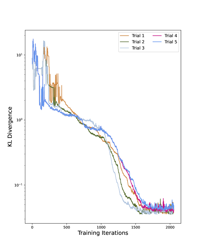
(a) Cardinality Constrained

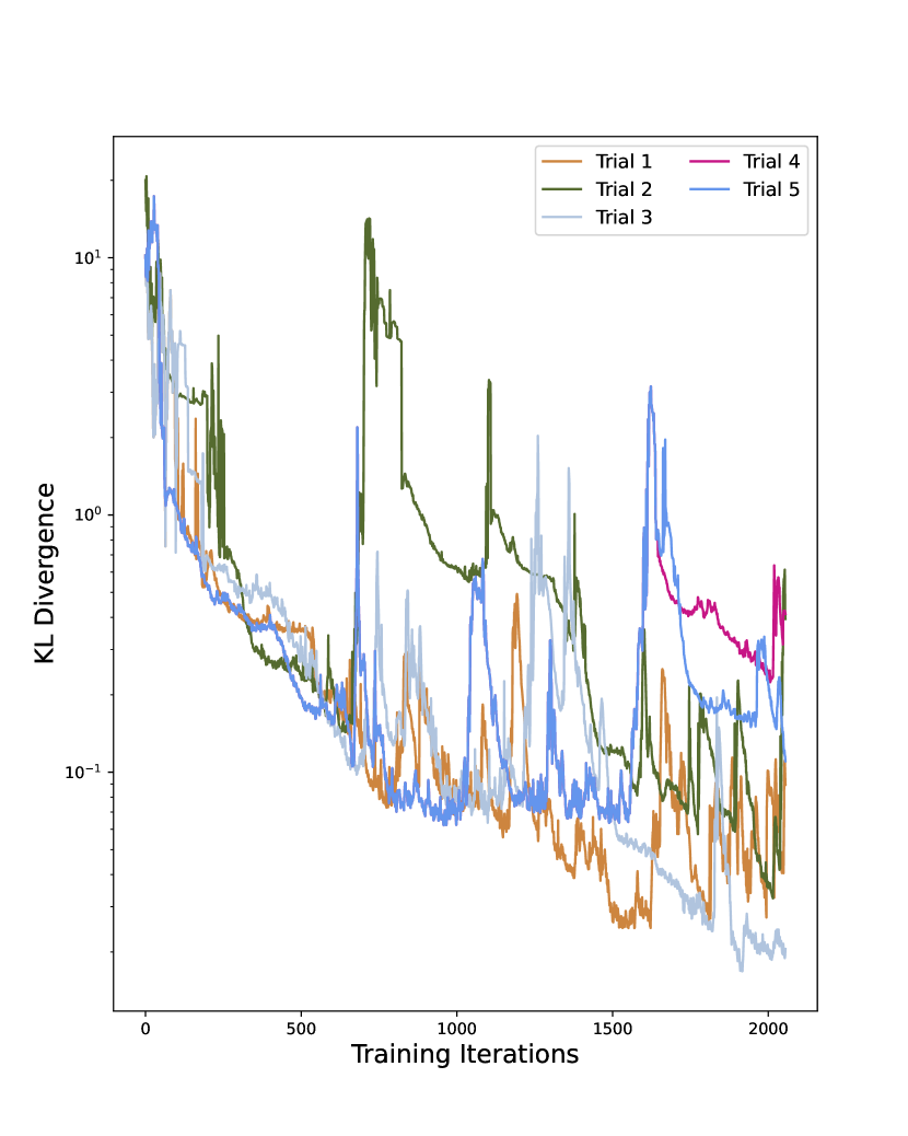
(b) Discrete Gaussian

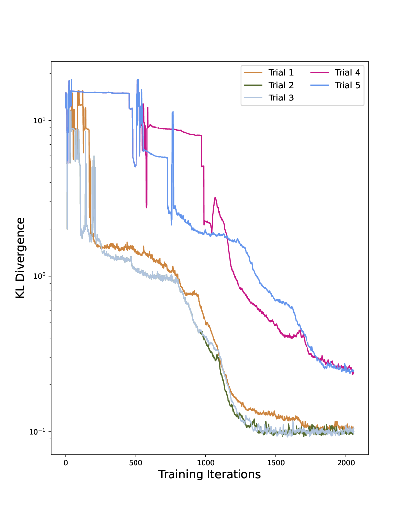
(c) Bars and Stripes

Figure 6: The KL Divergence vs. the number of training iterations for the QNBM across independent trials for three distributions. Here, we see that the QNBM is very stable on all trials of the cardinality-constrained distribution, while it becomes very unstable when learning the discrete Gaussian distribution.

Additionally, we provide evidence that resource allocation when comparing classical and quantum models is of high importance for generating meaningful results. If we had simply allocated resources to the QNBM and the RBM in the same way, the RBM would have performed significantly worse on 2 out of 3 distributions when assessing for learning capability. In Figure 7, we demonstrate the difference between the RBM-2k and the RBM-20k by displaying their output model distributions post-training. Each output distribution displayed is the optimal model chosen from 5 independent trials.

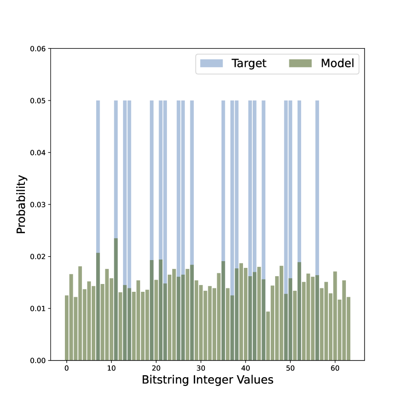
(a) Cardinality: RBM-2k

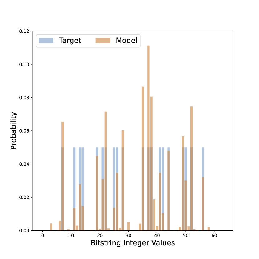
(b) Cardinality: RBM-20k

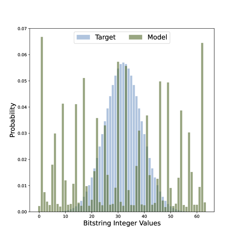
(c) Discrete Gaussian: RBM-2k

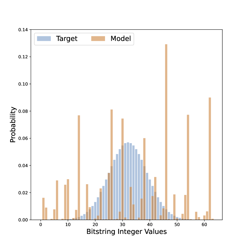
(d) Discrete Gaussian: RBM-20k

(e) Bars and Stripes: RBM-2k

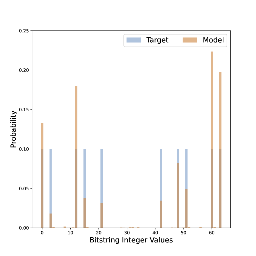
(f) Bars and Stripes: RBM-20k

Figure 7: The best RBM-2k and RBM-20k learning capability on three individual probability distributions. (a) The RBM-2k output distribution overlapped with the cardinality-constrained distribution. (b) The RBM-20k output distribution overlapped with the cardinality-constrained distribution. (c) The The RBM-2k output distribution overlapped with the discrete Gaussian distribution. (d) The The RBM-20k output distribution overlapped with discrete Gaussian distribution. (e) The RBM-2k output distribution overlapped with the bars and stripes (BS) distribution. (f) The RBM-20k output distribution overlapped with the BAS distribution. Each histogram over the support of discrete bitstrings, represented in integer form, presents the model’s output (RBM-2k: green, RBM-20k: gold) over the target distribution (light blue) to demonstrate the model’s ability to express each distribution post training. The best seeds over 5 independent trainings are shown for all models. We see that the RBM-20k outperforms the RBM-2k on both the cardinality-constrained distribution and BS, whereas the RBM-2k outperforms the RBM-20k on the discrete Gaussian distribution.

The best RBM-2k models are able to achieve values of $KL=1.12$ on the cardinality-constrained distribution, $KL=1.46$ on the discrete Gaussian distribution, and $KL=1.51$ on the BAS distribution. In comparison, the best RBM-20k models are able to achieve values of $KL=0.25$, $KL=4.79$, and $KL=0.34$ on each distribution respectively. Thus, shifting the allocated resources causes a $5.84x$ enhancement on the cardinality distribution and a $4.44x$ enhancement on the BAS distribution. Thus, in keeping the number of resources constant, it is important to consider the selected architecture when deciding the best way to allocate them. Lastly, we provide the generalization performance values across all 5 independent trainings for the distributions $d_{200}$ and $d_{300}$.

Seed	$KL_{train}$	$KL_{true}$
11	0.131	0.211
19	0.231	0.294
20	0.440	0.586
70	0.109	1.722
123	0.186	0.974

Table 1: The final values of $KL_{train}$ and $KL_{true}$ for each independent training after the QNBM trains on each training distribution. The final values of $KL_{train}$ and $KL_{true}$ after training on $d_{200}$. Note that the lowest value of $KL_{true}$ ever attained is 0.211, and in this case we still do not have evidence for generalization as $KL_{true}>KL_{train}$.

Seed	$KL_{train}$	$KL_{true}$
11	0.239	0.454
19	0.105	0.085
20	0.560	0.553
70	0.359	0.353
123	0.206	0.176

Table 2: The final values of $KL_{train}$ and $KL_{true}$ after training on $d_{300}$. Note that in four out of the five independent trainings, the model achieves $KL_{true}<KL_{train}$, providing strong evidence that the QNBM is able to generalise the true distribution when training on $d_{300}$.